the t-test, the paired t-test, and introduction to non-parametric tests july 8, 2004
TRANSCRIPT
The t-test, the paired t-test, The t-test, the paired t-test, and introduction to non-parametric testsand introduction to non-parametric tests
July 8, 2004July 8, 2004

1.1. The t-test:The t-test:for comparing means (averages)for comparing means (averages)

Comparing two meansComparing two means
Is the difference in means that we observe between two groups more than we’d expect to see based on chance alone?
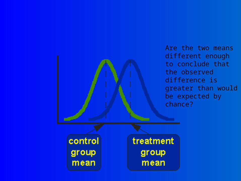
Are the two means different enough to conclude that the observed difference is greater than would be expected by chance?
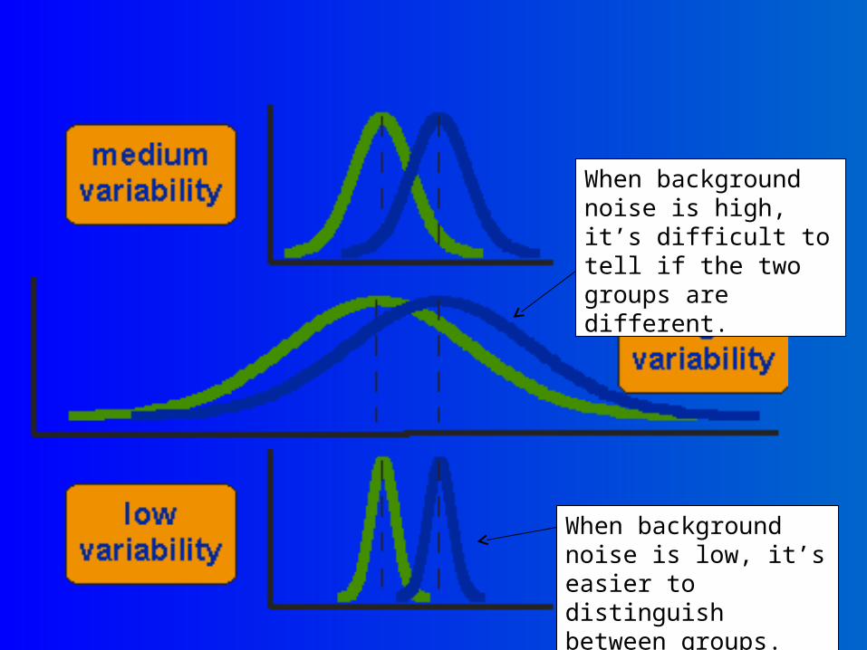
When background noise is high, it’s difficult to tell if the two groups are different.
When background noise is low, it’s easier to distinguish between groups.

Comparing two meansComparing two means
What is the sampling distribution of the difference in the means of two samples?
First we need to know: What is the distribution of a difference between two normally distributed random variables?
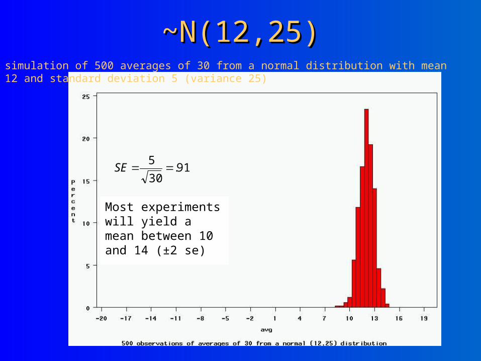
~N(12,25)~N(12,25)simulation of 500 averages of 30 from a normal distribution with mean 12 and standard deviation 5 (variance 25)
91.30
5SE
Most experiments will yield a mean between 10 and 14 (±2 se)

~N(8,25)~N(8,25)simulation of 500 averages of 30 from a normal distribution with mean 8 and standard deviation 5 (variance 25)
91.30
5SE
Most experiments will yield a mean between 6 and 10 (±2 se)
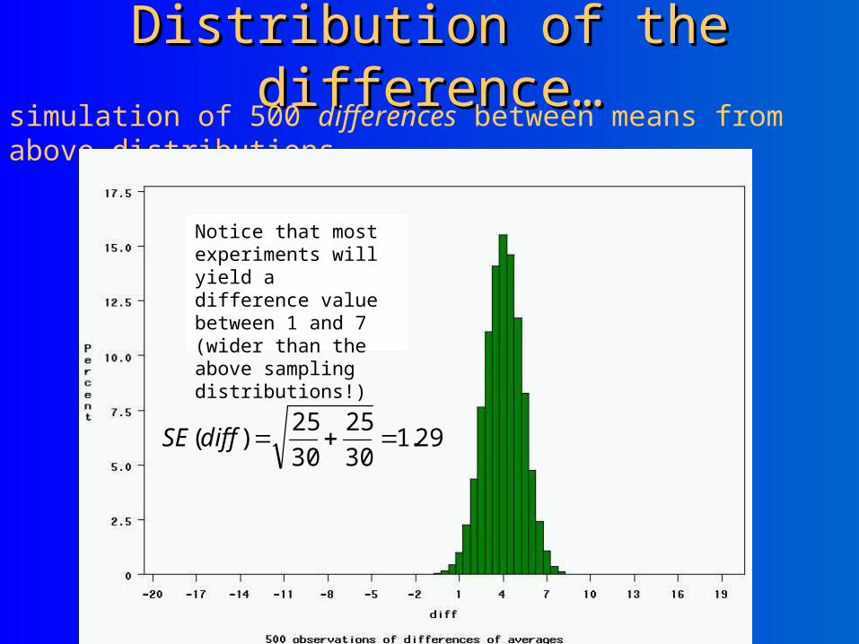
Distribution of the difference…Distribution of the difference…simulation of 500 differences between means from above distributions
29.130
25
30
25)( diffSE
Notice that most experiments will yield a difference value between 1 and 7 (wider than the above sampling distributions!)
Distribution of differencesDistribution of differences
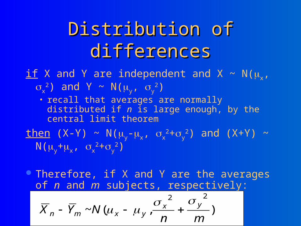
if X and Y are independent and X ~ N(x, x
2) and Y ~ N(y, y2)
• recall that averages are normally distributed if n is large enough, by the central limit theorem
then (X-Y) ~ N(y-x, x2+y
2) and (X+Y) ~ N(y+x, x
2+y2)
Therefore, if X and Y are the averages of n and m subjects, respectively:
),(~22
mnNYX
yxyxmn
ExampleExample
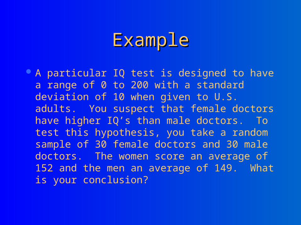
A particular IQ test is designed to have a range of 0 to 200 with a standard deviation of 10 when given to U.S. adults. You suspect that female doctors have higher IQ’s than male doctors. To test this hypothesis, you take a random sample of 30 female doctors and 30 male doctors. The women score an average of 152 and the men an average of 149. What is your conclusion?

Recall steps of a hypothesis Recall steps of a hypothesis test:test:
1. Define your hypotheses (null, alternative)
2. Specify your null distribution:3. Do an experiment4. Calculate the p-value of what
you observed5. Reject or fail to reject (~accept)
the null hypothesis

1.1. Define your Define your hypotheses (null, hypotheses (null,
alternative)alternative)
H0: ♀-doctor IQ = ♂-doctor IQ; (♀ - ♂ = 0)
Ha: ♀-doctor IQ ≠ ♂-doctor IQ; (♀- ♂ ≠ 0 ) [two-sided]
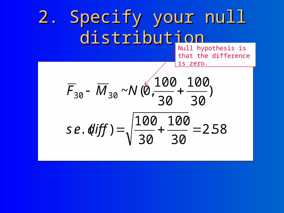
2. Specify your null 2. Specify your null distributiondistribution
58.230
100
30
100).(.
)30
100
30
100,0(~3030
diffes
NMF
Null hypothesis is that the difference is zero.
3. 3. Do an experimentDo an experiment
Observed difference in our experiment = 3.0 IQ points

4.4. Calculate the p-value of Calculate the p-value of what you observed what you observed
3/2.58=1.16
Z = (FROM SAS):
data _null_; x=(1-probnorm(1.16))*2; put x;run;
0.2460488061 (two-sided p-value)
Two sided test! Both tails are possible, so must double the area from one tail.

5.5. Reject or fail to reject Reject or fail to reject (~accept) the null (~accept) the null
hypothesishypothesisNot enough evidence to reject at the .05 significance level. (.24>.05)

Complication 1…Complication 1… The harsh reality is, we hardly ever know the true
standard deviation a priori. If we knew that much, we probably wouldn’t need to run an experiment! In most cases, we must use the sample standard deviation as a stand-in for the truth. However, by estimating the population standard deviation we are adding more uncertainty to our experiment. The null distribution is slightly wider than a normal curve…called a “t-distribution.”

Recall: sample variance and Recall: sample variance and standard deviationstandard deviation
The variance of a population: 2 =
The variance of a sample: s2 =
The standard deviation of a sample: s=
N
xN
ii
2
1
)(
1
)( 2
1
n
xxN
ii
1
)( 2
1
n
xxN
ii

Example: calculation of Example: calculation of sample standard deviationsample standard deviation
systolic blood pressures: 104, 114, 120, 148, 130, 132, 143, 152, 133, 124
Mean = 1300/10 = 130Sample standard deviation =
15230
230110
2070
2070)130124()130133(
)130152()130143()130132(
0)130120()130114()130104(
22
222
222
10
15Estimated standard error of the mean=
Complication 1…Complication 1…The null distribution is slightly wider than a
normal curve…called a “t-distribution.”
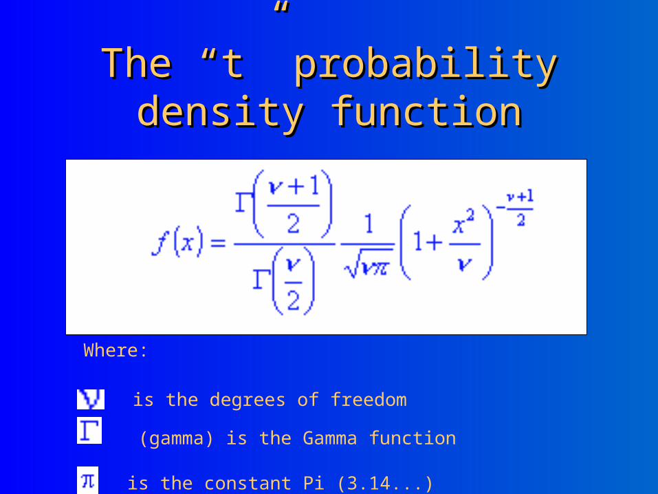
The “t” probability density The “t” probability density functionfunction
Where:
is the degrees of freedom
(gamma) is the Gamma function
is the constant Pi (3.14...)

The “t” distributionsThe “t” distributions The t distribution depends on the degrees of
freedom.
Degrees of freedom here=number of observations used to calculate the standard deviation (n) minus the number of sample means (1 or 2) used in calculation of the sample standard deviation
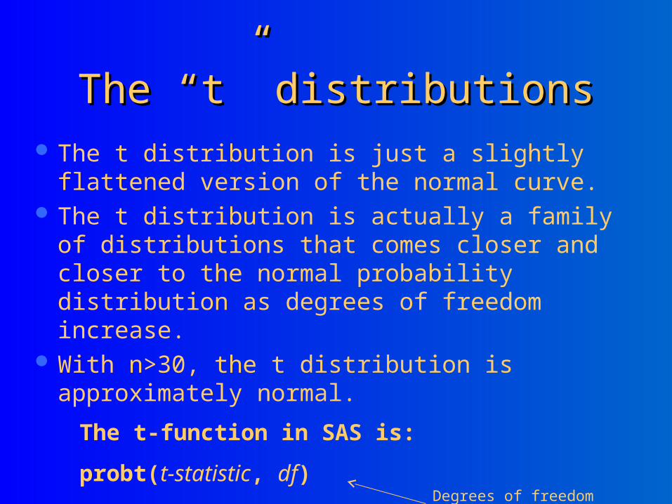
The “t” distributionsThe “t” distributions The t distribution is just a slightly flattened version
of the normal curve. The t distribution is actually a family of distributions
that comes closer and closer to the normal probability distribution as degrees of freedom increase.
With n>30, the t distribution is approximately normal.
The t-function in SAS is:
probt(t-statistic, df) Degrees of freedom
ExampleExample
A one-sample test when the standard deviation is unknown (one-sample t-test)
Example: One sample t-testExample: One sample t-test
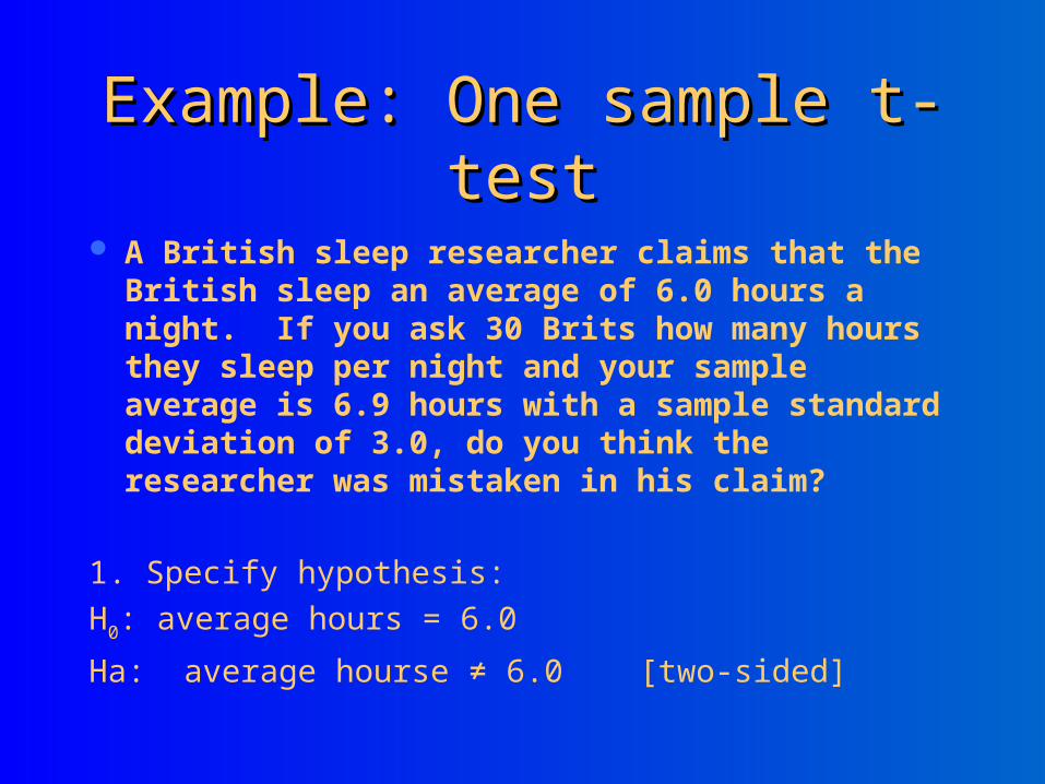
A British sleep researcher claims that the British sleep an average of 6.0 hours a night. If you ask 30 Brits how many hours they sleep per night and your sample average is 6.9 hours with a sample standard deviation of 3.0, do you think the researcher was mistaken in his claim?
1. Specify hypothesis:
H0: average hours = 6.0
Ha: average hourse ≠ 6.0 [two-sided]

One sample t-testOne sample t-test
2. Specify null distribution.The null distribution here actually follows a “t-distribution with 29 (=n-1) “degrees of freedom” (the higher the number of degrees of freedom, the more the t-distribution looks like a normal curve).
)55.030
0.3,0.6(~ 2930 TX
One sample t-testOne sample t-test
3. Observed data=6.9 hours with a sample standard of 3.0
One sample t-testOne sample t-test
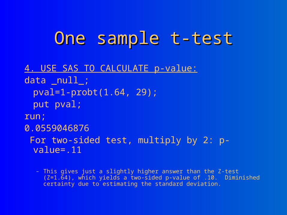
4. USE SAS TO CALCULATE p-value:data _null_;pval=1-probt(1.64, 29);put pval;
run;0.0559046876 For two-sided test, multiply by 2: p-value=.11
– This gives just a slightly higher answer than the Z-test (Z=1.64), which yields a two-sided p-value of .10. Diminished certainty due to estimating the standard deviation.
One sample t-testOne sample t-test
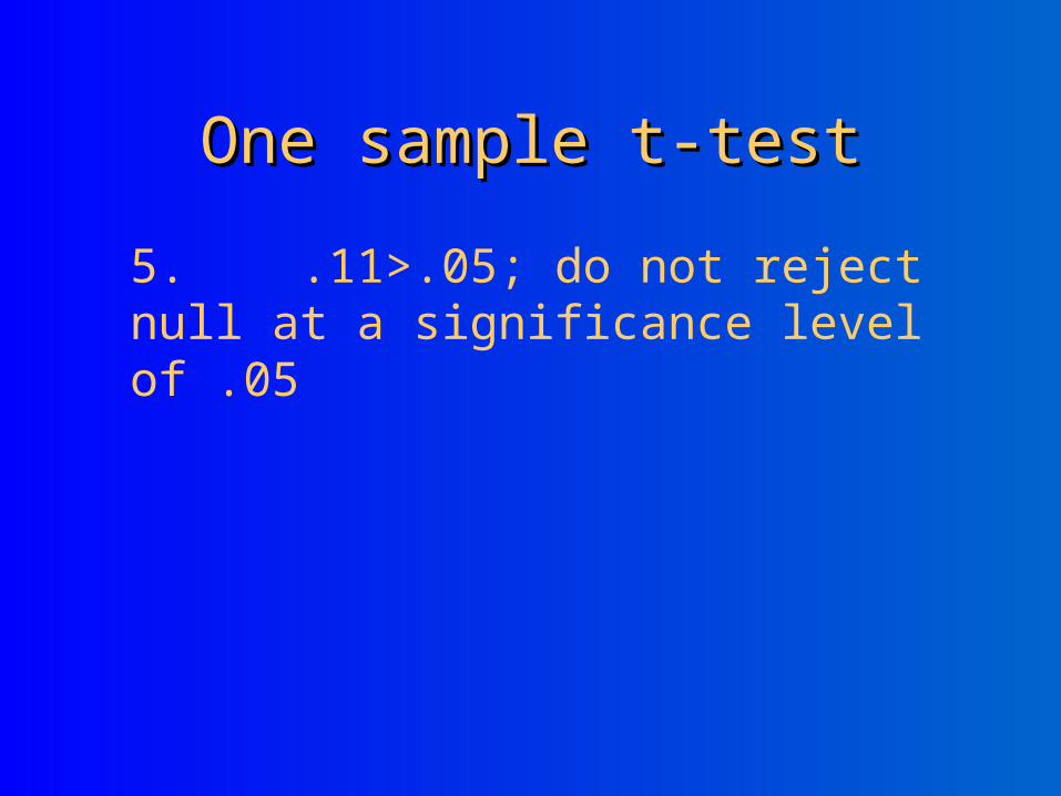
5. .11>.05; do not reject null at a significance level of .05
Example: two-sample t-testExample: two-sample t-test
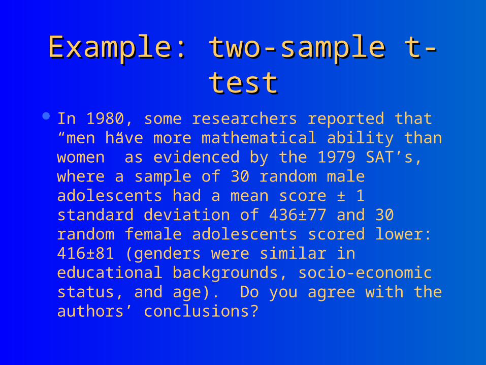
In 1980, some researchers reported that “men have more mathematical ability than women” as evidenced by the 1979 SAT’s, where a sample of 30 random male adolescents had a mean score ± 1 standard deviation of 436±77 and 30 random female adolescents scored lower: 416±81 (genders were similar in educational backgrounds, socio-economic status, and age). Do you agree with the authors’ conclusions?

Two-sample t-testTwo-sample t-test
1. Define your hypotheses (null, alternative)
H0: ♂-♀ math SAT = 0
Ha: ♂-♀ math SAT ≠ 0 [two-sided]
Two-sample t-testTwo-sample t-test
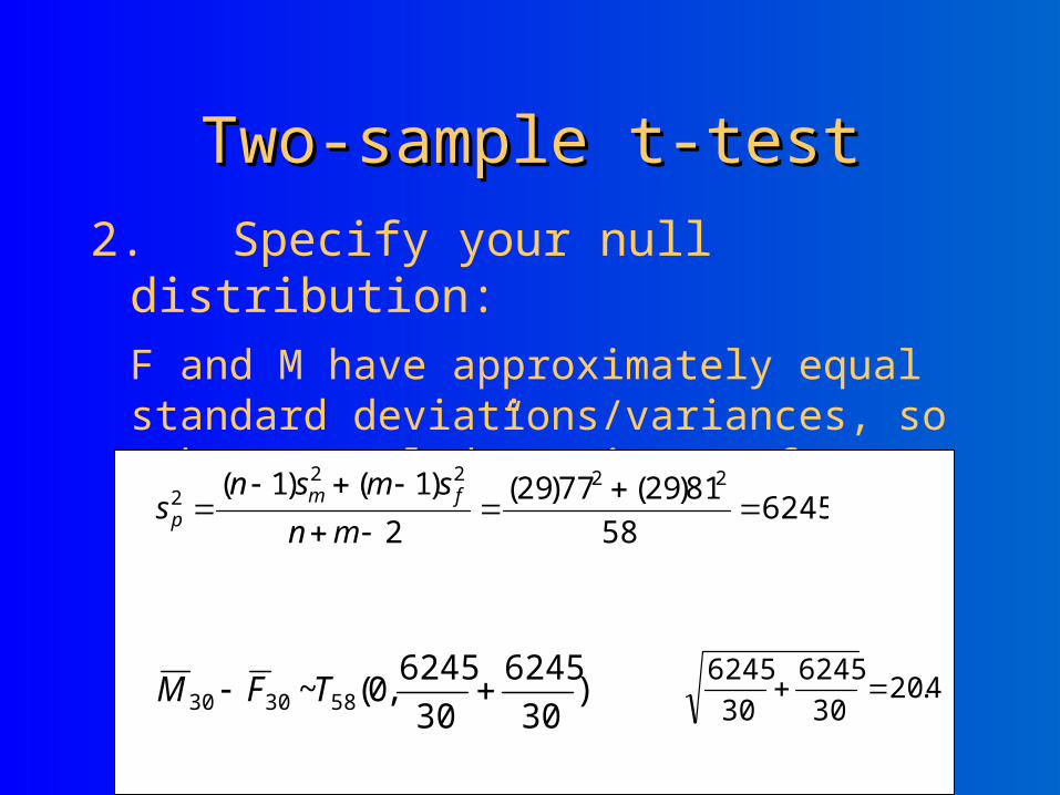
2. Specify your null distribution:
F and M have approximately equal standard deviations/variances, so make a “pooled” estimate of variance.
624558
81)29(77)29(
2
)1()1( 22222
mn
smsns fm
p
)30
6245
30
6245,0(~ 583030 TFM 4.20
30
6245
30
6245

Two-sample t-testTwo-sample t-test
3. Observed difference in our experiment = 20 points
Two-sample t-testTwo-sample t-test
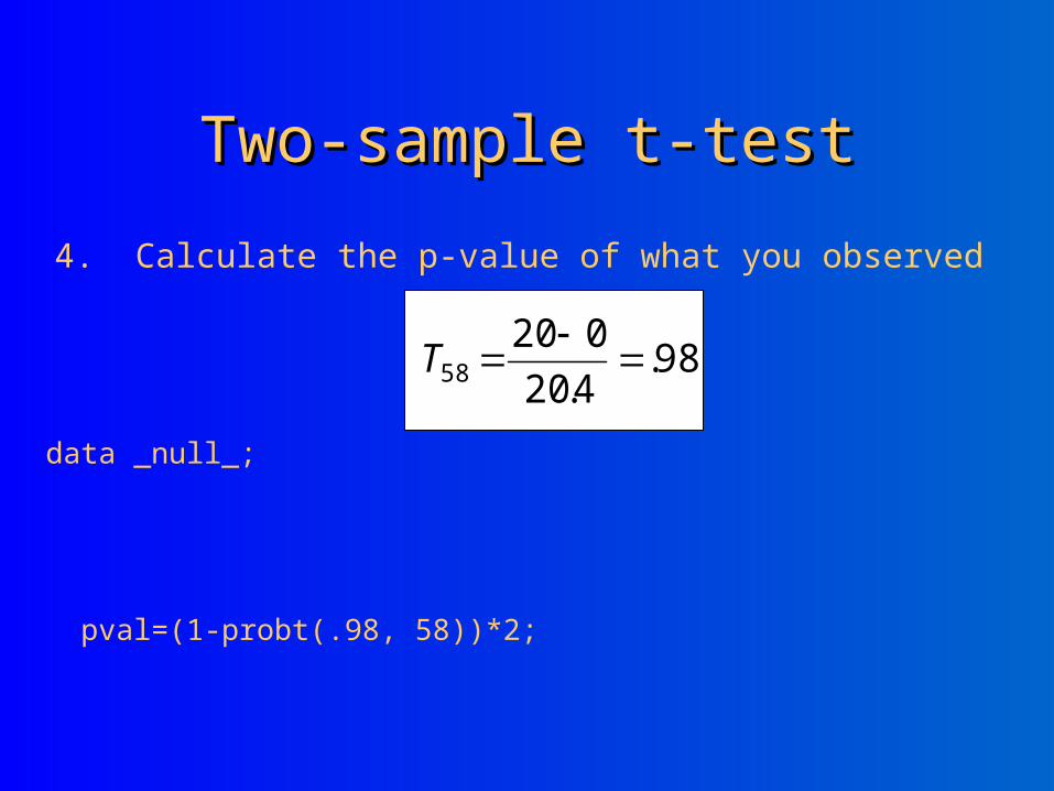
4. Calculate the p-value of what you observed
98.4.20
02058
T
data _null_;
pval=(1-probt(.98, 58))*2;
put pval;
run; 0.3311563454
5. Do not reject null! No evidence that men are better in math ;)
Example 2Example 2
Example: Rosental, R. and Jacobson, L. (1966) Teachers’ expectancies: Determinates of pupils’ I.Q. gains. Psychological Reports, 19, 115-118.

The Experiment The Experiment (note: exact numbers have been altered)(note: exact numbers have been altered)
Grade 3 at Oak School were given an IQ test at the beginning of the academic year (n=90).
Classroom teachers were given a list of names of students in their classes who had supposedly scored in the top 20 percent; these students were identified as “academic bloomers” (n=18).
BUT: the children on the teachers lists had actually been randomly assigned to the list.
At the end of the year, the same I.Q. test was re-administered.

The resultsThe results
Children who had been randomly assigned to the “top-20 percent” list had mean I.Q. increase of 12.2 points (sd=2.0) vs. children in the control group only had an increase of 8.2 points (sd=2.5)
Is this a statistically significant difference? Give a confidence interval for this difference.

1. Hypotheses1. Hypotheses
H0: mean change (“gifted”) – mean change
(control) = 0
Ha: mean change (“gifted”) – mean change (control) ≠ 0

2. Null distribution2. Null distribution
Null distribution of difference of two means:
81.588
5.2)71(0.2)17( 222
ps
)72
81.5
18
81.5,0(~ 88"" Tcontrolgifted
64.72
81.5
18
81.5
3. Empirical data3. Empirical data
Observed difference in our experiment = 12.2-8.2 = 4.0
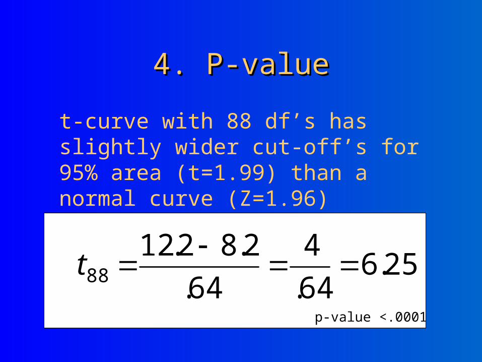
4. P-value4. P-value
t-curve with 88 df’s has slightly wider cut-off’s for 95% area (t=1.99) than a normal curve (Z=1.96)
p-value <.0001
25.664.
4
64.
2.82.1288
t
5. Reject null!5. Reject null!
Conclusion: I.Q. scores can bias expectancies in the teachers’ minds and cause them to unintentionally treat “bright” students differently from those seen as less bright.
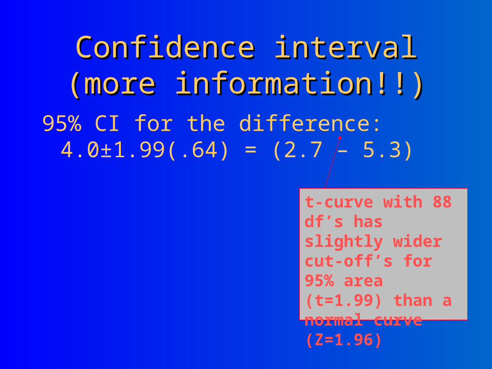
Confidence interval (more Confidence interval (more information!!)information!!)
95% CI for the difference: 4.0±1.99(.64) = (2.7 – 5.3)
t-curve with 88 df’s has slightly wider cut-off’s for 95% area (t=1.99) than a normal curve (Z=1.96)

2. The paired T-test2. The paired T-test

The Paired T-testThe Paired T-test
Paired data: either the same person on different occasions or pairs of people who are more similar to each other than to individuals from other pairs (husband-wife pairs, twin pairs, matched cases and controls, etc.)
For example, evaluates whether an observed change in mean (before vs. after) represents a true improvement (or decrease).
Null hypothesis: difference (after-before)=0

Did the control group in the Did the control group in the previous experiment improveprevious experiment improve
at allat all during the year? during the year?
2829.
2.8
725.2
2.8271 t
p-value <.0001
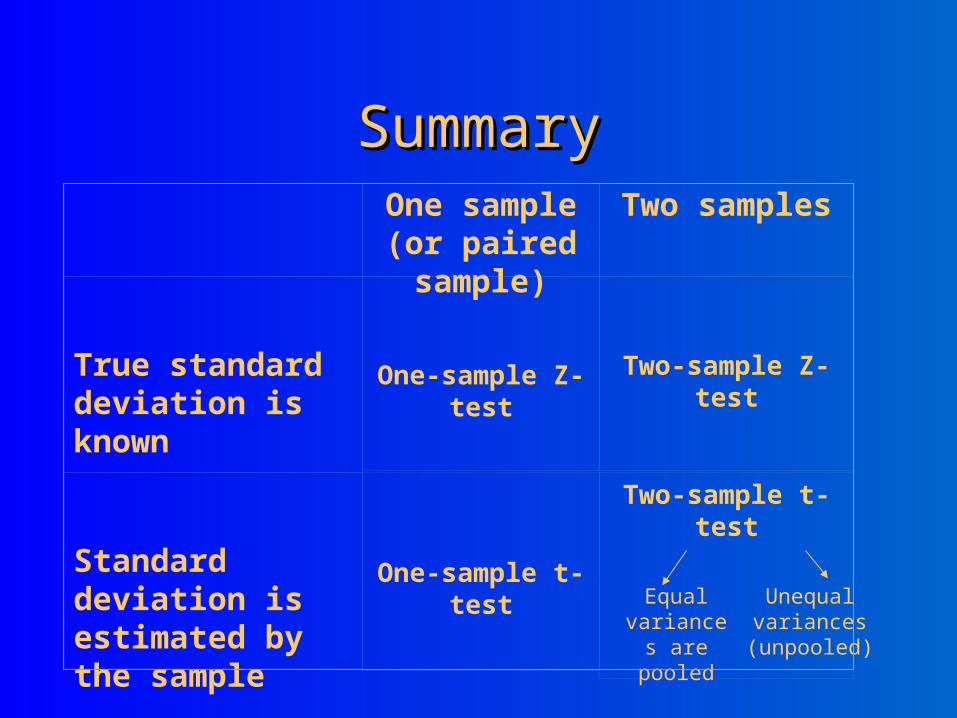
SummarySummary
Equal variances
are pooled
Unequal variances (unpooled)
One sample (or paired sample)
Two samples
True standard deviation is known
One-sample Z-test
Two-sample Z-test
Standard deviation is estimated by the sample
One-sample t-test
Two-sample t-test
Non-parametric testsNon-parametric tests
t-tests require your outcome variable to be normally distributed (or close enough).
Non-parametric tests are based on RANKS instead of means and standard deviations (=“population parameters”).
Example: non-parametric testsExample: non-parametric tests
10 dieters following Atkin’s diet vs. 10 dieters following Jenny Craig
Hypothetical RESULTS:Atkin’s group loses an average of 34.5 lbs.
J. Craig group loses an average of 18.5 lbs.
Conclusion: Atkin’s is better?
Example: non-parametric testsExample: non-parametric tests
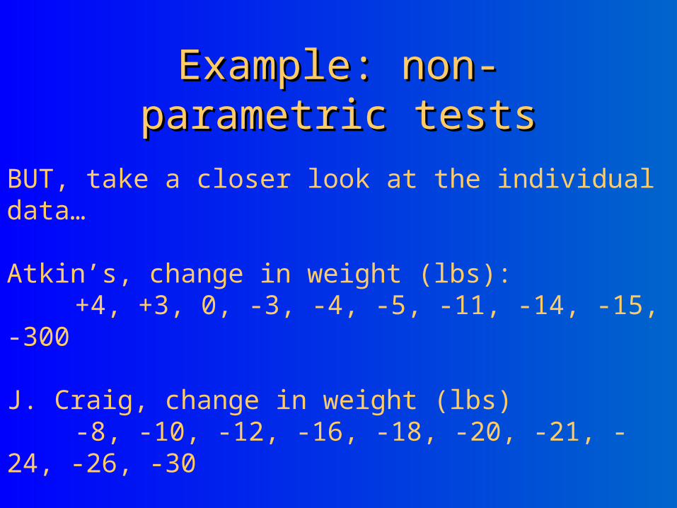
BUT, take a closer look at the individual data…
Atkin’s, change in weight (lbs):+4, +3, 0, -3, -4, -5, -11, -14, -15, -300
J. Craig, change in weight (lbs)-8, -10, -12, -16, -18, -20, -21, -24, -26, -30

Jenny CraigJenny Craig
-30 -25 -20 -15 -10 -5 0 5 10 15 20
0
5
10
15
20
25
30
Percent
Weight Change

Atkin’sAtkin’s
-300 -280 -260 -240 -220 -200 -180 -160 -140 -120 -100 -80 -60 -40 -20 0 20
0
5
10
15
20
25
30
Percent
Weight Change
t-test doesn’t work…t-test doesn’t work…
Comparing the mean weight loss of the two groups is not appropriate here.
The distributions do not appear to be normally distributed.
Moreover, there is an extreme outlier (this outlier influences the mean a great deal).

Statistical tests to compare Statistical tests to compare ranks:ranks:
Wilcoxon Mann-Whitney test is analogue of two-sample t-test.

Wilcoxon Mann-Whitney testWilcoxon Mann-Whitney test
RANK the values, 1 being the least weight loss and 20 being the most weight loss.
Atkin’s +4, +3, 0, -3, -4, -5, -11, -14, -15, -300 1, 2, 3, 4, 5, 6, 9, 11, 12, 20 J. Craig -8, -10, -12, -16, -18, -20, -21, -24, -26, -30 7, 8, 10, 13, 14, 15, 16, 17, 18, 19

Wilcoxon Mann-Whitney testWilcoxon Mann-Whitney test
Sum of Atkin’s ranks: 1+ 2 + 3 + 4 + 5 + 6 + 9 + 11+ 12 + 20=73Sum of Jenny Craig’s ranks:
7 + 8 +10+ 13+ 14+ 15+16+ 17+ 18+19=137
Jenny Craig clearly ranked higher!P-value *(from computer) = .018