the systems biology cycle: computational workflow
TRANSCRIPT

Why Uncertainty Quantification? The Systems Biology Cycle Polynomial Chaos Expansion PCE for correlated inputs
THE SYSTEMS BIOLOGY CYCLE:Computational Workflow & Uncertainty
Quantification
Maria [email protected]
Centrum Wiskunde & InformaticaAmsterdam
Scientific Meeting 06/06/2014
M. Navarro Centrum Wiskunde & InformaticaAmsterdam
The Systems Biology Cycle: UQ

Why Uncertainty Quantification? The Systems Biology Cycle Polynomial Chaos Expansion PCE for correlated inputs
INTRODUCCTION
Postdoc in the Scientific Computing for Systems Biology /Life Science (LS)BioPreDyn: From Data to Models (European project,FP7,#289434) with J.G. Blom and A.T. Valderrama
M. Navarro Centrum Wiskunde & InformaticaAmsterdam
The Systems Biology Cycle: UQ

Why Uncertainty Quantification? The Systems Biology Cycle Polynomial Chaos Expansion PCE for correlated inputs
OUTLINE
1 WHY UNCERTAINTY QUANTIFICATION?
2 THE SYSTEMS BIOLOGY CYCLE
3 POLYNOMIAL CHAOS EXPANSION
4 PCE FOR CORRELATED INPUTS
M. Navarro Centrum Wiskunde & InformaticaAmsterdam
The Systems Biology Cycle: UQ

Why Uncertainty Quantification? The Systems Biology Cycle Polynomial Chaos Expansion PCE for correlated inputs
Errors
M. Navarro Centrum Wiskunde & InformaticaAmsterdam
The Systems Biology Cycle: UQ

Why Uncertainty Quantification? The Systems Biology Cycle Polynomial Chaos Expansion PCE for correlated inputs
Errors
Experimental models: controlled version of realitymodel organisms, synthetic biology
M. Navarro Centrum Wiskunde & InformaticaAmsterdam
The Systems Biology Cycle: UQ

Why Uncertainty Quantification? The Systems Biology Cycle Polynomial Chaos Expansion PCE for correlated inputs
Errors
Mathematical models: precise description of an approximation of realityassumptions, equations
M. Navarro Centrum Wiskunde & InformaticaAmsterdam
The Systems Biology Cycle: UQ

Why Uncertainty Quantification? The Systems Biology Cycle Polynomial Chaos Expansion PCE for correlated inputs
Errors
Computational models: implementation of mathematical modelequation-based, model identification, verification, validation
M. Navarro Centrum Wiskunde & InformaticaAmsterdam
The Systems Biology Cycle: UQ

Why Uncertainty Quantification? The Systems Biology Cycle Polynomial Chaos Expansion PCE for correlated inputs
Errors
(Controllable) errors everywhere
THINK before you do
M. Navarro Centrum Wiskunde & InformaticaAmsterdam
The Systems Biology Cycle: UQ

Why Uncertainty Quantification? The Systems Biology Cycle Polynomial Chaos Expansion PCE for correlated inputs
Errors
(Controllable) errors everywhereTHINK before you do
M. Navarro Centrum Wiskunde & InformaticaAmsterdam
The Systems Biology Cycle: UQ

Why Uncertainty Quantification? The Systems Biology Cycle Polynomial Chaos Expansion PCE for correlated inputs
1 WHY UNCERTAINTY QUANTIFICATION?
2 THE SYSTEMS BIOLOGY CYCLE
3 POLYNOMIAL CHAOS EXPANSION
4 PCE FOR CORRELATED INPUTS
M. Navarro Centrum Wiskunde & InformaticaAmsterdam
The Systems Biology Cycle: UQ

Why Uncertainty Quantification? The Systems Biology Cycle Polynomial Chaos Expansion PCE for correlated inputs
M. Navarro Centrum Wiskunde & InformaticaAmsterdam
The Systems Biology Cycle: UQ

Why Uncertainty Quantification? The Systems Biology Cycle Polynomial Chaos Expansion PCE for correlated inputs
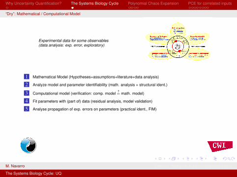
“Dry”: Mathematical / Computational Model
Experimental data for some observables(data analysis: exp. error, exploratory)
1 Mathematical Model (Hypotheses+assumptions+literature+data analysis)
2 Analyze model and parameter identifiability (math. analysis + structural ident.)
3 Computational model (verification: comp. model ?= math. model)
4 Fit parameters with (part of) data (residual analysis, model validation)
5 Analyse propagation of exp. errors on parameters (practical ident., FIM)
6 (Model discrimination (distinguish between various hypotheses/assumptions))
7 Optimal Experimental Design (experimental options, aim)
8 Model predictions
'
&
$
%Uncertainty Quantification
M. Navarro Centrum Wiskunde & InformaticaAmsterdam
The Systems Biology Cycle: UQ

Why Uncertainty Quantification? The Systems Biology Cycle Polynomial Chaos Expansion PCE for correlated inputs
“Dry”: Mathematical / Computational Model
Experimental data for some observables(data analysis: exp. error, exploratory)
1 Mathematical Model (Hypotheses+assumptions+literature+data analysis)
2 Analyze model and parameter identifiability (math. analysis + structural ident.)
3 Computational model (verification: comp. model ?= math. model)
4 Fit parameters with (part of) data (residual analysis, model validation)
5 Analyse propagation of exp. errors on parameters (practical ident., FIM)
6 (Model discrimination (distinguish between various hypotheses/assumptions))
7 Optimal Experimental Design (experimental options, aim)
8 Model predictions
'
&
$
%Uncertainty Quantification
M. Navarro Centrum Wiskunde & InformaticaAmsterdam
The Systems Biology Cycle: UQ

Why Uncertainty Quantification? The Systems Biology Cycle Polynomial Chaos Expansion PCE for correlated inputs
1 WHY UNCERTAINTY QUANTIFICATION?
2 THE SYSTEMS BIOLOGY CYCLE
3 POLYNOMIAL CHAOS EXPANSION
4 PCE FOR CORRELATED INPUTS
M. Navarro Centrum Wiskunde & InformaticaAmsterdam
The Systems Biology Cycle: UQ

Why Uncertainty Quantification? The Systems Biology Cycle Polynomial Chaos Expansion PCE for correlated inputs
Introduction
Deterministic mathematical model
y′(t) = f(t ,y(t)), y(0) = y0
Uncertainty in initial values or parameters (e.g. from error in data)
ξ (multi-variate) random variable, y(t , ξ) random process:
Stochastic mathematical model
y′(t , ξ) = f(t ,y(t , ξ), ξ), y(0, ξ) = y0(ξ)
How to compute y(t , ξ)?
Polynomial Chaos Expansion
M. Navarro Centrum Wiskunde & InformaticaAmsterdam
The Systems Biology Cycle: UQ

Why Uncertainty Quantification? The Systems Biology Cycle Polynomial Chaos Expansion PCE for correlated inputs
Introduction
Deterministic mathematical model
y′(t) = f(t ,y(t)), y(0) = y0
Uncertainty in initial values or parameters (e.g. from error in data)
ξ (multi-variate) random variable, y(t , ξ) random process:
Stochastic mathematical model
y′(t , ξ) = f(t ,y(t , ξ), ξ), y(0, ξ) = y0(ξ)
How to compute y(t , ξ)? Polynomial Chaos Expansion
M. Navarro Centrum Wiskunde & InformaticaAmsterdam
The Systems Biology Cycle: UQ

Why Uncertainty Quantification? The Systems Biology Cycle Polynomial Chaos Expansion PCE for correlated inputs
Basics
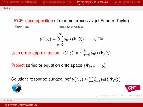
PCE: decomposition of random process y (cf Fourier, Taylor)Wiener (1938) separation of variables
y(t , ξ) =∞∑
p=0
yp(t)Ψp(ξ), ξ RV
Ψ polynomials; orthogonal wrt pdf ρ(ξ)
< Ψi ,Ψj >=
∫S
Ψi(ξ)Ψj(ξ)ρ(ξ)dξ = 0, i 6= j
p̂-th order approximation: y(t , ξ) ≈∑p̂
p=0 yp(t)Ψp(ξ)
Project series or equation onto space {Ψ0, ...,Ψp̂}
Solution: response surface, pdf y(t , ξ) ≈∑p̂
p=0 yp(t)Ψp(ξ)
M. Navarro Centrum Wiskunde & InformaticaAmsterdam
The Systems Biology Cycle: UQ

Why Uncertainty Quantification? The Systems Biology Cycle Polynomial Chaos Expansion PCE for correlated inputs
Basics
PCE: decomposition of random process y (cf Fourier, Taylor)Wiener (1938) separation of variables
y(t , ξ) =∞∑
p=0
yp(t)Ψp(ξ), ξ RV
p̂-th order approximation: y(t , ξ) ≈∑p̂
p=0 yp(t)Ψp(ξ)
Project series or equation onto space {Ψ0, ...,Ψp̂}
Solution: response surface, pdf y(t , ξ) ≈∑p̂
p=0 yp(t)Ψp(ξ)
M. Navarro Centrum Wiskunde & InformaticaAmsterdam
The Systems Biology Cycle: UQ

Why Uncertainty Quantification? The Systems Biology Cycle Polynomial Chaos Expansion PCE for correlated inputs
Basics
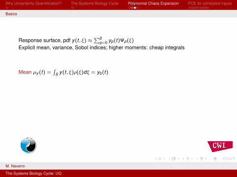
Response surface, pdf y(t , ξ) ≈∑p̂
p=0 yp(t)Ψp(ξ)
Explicit mean, variance, Sobol indices; higher moments: cheap integrals
Mean µy (t) =∫
S y(t , ξ)ρ(ξ)dξ = y0(t)
Variance σ2y (t) =
∫S(y(t , ξ))2ρ(ξ)dξ − µ2
y (t) =∑
p=1 yp(t)2||Ψp||2
Sobol indices Sl (t) = yl (t)2||Ψl ||2
σ2y (t)
first order, independent random variables
M. Navarro Centrum Wiskunde & InformaticaAmsterdam
The Systems Biology Cycle: UQ
Why Uncertainty Quantification? The Systems Biology Cycle Polynomial Chaos Expansion PCE for correlated inputs
Basics
Response surface, pdf y(t , ξ) ≈∑p̂
p=0 yp(t)Ψp(ξ)
Explicit mean, variance, Sobol indices; higher moments: cheap integrals
Mean µy (t) =∫
S y(t , ξ)ρ(ξ)dξ = y0(t)
Variance σ2y (t) =
∫S(y(t , ξ))2ρ(ξ)dξ − µ2
y (t) =∑
p=1 yp(t)2||Ψp||2
Sobol indices Sl (t) = yl (t)2||Ψl ||2
σ2y (t)
first order, independent random variables
M. Navarro Centrum Wiskunde & InformaticaAmsterdam
The Systems Biology Cycle: UQ

Why Uncertainty Quantification? The Systems Biology Cycle Polynomial Chaos Expansion PCE for correlated inputs
Generalizations
n > 1 RVs: multidimensional pdf’s# expansion terms: N = (n+p̂)!
n! p̂!− 1
arbitrarily distributed independent RVsgeneralized Polynomial Chaosarbitrarily multivariate distribution (2014)incl. correlations between RVsIn collaboration with J. Witteveen - Scientific Computing
M. Navarro Centrum Wiskunde & InformaticaAmsterdam
The Systems Biology Cycle: UQ

Why Uncertainty Quantification? The Systems Biology Cycle Polynomial Chaos Expansion PCE for correlated inputs
Generalizations
n > 1 RVs: multidimensional pdf’s# expansion terms: N = (n+p̂)!
n! p̂!− 1
arbitrarily distributed independent RVsgeneralized Polynomial Chaos
arbitrarily multivariate distribution (2014)incl. correlations between RVsIn collaboration with J. Witteveen - Scientific Computing
M. Navarro Centrum Wiskunde & InformaticaAmsterdam
The Systems Biology Cycle: UQ

Why Uncertainty Quantification? The Systems Biology Cycle Polynomial Chaos Expansion PCE for correlated inputs
Generalizations
n > 1 RVs: multidimensional pdf’s# expansion terms: N = (n+p̂)!
n! p̂!− 1
arbitrarily distributed independent RVsgeneralized Polynomial Chaosarbitrarily multivariate distribution (2014)incl. correlations between RVsIn collaboration with J. Witteveen - Scientific Computing
M. Navarro Centrum Wiskunde & InformaticaAmsterdam
The Systems Biology Cycle: UQ

Why Uncertainty Quantification? The Systems Biology Cycle Polynomial Chaos Expansion PCE for correlated inputs
1 WHY UNCERTAINTY QUANTIFICATION?
2 THE SYSTEMS BIOLOGY CYCLE
3 POLYNOMIAL CHAOS EXPANSION
4 PCE FOR CORRELATED INPUTS
M. Navarro Centrum Wiskunde & InformaticaAmsterdam
The Systems Biology Cycle: UQ

Why Uncertainty Quantification? The Systems Biology Cycle Polynomial Chaos Expansion PCE for correlated inputs
Introduction
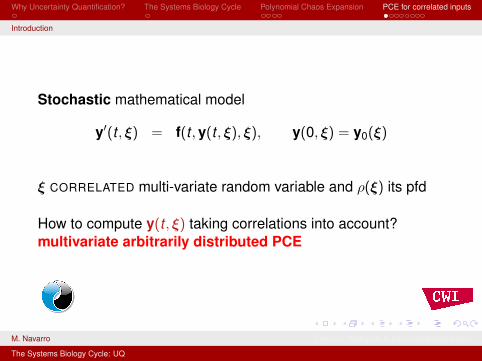
Stochastic mathematical model
y′(t , ξ) = f(t ,y(t , ξ), ξ), y(0, ξ) = y0(ξ)
ξ CORRELATED multi-variate random variable and ρ(ξ) its pfd
How to compute y(t , ξ) taking correlations into account?
multivariate arbitrarily distributed PCE
M. Navarro Centrum Wiskunde & InformaticaAmsterdam
The Systems Biology Cycle: UQ
Why Uncertainty Quantification? The Systems Biology Cycle Polynomial Chaos Expansion PCE for correlated inputs
Introduction
Stochastic mathematical model
y′(t , ξ) = f(t ,y(t , ξ), ξ), y(0, ξ) = y0(ξ)
ξ CORRELATED multi-variate random variable and ρ(ξ) its pfd
How to compute y(t , ξ) taking correlations into account?multivariate arbitrarily distributed PCE
M. Navarro Centrum Wiskunde & InformaticaAmsterdam
The Systems Biology Cycle: UQ
Why Uncertainty Quantification? The Systems Biology Cycle Polynomial Chaos Expansion PCE for correlated inputs
Orthogonal polynomials for correlated inputs
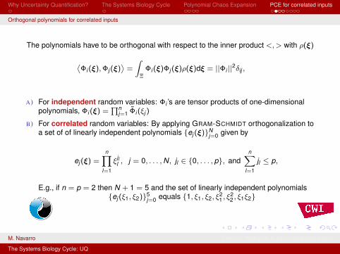
The polynomials have to be orthogonal with respect to the inner product <,> with ρ(ξ)
⟨Φi (ξ),Φj (ξ)
⟩=
∫Ξ
Φi (ξ)Φj (ξ)ρ(ξ)dξ = ||Φi ||2δij ,
A) For independent random variables: Φi ’s are tensor products of one-dimensionalpolynomials, Φi (ξ) =
∏nj=1 Φ̃i (ξj )
B) For correlated random variables: By applying GRAM-SCHMIDT orthogonalization toa set of of linearly independent polynomials {ej (ξ)}N
j=0 given by
ej (ξ) =n∏
l=1
ξjll , j = 0, . . . ,N, jl ∈ {0, . . . , p}, and
n∑l=1
jl ≤ p,
E.g., if n = p = 2 then N + 1 = 5 and the set of linearly independent polynomials{ej (ξ1, ξ2)}5
j=0 equals {1, ξ1, ξ2, ξ21 , ξ
22 , ξ1ξ2}
M. Navarro Centrum Wiskunde & InformaticaAmsterdam
The Systems Biology Cycle: UQ

Why Uncertainty Quantification? The Systems Biology Cycle Polynomial Chaos Expansion PCE for correlated inputs
Orthogonal polynomials for correlated inputs
ORDER 0: % = −0.5 % = 0 % = 0.5
0
1
2
0
1
20
1
2
Ψ0
αβ 0
1
2
0
1
20
1
2
Ψ0
αβ 0
1
2
0
1
20
1
2
Ψ0
αβ
ORDER 1: % = −0.5 % = 0 % = 0.5
0
1
2
0
1
2−2
0
2
αβ
Ψ2
0
1
2
0
1
2−2
0
2
αβ
Ψ2
0
1
2
0
1
2−2
0
2
αβ
Ψ2
ORDER 2: % = −0.5 % = 0 % = 0.5
0
1
2
0
1
2
−1
1
3
αβ
Ψ4
0
1
2
0
1
2
−1
1
3
αβ
Ψ4
0
1
2
0
1
2
−1
1
3
αβ
Ψ4
M. Navarro Centrum Wiskunde & InformaticaAmsterdam
The Systems Biology Cycle: UQ

Why Uncertainty Quantification? The Systems Biology Cycle Polynomial Chaos Expansion PCE for correlated inputs
Orthogonal polynomials for correlated inputs
Explicit mean, variance, Sobol indices
Mean µy (t) =∫
S y(t , ξ)ρ(ξ)dξ = y0(t)
Variance σ2y (t) =
∫S(y(t , ξ))2ρ(ξ)dξ − µ2
y (t) =∑
p=1 yp(t)2||Ψp||2
Sobol indices Sl (t) = Cov[Ml (t,ξl ),y ]
σ2y (t)
= Sul (t) + Sc
l (t), with
Sul (t) =
Var[Eξ¬l[y|ξl ]]
σ2y (t)
, and
Scl (t) =
Cov[Eξ¬l[y|ξl ],y−Eξ¬l
[y|ξl ]]
σ2y (t)
M. Navarro Centrum Wiskunde & InformaticaAmsterdam
The Systems Biology Cycle: UQ

Why Uncertainty Quantification? The Systems Biology Cycle Polynomial Chaos Expansion PCE for correlated inputs
Example
E + Sk1�k2
C,
Ck3→ E + P
Parameter estimationUncertainty in parameters Correlations effect?
M. Navarro Centrum Wiskunde & InformaticaAmsterdam
The Systems Biology Cycle: UQ

Why Uncertainty Quantification? The Systems Biology Cycle Polynomial Chaos Expansion PCE for correlated inputs
Example
E + Sk1�k2
C,
Ck3→ E + P
Parameter estimation
0 5 10 15 20
0
0.1
0.2
0.3
0.4
0.5
0.6
0.7
0.8
0.9
1
Uncertainty in parameters Correlations effect?
M. Navarro Centrum Wiskunde & InformaticaAmsterdam
The Systems Biology Cycle: UQ

Why Uncertainty Quantification? The Systems Biology Cycle Polynomial Chaos Expansion PCE for correlated inputs
Example
E + Sk1�k2
C,
Ck3→ E + P
Parameter estimation
0 5 10 15 20
0
0.1
0.2
0.3
0.4
0.5
0.6
0.7
0.8
0.9
1
Uncertainty in parameters
Correlations effect?
M. Navarro Centrum Wiskunde & InformaticaAmsterdam
The Systems Biology Cycle: UQ

Why Uncertainty Quantification? The Systems Biology Cycle Polynomial Chaos Expansion PCE for correlated inputs
Example
E + Sk1�k2
C,
Ck3→ E + P
Parameter estimation
0 5 10 15 20
0
0.1
0.2
0.3
0.4
0.5
0.6
0.7
0.8
0.9
1
Uncertainty in parameters Correlations effect?
∆I (k1) ∆I (k2) ∆I (k3)
0.295 0.169 0.008
R20 =
1 0.9 −0.370.9 1 −0.45−0.37 −0.45 1
M. Navarro Centrum Wiskunde & InformaticaAmsterdam
The Systems Biology Cycle: UQ

Why Uncertainty Quantification? The Systems Biology Cycle Polynomial Chaos Expansion PCE for correlated inputs
Example
FIGURE : Means
(A) Substrate S (B) Complex C
(C) Enzyme E (D) Product P
M. Navarro Centrum Wiskunde & InformaticaAmsterdam
The Systems Biology Cycle: UQ

Why Uncertainty Quantification? The Systems Biology Cycle Polynomial Chaos Expansion PCE for correlated inputs
Example
FIGURE : Significant qualitative effect of correlation on standard deviation
(A) Substrate S (B) Complex C
M. Navarro Centrum Wiskunde & InformaticaAmsterdam
The Systems Biology Cycle: UQ

Why Uncertainty Quantification? The Systems Biology Cycle Polynomial Chaos Expansion PCE for correlated inputs
Example
FIGURE : Significant qualitative effect of correlation on standard deviation
(A) Enzyme E (B) Product P
M. Navarro Centrum Wiskunde & InformaticaAmsterdam
The Systems Biology Cycle: UQ

Why Uncertainty Quantification? The Systems Biology Cycle Polynomial Chaos Expansion PCE for correlated inputs
CONCLUSIONS AND FUTURE WORKS
Study the UQ of the QoIs helps us to know the quality ofthe model predictionsSobol indices: ranking influence of RVs (uncertainparameters)→ reductionTake correlations into accountDevelop Gauss quadrature based on new polynomials
M. Navarro Centrum Wiskunde & InformaticaAmsterdam
The Systems Biology Cycle: UQ

Why Uncertainty Quantification? The Systems Biology Cycle Polynomial Chaos Expansion PCE for correlated inputs
Thank you
M. Navarro Centrum Wiskunde & InformaticaAmsterdam
The Systems Biology Cycle: UQ