the strategic use of private quality standards in food
TRANSCRIPT

The Strategic Use of Private Quality Standards in
Food Supply Chains�
Vanessa von Schlippenbachy Isabel Teichmannz
May 2012
Abstract
We explore the strategic role of private quality standards in food supply chains.Considering two symmetric retailers that are exclusively supplied by a �nitenumber of producers and endogenizing the suppliers�delivery choice, we showthat there exist two asymmetric equilibria in the retailers�quality requirements.Our results reveal that the retailers use private quality standards to improvetheir bargaining position in the intermediate goods market. This is associ-ated with ine¢ ciencies in the upstream production, which can be mitigated byenforcing a minimum quality standard.
JEL Classi�cation: L15, L42, Q13
Keywords: private quality standards, vertical relations, buyer power, food supplychain
�We would like to thank David Hennessy and two anonymous referees for their valuable com-ments. Furthermore, we are grateful to Pio Baake, Özlem Bedre-Defolie, Stéphane Caprice, ClaireChambolle, Clémence Christin and Vincent Réquillart, as well as participants of the Annual Con-ference of the GeWiSoLa (Halle, 2011), of the EAAE Congress (Zurich, 2011), of the Verein fürSocialpolitik (Kiel, 2010), and seminar participants at DIW Berlin, Humboldt-Universität zu Berlin,Toulouse School of Economics and INRA-ALISS Paris for helpful discussions and suggestions. Finan-cial support from the Deutsche Forschungsgemeinschaft (FOR 986 and "Market Power in VerticallyRelated Markets") is gratefully acknowledged.
yCorresponding Author: Deutsches Institut für Wirtschaftsforschung (DIW) Berlin and Univer-sity of Düsseldorf, Düsseldorf Institute for Competition Economics (DICE), e-mail: [email protected]
zDeutsches Institut für Wirtschaftsforschung (DIW) Berlin and Humboldt-Universität zu Berlin,e-mail: [email protected]
1
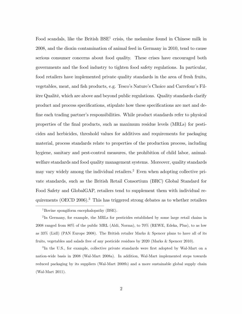
Food scandals, like the British BSE1 crisis, the melamine found in Chinese milk in
2008, and the dioxin contamination of animal feed in Germany in 2010, tend to cause
serious consumer concerns about food quality. These crises have encouraged both
governments and the food industry to tighten food safety regulations. In particular,
food retailers have implemented private quality standards in the area of fresh fruits,
vegetables, meat, and �sh products, e.g. Tesco�s Nature�s Choice and Carrefour�s Fil-
ière Qualité, which are above and beyond public regulations. Quality standards clarify
product and process speci�cations, stipulate how these speci�cations are met and de-
�ne each trading partner�s responsibilities. While product standards refer to physical
properties of the �nal products, such as maximum residue levels (MRLs) for pesti-
cides and herbicides, threshold values for additives and requirements for packaging
material, process standards relate to properties of the production process, including
hygiene, sanitary and pest-control measures, the prohibition of child labor, animal-
welfare standards and food quality management systems. Moreover, quality standards
may vary widely among the individual retailers.2 Even when adopting collective pri-
vate standards, such as the British Retail Consortium (BRC) Global Standard for
Food Safety and GlobalGAP, retailers tend to supplement them with individual re-
quirements (OECD 2006).3 This has triggered strong debates as to whether retailers
1Bovine spongiform encephalopathy (BSE).
2In Germany, for example, the MRLs for pesticides established by some large retail chains in
2008 ranged from 80% of the public MRL (Aldi, Norma), to 70% (REWE, Edeka, Plus), to as low
as 33% (Lidl) (PAN Europe 2008). The British retailer Marks & Spencer plans to have all of its
fruits, vegetables and salads free of any pesticide residues by 2020 (Marks & Spencer 2010).
3In the U.S., for example, collective private standards were �rst adopted by Wal-Mart on a
nation-wide basis in 2008 (Wal-Mart 2008a). In addition, Wal-Mart implemented steps towards
reduced packaging by its suppliers (Wal-Mart 2008b) and a more sustainable global supply chain
(Wal-Mart 2011).
2

use private quality standards as a strategic instrument to gain buyer power in pro-
curement markets.4 So far, this conjecture has not been formally analyzed.5 We
intend to narrow this gap by investigating the retailers�quality choice in a vertical
bargaining setting.
More precisely, we consider a vertical structure with two downstream retailers that
are supplied by a �nite number of upstream producers with increasing marginal costs
of production. The retailers are assumed to impose private quality requirements
that must be ful�lled by their respective suppliers. Taking the retailers� quality
standards as given, the upstream producers decide which retailer they exclusively
supply and, thus, which quality standard they meet. Compliance with a higher quality
standard is associated with higher quality costs.6 Furthermore, the suppliers are not
4Further incentives for retailers to set private quality standards might be to prevent a potential
decrease in revenue due to reputation losses (OECD 2006), to respond to public minimum stan-
dards (e.g., Valletti 2000; Crampes and Hollander 1995; Ronnen 1991), to pre-empt or in�uence
public regulation (e.g., McCluskey and Winfree 2009; Lutz, Lyon and Maxwell 2000), to counter
producers�lobbying for low public minimum quality standards (Vandemoortele 2011), to substitute
for inadequate public regulation in developing countries (e.g., Marcoul and Veyssiere 2010), or to
safeguard against liability claims (e.g., Giraud-Héraud, Hammoudi and Soler 2006; Giraud-Héraud
et al. 2008). There is also a �erce debate on whether increasing quality requirements by large
retailers may impose entry barriers for suppliers in developing countries, in particular for small-scale
producers (e.g., OECD 2007, 2006; García Martinez and Poole 2004; Balsevich et al. 2003; Boselie,
Henson and Weatherspoon 2003).
5Hammoudi, Ho¤mann and Surry (2009) even state that the understanding of the strategic
aspects of private quality standards in vertical relations is still underdeveloped.
6Production costs in the food sector are increasing in quality due to the necessary replacement
of pesticides, herbicides or fertilizer by more expensive raw materials, increased management duties
and higher labor inputs. Further quality-related cost increases are associated with the development
and implementation of quality-management systems, stricter testing and documentation, changes in
the production processes, and certi�cation requirements.
3

able to adjust the quality of their production in the short-term since the product
quality depends on the underlying production processes. Given the retailers�quality
requirements and the suppliers�delivery decision, both retailers enter into bilateral
negotiations with their respective suppliers about the delivery conditions. If a supplier
fails to �nd an agreement with its selected retailer, it is able to switch the delivery
to the other retailer as long as it complies with the respective quality requirements.
Upon successful completion of the negotiations, each supplier produces and delivers
its product to the retailer. Each retailer transforms the received inputs into a �nal
good and sells it to consumers in a perfectly competitive market.
We �nd that there exist two asymmetric equilibria in the retailers�quality choice.
If one retailer sets a relatively high quality standard, the other retailer has an incen-
tive to undercut this quality requirement. The reason is that the suppliers cannot
adjust their product quality in the short-term. Accordingly, the suppliers complying
with the lower quality standard lose their outside option, which improves the bar-
gaining position of the low-quality retailer. In turn, if one retailer sets a relatively
low quality standard, the other retailer has an incentive to implement stricter quality
requirements. By increasing its quality standard, the high-quality retailer weakens
the outside option of its suppliers since they incur the production costs for the high
quality standard but are rewarded for the lower quality only when supplying the low-
quality retailer. This improves the bargaining position of the high-quality retailer. In
equilibrium, more suppliers decide to deliver to the high-quality retailer than to the
low-quality retailer. This induces ine¢ ciencies in the upstream market as an e¢ cient
production structure requires that both retailers set the same quality standard and
the suppliers split equally between the retailers. Overall, our analysis reveals that
the retailers use the private quality standards as a strategic instrument to improve
their bargaining position in the intermediate goods market, resulting in ine¢ cient
4

upstream production.
Although quality standards are receiving growing attention, few articles address
retailers�private standards in vertical relations.7 Insights can be found in studies on
premium private labels (PPLs). Considering a vertical chain with a �nite number of
upstream producers delivering to a �nite number of local retail monopolies via a spot
market, Giraud-Héraud, Rouached and Soler (2006) analyze the incentive of a retailer
to establish a PPL, which is based on direct contracting between the retailer and its
PPL suppliers. They �nd that the incentive for a retailer to di¤erentiate its business
via a PPL is the higher the lower the public minimum quality standard (MQS). In
a similar framework, Bazoche, Giraud-Héraud and Soler (2005) analyze the interest
of producers to commit to a retailer�s PPL. They show that fewer producers have an
incentive to deliver the PPL when the quality of the MQS is increasing. Furthermore,
they �nd that the introduction of a PPL results in higher prices in the intermediate
goods market. In contrast to our �ndings, however, both articles show that the aim
of a PPL is not to increase the bargaining power of the retailer.8
Our analysis is also related to the large theoretical literature on the sources of
buyer power. Potential sources of buyer power include credible threats to vertically
integrate or to support market entry at the upstream level (e.g., Katz 1987; She¤man
7For example, Valletti (2000), Crampes and Hollander (1995) and Ronnen (1991) analyze private
standard setting in response to the introduction of a public minimum standard. Focussing on product
di¤erentiation, private quality decisions of �rms are also studied by Motta (1993) and Gal-Or (1985,
1987). However, all these papers neglect vertical supply structures.
8Collective standard setting of retailers is analyzed by Giraud-Héraud, Hammoudi and Soler
(2006) as well as Giraud-Héraud et al. (2008). Both articles analyze the introduction of a collective
standard for a given public MQS, assuming that retailers are price takers in the procurement market.
In their models, the retailers�incentive to implement a collective standard depends on the existence
of a legal liability rule.
5

and Spiller 1992), potential delisting strategies after downstream mergers (e.g., In-
derst and Sha¤er 2007), producers�di¤erentiation (Chambolle and Berto Villas-Boas
2010) as well as a greater degree of retailers�di¤erentiation compared to producers�
di¤erentiation (Allain 2002).9 We show that downstream �rms�quality requirements
may constitute an additional source of buyer power.
The remainder of the article is organized as follows. First, we present our model.
Subsequently, we conduct the equilibrium analysis and investigate the private quality
standards of the retailers under perfect competition. To check the robustness of our
results, we further extend our analysis to imperfect competition. Finally, we conclude
and derive the relevant policy implications.
The Model
We consider a food supply chain with two symmetric downstream retailersDi, i = 1; 2,
and N � 2 symmetric upstream suppliers. Each retailer implements a private quality
standard qi; which has to be met by their respective suppliers. The higher qi, the more
demanding the quality requirements. Taking as given the retailers�private quality
standards, the N upstream �rms decide which retailer they supply and, thus, which
quality standard they comply with. Let Uij denote the suppliers that deliver to retailer
Di:Without loss of generality, we assume that the N1 upstream �rms U11; :::; U1N1 sell
exclusively to the downstream �rm D1; while the remaining N2 = N �N1 upstream
�rms U2N1+1; :::; U2N deliver exclusively to the downstream �rm D2. The delivery
conditions are based on bilateral and simultaneous negotiations between the retailers
and their respective suppliers, specifying the quantity to be delivered and a �xed
9For extended surveys on buyer power, see Inderst and Mazzarotto (2008) as well as Inderst and
Sha¤er (2008).
6

payment to be made in return.
Each retailer transforms the received inputs on a one-to-one basis into a single
consumer good. The total quantity Xi retailer Di sells of good i consists of the sum
of intermediate inputs delivered by its upstream suppliers, i.e.
(1) Xi =
AiXj=ai
xij with:
8><>: ai = 1; Ai = N1 for i = 1
ai = N1 + 1; Ai = N for i = 2;
where xij denotes the quantity delivered by each individual supplier. The retailers
are assumed to incur costs K(Xi) for distributing the products to the �nal con-
sumers. The retailers�cost functions are twice continuously di¤erentiable, increasing
and strictly convex in Xi; i.e. K 0(Xi); K00(Xi) > 0 and K(0) = 0: These assumptions
refer to retailers�scarce shelf space and limited storage capacities.
Moreover, each supplier incurs total costs of C(xij; qi) for producing the quantity
xij at the quality level qi; where C(0; qi) = 0 and Cxij(0; qi) = 0:10 The suppliers�cost
functions are twice continuously di¤erentiable, increasing and strictly convex in both
xij and qi: For all xij; qi > 0; we, thus, have C� (xij; qi); C�� (xij; qi); Cxijqi(xij; qi) > 0
for � = xij; qi: The convexity in quantities re�ects decreasing returns to scale and
approximates suppliers�capacity constraints, while the convexity in qualities charac-
terizes decreasing marginal e¤ects from quality investments.
For ease of exposition, we assume that the retailers sell their products in perfectly
competitive markets, regardless of their individual quality decision.11 In other words,
10Subscripts denote partial derivatives.
11The assumption of perfect competition allows us to minimize the complex role of downstream
market features. Later, we relax this assumption by considering imperfect competition in the down-
stream market.
7

we consider perfect competition for each quality level qi.12 Hence, each retailer acts
as a price taker in the downstream market, facing a perfectly elastic inverse demand
curve13 P (qi) with P 0(qi) > 0 and P 00(qi) < 0.14
The game consists of four stages:
1. In stage one, each retailer implements a private quality standard, qi.
2. In stage two, the N upstream �rms decide which retailer they supply and, thus,
which quality standard they comply with.
3. In stage three, the two retailers negotiate simultaneously and bilaterally with
their respective suppliers about a quantity-forcing delivery contract. Production
takes place upon successful completion of the negotiations.
4. In stage four, the retailers sell to �nal consumers.
The delivery contracts are assumed to be short-term, which corresponds to the
observation that contracts in the agrifood sector tend to be single-season (Jang and
Olson 2010). Additionally, we assume that the suppliers cannot adjust the quality of
their products in the short-term. The rationale for this assumption is that quality
12For simplicity, we assume that the quality levels are continuously distributed. In reality, how-
ever, the quality levels are often discrete.
13Note, however, that the aggregated inverse demand for any quality level is downward sloping
in quantity.
14These assumptions re�ect the observation that consumers are willing to pay a premium for high-
quality products (i.e. P 0(qi) > 0), such as eco-labeled food (Bougherara and Combris 2009), organic
products (Gil, Gracia and Sánchez 2000) or high-quality attributes of milk (Bernard and Bernard
2009; Brooks and Lusk 2010; Kanter, Messer and Kaiser 2009) and beef (Gao and Schroeder 2009).
However, the higher the quality level the less consumers are willing to pay for additional quality, i.e.
P 00(qi) < 0.
8

adjustments often require changes in the underlying production process (Codron,
Giraud-Héraud and Soler 2005) and the adoption of di¤erent production technologies
(Mayen, Balagtas and Alexander 2010), which are based on long-term investments
in speci�c technologies, production facilities or the implementation of a particular
quality-management system.
Furthermore, we make the following bargaining assumptions:
� Simultaneous and E¢ cient Bargaining. Each retailer bargains simultaneously
and bilaterally with its respective suppliers about quantity-forcing delivery con-
tracts Tij(xij; Fij); determining the quantity xij to be delivered by the supplier
Uij and the �xed payment Fij to be made in return by the retailer Di.15 This
could, for instance, re�ect a situation where the retailer delegates representa-
tives that negotiate in parallel with the suppliers (see, e.g., Inderst and Wey
2003). Thereby, any retailer-supplier pair Di � Uij chooses the quantity xij so
as to maximize their joint pro�t, taking as given the outcome of all other si-
multaneous negotiations. The �xed fee Fij serves to divide the joint pro�t such
that each party gets its disagreement payo¤ plus half of the incremental gains
from trade, which refer to the joint pro�t minus the disagreement payo¤s. This
approach is consistent with the commonly used bargaining solutions, such as the
symmetric Nash bargaining solution (Nash 1953) and the Kalai-Smorodinsky
bargaining solution (Kalai and Smorodinsky 1975).16
15Non-linear tari¤s in the form of quantity-forcing contracts account for the fact that relations
between sellers and buyers are often based on more complex contracts than simple linear pricing
rules (Rey and Vergé 2008). Empirical evidence is provided by Bonnet and Dubois (2010) and Berto
Villas-Boas (2007).
16The cooperative approach described can also be interpreted in terms of a non-cooperative
bargaining approach, such as the alternating-o¤ers bargaining proposed by Rubinstein (1982). If
9

� Non-Contingent Contracts. We assume that the terms of delivery are not con-
tingent on the negotiation outcome of a rival pair. Likewise, we do not allow for
renegotiation in the case of negotiation breakdown between any retailer-supplier
pair (see, e.g., Horn and Wolinsky 1988, O�Brien and Sha¤er 1992, McAfee and
Schwartz 1994, 1995). This might be the case when a breakdown in the ne-
gotiations between the retailer and one of the suppliers is observable but not
veri�able (in court) and, therefore, cannot be contracted upon (Caprice 2006).
� Disagreement Payo¤s. If the negotiations between the retailer Di and one of
its suppliers Uij fail, the retailer Di is left to sell the quantities obtained from
the remaining suppliers. In turn, the supplier Uij can switch to the retailer
Dk; k = 1; 2; k 6= i; when complying with the respective quality requirements
qk: Note that a switching supplier cannot change its product quality and, thus,
its quality-related production costs. However, it is able to adjust the quantity
to be produced since production starts only after successful completion of the
negotiations.
Using our assumptions, the downstream �rms�pro�ts refer to17
(2) �Di (�) = R(Xi; qi)�K(Xi)�AiXj=ai
Fij with:
8><>: ai = 1; Ai = N1 for i = 1
ai = N1 + 1; Ai = N for i = 2;
where R(Xi; qi) := P (qi)Xi denotes the revenue of retailer Di. Our assumptions
the time interval between o¤ers becomes relatively small, the solution of the dynamic non-cooperative
process converges to the symmetric Nash bargaining solution (Binmore, Rubinstein and Wolinsky
1986).
17In order to simplify the notation, we omit the arguments of the functions where this does not
lead to any confusion.
10

on the retailers�costs and the inverse demand faced by each retailer guarantee that
the pro�t �Di (�) is strictly concave in Xi. For the upstream �rm Uij supplying the
downstream �rm Di; the pro�t is given by
(3) �Uij(�) = Fij � C(xij; qi):
Negotiation Outcomes and Delivery Choice
Since our solution concept is subgame perfection, we solve the game by backward
induction. In the last stage of the game, each retailer sets its quantity so as to
maximize its pro�t given the delivery contracts negotiated before. Hence, the quantity
choice of the downstream retailers is constrained by the negotiation outcomes with the
upstream suppliers, such that the retailers cannot sell more than they get from their
suppliers.18 Proceeding further backwards, we solve for the negotiation outcomes in
the intermediate goods market. We then turn to the delivery choice of the suppliers.
The retailers�decision about their private quality standards is examined in the next
section.
Intermediate Goods Market. To analyze the negotiation outcomes in the
intermediate goods market, we have to specify the players�disagreement payo¤s. In
the case of negotiation breakdown with supplier Uij, the retailer Di is left to sell
the deliveries made by the other suppliers. The supplier Uij; however, can enter into
negotiations with the other retailer Dk as long as it complies with the respective
quality requirements qk: Otherwise, the supplier�s disagreement payo¤ equals zero.
18Note that the retailers always have an incentive to sell a larger quantity in the �nal consumer
market than they receive from the suppliers as they do not account for the suppliers�production
costs.
11

We denote an upstream �rm Uij that switches from Di to Dk by eUkj:(i) Disagreement Payo¤s. Assuming without loss of generality q1 � q2; a supplier
U1j initially delivering to D1 can switch its delivery to D2 when the negotiations
with retailer D1 fail. Then, the switching supplier eU2j negotiates with D2 about a
quantity-forcing delivery tari¤ eT2j(ex2j; eF2j); taking the contracts T2j(x2j; F2j) betweenD2 and all its initial suppliers U2j as given. Since the suppliers cannot adjust their
product quality in the short-term, the switching supplier still incurs the variable costs
associated with the higher quality requirements q1. However, it is able to adjust the
quantity as production starts after successful completion of the negotiations. Thus,
the pro�t of the switching supplier eU2j refers to(4) e�eU2j (�) = eF2j � C (ex2j; q1) :The pro�t of the downstream retailer D2 in the negotiations with eU2j is given by(5) e�D2 (�) = R(X2 + ex2j; q2)�K(X2 + ex2j)� NX
l=N1+1
F2l � eF2j:For given contracts between D2 and suppliers U2j; the retailer and the switching
supplier choose a quantity that maximizes their joint pro�t denoted by
e�2 (�) = e�D2 (�) + e�eU2j (�)(6)
= R(X2 + ex2j; q2)�K(X2 + ex2j)� NXl=N1+1
F2l � C (ex2j; q1) :Accordingly, the equilibrium quantity ex�2j of the switching supplier is implicitly de-
12

termined by the solution of
(7)@e�2 (�)@ex2j = P (q2)�K 0(X2 + ex�2j)� @C(ex�2j; q1)@ex2j = 0:
The equilibrium quantity ex�2j(X2; q1; q2) is decreasing in q1 due to higher production
costs for higher qualities: In contrast, ex�2j(X2; q1; q2) is increasing in q2 as consumer
willingness-to-pay is increasing in the product quality. Moreover, ex�2j(X2; q1; q2) is
increasing in N1 (decreasing in N2). That is, the equilibrium quantity to be delivered
by the switching supplier eU2j is the lower the more suppliers are already deliveringto D2 due to the convexity of the cost functions.
The joint pro�t is divided by the �xed fee such that each party gets its disagree-
ment payo¤ plus half of the incremental gains from trade, i.e. the joint pro�t minus
the respective disagreement payo¤s. While the switching upstream �rm eU2j has nofurther outside option in the case of negotiation breakdown with D2; the retailer D2
can still sell the quantities of suppliers U2j it has already made an agreement with.
Accordingly, the disagreement payo¤ of retailer D2 is given by
(8) �D2 (�) = R(X2; q2)�K(X2)�NX
l=N1+1
F2l:
Using (6) and (8), the incremental gains from trade are obtained as
(9) eG2 (�) = R(X2 + ex�2j; q2)�R(X2; q2)��K(X2 + ex�2j)�K(X2)
�� C(ex�2j; q1):
Thus, the equilibrium �xed fee eF �2j is chosen such that(10) e�eU2j (�) = eF �2j � C(ex�2j; q1) = 1
2eG2 (�) ;
13

implying
(11) eF �2j(X2; q1; q2) =�R(X2 + ex�2j; q2)��K(X2 + ex�2j) + C(ex�2j; q1)
2;
where we denote the di¤erence in revenues by �R(X2 + ex�2j; q2) := R(X2 + ex�2j; q2)�R(X2; q2) and the di¤erence in retail costs by �K(X2+ex�2j) := K(X2+ex�2j)�K(X2):
Due to our assumption q1 � q2; an upstream �rm U2j; initially negotiating with re-
tailerD2; can switch its delivery to retailerD1 in the case of disagreement withD2 only
if q1 = q2: By the same argument as above, we get ex�1j(X1; q1; q2) and eF �1j(X1; q1; q2):
Lemma 1 For given Xi and Tij(xij; Fij), there exists an equilibrium delivery contract
speci�ed as eTij(ex�ij; eF �ij) with i; k = 1; 2; i 6= k; where ex�ij(Xi; q1; q2) maximizes the joint
pro�t of each retailer-supplier pair Di� eUij and the �xed fee eF �ij(Xi; q1; q2) shares the
joint pro�t. Comparative statics reveal that ex�ij(Xi; q1; q2) is increasing in qi; while it
is decreasing in qk and Ni:
Proof. See Appendix A.
(ii) Negotiations. Using our above results, the disagreement payo¤of the upstream
�rm U1j when negotiating with its initially selected retailer D1 is given by
(12) b�U1j (�) := e�eU2j� (�) = eF �2j � C(ex�2j; q1):Correspondingly, the disagreement payo¤ of the upstream �rm U2j; initially negoti-
ating with the retailer D2; is given by
(13) b�U2j (�) =8><>: 0 if q1 > q2eF �1j � C(ex�1j; q2) if q1 = q2
:
14
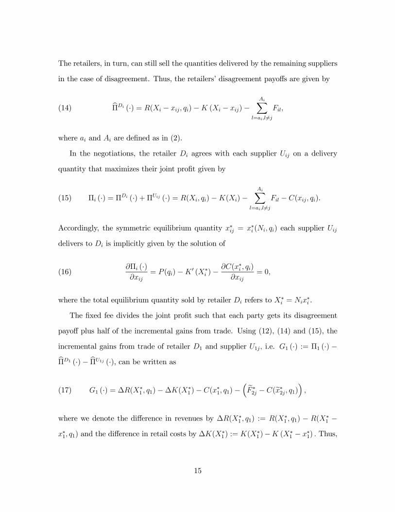
The retailers, in turn, can still sell the quantities delivered by the remaining suppliers
in the case of disagreement. Thus, the retailers�disagreement payo¤s are given by
(14) b�Di (�) = R(Xi � xij; qi)�K (Xi � xij)�AiX
l=ai;l 6=j
Fil;
where ai and Ai are de�ned as in (2).
In the negotiations, the retailer Di agrees with each supplier Uij on a delivery
quantity that maximizes their joint pro�t given by
(15) �i (�) = �Di (�) + �Uij (�) = R(Xi; qi)�K(Xi)�AiX
l=ai;l 6=j
Fil � C(xij; qi).
Accordingly, the symmetric equilibrium quantity x�ij = x�i (Ni; qi) each supplier Uij
delivers to Di is implicitly given by the solution of
(16)@�i (�)@xij
= P (qi)�K 0 (X�i )�
@C(x�i ; qi)
@xij= 0;
where the total equilibrium quantity sold by retailer Di refers to X�i = Nix
�i .
The �xed fee divides the joint pro�t such that each party gets its disagreement
payo¤ plus half of the incremental gains from trade. Using (12), (14) and (15), the
incremental gains from trade of retailer D1 and supplier U1j; i.e. G1 (�) := �1 (�) �b�D1 (�)� b�U1j (�), can be written as(17) G1 (�) = �R(X�
1 ; q1)��K(X�1 )� C(x�1; q1)�
� eF �2j � C(ex�2j; q1)� ;where we denote the di¤erence in revenues by �R(X�
1 ; q1) := R(X�1 ; q1) � R(X�
1 �
x�1; q1) and the di¤erence in retail costs by �K(X�1 ) := K(X
�1 )�K (X�
1 � x�1) : Thus,
15

the symmetric equilibrium �xed fees F �1j = F�1 are chosen such that
(18) �U1j (�) = F �1 � C (x�1; q1) = b�U1j (�) + 12G1 (�) ;implying
(19) F �1 (N1; q1; q2) =�R(X�
1 ; q1)��K(X�1 ) + C(x
�1; q1) +
eF �2j � C(ex�2j; q1)2
;
where eF �2j � C(ex�2j; q1) refers to the value of the supplier�s outside option (see 12).Analogously, the incremental gains from trade of retailer D2 and supplier U2j are
given by
(20)
G2 (�) =
8><>: �R(X�2 ; q2)��K(X�
2 )� C(x�2; q2) if q1 > q2
�R(X�2 ; q2)��K(X�
2 )� C(x�2; q2)�� eF �1j � C(ex�1j; q2)� if q1 = q2
;
where we denote the di¤erence in revenues by �R(X�2 ; q2) := R(X�
2 ; q2) � R(X�2 �
x�2; q2) and the di¤erence in retail costs by �K(X�2 ) := K(X
�2 ) �K (X�
2 � x�2) : The
symmetric equilibrium �xed fees F �2j = F�2 are chosen such that
(21) �U2j (�) = F �2 � C (x�2; q2) = b�U2j (�) + 12G2 (�) ;implying
(22) F �2 (N2; q1; q2) =
8><>:�R(X�
2 ;q2)��K(X�2 )+C(x
�2;q2)
2if q1 > q2
�R(X�2 ;q2)��K(X�
2 )+C(x�2;q2)+
eF �1j�C(ex�1j ;q2)2
if q1 = q2:
It turns out that the suppliers get a larger share of the joint pro�t if they deliver to
the high-quality retailer than if they supply the low-quality retailer.
16

Lemma 2 For given Ni; q1 and q2, there exists a symmetric equilibrium delivery
contract Ti(x�i ; F�i ) 8i; k = 1; 2; i 6= k; where x�i (Ni; qi) maximizes the joint pro�t of
the retailer-supplier pair Di�Uij and the �xed fee F �i (Ni; q1; q2) shares the joint pro�t.
Comparative statics reveal that x�i (Ni; qi) is decreasing (increasing) in Ni (Nk); while
the overall quantity X�i is increasing (decreasing) in Ni (Nk): Furthermore, x
�i (Ni; qi)
is decreasing in qi as long as P 0(qi)� (@2C(x�i ; qi)=@xij@qi) < 0:
Proof. See Appendix A.
Our results reveal that x�i (Ni; qi) is decreasing in Ni due to the convexity of both
production and distribution costs. The increase of x�i (Ni; qi) in Nk is just a mir-
ror image of its decrease in Ni since Nk = N � Ni: Furthermore, x�i (Ni; qi) is de-
creasing in qi as long as the marginal costs of production are su¢ ciently high, i.e.
@2C(x�i ; qi)=@xij@qi > P0(qi).
Using our previous results and taking into account the discontinuity in the equi-
librium �xed fees (see 22), the retailers�reduced pro�t functions are given by
(23) �Di� (�) = R(X�i ; qi)�K(X�
i )�NiF �i :
Correspondingly, the reduced pro�t functions of the suppliers are obtained as
(24) �U1j� (�) =�R(X�
1 ; q1)��K(X�1 )� C(x�1; q1) + eF �2j � C(ex�2j; q1)
2
and
(25) �U2j� (�) =
8><>:�R(X�
2 ;q2)��K(X�2 )�C(x�2;q2)
2if q1 > q2
�R(X�2 ;q2)��K(X�
2 )�C(x�2;q2)+ eF �1j�C(ex�1j ;q2)2
if q1 = q2:
Delivery Choice of Upstream Firms. Taking the retailers�quality requirements
17

q1 and q2 as given, the upstream suppliers decide whether they deliver to retailer
D1 or D2: Any upstream supplier has an outside option if both retailers impose the
same quality standards. Hence, for q1 = q2, half of the suppliers would opt for
retailer D1; while the other half would opt for retailer D2: If, in turn, the retailers�
quality requirements di¤er, i.e. q1 > q2; only the suppliers delivering to the high-
quality retailer D1 have an outside option in the case of negotiation breakdown. This
makes adherence to the higher quality standard more attractive at �rst. However, as
the retailers�marginal costs of distribution are increasing, i.e. K 0(Xi) > 0, not all
upstream �rms decide to supply the high-quality retailer.19
In equilibrium, the upstream �rms are indi¤erent as to which retailer they supply.
Considering q1 > q2 and using the reduced pro�t functions given in (24) and (25), it
must hold in equilibrium that
(26) �U1j�(N1; q1; q2) = �U2j�(N �N1; q2):
Lemma 3 For q1 > q2; equation (26) has a unique solution N�1 (q1; q2); indicating
the equilibrium number of suppliers that deliver to retailer D1: Correspondingly, the
equilibrium number of upstream �rms delivering to D2 is obtained as N�2 (q1; q2) =
N �N�1 (q1; q2):
Proof. See Appendix A.
Denoting x��i (q1; q2) := x�i (N�i (�) ; qi); X��
i (q1; q2) := N�i (�)x��i (q1; q2) and
19Note that we would get a similar e¤ect without considering convex retail costs if there was
imperfect competition in the downstream market. Under imperfect competition, retailers can a¤ect
the market price of their goods by their output decisions. Since the market price is decreasing in the
overall quantity of the good sold in the market, the marginal contribution of the individual suppliers
is decreasing in the number of suppliers delivering to the same retailer.
18

ex��kj(q1; q2) := ex�kj(N�k (�) ; q1; q2); the comparative statics of N�
1 (q1; q2) are as follows:
Lemma 4 For q1 > q2; comparative statics reveal that N�1 (q1; q2) is increasing in q1 if
@C(x��1 ; q1)=@q1 <�P 0(q1)x
��1 � @C(ex��2j ; q1)=@q1 �K 00(X��
1 )(N�1 � 1)x��1 (@x��1 =@q1)
�:
Moreover, N�1 (q1; q2) is decreasing in q2 if @C(x
��2 ; q2)=@q2 < P 0(q2)
�x��2 � ex��2j=2�
�K 00(X��2 )�(N�
2 � 1)x��2 �N�2 ex��2j=2� (@x��2 =@q2) :
Proof. See Appendix A.
Considering q1 > q2; an increase in q1 has two countervailing e¤ects on the
pro�ts of suppliers U1j given in (24). First, it results in a higher gross pro�t,
i.e. @ [�R(X��1 ; q1)��K(X��
1 )� C(x��1 ; q1)] =@q1 > 0: Second, it implies a decline
in the suppliers�outside option, i.e. @h eF �2j(N�
2 ; q1; q2)� C(ex��2j ; q1)i =@q1 < 0: As longas the �rst e¤ect dominates the second, a higher q1 results in a larger number of sup-
pliers delivering to the high-quality retailer and, thus, in fewer suppliers delivering to
D2. This is the case if the production costs are not increasing too strongly in q1 (see
lemma 4).
A rise in q2; however, results in a higher pro�t for the suppliers U2j delivering to
the low-quality retailer D2; i.e. @ [�R(X��2 ; q2)��K(X��
2 )� C(x��2 ; q2)] =@q2 > 0: At
the same time, it improves the outside option of the suppliers U1j delivering to the
high-quality retailer D1: Again, if the �rst e¤ect dominates the second, a higher q2
leads to a lower number of suppliers delivering to the high-quality retailer, implying
a larger number of suppliers opting for the low-quality retailer. This holds if the
production costs are not increasing too strongly in q2 (see lemma 4).
19

Private Quality Standards
In this section, we analyze the retailers�choice of quality requirements. Both retailers
set their private quality standards so as to maximize their respective pro�t functions.
Denoting F ��i := F �i (N�i ; q1; q2), the equilibrium quality requirements are, thus, given
by
q�i : = argmaxqi
�Di�� (�)(27)
with : �Di�� (�) = [R (X��i ; qi)�K(X��
i )�N�i F
��i ] :
Equilibrium Analysis. In our setting, there exists no symmetric equilibrium in the
retailers�quality requirements.20
Considering q1 = q2; the upstream �rms can deliver to both retailers when comply-
ing with the respective quality standard. Thus, all suppliers have an outside option
in the case of disagreement with their initially chosen retailer.
If retailer D1 increases its quality requirements by an arbitrarily small amount to
q1 = q2 + ", two e¤ects emerge: The suppliers U2j delivering to D2 lose their outside
option and the outside option of the suppliers U1j becomes less valuable. The reason
for the latter is that the suppliers still incur the production costs associated with q1
when switching to D2, while they are only rewarded for supplying q2: As long as "
is su¢ ciently small, the �rst e¤ect dominates the second. Accordingly, delivery to
D1 becomes more attractive, resulting in a higher N�1 . A larger number of suppliers
delivering to the high-quality retailer, in turn, induces the following trade-o¤: First,
the higher N�1 results in a lower quantity delivered by each supplier (see lemma 2),
20If the suppliers generally have no possibility to switch their delivery to the other retailer, there
will be a symmetric equilibrium in qualities (see von Schlippenbach and Teichmann 2011).
20

such that the joint pro�t of retailer D1 and any of its suppliers is increasing. Second,
a higher N�1 implies a lower N
�2 ; which improves the disagreement payo¤ of suppliers
U1j: In other words, the marginal contribution of the switching supplier eU2j to thejoint pro�t with the retailer D2 is increasing if N�
2 is decreasing (lemma 1). As the
�rst e¤ect dominates the second, the retailers have an incentive to deviate from the
symmetric candidate equilibrium.
Proposition 1 There exists no symmetric equilibrium in the retailers� quality re-
quirements as the retailers always have an incentive to deviate from the symmetric
candidate equilibrium.
Proof. See Appendix A.
To ensure the existence of an asymmetric equilibrium in the retailers� quality
choice, the marginal costs of production need to be su¢ ciently convex in quality and
quantity as this eliminates the incentive for retailers to leapfrog each other. Consistent
with our above assumptions, we apply the following inverse demand functions P (qi) =pqi; production-cost functions C(xij; qi) = q3i x
2ij=3 and retail-cost functions K(Xi) =
X2i for i = 1; 2 to illustrate our results numerically.
21
Result 1 Numerical analysis shows that there exists an asymmetric equilibrium in
the retailers�quality choice, i.e. q�1 > q�2; if the suppliers�production costs are su¢ -
ciently convex in quality and quantity.
< Insert �gure 1 >
21Numerical results for the equilibrium quantities, �xed fees and the number of suppliers delivering
to Di can be found in Appendix B.
21

Considering a relatively low value of q�2, the best response of retailer D1 is to raise
its quality requirements above q�2 (�gure 1, upper panel). As described above, an
increase in q1, starting from q1 = q�2, leads to more suppliers delivering to D1 and,
thus, to a larger joint pro�t of the retailer D1 and any of its suppliers U1j due to the
lower quantity delivered by each supplier. However, for very high values of q1, the
rise in the quality-related production costs dominates the favorable quantity e¤ect.
This puts limits to the rise in q1:
Taking now a relatively high quality standard q�1 as given, the best response of
retailer D2 is to considerably undercut the quality requirements of D1 (�gure 1, lower
panel). If q2 drops just below q�1; i.e. q2 = q�1 � "; the suppliers U2j lose their
outside option: This makes delivery to the now low-quality retailer less attractive
than supplying the high-quality retailer. Furthermore, a lower number of upstream
�rms supplying the same retailer leads to a larger quantity to be delivered by each of
these suppliers (lemma 2). This results in a disproportionately strong increase in the
production costs since these are strictly convex in quantity. Retailer D2; therefore,
has an incentive to considerably undercut q�1: First, lower quality requirements result
in lower quality-related production costs. Second, a lower q2 relative to q�1 reduces the
outside option of suppliers U1j; making delivery to D1 less attractive. Note, however,
that the retailer D2 has no incentive to decrease its quality requirements unlimitedly
since the reduced quality implies lower prices in the �nal consumer market and, thus,
decreases the retailer�s revenue.
Result 2 Numerical analysis further reveals that the quality requirements q�1 and q�2
as well as the di¤erence q�1 � q�2 are increasing in N .
< Insert �gure 2 >
22

The higher N; the more suppliers decide to deliver to the high-quality retailer D1
since N�1 � N=2: This results in a decrease in the quantity delivered by each supplier
U1j (lemma 2), leading to a reduction in the quantity-related production costs. On this
basis, the retailer D1 is able to increase its quality requirements in order to strengthen
its bargaining position by weakening the suppliers�outside option. A higher q�1, in
turn, enables the retailer D2 to increase its quality requirements q�2 as well, resulting
in a higher joint pro�t with the suppliers. Due to the disproportionate increase of N�1
in N; a relatively higher quantity is produced by each supplier delivering to the low-
quality retailer. This implies that the quality requirement of the low-quality retailer is
less increasing in N than the quality requirement of the high-quality retailer. Hence,
the spread between q�1 and q�2 is increasing in N (�gure 2).
Under the assumption of perfect competition, the retailers�choice of private qual-
ity standards is not a¤ected by downstream market features. In other words, the
retailers do not di¤erentiate in quality in order to soften the competition in �nal con-
sumer markets. The only reason to di¤erentiate in quality is driven by the retailers�
incentive to improve their bargaining position vis-à-vis their suppliers and, thus, to
gain buyer power in the intermediate goods market. We �nd that the joint pro�t of
the low-quality retailer with any of its suppliers is smaller than the respective joint
pro�t obtained by the high-quality retailer as long as the quality requirements have a
stronger impact on the retailers�revenue than on production costs. Referring to the
above-described outside-option e¤ect, the low-quality retailer gets a larger share of a
smaller pie, while the high-quality retailer gets a smaller share of a larger pie. Note
that the suppliers make the same pro�t in equilibrium, no matter which retailer they
supply.
The implementation of private quality standards induces ine¢ ciencies in the up-
stream production. Due to the convexity of the production and distribution costs, the
23

industry pro�t is maximized if both retailers implement the same quality requirements
and the suppliers split equally between the retailers.22 However, from proposition 1
we know that there is no symmetric equilibrium in the retailers�pro�t-maximizing
quality choice. Hence, we get:
Proposition 2 The strategic use of private quality standards by retailers results in an
ine¢ cient production structure. The ine¢ ciency rises in N since the spread between
q�1 and q�2 is increasing in N .
23
Extension: Imperfect Competition
In the following, we relax the assumption of perfect competition to account for the
highly concentrated retail sector in many European countries (Dobson, Waterson
and Davies 2003; OECD 2006). Leaving the underlying bargaining mechanism un-
changed, we now assume that the retailers are horizontally di¤erentiated and compete
in quantities in the �nal consumer market. This allows us to analyze the impact of
downstream market features on the retailers�quality choice. We consider a represen-
tative consumer with the utility function24
(28) U(X1; X2) =2Xi=1
pqiXi �
1
2
2Xi=1
X2i + 2�X1X2
!�
2Xi=1
PiXi, 8i = 1; 2;
22Note that under our assumptions the quality level that maximizes industry pro�t equals the
socially optimal quality level.
23The negative impact of private quality standards on the production structure can be limited
by enforcing a binding public MQS (see Appendix C).
24This utility function is based on the symmetric, additively separable utility function proposed
by Dixit and Stiglitz (1977).
24

where � 2 [0; 1) indicates the degree of substitutability between the retailers 1 and
2: The closer � approaches one, the more the retailers are substitutable. The dif-
ferentiation is based on parameters associated with the retail outlet, such as store
atmosphere, product range and location. Di¤erentiating (28) with respect to Xi; the
inverse demand functions refer to Pi (qi; Xi; Xk) = max�pqi �Xi � �Xk; 0
; with
i; k = 1; 2; i 6= k: That is, the inverse demand functions are twice continuously dif-
ferentiable in qi with @Pi (qi; �) =@qi > 0 and @2Pi (qi; �) =@q2i < 0 for Pi (qi; �) > 0:
The production-cost functions and the retail-cost functions remain the same as under
perfect competition with C(xij; qi) = q3i x2ij=3 and K(Xi) = X2
i . Moreover, we still
assume that q1 � q2.
Equilibrium Analysis. Solving the third stage of the game, we get the equilib-
rium quantities ex�kj(Xi; q1; q2) and x�i (Ni; q1; q2) as well as the �xed fees eF �kj(Xi; q1; q2)
and F �i (Ni; q1; q2): In the second stage of the game, we obtainN�i ; which leads us to the
reduced forms x��i := x�i (N
�i ; q1; q2); X
��i := N
�ix��i and F
��i := F
�i (N
�i ; q1; q2):
25 Finally,
in the �rst stage, we analyze the equilibrium quality choice of the retailers. There
is an asymmetric equilibrium in the retailers�quality requirements as in the case of
perfect competition (�gure 3). The reasoning is as before: Retailer D1 strengthens
its quality requirements to attract more suppliers and, at the same time, to improve
its bargaining position in the negotiations with the suppliers. The best response of
retailer D2 is to reduce its quality requirements. However, the prevalence of imperfect
competition gives rise to an additional e¤ect as the quantities sold by the retailers
now a¤ect the overall market outcome. By increasing its quality requirements, D1
commits itself to sell a higher quantity to �nal consumers. The reason is that the
retailer attracts more suppliers by increasing q1; resulting in a larger X��1 (lemma 2).
25Numerical results for the equilibrium quantities, �xed fees and the number of suppliers delivering
to Di can be found in Appendix B.
25

As quantities are strategic substitutes in our setting, the best response of the com-
petitor D2 is to decrease its quantity in the �nal consumer market. D2 is able to do so
by reducing its quality requirements. This e¤ect becomes less pronounced the more
di¤erentiated the retailers are and, thus, the softer downstream competition. This
also implies that the ine¢ ciency induced by the retailers�private standard setting is
decreasing in the degree of retail di¤erentiation.
< Insert �gure 3 >
Result 3 The results obtained under perfect competition in the downstream market
do not qualitatively change when imperfect downstream competition is considered.
Minimum Quality Standard. The ine¢ ciency in upstream production induced
by the retailers�quality choice under imperfect competition can be limited by enforc-
ing a binding public MQS. Under such a MQS, the retailer with the lower quality
requirements cannot unrestrictedly reduce its quality standard in response to increas-
ing quality requirements of the other retailer. As a consequence, the high-quality
retailer has less incentive to increase its quality standard, such that the spread in the
high and low quality requirements is reduced.26
26Under perfect competition, the low-quality retailer also increases its quality requirements when
a public MQS is enforced. In contrast to the case of imperfect competition, the best response of the
high-quality retailer is to increase its quality requirements as well. Overall, the �rst e¤ect dominates
the second, such that a public MQS also mitigates the unfavorable e¤ects of private quality standards
under perfect competition (see Appendix C).
26

Conclusion
Our analysis indicates that retailers use private quality standards to improve their
buyer power in the food supply chain, leading to ine¢ cient production structures in
the upstream market. The ine¢ ciency in the upstream production is increasing in
both the number of upstream suppliers and, in the case of imperfect competition,
the degree of substitutability among retailers. We �nd that the implementation of a
binding public MQS mitigates the unfavorable e¤ects from the retailers�strategic use
of quality standards.
These results hold for both perfect and imperfect competition in the downstream
retail market. However, our �ndings are limited to production costs that are su¢ -
ciently convex in quality and quantity. Moreover, it is required that suppliers cannot
easily change their production process to comply with di¤erent quality requirements.
This refers mainly to industries where producers face high quality-related production
costs and are locked in their production processes in the short-term, such as in the
production of fruits and vegetables.
References
Allain, M.-L. 2002. The Balance of Power between Producers and Retailers: A Dif-
ferentiation Model. Louvain Economic Review 68(3): 359-370.
Balsevich, J., A. Berdegué, L. Flores, D. Mainville and T. Reardon. 2003. Su-
permarkets and Produce Quality and Safety Standards in Latin America. American
Journal of Agricultural Economics 85(5): 1147-1154.
Bazoche, P., E. Giraud-Héraud and L.-G. Soler. 2005. Premium Private Labels,
Supply Contracts, Market Segmentation, and Spot Prices. Journal of Agricultural
27

and Food Industrial Organization 3: Article 7.
Bernard, J. C. and D. J. Bernard. 2009. What Is It About Organic Milk? An
Experimental Analysis. American Journal of Agricultural Economics 91(3): 826-836.
Berto Villas-Boas, S. 2007. Vertical Relationships between Manufacturers and
Retailers: Inference with Limited Data. Review of Economic Studies 74(2): 625-652.
Binmore, K., A. Rubinstein and A.Wolinsky. 1986. The Nash Bargaining Solution
in Economic Modelling. Rand Journal of Economics 17(2): 176-188.
Boselie, D., S. Henson and D. Weatherspoon. 2003. Supermarket Procurement
Practices in Developing Countries: Rede�ning the Roles of the Public and Private
Sectors. American Journal of Agricultural Economics 85(5): 1155-1161.
Bonnet, C. and P. Dubois. 2010. Inference on Vertical Contracts between Manu-
facturers and Retailers Allowing for Nonlinear Pricing and Resale Price Maintenance.
RAND Journal of Economics 41(1): 139-164.
Bougherara, D. and P. Combris. 2009. Eco-Labelled Food Products: What are
Consumers Paying for? European Review of Agricultural Economics 36(3): 321-341.
Brooks, K. and J. L. Lusk. 2010. Stated and Revealed Preferences for Organic and
Cloned Milk: Combining Choice Experiment and Scanner Data. American Journal
of Agricultural Economics 92(4): 1229-1241.
Caprice, S. 2006. Multilateral Vertical Contracting with an Alternative Supply:
The Welfare E¤ects of a Ban on Price Discrimination. Review of Industrial Organi-
zation 28(1): 63-80.
Chambolle, C. and S. Berto Villas-Boas. 2010. Buyer Power through Producers�
Di¤erentiation. mimeo.
Codron, J.-M., E. Giraud-Héraud and L.-G. Soler. 2005. Minimum Quality Stan-
dards, Premium Private Labels, and European Meat and Fresh Produce Retailing.
Food Policy 30(3): 270-283.
28

Crampes, C. and A. Hollander. 1995. Duopoly and Quality Standards. European
Economic Review 39(1): 71-82.
Dixit, A. K. and J. E. Stiglitz. 1977. Monopolistic Competition and Optimum
Product Diversity. American Economic Review 67(3): 297-308.
Dobson, P. W., M. Waterson and S. W. Davies. 2003. The Patterns and Implica-
tions of Increasing Concentration in European Food Retailing. Journal of Agricultural
Economics 54(1): 111-125.
Gal-Or, E. 1985. Di¤erentiated Industries without Entry Barriers. Journal of
Economic Theory 37(2): 310-339.
Gal-Or, E. 1987. Strategic and Non-Strategic Di¤erentiation. Canadian Journal
of Economics 20(2): 340-356.
Gao, Z. and T. C. Schroeder. 2009. E¤ects of Label Information on Consumer
Willingness-to-Pay for Food Attributes. American Journal of Agricultural Economics
91(3): 795-809.
García Martinez, M. and N. Poole. 2004. The Development of Private Fresh Pro-
duce Safety Standards: Implications for Developing Mediterranean Exporting Coun-
tries. Food Policy 29(3): 229-255.
Gil, J. M., A. Gracia and M. Sánchez. 2000. Market Segmentation and Will-
ingness to Pay for Organic Products in Spain. International Food and Agribusiness
Management Review 3(2): 207-226.
Giraud-Héraud, E., L. Rouached and L.-G. Soler. 2006. Private Labels and Public
Quality Standards: How Can Consumer Trust Be Restored after the Mad Cow Crisis?
Quantitative Marketing and Economics 4(1): 31-55.
Giraud-Héraud, E., H. Hammoudi and L.-G. Soler. 2006. Food Safety, Liability
and Collective Norms. Cahiers du Laboratoire d�Econométrie de l�Ecole Polytech-
nique, No. 2006-06.
29

Giraud-Héraud, E., H. Hammoudi, R. Ho¤mann and L.-G. Soler. 2008. Vertical
Relationships and Safety Standards in the Food Marketing Chain. Working Paper
ALISS 2008-07.
Hammoudi, A., R. Ho¤mann and Y. Surry. 2009. Food Safety Standards and
Agri-Food Supply Chains: An Introductory Overview. European Review of Agricul-
tural Economics 36(4): 469-478.
Horn, H. and A. Wolinsky. 1988. Bilateral Monopolies and Incentives for Merger.
RAND Journal of Economics 19(3): 408-419.
Inderst, R. and N. Mazzarotto. 2008. Buyer Power in Distribution. In: Collins,
W. D. (ed.). ABA Antitrust Section Handbook, Issues in Competition Law and Policy.
Volume III: 1953-1978.
Inderst, R. and G. Sha¤er. 2008. Buyer Power in Merger Control. In: Collins, W.
D. (ed.). ABA Antitrust Section Handbook, Issues in Competition Law and Policy.
Volume II: 1611-1636.
Jang, J. and F. Olson. 2010. The Role of Product Di¤erentiation for Contract
Choice in the Agro-Food Sector. European Review of Agricultural Economics 37(2):
251-273.
Kalai, E. and M. Smorodinsky. 1975. Other Solutions to Nash�s Bargaining
Problem. Econometrica 43(3): 513-518.
Kanter, C., K. D. Messer and H. M. Kaiser. 2009. Does Production Labeling
Stigmatize Conventional Milk? American Journal of Agricultural Economics 91(4):
1097-1109.
Katz, M. L. 1987. The Welfare E¤ects of Third Degree Price Discrimination in
Intermediate Goods Markets. American Economic Review 77(1): 154-167.
Lutz, S., T. P. Lyon and J. W. Maxwell. 2000. Quality Leadership when Regula-
tory Standards are Forthcoming. Journal of Industrial Economics 48(3): 331-348.
30

Marcoul, P. and L. Veyssiere. 2010. A Financial Contracting Approach to the
Role of Supermarkets in Farmers�Credit Access. American Journal of Agricultural
Economics 92(4): 1051-1064.
Marks & Spencer. 2010. How We Do Business Report 2010. Marks and Spencer
Group plc, United Kingdom.
Mayen, C. D., J. V. Balagtas and C. E. Alexander. 2010. Technology Adaption
and Technical E¢ ciency: Organic and Conventional Dairy Farms in The United
States. American Journal of Agricultural Economics 92(1): 181-195.
McAfee, R. P. and M. Schwartz. 1995. The Non-Existence of Pairwise-Proof
Equilibrium. Economics Letters 49(3): 251-259.
McAfee, R. P. and M. Schwartz. 1994. Opportunism in Multilateral Vertical
Contracting: Nondiscrimination, Exclusivity, and Uniformity. American Economic
Review 84(1): 210-230.
McCluskey, J. J. and J. A. Winfree. 2009. Pre-Empting Public Regulation with
Private Food Quality Standards. European Review of Agricultural Economics 36(4):
525-539.
Motta, M. 1993. Endogenous Quality Choice: Price vs. Quantity Competition.
Journal of Industrial Economics 41(2): 113-131.
Nash, J. 1953. Two-Person Cooperative Games. Econometrica 21(1): 128-140.
OECD. 2007. Private Standard Schemes and Developing Country Access to Global
Value Chains: Challenges and Opportunities Emerging from Four Case Studies.
OECD. 2006. Final Report on Private Standards and the Shaping of the Agro-food
System.
O�Brien, D. P. and G. Sha¤er. 1992. Vertical Control with Bilateral Contracts.
RAND Journal of Economics 23(3): 299-308.
PAN Europe. 2008. Supermarkets Fact Sheet.
31

Available at: http://www.pan-europe.info/Resources/Factsheets/Supermarkets.pdf
(accessed March, 2 2011).
Rey, P. and T. Vergé. 2008. Economics of Vertical Restraints. In: Buccirossi, P.
(ed.). Handbook of Antitrust Economics. The MIT Press: 353-390.
Ronnen, U. 1991. Minimum Quality Standards, Fixed Costs, and Competition.
RAND Journal of Economics 22(4): 490-504.
Rubinstein, A. 1982. Perfect Equilibrium in a Bargaining Model. Econometrica
50(1): 97-109.
She¤man, D. T. and P. T. Spiller. 1992. Buyers�Strategies, Entry Barriers, and
Competition. Economic Inquiry 30(3): 418-436.
Valletti, T. M. 2000. Minimum Quality Standards under Cournot Competition.
Journal of Regulatory Economics 18(3): 235-245.
Vandemoortele, T. 2011. When are Private Standards more Stringent than Public
Standards? mimeo.
von Schlippenbach, V. and I. Teichmann. 2011. The Strategic Use of Private
Quality Standards in Food Supply Chains. DIW Discussion Paper 1120. German
Institute for Economic Research (DIW Berlin).
Wal-Mart. 2008a. Wal-Mart Becomes First Nationwide U.S. Grocer To Adopt
Global Food Safety Initiative Standards. Available at:
http://walmartstores.com/pressroom/news/7918.aspx (accessed March, 8 2011).
Wal-Mart. 2008b. Wal-Mart is Taking the Lead on Sustainable Packaging.
Available at: http://walmartstores.com/pressroom/factsheets/ (accessed March, 2
2011).
Wal-Mart. 2011. China Sustainability Summit: Fact Sheet. Available at:
http://walmartstores.com/pressroom/factsheets/ (accessed March, 2 2011).
32

Appendix A
Proof of lemma 1. To determine the comparative statics of ex�ij (�), we apply theimplicit-function theorem and use
e�i (�) = e�Di (�) + e�eUij (�) = R(Xi + exij; qi)�K(Xi + exij)� AiXl=ai
Fil � C (exij; qk)with :
8><>: ai = 1; Ai = N1 for i = 1
ai = N1 + 1; Ai = N for i = 2:
Since
(29) @2e�i (�) =@ex2ij = � �K 00(Xi + ex�ij (�)) + @2C(ex�ij (�) ; qk)=@ex2ij� < 0;the comparative statics of ex�ij (�) are given by sign
�@ex�ij (�) =@�� =
sign�@2e�i (�) =@exij@�� for � = qi; qk; Ni. Thus, it holds that
sign
�@ex�ij (�)@qk
�< 0 since
@2e�i (�)@exij@qk = �@
2C(ex�ij (�) ; qk)@exij@qk < 0;(30)
sign
�@ex�ij (�)@qi
�> 0 since
@2e�i (�)@exij@qi = P 0(qi) > 0;(31)
sign
�@ex�ij (�)@Ni
�< 0 since
@2e�i (�)@exij@Ni = �K 00(Xi + ex�ij)ex�ij < 0:(32)
Proof of lemma 2. To determine the comparative statics of x�i (�), we apply the
implicit-function theorem. Denoting H(Ni; x�i (Ni; qi)) = 0 the �rst-order condition
given in (16) and using @H(�)=@xij = ��NiK
00(X�i (�)) + @2C(x�i (�) ; qi)=@x2ij
�< 0,
33

we get
sign
�@x�i (�)@Ni
�= sign
�@H(Ni; x
�i (�))
@Ni
�= �K 00(X�
i (�))x�i (�) < 0 ;(33)
sign
�@x�i (�)@Nk
�= sign
�@H(Ni; x
�i (�))
@Nk
�= K 00(X�
i (�))x�i (�) > 0:(34)
Considering the overall quantity, we have
@X�i (�)@Ni
= x�i (�)�1� NiK
00(X�i (�))
NiK 00(X�i (�)) + @2C(x�i (�) ; qi)=@x2ij
�> 0:
Correspondingly, it holds that @X�i (�) =@Nk < 0: Furthermore, we have
sign
�@x�i (�)@qi
�= sign
�@H(Ni; x
�i (�))
@qi
�= P 0(qi)�
@2C(x�i (�) ; qi)@xij@qi
? 0;(35)
sign
�@x�i (�)@qk
�= 0 since
@H(Ni; x�i (�))
@qk= 0:(36)
Proof of lemma 3. To prove the existence of N�1 (�) ; we �rst show that the
di¤erence in the upstream �rms� pro�ts, ��U (�) = �U1j�(N1; q1; q2) � �U2j�(N �
N1; q2) is monotonically decreasing in N1: That is, we show that @��U (�) =@N1 < 0,
i.e.
(37)@��U (�)@N1
= �12[�1 + �2 � �3] < 0
34

with
�1 = (K 0(X�1 (�))�K 0(X�
1 (�)� x�1 (�)))�x�1 (�) + (N1 � 1)
@x�1 (�)@N1
�;
�2 =1
2
�K 0(X�
2 (�) + ex�2j (�))�K 0 (X�2 (�))
���x�2 (�) + (N �N1)
@x�2 (�)@N1
�;
�3 = (K 0(X�2 (�))�K 0 (X�
2 (�)� x�2 (�)))��x�2 (�) + (N �N1 � 1)
@x�2 (�)@N1
�:
From lemma 2, we immediately get x�1 (�)+ (N1�1) (@x�1 (�) =@N1) > 0; which implies
�1 > 0: Analogously, we obtain
(38)��x�2 (�) + (N �N1 � 1)
@x�2 (�)@N1
�<
��x�2 (�) + (N �N1)
@x�2 (�)@N1
�< 0:
It remains to show that �2 � �3 > 0; which holds as long as
(39)1
2
�K 0(X�
2 (�) + ex�2j (�))�K 0 (X�2 (�))
�� (K 0(X�
2 (�))�K 0 (X�2 (�)� x�2 (�))) < 0:
Since ex�2j (�) < x�2 (�) due to the comparison of (7) and (16), we can consider ex�2j (�) =x�2 (�) and get that (39) is obviously ful�lled for K 000(�) = 0. However, condition (39)
is likewise ful�lled if K 00(�) is not too large, i.e. the retailers�costs are not too convex
in quantity.
Second, we show that �U1j�(1; �) > �U2j�(N � 1; �). Considering q1 = q2 + " and
N1 = N2 = 1 for given N = 2, we get �U1j�(1; �) > �U2j�(1; �) as supplier U1j has a
strictly positive outside option in contrast to supplier U2j: �U2j�(N2; �) is decreasing
in N2 since the marginal contribution of any individual supplier is the lower the
more suppliers deliver to the same retailer. Accordingly, it holds that �U1j�(1; �) >
�U2j�(N � 1; �) for any N � 2: For N su¢ ciently large, it holds analogously that
�U1j�(N � 1; �) < �U2j�(1; �): Thus, there exists an equilibrium N�1 (�) :
35
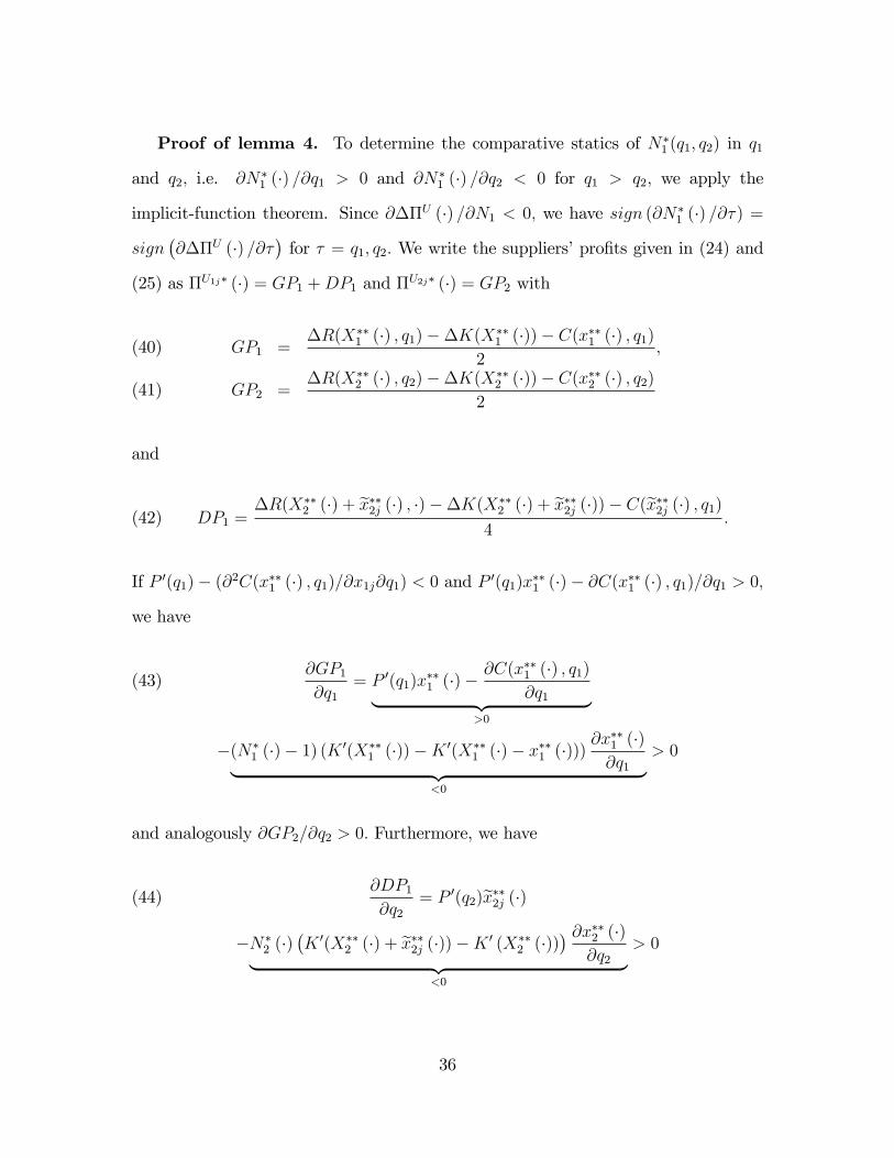
Proof of lemma 4. To determine the comparative statics of N�1 (q1; q2) in q1
and q2; i.e. @N�1 (�) =@q1 > 0 and @N�
1 (�) =@q2 < 0 for q1 > q2; we apply the
implicit-function theorem. Since @��U (�) =@N1 < 0; we have sign (@N�1 (�) =@�) =
sign�@��U (�) =@�
�for � = q1; q2: We write the suppliers�pro�ts given in (24) and
(25) as �U1j� (�) = GP1 +DP1 and �U2j� (�) = GP2 with
GP1 =�R(X��
1 (�) ; q1)��K(X��1 (�))� C(x��1 (�) ; q1)
2;(40)
GP2 =�R(X��
2 (�) ; q2)��K(X��2 (�))� C(x��2 (�) ; q2)
2(41)
and
(42) DP1 =�R(X��
2 (�) + ex��2j (�) ; �)��K(X��2 (�) + ex��2j (�))� C(ex��2j (�) ; q1)
4:
If P 0(q1)� (@2C(x��1 (�) ; q1)=@x1j@q1) < 0 and P 0(q1)x��1 (�)� @C(x��1 (�) ; q1)=@q1 > 0;
we have
@GP1@q1
= P 0(q1)x��1 (�)�
@C(x��1 (�) ; q1)@q1| {z }
>0
(43)
�(N�1 (�)� 1) (K 0(X��
1 (�))�K 0(X��1 (�)� x��1 (�)))
@x��1 (�)@q1| {z }
<0
> 0
and analogously @GP2=@q2 > 0: Furthermore, we have
@DP1@q2
= P 0(q2)ex��2j (�)(44)
�N�2 (�)
�K 0(X��
2 (�) + ex��2j (�))�K 0 (X��2 (�))
� @x��2 (�)@q2| {z }
<0
> 0
36

and
(45)@DP1@q1
= �@C(ex��2j (�) ; q1)
@q1< 0:
Turning to the comparative static results, we get
(46) sign
�@N�
1 (�)@q1
�= sign
�@��U (�)@q1
�= sign
�@GP1@q1
+@DP1@q1
�> 0
and
(47) sign
�@N�
1 (�)@q2
�= sign
�@��U (�)@q2
�= sign
�@DP1@q2
� @GP2@q2
�< 0:
Condition (46) is ful�lled if
@C(x��1 (�) ; q1)@q1
< P 0(q1)x��1 (�)�
@C(ex��2j (�) ; q1)@q1
(48)
�(N�1 (�)� 1) (K 0(X��
1 (�))�K 0(X��1 (�)� x��1 (�)))
@x��1 (�)@q1
:
Applying the �rst-order Taylor approximation, (48) can be rewritten as
@C(x��1 (�) ; q1)@q1
< P 0(q1)x��1 (�)�
@C(ex��2j (�) ; q1)@q1
(49)
�K 00(X��1 (�))(N�
1 (�)� 1)x��1 (�)@x��1 (�)@q1
:
Likewise, condition (47) is ful�lled if
@C(x��2 (�) ; q2)@q2
< P 0(q2)(x��2 (�)� ex��2j (�) =2)(50)
�2(N�
2 (�)� 1)�K 0(X��2 (�))�N�
2 (�)�K 0(X��2 (�) + ex��2j (�))
2
@x��2 (�)@q2
;
37

with : �K 0(X��2 (�)) = K 0(X��
2 (�))�K 0 (X��2 (�)� x��2 (�))
and : �K 0(X��2 (�) + ex��2j (�)) = K 0(X��
2 (�) + ex��2j (�))�K 0 (X��2 (�)) :
Applying the �rst-order Taylor approximation, (50) can be rewritten as
@C(x��2 (�) ; q2)@q2
< P 0(q2)2x��2 (�)� ex��2j (�)
2(51)
�K 00(X��2 (�))
�(N�
2 (�)� 1)x��2 (�)�N�2 (�)2
ex��2j (�)� @x��2 (�)@q2:
Proof of proposition 1. To prove that there exists no symmetric equilibrium in
the retailers�quality choice, we show that the retailers always have an incentive to
deviate from the symmetric candidate equilibrium. We, thus, compare the pro�t of
retailer D1 in the case of equal quality requirements, i.e. q1 = q2; with its pro�t in the
case of q1 = q2+": If retailer D1 exceeds the quality requirements of retailer D2 by an
arbitrarily small amount "; delivery to D1 becomes more attractive as the suppliers
delivering toD2 lose their outside option. Accordingly, N�1 (�) is increasing. Neglecting
any quality e¤ect from the small increase in q1; we show that @�D1�� (�) =@N1 > 0 in
order to prove proposition 1.
First, we show that the overall pro�t of retailer D1 and all its N�1 (�) suppliers
U1j; i.e. (�) = P (q1)X��1 (�) �K(X��
1 (�)) � N�1 (�)C(x��1 (�) ; q1); is increasing in N1:
Applying the envelope theorem, we have
(52)@(�)@N1
= (P (q1)�K 0(X��1 (�)))x��1 (�)� C(x��1 (�) ; q1):
By using (16), (52) can be rewritten as
(53)@(�)@N1
=@C(x��1 (�) ; q1)
@x1jx��1 (�)� C(x��1 (�) ; q1) > 0:
38

Condition (53) is ful�lled due to the assumed convexity of production costs C(x1j; q1).
Second, denote �Uij�� (�) := �Uij� (N�i (�) ; �). Using (�) = �D1��(�)+N�
1�U1j�� (�),
we compare the overall pro�t (�) for q1 = q2 with N1 := N�1 (q2; q2); x1 := x
��1 (q2; q2)
and X1 := X��1 (q2; q2) to (�) for q1 = q2 + " with N1 := N�
1 (q2 + "; q2); x1 :=
x��1 (q2 + "; q2); X1 := X��1 (q2 + "; q2); ex2j := ex��2j(q2 + "; q2) and eF 2j := eF ��2j (q2 + "; q2):
Denoting�D1 := �D1��(N1; �), �D1:= �D1��(N1; �); �U1j := �U1j��(N1; �) and�
U1j:=
�U1j��(N1; �), we write (�) = �D1+N1
��U1j � �U1j
�+�N1 �N1
��U1j . Evaluating
the di¤erence �(�) = (�)� (�), we get
(54) �(�) = �D1 � �D1 +hN1
��U1j � �U1j
�+�N1 �N1
��U1ji;
which can be rewritten as
(55) �D1 � �D1 = �(�)�
hN1
��U1j � �U1j
�+�N1 �N1
��U1ji:
Note that �U1j��U1j < 0. This is due to the fact that all the suppliers have an outside
option if q1 = q2: If, instead, q1 increases by " to q2 + "; the suppliers delivering to
D2 lose their outside option, implying a lower pro�t �U2j�� (�) : This implies that
more suppliers decide to deliver to D1; resulting in a higher pro�t of those suppliers
delivering to D2: As, in equilibrium, the pro�ts of the suppliers delivering to D1 and
D2 are equal, the pro�t �U1j�� (�) must decrease in N�1 (�) ; i.e. �
U1j � �U1j < 0:
Furthermore, from (53) we know that �(�) > 0. Accordingly, it remains to show
that �(�) ��N1 �N1
��U1j: Using �rst-order Taylor approximation, we rewrite
�(�) = N1(P (q1)x1 � C(x1; q1)) � K(X1) � [N1(P (q1)x1 � C(x1; q1))�K(X1)]
as �e(�) = �N1 �N1
� �P (q1)x1 � C(x1; q1)�K 0(X1)x1
�:
39

Thus, we show that
�N1 �N1
� �P (q1)x1 � C(x1; q1)�K 0(X1)x1
�>(56) �
N1 �N1
�2
�P (q1)x1 �K 0(X1)x1 � C(x1; q1) + eF 2j � C(ex2j; qi)� ;
which simpli�es to
(57) P (q1)x1 � C(x1; q1)�K 0(X1)x1 > P (q2)ex2j � C(ex2j; q1)�K 0(X2 + ex2j)ex2j:The left-hand side of inequality (57) is equal or larger than the incremental gains
from trade between D1 and U1j given in (17). The right-hand side of (57) equals
the o¤-equilibrium incremental gains from trade as given in (9). Therefore, we can
conclude that (57) is always ful�lled due to the properties of the bargaining solution.
Accordingly, we have �(�)�hN1
��U1j � �U1j
�+�N1 �N1
��U1ji> 0, such that
�D1 � �D1 cannot be negative.
Appendix B
Numerical Results under Perfect Competition. Plugging the functions P (qi) =pqi, C(xij; qi) = q3i x
2ij=3 and K(Xi) = X
2i into equations (19) and (22), the equilib-
rium �xed fees F �1 (�) and F �2 (�) for q1 � q2 are given by
(58) F �1 (�) =pq1x
�1(�)� (2N1 � 1)x�1(�)2 +
q313x�1(�)2 + eF �2j (�)� q31
3ex�2j(�)2
2;
40
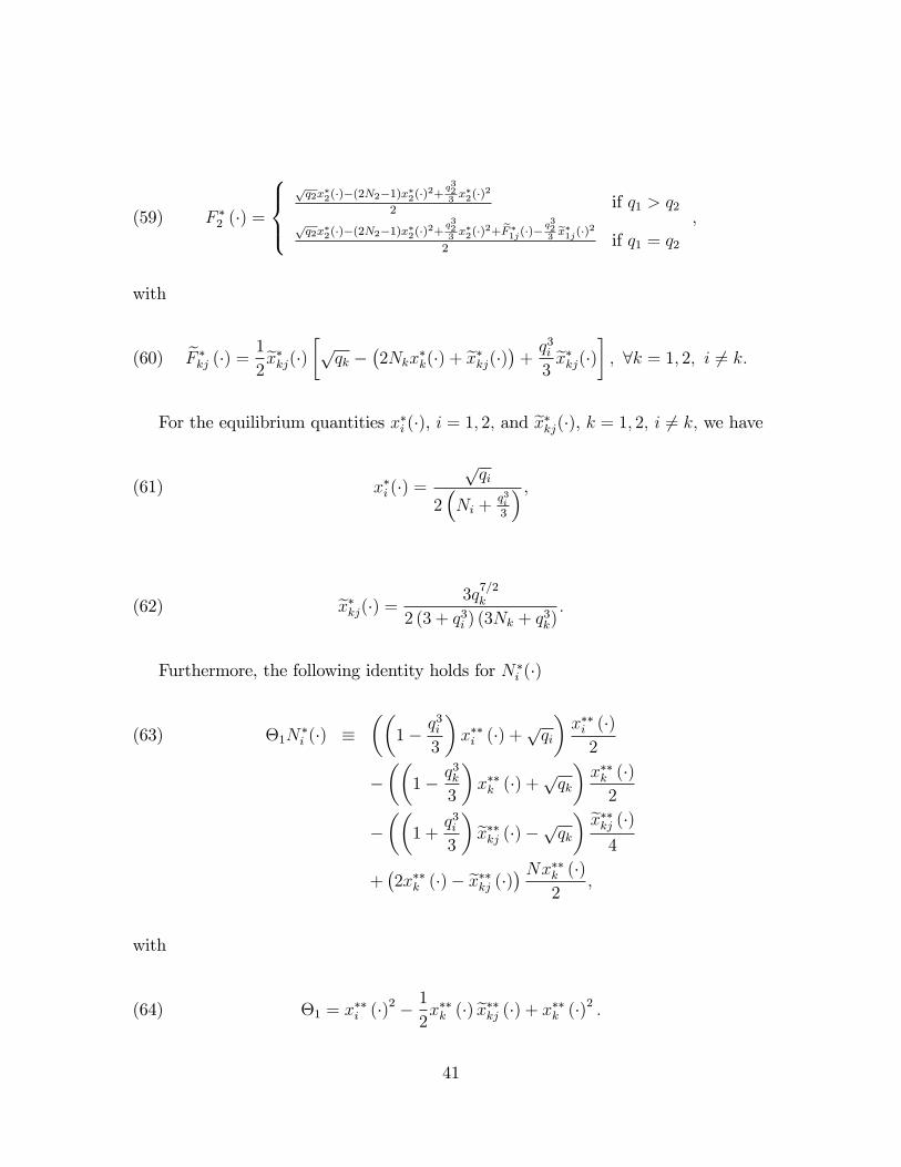
(59) F �2 (�) =
8><>:pq2x�2(�)�(2N2�1)x�2(�)2+
q323x�2(�)2
2if q1 > q2
pq2x�2(�)�(2N2�1)x�2(�)2+
q323x�2(�)2+ eF �1j(�)� q32
3ex�1j(�)2
2if q1 = q2
;
with
(60) eF �kj (�) = 1
2ex�kj(�) �pqk � �2Nkx�k(�) + ex�kj(�)�+ q3i3 ex�kj(�)
�; 8k = 1; 2; i 6= k:
For the equilibrium quantities x�i (�), i = 1; 2; and ex�kj(�), k = 1; 2; i 6= k; we have(61) x�i (�) =
pqi
2�Ni +
q3i3
� ;
(62) ex�kj(�) = 3q7=2k
2 (3 + q3i ) (3Nk + q3k):
Furthermore, the following identity holds for N�i (�)
�1N�i (�) �
��1� q
3i
3
�x��i (�) +
pqi
�x��i (�)2
(63)
���1� q
3k
3
�x��k (�) +
pqk
�x��k (�)2
���1 +
q3i3
� ex��kj (�)�pqk� ex��kj (�)4+�2x��k (�)� ex��kj (�)� Nx��k (�)2
;
with
(64) �1 = x��i (�)
2 � 12x��k (�) ex��kj (�) + x��k (�)2 :41

Numerical Results under Imperfect Competition. Based on the functions
Pi(qi) = max�pqi �Xi � �Xk; 0
; C(xij; qi) = q3i x
2ij=3 and K(Xi) = X2
i ; 8i; k =
1; 2; i 6= k, the equilibrium �xed fees F �1 (�) and F �2 (�) for q1 � q2 are given by
(65) F �1 (�) =�R(X�
1 (�) ; �)� (2N1 � 1)x�1 (�)2 +
q313x�1 (�)
2 + eF �2j � q313ex�2j (�)2
2;
(66) F �2 (�) =
8><>:�R(X�
2(�);�)�(2N2�1)x�2(�)2+
q323x�2(�)
2
2if q1 > q2
�R(X�2(�);�)�(2N2�1)x�2(�)
2+q323x�2(�)
2+eF �1j� q323ex�1j(�)2
2if q1 = q2
;
with
�R(X�1 (�) ; �) = x�1 (�) (
pq1 �N2�x�2 (�) + (1� 2N1)x�1 (�))(67)
+x�1 (�) (N1 � 1)�ex�2j (�) ;
(68) �R(X�2 (�) ; �) =
8>>>><>>>>:x�2 (�)
�pq2 �N1�x�1 (�) + (1� 2N2)x�2 (�)
�if q1 > q2
x�2 (�)�pq2 �N1�x�1 (�) + (1� 2N2)x�2 (�)
�+x�2 (�) (N2 � 1)�ex�1j (�) if q1 = q2
and
(69) eF �kj (�) = 1
2ex�kj (�) �pqk � 4Nkx�k (�) + (1�Ni)�x�i (�) + �q3i3 � 2
� ex�kj (�)� ;8k = 1; 2; i 6= k:
42

For the equilibrium quantities x�i (�), i = 1; 2; and ex�kj (�), k = 1; 2; i 6= k; we have(70) x�i (�) =
2q3k3
pqi +Nk
�4pqi � �
pqk�
4�q3i3+ 2Ni
��q3k3+ 2Nk
��NiNk�2
;
(71) ex�kj (�) = 4q3k3
�q3i3+ 2Ni
�pqk + 2
�q3k3� q3k
3Ni + 2Nk
��pqi �Nk
pqk�
2
2�2 +
q3i3
� h4�q3i3+ 2Ni
��q3k3+ 2Nk
��NiNk�2
i :
Furthermore, the following identity holds for N�i (�)
�2N�i (�) � �2x��i (�)
�pqi +
�2� q
3i
3
�x��i (�)
�(72)
+2x��k (�)�pqk +
�2� q
3k
3� 4N
�x��k (�)
�+2N�x��i (�)x��k (�) +
�2 +
q3i3
� ex��kj (�)2+(�x��i (�) + 4Nx��k (�)�
pqk) ex��kj (�) ;
with
�2 = �8�x��i (�)
2 + x��k (�)2�(73)
+(4x��k (�) + �x��i (�)) ex��kj (�)+4�x��i (�)x��k (�) :
Appendix C
Due to our assumption of perfect competition, the retailers�quality choice has no
impact on the overall quantity in the market. Accordingly, private quality standards
43

only a¤ect the industry pro�t, i.e. I(�) =2Pi=1
[P (qi)X��i �K (X��
i )�N�i C(x
��i ; qi)].
The industry-optimal quality requirement is then given by qI := argmax I(�); result-
ing in qI1 = qI2 = qI : Accordingly, the suppliers split equally between the retailers.
Numerical analysis shows that the industry-optimal quality level qI is increasing in
the total number of suppliers. This is made possible by the decrease in the quantity-
related production costs due to the rise in N: Once the number of suppliers reaches
the threshold value eN; the high-quality retailer D1 imposes a quality standard q�1 that
exceeds the industry-optimal quality level qI . Thus, for all N � eN; a binding MQSleads to a higher industry pro�t. However, a trade-o¤ emerges for N > eN: While ahigher q�2 due to the enforcement of a public MQS approaches the industry-optimal
quality level, the quality requirements q�1 of the high-quality retailer are more likely
to exceed qI . Denoting the best-response function of the high-quality retailer by
r1(q2); the industry-optimal level of the public MQS, qI2, is obtained by maximizing
the industry pro�t with respect to q2, i.e.
(74) qI2 := argmaxq2
I(N�1 (r1(q2); q2) ; r1(q2); q2):
Comparing numerically�I1 = I(qI ; qI)�I(q�1; q�2) and�I2 = I(qI ; qI)�I(r1�qI2�; qI2);
we �nd that �I1 > �I2 always holds. That is, the enforcement of a binding public
MQS increases the industry pro�t also for N > eN:
44

Figures
1.6 1.7 1.8 1.9 2.0 2.1
0.230
0.235
0.240
1.6 1.7 1.8 1.9 2.0 2.1
0.230
0.235
0.240
0.245
0.250
q1
q2
q1D
q2D
ED1DDÝ6Þ
ED2DDÝ6Þ
1.6 1.7 1.8 1.9 2.0 2.1
0.230
0.235
0.240
1.6 1.7 1.8 1.9 2.0 2.1
0.230
0.235
0.240
0.245
0.250
q1
q2
q1D
q2D
ED1DDÝ6Þ
ED2DDÝ6Þ
Figure 1. Pro�t functions and equilibria for N = 10
45

20 30 40 50 60 70
2.0
2.5
3.0
3.5
q2D
q1D
N20 30 40 50 60 70
2.0
2.5
3.0
3.5
q2D
q1D
N
Figure 2. Quality requirements q�1 and q�2 in N
0.2 0.4 0.6 0.8 1.0
2.0
2.2
2.4
2.6
2.8
a
q1D
q2D
0.2 0.4 0.6 0.8 1.0
2.0
2.2
2.4
2.6
2.8
a
q1D
q2D
Figure 3. Quality requirements q�1and q�
2in � for
N = 10
46