NBER WORKING PAPER SERIES

THE STOCK OF EXTERNAL SOVEREIGN DEBT:CAN WE TAKE THE DATA AT ‘FACE VALUE’?

Daniel A. DiasChristine J. Richmond

Mark L.J. Wright

Working Paper 17551http://www.nber.org/papers/w17551

NATIONAL BUREAU OF ECONOMIC RESEARCH1050 Massachusetts Avenue

Cambridge, MA 02138October 2011

The views expressed in this paper are those of the authors and do not necessarily represent those ofthe Federal Reserve Bank of Chicago, the Federal Reserve System, the National Bureau of EconomicResearch, the IMF or IMF policy. The authors thank Marcio Garcia for help researching Braziliandebt issuance, and Moritz Schularick and numerous seminar participants for comments. Further commentswelcome. We are especially grateful to Aart Kraay, Ibrahim Levent and Gloria Moreno of the WorldBank for helping us access these data, and understand its idiosyncrasies. The authors would like tothank the Center for International Business and Economic Research (CIBER) at UCLA for researchsupport. Wright would also like to thank the National Science Foundation for research support undergrant SES-1059829. All remaining errors are our own.

NBER working papers are circulated for discussion and comment purposes. They have not been peer-reviewed or been subject to the review by the NBER Board of Directors that accompanies officialNBER publications.

© 2011 by Daniel A. Dias, Christine J. Richmond, and Mark L.J. Wright. All rights reserved. Shortsections of text, not to exceed two paragraphs, may be quoted without explicit permission providedthat full credit, including © notice, is given to the source.

The Stock of External Sovereign Debt: Can We Take the Data At ‘Face Value’?Daniel A. Dias, Christine J. Richmond, and Mark L.J. WrightNBER Working Paper No. 17551October 2011JEL No. E01,F30,F34,H63

ABSTRACT

The stock of sovereign debt is typically measured at face value. This is a misleading indicator whendebts are issued with different contractual forms. In this paper we construct a new measure of the stockof external sovereign debt for 100 developing countries from 1979 to 2006 that is invariant to contractualform, and illustrate five problems with debt stocks measured at face value. First, we show that correctingfor differences in the contractual form of debt paints a very different quantitative, and in some casesalso qualitative, picture of the stock of developing country external sovereign debt. Second, rankingsof indebtedness across countries, which were historically used to define eligibility for debt forgiveness,are sometimes inverted once we correct for differences in contractual form. Third, the empirical performanceof the benchmark quantitative model of sovereign debt deteriorates by between 40 to 70 percent oncemodel-consistent measures of debt are used. Fourth, we show how the spread of aggregation clausesin debt contracts which award creditors voting power in proportion to the contractual face value mayintroduce inefficiencies into the process of restructuring sovereign debts. Fifth, we show how the useof contractual face values gives issuing countries the ability to manipulate their debt stock data, andillustrate the use of these techniques in practice.

Daniel A. DiasUniversity of Illinois at Urbana Champaign and CEMAPRE109 David Kinley Hall1407 W. Gregory Dr. - MC707Urbana, IL, 61801ddias@illinois.edu

Christine J. RichmondInternational Monetary Fund700 19th Street NWWashington, DC 20431CRichmond@imf.org

Mark L.J. WrightFederal Reserve Bank of Chicago230 South LaSalle St.Chicago, IL 60604and University of California, Los Angelesand also NBERmlwright@econ.ucla.edu

1 Introduction

With few exceptions, data on the stock of sovereign debt are presented at face value.

Defined as the undiscounted sum of future principal repayments, face values can be a mis-

leading indicator of sovereign indebtedness because two debt contracts that possess identical

future cash flows, but divide those cashflows into principal and interest in different ways, will

have different face values.

The emphasis on face values by statisticians and market participants creates at least

five important practical problems. First, the comparison of debt stocks at face value over

time and across countries is misleading in the light of significant differences in the contractual

structure of debt portfolios across countries and over time. For example, low income countries

often borrow from official sources at low interest rates while middle income countries borrow

at market interest rates, while international debt markets have shifted away from bank loans

issued at par towards bonds which are often issued at a discount. Second, as a consequence,

analyses of debt sustainability based on face values will be misleading, with some relatively

highly indebted countries being ineligible for debt relief. Third, it inhibits the assessment

of the empirical relevance of quantitative macroeconomic literature sovereign debt which

typically assumes that all sovereign debt takes the form of zero-coupon bonds. Fourth, it

may introduce inefficiencies into the process of restructuring sovereign debts where creditor

voting power is allocated on the basis of face values. Fifth, the emphasis on face values gives

the issuing country the ability, and sometimes an incentive, to manipulate their debt stock

data. For example, countries can understate the value of their debt stocks by issuing par

bonds (with a high interest rate and low principal) instead of the equivalent discount bonds

(with a lower interest rate and higher principal).

In this paper, we construct a new database of external sovereign debt stocks that

sheds light on the extent of these problems. Motivated by the extensive focus on zero-coupon

bonds in the theoretical literature on sovereign debt, we propose a new measure — the zero-

coupon-equivalent face value — of a country’s external sovereign debt, that is invariant to the

division of the cash flows of a debt contract into principal and interest. We then construct

estimates of our measure of developing country indebtedness using unpublished data on the

cash flows associated with a countries portfolio of external sovereign debts from the World

Bank’s Debtor Reporting System for a sample of 100 developing countries for the period 1979

to 2006.

Our findings bring both good news and bad news for users of data on the stock of

external sovereign debts. The good news is that much of our qualitative understanding of the

market for external sovereign debt is preserved when examined in the light of these new data.

The bad news is that much of our quantitative understanding of international debt markets

needs to be revised. Most dramatically, our new measures of the stock of external sovereign

debt reveal that the upper-middle income countries, and the countries of Latin America and

the Caribbean in particular, are relatively more indebted than other developing countries. In

some cases, the revised measure leads to dramatic changes in the measured relative level of

indebtedness, as in the case of Mexico where the debt stock measure more than doubles in

some years.

Some of our worst news is reserved for the quantitative theoretical literature on sov-

ereign debt and default. It is by now well-known that the benchmark Eaton and Gersovitz

(1981) model of sovereign debt and default, as explored quantitatively by Arellano (2008),

Aguiar and Gopinath (2006) and many others, produces levels of the face value of external

sovereign debt that are between five and ten times smaller than the levels reported in tradi-

tional sovereign debt statistics. This empirical failure is all the more striking when it is noted

that these theoretical models restrict attention to zero-coupon bonds in which all future debt

service payments are regarded as principal, thus producing a maximal value for the model

generated face value of sovereign debt. We show that when data on the stock of external

sovereign debt is constructed using our theoretically consistent zero-coupon equivalent face

value measure, it is almost one-and-one-half times as large as traditional estimates, implying

that the benchmark model produces levels of the stock of sovereign debt between 7.5 and 15

times smaller than those observed in practice.

We also point to a potential problem associated with the more widespread adoption of

aggregation clauses in sovereign debt instruments, as envisaged by the Eurogroup (2010). As

voting rights in the event of a sovereign debt restructuring are proportional to the contrac-

tual face value of a bond, creditors whose debts include a high interest rate will have fewer

voting rights than creditors holding instruments with identical cashflows but lower interest

2

rates. We show using our data that this would have the largest impact on private sector cred-

itors, indicating that more widespread use of aggregation clauses would lead to the relative

subordination of private sector claims. This may explain the reluctance of bondholders to

participate in bond issues including aggregation clauses and, in the event that such clauses

become widespread, may give private sector creditors an incentive to adopt contractual forms

— like zero-coupon bonds — that would maximize their voting power in the event of a future

sovereign debt restructuring. Finally, we also use our data to document at least one prima

facie case of a country varying the contractual form of its debt issuance in order to presents

its external debt position in a more favorable light.

It is important to stress a number of limitations of our analysis. We have nothing to say

about other limitations associated with the use of face values as a measure of indebtedness.

This includes, but is not limited to, concerns about the fact that face values are undiscounted

sums of future cash flows and thus treat debts with different maturity structures as equivalent.

This is closely related to concerns that face values are not accurate measures of the value of

a debt to investors, nor of the cost of servicing the debt to the sovereign country itself. All

of these issues may be summarized as concerns about the rate in which the cash flows of a

debt occurring at different dates should be discounted in forming a measure of indebtedness.

Any attempt to construct discounted values of debt stocks must confront the fact that the

absence of liquid markets for all but a small number of sovereign debts means it is not possible

to extract discount rates from market data. Moreover, it is not always appropriate to use

market discount rates in constructing measures of the cost of servicing a debt to the issuing

country. We discuss these issues, as well as alternative approaches for estimating appropriate

discount rates, in a companion paper (Dias, Richmond, and Wright 2011).

Data limitations mean that we focus entirely on external sovereign debts, despite the

recent surge in interest in the domestic debts of developing countries (for example, Reinhart

and Rogoff 2008). Nonetheless, it is important to stress that the exact same measurement

problem applies to existing estimates of the stock of domestic sovereign debt. Our study of the

contractual structure of developing country sovereign debt and the way it leads to misleading

estimates of indebtedness complements Hall and Sargent’s (1997) analysis of the mismea-

surement of interest payments by the US Treasury. Our focus on contractual structure of

3

sovereign debt per se leads us to focus on a different set of summary measures of indebtedness

than does Hall and Sargent’s emphasis on the US government’s cost of borrowing.

The rest of this paper is organized as follows. Section 2 presents a simple frame-

work that is useful in accounting for sovereign debts and illustrates, using a series of simple

examples, the measurement problems associated with using contractual face values when ag-

gregating debts with different contractual structures. Section 3 describes our data sources.

Section 4 presents our quantitative and qualitative findings for the stock of developing coun-

try external sovereign debt and show by example how changing levels of relative indebtedness

could have affected past eligibility for debt relief. Section 5 focuses on the policy implications

of these data, emphasizing the incentive of countries to manipulate their debt stock data, and

the incentives for creditors to vary the contractual form of their sovereign debts in anticipa-

tion of the more widespread use of aggregation clauses in sovereign debt instruments. Section

6 contains some concluding remarks, while a series of appendices describe our methods, data

sources, and findings in a greater level of detail than that presented in the paper.

2 Conceptual Framework

In this section, we introduce some notation that is helpful for talking about country

debt portfolios. We also define some measures that we will construct later in the paper and

present a series of simple examples to illustrate different debt stock measures, their varying

strengths and weaknesses, and their potential quantitative importance.

2.A Notation

Consider a country that has a portfolio of debt contracts. Each debt contract specifies

a stream of cash flows denominated in different currencies falling due at future dates. We

denote by () the cash flow associated with contract = 1 of country = 1

due at time = 0 1 ∞ denominated in currency = 1 We allow for cashflows to be

defined at =∞ to capture the case of perpetuities for which the principal is never repaid.

Although not a perfect description of the set of all outstanding sovereign debt contracts1, we

restrict attention to contracts that pay, as long as there is no default, a non-state contingent

1On state contingent sovereign debt, see, for example (Grossman and Huyck 1988, Kletzer 2005, and

Alfaro and Kanczuk 2005).

4

claim in a pre-specified set of currencies at a series of pre-specified dates.

The cash flows associated with a debt contract are typically divided into principal

repayments, or amortization () and interest payments (or coupons)

(). We will say

that two debt contracts 0 are equivalent if they specify the same cashflows () = 0

0 ()

for all time periods and currencies for any countries and 0 even if they divide these

cashflows into amortization and interest in different ways; two equivalent debt contracts that

divide cashflows in different ways will be described as having different contractual forms.

Most countries owe debts denominated in a variety of different currencies. In addi-

tion, some debt contracts are issued in multiple tranches, some of which are denominated in

different currencies. If () is the number of units of the numeraire currency, the US dollar,

that can be purchased with one unit of currency then the dollar cashflows of contract

are denoted by dropping the currency subscript or

() =

X

() ()

Likewise, the cashflows of country 0 entire portfolio of debts are denoted by dropping the

contract subscript or

() =X

() () =

X

()

These dollar cashflows are divided into dollar amortization and coupon payments analogously.

2.B Measuring Indebtedness

Almost all of the available data on the stock of outstanding sovereign debt, both domes-

tic and external, is presented at face value.2 The face value, in US Dollars, of debt contract

2The face value of a debt is also sometimes referred to as the nominal value of a debt. For example, the

European statistical agency Eurostat states that “the nominal value is considered equivalent to the face value

of liabilities” (Eurostat 2010 p.305). To avoid confusion with measures of the debt stock that are, or are not,

adjusted for inflation, we do not use the term “nominal value” below.

5

at time is defined to be the undiscounted sum of any future amortization payments, or

() =

∞X=+1

() +

(∞)

In what follows, to distinguish this concept from the measures we introduce below, we will

refer to this as the contractual face value of a debt contract, denoted to capture the

notion that it is calculated using the assignment of cashflows to principal as written in the

original debt contract.

As is well known, there are a number of reasons why contractual face values can be a

misleading measure of total indebtedness. Perhaps the most obvious is that two equivalent

debt contracts can have different contractual face values if they label these cashflows as

amortization and interest in different ways.

Example 1 (Discount vs Par Bonds). Consider two one-period debt contracts both denom-

inated in the same currency issued at time zero and coming due at time one. The first is a

par bond (issued at its contractual face value) with a positive coupon, while the second is a

zero-coupon bond issued at a discount. In the notation introduced above, suppressing currency

subscripts and country superscripts, the stream of payments associated with first debt can be

represented as 1 (1) 0 and 1 (1) 0 while the second has 2 (1) 0 and 2 (1) = 0

We assume that the two bonds are equivalent or that 1 (1) + 1 (1) = 2 (1) and so they

are valued identically by both the country itself and investors. Despite being equivalent, the

par bond has a contractual face value of (0) = 1 (1) which is less than the contractual

face value of the zero coupon bond (0) = 2 (1).

This potential problem with the use of contractual face values to measure relative

indebtedness across countries and over time would be of little concern if the structure of debt

contracts (and hence the split of cashflows into amortization and interest) was roughly con-

stant across countries and over time. This is far from the case in practice. As one example,

low income countries have access to loans at concessional interest rates from creditor country

governments and international institutions that result in a greater share of cashflows being

6

recorded as amortization compared to interest payments than in middle income countries.3

As a result, the relative indebtedness of low income countries may be overstated. As an-

other example, there has been a dramatic shift amongst middle income countries over the

past quarter century away from bank loans, typically issued at par with a positive coupon,

towards bonds which are often issued at a discount. The use of contractual face values is

also problematic when interest rates vary over time. As interest rates rise, the cash flows

associated with a par-bond of a given contractual face value will rise relative to those for

a discount bond with the same contractual face value. Hence, the relative importance of

various lending instruments will vary mechanically with changing interest rates.

To measure indebtedness in a way that is invariant to contractual form, it is necessary

to treat all cash flows as though they are divided into amortization and coupon in the same

proportions. Although this can be done in an infinite number of ways, we focus on a measure

that treats all cashflows as principal, or in other words treats all debt contracts as though

they are zero coupon bonds.4 Specifically, we define the zero-coupon equivalent face value of

a bond contract denoted as

() =

∞X=+1

¡ () +

()¢=

∞X=+1

()

Note that we do not include cash flows that are never paid (paid at infinity) in this definition.5

The difference between the contractual face value of a debt and its zero-coupon equiv-

3The problematic treatment of concessional lending was behind the World Bank’s move to focus on net

present values of debt service in defining eligibility for debt relief (see Claessens et al., 1996 and Easterly,

2001).4Another alternative would be to treat all bonds as though they are par bonds. In 1997, the European

statistical agency introduced new accounting rules for imputing interest payments on a subset of all sovereign

bonds outstanding that amounts to measuring the principal of some discount bonds as though they were

par bonds (Eurostat 1997a,b). Under the new procedures, for both deep-discounted bonds (defined as bonds

whose contractual coupon is less than 50% of the corresponding yield to maturity) and zero coupon bonds, the

difference between the issue price and the face value is treated as an interest payment due at redemption. Note

that discount bonds that do not meet the deep-discount criterion are not treated equivalently. The absence

of data on issue prices, and our aim of constructing a measure that allows for cross-country comparisons of

contractual structure, motivates our preference for the ZCE face value measure.5Undiscounted measures of debt stocks like the ZCE face value return an infinite value for simple per-

petuities such as United Kingdom consols. We do not view this as a weakness of our measure, as simple

perpetuities are typically grouped with common stock for many purposes (for example, the Bank for Inter-

national Settlements treats bank issued perpetuities as Tier 1 capital). In practice, the only sovereign issued

perpetuities of which we are aware are consols, and the United Kingdom is not a member of our dataset.

7

alent (ZCE) value can be very large as the following theoretical examples drawn from the

quantitative literature on sovereign debt demonstrate.

Example 2 (Hatchondo-Martinez/Arellano-Ramanarayanan). In order to keep track of a

portfolio of bonds longer than one period maturity in a computationally tractable way, Hatch-

ondo and Martinez (2009) and Arellano and Ramanarayanan (2009) examine debt contracts

that take the form of a perpetuity with a coupon that decays exponentially at rate Such debt

contracts are ‘memory-less’ so that debt issued at different dates can be linearly aggregated.

With these contracts, a debt with contractual face value of one issued at time pays a one unit

coupon at time +1 or (+ 1) = 1 and a (1− )−+1

coupon, or () = (1− )−+1

at

all dates + 1 In our notation, the contractual face value of a portfolio of such bonds

is given by − = (∞) = while its ZCE face value is given by

− =

¡1 + (1− ) + (1− )

2+

¢=

Hence, the ratio of ZCE to contractual face values is given by 1 which is roughly a 20 fold

difference for ≈ 005 as commonly used in the quantitative sovereign debt literature.

Example 3 (Chatterjee-Eyigungor). Motivated by similar tractability concerns, Chatterjee

and Eyigungor (2009) examine a class of perpetuities that pay a constant coupon () = for

all and mature at rate each period. A portfolio of such bonds issued at time is asso-

ciated with coupon payments of (1− )−

and amortization payments of (1− )−(+1)

in all periods The contractual face value of a portfolio of such bonds is given by

=

¡+ (1− ) + (1− )

2+

¢=

while the ZCE face value is given by

= +

¡(1− ) + (1− )

2+

¢=

(+ (1− ))

For the values used by Chatterjee and Eyigungor (2009) = 003 and = 005 the ratio of

ZCE to contractual face values for these bonds is 157

8

ZCE face values are particularly convenient for comparing levels of indebtedness in the

data with levels produced by models from the recent quantitative literature on sovereign debt

cited above that focus exclusively on zero coupon bonds. They are also useful in calculating

the market price of defaultable debts when recovery rates are positive (see Benjamin and

Wright, 2009). Finally, they are very simple to calculate.

However, this measure also disguises a number of important features of a country’s

stock of sovereign debt, the most notable of which is that it disguises differences in the profile

of payments over time. As discussed in our companion paper Dias, Richmond, and Wright

(2011), there are a number of practical problems associated with the construction of an

appropriate measure of discounted cashflows. These include, but are not limited to, the fact

that: the appropriate discount rate will vary according to the purpose for which the data will

be used; appropriate discount factors will vary over time, across countries and possibly also

over contracts; and, the absence of market prices for all but a small subset of sovereign debts.

These difficulties are reflected in the fact that most studies of discounted debt service flows

use an arbitrary rate that is constant over time and across countries (for example, Easterly

2001 uses the average LIBOR rate while Dikhanov 1986 uses a fixed 10 percent rate).

3 Data Sources

The primary source for statistics on external sovereign debt are derived from the

World Bank’s Debtor Reporting System (DRS) and are compiled in its Global Development

Finance (GDF) publication.6 The DRS has been in existence since 1951 and records detailed

information at the level of an individual loan for external borrowing. All countries that

receive a World Bank loan consent in the loan or credit agreement to provide information

on their external debt. The details of the reporting procedures are described in World Bank

(2000).

One of the purposes of the DRS database is to generate projections of future debt

service obligations of a country under various assumptions. Towards this end, the DRS

6Statistics on external debt are also available from the Joint External Debt Hub (JEDH), which is jointly

maintained by the Bank for International Settlements (BIS), the International Monetary Fund (IMF), the

Organization for Economic Cooperation and Development (OECD), and the World Bank (WB), and combines

data from the DRS with data from creditor and market sources.

9

records the years-to-maturity, interest rate, currency of denomination, and grace period of

each debt contract at each point in time. Such detailed data are only collected for long

term debts (debts with a maturity at issue in excess of one year), therefore all the results

below correspond to long term debt. Based on these data, and combined with forecasts for

the paths of future interest rates (for floating rate debt) and exchange rates, it can be used

to generate projections of debt service denominated in US dollars. We restrict attention to

sovereign debts that are either owed by the public sector of the country, or are owed by

private sector borrowers but are guaranteed by the public sector of the country (public and

publicly guaranteed).

Data on individual loans is confidential and direct access to the DRS is restricted.

The data reported below is derived from an unpublished dataset constructed by World Bank

staff at our request. The World Bank ensured the confidentiality of the loan level data by

aggregating data across multiple loans. To preserve comparability with existing publicly

available World Bank external debt statistics, we use the same interest rate and exchange

rate assumptions that were used in compiling the GDF.

Our data on cashflows begin in 1980 and end in 2007, and for each year we generate

projected cashflows over a forty year time horinzon. To preserve comparability with GDF

data, we denote the sum of cashflows from year onwards as the stock of debt as of the end

of year − 1

4 Results

In this section, we examine the evolution of debt and debt payment terms using our

zero coupon equivalent face value measure, and compare it to results using the standard

contractual face value measure. We begin by examining the behavior of indebtedness at

an aggregate level for all countries, emphasizing the way in which this new measure alters

our understanding of the empirical performance of the benchmark model of sovereign debt

and default. We also discuss the effect of using the new measure on the relative level of

indebtedness across countries and its implications for analyses of debt sustainability, and

examine how the new measure changes our understanding of the composition and evolution

of international debt flows.

10

1.4

1.5

1.6

1.7

0%

10%

20%

30%

40%

50%

60%

1979 1982 1985 1988 1991 1994 1997 2000 2003 2006

Zero Coupon Equivalent Face  Value(LHS: % of Gross National Income)

Nominal Face  Value(LHS: % of Gross National Income)

Ratio of Zero Coupon Equivalent to Nominal Face  Value (RHS)

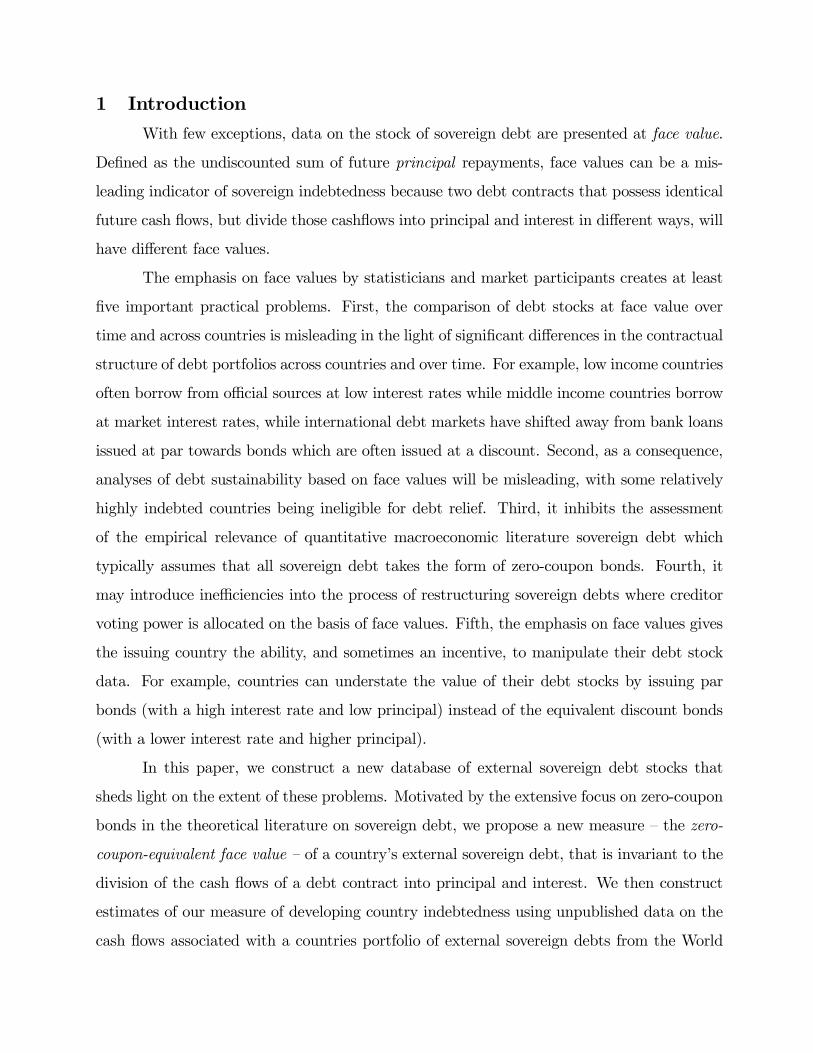
Figure 1: The Face Values of Sovereign Debt

4.A The Level of Indebtedness

Figure 1 plots the ratio of both contractual and ZCE face values of external sovereign

debt as a percent of Gross National Income (GNI), along with the ratio of the two series to

each other. By construction, contractual face values never exceed ZCE face values. Strikingly,

ZCE face values are much larger than contractual face values, always exceeding contractual

face values by at least 40% and sometimes by more than 50%. Whereas the contractual face

value of sovereign debt peaked in 1987 at about 42% of GNI, ZCE face values also peak in

1987 but at 62% of GNI.

Although both series produce a similar picture of the evolution of developing countries

indebtedness over the past 25 years, the relative size of contractual and ZCE face values has

changed substantially. ZCE face values exceeded contractual face values by more than 50

percent during the Latin American debt crisis of the late 1980s, which is the same time that

indebtedness levels reached their peak. The relative difference in levels declined substantially

to just over 40 percent in the early 1990s, reflecting the lower interest rates incorporated into

Brady bonds, before rising back to 45 percent by the turn of the millennium. Even though

overall indebtedness levels declined thereafter, the relative difference between the series did

11

not change much.

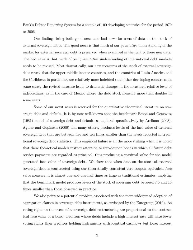
As noted above, the quantitative theoretical literature on sovereign debt has focused

almost exclusively on zero-coupon bonds.7 When assessing the empirical performance of these

models, researchers have compared the level of indebtedness measured using the contractual

face values implied by the zero-coupon bonds that feature in the model, to the contractual face

values of the more complicated portfolio of debts observed in the data. These comparisons

have invariably yielded the conclusion that the benchmark model (with one period debt and

zero recovery rates in the event of a default) produces equilibrium levels of indebtedness

between 5 and 10 percentage points of GNI, which are dramatically below the levels of

indebtedness observed in the data for emerging market countries (as shown in Figure 2,

the ratio of the contractual face value of external sovereign debt to GDP for Latin American

countries have, until very recently, varied between 20% and 50%). This finding has motivated

a large literature to examine modifications of the benchmark model that deliver larger levels

of indebtedness.

The importance of this research agenda is further emphasized once it is understood

that theory and data have not been compared in a theoretically consistent way. If we compare

indebtedness using the theoretically consistent ZCE face values, the empirical performance of

the benchmark model of sovereign debt and default deteriorates further. For the same sample

of Latin American countries, the ratio of the ZCE face value of debt to GDP has tended to

be roughly 50 percent higher than the contractual face value measure, exceeding 80% at the

peak at the turn of the 1990s.

Other issues concerning the comparison of theory to data need to be addressed. Of

great importance is the fact that the models typically focus on one-period (which, given

the common quarterly calibration, amounts to a three-month maturity) debt whereas the

average maturity of debts in the data substantially exceed one year. One approach would be

to define the period length in the theory to be consistent with the average debt maturity in

the data. Another approach would further explore the use of longer maturity debt into these

models as initiated by Hatchondo and Martinez (2009), Arellano and Ramanarayanan (2010)

7See, for example, Arellano (2007), Aguiar and Gopinath (2005), Yue (2010), Tomz and Wright (2007),

and Benjamin and Wright (2009).

12

1.4

1.5

1.6

1.7

1.8

0%

20%

40%

60%

80%

1979 1982 1985 1988 1991 1994 1997 2000 2003 2006

Zero Coupon Equivalent Face  Value(LHS: % of Gross National Income)

Nominal Face  Value(LHS: % of Gross National Income)

Ratio of Zero Coupon Equivalent to Nominal Face  Value (RHS)

Figure 2: The Face Values of Sovereign Debt in Latin American countries.

and Chatterjee and Eyigungor (2009). As shown in the back-of-the-envelope calculations

in the Section 2 examples above, these long maturity debt models produce ZCE face value

indebtedness levels that are between 1.5 and 20 times as large as contractual face values,

bringing their predicted debt levels much closer to the levels measured in this paper.

4.B Relative Indebtedness and Indicators of Debt Sustainability

Moving from contractual to ZCE face values in the computation of debt stocks also

affects the relative ranking of countries by indebtedness. One area in which this is important

is in the application of indicators of debt repayment difficulties. For example, until the mid-

1990s, the World Bank classified countries as “highly indebted” if, amongst other indicators,

the countries external debt (measured at contractual face values) to GDP ratio exceeded

50%. This designation has been used in assessing eligibility for debt relief. When debt stocks

are recomputed using ZCE face values, the measured debt stock increases for all countries

reducing the usefulness of the 50% threshold per se. More importantly, moving to ZCE face

values changes the rank ordering of countries.

Table 1 illustrates this issue by tabulating those countries that were in the neigh-

borhood of the 50% threshold in 1990 (when the threshold was used by the World Bank

13

1990 Debt Face Value/GNI (%)

Contractual ZCE

Countries Designated “Highly Indebted”

Comoros 55.3 66.1

Egypt 56.0 74.8

Papua New Guinea 51.2 68.1

Poland 51.4 69.3

Philippines 54.2 81.1

Togo 53.2 68.6

Countries Designated “Moderately Indebted”

Argentina 37.8 61.0

Cameroon 46.9 62.5

Indonesia 44.0 63.1

Mexico 31.8 67.2

Table 1: Relative Indebtedness Levels in 1990

in awarding the highly indebted designation) and for which the relative ranking is reversed

when examined using ZCE face values. The most dramatic change concerns Mexico where

the contractual face value of debt only just exceeded the 30% threshold of a “moderately

indebted” country in 1990, but whose ZCE face value of 67.2% exceeds the ZCE face values

of four countries designated as highly indebted.8 A similarly large adjustment occurs for

Argentina which, like Mexico, borrows at high market interest rates.

The World Bank has since moved away from the use of contractual face values towards

present discounted values of debt service in designating countries as “highly indebted”. This

was motivated by the issue, discussed above, that contractual face values are misleading

indicators of relative indebtedness when some countries have access to concessional financing

(see Claessens et al., 1996 and Easterly, 2001). However, the absence of widely available

data on the present value of domestic sovereign debt, or on the subcomponents of external

sovereign debt, has meant that researchers have continued to focus on thresholds defined

in terms of contractual face values. For example, Reinhart and Rogoff (2010) study the

relationship between economic growth and indebtedness and find that when external debt

exceeds 60% of GDP, annual growth rates decline by about 2% per year. This finding has

8Besides Comoros, the other three countries that would be considered highly indebted based on the con-

tractual value of the debt in percent of GNI and would have a ZCE debt below Mexico’s are Ghana, Niger

and Uganda.

14

2006 Debt Face Value/GNI (%)

Contractual ZCE

Countries Designated Above Threshold

Dominica 66.9 87.1

Guinea 73.3 85.6

Jamaica 62.2 103.9

Sierra Leone 70.0 79.3

Countries Designated Below Threshold

Panama 48.5 105.4

Uruguay 44.7 90.7

Table 2: Relative Indebtedness Levels in 2006

since become the starting point for a number of other studies of the relationship between

indebtedness and economic growth (see Irons and Bivens, 2010 and Kumar and Woo, 2010).

Table 2 shows how the ordering of countries in the neighborhood of the 60% threshold

varies when indebtedness is measured using ZCE face values for the last year of our data. The

Table identifies two countries whose contractual face values leave them under the threshold,

but whose ZCE face values place them in line with other countries that were previously above

the threshold.

4.C The Evolving Composition of External Sovereign Debt

The extent to which estimates of indebtedness calculated using contractual face values

differ from those calculated using ZCE face values depends on the evolving mix of borrowing

instruments used in international debt markets debt instrument, as well as changes in world

interest rates, and changing circumstances of a country which is reflected in varying country

risk. As a consequence, measurements using ZCE face values paint a quantitatively, and in

some cases also qualitatively, different picture of the evolving composition of the market for

sovereign debt. In this subsection we explore those differences focusing on the changing per-

formance of different debt instruments, different regions, different income groups of countries,

and the currencies in which countries borrow.

Debt Instruments

Figure 3 plots the ratio of ZCE to contractual face values for aggregates of five borrow-

ing instruments. As shown in Figure 3, the ratio of the two face values has declined steadily

15

1.0

1.2

1.4

1.6

1.8

2.0

2.2

2.4

1979 1982 1985 1988 1991 1994 1997 2000 2003 2006

Bonds

Commercial Bank Loans

Official Multilateral Lending

Official Bilateral Lending Other Private 

Lending

Figure 3: Ratio of ZCE to Nominal Face Values by Instrument

over time for both official lending categories as well as the other private category (which

includes, amongst other things, long-term trade credit). Commercial banks loans have also

declined over time, although there were large increases in the late 1980s, and also during

the late 1990s and early 2000s, reflecting the changes in interest rates on commercial bank

loans. The largest changes are due to commercial bond lending, where the ratio jumped from

just over 1.4 in 1986 to over 2.2 in 1990, before stabilizing at roughly 1.8 thereafter. Set

against the example above, this is initially surprising since bonds issued at a discount should,

everything else equal, have higher ZCE to contractual face value ratios than equivalent loan

contracts issued at par. However, this effect is dominated by the fact that the increase in

bond lending was driven by bonds issued by riskier middle income countries facing market

interest rates.

The high average interest rates on private lending to sovereign countries implies that

moving from contractual to ZCE face values increases the relative importance of private sector

lenders in the outstanding stock of sovereign debt. As show in Table 3, while private sector

lending to sovereign countries had fallen to 42.4% by 2000 as measured using contractual

16

Contractual ZCE

1980 1990 2000 1980 1990 2000

Official Lending 43.9 57.9 57.6 39.7 51.2 50.4

(i) Bilateral 30.4 33.9 29.6 26.9 29.4 26.1

(ii) Multilateral 13.5 24.0 28.0 12.8 21.7 24.3

Private Lending 56.1 42.1 42.4 60.3 48.8 49.6

(i) Commercial Banks 36.8 20.6 11.8 42.5 23.6 12.7

(ii) Bonds 4.3 11.1 26.1 4.1 16.3 32.9

(iii) Other 15.0 10.4 4.5 13.8 9.0 4.0

Table 3: Instrument Shares of Total Debt

face values, private sector lending still accounted for 49.6% of lending when measured using

ZCE face values. This was driven almost entirely by the growth in sovereign bond lending,

whose total share of lending increases by 6.8 percentage points in 2000 when moving from

contractual to ZCE face values.

Regions

Moving from contractual to ZCE face values also changes the composition of sovereign

debt across regions. As shown in Figure 4, Latin America and the Caribbean experiences the

largest increase in debt with the ratio of ZCE to contractual face values always above 50%

and even reaching 85% at the beginning of the 1990s. This reflects the greater dependence on

credit provided by private sector lenders at higher interest rates to countries in this region.

The ratio of ZCE to contractual face values is typically low for Sub-Saharan Africa reflecting

their tendency to borrow from official creditors, often at concessional rates.

The differences in the instrument structure of sovereign debt across regions results in

a misstatement of the relative indebtedness of regions. Table 4 presents the share of total

outstanding debt owed by each of the World Bank’s six regional groupings of developing coun-

tries. Adjusting for these measurement issues, Latin America now accounts for an additional

5.2% of total developing country debt, while all other regions are reduced.

Income Levels

Similar patterns appear when we consider income levels. When ZCE and contractual

face values are compared, the difference is smallest for the high and low income countries.

This is because both of these groups of countries are able to borrow at the lowest interest

rates: the high income countries because they are considered a better credit risk, and the low

17

1.0

1.1

1.2

1.3

1.4

1.5

1.6

1.7

1.8

1.9

1979 1982 1985 1988 1991 1994 1997 2000 2003 2006

Latin America and Caribbean

East Asia and Pacific Europe and 

Central AsiaSouth Asia

Sub‐Saharan Africa

Middle East and North Africa

Figure 4: Ratio of ZCE to Nominal Face Values by Region

Contractual ZCE

1980 1990 2000 1980 1990 2000

Latin America & Caribbean 43.4 33.5 36.7 46.5 40.5 41.9

South Asia 10.6 13.5 11.8 8.9 11.4 11.0

East Asia & Pacific 10.5 17.3 22.3 10.3 16.3 20.4

Europe & Central Asia 8.6 10.7 8.7 9.0 10.1 8.4

Middle East & North Africa 14.9 11.7 7.9 14.6 10.3 6.9

Sub-Saharan Africa 12.1 13.3 12.7 10.7 11.4 11.5

Table 4: Regional Shares of Total Debt

18

Contractual ZCE

1980 1990 2000 1980 1990 2000

High Income 2.6 2.6 1.7 2.7 2.3 1.5

Upper Middle Income 53.6 43.5 44.9 56.3 49.9 49.6

Lower Middle Income 36.2 45.4 45.9 34.3 40.8 42.9

Low Income 7.8 8.5 7.4 6.6 7.0 6.0

Table 5: Shares of Total Debt by Income Level

40

50

60

70

80

1979 1982 1985 1988 1991 1994 1997 2000 2003 2006

Introduction of the Euro

All currencies

Number of currencies assuming the 2006 Euro constituents

Figure 5: Number of Currencies Over Time

income countries because they are eligible for concessional loans from official lenders. The

ratio increased for middle income countries with the largest differences, often in excess of

60%, being recorded for the upper middle income countries. As shown in Table 5, moving

from contractual to ZCE face values increases the share of upper middle income countries in

total developing country debt by, on average, roughly 5 percentage points.

Currency

Between 1979 and 2006, the total number of currencies in which outstanding external

sovereign debt is denominated varied between a maximum of 75 (in 1984) and a minimum of

54 (in 2003), as shown in Figure 5. This variation is in part explained by the large reduction

of the number of currencies used in trade credit, and other (non-bank and non-bond) forms

of debt owed to private creditors. These types of loans correspond to the type of instrument

that we labeled as “Other Private Lending” in Figure 6. In Figure 5 we also plot the number

19

10

20

30

40

50

60

1979 1982 1985 1988 1991 1994 1997 2000 2003 2006

Introduction of the Euro

Official Bilateral Lending

Bonds

Commercial Bank Loans

Other Private Lending

Official Multilateral Lending

Figure 6: Number of Currencies by Type of Instrument

of currencies assuming the euro had existed throughout the period.9 The first thing to note

from the comparison of the two lines in Figure 5 is that the difference between the two is

relatively stable as it varies between 10 and 12 currencies.10 The second result to note regards

the fact that after 1999, which corresponds to the official introduction of the Euro, there is

no visible change in the downward trend in the number of currencies used.11 This reflects the

fact that a number of long maturity debt contracts issued originally in the home currency of

a Euro-area member remained outstanding.

Even though the total number of currencies used is relatively large, borrowing is highly

concentrated in a few currencies. To give a better idea of how concentrated borrowing is,

in terms of the currency of choices, in Table 6 we show the 5 most important currencies at

different points in time and also the share in total borrowing that these currencies represent.

9For this purposed we assumed the constituents of the euro in 2006: Austrian Schilling, Belgian Franc,

Netherlands Guilder, Finnish Markkaa, French Francs, German Mark, Irish Pound, Italian Lire, Luxembourg

Franc, Portuguese Escudo, Greek Drachma and Spanish Peseta.10The two currencies that are not present the entire period are the Greek Drachma and the Irish Pound.11The Euro was officially introduced in January 1, 1999, but the cash changeover only took place in January

1, 2002.

20

Contractual Face Values ZCE Face Values

1980 1990 2000 1980 1990 2000

1 USD - 65.4 USD - 57.2 USD - 62.5 USD - 68.9 USD - 62.4 USD - 68.5

2 DM - 7.9 YEN - 12.4 YEN - 13.4 YEN - 7.2 YEN - 11.0 YEN - 11.0

3 YEN - 7.9 DM - 8.7 SDR - 7.7 DM - 7.2 DM - 8.0 SDR - 5.8

4 FF - 5.4 SDR - 5.3 DM - 4.3 FF - 5.2 FF - 4.9 EURO - 4.0

5 GBP - 2.1 FF - 5.3 EURO - 4.2 CHF - 1.8 SDR - 3.9 DM - 3.8

Sum 88.7 88.9 91.9 90.3 90.3 93.1

2006 16.3 17.1 12.3 15.0 15.7 11.2

Table 6: Shares of Total Debt by Currency

In order to see how the importance of the Euro (or its constituents) evolves over time we

also show the relative importance of the debt denominated in the home currencies of Euro-

area members. Table 6 presents various results with respect to the most relevant currencies

in external sovereign debt stocks. First, the U.S. Dollar is the most important currency in

terms of external sovereign debt. Because bonds and commercial banks loans are normally

denominated in U.S. Dollars, and we already know that these instruments tend to have higher

interest rates, it is not surprising that the importance of the US Dollar increases when debt

stocks are measured at ZCE face values. Second, the Japanese Yen and the IMF Special

Drawing Rights (SDR) were the two currencies that gained the most importance during this

period. In particular, in 1980 the SDR did not even make the list of the 5 most important

currencies, but in years 1990 and 2000 it became the fifth and the third most important

currency, respectively, when calculated based on ZCE face values. Similarly, the Yen in 1980

was slightly less important than the Deutsche Mark, but in 1990 and 2000 the share of the

Yen in comparison to the Deutsche Mark was 3 and 4.7 percentage points higher, respectively.

Third, throughout the sample period, and despite some changes in the relative importance of

each currency, 90% of total debt stocks are concentrated in five currencies. Finally, for both

contractual and ZCE face values, the importance of the Euro equivalent declined substantially

between 1990 and 2000, however, from our data it is not possible to tell why the introduction

of the Euro reduced the importance of the currencies that it replaces.

To conclude this part of the paper we show how currency composition varies across

regions and income levels. Table 7 shows the share of debt for different currencies measured

in ZCE face values by region and by income level in the year 2000. In this Table it is shown

21

Euro2006 Yen Pound SDR USD Other

Region

East Asia & Pacific 4.9 25.0 0.6 4.2 64.5 0.7

Europe & Central Asia 22.1 10.3 0.5 4.3 61.3 1.6

Latin America & Caribbean 9.2 5.0 0.5 0.7 83.6 0.9

Middle East & North Africa 24.9 13.0 0.1 1.3 46.4 14.3

South Asia 5.1 12.9 0.4 18.2 62.2 1.1

Sub-Saharan Africa 19.3 5.7 0.7 18.9 45.2 10.2

Income Level

Low 7.1 9.4 1.3 41.8 27.4 12.9

Lower-Middle 10.5 16.4 0.4 6.6 62.8 3.2

Upper-Middle 11.7 6.3 0.5 0.9 79.2 1.4

High 30.6 20.3 1.4 0.2 43.6 3.9

Overall 11.2 11.0 0.5 5.8 68.5 2.9

Table 7: Currency Composition by Region and Income Level

that currency concentration varies both with the region and with the level of income. First,

even though the US Dollar is the most important currency, the level of importance can vary

significantly. For example, in the year 2000, 83.6% of the external debt stock in Latin America

and the Caribbean is denominated in US Dollars, while, for the same year, in Sub-Saharan

Africa only 45.2% of external debt is denominated in US Dollars. Second, there appears

to be some evidence that the external debt stock currency also depends on proximity. In

East Asia and Pacific, the share of debt denominated in Euro and Yen is, respectively, 4.9%

and 25.0%, while in Europe and Central Asia these figures are 22.1% and 10.3%. A similar

explanation may apply to the share of US Dollars in the total debt stock of Latin America and

the Caribbean. In terms of the currency denomination by income level, there are also some

interesting patterns. First, the importance of the US Dollar is only verified for the lower-

and upper-middle income countries. In the case of low income countries the most important

currency is Special Drawing Rights (41.8%) and in the case of high income countries the

difference between the first and the second most important currencies (US Dollar and Euro,

respectively) is much smaller than in the cases of lower- and upper-middle income countries.

22

5 The Policy Implications of Measuring Indebtedness at Contrac-tual Face Value

In this section we point to two areas where the focus on contractual face values gives

market participants an incentive to vary the contractual terms of debt issuance and where

this may affect the outcomes of changes in international economic policy. We begin with a

discussion of the role of face values in determining voting rights in the event of a sovereign debt

restructuring and how this may interact with recent proposals for expanded use of collection

action and aggregation clauses in sovereign debt contracts. We then turn to a discussion of

the ways in which debtors vary their debt issuance when confronted with fiscal rules that are

written in terms of contractual face values or otherwise treat future interest and principal

payments in asymmetric ways.

5.A Face Values and Sovereign Debt Restructuring Negotiations

Another issue for which the distinction between principal and interest can be important

relates to the process by which sovereign debts are restructured. Since 2003, sovereign bonds

issued under NewYork law have included collective action clauses which specify the conditions

under which the terms of the bond may be changed. As one example of such a clause, Brazil’s

10.25% Global BRL Bonds due in 202812 specifies that “the holders of not less than 85% (in

the case of Collective Action Securities designated “Type A” or having no designation as to

“Type”) or 75% (in the case of Collective Action Securities designated “Type B”) in aggregate

principal amount of the outstanding debt securities of that series, voting at a meeting or by

written consent, must consent to any amendment, modification, change or waiver with respect

to”[emphasis added], amongst other things, repayment terms. That is, voting rights in the

event of a restructuring are allocated in proportion to a debt’s contractual face value

If all debts covered by a collective action clause divide repayments into principal and

interest in the same way, then voting in proportion to principal holdings will produce the

same outcomes as voting in proportion to a creditors overall exposure. When debt contracts

divide future cash-flows in different ways either explicitly, or implicitly due to non-stationary

repayment terms and different maturities, this will not be the case. In particular, the holders

12http://www.sec.gov/Archives/edgar/data/205317/000119312510234571/d424b5.htm

23

of debts issued with higher coupons will have less voting rights than holders of equivalent

debts with lower coupons.

This issue is of practical importance today, and is likely to increase in importance over

time as aggregation clauses — clauses that group together different debt securities in the even

of a renegotiation of sovereign debt — become more widespread. Uruguay has already issued

bonds containing aggregation clauses13 while other countries plan to do so in the future.

In Europe, for example, the Eurogroup statement of November 28, 2010 (Eurogroup 2010)

commits its members to introduce, starting in 2013, “aggregation clauses allowing all debt

securities issued by a Member State to be considered together in negotiations” [emphasis

added]. Proposals to introduce similar aggregation clauses in non-Euro-area sovereign bonds

have also been discussed in policy circles (IMF, 2002). Interpreting this policy broadly,

future debt restructuring negotiations would then involve negotiations across a very diverse

set of debt instruments including potentially debts issued by both official and private sector

creditors, banks and bondholders, issued at different maturities and in different currencies

under different governing laws. As a result of this diversity, shares of outstanding principal are

unlikely to be representative of the relative financial exposure of different creditors. Moreover,

it is conceivable that a desire to maximize voting power in the event of a restructuring might

influence the form of debt instrument desired by creditors.

To obtain a sense of the practical significance of this issue, suppose that all debt secu-

rities were modified to contain aggregation clauses and that otherwise the contractual form of

a country’s debts remains the same as their level in 2006. If we restrict attention to sovereign

debt owed to private creditors, one potential source of conflict lies in the competing interests

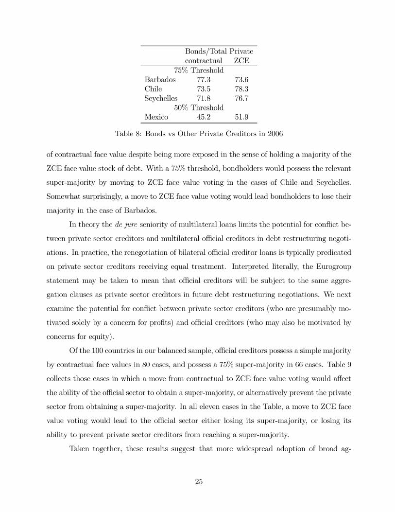
of banks and bondholders. Table 8 collects the countries for which, in 2006, voting in pro-

portion to contractual face value would have yielded different results than in a restructuring

where voting was in proportion to zero-coupon equivalent face value. With a simple majority

voting threshold, the bondholders of Mexico would hold a minority share calculated in terms

13Uruguay’s May 2003 issue of 10.50% Bonds due 2006 contained a clause allowing it to mod-

ify the reserved matters of two or more securities if “the holders of not less than 85% in

aggregate principal amount of the outstanding debt securities of all series that would be af-

fected by that modification (taken in aggregate), and ... 66-2/3% in aggregate principal

amount of the outstanding debt securities of that series (taken individually)” agree. (See

http://www.sec.gov/Archives/edgar/data/102385/000095012303011424/y90432b5e424b5.htm#026).

24

Bonds/Total Private

contractual ZCE

75% Threshold

Barbados 77.3 73.6

Chile 73.5 78.3

Seychelles 71.8 76.7

50% Threshold

Mexico 45.2 51.9

Table 8: Bonds vs Other Private Creditors in 2006

of contractual face value despite being more exposed in the sense of holding a majority of the

ZCE face value stock of debt. With a 75% threshold, bondholders would possess the relevant

super-majority by moving to ZCE face value voting in the cases of Chile and Seychelles.

Somewhat surprisingly, a move to ZCE face value voting would lead bondholders to lose their

majority in the case of Barbados.

In theory the de jure seniority of multilateral loans limits the potential for conflict be-

tween private sector creditors and multilateral official creditors in debt restructuring negoti-

ations. In practice, the renegotiation of bilateral official creditor loans is typically predicated

on private sector creditors receiving equal treatment. Interpreted literally, the Eurogroup

statement may be taken to mean that official creditors will be subject to the same aggre-

gation clauses as private sector creditors in future debt restructuring negotiations. We next

examine the potential for conflict between private sector creditors (who are presumably mo-

tivated solely by a concern for profits) and official creditors (who may also be motivated by

concerns for equity).

Of the 100 countries in our balanced sample, official creditors possess a simple majority

by contractual face values in 80 cases, and possess a 75% super-majority in 66 cases. Table 9

collects those cases in which a move from contractual to ZCE face value voting would affect

the ability of the official sector to obtain a super-majority, or alternatively prevent the private

sector from obtaining a super-majority. In all eleven cases in the Table, a move to ZCE face

value voting would lead to the official sector either losing its super-majority, or losing its

ability to prevent private sector creditors from reaching a super-majority.

Taken together, these results suggest that more widespread adoption of broad ag-

25

Official/Total

contractual ZCE

75% Threshold

Brazil 30.3 21.0

Dominica 76.3 71.3

Malta 31.3 19.2

Turkey 30.7 24.4

Uruguay 31.3 21.2

66% Threshold

Grenada 46.3 27.1

St. Lucia 68.0 65.5

50% Threshold

Ecuador 57.8 43.6

El Salvador 58.3 41.1

Philippines 50.7 40.6

St. Vincent & Gr. 50.8 49.9

Table 9: Official vs Private Creditors in 2006

gregation clauses with voting based on contractual face values would lead to the effective

subordination of private sector claims. This may, in turn, partly explain the reluctance of

private sector creditors to participate in bond issues with aggregation clauses and their favor

with policy makers. However, these calculations also suggest that, should the official sector

succeed in encouraging widespread adoption of broadly defined aggregation clauses, private

sector creditors will have an incentive to adopt contractual forms (such as zero-coupon bonds)

that maximize the contractual face value of their claim and so maximize their voting power

in the event of a restructuring. And in at least eleven cases, this would result in the effective

subordination of official sector claims.

5.B Manipulation of Fiscal Statistics

There is often an incentive for the government of a country to present data on debt

stocks, and fiscal deficits, in a favorable light. Sometimes this incentive is the result of specific

accounting rules, such as the debt stock limits of the USA and Denmark, the budget deficit

and debt stock restrictions imposed by the Maastricht Treaty on EU countries, or fiscal targets

imposed by IMF lending arrangements. In other cases, the incentive arises implicitly from

the desire to improve domestic political performance or the terms on which external debts

26

can be issued. The most common form of manipulation involves using proceeds from the

sale of assets, ranging from privatization to the development of currency swaps, as used by

Greece, to substitute for debt issuance. In addition, when the relevant statistics that are being

targeted treat principal and interest asymmetrically, governments have also manipulated the

contractual forms of new debt issuance to meet specific targets and disguise an underlying

deterioration in the country’s fiscal position (see the discussion in Easterly 1999, Piga 2001,

Milesi-Ferretti 2004, and Koen and van den Noord 2005).

The asymmetric treatment of interest and principal in fiscal targets is common. For

example, the US debt ceiling, which has been the subject of much recent debate, applies

to the contractual face value of US sovereign debt, with the relevant law stating that “The

face amount of obligations issued under this chapter [31 USCS §§ 3101 et seq.] and the

face amount of obligations whose principal and interest are guaranteed by the United States

Government (except guaranteed obligations held by the Secretary of the Treasury) may not

be more than $ 14,294,000,000,000 outstanding at one time” (31 U.S.C. 3101(b)). Likewise,

the Excessive Deficits Procedure of the Maastricht Treaty specifies a debt threshold of 60%

of GDP where “‘debt’ means total gross debt at nominal value outstanding at the end of

the year and consolidated between and within the sectors of general government” (Article

2.d) and where “the nominal value is considered equivalent to the face value of liabilities”

(Eurostat 2010 p.305).

In the early years of the Maastricht Treaty, changes in the relative issuance of low-face-

value-high-coupon and high-face-value-low-coupon debt by EU governments to understate

either debt stocks or fiscal deficits appears to have been common. Koen and van der Noord

(2005) document more than twenty cases in which the treatment of interest payments in the

fiscal accounts by EU countries was questionable. Perhaps the best known example of these

comes from Italy, which reduced the contractual face value of the stock of government debt by

1.9 percentage points of GDP in 2002 when Italy was close to the Maastricht debt threshold.

In this example, the Italian Treasury with the Banca d’Italia bought back long-term bonds

with a low coupon in exchange for a smaller amount of bonds with a much higher coupon.

The use of ZCE face values would eliminate this incentive and, indeed, in response to these

concerns about the manipulation of debt and budget statistics, Eurostat introduced new rules

27

in 1997 requiring the imputation of interest payments on zero coupon debts and other deeply

discounted bonds so that measured principal and interest payments for these classes of debt

contracts would be treated symmetrically with debts issues at par (Eurostat 1997a, b).

Another example of the asymmetric treatment of interest and principal in fiscal targets

comes from IMF Stand-By Arrangements with Argentina throughout the 1990s.14 In the 1991

Stand-By Arrangement, the performance criteria targeted the overall cash balance of the

government (which included interest payments) as well as the stock of outstanding disbursed

external debt (IMF, 2001). By contrast, in the 1996 Stand-By Arrangement, the performance

criteria targeted fiscal expenditures excluding interest payments on debt (IMF, 1996; see also

IMF IEO, 2004). As a consequence, starting in 1996 Argentina had an incentive to switch

to issuing low-face-value high-coupon debt in order to meet the IMF targets for non-interest

expenditures.

Our database shows that Argentina responded to this incentive. Figures 7 and 8 plot

the ratio of the undiscounted sum of future interest payments to the contractual face value

of outstanding debt by instrument for both Deutsche Mark and U.S. Dollars denominated

Argentine external sovereign debt. Both Figures show that, starting in 1996, the ratio of

future interest payments to contractual face values for sovereign bonds jumps dramatically.

Moreover, this pattern is not repeated for any other class of debt instrument, suggesting that

it does not reflect some other change in the environment affecting Argentine borrowing.

6 Conclusion

Data on the stock of sovereign debt is typically presented at contractual face value. De-

fined as the sum of future principal repayments, contractual face values can paint a misleading

picture of indebtedness because they treat debts with identical total cashflows differently if

they have different contractual forms (that is, if the debts divide these cashflows into prin-

cipal and interest in different ways). In this paper, we introduced a measure of the stock of

sovereign debt that is invariant to contractual form — the zero coupon equivalent face value —

14Other cases no doubt exist. Easterly (1999, 2001) states that Brazil issued zero coupon debt in 1998 so

as to understate current interest expenditures. However, we have been unable to uncover any other sources

of information on this episode.

28

0%

20%

40%

60%

80%

100%

1990 1992 1994 1996 1998 2000 2002 2004 2006

Bonds

Commercial Bank Loans

Official BilateralLending

Figure 7: Ratio of the sum of interest to the sum of principal payments by instrument in

Deutsche Marks for Argentina.

0%

40%

80%

120%

160%

200%

1990 1992 1994 1996 1998 2000 2002 2004 2006

Bonds

Commercial Bank Loans

Official BilateralLending

Official MultilateralLending

Figure 8: Ratio of the sum of interest to the sum of principal payments by instrument in U.S.

Dollars for Argentina.

29

and applied it to data on the external sovereign debt of 100 developing countries from 1979

to 2006.

We found that using a measure that is invariant to contractual form paints a very

different quantitative picture, and in some cases also a different qualitative picture, of the

stock of developing country external sovereign debt. For example, according to our measure,

the countries of Latin America and the Caribbean are relatively more indebted than countries

in other regions because of their access to market sources of funding which charge higher

interest rates. The rankings of individual countries in terms of their indebtedness, which

historically was used as a criterion for eligibility for debt relief, can also change significantly.

For example Mexico, which was classified as moderately indebted by the World Bank in 1990

based on the total stock of external sovereign debt at contractual face value, is more heavily

indebted than some countries that were classified as highly indebted, once indebtedness is

measured in a way that is invariant to contractual form.

Our zero-coupon equivalent face value measure is particularly useful for comparing

the data with the growing quantitative theoretical literature on sovereign debt that typically

assumes that all debts take the form of zero-coupon bonds. As is well known, models in this

literature produce zero-coupon face value debt levels that are almost an order of magnitude

smaller that the contractual face value debt stock data available. When our theoretically

consistent zero-coupon equivalent face value measure is used, the empirical performance of

these models is found to be on average between an additional 40 and 80 percent worse than

previously thought.

Finally, we pointed to the incentives for both creditors and debtors to manipulate

the contractual structure of debts in light of the emphasis on contractual face values. For

creditors, voting power during debt restructuring negotiations is in proportion to contractual

face value. As aggregation clauses — which combine different debt instruments for the purpose

of one restructuring — in debt instruments become more widespread, creditors holding high

contractual face value debt will therefore possess a voting advantage. Using our data, we

establish that this has the potential to effectively subordinate private sector bondholders.

Similarly, we show that debtors have an incentive to manipulate their debt statistics when

they are evaluated on measures that emphasize principal repayment (such as contractual face

30

values), or that emphasize interest payments, and use our data to make a prima facie case

for manipulation by one country in our dataset.

The paper points to the desirability for further work in at least three directions. First,

in the light of a surge of recent interest, it would be desirable to construct a similar contract

invariant measure of domestic sovereign debt. Second, as emphasized above, our paper has

nothing to say about the desirability or appropriateness of different methods for discounting

cash flows to arrive at an appropriate valuation for the stock of external sovereign debt. In a

companion paper (Dias, Richmond and Wright 2011) we present a theoretical framework that

suggests that the appropriate discount rate will vary according to the purpose for which the

values will be used, as well as across countries and over time. We also present several methods

for implementing the implications of that theory. Third, and relatedly, our paper also has

little to say about the maturity structure of external sovereign debts, which has been a topic

of recent academic and policy interest. In future work we aim to use our data to construct a

comprehensive set of estimates of the maturity of external sovereign debts, disaggregated by

country, instrument, and currency of issue, which we will then use to discipline the existing

models of the maturity structure of external sovereign debt.

References

[1] Aguiar, M. and G. Gopinath. 2006. “Defaultable debt, interest rates and the current

account.” Journal of International Economics 69: 64-83.

[2] Alfaro, L. and F. Kanczuk. 2005. Sovereign debt as a contingent claim: a quantitative

approach. Journal of International Economics 65(2): 297-314.

[3] Arellano, C. 2008. “Default risk and income fluctuations in emerging markets.”American

Economic Review 98(3): 690-712.

[4] Arellano, C. and A. Ramanarayanan. 2010. Default and the maturity structure in sov-

ereign bonds. University of Minnesota Department of Economics working paper, mimeo.

[5] Chatterjee, S. and B. Eyigungor. 2010. Maturity, indebtedness, and default risk. Federal

Reserve Bank of Philadelphia Working Paper No. 10-12.

31

[6] Dias, D., C. Richmond, and M.L.J. Wright (2011). “Valuing the Stock of external Sov-

ereign Debt.” Working paper, University of California, Los Angeles.

[7] Dikhanov, Y. (2006). "Historical Present Values of Debt in Developing Countries, 1980-

2002." World Bank Working Paper.

[8] Easterly, W., (2001a) Growth implosions, debt explosions, and my Aunt Marilyn: Do

growth slowdowns cause public debt crises? World Bank Policy Research Working Paper

2531.

[9] Easterly, W., When Is Fiscal Adjustment an Illusion? Economic Policy, 1999. 14(28):

p. 55-86.

[10] Eurostat, Deficit and Debt: Eurostat Rules on Accounting Issues. Eurostat Press Release,

1997. 97(10).

[11] Eurostat, Accounting Rules: Complementary Decisions of Eurostat on Deficit and Debt.

Eurostat Press Release, 1997. 97(24).

[12] Eurostat, Manual on Government Deficit and Debt: Implementation of ESA 95. 2010,

Luxembourg: Eurostat.

[13] Grossman, H. I. and J. B. Van Huyck. 1988. Sovereign debt as a contingent claim:

excusable default, repudiation, and reputation. American Economic Review 78(5): 1088-

1097.

[14] Hall, G. J. and T. J. Sargent. 2007. “Accounting Properly for the Government’s Interest

Costs.” Federal Reserve Bank of Chicago Economic Perspectives, vol. 21, no. 4, 18-28.

[15] Hatchondo, J. C. and L. Martinez. 2009. “Long-duration bonds and sovereign defaults.”

Journal of International Economics 79: 117-125.

[16] International Monetary Fund Independent Evaluation Office, Report on the Evaluation

of the Role of the IMF in Argentina, 1991—2001, in Independent Evaluation Office Eval-

uation Report. 2004, International Monetary Fund.

32

[17] International Monetary Fund. 1991. Argentina - Request for Stand-By Arrangement -

Letter of Intent. EBS/91/107, June 28, 1991.

[18] International Monetary Fund. 1996. Argentina - Request for Stand-By Arrangement.

EBS/96/45, March 15, 1996.

[19] Kletzer, K. 2005. Sovereign debt, volatility, and insurance. Federal Reserve Bank of

San Franscisco Working Paper 2006-05.

[20] Koen, V. and P. van den Noord, Fiscal Gimmickry in Europe. OECD Working Paper,

2005(417).

[21] Milesi-Ferretti, G.M., 1997. “Good, bad or ugly? On the effects of fiscal rules with

creative accounting.” Journal of Public Economics, 88(1-2): p. 377-394.

[22] Piga, G., Do Governments Use Financial Derivatives Appropriately? Evidence from

Sovereign Borrowers in Developed Economies. International Finance, 2001. 4(2): p. 189-

219.

[23] Reinhart, C. M. and K. S. Rogoff. 2008. The forgotten history of domestic debt. NBER

Working Paper No. 13946.

[24] Reinhart, C.M. and K.S. Rogoff. 2010. “Growth in a Time of Debt.” American Economic

Review Papers and Proceedings, 00(2): p. 573-578.

[25] World Bank (2000). Debtor Reporting System Manual. World Bank Washington D.C.

[26] World Bank (various). Global Development Finance. World Bank Washington D.C.

[27] Yue, V. Z. 2010. “Sovereign default and debt renegotiation.” Journal of International

Economics 80(2): 176-187.

7 Appendix A: Country List

In our calculations we used a sub-set of the total number of countries that are available

in the dataset. The reason was that we wanted to use a balanced panel in order to avoid

potential attrition problems. In the original dataset there are 138 countries, while in our

33

Country Region Inc.Group Country Region Inc.Group

Algeria MENA UMI El Salvador LAC LMI

Argentina LAC UMI Equatorial Guinea SSA HI

Bangladesh SA LI Ethiopia SSA LI

Barbados LAC HI Fiji EAP UMI

Belize LAC LMI Gabon SSA UMI

Benin SSA LI Gambia, The SSA LI

Bolivia LAC LMI Ghana SSA LI

Botswana SSA UMI Grenada LAC UMI

Brazil LAC UMI Guatemala LAC LMI

Bulgaria ECA UMI Guinea SSA LI

Burkina Faso SSA LI Guinea-Bissau SSA LI

Burundi SSA LI Guyana LAC LMI

Cameroon SSA LMI Haiti LAC LI

Cape Verde SSA LMI Honduras LAC LMI

Central Afr. Republic SSA LI Hungary ECA HI

Chad SSA LI India SA LMI

Chile LAC UMI Indonesia EAP LMI

China EAP LMI Jamaica LAC UMI

Colombia LAC UMI Jordan MENA LMI

Comoros SSA LI Kenya SSA LI

Congo, Dem. Republic SSA LI Lesotho SSA LMI

Congo, Republic SSA LMI Liberia SSA LI

Costa Rica LAC UMI Madagascar SSA LI

Cote D’Ivoire SSA LMI Malawi SSA LI

Djibouti MENA LMI Malaysia EAP UMI

Dominica LAC UMI Maldives SA LMI

Dominican Republic LAC UMI Mali SSA LI

Ecuador LAC LMI Malta ECA HI

Egypt MENA LMI Mauritania SSA LI

work sample we use 100 countries. Table 10 contains this list of countries. In Appendix C

we show that our results are qualitatively identical when we use the full set of countries.

Note: The region and income level identifiers are defined as follows. Region: EAP

= East Asia and Pacific; ECA = Europe and Central Asia; LAC = Latin America and

Caribbean; MENA = Middle East and North Africa; SA = South Asia; SSA = Sub-Saharan

Africa. Income: LI = Low Income; LMI = Lower Middle Income; UMI = Upper Middle

Income; HI = High Income.

34

Country Region Inc.Group Country Region Inc.Group

Mauritius SSA UMI Sierra Leone SSA LI

Mexico LAC UMI Solomon Islands EAP LMI

Morocco MENA LMI Sri Lanka SA LMI

Mozambique SSA LI St. Kittis and Nevis LAC UMI

Nepal SA LI St. Lucia LAC UMI

Nicaragua LAC LMI St. Vicent and Gre. LAC UMI

Niger SSA LI Sudan SSA LMI

Nigeria SSA LMI Swaziland SSA LMI

Oman MENA HI Syria MENA LMI

Pakistan SA LMI Tanzania SSA LI

Panama LAC UMI Thailand EAP LMI

Papua New Guinea EAP LMI Togo SSA LI

Paraguay LAC LMI Tonga EAP LMI

Peru LAC UMI Trinidad and Tobago LAC HI

Philippines EAP LMI Tunisia MENA LMI

Poland ECA UMI Turkey ECA UMI

Rwanda SSA LI Uganda SSA LI

Samoa EAP LMI Uruguay LAC UMI

Sao Tome & Principe SSA LMI Vanuatu EAP LMI

Senegal SSA LI Venezuela LAC UMI

Seychelles SSA UMI Zambia SSA LI

Table 10: List of countries used in the calculations

35

0%

10%

20%

30%

40%

50%

1979 1982 1985 1988 1991 1994 1997 2000 2003 2006

GDF data

Our data

Figure 9: Comparing publicly available data with our data - aggregate values. Units: % GNI.

8 Appendix B: Comparison To World Bank Published Data

As argued above, our data when aggregated, almost replicates the publicly available

data that is published by the World Bank. In this appendix our goal is to provide evidence

supporting this claim.

In Figure 9 we compare some of our data with the data that is publicly available in

the World Bank Global Development Financial indicators dataset. As it is visible in Figure

9 the differences between the two series are very small which shows that, at least at the

aggregate level, our data is very similar to the data that is publicly available. Our data tends

to systematically produce higher values for the debt stocks than those based on publicly

available data, but the correlation between the two series is 99.2%. This comparison is only

done for those countries that we used in our analyses and for which there is publicly available

data.

Because in the paper we focus many of our analyses on the composition of debt in

terms of instrument and also on the geographical distribution of debt stocks we also provide

some comparisons between our data and the data that is publicly available. Tables 11 and 12

36

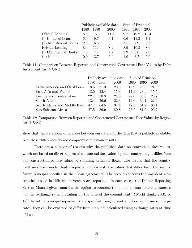
Publicly available data Sum of Principal

1980 1990 2000 1980 1990 2000

Official Lending 88 163 116 97 192 134

(i) Bilateral Loans 60 97 61 66 113 71

(ii) Multilateral Loans 28 66 55 31 79 63

Private Lending 84 114 82 89 103 86

(i) Commercial Banks 75 77 22 79 66 26

(ii) Bonds 09 37 60 10 37 60

Table 11: Comparison Between Reported and Constructed Contractual Face Values by Debt

Instrument (as % GNI)

Publicly available data Sum of Principal

1980 1990 2000 1980 1990 2000

Latin America and Caribbean 185 310 200 199 285 216

East Asia and Pacific 180 224 153 179 239 155

Europe and Central Asia 227 388 243 226 366 257

South Asia 134 266 223 146 301 224

North Africa and Middle East 477 645 374 478 612 381

Sub-Saharan Africa 275 869 808 269 819 902

Table 12: Comparison Between Reported and Constructed Contractual Face Values by Region

(as % GNI)

show that there are some differences between our data and the data that is publicly available,

but, these differences do not compromise our main results.

There are a number of reasons why the published data on contractual face values,

which are based on direct reports of contractual face values by the country, might differ from

our construction of face values by summing principal flows. The first is that the country

itself may have inadvertently reported contractual face values that differ form the sum of

future principal specified in their loan agreements. The second concerns the way debt with

tranches issued in different currencies are reported. In such cases, the Debtor Reporting

System Manual gives countries the option to combine the amounts from different tranches

“at the exchange rates prevailing on the date of the commitment” (World Bank, 2000, p.

12). As future principal repayments are specified using current and forecast future exchange

rates, they can be expected to differ from amounts calculated using exchange rates at time

of issue.

37

Country # Years Country # Years

Afghanistan 28 Lithuania 17

Albania 18 Macedonia 28

Angola 28 Moldova 16

Armenia 16 Mongolia 22

Azerbaijan 14 Montenegro 7

Belarus 15 Myanmar 28

Bhutan 27 Romania 28

Bosnia-Herzegovina 28 Russian Federation 28

Cambodia 28 Serbia 28

Croatia 20 Slovak Republic 28

Eritrea 14 Somalia 28

Estonia 15 South Africa 17

Georgia 15 Tajikistan 15

Iran 28 Turkmenistan 15

Kazakhstan 15 Ukraine 15

Kyrgyz Republic 15 Uzbekistan 15

Laos 28 Vietnam 28

Latvia 16 Yemen 28

Lebanon 28 Zimbabwe 28

Table 13: List of countries in our dataset that were excluded from the analysis.

9 Appendix C: Results From Unbalanced Sample

In the data we obtained from the World Bank there were a total of 138 countries but

we only used a subset of 100 countries in our calculations. The main reason for this difference

is the fact that we wanted to have a balanced sample of countries and avoid noise in our

results that is caused by changes in the composition of the sample. There are two reasons

that motivated the exclusion of 38 countries: 1) for 17 countries, the data we obtained from

the World Bank contains information for the entire sample period (1979-2006), but, we were

not able to find reliable estimates of Gross National Income (GNI) for these countries over

the whole sample period; 2) for the remaining 21 countries, the data on debt did not cover

the entire sample period and for the reasons discussed above we decided to exclude them

from the analysis. This last group of countries is mostly composed of former Soviet Union

countries and other Eastern European countries - there are some exceptions. Below, we list

the countries for which we have data but did not use in our analysis.

The set of countries that were excluded is not random and therefore it is expected

38

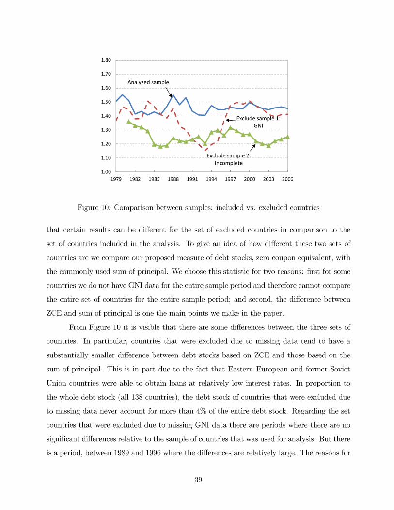
1.00

1.10

1.20

1.30

1.40

1.50

1.60

1.70

1.80

1979 1982 1985 1988 1991 1994 1997 2000 2003 2006

Analyzed sample

Exclude sample 1: GNI

Exclude sample 2: Incomplete

Figure 10: Comparison between samples: included vs. excluded countries

that certain results can be different for the set of excluded countries in comparison to the

set of countries included in the analysis. To give an idea of how different these two sets of

countries are we compare our proposed measure of debt stocks, zero coupon equivalent, with

the commonly used sum of principal. We choose this statistic for two reasons: first for some

countries we do not have GNI data for the entire sample period and therefore cannot compare

the entire set of countries for the entire sample period; and second, the difference between

ZCE and sum of principal is one the main points we make in the paper.

From Figure 10 it is visible that there are some differences between the three sets of

countries. In particular, countries that were excluded due to missing data tend to have a

substantially smaller difference between debt stocks based on ZCE and those based on the

sum of principal. This is in part due to the fact that Eastern European and former Soviet

Union countries were able to obtain loans at relatively low interest rates. In proportion to

the whole debt stock (all 138 countries), the debt stock of countries that were excluded due

to missing data never account for more than 4% of the entire debt stock. Regarding the set

countries that were excluded due to missing GNI data there are periods where there are no

significant differences relative to the sample of countries that was used for analysis. But there

is a period, between 1989 and 1996 where the differences are relatively large. The reasons for

39

these differences are not clear to us. Despite these differences, our main conclusions in the

paper are not affected by the sample that we use and they simply reflect that there is some

heterogeneity with respect to some of the issues we raise.

40