the stochastic bifurcation behaviour of speculative financial markets

Physica A 387 (2008) 3837–3846www.elsevier.com/locate/physa

The stochastic bifurcation behaviour of speculativefinancial marketsI

Carl Chiarellaa,∗, Xue-Zhong Hea, Duo Wangb, Min Zhenga,b

a School of Finance and Economics, University of Technology, Sydney, PO Box 123, Broadway, NSW 2007, Australiab School of Mathematical Sciences, Peking University, Beijing 100871, PR China

Available online 18 January 2008

Abstract

This paper establishes a continuous-time stochastic asset pricing model in a speculative financial market with fundamentalistsand chartists by introducing a noisy fundamental price. By application of stochastic bifurcation theory, the limiting marketequilibrium distribution is examined numerically. It is shown that speculative behaviour of chartists can cause the market priceto display different forms of equilibrium distributions. In particular, when chartists are less active, there is a unique equilibriumdistribution which is stable. However, when the chartists become more active, a new equilibrium distribution will be generatedand become stable. The corresponding stationary density will change from a single peak to a crater-like density. The change ofstationary distribution is characterized by a bimodal logarithm price distribution and fat tails. The paper demonstrates that stochasticbifurcation theory is a useful tool in providing insight into various types of financial market behaviour in a stochastic environment.c© 2008 Elsevier B.V. All rights reserved.

Keywords: Heterogeneous agents; Speculative behaviour; Random dynamical systems; Stochastic bifurcations; Invariant measures

1. Introduction

The theory of random dynamical systems provides a very powerful mathematical tool for understanding the limitingbehaviour of stochastic systems. Recently, it has been applied to economics and finance to help in understanding thestochastic nature of financial models with random perturbations. In particular, the study of the limiting distributionof various stochastic models in economics and finance gives a good description of stationary markets. For example,Follmer et al. [9] study the existence and uniqueness of the limiting distribution in a discrete financial market modelwith different expectations through stochastic learning and Bohm and Chiarella [4] investigate the long-run behaviour(stationary solutions) for mean-variance preferences under various predictors. Those models mainly focus on theexistence, uniqueness and stability of limiting distributions of discrete-time financial models, rather than the changes

I Financial support from the Australian Research Council (ARC) under a Discovery Grant (DP0450526), the UTS under a Research ExcellenceGrant, and the National Science Foundation of China (10571003) are gratefully acknowledged.

∗ Corresponding author.E-mail address: [email protected] (C. Chiarella).

0378-4371/$ - see front matter c© 2008 Elsevier B.V. All rights reserved.doi:10.1016/j.physa.2008.01.078

http://www.elsevier.com/locate/physa

mailto:[email protected]

http://dx.doi.org/10.1016/j.physa.2008.01.078

3838 C. Chiarella et al. / Physica A 387 (2008) 3837–3846

of existence and stability of multiple limiting distributions of continuous-time financial models as their parameterschange.

Stochastic bifurcation theory has been developed to study the changes of existence and stability of limitingdistributions. There seems to have been no application of it to heterogeneous agent models of continuous-time financialmarkets except the one-dimensional continuously randomized version of Zeeman’s [15] stock market model studiedby Rheinlaender and Steinkamp [12]. These authors show a stochastic stabilization effect and possible sudden trendreversal in the financial market. For higher dimensional financial market models with heterogeneous agents in thecontinuous-time framework, the application of stochastic bifurcation theory faces many challenges. In this paper,we take the very basic heterogeneous agent financial market model of fundamentalists and chartists developed byBeja and Goldman [3] and Chiarella [5] and set it up as a two-dimensional stochastic model by introducing a noisyfundamental price in a continuous-time framework. We then use stochastic bifurcation theory to analyze numericallythe changes and stability of multiple limiting distributions of the two-dimensional financial market model as thechartists’ behaviour changes. The numerical analysis of our speculative market model is largely motivated by thework of Arnold et al. [2] and Schenk-Hoppe [14] on the noisy Duffing–van der Pol oscillator. To provide a completepicture of the market equilibrium behaviour of the model as a parameter capturing the chartists behaviour changes,we conduct our analysis from the viewpoints of both dynamical and phenomenological bifurcations. The so-calleddynamical (D)-bifurcation examines the evolution of an initial point forward and backward in time and capturesall the stochastic dynamics of the SDEs, while the so-called phenomenological (P)-bifurcation studies a stationarymeasure corresponding to the one-point motion. As indicated in Schenk-Hoppe [14] and the references cited there, thedifference between P-bifurcation and D-bifurcation lies in the fact that the P-bifurcation approach focuses on long-runprobability distributions, while the D-bifurcation approach is based on the invariant measure, the multiplicative ergodictheorem, the Lyapunov exponents and the occurrence of new invariant measures. However, the P-bifurcation has theadvantage of allowing one to visualize the changes of the stationary density functions. Our results show that, as thechartists change their behaviour (through their extrapolation of the price trend), the market price can display differentforms of equilibrium distribution. In particular, when chartists are less active, the market has a unique equilibriumdistribution which is stable. However, when the chartists become more active, a new equilibrium distribution willbe generated and become stable whilst the original equilibrium distribution becomes unstable. The correspondingstationary density will change from a single peak to a crater-like density. The market price can be driven away fromthe fundamental price. The change of stationary distribution is characterized by a bimodal logarithm price distributionand fat tails.

The structure of the paper is as follows. In Section 2, we first outline the extended model of Beja and Goldman [3]and Chiarella [5] with a stochastic fundamental price. In Sections 3 and 4, the stochastic dynamical behaviour isanalyzed from the viewpoints of invariant measures and stationary measures respectively. The paper is then concludedin Section 5.

2. The model

Consider a financial market which consists of two types of investors, fundamentalists and chartists and two typesof assets, a risky asset (e.g. a stock market index) and a riskless asset (e.g. a government bond). In the market,the transactions and price adjustments occur simultaneously. The changes of the risky asset price P(t) are broughtabout by aggregate excess demand of fundamentalists (D f

t ) and chartists (Dct ) at a finite speed of price adjustment.

Accordingly, these assumptions may be expressed as

dp(t) = [D ft + Dc

t ]dt, (2.1)

where pt = ln P(t) is the logarithm of the risky asset price P(t) at time t .The excess demand of the fundamentalists is assumed to depend on the market price deviation from the fundamental

price, so that D ft (p(t)) = a[F(t) − p(t)], where a > 0 and F(t) denotes the logarithm of the fundamental price

that clears fundamental demand at time t , that is D ft (F(t)) = 0. For the fundamental price F(t) – in accordance with

the theory of equilibrium prices in perfect markets – the successive changes in equilibrium value must be statisticallyindependent. This proposition is usually formalized by the statement that F(t) follows a random walk. Using thenotation of stochastic differential equations, the fundamental value F(t) can be considered to follow dF = σ dW,

C. Chiarella et al. / Physica A 387 (2008) 3837–3846 3839

where W is a two-sided Wiener process on the Wiener space (Ω ,F,P) with zero drift and unit variance per unit timeand σ > 0 is the instantaneous standard deviation (volatility) of the fundamental returns. Here the circle indicatesthat the SDE is interpreted in the Stratonovich sense, rather than Ito sense. We use the Stratonovich over Ito SDEformalism since it has the advantage of the validity of the chain rule without the addition of second derivative terms.

Unlike the fundamentalists, the chartists’ excess demand is assumed to reflect the potential for direct speculationon price changes, including the adjustment of the price towards equilibrium. Let ψ(t) denote the chartists’ assessmentof the current trend in p(t). Both the market price and the fundamental price are assumed to be detrended by therisk-free rate. Correspondingly, we can assume that the risk-free rate is zero. Then the excess demand of chartists isassumed to be given by Dc

t (p(t)) = h(ψ(t)), where h is a nonlinear continuous and differentiable function, satisfyingh(0) = 0, h′(x) > 0 for x ∈ R, limx→±∞ h′(x) = 0, h′′(x)x < 0 for x 6= 0, supx |h(x)| < ∞, and supx |h′(x)| <∞.

Note that the chartists’ speculation on the adjustment of the log-price toward equilibrium must depend, in part,on recent log-price changes and will be an adaptive process of trend estimation. One of the simplest assumptionsis that ψ is taken as an exponentially declining weighted average of past log-price changes. That is, ψ(t) =

c∫ t−∞

e−c(t−s)dp(s). This can be expressed as the first order differential equation dψ(t) = c[dp(t)−ψ(t)dt], wherec ∈ (0,∞) is the decay rate which also measures the speed with which chartists adjust their estimate of the trend topast log-price changes.

Summarizing the above set up, we obtain the asset price dynamicsdp(t) = a[F − p(t)]dt + h(ψ(t))dt,dψ(t) = [−acp(t)− cψ(t)+ ch(ψ(t))+ acF]dt,dF = σ dW.

(2.2)

When σ = 0, the fundamental price is a constant with F ≡ F∗. The system (2.2) is then reduced to the modelstudied by Beja and Goldman [3] and Chiarella [5]. It has a unique steady-state ( p, ψ) = (F∗, 0). Performing a locallinear analysis around the steady-state, Beja and Goldman [3] show that the steady-state is locally stable if and onlyif c < c∗

=a

b−1 , where b = h′(0) represent the slope of the demand function at ψ = 0 for the chartists. Based ona nonlinear analysis, Chiarella [5] shows that: (i) if the chartists’ demand is sufficiently low (so that b < 1), then theasset price will converge to the steady-state equilibrium; (ii) if the chartists’ demand is large enough (so that b > 1),then the asset price will converge locally to the steady-state equilibrium when the chartists revise their estimate of thetrend slowly (so that c < c∗). However, if chartists accelerate the revision of their estimate of the trend sufficientlyso that c surpasses c∗, then a Hopf bifurcation occurs and the instability of the steady-state equilibrium appears withprices converging to a limit cycle. Therefore, complex phenomena start to appear when chartists’ demand is sufficientstrong (so that b > 1).

When σ 6= 0, letting φ =dψdt , a nonlinear Stratonovich-SDE system in ψ and φ can be obtained, namely

dψ = φdt,dφ = [−a − c + ch′(ψ)]φdt − acψdt + acσ dW.

(2.3)

Once the dynamics of ψ(t) have been obtained, the dynamics of the price p(t) can be obtained by integrating the firstequation in (2.2).

To clarify the dynamic behaviour of the model (2.3), it is necessary to deal with the random dynamical system thatit generates. We refer the reader to Arnold [1] for a more detailed and systematic treatment of the theory of RDSs.A random dynamical system consists of two ingredients: a model describing a dynamical system perturbed by noiseand a model of the noise. Here the model of the noise is the standard two-sided Wiener process Wt t∈R, which ismodelled by an ergodic metric dynamical system ϑt t∈R on (Ω ,F,P) with ϑtω(s) := ω(t + s)−ω(t) and Wt (ω) =

ω(t).A dynamical system perturbed by noise, that is a random dynamical system (RDS), is modelled by the following

co-cycle property. A local C∞ random dynamical system on R2 over (Ω ,F,P, (ϑt )t∈R) is defined as a measurablemapping ϕ : D → R2, (t, ω, x) 7→ ϕ(t, ω, x)(=: ϕ(t, ω)x), where D ∈ B(R) ⊗ F ⊗ B(R2) and B(Rn)

is the Borel σ -algebra generated by Rn , such that (i) ϕ is a co-cycle, that is, ϕ(0, ω) = id, the identity map,and ϕ(t + s, ω) = ϕ(t, ϑsω) ϕ(s, ω); (ii) (t, x) 7→ ϕ(t, ω, x) is continuous and x 7→ ϕ(t, ω)x is a C∞

diffeomorphism.


Similar to Schenk-Hoppe [13], the particular structure of (2.3) allows us to show that the solution of (2.3) ϕ(t, ·)x0of (2.3) with the initial value x0 = (ψ0, φ0) defines a global random dynamical system, i.e. D = R × Ω × R2. Then,in what follows, we study the stochastic dynamical behaviour of the global random dynamical system ϕ(t, ·)x0.

In the following two sections, we will see how the introduction of randomness changes the stochastic behavioursignificantly from both the dynamical and phenomenological points of view. For the rest of this paper, we only considerthe case b > 1.

3. D-bifurcation

The dynamical or D-bifurcation approach deals with invariant measures, the application of the multiplicativeergodic theorem and random attractors. In stochastic models, random invariant measures are the correspondingconcept for invariant sets in deterministic models. Invariant measures are of fundamental importance for an RDSas they encapsulate its long-run and ergodic behaviour.

For a given RDS ϕ over ϑ , µ ∈ Pr(Ω × R2), where Pr(Ω × R2) is a set of all probability measures in(Ω × R2,F ⊗ B(R2)), is said to be an invariant measure for the RDS ϕ, if (i) πΩµ = P and (ii) Θ(t)µ = µ for allt ∈ R, where πΩµ stands for the marginal of µ on Ω and Θ(t) : (Ω ,R2) → (Ω ,R2), (ω, x) 7→ (ϑ(t)ω, ϕ(t, ω)x) =:

Θ(t)(ω, x). Condition (i) indicates that the noise is not at our disposal, which means that the marginal of the invariantmeasure on the probability space Ω has to be the given measure P. Condition (ii) implies that the stochastic processΘ(t) with the initial distribution µ has the same distribution µ at every time t , i.e., µ is invariant for Θ(t).

Every measure µ ∈ Pr(Ω ×R2)with marginal P on Ω can factorize, that is, there exists a P-a.s. unique measurablemap µ : Ω → Pr(R2), ω → µω(probability kernel) such that µ(dω, dx) = µω(dx)P(dω). In the following, weidentify a measure µ with its factorization (µω)ω∈Ω . Then, a measure µ ∈ Pr(Ω × R2) is invariant under ϕ if andonly if for all t ∈ R, ϕ(t, ω)µω = µϑtω, P-a.s.

A D-bifurcation occurs if a reference invariant measure µγ depending on the parameter γ loses its stability at somepoint γD , and another invariant measure νγ 6= µγ exists for some γ in each neighborhood of γD with νγ convergingweakly to µγD as γ → γD . Therefore, the D-bifurcation focuses on the loss of stability of invariant measures and onthe occurrence of new invariant measures. The discussion in the following two sections examines these two aspects ofthe D-bifurcation.

3.1. Lyapunov exponents

Similar to the stability analysis of a deterministic dynamical system, the stability of invariant measures of a randomdynamical system is described by the Lyapunov exponents given by the multiplicative ergodic theorem (MET) (seeArnold [1]) which is the stochastic equivalent of the eigenvalue-eigenspace decomposition of deterministic dynamicalsystems.

As in the deterministic case, we take c, the speed of adjustment of the chartists towards the trend, as the bifurcationparameter. Let µc be an invariant ergodic probability measure for the random dynamical system ϕc generated by (2.3)depending on the parameter c. Consider the linearization (variational equation) corresponding to (2.3), namely

du = vdt,dv = [ch′′(ψ)φ − ac]udt + [−a − c + ch′(ψ)]vdt,

(3.1)

where (ψ, φ) is the solution of (2.3) with initial value x. By the MET, there exists an invariant set Γc ⊂ Ω × R2 withµc(Γc) = 1 satisfying the conditions: (1) there exist two Lyapunov exponents of the invariant measure µc, λc

1 ≥ λc2,

which are a.e. constants in Γc, and (2) for any (ω, x) ∈ Γc, there exists an invariant splitting Ec1(ω, x)⊕Ec

2(ω, x) = R2,such that any solution V c

t (ω, x) with initial value V c0 6= 0 of the variational equation (3.1) has the exponential growth

rates λci = limt→∞

1t log ‖ V c

t (ω, x) ‖ i f V c0 ∈ Ec

i (ω, x), i = 1, 2.Hence the Lyapunov exponent can be said to be thestochastic analogue of “the real part of an eigenvalue” of a deterministic system (at a fixed point) and Ec

1,2 correspondto the eigenspaces. In addition, the stochastic analogue of “the imaginary part of the eigenvalue” is the rotation numberκ(µc), which is defined as the average phase speed of V c

t (ω, x), that is κ(µc) = limt→∞1t argV c

t (ω, x). A value ofκ(µc) 6= 0 means that the stochastic flow will, in a fluctuating manner, converge to (diverge from) the attractor(repeller). Therefore the D-bifurcation approach is a natural generalization of deterministic bifurcation theory, if oneadopts the viewpoint that an invariant measure is the stochastic analogue of an invariant set, for instance a fixed


Fig. 1. Lyapunov exponents and rotation number as a function of c for a = 1, α = 2, β = 1, σ = 0.02.

point, and the MET is the stochastic equivalent of linear algebra. For deterministic systems we use linear algebra todetermine the stable and unstable eigenspaces. For stochastic systems we use the MET to determine the so-calledOseledets spaces – a concept developed out of the work of Oseledets [10] – as described by (3.1).

To approximate the Lyapunov exponents and rotation number, we use stochastic numerical methods to solve thevariational equation (3.1). In the following, we take h(x) = α tanh(βx), where α, β(> 0) so that b = h′(0) > 1is satisfied. This corresponds to the appearance of complex phenomena in the deterministic case. The computationalscheme proceeds as follows. We first solve the original SDEs (2.3) by the Euler–Maruyama scheme, substitute thissolution into the variational equation (3.1), and solve this linear SDE system with the same numerical scheme as for(2.3). Then using the Gram–Schmidt Orthonormalization method (see pages 74–80 in Parker and Chua [11]), we cansimultaneously estimate all Lyapunov exponents of a stable invariant measure. In addition, the rotation number canbe calculated from the definition at the same time.

To detect the instability of an invariant measure, we calculate the Lyapunov exponents and rotation number for thetime reversed SDEs. This means that we make a time transformation (time reversion) t → −t and let ψ(t) := ψ(−t),φ(t) := φ(−t) and W (t) := W (−t). Then the SDEs (2.3) becomes

dψ(t) = −φ(t)dtdφ(t) = [a + c − ch′(ψ(t))]φ(t)dt + acψ(t)dt + acσ dW (t).

(3.2)

We take a = 1, α = 2, β = 1, σ = 0.02 and vary c. The iteration time has been taken as 1000 time unitswith step size 0.001 for each time unit. Fig. 1 shows the Lyapunov exponents of the invariant measures and theirrotation numbers as functions of the parameter c. Note that with c increasing to cD ≈ c∗

=a

b−1 , the Lyapunovexponents change from negative values to positive ones, which means that the stability of the reference measure µc

transfers from stable to unstable. When λ1,2(µc) > 0, we obtain two other Lyapunov exponents, denoted by λ1,2(ν

c),satisfying λ2(ν

c) < λ1(νc) ≤ 0, which indicates the appearance of a new stable invariant measure νc. This means

that, there always exists an invariant measure µc in the market. However, when the chartists extrapolate the price trendweakly (so that c < cD), this invariant measure is unique and stable; when the chartists extrapolate the price trendstrongly (so that c > cD), there exists a new invariant measure νc such that the original invariant measure µc becomesunstable and the new invariant measure νc becomes stable. We note that the bifurcation value cD is very close tothe bifurcation value c∗ for the deterministic case discussed in the previous section. In the deterministic case, a Hopfbifurcation occurs when c = c∗, leading to the appearance of the limit cycle. In the following section, we characterizethe stochastic Hopf bifurcation of the invariant measure by using the concept of random attractors.

3.2. Random fixed points and random attractors

Changes in the Lyapunov exponents indicate the changes of invariant measures. In order to detect the changes ofinvariant measure, we first consider a random fixed point (i.e. a random variable x(ω) satisfying ϕ(t, ω)x(ω) = x(ϑtω)

for almost all ω ∈ Ω and t ∈ T ), because a random fixed point corresponds to a random invariant Dirac measure δx(ω).


(a) c = 0.5. (b) c = 1.1.

Fig. 2. Convergence process of ϕ(t, ϑ−tω)x0 when a = 1, α = 2, β = 1, σ = 0.02 from different initial values and different orbits of the Wienerprocess ωt .

Fig. 2 displays sample paths for two different initial values and two orbits of the Wiener process, ω and ω′. Ast → ∞, Fig. 2 shows that the sample paths converge, which means the existence of a random fixed point whichdepends on the orbit of the Wiener process. In the case of c = 0.5, there is no particular structure but in the caseof c = 1.1, the sample paths converge with some pattern. From Fig. 2, we can see the dynamical behaviour of therandom fixed point, that is the random invariant measure, undergoes some change as the parameter c varies.

To actually give more information about invariant measures, we still need to examine global random attractors.A global random attractor is a measurable map ω → A(ω) such that A(ω) is compact in R2, invariant(i.e. ϕ(t, ω)A(ω) = A(ϑtω) for any t, ω), and it attracts any bounded deterministic set D ⊂ R2, that isd(ϕ(t, ϑ−tω)D, A(ω)) → 0 when t → ∞, where d(S1, S2) := sups1∈S1

infd(s1, s2), s2 ∈ S2. Random attractors areof particular importance since it is on them that the long-term behaviour of the system takes place. In addition, globalrandom attractors are connected and they support all invariant measures (see Crauel and Flandoli [7] and Crauel [8]).

Note that the definition of a global random attractor is based on the evolution of a whole set of initial points fromtime −t to time 0 (and not from 0 to t). This enables us to study the asymptotic behaviour as t → ∞ in the fixed fibreat time 0. By increasing t the mapping is made to start at successively earlier times, corresponding to a pull back intime. The results from the pullback operation are shown in Fig. 3 with different initial values and different parametersc at different times t . As in the calculation of the Lyapunov exponents, we fix the parameters a = 1, α = 2, β = 1,σ = 0.02, choose two different values of c, c = 0.5 and 1.1, and use a uniform distribution as the initial value set D.

When c = 0.5, through the pullback process, we can see from Fig. 3(a) that ϕc(t, ϑ−tω)D shrinks to a randomfixed point x∗(ω) which is distinct from zero. This is because the small additive noise perturbs the invariance of thezero fixed point of the deterministic system. Moreover, numerically it can be observed that, under time reversion, thesolution of the system satisfies ϕc(−t, ϑtω)x0 → ∞(t → ∞) for any x0 6= x∗(ω), which implies that there is no otherinvariant measure. Linking with the calculation of the Lyapunov exponents in Fig. 1, we know that the system is stableat this value of c because of the negative largest Lyapunov exponents, and the system has a unique and stable invariantmeasure which is a random Dirac measure µω = δx∗(ω) whilst the global random attractor is A(ω) = x∗(ω). This isexactly the stochastic analogue for the corresponding deterministic case discussed in the previous section.

When c = 1.1, we observe from Fig. 1 the occurrence of positive Lyapunov exponents. Applying the pullbackoperation, we see from Fig. 3(b) that a different behaviour emerges, compared to the case of c = 0.5, during theconvergence of ϕc(t, ϑ−tω)D. A random circle becomes visible (at t = 100 in Fig. 3(b)) and further convergencetakes place on this circle. And finally, ϕc(t, ϑ−tω)D converges to a random point x](ω). We find that, again, theinvariant measure is a random Dirac measure νω = δx](ω) which is stable with the nonpositive largest Lyapunovexponent. However, through the time reversion solution ϕc(−t, ϑtω)x0(t → ∞), we show that the invariant measureµω = δx∗(ω) exists in the interior of the circle, which is illustrated in Fig. 4. Also, the invariant measure µω = δx∗(ω)

is unstable and has two positive Lyapunov exponents. In addition, under time reversion, x](ω) is not attracting. Assuggested in Schenk-Hoppe [14], another invariant measure, say ν′

ω, on the random circle exists, see Fig. 4. Thisanalysis implies that, for c = 1.1, there exist more than two invariant measures, one is completely stable and one is


(a) c = 0.5.

Fig. 3. Random attractors of ϕ(t, ϑ−tω)D when a = 1, α = 2, β = 1, σ = 0.02, where the initial value set D comes from a uniform distribution.

completely unstable, and the global random attractor A(ω) which supports all invariant measures is a random discwhose boundary is the random circle shown in Fig. 3(b) (t = 100).

In summary, our analysis of the D-bifurcation gives us insights into the significant impact of the chartists on themarket equilibrium distributions. These distributions can be characterized by the invariant measures of the SDEs. Weshow that there exists a unique stable invariant measure in the market. However, the stable invariant measure changesquantitatively when the chartists change their extrapolation of the trend. The change can be described by the stochasticHopf bifurcation. We have observed that the Hopf bifurcation remains on the level of the invariant measures as theloss of stability of a measure and occurrence of a new stable measure, and on the level of the global attractor as thechange from a random point to a random disc.

4. P-bifurcation

The analysis of the D-bifurcation gives us a perspective from a dynamical systems viewpoint by focusing onthe pathwise evolution of the random dynamical system. However with SDEs, there is also a statistical viewpoint.To illustrate the statistical characteristic of a random dynamical system, the stationary measure is an appropriatechoice to describe the long term behaviour of solutions of differential equations with random perturbations. ThePhenomenological (P)-bifurcation approach to stochastic bifurcation theory examines the qualitative changes of thestationary measures.

A probability measure ρ on (R2,B(R2)) is called stationary if for all t ≥ 0, B ∈ B(R2),∫R2 P(t, x, B)ρ(dx) =

ρ(B), where P(t, x, B) = P(ϕ(t, ω)x ∈ B) is generated by ϕ for time R+. If ρ has a density p, the stationarity ofρ is equivalent to the statement that p is a stationary (i.e. time- independent) solution of the Fokker–Planck equation.


(b) c = 1.1.

Fig. 3. (continued)

Fig. 4. Global random attractor for c = 1.1, a = 1, α = 2, β = 1 and σ = 0.02.

The P-bifurcation approach studies qualitative changes of densities of stationary measures ρc when a parameter, inthis case c, varies. Hence, for the P-bifurcation, we are only interested in the changes of the shape of the stationarydensity. Thus we first use the Euler–Maruyama scheme and calculate one sample path up to time 500,000 with step


(a) c = 0.5. (b) c = 0.5. (c) c = 0.5.

(d) c = 1.0. (e) c = 1.0. (f) c = 1.0.

(g) c = 1.1. (h) c = 1.1. (i) c = 1.1.

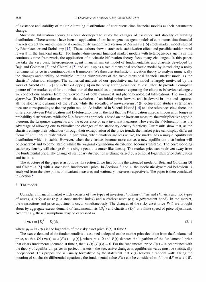
Fig. 5. Joint stationary densities of the price p and the assessment of the price trend ψ and the corresponding marginal distributions for p andψ-axis for a = 1, α = 2, β = 1, σ = 0.02.

size 0.001. Since the average amount of time this solution path spends in each sample set is approximately equal tothe measure of this set, we obtain a histogram as an estimation of the density of the stationary measure. For a bettervisualization, the density functions are then smoothed by using a standard procedure.

For a = 1, α = 2, β = 1, and σ = 0.02, Fig. 5 shows qualitatively different joint and marginal stationary densitiesfor the different c values of 0.5, 1, and 1.1. Fig. 5 shows the joint stationary densities (the first panel) and the marginaldensities (the second and third panels) for the variables p and ψ .

Note that there is a one-to-one correspondence between the stationary measure ρ and the invariant measure µωwhich is measurable with respect to the past F0

−∞ := σ(Ws, s ≤ 0) (the σ -algebra generated by Wss≤0). Thiscorrespondence is given by µω → Eµω = ρ and ρ → limt→∞ ϕ(t, ϑ−tω)ρ := µω (see Arnold [1]). Then combiningwith the analysis of D-bifurcation, we can see from Fig. 5 that, for c = 0.5, the joint densities in the (p, ψ) planeshave one peak and the marginal densities for either ψ or p are unimodal, which corresponds to the stable Diracinvariant measure µω = δx∗(ω) with the global random attractor A(ω) = x∗(ω) under the D-bifurcation analysis.However, for c = 1.1, the joint density in the (p, ψ) plane has a crater-like shape and the marginal densities foreither ψ or p are bimodal. This change is underlined by the stable Dirac invariant measure νω = δx∗(ω) with theglobal random attractor of a random disc under the D-bifurcation analysis. For c = 1, the joint (marginal) densitycan be regarded as the transition from single peak to crater-like (from unimodal to bimodal) density. Therefore, as thechartists’ adjustment parameter c increases, the qualitative changes of the stationary density indicates the occurrenceof a P-bifurcation.


5. Conclusion

This paper presents a continuous-time stochastic asset pricing model of a speculative financial market withfundamentalists and chartists. By applying stochastic bifurcation theory, we examine the limiting market equilibriumdistribution numerically. We have shown that speculative behaviour of chartists can lead the market price to displaydifferent forms of equilibrium distributions. We have demonstrated the combined analysis of both D- and P-bifurcations certainly gives us a relatively complete picture of the stochastic behaviour of our model. In particular,when the chartists extrapolate the trend weakly (so that c < cD), the system only has one invariant measure δx∗(ω)

which is stable. In this case, x∗(ω) has a stationary measure which has one peak. However, when the chartistsextrapolate the trend strongly (so that c > cD), a new stable random Dirac measure δx](ω) appears and thecorresponding stationary measure has a crater-like density. The change of stationary distribution is characterizedby a bimodal logarithm price distribution and fat tails.

To conclude the paper, we refer to Chiarella, He and Zheng [6] for more detailed analysis of the stochasticbifurcation of the fundamentalist-chartist model and the relationship between the stochastic and deterministicdynamics of the model. The cited paper provides more insights into the model of stochastic behaviour throughstochastic bifurcation analysis, stochastic approximation methods and the difference between deterministic andstochastic dynamics. It demonstrates that stochastic bifurcation analysis can be a powerful tool to help inunderstanding various types of financial market behaviour.

References

[1] L. Arnold, Random Dynamical Systems, Springer, New York, 1998.[2] L. Arnold, N. Sri Namachchivaya, K.R. Schenk-Hoppe, Towards an understanding of stochastic Hopf bifurcation: A case study, Int. J. Bifurcat.

Chaos 6 (1996) 1947–1975.[3] A. Beja, M.B. Goldman, On the dynamic behaviour of prices in disequilibrium, J. Finance 35 (1980) 235–248.[4] V. Bohm, C. Chiarella, Mean variance preferences, expectations formation, and the dynamics of random asset prices, Math. Finance 15 (2005)

61–97.[5] C. Chiarella, The dynamics of speculative behaviour, Ann. Oper. Res. 37 (1992) 101–123.[6] C. Chiarella, X. He, M. Zheng, The stochastic price dynamics of speculative behaviour, Working Paper, QFRC, University of Technology,

Sydney, 2007.[7] H. Crauel, F. Flandoli, Attractors for random dynamical systems, Probab. Theory Related Fields 100 (1994) 365–393.[8] H. Crauel, Invariant measures are supported by random attractors, 1995, preprint.[9] H. Follmer, U. Horst, A. Kirman, Equilibria in financial markets with heterogeneous agents: A probabilistic perspective, J. Math. Econom. 41

(2005) 123–155.[10] V.I. Oseledets, A multiplicative Ergodic theorem. Lyapunov characteristic numbers for dynamical systems, Trans. Moscow Math. Soc. 19

(1968) 197–231.[11] T.S. Parker, L.O. Chua, Practical Numerical Algorithms for Chaotic Systems, Springer-Verlag, New York, 1989.[12] T. Rheinlaender, M. Steinkamp, A stochastic version of Zeeman’s market model, Stud. Nonlinear Dynam. Econometrics 8 (2004) 1–23.[13] K.R. Schenk-Hoppe, Deterministic and stochastic Duffing–van der Pol oscillators are non-explosive, Z. Angew. Math. Phys. 47 (1996)

740–759.[14] K.R. Schenk-Hoppe, Bifurcation scenarios of the noisy Duffing–van der Pol oscillator, Nonlinear Dynam. 11 (1996) 255–274.[15] E. Zeeman, The unstable behavior of stock exchanges, J. Math. Econom. 1 (1974) 39–49.

the stochastic bifurcation behaviour of speculative financial markets

Documents