The Stability of Hot Spot Patterns forReaction-Diffusion Models of Urban

CrimeMichael J. Ward (UBC)

PIMS Hot Topics: Computational Criminology and UBC (IAM), September 2012

Joint With: Theodore Kolokolonikov (Dalhousie); Simon Tse (UBC); Juncheng Wei

(Chinese U. Hong Kong, UBC)

UBC – p. 1

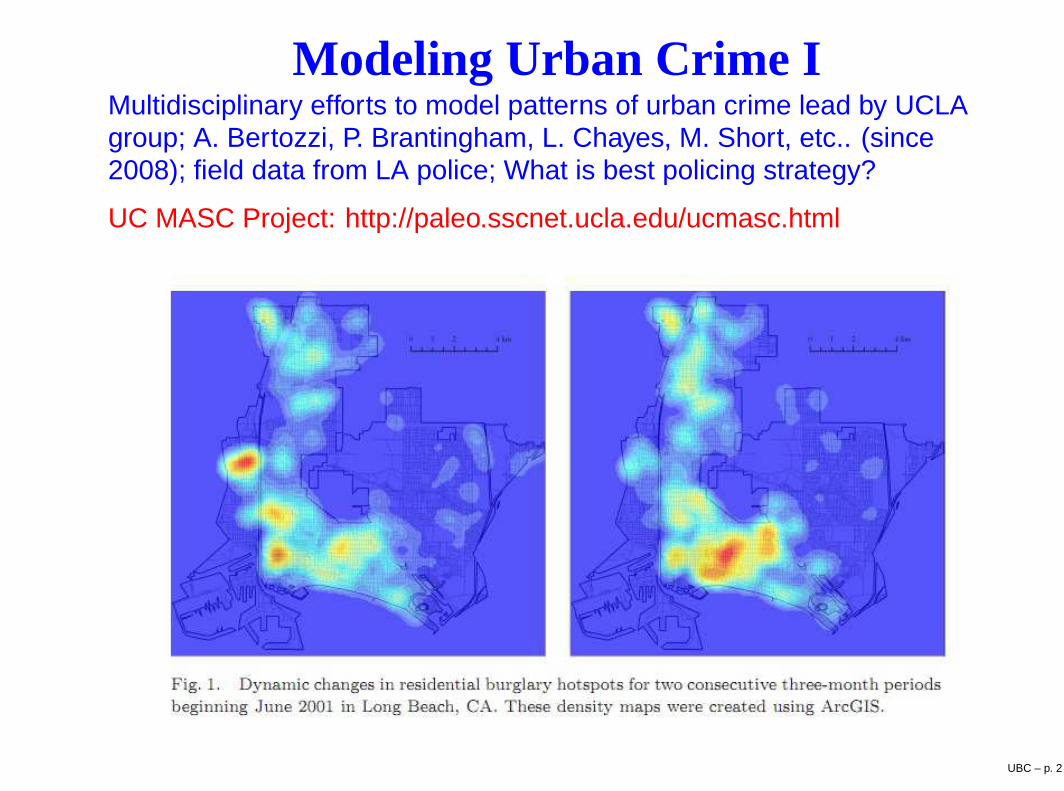
Modeling Urban Crime IMultidisciplinary efforts to model patterns of urban crime lead by UCLAgroup; A. Bertozzi, P. Brantingham, L. Chayes, M. Short, etc.. (since2008); field data from LA police; What is best policing strategy?

UC MASC Project: http://paleo.sscnet.ucla.edu/ucmasc.html

UBC – p. 2

Modeling Urban Crime II

Key References:

M. B. Short, P. J. Brantingham, A. L. Bertozzi and G. E. Tita (2010),Dissipation and displacement of hotpsots in reaction-diffusion modelsof crime, PNAS, 107(9) pp. 3961-3965. Made the cover of PNAS.

M. B. Short, M. R. D’Orsogna, V. B. Pasour, G. E. Tita,P. J. Brantingham, A. L. Bertozzi and L. B. Chayes (2008), A statisticalmodel of criminal behavior, M3AS, 18, Suppl. pp. 1249–1267.

M. B. Short, A. L. Bertozzi and P. J. Brantingham (2010), Nonlinearpatterns in urban crime - hotpsots, bifurcations, and suppression,SIADS, 9(2), pp. 462–483.

Observations: Criminal activity concentrates non-uniformly (good versusbad neighborhoods). Often “hot-spots” of crime are observed. Need toincorporate near-repeat victimization and elevated risk of re-victimizationin a short time period.

UBC – p. 3

An Agent-Based Model I

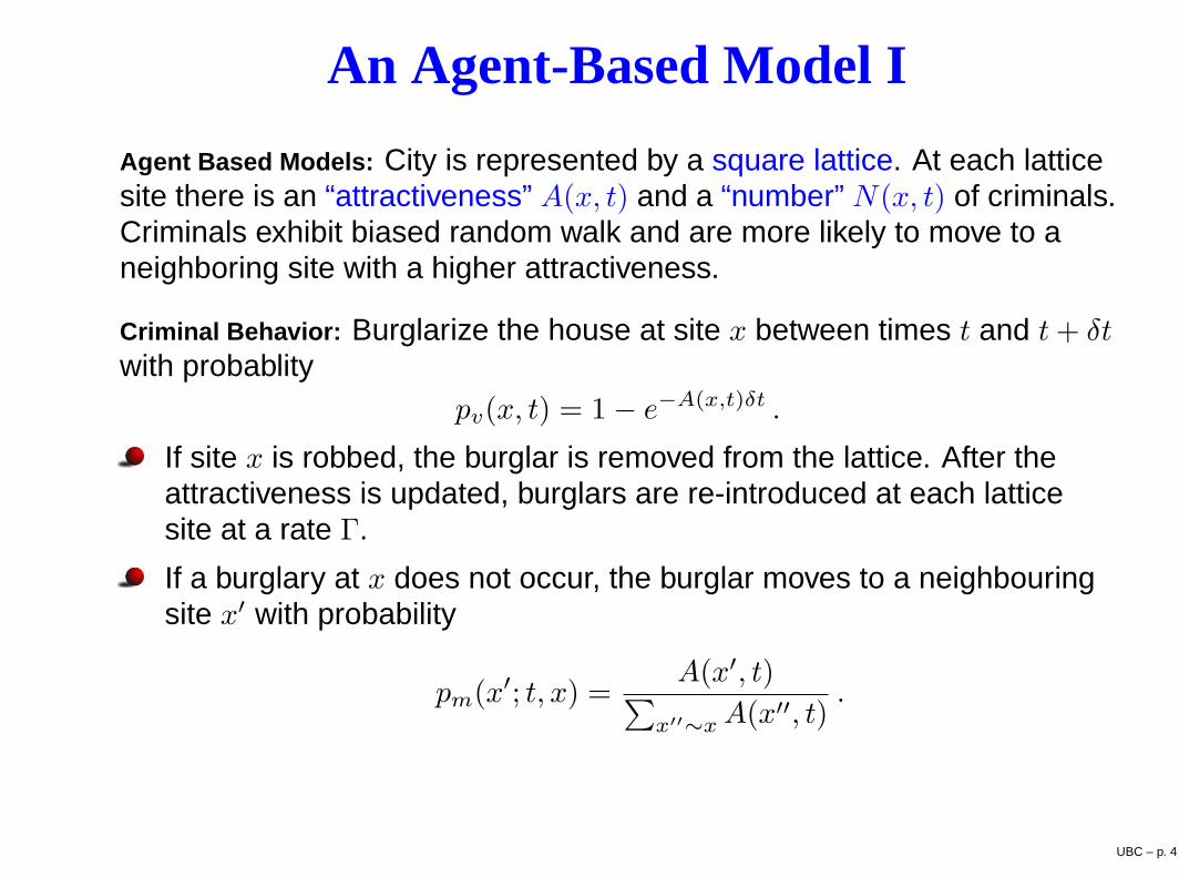
Agent Based Models: City is represented by a square lattice. At each latticesite there is an “attractiveness” A(x, t) and a “number” N(x, t) of criminals.Criminals exhibit biased random walk and are more likely to move to aneighboring site with a higher attractiveness.

Criminal Behavior: Burglarize the house at site x between times t and t+ δtwith probablity

pv(x, t) = 1− e−A(x,t)δt .

If site x is robbed, the burglar is removed from the lattice. After theattractiveness is updated, burglars are re-introduced at each latticesite at a rate Γ.

If a burglary at x does not occur, the burglar moves to a neighbouringsite x′ with probability

pm(x′; t, x) =A(x′, t)

∑

x′′∼xA(x′′, t)

.

UBC – p. 4

An Agent-Based Model IIModeling attractiveness: It has a static and dynamic component:

A(x, t) = A0 +B(x, t) .

Elevated risk of re-victimization in a short time-period with decay rate ωand with a parameter η ≪ 1 that models how attractiveness is spread toits neighbours:

B(x, t+ δt) =

[

(1− η)B(x, t) +η

4

∑

x′∼x

B(x′, t)

]

(1− ω δt) + θE(x, t) .

Here θ > 0 and E(x, t) is the number of burglary events at site x in a timeinterval (t, t+ δt). Then, update attractiveness

A(x, t+ δt) = A0 +B(x, t+ δt)

Remark: Expected value(E)= N(x, t)pv(x, t).

Numerics (Agent-Based): (stationary hot-spots, moving hot-spots, creation ofnew spots, etc..) Agent Based Simulation (M. Short et al:) (Movie)

UBC – p. 5

The Basic Urban RD Crime Model

In the continuum limit, the resulting dimensionless PDE RD model with noflux b.c. is (Short et al., M3AS, (2008)):

At = ε2∆A−A+ PA+ α , x ∈ Ω ,

τPt = D∇ ·(

∇P − 2P

A∇A

)

− PA+ γ − α , x ∈ Ω .

ε≪ 1 (results from η ≪ 1)

P (x, t) is criminal density; A(x, t) is “attractiveness” to burglary.

The chemotactic drift term −2D∇ ·(

P ∇AA

)

represents the tendency ofcriminals to move towards sites with a higher attractiveness.

Here α is the baseline attractiveness, while γ − α > 0 is the constantrate of re-introduction of criminals after a burglary.

The spatially homogeneous equilibrium state is

Pe = (γ − α)/γ , Ae = γ .

UBC – p. 6

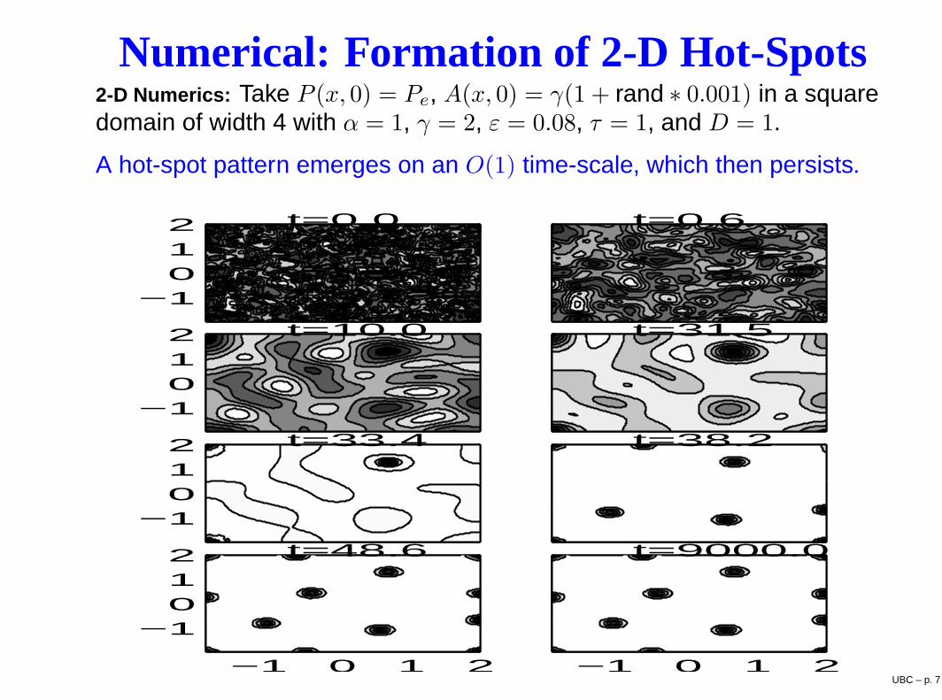
Numerical: Formation of 2-D Hot-Spots2-D Numerics: Take P (x, 0) = Pe, A(x, 0) = γ(1 + rand ∗ 0.001) in a squaredomain of width 4 with α = 1, γ = 2, ε = 0.08, τ = 1, and D = 1.

A hot-spot pattern emerges on an O(1) time-scale, which then persists.

−1012 t=0.0 t=0.6

−1012 t=10.0 t=31.5

−1012 t=33.4 t=38.2

−1 0 1 2

−1012 t=48.6

−1 0 1 2

t=9000.0

UBC – p. 7

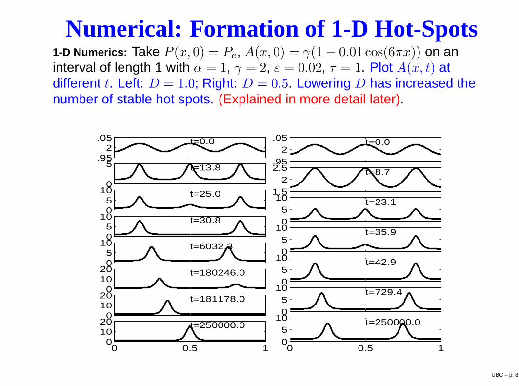
Numerical: Formation of 1-D Hot-Spots1-D Numerics: Take P (x, 0) = Pe, A(x, 0) = γ(1− 0.01 cos(6πx)) on aninterval of length 1 with α = 1, γ = 2, ε = 0.02, τ = 1. Plot A(x, t) atdifferent t. Left: D = 1.0; Right: D = 0.5. Lowering D has increased thenumber of stable hot spots. (Explained in more detail later).

1.952

2.05 t=0.0

0

5 t=13.8

05

10 t=25.0

05

10 t=30.8

05

10 t=6032.3

01020 t=180246.0

01020 t=181178.0

0 0.5 10

1020 t=250000.0

1.952

2.05 t=0.0

1.52

2.5 t=8.7

05

10 t=23.1

05

10 t=35.9

05

10 t=42.9

05

10 t=729.4

0 0.5 105

10 t=250000.0

UBC – p. 8

Outline and Perspective IMathematical Modeling Remarks:

Formulation: formulation of stochastic agent-based model based onobservational trends in crime, behavior of criminals, etc...... easy toincorporate many effects...

Age of Discovery: numerical realizations of the agent-based model toobserve qualitatively interesting phenomena (stationary hot-spots,moving hot-spots, creation of new spots, etc..)

Continuum Limit: Derivation of a “simpler” PDE reaction–diffusion (RD)system. Usual First Step: Numerical simulations of PDE system,Turing and weakly nonlinear analysis of patterns.....

Rigorous PDE Analysis: existence, regularity, and bifurcation-theoreticresults for the PDE model (Rodriguez, Cantrell, Cosner andManasevich).

Model Validation: matching model predictions with field observations.Improving the model. Developing new models (somegame-theoretic)... (Berestycki-Nadal, Pilcher, Short and D’Orsogna).

UBC – p. 9

Outline and Perspective IIHowever: many seemingly “simple-looking” RD systems can exhibitextremely complex dynamics in the nonlinear regime in differentparameter ranges; i.e witness the Gray-Scott model of chemical physics(1996–date).

Our Approach: For the RD model of urban crime, use a combination offormal asymptotics, rigorous analysis, and computation, to obtainanalytical results for stability thresholds, delineating in parameter spacewhere different solution behaviors occur, etc...

Specific Goal: Analyze the existence and stability of localized patterns ofcriminal activity for this model in the limit ε→ 0. We also considerextensions of the basic model to include the effect of “police”. Thesepatterns are “far-from-equilibrium” (Y. Nishiura..), and not amenable tostandard Turing stability analysis.

Particle-like solutions to PDE’s; vortices, skyrmions, ho t-spots, ...

UBC – p. 10

Turing-Stability AnalysisThe uniform state Ae, Pe on R

1 is unstable for ε→ 0 when γ > 3α/2. Withan eimx+λt perturbation, the Turing instability band is

D−1/2γ(2γ − 3α)−1/2 ∼ mlower < m < mupper ∼ ε−1γ−1/2(2γ − 3α)1/2 .

For ε→ 0, the maximum growth rate is λmax ∼ O(1), with the mostunstable mode

mmax ∼ ε−1/2D−1/4γ−1/2[

(γ − α)(3γ2 + 2τ(2γ − 3α)]1/4

.

Remark 1: For perturbations of the uniform state the preferred pattern has acharacteristic half-length lturing ∼ π/mmax, where

lturing ∼ ε1/2D1/4γ1/2[

(γ − α)(3γ2 + 2τ(2γ − 3α))]−1/4

π .

Notice that lturing = O(1) when D = O(ε−2).

Remark 2: Turing and weakly nonlinear analysis in 1-D and 2-D given inShort et al. (SIADS 2010), together with full numerical computations.

UBC – p. 11

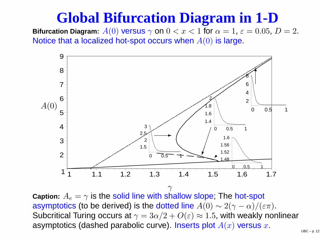
Global Bifurcation Diagram in 1-DBifurcation Diagram: A(0) versus γ on 0 < x < 1 for α = 1, ε = 0.05, D = 2.Notice that a localized hot-spot occurs when A(0) is large.

1

2

3

4

5

6

7

8

9

1 1.1 1.2 1.3 1.4 1.5 1.6 1.7

2

4

6

8

0 0.5 1

1.4

1.6

1.8

2

0 0.5 1

1.48

1.52

1.56

1.6

0 0.5 1

1.52

2.53

0 0.5 1

-

6

γ

A(0)

Caption: Ae = γ is the solid line with shallow slope; The hot-spotasymptotics (to be derived) is the dotted line A(0) ∼ 2(γ − α)/(επ).Subcritical Turing occurs at γ = 3α/2 +O(ε) ≈ 1.5, with weakly nonlinearasymptotics (dashed parabolic curve). Inserts plot A(x) versus x.

UBC – p. 12

Basic RD Crime Model: Qualitative IThere are two key parameter regimes: D ≫ 1 and D = O(1)

Regime 1: D ≫ 1

Localized patterns in the form of pulses or spikes are readilyconstructed using singular perturbation techniques for the regimeO(1) ≪ D ≤ O(ε−2) in 1-D and O(1) ≪ D ≤ O(ε−4) in 2-D.

The stability threshold for these patterns occurs when D = O(ε−2) in1-D and D = O(ε−4) in 2-D.

The stability theory is based primarily on an exactly solvable nonlocaleigenvalue problem.

A further stability threshold in D with respect to instabilities developingover a long time scale t = O(ε−2) must also be calculated.

Implication: The stability threshold in terms of D determines the mininumspacing between localized elevated regions of criminal activity that allowsfor a stable pattern, i.e. If Dcrit is large, stable hot-spots are closelyspaced.

UBC – p. 13

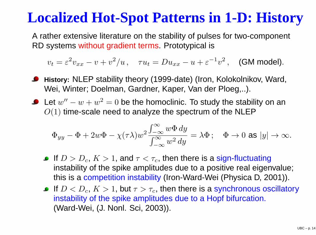
Localized Hot-Spot Patterns in 1-D: HistoryA rather extensive literature on the stability of pulses for two-componentRD systems without gradient terms. Prototypical is

vt = ε2vxx − v + v2/u , τut = Duxx − u+ ε−1v2 , (GM model).

History: NLEP stability theory (1999-date) (Iron, Kolokolnikov, Ward,Wei, Winter; Doelman, Gardner, Kaper, Van der Ploeg,..).

Let w′′ − w + w2 = 0 be the homoclinic. To study the stability on anO(1) time-scale need to analyze the spectrum of the NLEP

Φyy − Φ+ 2wΦ− χ(τλ)w2

∫∞

−∞wΦ dy

∫∞

−∞w2 dy

= λΦ ; Φ → 0 as |y| → ∞.

If D > Dc, K > 1, and τ < τc, then there is a sign-fluctuatinginstability of the spike amplitudes due to a positive real eigenvalue;this is a competition instability (Iron-Ward-Wei (Physica D, 2001)).If D < Dc, K > 1, but τ > τc, then there is a synchronous oscillatoryinstability of the spike amplitudes due to a Hopf bifurcation.(Ward-Wei, (J. Nonl. Sci, 2003)).

UBC – p. 14

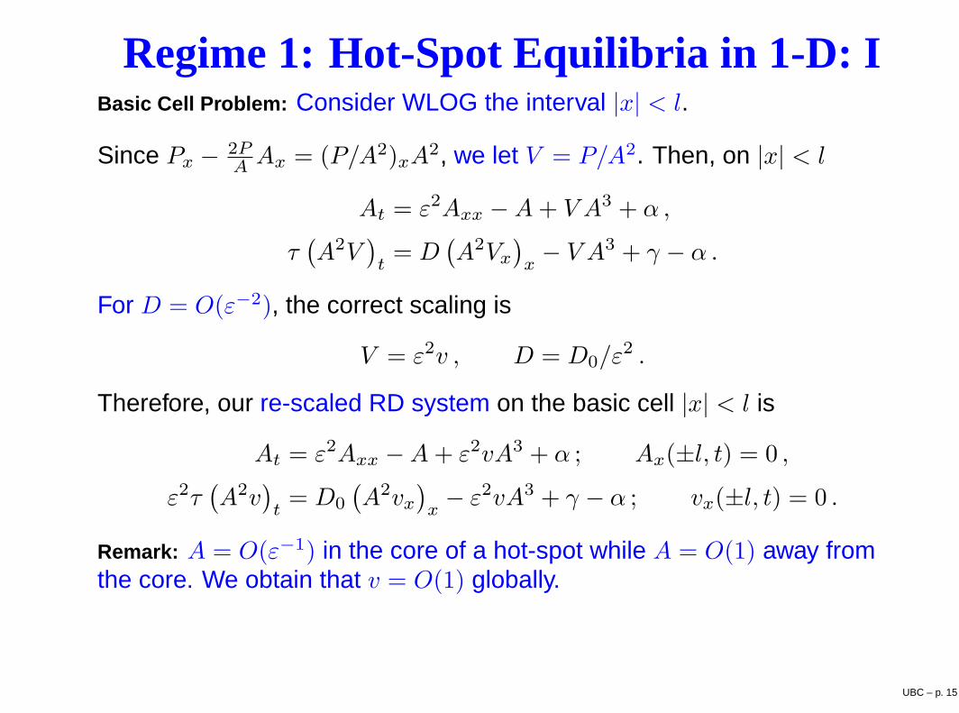
Regime 1: Hot-Spot Equilibria in 1-D: IBasic Cell Problem: Consider WLOG the interval |x| < l.

Since Px − 2PA Ax = (P/A2)xA

2, we let V = P/A2. Then, on |x| < l

At = ε2Axx −A+ V A3 + α ,

τ(

A2V)

t= D

(

A2Vx)

x− V A3 + γ − α .

For D = O(ε−2), the correct scaling is

V = ε2v , D = D0/ε2 .

Therefore, our re-scaled RD system on the basic cell |x| < l is

At = ε2Axx −A+ ε2vA3 + α ; Ax(±l, t) = 0 ,

ε2τ(

A2v)

t= D0

(

A2vx)

x− ε2vA3 + γ − α ; vx(±l, t) = 0 .

Remark: A = O(ε−1) in the core of a hot-spot while A = O(1) away fromthe core. We obtain that v = O(1) globally.

UBC – p. 15

Regime 1: Hot-Spot Equilibria in 1-D: IIFrom a matched asymptotic analysis:

Principal Result: Let ε→ 0 and O(1) ≪ D ≤ O(ε−2) with D0 ≡ ε2D. Then,for a one-hot-spot solution centered at x = 0 on |x| ≤ l, the leading-orderuniform asymptotics for A and P are

A ∼ 1√2

(

2l(γ − α)

πε− α

)

w(x/ε) + α , P ∼ [w(x/ε)]2.

Here w(y) =√2sech (y) is the homoclinic of w′′ − w + w3 = 0. The inner

and outer approximations for v are

v ∼ v0+εv1 , |x| = O(ε) ; v ∼ ζ

2

(

(l − |x|)2 − l2)

+v0 , O(ε) < |x| < l ,

Here ζ ≡ (α− γ)/(D0α2) < 0 and v0 = π2

[

2l2(γ − α)2]−1

.

Remarks:

A(0) ∼ 2(γ − α)/(επ), as plotted previously on bifurcation diagram.

For a symmetric K-hot-spot pattern with spots of equal height on adomain of length S, simply set l = S/2K and use gluing.

UBC – p. 16

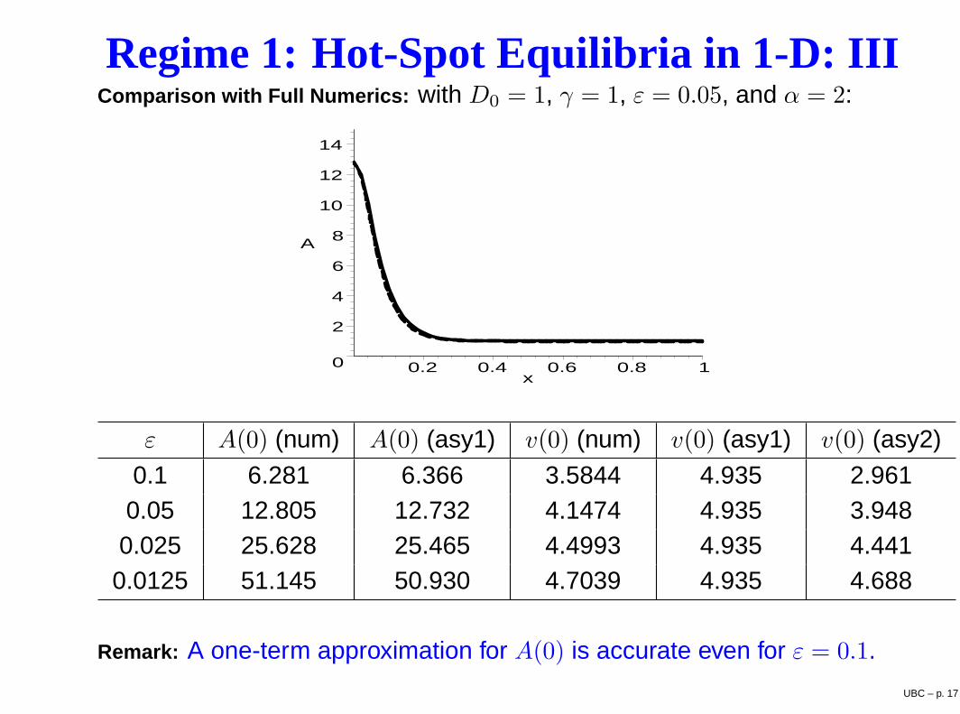
Regime 1: Hot-Spot Equilibria in 1-D: IIIComparison with Full Numerics: with D0 = 1, γ = 1, ε = 0.05, and α = 2:

0

2

4

6

8

10

12

14

A

0.2 0.4 0.6 0.8 1x

ε A(0) (num) A(0) (asy1) v(0) (num) v(0) (asy1) v(0) (asy2)

0.1 6.281 6.366 3.5844 4.935 2.9610.05 12.805 12.732 4.1474 4.935 3.948

0.025 25.628 25.465 4.4993 4.935 4.4410.0125 51.145 50.930 4.7039 4.935 4.688

Remark: A one-term approximation for A(0) is accurate even for ε = 0.1.

UBC – p. 17

NLEP Stability Analysis: ILet Ae, ve be one-spike solution on the basic cell |x| < l. We introduce

A = Ae + φeλt , v = ve + εψeλt .

The singularly perturbed eigenvalue problem is

ε2φxx − φ+ 3ε2veA2eφ+ ε3A3

eψ = λφ ,

D0

(

εA2eψx + 2Aevexφ

)

x− 3ε2A2

eveφ− ε3ψA3e = λτε2

(

εA2eψ + 2Aeveφ

)

.

For z complex, we impose the Floquet boundary conditions

φ(l) = zφ(−l) , φ′(l) = zφ′(−l) , ψ(l) = zψ(−l) , ψ′(l) = zψ′(−l) ,

To obtain the spectrum of a K-spike pattern on a domain of length 2Klsubject to periodic boundary conditions we set zK = 1, so that

zj = e2πij/K , j = 0, . . . ,K − 1 .

Remark: An NLEP is derived for the periodic b.c. problem by usingasymptotics to determine jump conditions for ψ across x = 0. Then, theNeumann spectra is extracted from Periodic spectra.

UBC – p. 18

NLEP Stability Analysis: IIAn asymptotic analysis shows that φ ∼ Φ(y) with y = ε−1x, where Φ(y) on−∞ < y <∞ satisfies

L0Φ ≡ Φ′′ − Φ+ 3w2Φ = −v−3/20 w3ψ(0) + λΦ ; Φ → 0 as |y| → ∞.

Then, for τ = O(1), ψ(0) is determined from

ψxx = 0 , 0 < |x| ≤ l ; ψ(l) = zψ(−l) , ψ′(l) = zψ′(−l) ,

subject to ψ(0+) = ψ(0−) ≡ ψ(0) and the jump condition across x = 0:

a0 [ψx]0 + a1ψ(0) = a2 ;

a0 ≡ D0α2 , a1 = −v−3/2

0

∫ ∞

−∞

w3 dy a2 = 3

∫ ∞

−∞

w2Φ dy

Remark: ψ(0) involves one nonlocal term.

UBC – p. 19

NLEP Stability Analysis: IIIPrincipal Result: Consider a K > 1 equilibrium hot-spots on an interval oflength S with no-flux conditions. For ε→ 0, τ = O(1), and with D0 = ε2D,the stability of this solution with respect to the “large” eigenvaluesλ = O(1) of the linearization is determined by the spectrum of the NLEP

L0Φ− χjw3

∫∞

−∞w2Φ dy

∫∞

−∞w3 dy

= λΦ ; Φ → 0 as |y| → ∞ ,

χj = 3

[

1 +D0α

2π2K4

4(γ − α)3

(

2

S

)4

(1− cos (πj/K))

]−1

, j = 0, . . . ,K − 1.

For K = 1 we have χ0 = 3. Here L0 (local operator) is

L0Φ ≡ Φ′′ − Φ+ 3w2Φ

Remark: In contrast to the NLEP’s for the GM and GS models, the discretespectrum for this NLEP is explicitly available.

UBC – p. 20

NLEP Stability Analysis: IVLemma: Let c be real, and consider the NLEP on −∞ < y <∞:

L0Φ− cw3

∫ ∞

−∞

w2Φ dy = λΦ ; Φ → 0 as |y| → ∞ ,

corresponding to∫∞

−∞w2Φ dy 6= 0. On the range Re(λ) > −1, there is a

unique discrete eigenvalue given by

λ = 3− c

∫ ∞

−∞

w5 dy .

Thus, λ is real and λ < 0 when c > 3/∫

w5 dy.

Idea of Proof: We use the key identity L0w2 = 3w2 and Green’s theorem

∫∞

−∞

(

w2L0Φ− ΦL0w2)

dy = 0 with L0Φ = cw3∫∞

−∞w2Φ dy + λΦ. Thus,

(

λ− 3 + c

∫ ∞

−∞

w5 dy

)∫ ∞

−∞

w2Φ dy = 0 ,

which yields the result.

UBC – p. 21

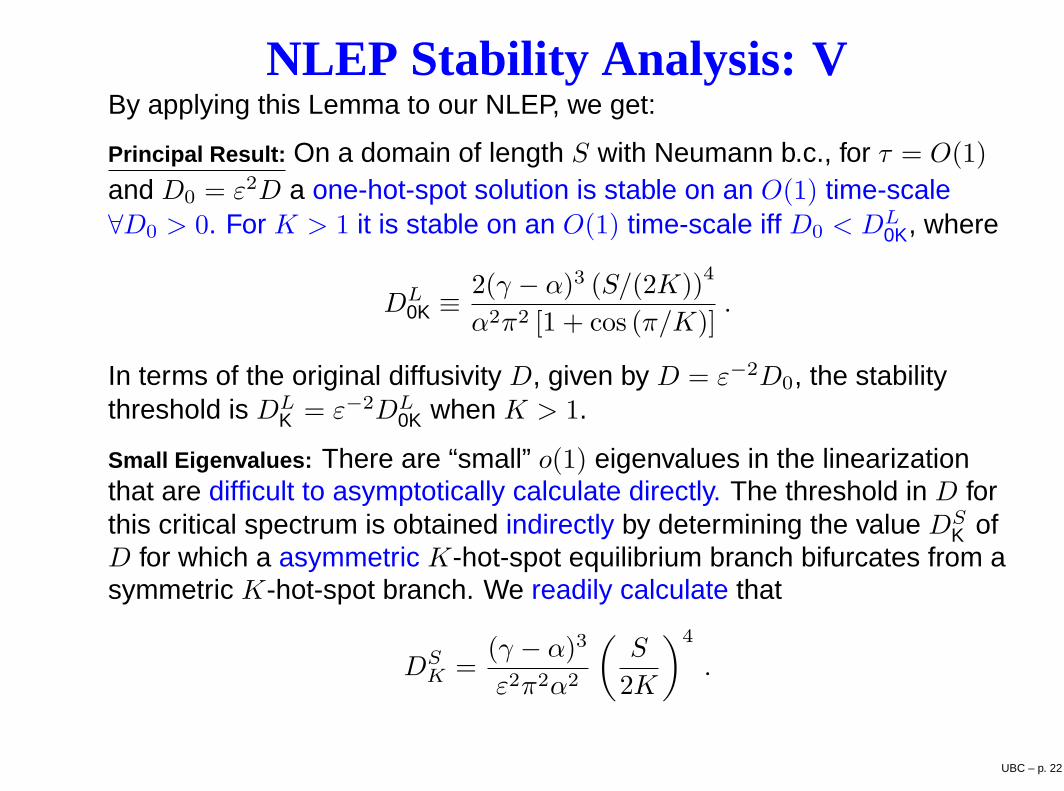
NLEP Stability Analysis: VBy applying this Lemma to our NLEP, we get:

Principal Result: On a domain of length S with Neumann b.c., for τ = O(1)

and D0 = ε2D a one-hot-spot solution is stable on an O(1) time-scale∀D0 > 0. For K > 1 it is stable on an O(1) time-scale iff D0 < DL

0K, where

DL0K ≡ 2(γ − α)3 (S/(2K))

4

α2π2 [1 + cos (π/K)].

In terms of the original diffusivity D, given by D = ε−2D0, the stabilitythreshold is DL

K = ε−2DL0K when K > 1.

Small Eigenvalues: There are “small” o(1) eigenvalues in the linearizationthat are difficult to asymptotically calculate directly. The threshold in D forthis critical spectrum is obtained indirectly by determining the value DS

K ofD for which a asymmetric K-hot-spot equilibrium branch bifurcates from asymmetric K-hot-spot branch. We readily calculate that

DSK =

(γ − α)3

ε2π2α2

(

S

2K

)4

.

UBC – p. 22

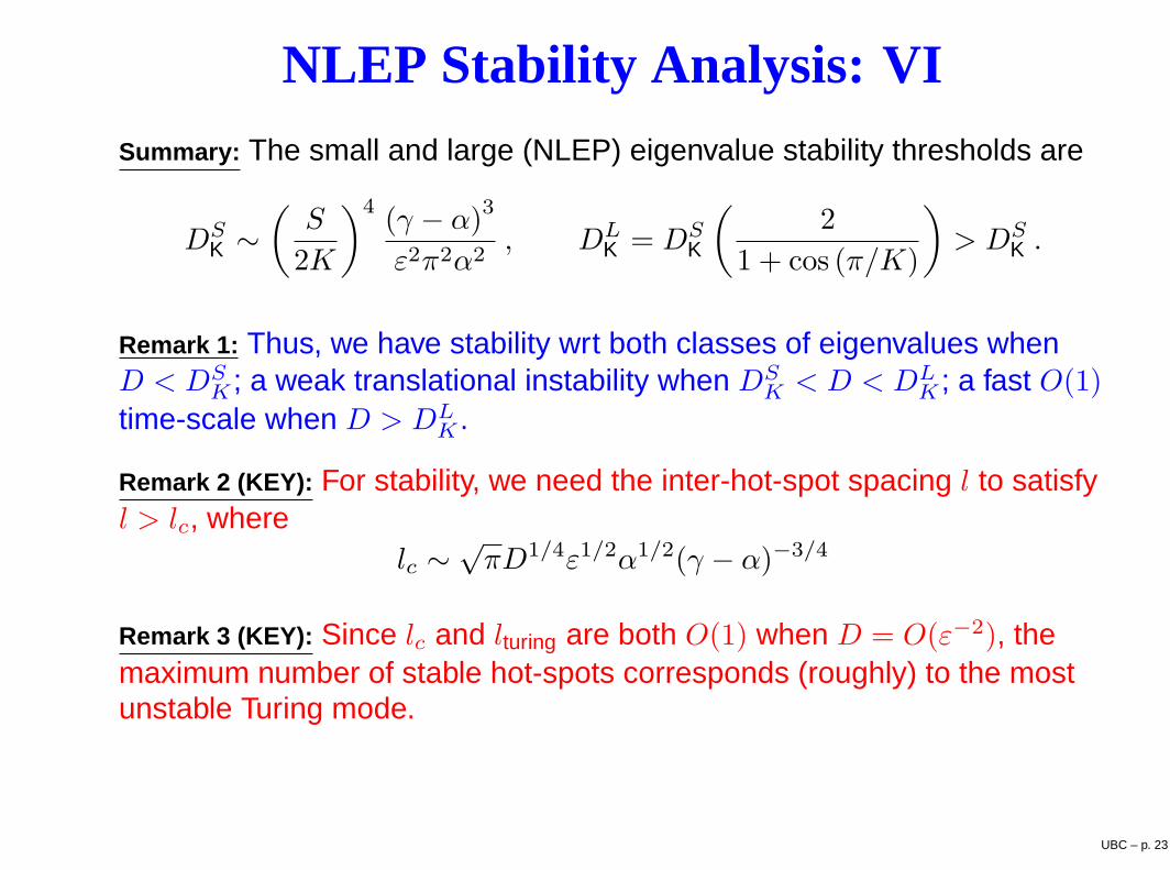
NLEP Stability Analysis: VISummary: The small and large (NLEP) eigenvalue stability thresholds are

DSK ∼

(

S

2K

)4(γ − α)

3

ε2π2α2, DL

K = DSK

(

2

1 + cos (π/K)

)

> DSK .

Remark 1: Thus, we have stability wrt both classes of eigenvalues whenD < DS

K ; a weak translational instability when DSK < D < DL

K ; a fast O(1)

time-scale when D > DLK .

Remark 2 (KEY): For stability, we need the inter-hot-spot spacing l to satisfyl > lc, where

lc ∼√πD1/4ε1/2α1/2(γ − α)−3/4

Remark 3 (KEY): Since lc and lturing are both O(1) when D = O(ε−2), themaximum number of stable hot-spots corresponds (roughly) to the mostunstable Turing mode.

UBC – p. 23

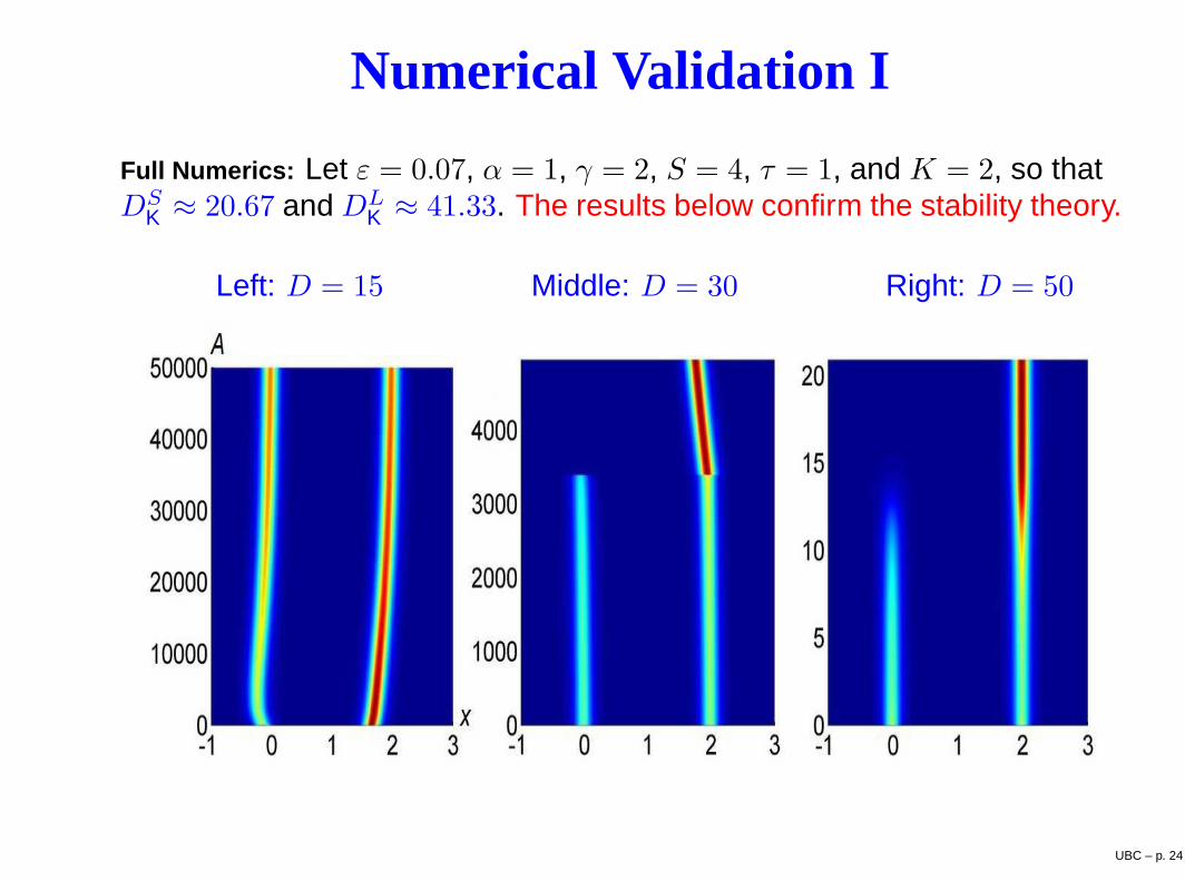
Numerical Validation I

Full Numerics: Let ε = 0.07, α = 1, γ = 2, S = 4, τ = 1, and K = 2, so thatDS

K ≈ 20.67 and DLK ≈ 41.33. The results below confirm the stability theory.

Left: D = 15 Middle: D = 30 Right: D = 50

UBC – p. 24

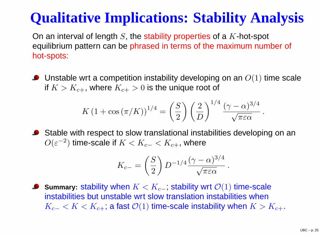
Qualitative Implications: Stability AnalysisOn an interval of length S, the stability properties of a K-hot-spotequilibrium pattern can be phrased in terms of the maximum number ofhot-spots:

Unstable wrt a competition instability developing on an O(1) time scaleif K > Kc+, where Kc+ > 0 is the unique root of

K (1 + cos (π/K))1/4

=

(

S

2

)(

2

D

)1/4(γ − α)3/4√

πεα.

Stable with respect to slow translational instabilities developing on anO(ε−2) time-scale if K < Kc− < Kc+, where

Kc− =

(

S

2

)

D−1/4 (γ − α)3/4√πεα

.

Summary: stability when K < Kc−; stability wrt O(1) time-scaleinstabilities but unstable wrt slow translation instabilities whenKc− < K < Kc+; a fast O(1) time-scale instability when K > Kc+.

UBC – p. 25

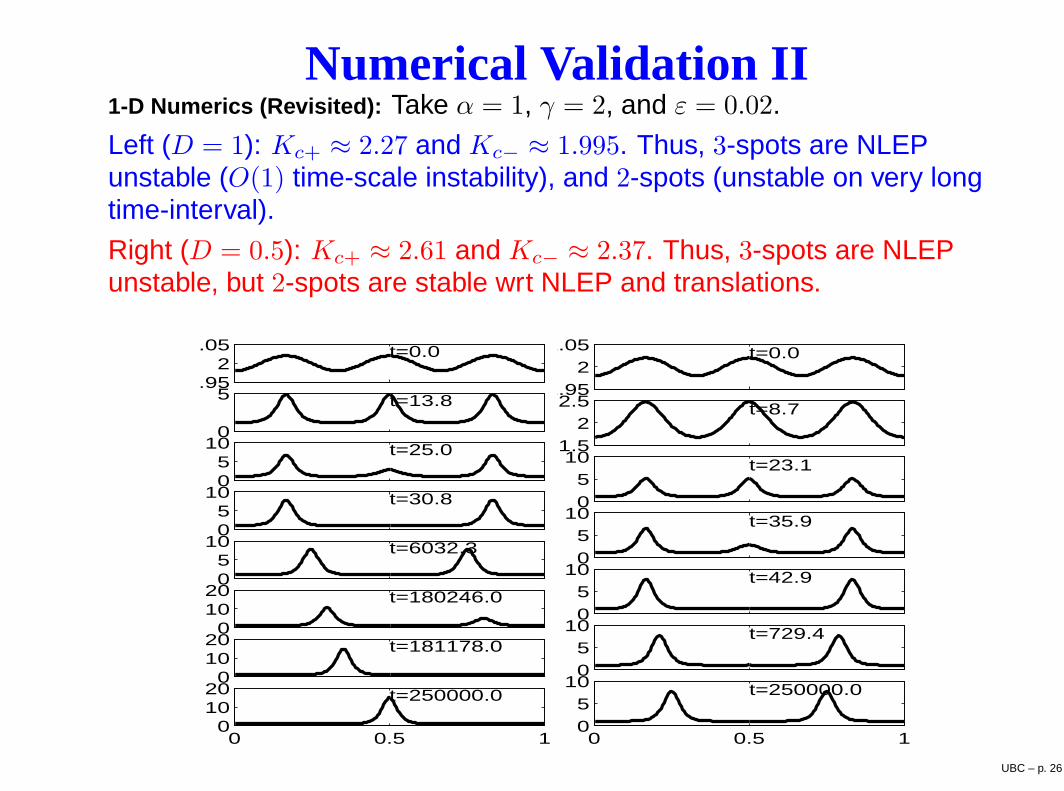
Numerical Validation II1-D Numerics (Revisited): Take α = 1, γ = 2, and ε = 0.02.

Left (D = 1): Kc+ ≈ 2.27 and Kc− ≈ 1.995. Thus, 3-spots are NLEPunstable (O(1) time-scale instability), and 2-spots (unstable on very longtime-interval).

Right (D = 0.5): Kc+ ≈ 2.61 and Kc− ≈ 2.37. Thus, 3-spots are NLEPunstable, but 2-spots are stable wrt NLEP and translations.

1.952

2.05 t=0.0

0

5 t=13.8

05

10 t=25.0

05

10 t=30.8

05

10 t=6032.3

01020 t=180246.0

01020 t=181178.0

0 0.5 10

1020 t=250000.0

1.952

2.05 t=0.0

1.52

2.5 t=8.7

05

10 t=23.1

05

10 t=35.9

05

10 t=42.9

05

10 t=729.4

0 0.5 105

10 t=250000.0

UBC – p. 26

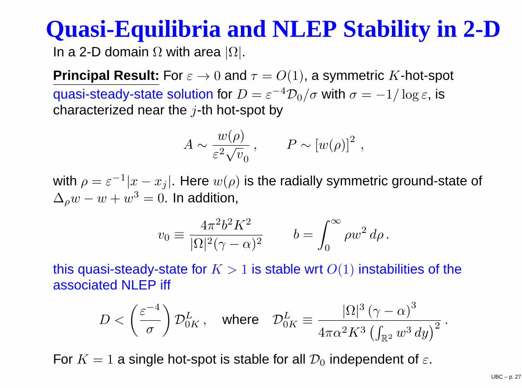
Quasi-Equilibria and NLEP Stability in 2-DIn a 2-D domain Ω with area |Ω|.Principal Result: For ε→ 0 and τ = O(1), a symmetric K-hot-spotquasi-steady-state solution for D = ε−4D0/σ with σ = −1/ log ε, ischaracterized near the j-th hot-spot by

A ∼ w(ρ)

ε2√v0, P ∼ [w(ρ)]

2,

with ρ = ε−1|x− xj |. Here w(ρ) is the radially symmetric ground-state of∆ρw − w + w3 = 0. In addition,

v0 ≡ 4π2b2K2

|Ω|2(γ − α)2b =

∫ ∞

0

ρw2 dρ .

this quasi-steady-state for K > 1 is stable wrt O(1) instabilities of theassociated NLEP iff

D <

(

ε−4

σ

)

DL0K , where DL

0K ≡ |Ω|3 (γ − α)3

4πα2K3(∫

R2 w3 dy)2 .

For K = 1 a single hot-spot is stable for all D0 independent of ε.UBC – p. 27

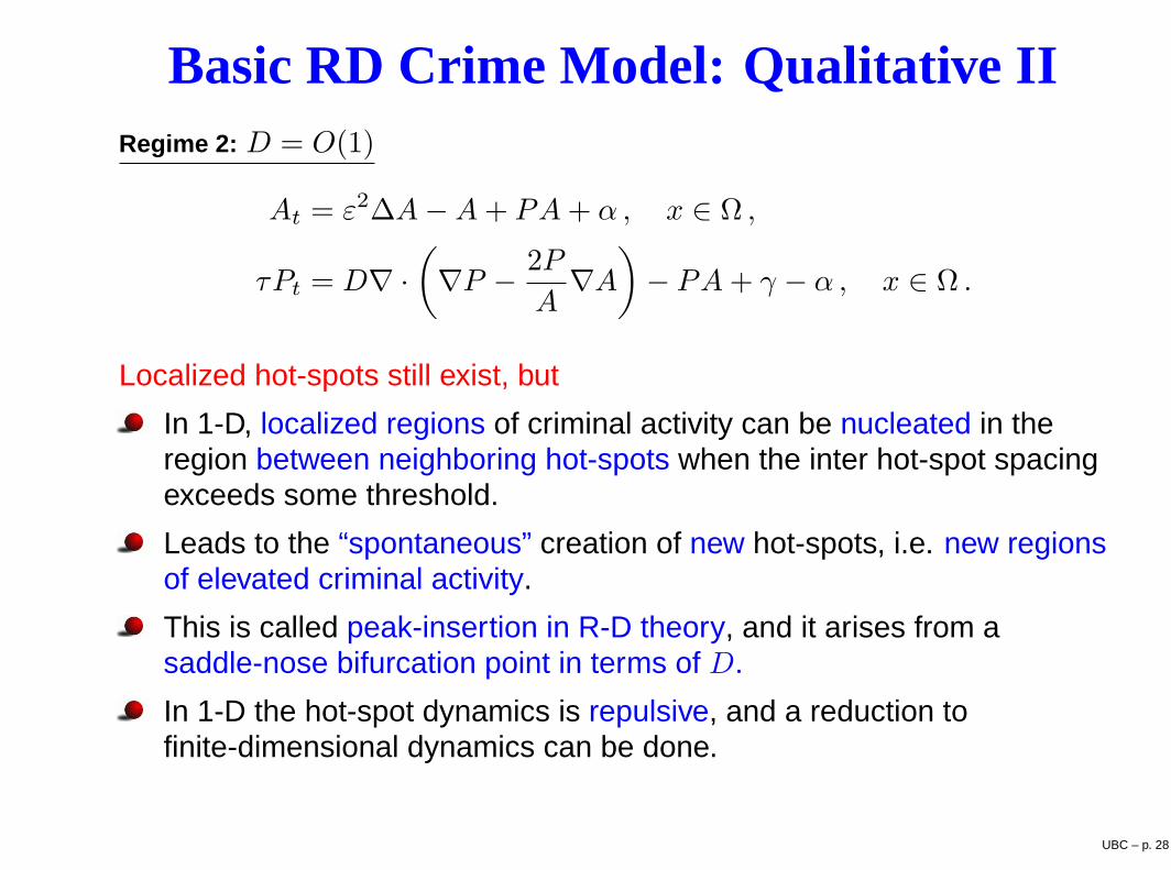
Basic RD Crime Model: Qualitative IIRegime 2: D = O(1)

At = ε2∆A−A+ PA+ α , x ∈ Ω ,

τPt = D∇ ·(

∇P − 2P

A∇A

)

− PA+ γ − α , x ∈ Ω .

Localized hot-spots still exist, but

In 1-D, localized regions of criminal activity can be nucleated in theregion between neighboring hot-spots when the inter hot-spot spacingexceeds some threshold.

Leads to the “spontaneous” creation of new hot-spots, i.e. new regionsof elevated criminal activity.

This is called peak-insertion in R-D theory, and it arises from asaddle-nose bifurcation point in terms of D.

In 1-D the hot-spot dynamics is repulsive, and a reduction tofinite-dimensional dynamics can be done.

UBC – p. 28

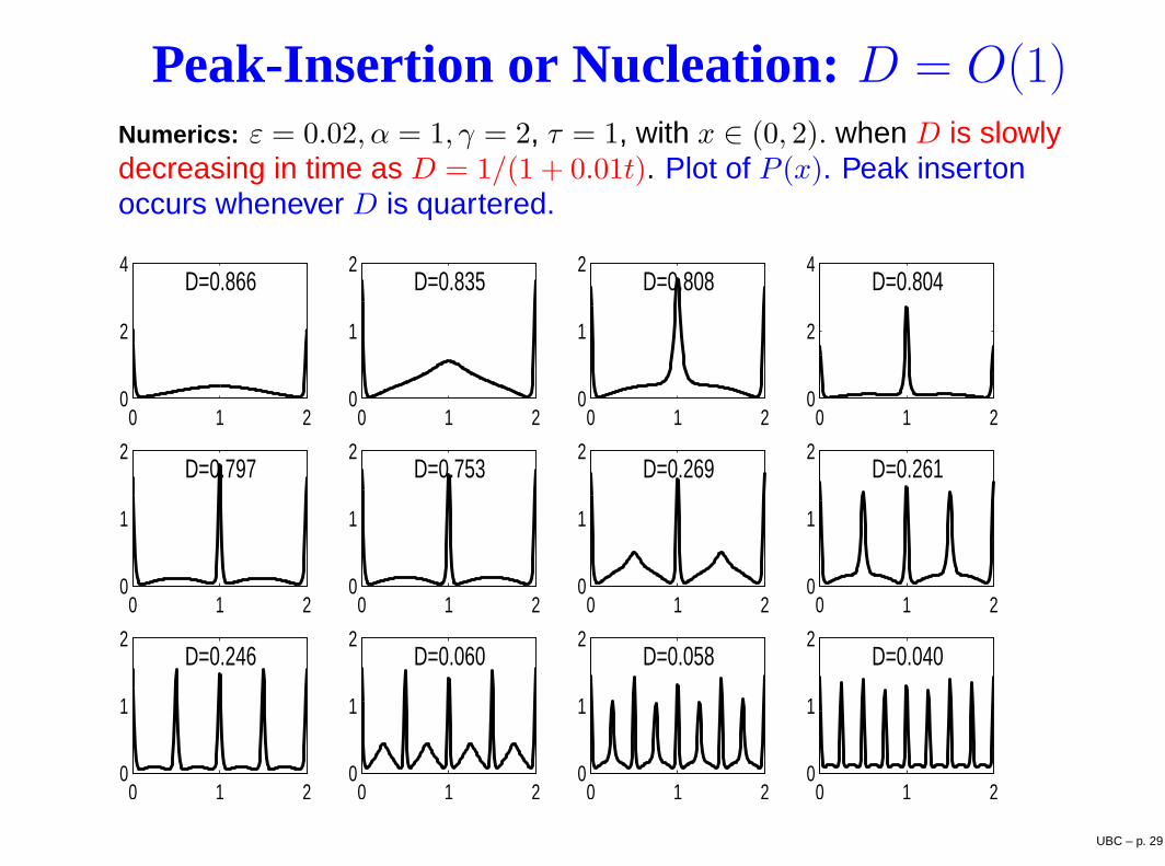
Peak-Insertion or Nucleation: D = O(1)Numerics: ε = 0.02, α = 1, γ = 2, τ = 1, with x ∈ (0, 2). when D is slowlydecreasing in time as D = 1/(1 + 0.01t). Plot of P (x). Peak insertonoccurs whenever D is quartered.

0 1 20

2

4D=0.866

0 1 20

1

2D=0.835

0 1 20

1

2D=0.808

0 1 20

2

4D=0.804

0 1 20

1

2D=0.797

0 1 20

1

2D=0.753

0 1 20

1

2D=0.269

0 1 20

1

2D=0.261

0 1 20

1

2D=0.246

0 1 20

1

2D=0.060

0 1 20

1

2D=0.058

0 1 20

1

2D=0.040

UBC – p. 29

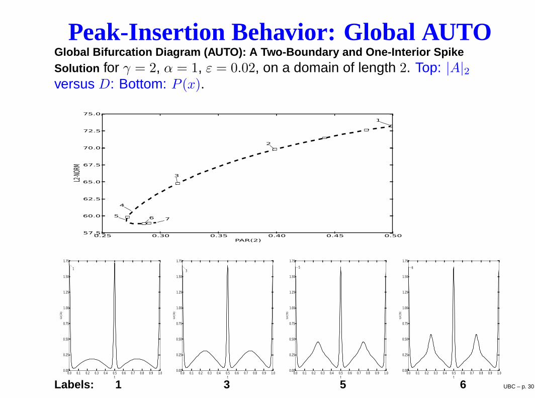
Peak-Insertion Behavior: Global AUTOGlobal Bifurcation Diagram (AUTO): A Two-Boundary and One- Interior SpikeSolution for γ = 2, α = 1, ε = 0.02, on a domain of length 2. Top: |A|2versus D: Bottom: P (x).

0.25 0.30 0.35 0.40 0.45 0.50PAR(2)

57.5

60.0

62.5

65.0

67.5

70.0

72.5

75.0

L2-NO

RM

1

2

3

4

5 6 7

0.0 0.1 0.2 0.3 0.4 0.5 0.6 0.7 0.8 0.9 1.0t

0.00

0.25

0.50

0.75

1.00

1.25

1.50

1.75

U(3)

1

0.0 0.1 0.2 0.3 0.4 0.5 0.6 0.7 0.8 0.9 1.0t

0.00

0.25

0.50

0.75

1.00

1.25

1.50

1.75

U(3)

3

0.0 0.1 0.2 0.3 0.4 0.5 0.6 0.7 0.8 0.9 1.0t

0.00

0.25

0.50

0.75

1.00

1.25

1.50

1.75

U(3)

5

0.0 0.1 0.2 0.3 0.4 0.5 0.6 0.7 0.8 0.9 1.0t

0.00

0.25

0.50

0.75

1.00

1.25

1.50

1.75

U(3)

6

Labels: 1 3 5 6 UBC – p. 30

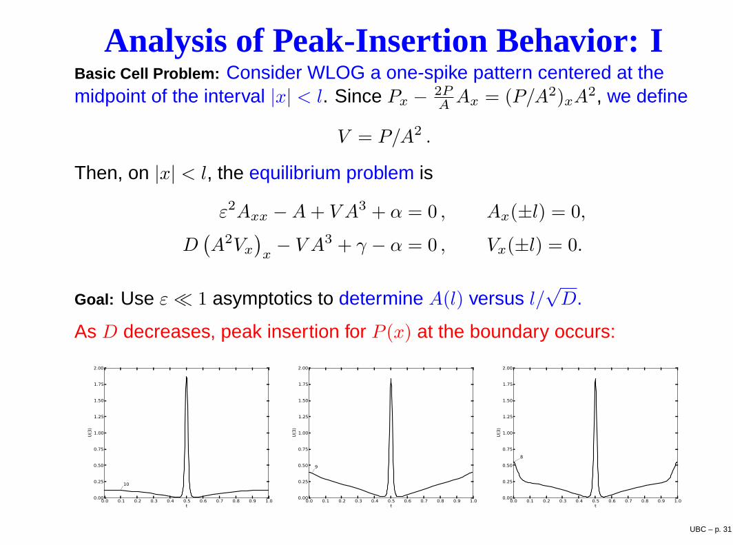
Analysis of Peak-Insertion Behavior: IBasic Cell Problem: Consider WLOG a one-spike pattern centered at themidpoint of the interval |x| < l. Since Px − 2P

A Ax = (P/A2)xA2, we define

V = P/A2 .

Then, on |x| < l, the equilibrium problem is

ε2Axx −A+ V A3 + α = 0 , Ax(±l) = 0,

D(

A2Vx)

x− V A3 + γ − α = 0 , Vx(±l) = 0.

Goal: Use ε≪ 1 asymptotics to determine A(l) versus l/√D.

As D decreases, peak insertion for P (x) at the boundary occurs:

0.0 0.1 0.2 0.3 0.4 0.5 0.6 0.7 0.8 0.9 1.0t

0.00

0.25

0.50

0.75

1.00

1.25

1.50

1.75

2.00

U(3)

10

0.0 0.1 0.2 0.3 0.4 0.5 0.6 0.7 0.8 0.9 1.0t

0.00

0.25

0.50

0.75

1.00

1.25

1.50

1.75

2.00

U(3)

9

0.0 0.1 0.2 0.3 0.4 0.5 0.6 0.7 0.8 0.9 1.0t

0.00

0.25

0.50

0.75

1.00

1.25

1.50

1.75

2.00

U(3)

8

UBC – p. 31

Analysis of Peak-Insertion Behavior: IIInner Region: We set y = x/ε, and expand

A ∼ ε−1A0 +A1 + · · · , V ∼ ε2v0 + · · ·

We obtain thatA0 = w/

√

v0 , w =√2sech(y) ,

where w′′ − w + w3 = 0. Here v0 is to be found, and A1 → α as y → ±∞.

Outer Region: WLOG consider 0+ < x ≤ l. Key: The leading order outerproblem is nonlinear. With, A ∼ a0 and V ∼ v0, then

v0a30 = a0 − α , D

(

a20v0x)

x= v0a

30 − (γ − α) ,

which leads to

D (f(a0)a0x)x = a0 − γ , 0 < x ≤ l ; a0(0+) = α , a0x(l) = 0 ,

wheref(a0) ≡ a−2

0 (3α− 2a0) .

UBC – p. 32

Analysis of Peak-Insertion Behavior: IIIRemark 1: We have f(a0) > 0 and a0x > 0 when a0 < 3α/2 < γ. Note: forγ > 3α/2 the spatially homogeneous steady-state is Turing unstable.

Remark 2: For the existence of a solution a0 we require a0(l) ≡ µ ≤ 3α/2.

Upon integrating the BVP for a0, we obtain an implicit relation for µ ≡ a0(l)

in terms of l/√D. Namely,

√

2

Dl = χ(µ) ≡ 2

γ − α

√

G(α;µ) + 2

∫ µ

α

1

(η − γ)2

√

G(η;µ) dη ,

where

G(η;µ) ≡∫ µ

η

f(s)(γ−s) ds = 2(µ−η)−(2γ+3α) log

(

µ

η

)

+3αγ

(

1

η− 1

µ

)

.

In addition, the unknown constant v0 for the inner solution is

v0 =π2

4D[G(α;µ)]

−1.

UBC – p. 33

Analysis of Peak-Insertion Behavior: IVKey Monotonicity Properties: Gµ(η;µ) > 0 and χ′(µ) > 0.

Upshot: As µ = a0(l) increases on α < µ < 3α/2, then l/√D increases.

Main Result: For l fixed, we require D > Dmin, where

Dmin = 2l2/ [χ(3α/2)]2.

As D → D+min, then a0x(l) → +∞, and we predict peak insertion.

Corollary: For D fixed, we require l < lmax, where

lmax = χ (3α/2)√

D/2 .

As l → l−max, then a0x(l) → +∞, and we predict peak insertion.

Comparison: The analytical theory gives Dmin ≈ 0.445 for l = 1/2. Fullnumerics with AUTO gives Dmin ≈ 0.27 for ε = 0.02 and Dmin ≈ 0.44 forε = 0.0027.

Remark The error in the outer approximation is O(−ε log ε).UBC – p. 34

Analysis of Peak-Insertion Behavior: VGoal: perform a local analysis near x = l when D ≈ Dmin in order todescribe the nucleation of the new peak.

Q1: Can we analytically uncover solution multiplicity arising from asaddle-node bifurcation near Dmin?

Q2: If so, is there some normal form-type equation that can berigorously analyzed describing the local behavior of solutions near thesaddle-nose transition?

Local Analysis: Define the constants Ac, Vc, β, σ, and ζ by

Ac ≡3α

2, Vc ≡ F(Ac) , β ≡ (γ − 3α/2)

2DminA2c

> 0 ,

σ =

( −2

A2cF ′′(Ac)β

)1/6

, ζ = A2cβ

( −2

A2cF ′′(Ac)β

)2/3

,

where F(A) ≡ (A− α)/A3 with F ′′

(Ac) < 0.

UBC – p. 35

Analysis of Peak-Insertion Behavior: VIMain Result: Then, near the endpoint x = l, we obtain the localapproximation

A ∼ Ac − ε2/3ζ U(y) , V ∼ Vc − ε4/3βσ2(

A∗ + y2)

,

where y = (l − x)/(ε2/3σ). The function U(y) on y ≥ 0 satisfies the normalform non-autonomous ODE

Uyy = U2 −A∗ − y2 , y ≥ 0 ; Uy(0) = 0 ; U′ → +1 , y → +∞ .

Remark: If U(0) < 0, then A > Ac = 3α/2.

Main Result: For A∗ ≫ 1, there are two solutions U±(y) with U ′ > 0 fory > 0 given asymptotically by

U+ ∼√

A∗ + y2 , U+ (0) ∼√A∗ ,

U− ∼√

A∗ + y2

(

1− 3 sech 2

(√A∗y√2

))

, U− (0) ∼ −2√A∗ .

Rigorous: these solutions are connected via a saddle-node bifurcation.

UBC – p. 36

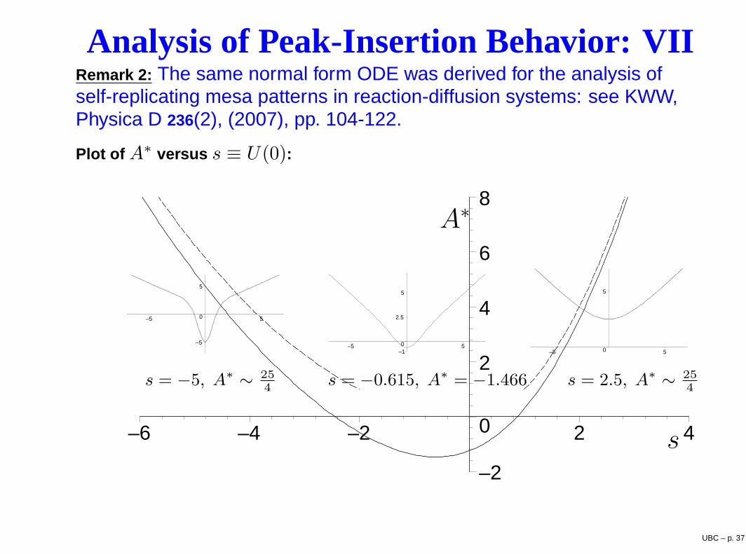
Analysis of Peak-Insertion Behavior: VIIRemark 2: The same normal form ODE was derived for the analysis ofself-replicating mesa patterns in reaction-diffusion systems: see KWW,Physica D 236(2), (2007), pp. 104-122.

Plot of A∗ versus s ≡ U(0):

–2

0

2

4

6

8

–6 –4 –2 2 4

–5

0

5

–5 5

s = −5, A∗

∼25

4

–10

2.5

5

–5 5

s = −0.615, A∗

= −1.466

0

5

–5 5

s = 2.5, A∗

∼25

4

A∗

s

UBC – p. 37

Finite-Dimensional Dynamics: D = O(1): I

On the basic cell, |x| ≤ l, one can construct a quasi-equilibrium one-spikesolution centered at x = x0, where x0 = x0(ε

2t) moves slowly in time.

Main Result: Provided that no peak-insertion effects occur, then for ε→ 0the dynamics on the slow time-scale σ = ε2t is characterized by

A ∼ ε−1w (y) /√

v0 , y = ε−1(x− x0(σ)) ,

dx0dσ

∼ 3

8αF(x0) , F(x0) ≡

[

a0x(x+0 ) + a0x(x

−

0 )]

.

Here a0(x) is the solution to the multi-point BVP

D [f(a0)a0x]x = a0 − γ , 0 < |x| < l ; a0x(±l) = 0 , a0(0) = α ,

where f(a0) ≡ a−20 (3α− 2a0).

Remark 1: The derivation of this is delicate in that one must resolve acorner layer or knee region for V that allows for matching between theinner and outer approximations for V .

UBC – p. 38

Finite-Dimensional Dynamics D = O(1): IIFrom an integration of the BVP for a0, one gets explicit dynamics:

dx0dσ

=3

8

(

2

D

)

[

√

G(α;µr)−√

G(α;µl)]

,

where µr ≡ a0(l) and µl ≡ a0(−l) are determined implicitly by√

2

D(l − x0) = χ(µr) ,

√

2

D(l + x0) = χ(µl) .

Qualitative I: The dynamics is repulsive: If x0(0) > 0, then x0 → 0 ast→ ∞. By using reflection through the Neumann B.C., two adjacenthot-spots will repel.

Qualitative II: Since the hot-spot dynamics is repulsive, then dynamicpeak-insertion events due to large inter-hot-spot separations are unlikely.

Remark: Peak insertion events in the presence of mutually attractinglocalized pulses, leads to spatial temporal chaos in a Keller-Segel modelwith logistic growth in 1-D (Painter and Hillen, Physica D 2011).

UBC – p. 39

The Effect of Police: 3-Component SystemsIn 1-D, an RD system incorporating police is U = U(x, t):

At = ε2∆A−A+ PA+ α , x ∈ Ω ,

Pt = D∇ ·(

∇P − 2P

A∇A

)

− PA+ γ − α− f , x ∈ Ω ,

τuUt = D∇ ·(

∇U − qU

A∇A

)

, x ∈ Ω ,

with ∂n(A,P, U) = 0 on ∂Ω. Police are conserved; U0 =∫

ΩU dx > 0 for all t.

Police Model I: f = U (simple interaction ) L. Ricketson (UCLA).

Police Model II: f = UP (standard “predator-prey” type interaction )

Remark: The police drift velocity is V = ddx ln(Aq).

If q = 2, police drift exhibits mimicry (L. Ricketson, UCLA) Referred toas “Cops on the Dots” (Jones, Brantingham, L. Chayes, M3As, 2011).Can be derived from an agent-based model.

If q > 2, police focus more on attractive sites than do criminals.

If 0 < q < 2, the police are less focused, and more “diffusive”.UBC – p. 40

The Effect of Police: QualitativeQuestion I: Optimal Police Strategy: For a given U0 find the optimal q(parameter in police drift velocity) that minimizes the NLEP stabilitythreshold of D with D = D0/ε

2. In this way, we maximize over q thedistance between stable localized hot-spots.

Investigate this question for both Police models I and II.

Is the optimal strategy the same for both models?

Question II: For τu sufficiently large on the regime D = O(ε−2),corresponding to police diffusivity D/τu, can a two-hot spot solutionundergo a Hopf bifurcation leading to asynchronous temporal oscillationsin the hot-spot amplitudes?

If τu > 1, then police ‘diffuse” more slowly than do criminals.

Typically, only synchronous oscillatory instabilities of the spikeamplitudes occur in RD systems (GM, Gray-Scott, etc..)

Question III: Open: For D = O(1) can police prevent or limit the nucleationof new hot-spots of criminal activity arising from peak-insertion?

UBC – p. 41

Police Model I: Simple-Interaction ModelPrincipal Result (Equilibrium) : On the basic cell |x| > l, and with q > 1, theleading order asymptotics for A, P , and U , in the hot-spot region nearx = 0 is

A ∼ 1

ε√v0w (x/ε) , P ∼ [w (x/ε)]

2, U ∼ U0

εb[w (x/ε)]

q.

Here b ≡∫

wq dy, and w = w(y) =√2sech (y) is the homoclinic of

w′′−w+w3 = 0. The amplitude of the hot-spot is determined by v0, where

1√v0

∫

w3 dy = 2l(γ − α)− U0 .

Remark I: A hot-spot solution ceases to exist if the total number of policesatisfies

U0 ≥ U0c ≡ 2l(γ − α)

Remark II: For U0 < U0c, for a K-spot equilibrium on a domain of length S,let l = S/(2K) and replace U0 → U0/K. Then, use a glueing technique toconstruct the multi-pulse pattern.

UBC – p. 42

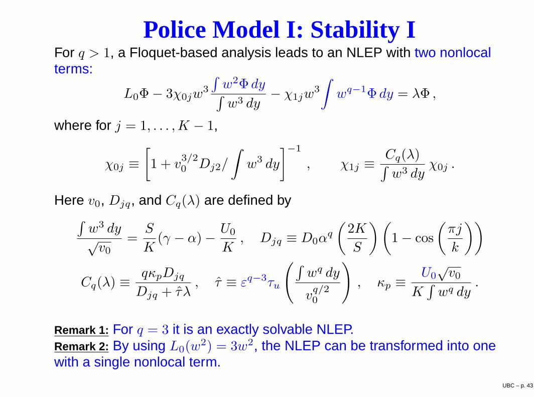
Police Model I: Stability IFor q > 1, a Floquet-based analysis leads to an NLEP with two nonlocalterms:

L0Φ− 3χ0jw3

∫

w2Φ dy∫

w3 dy− χ1jw

3

∫

wq−1Φ dy = λΦ ,

where for j = 1, . . . ,K − 1,

χ0j ≡[

1 + v3/20 Dj2/

∫

w3 dy

]−1

, χ1j ≡Cq(λ)∫

w3 dyχ0j .

Here v0, Djq, and Cq(λ) are defined by∫

w3 dy√v0

=S

K(γ − α)− U0

K, Djq ≡ D0α

q

(

2K

S

)(

1− cos

(

πj

k

))

Cq(λ) ≡qκpDjq

Djq + τλ, τ ≡ εq−3τu

(

∫

wq dy

vq/20

)

, κp ≡ U0√v0

K∫

wq dy.

Remark 1: For q = 3 it is an exactly solvable NLEP.Remark 2: By using L0(w

2) = 3w2, the NLEP can be transformed into onewith a single nonlocal term.

UBC – p. 43

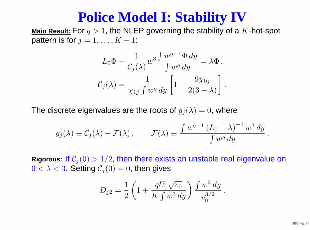
Police Model I: Stability IVMain Result: For q > 1, the NLEP governing the stability of a K-hot-spotpattern is for j = 1, . . . ,K − 1:

L0Φ− 1

Cj(λ)w3

∫

wq−1Φ dy∫

wq dy= λΦ ,

Cj(λ) =1

χ1j

∫

wq dy

[

1− 9χ0j

2(3− λ)

]

.

The discrete eigenvalues are the roots of gj(λ) = 0, where

gj(λ) ≡ Cj(λ)−F(λ) , F(λ) ≡∫

wq−1 (L0 − λ)−1w3 dy

∫

wq dy.

Rigorous: If Cj(0) > 1/2, then there exists an unstable real eigenvalue on0 < λ < 3. Setting Cj(0) = 0, then gives

Dj2 =1

2

(

1 +qU0

√v0

K∫

w3 dy

)∫

w3 dy

v3/20

.

UBC – p. 44

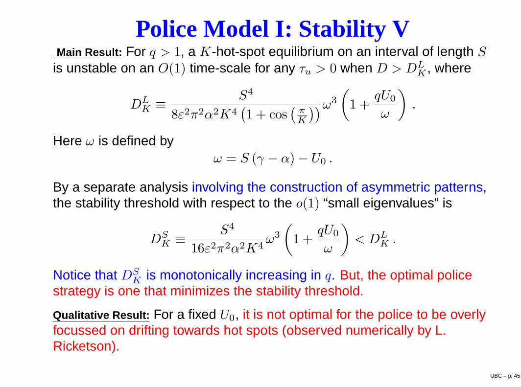
Police Model I: Stability VMain Result: For q > 1, a K-hot-spot equilibrium on an interval of length S

is unstable on an O(1) time-scale for any τu > 0 when D > DLK , where

DLK ≡ S4

8ε2π2α2K4(

1 + cos(

πK

))ω3

(

1 +qU0

ω

)

.

Here ω is defined byω = S (γ − α)− U0 .

By a separate analysis involving the construction of asymmetric patterns,the stability threshold with respect to the o(1) “small eigenvalues” is

DSK ≡ S4

16ε2π2α2K4ω3

(

1 +qU0

ω

)

< DLK .

Notice that DSK is monotonically increasing in q. But, the optimal police

strategy is one that minimizes the stability threshold.

Qualitative Result: For a fixed U0, it is not optimal for the police to be overlyfocussed on drifting towards hot spots (observed numerically by L.Ricketson).

UBC – p. 45

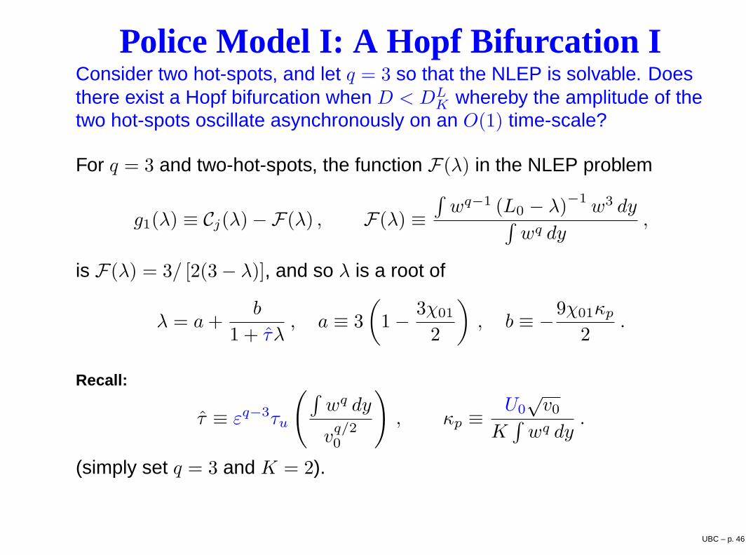
Police Model I: A Hopf Bifurcation IConsider two hot-spots, and let q = 3 so that the NLEP is solvable. Doesthere exist a Hopf bifurcation when D < DL

K whereby the amplitude of thetwo hot-spots oscillate asynchronously on an O(1) time-scale?

For q = 3 and two-hot-spots, the function F(λ) in the NLEP problem

g1(λ) ≡ Cj(λ)−F(λ) , F(λ) ≡∫

wq−1 (L0 − λ)−1w3 dy

∫

wq dy,

is F(λ) = 3/ [2(3− λ)], and so λ is a root of

λ = a+b

1 + τλ, a ≡ 3

(

1− 3χ01

2

)

, b ≡ −9χ01κp2

.

Recall:

τ ≡ εq−3τu

(

∫

wq dy

vq/20

)

, κp ≡ U0√v0

K∫

wq dy.

(simply set q = 3 and K = 2).

UBC – p. 46

Police Model I: A Hopf Bifurcation II

Main Result: For q = 3 and K = 2, there exists a Hopf Bifurcation atτu = τuH with λ = ±iλI , when 0 < DH

K < D < DLK . We have,

τuH =v3/20 D13

a∫

w3 dy, λI =

√

−a(a+ b) .

There is an explicit formula for DHK . No Hopf bif. if D < DH

K .

Qualitative: If τu > τuH on 0 < DHK < D < DL

K , we predict asychronousoscillatory instability of the two spots. Numerically, the bifurcation lookssupercritical. If D < DH

K , then we have stability for all τu.

Interpretation: There is an intermediate range of police diffusivity (slowerthan criminals) for which the two hot-spots exhibit asynchronousoscillations. Maximum criminal activity is displaced periodically in timefrom one hot-spot to its neighbour.

Remark: Similar behavior for is expected for q 6= 3, but is more difficult toanalyze. (no explicit analytical formulas available).

UBC – p. 47

Police Model II: Predator-Prey InteractionPrincipal Result (Equilibrium) : On the basic cell |x| > l, and with q > 1, theleading order asymptotics for A, P , and U , in the hot-spot region nearx = 0 is

A ∼ 1

ε√v0w (x/ε) , P ∼ [w (x/ε)]

2, U ∼ U0

εb[w (x/ε)]

q.

Here b ≡∫

wq dy, and w = w(y) =√2sech (y) is the homoclinic of

w′′−w+w3 = 0. The amplitude of the hot-spot is determined by v0, where

1√v0

∫

w3 dy = 2l(γ − α)− U0

∫

w2+q dy∫

wq dy,

∫

w2+q dy∫

wq dy=

2q

q + 1.

Remark I: A hot-spot solution ceases to exist if

U0 ≥ U0c ≡ (q + 1)l(γ − α)/q.

Remark II: For U0 < U0c, for a K-spot equilibrium on a domain of length S,let l = S/(2K) and replace U0 → U0/K. Then, use a glueing technique toconstruct the multi-pulse pattern.

UBC – p. 48

Police Model II: Stability ILet q > 1, and U0 < U0c so that a K-hot-spot equilibrium exists. Then:

Small Eigenvalue Threshold: Asymmetric hot-spot equilibria bifurcate fromthe symmetric K-hot-spot branch at the threshold

DSK ≡ ω3S

16ε2π2α2K4

(

1 +2q2U0

(q + 1)ω

)

, ω ≡ S(γ − α)− 2U0q

q + 1> 0 .

(Note that the amplitude of the hot-spot is proportional to ω.)

NLEP Analysis: The NLEP now involves 3 separate nonlocal terms. Whenτu ≪ O(εq−3), the stability threshold for this NLEP is

DLK = DS

K

(

2

1 + cos (π/K)

)

> DSK .

By simple calculus we study DSK as a function of q for U0 fixed with

U0 < U0c. Optimal strategy is to minimize the threshold.

UBC – p. 49

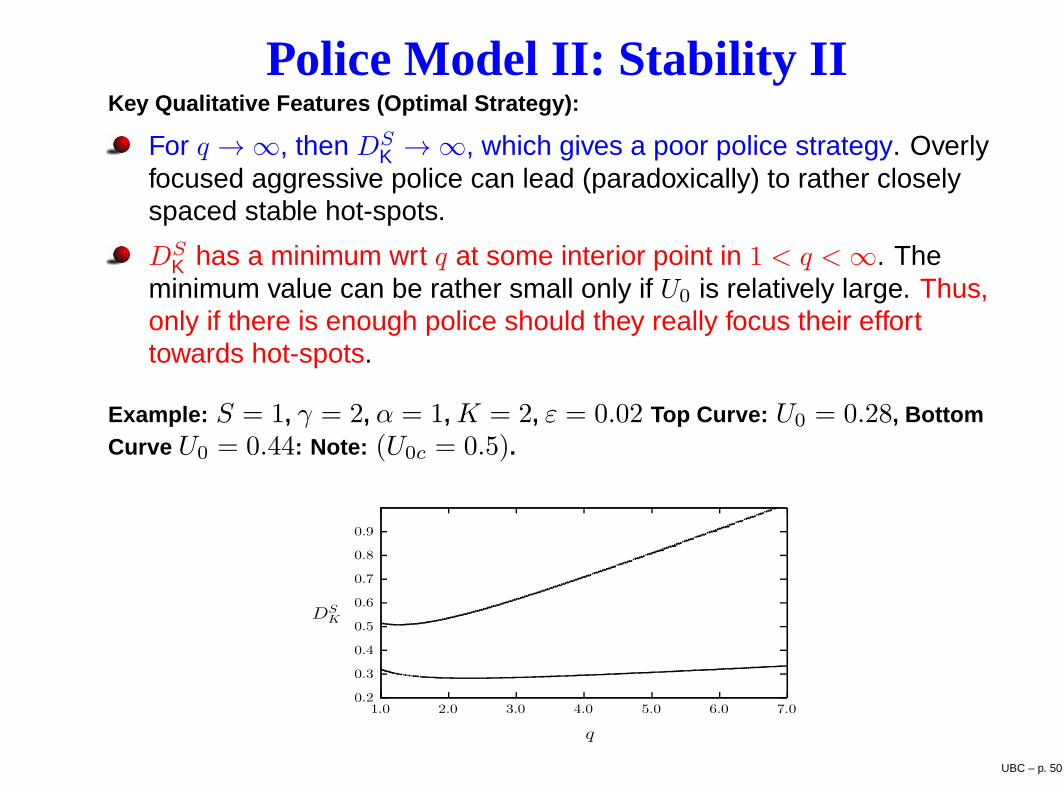
Police Model II: Stability IIKey Qualitative Features (Optimal Strategy):

For q → ∞, then DSK → ∞, which gives a poor police strategy. Overly

focused aggressive police can lead (paradoxically) to rather closelyspaced stable hot-spots.

DSK has a minimum wrt q at some interior point in 1 < q <∞. The

minimum value can be rather small only if U0 is relatively large. Thus,only if there is enough police should they really focus their efforttowards hot-spots.

Example: S = 1, γ = 2, α = 1, K = 2, ε = 0.02 Top Curve: U0 = 0.28, BottomCurve U0 = 0.44: Note: (U0c = 0.5).

0.2

0.3

0.4

0.5

0.6

0.7

0.8

0.9

1.0 2.0 3.0 4.0 5.0 6.0 7.0

DSK

q

UBC – p. 50

Further DirectionsFor the basic urban crime model in 2-D with D = O(1):

Investigate effect of spatial heterogeneity of γ, α.Derive the scalar nonlinear elliptic PDE, associated with asaddle-node point, governing peak insertion.Dynamics in 1-D and 2-D: Derive ODE’s for the locations of centers of acollection of hot-spots (repulsive interactions?).Are dynamic peak-insertion events for a collection of hot-spotspossible? If hot-spots become too closely spaced, we anticipateannihilation. Can annihilation and creation events lead tospatial-temporal chaos?

Analyze other models of the effect of police, incorporating dynamicdeterrence, i.e. A. Pilcher, EJAM (2010).

References:T. Kolokolnikov, M.J. Ward, J. Wei, The Stability of Steady-State Hot-SpotPatterns for a Reaction-Diffusion Model of Urban Crime, to appearDCDS-B, (2012), (34 pages).

T. Kolokolnikov, S. Tse, M.J. Ward, J. Wei, Urban Crime, Hot-SpotPatterns, and the Effect of Police: a Three-Component Reaction-DiffusionModel, in preparation, (2012). UBC – p. 51