the square root law of steganographic capacity
TRANSCRIPT
The Square Root Law of
Steganographic Capacity
Andrew [email protected]
Oxford University Computing Laboratory
ACM Multimedia & Security Workshop
Oxford, 22 September 2008
Tomáš Pevný[email protected]
Jessica [email protected]
Jan Kodovský[email protected]
Binghamton University SUNY

BackgroundThe more information you hide, the greater your risk of discovery.
The steganographic capacity question is:
Given a particular limit on risk, how much can you hide?
A key part of this question, though rarely asked, is:
How does the secure capacity depend on the size of the cover?
Ross Anderson in the 1st Information Hiding Workshop (1996):
“…the more covertext we give the warden, the better he
will be able to estimate its statistics, and so the smaller
the rate at which Alice will be able to tweak bits safely.
The rate might even tend to zero...”
The Square Root Law of
Steganographic Capacity
Outline
• Background
• Steganographic capacity theorems
• Experimental design
• Results
• Conclusions
Capacity theoremsRandomly modulated codes (Wang & Moulin, 2008)
Hides information which is perfectly undetectable, at a linear rate, but
requires the embedder to have complete knowledge of their cover source.
Batch steganographic capacity theorem (Ker, 2007)
Applies to multiple independent covers. Under certain assumptions, total
capacity is asymptotically proportional to square root of number of covers.
Batch steganographic strategies (Ker, 2008)
Under certain conditions, KL divergence is locally quadratic; implies that total
capacity is asymptotically proportional to square root of number of covers.
Square root law for Markov chains (Filler, Ker, & Fridrich, 2009)
When cover can be modelled as a Markov chain, and embedding as
independent state change, if embedding is not perfect then the max change
rate is asymptotically inversely proportional to square root of cover size.
AimInvestigate empirically the relationship between cover size, payload size,
and detectability of payload.
Related work can be found in:
� Ker, IHW 2004 � Böhme, IHW 2005 � Böhme & Ker, SPIE EI 2006
The idea is to fix the:
then produce cover images of different sizes from the parent set, and
investigate detectability.
But it is difficult to make image sets of different sizes which do not also
have different characteristics: noise, density, etc.
The best we can do is crop down large images to smaller ones, choosing the
crop region to preserve local variance as much as possible.
• parent cover set,
• embedding method,
• detector,
• detectability metric,

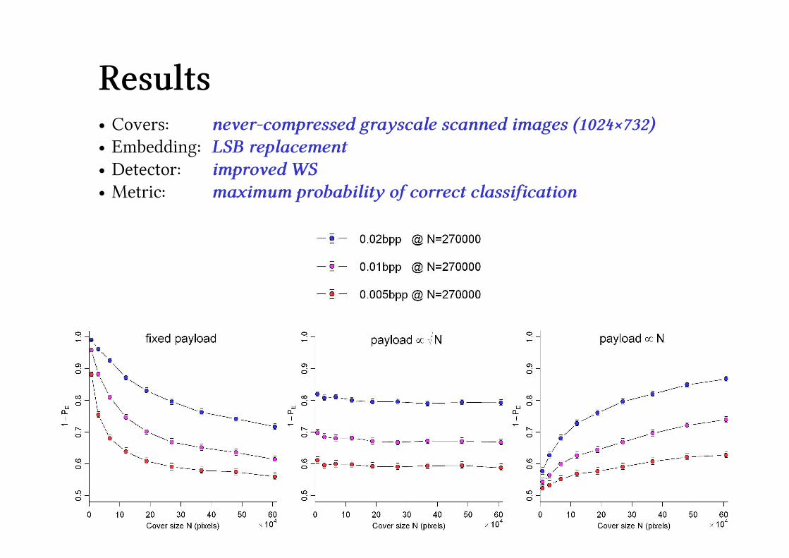
Results• Covers: never-compressed grayscale scanned images (1024×732)
• Embedding: LSB replacement
• Detector: improved WS
• Metric: maximum probability of correct classificationbootstrapped approx. 90% confidence intervals
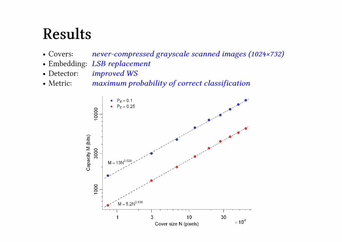
Results• Covers: never-compressed grayscale scanned images (1024×732)
• Embedding: LSB replacement
• Detector: improved WS
• Metric: maximum probability of correct classification
Results• Covers: never-compressed grayscale scanned images (1024×732)
• Embedding: LSB replacement
• Detector: improved WS
• Metric: maximum probability of correct classification
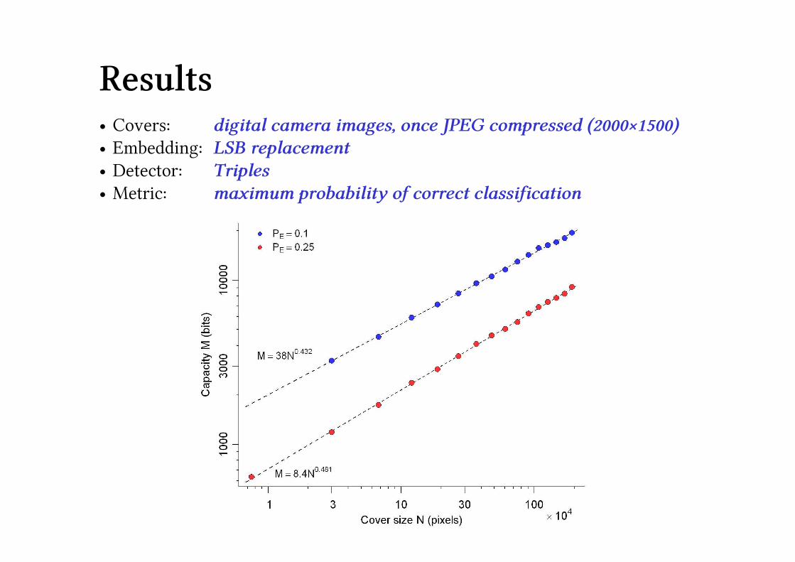
Results• Covers: digital camera images, once JPEG compressed (2000×1500)
• Embedding: LSB replacement
• Detector: Triples
• Metric: maximum probability of correct classification

Results• Covers: never-compressed grayscale scanned images (1024×732)
• Embedding: LSB matching (±1)
• Detector: adjacency HCF COM
• Metric: maximum probability of correct classification
JPEG embeddingTwo additional challenges:
1. How to measure size?
We count nonzero quantized DCT coefficients.
2. How to crop images?
We crop to an 8×8 grid, choosing region:
• to select desired number of nonzero coefficients,
• while preserving the ratio of nonzero coefficients to all coefficients as much
as possible.
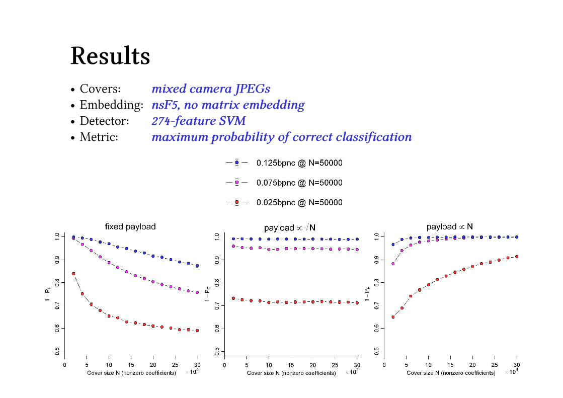
Results• Covers: mixed camera JPEGs
• Embedding: nsF5, no matrix embedding
• Detector: 274-feature SVM
• Metric: maximum probability of correct classification

Results• Covers: mixed camera JPEGs
• Embedding: nsF5, no matrix embedding
• Detector: 274-feature SVM
• Metric: maximum probability of correct classification
Conclusions• Exploring a range of cover image types, embedding methods, detectors, and
detectability metrics, we observed close accordance with a square root law.
Of course, this is no proof of a square root law in general. The full law
will be a suite of theorems proving that it holds under a variety of
conditions.
• Two important limitations of the law:
– It does not apply when perfect steganography is available.
– It properly applies to the number of embedding changes, not payload.
It turns out that payload capacity is of order given best
adaptive source coding.
• Has many consequences for the practice of steganography and steganalysis:
– Must take care when designing steganographic file systems.
– “Bits per pixel”, “bits per nonzero coefficient” are the wrong measures…