the split delivery vehicle routing problembgolden/recent_presentation_pdfs_links... · 2...
TRANSCRIPT
1
The Split Delivery Vehicle Routing Problem
by
Si Chen, University of Maryland
Bruce Golden, University of Maryland
Edward Wasil, American University
Graph Theory, Algorithms, and Applications
Erice, Italy, September 11, 2008

2
Introduction
� The split delivery vehicle routing problem (SDVRP)
� A relaxation of traditional VRP
� A customer’s demand can be split between two or more vehicles
� DT heuristic by Dror and Trudeau
� SplitTabu heuristic by Archetti et al.
� The potential exists to save vehicles and thus reduce distance traveled
3
Applications
� Livestock feed distribution (via trucks) to pens at a ranch
� Routing helicopters for crew exchange at off-shore locations
� Distributing bundles of newspapers in Korea
� Containerized sanitation pick-up/commercial collection
4
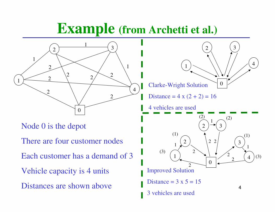
Example (from Archetti et al.)
2 3
1
4
0
1
1
1
22
2
22
2 2
0
1
2 3
4
Node 0 is the depot
There are four customer nodes
Each customer has a demand of 3
Vehicle capacity is 4 units
Distances are shown above
Clarke-Wright Solution
Distance = 4 x (2 + 2) = 16
4 vehicles are used
Improved Solution
Distance = 3 x 5 = 15
3 vehicles are used
(2) (2)
01
2 3
4
2 31
1
1
2
2
2 2
22
(3)
(1) (1)
(3)

5
DT Heuristic
� A k-split interchange splits the demand of customer i
among k routes provided that
� capacity constraints are obeyed, and
� total distance is reduced
vehicle capacity = 3
0
12
3
(2)(2)
(2)
1 2
0
(2) (1)
2
0
3
(1)
(2)
Example of a 2-split interchange
plus

6
DT Heuristic
� Route addition serves as an inverse operation to a k-split
interchange
� Add a route to eliminate a split delivery
� Do so if it reduces total distance
Example of a route addition
0
12
3
(2)(2)
(2)
0
1
2
3
(2)
(1)
(2)2
(1)
7
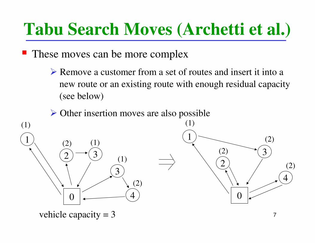
Tabu Search Moves (Archetti et al.)
� These moves can be more complex
� Remove a customer from a set of routes and insert it into a
new route or an existing route with enough residual capacity
(see below)
� Other insertion moves are also possible
0
1
2
3
(1)
(2)
(2)
0
1
2
3
(1)
(2)
(1)3
(1)
vehicle capacity = 3
4
(2)4
(2)

8
Computational Results for the
DT Heuristic� Based on a Euclidean problem with 75 nodes
� Vehicle capacity is 160 units
� Six demand scenarios
a) [0.01 – 0.1] d) [0.1 – 0.9]
b) [0.1 – 0.3] e) [0.3 – 0.7]
c) [0.1 – 0.5] f) [0.7 – 0.9]
� Demand i in scenario [α – β ] is generated randomly from a
uniform distribution on the interval [ 160 α , 160 β ]
� There are 30 instances per scenario
9
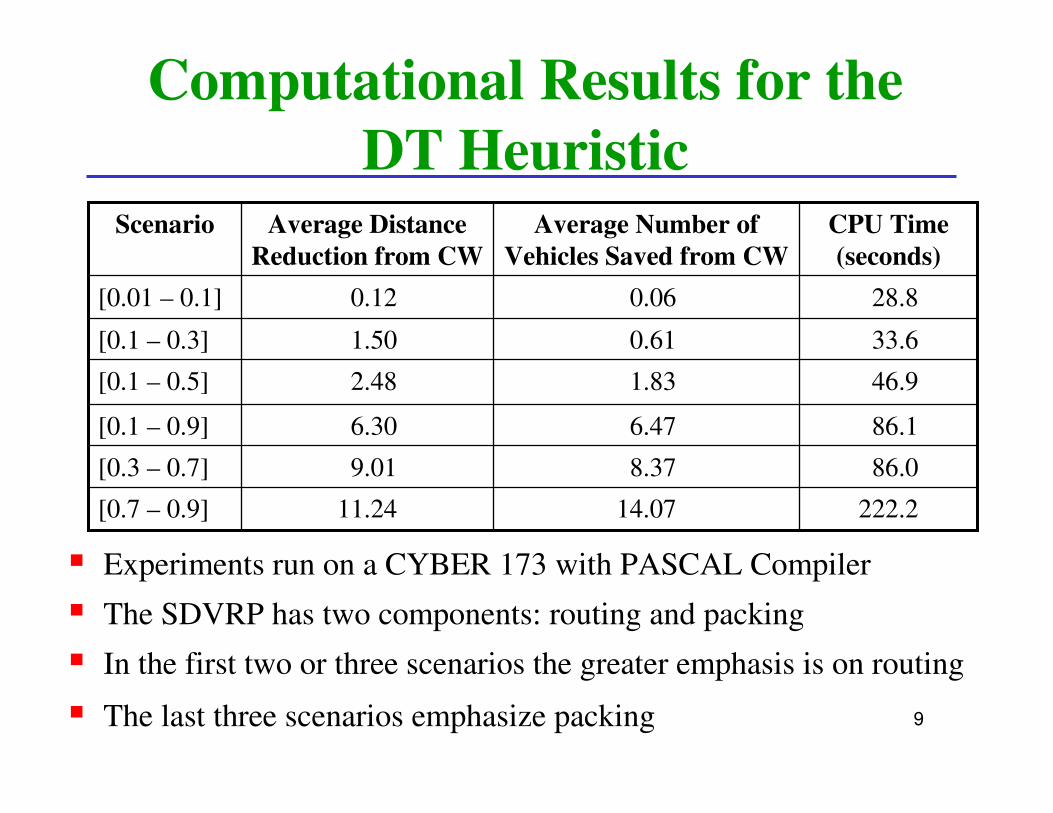
Computational Results for the
DT Heuristic
� Experiments run on a CYBER 173 with PASCAL Compiler
� The SDVRP has two components: routing and packing
� In the first two or three scenarios the greater emphasis is on routing
� The last three scenarios emphasize packing
222.214.0711.24[0.7 – 0.9]
86.08.379.01[0.3 – 0.7]
86.16.476.30[0.1 – 0.9]
46.91.832.48[0.1 – 0.5]
33.60.611.50[0.1 – 0.3]
28.80.060.12[0.01 – 0.1]
CPU Time
(seconds)
Average Number of
Vehicles Saved from CW
Average Distance
Reduction from CW
Scenario

10
A New MIP Approach
� Start with an initial solution (e.g., the CW solution)
� For each route in this solution, consider its one or two
endpoints
� For each endpoint, we consider its l-closest endpoints to be
its “neighbors” (l is a parameter)
� Each endpoint is allowed to reallocate its demand among its
neighbors
� After this reallocation process, there are three possibilities
for each endpoint (we assume symmetry here)
� No change is made

11
A New MIP Approach� The endpoint i is removed from its current route(s)
and all of its demand is moved to another route or routes
(see below for simple example)
i - 1
i
0
j
i - 1
i
0
j
Savings = ( l i-1, i + l i, 0 – l i-1, 0 )
– ( l 0, i + l i, j – l 0, j )

12
A New MIP Approach� Part of the demand of endpoint i is moved to another route
or routes
i - 1
i
0
j
Savings = – ( l 0, i + l i, j – l 0, j )
i - 1
i
0
i
j
13
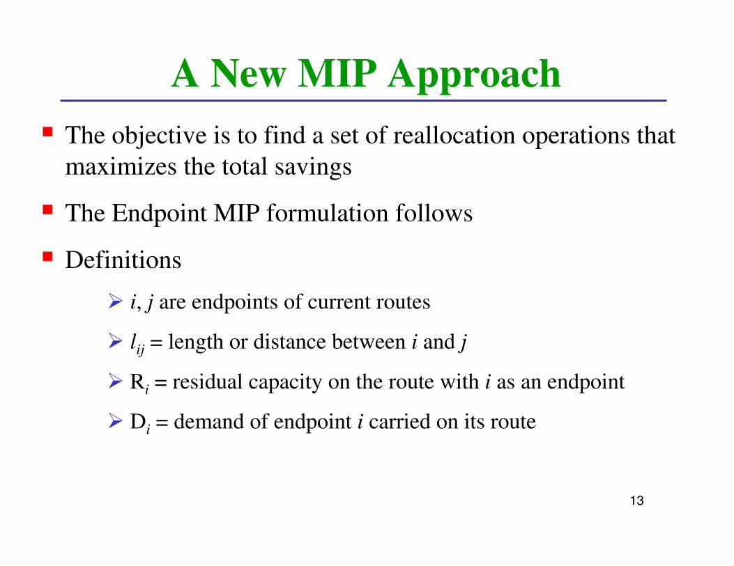
A New MIP Approach
� The objective is to find a set of reallocation operations that
maximizes the total savings
� The Endpoint MIP formulation follows
� Definitions
� i, j are endpoints of current routes
� lij = length or distance between i and j
� Ri = residual capacity on the route with i as an endpoint
� Di = demand of endpoint i carried on its route
14
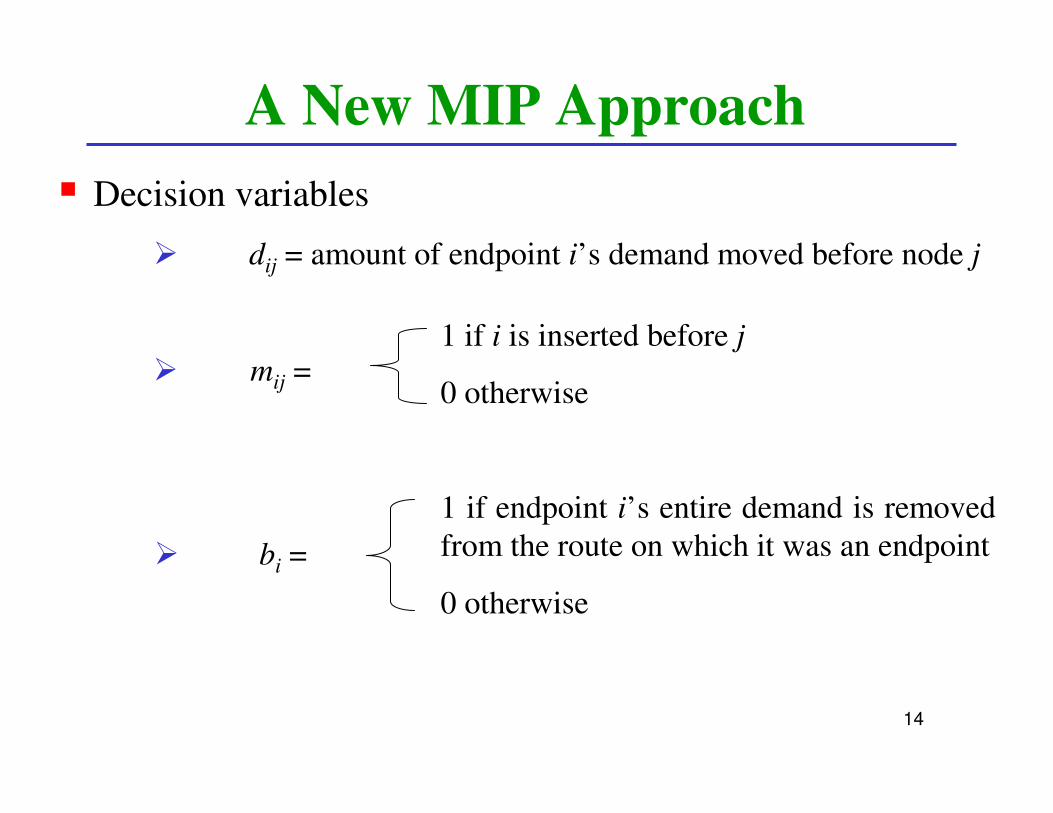
A New MIP Approach
� Decision variables
� dij = amount of endpoint i’s demand moved before node j
1 if i is inserted before j
0 otherwise
1 if endpoint i’s entire demand is removed
from the route on which it was an endpoint
0 otherwise
� mij =
� bi =

15
Endpoint MIP Constraints
� The amount added to a route minus the amount taken away < residual capacity
� The amount diverted from an endpoint on a route < its demand on that route
� If an endpoint is removed from a route, all of its demand must be diverted to other routes
� If dij > 0 => mij = 1
� If an endpoint is removed from a route, no other endpoint can be inserted before it
� dij > 0, bi & mij 0 {0, 1}
16
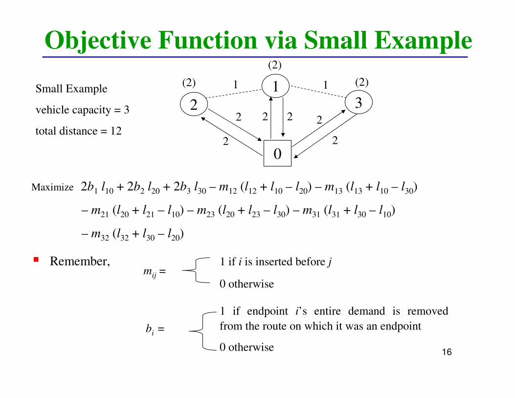
Objective Function via Small Example
� Remember, 1 if i is inserted before j
0 otherwise
1 if endpoint i’s entire demand is removed
from the route on which it was an endpoint
0 otherwise
mij =
bi =
2
13
Small Example
vehicle capacity = 3
total distance = 12
0
Maximize 2b1 l10 + 2b2 l20 + 2b3 l30 – m12 (l12 + l10 – l20) – m13 (l13 + l10 – l30)
– m21 (l20 + l21 – l10) – m23 (l20 + l23 – l30) – m31 (l31 + l30 – l10)
– m32 (l32 + l30 – l20)
1 1(2) (2)
(2)
2
2
2 2 2
2
17
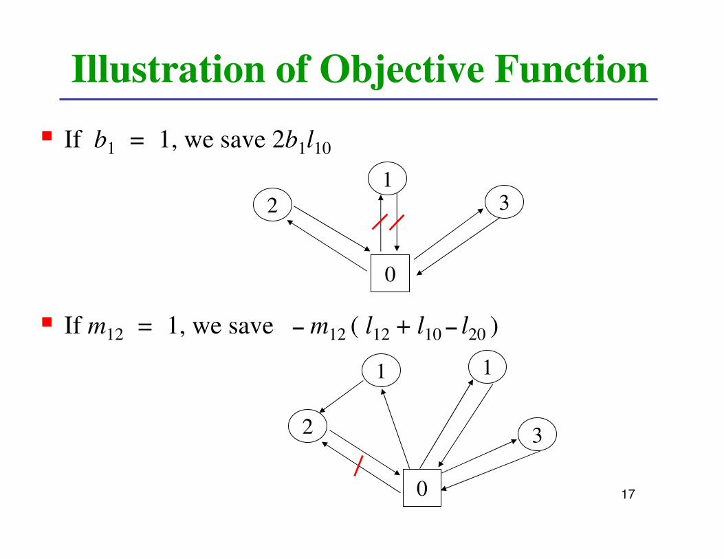
Illustration of Objective Function
� If b1 = 1, we save 2b1l10
� If m12 = 1, we save – m12 ( l12 + l10 – l20 )
2
13
0
2
1 1
3
0
18
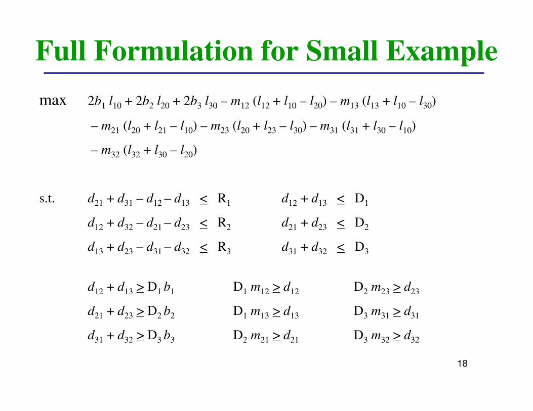
Full Formulation for Small Example
max 2b1 l10 + 2b2 l20 + 2b3 l30 – m12 (l12 + l10 – l20) – m13 (l13 + l10 – l30)
– m21 (l20 + l21 – l10) – m23 (l20 + l23 – l30) – m31 (l31 + l30 – l10)
– m32 (l32 + l30 – l20)
s.t. d21 + d31 – d12 – d13 < R1 d12 + d13 < D1
d12 + d32 – d21 – d23 < R2 d21 + d23 < D2
d13 + d23 – d31 – d32 < R3 d31 + d32 < D3
d12 + d13 > D1 b1 D1 m12 > d12 D2 m23 > d23
d21 + d23 > D2 b2 D1 m13 > d13 D3 m31 > d31
d31 + d32 > D3 b3 D2 m21 > d21 D3 m32 > d32

19
� Continuation of constraints
1 – b1 > m21 + m31
1 – b2 > m32 + m12
1 – b3 > m23 + m13
dij > 0
bi & mij 0 {0, 1}
� MIP solution
total distance = 102
1 1
3
0
Full Formulation for Small Example
(2)
2
1
(1) (1)
(2)1
2 2
2
20
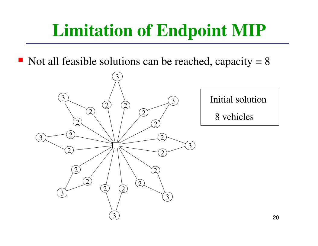
Limitation of Endpoint MIP
� Not all feasible solutions can be reached, capacity = 8
3
33
3
3
3
3
22
2
2
2
22
2
2
2
2
2
2
2
2
2
3
Initial solution
8 vehicles
21
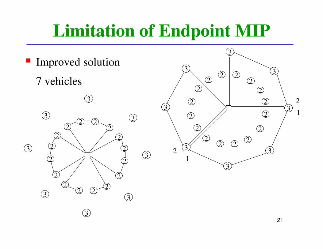
Limitation of Endpoint MIP
� Improved solution
7 vehicles
3
33
3
3
3
3
22
2
2
2
22
2
2
2
2
2
2
2
2
2
3
3
33
3
3
3
3
22
2
2
2
22
2
2
2
2
2
2
2
2
2
3
21
1
2
22
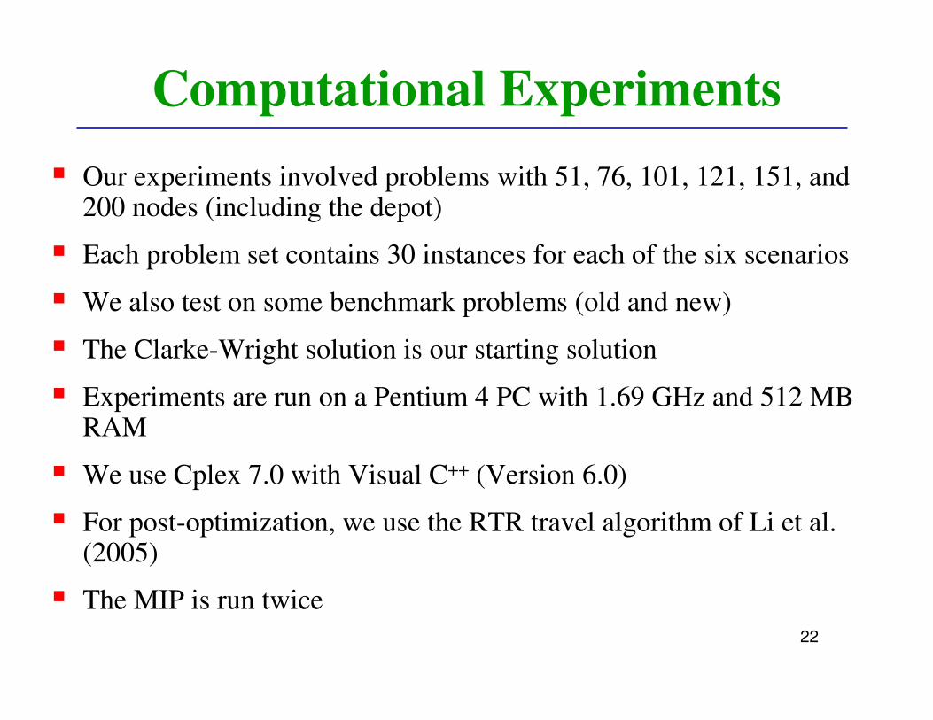
� Our experiments involved problems with 51, 76, 101, 121, 151, and 200 nodes (including the depot)
� Each problem set contains 30 instances for each of the six scenarios
� We also test on some benchmark problems (old and new)
� The Clarke-Wright solution is our starting solution
� Experiments are run on a Pentium 4 PC with 1.69 GHz and 512 MB RAM
� We use Cplex 7.0 with Visual C++ (Version 6.0)
� For post-optimization, we use the RTR travel algorithm of Li et al. (2005)
� The MIP is run twice
Computational Experiments

23
� We compare the MIP approach with the best tabu search variant from Archetti et al. (SplitTabu-DT)
� Archetti et al. use a Pentium 4 PC with 0.8 GHz and 256 MB RAM
� The comparison is approximate since SplitTabu-DT was only tested on one instance for each scenario in each problem set
� In contrast, we run 30 instances for each scenario in each problem set
Comparison of the Two Heuristics

24
Computational Comparison
216,521
149,690
146,992
100,867
76,140
46,376
Tabu
5.04106.0135.4205,600206,841240,196[0.7 - 0.9]
5.8948.647.9140,867143,482164,461[0.3 - 0.7]
4.1960.855.4140,833145,124156,833[0.1 - 0.9]
6.4328.214.794,38599,117105,456[0.1 - 0.5]
4.9721.83.472,35676,12978,776[0.1 - 0.3]
1.414.81.945,72149,75549,955[0.01 – 0.1]
%
BetterTimeTimeMIP + PPMIPCWScenario
� 51 nodes, capacity = 160
25
Computational Comparison
318,064
216,051
212,443
144,362
109,532
60,524
Tabu
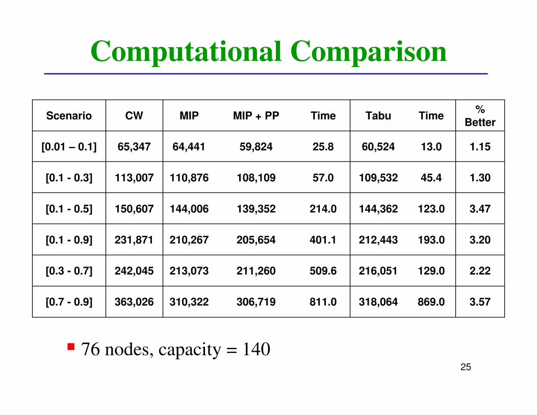
3.57869.0811.0306,719310,322363,026[0.7 - 0.9]
2.22129.0509.6211,260213,073242,045[0.3 - 0.7]
3.20193.0401.1205,654210,267231,871[0.1 - 0.9]
3.47123.0214.0139,352144,006150,607[0.1 - 0.5]
1.3045.457.0108,109110,876113,007[0.1 - 0.3]
1.1513.025.859,82464,44165,347[0.01 – 0.1]
%
BetterTimeTimeMIP + PPMIPCWScenario
� 76 nodes, capacity = 140

26
Computational Comparison
486,779
303,802
310,153
202,999
146,201
64,874
Tabu
1.821004.41024.3477,9124,800,264577,014[0.7 - 0.9]
-3.18777.8716.5313,455317,790381,021[0.3 - 0.7]
-1.96259.6251.2316,221322,146366,489[0.1 - 0.9]
2.79292.8287.6197,333207,735215,267[0.1 - 0.5]
3.26146.0126.5141,432148,479151,851[0.1 - 0.3]
-0.4257.853.965,14367,24069,755[0.01 – 0.1]
% BetterTimeTimeMIP + PPMIPCWScenario
� 101 nodes, capacity = 200

27
Computational Comparison
1,030,408
663,955
658,397
420,612
291,871
108,470
Tabu
13.221825.6725.4894,178899,8131,223,830[0.7 - 0.9]
7.77658.6605.4612,395625,696756,257[0.3 - 0.7]
7.67877.8722.8607,913632,431751,617[0.1 - 0.9]
12.34268.0220.7368,705400,437425,153[0.1 - 0.5]
11.99142.6136.4256,889285,080291,471[0.1 - 0.3]
9.1842.436.498,516100,353102,583[0.01 – 0.1]
% BetterTimeTimeMIP + PPMIPCWScenario
� 121 nodes, capacity = 200

28
Computational Comparison
619,636
403,970
390,972
263,271
191,825
89,095
Tabu
3.9710,223.010,038.8595,034598,738735,924[0.7 - 0.9]
0.693,008.03,028.3401,173413,049474,211[0.3 - 0.7]
-0.912,278.02,220.0394,537410,578465,426[0.1 - 0.9]
3.79739.2630.5253,292266,581281,996[0.1 - 0.5]
3.82393.2308.0184,495194,325199,700[0.1 - 0.3]
1.77172.8107.887,51594,42096,249[0.01 – 0.1]
%
BetterTimeTimeMIP + PPMIPCWScenario
� 151 nodes, capacity = 200

29
Computational Comparison
794,463
510,284
485,383
328,447
238,415
105,627
Tabu
9.2821,849.012,542.3720,703734,454960,678[0.7 - 0.9]
0.293,565.63,035.7508,807524,037615,268[0.3 - 0.7]
-4.963,297.23,038.1509,460521,442592,915[0.1 - 0.9]
2.492,668.01,775.7320,256340,604359,392[0.1 - 0.5]
5.26754.8618.5225,865242,205250,659[0.1 - 0.3]
1.52525.8413.4104,019114,245114,303[0.01 – 0.1]
%
BetterTimeTimeMIP + PPMIPCWScenario
� 200 nodes, capacity = 200
30
Some Observations From Statistics
� If Tabu and MIP + PP are equally good with respect to quality of solution, then Tabu would beat the median MIP + PP result about half the time
� Using a binomial distribution with n = 36 and p = ½, we can test the null hypothesis that they are equally good
� Using a significance level of 0.01, the Tabu results should beat the median MIP + PP results in at least 10 out of 36 cases
� Since Tabu wins in only 5 out of 36 cases, the null hypothesis is clearly rejected

31
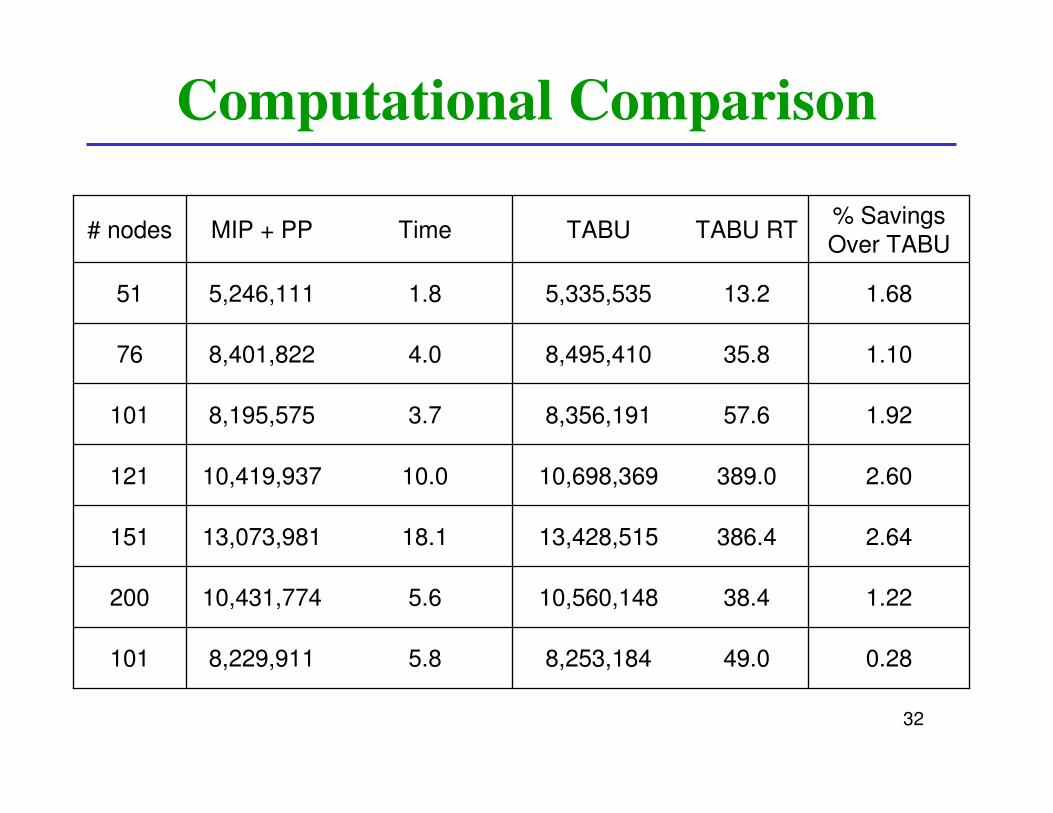
Old Benchmark Problems
� Archetti et al. also solve seven deterministic problems
� These problems resemble scenario 1 or scenario 2 in that demands are small relative to vehicle capacity
� We compare Tabu with MIP + PP on the next page
� MIP + PP clearly outperforms Tabu
32
Computational Comparison
1.2238.410,560,1485.610,431,774200
8,253,184
13,428,515
10,698,369
8,356,191
8,495,410
5,335,535
TABU
0.2849.05.88,229,911101
2.64386.418.113,073,981151
2.60389.010.010,419,937121
1.9257.63.78,195,575101
1.1035.84.08,401,82276
1.6813.21.85,246,11151
% Savings
Over TABUTABU RTTimeMIP + PP# nodes

33
Parameters in Endpoint MIP
� Endpoint MIP has two parameters
� the number of neighbor endpoints
� a time limit
� We set these parameters in order to approximately equalize the running times of Tabu and MIP + PP
34
Other Issues
� There are few SDVRP benchmark problems in the literature
� We’ve created an additional 21 benchmark problems
ranging in size from 8 to 288 nodes
� Using symmetry and geometry, we can visualize a near-
optimal solution for each of these 21 problems
35
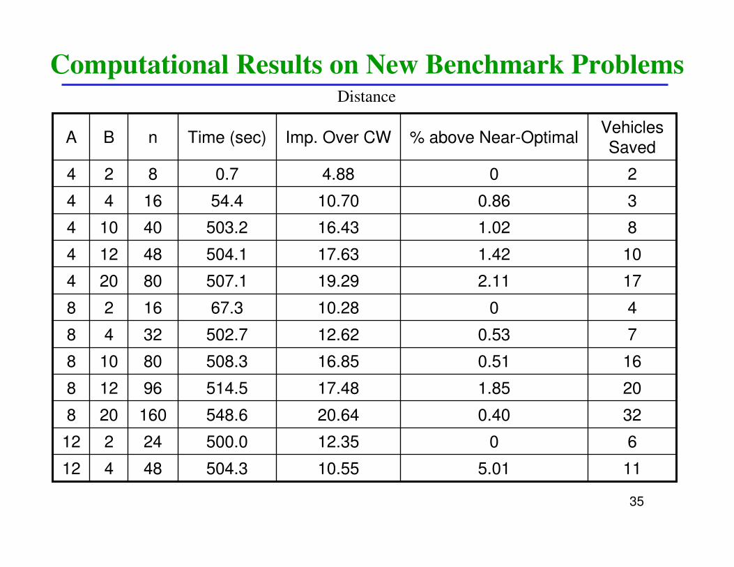
Computational Results on New Benchmark ProblemsDistance
172.1119.29507.180204
160.5116.85508.380108
70.5312.62502.73248
201.8517.48514.596128
81.0216.43503.240104
30.8610.7054.41644
101.4217.63504.148124
115.0110.55504.348412
6012.35500.024212
320.4020.64548.6160208
4010.2867.31628
204.880.7824
Vehicles
Saved% above Near-OptimalImp. Over CWTime (sec)nBA

36
Computational Results on New Benchmark ProblemsDistance
250.9416.49521.71201012
441.4319.82563.02402012
351.5817.00541.61601016
142.7413.80500.064416
402.0617.43554.21921216
290.8018.41542.31441212
651.9620.20651.0288472
342.0020.16514.7144272
8013.42508.332216
Vehicles
Saved% above Near-OptimalImp. Over CWTime (sec)nBA
37
Conclusions and Future Work
� MIP + PP seems to work well
� It consistently outperforms Tabu
� The approach of using MIP to improve a feasible solution
could be applied to other combinatorial optimization
problems
� The robustness of MIP + PP needs to be tested more
comprehensively
� Parameter values need to be determined automatically
� It would be nice to know if the visualized “near-optimal”
solutions are optimal