The Special Theory of Relativity

Albert Einstein

(1879 - 1955)

November 9, 2001

Contents

1 Einstein’s Two Postulates 1

1.1 Galilean Invariance . . . . . . . . . . . . . . . . . . . . . . . . . . . . 2

1.2 The difficulty with Galilean Invariance . . . . . . . . . . . . . . . . . 4

2 Simultaneity, Separation, Causality, and the Light Cone 6

2.1 Simultaneity . . . . . . . . . . . . . . . . . . . . . . . . . . . . . . . . 6

2.2 Separation and Causality . . . . . . . . . . . . . . . . . . . . . . . . . 7

2.3 The Light Cone . . . . . . . . . . . . . . . . . . . . . . . . . . . . . . 8

2.4 The invariance of Separation . . . . . . . . . . . . . . . . . . . . . . . 10

3 Proper time 11

3.1 Proper Time of an Oscillating Clock . . . . . . . . . . . . . . . . . . 13

4 Lorentz Transformations 14

4.1 Motivation . . . . . . . . . . . . . . . . . . . . . . . . . . . . . . . . . 14

4.2 Derivation . . . . . . . . . . . . . . . . . . . . . . . . . . . . . . . . . 15

4.3 Elapsed Proper Time Revisited . . . . . . . . . . . . . . . . . . . . . 17

4.4 Proper Length and Length Contraction . . . . . . . . . . . . . . . . . 18

1

5 Transformation of Velocities 20

5.1 Aberration of Starlight . . . . . . . . . . . . . . . . . . . . . . . . . . 22

6 Doppler Shift 23

6.1 Stellar Red Shift . . . . . . . . . . . . . . . . . . . . . . . . . . . . . 26

7 Four-tensors and all that 27

7.1 The Metric Tensor . . . . . . . . . . . . . . . . . . . . . . . . . . . . 30

7.2 Differential Operators . . . . . . . . . . . . . . . . . . . . . . . . . . . 33

7.3 Notation . . . . . . . . . . . . . . . . . . . . . . . . . . . . . . . . . . 35

8 Representation of the Lorentz transformation 35

9 Covariance of Electrodynamics 40

9.1 Transformations of Source and Fields . . . . . . . . . . . . . . . . . . 40

9.1.1 ρ and J . . . . . . . . . . . . . . . . . . . . . . . . . . . . . . 40

9.1.2 Potentials . . . . . . . . . . . . . . . . . . . . . . . . . . . . . 42

9.1.3 Fields, Field-Strength Tensor . . . . . . . . . . . . . . . . . . 43

9.2 Invariance of Maxwell Equations . . . . . . . . . . . . . . . . . . . . . 45

10 Transformation of the electromagnetic field 46

10.1 Fields Due to a Point Charge . . . . . . . . . . . . . . . . . . . . . . 48

In this chapter we depart temporarily from the study of electromagnetism to ex-

plore Einstein’s special theory of relativity. One reason for doing so is that Maxwell’s

field equations are inconsistent with the tenets of “classical” or “Galilean” relativity.

After developing the special theory, we will apply it to both particle kinematics and

electromagnetism and will find that Maxwell’s equations are completely consistent

with the requirements of the special theory.

2

1 Einstein’s Two Postulates

Physical phenomena may be observed and/or described relative to any of an infinite

number of “reference frames;” we regard the reference frame as being that one relative

to which the measuring apparatus is at rest. The basic claim (or postulate) of rela-

tivity, which predates Einstein’s work by many centuries, is that physical phenomena

should be unaffected by the choice of the frame from which they are observed. This

statement is quite vague. A simple explicit example is a collision of two objects. If

they are seen to collide when observed from one frame, then the postulate of relativity

says that they will be seen to collide no matter what reference frame is used to make

the observation.

1.1 Galilean Invariance

Given that one believes some version of the postulate of relativity, then that person

should, when constructing an explanation of the phenomena in question, make a

theory which will predict the same phenomena in all reference frames. The original

great achievements of this kind were Newton’s theories of mechanics and gravitation.

Consider, for example, F = ma. If the motion of some massive object is observed

relative to two different reference frames, the motion will obey this equation in both

frames provided the frames themselves are not being accelerated. This qualification

leads one to restrict the statement of the relativity principle to unaccelerated or

inertial reference frames.

In order to test the postulate of relativity, one needs a transformation that makes

it possible to translate the values of physical observables from one frame to another.

Consider two frames K and K ′ with K ′ moving at velocity v relative to K.

3

K K’v

vt

x x’

Figure 1: Inerital frames K and K ′

Then the (almost obvious) way to relate a space-time point (t,x) in K to the same

point (t′,x′) in K ′ is via the Galilean transformation

x′ = x− vt and t′ = t, (1)

or so it was believed up to the time of Einstein. Notice that the transformation is

written so that the (space) origins coincide at t = t′ = 0; we shall say simply that the

origins (in space and time) coincide.

In what sense is Newton’s law of motion consistent with the Galilean transforma-

tion? If his equation satisfies the postulate of relativity, then the motion of a massive

object must obey it in both frames; thus

F = ma and F′ = m′a′ (2)

where primed quantities are measured in K ′ and unprimed ones in K. Now, ex-

periments demonstrate (not quite correctly) that the force and mass are invariants,

meaning that they are the same in all inertial frames, so if Newton’s law is to hold in

all inertial frames, then it must be the case that a = a′. The Galilean transformation

provides a way of comparing these two quantities. In Eqs. (1), let x and x′ be the

positions of the mass at, respectively, times t and t′ in frames K and K ′. Then we

4

havedx′

dt′=dx

dt− v (3)

and

a′ =d2x′

dt′2=d2x

dt2= a, (4)

assuming v is a constant. Thus we find that Newton’s law, Galileo’s transformation,

and the observed motions of massive objects are consistent. 1.

1.2 The difficulty with Galilean Invariance

Now we come to the dilemma posed by Maxwell’s equations. They are not consistent

with the postulate of relativity if one uses the Galilean transformation to relate quan-

tities in two different inertial frames. Imagine the quandary of the late-nineteenth-

century physicist. He had the Galilean transformation and Newton’s equations of mo-

tion, backed by enormous experimental evidence, to support the almost self-evident

principle of relativity. But he also had the new - and enormously successful - Maxwell

theory of light which was not consistent with Galilean relativity. What to do? One

possible way out of the morass was easy to find. It was well-known that wavelike

phenomena, such as sound, obey wave equations which are not properly “invariant”

under Galilean transformations. The reason is simple: These waves are vibrational

motions of some medium such as air or water, and this medium will be in motion

with different velocities relative to the coordinate axes of different inertial frames. If

one understood this, then one could see that although the wave equation takes on

different forms relative to different frames, it did correctly describe what goes on in

every frame and was not inconsistent with the postulate of relativity.

The appreciation of this fact set off a great search to find the medium, called

the “luminiferous ether” or simply the ether, whose vibrations constitute electromag-

1Of course, they aren’t consistent at all if one either makes measurements of extraordinary

precision or studies particles traveling at an appreciable fraction of the speed of light. Neither of

these things was done prior to the twentieth century.

5

netic waves. The search (i.e. Michelson and Morely) was, as we know, completely

unsuccessful2, as the ether eluded all seekers.

However, for Einstein, it was the Fizeau experiment (1851) which convinced him

that the ether explaination was incorrect. This experiment looked for a change in

the phase velocity of light due to its passage through a moving medium, in this case

water.

mirrors

Transparent pipe, filledwith flowing water.

light

light

Figure 2: Diagram of Fizeau experiment

Fitzeau found that this phase velocity was given by

vphase =c

n± v

(1− 1

n2

)experiment

where n is the index of refraction of the water, and v is its velocity. The plus(minus)

sign is taken if the water is moving with(against) the light.

Lets analyze the experiment from a Galilean point of view. The dielecric water

is moving in either the same or opposite direction as the light, and so acts as a

moving source for the light with is refracted (i.e. reradiated by the water molecules).

Nonrelativistically, we just add the velocity v of the source to the wave velocity for

the stationary source. Thus Galilean therory says

vphase =c

n± v Galilean theory,

2Or completely successful, if we adopt a somewhat different (Einstein’s) point of view.

6

which is clearly inconsistent with experiment.

The stage was now set for Einstein who, in 1905, made the following postulates:

1. Postulate of relativity: The laws of nature and the results of all experiments

performed in a given frame of reference are independent of the translational

motion of the system as a whole.

2. Postulate of the constancy of the speed of light: The speed of light is indepen-

dent of the motion of its source.

The first postulate essentially reaffirmed what had long been thought or believed in

the specific case of Newton’s law, extending it to all phenomena. The second postulate

was much more radical. It did away with the ether at a stroke and also with Galilean

relativity because it implies that the speed of light is the same in all reference frames

which is fundamentally inconsistent with the Galilean transformation.

2 Simultaneity, Separation, Causality, and the Light

Cone

2.1 Simultaneity

The second postulate - disturbing in itself - leads to many additional “nonintuitive”

predictions. For example, suppose that there are sources of light at points A and C

and that they both emit signals that are observed by someone at B which is midway

between A and C.

7

A B C

CBA v

B was herewhen the signalswere emitted.

Figure 3: Simultaneity depends upon the rest frame of the observer

If he sees the two signals simultaneously and knows that he is equidistant from the

sources, he will conclude quite correctly that the signals were emitted simultaneously.

Now suppose that there is a second observer, B’,who is moving along the line from

A to C and who arrives at B just when the signals do. He will know that the signals

were emitted at some earlier time when he was closer to A than to C. Also, since

both signals travel with the same speed c in his rest frame (because the speeds of the

signals relative to him are independent of the speeds of the sources relative to him),

he will conclude that the signal from C was emitted earlier than that from A because

it had to travel the greater distance before reaching him. He is as correct as the first

observer. Similarly, an observer moving in the opposite direction relative to the first

one will conclude from the same reasoning that the signal from A was emitted before

that from C. Hence Einstein’s second postulate leads us to the conclusion that events,

in this case the emission of light signals, which are simultaneous in one inertial frame

are not necessarily simultaneous in other inertial frames.

2.2 Separation and Causality

If simultaneity is only a relative fact, as opposed to an absolute one, what about

causality? Because the order of the members of some pairs of events can be reversed

by changing one’s reference frame, we must consider whether the events’ ability to

8

influence each other can similarly be affected by a change of reference frame. This

question is closely related to a quantity that we shall call the separation between

the events. Given two events A and B which occur at space-time points (t1,x1) and

(t2,x2), we define the squared separation s212 between them to be

s212 ≡ c2(t1 − t2)2 − |x1 − x2|2. (5)

Let the two events be (1) the emission of an electromagnetic signal at some point in

vacuum and (2) its reception somewhere else. Then, because the signal travels with

the speed c, these events have separation zero, s212 = 0. This result will be the same

in any inertial frame since the signal has the same speed c in all such frames.

Now, if we have two events such that s212 > 0, then we have a “causal relationship”

in the sense that a light signal can get from the first event to the place where the

second one occurs before it does occur. Such a separation is called timelike. On

the other hand, if s212 < 0, then a light signal cannot get from the first event to the

location of the second event before the second event occurs. This separation is called

spacelike. A separation s212 = 0 is called lightlike.

It is important to ask whether there is some other type of signal that travels faster

than c and which could therefore produce a causal relationship between events with

a spacelike separation. None has been found and we shall assume that none exists.

Consequently, we claim that events with a timelike separation are such that the earlier

one can influence the later one, because a signal can get from the first to the location

of the second before the latter occurs, but that events with a spacelike separation are

such that the earlier one cannot influence the later one because a signal cannot get

from the first event to the location of the second one fast enough.

2.3 The Light Cone

The question now is whether the character of the separation between two events,

timelike, spacelike, or lightlike, can be changed by changing the frame in which it is

9

measured. For simplicity, let the “first” event, A, occur (in frame K) at (t = 0,x = 0)

while the second takes place at some general (t,x) with t > 0. Further, let ct be larger

than |x| so that s2 > 0 and A may influence B. Consider these same two events in

another frame K ′. By an appropriate choice of the origin (in space and time) of this

frame, we can make the first event occur here, just as it does in frame K. The second

event will be at some (t’,x’).

We can picture the relative positions of the two events in space and time by using

a light cone as shown.

future

ct

| |xA

B

elsewhere

pasts < 0

s > 0

2

2

Figure 4: The Light Cone

The vertical axis measures ct; the horizontal one, separation in space, |x|. The two

diagonal lines have slopes ±1. The event B is shown within the cone whose axis is

the ct axis; any event with a timelike separation relative to the origin will be in here.

The question we wish to ask now is whether, by going to another reference frame,

one may cause event B to move across one of the diagonal lines and so wind up in

a place where it cannot be influenced by the event at the origin? The point is that

A can influence any event inside of the “future” cone; it can be influenced by any

event inside of the “past” cone; but it cannot influence, or be influenced by, any event

inside of the “elsewhere” region. If an event B and two reference frames K and K ′

can be found such that the event when expressed in one frame is on the opposite

side of a diagonal from where it is in the other frame, then we have made causality a

frame-dependent concept.

Suppose that we have two such frames. We can effect a transformation from one

to the other by considering a sequence of many frames, each moving at a velocity only

10

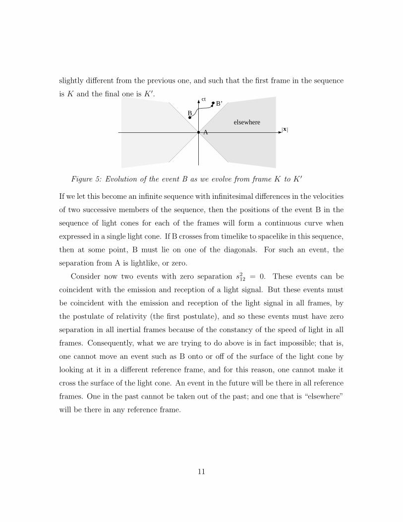
slightly different from the previous one, and such that the first frame in the sequence

is K and the final one is K ′.ct

| |xA

Belsewhere

B’

Figure 5: Evolution of the event B as we evolve from frame K to K ′

If we let this become an infinite sequence with infinitesimal differences in the velocities

of two successive members of the sequence, then the positions of the event B in the

sequence of light cones for each of the frames will form a continuous curve when

expressed in a single light cone. If B crosses from timelike to spacelike in this sequence,

then at some point, B must lie on one of the diagonals. For such an event, the

separation from A is lightlike, or zero.

Consider now two events with zero separation s212 = 0. These events can be

coincident with the emission and reception of a light signal. But these events must

be coincident with the emission and reception of the light signal in all frames, by

the postulate of relativity (the first postulate), and so these events must have zero

separation in all inertial frames because of the constancy of the speed of light in all

frames. Consequently, what we are trying to do above is in fact impossible; that is,

one cannot move an event such as B onto or off of the surface of the light cone by

looking at it in a different reference frame, and for this reason, one cannot make it

cross the surface of the light cone. An event in the future will be there in all reference

frames. One in the past cannot be taken out of the past; and one that is “elsewhere”

will be there in any reference frame.

11

2.4 The invariance of Separation

With a little more thought we can generalize the conclusion of the previous paragraph

that two events with zero separation in one frame have zero separation in all frames.

In fact, the separation, whatever it may be, between any two events is the same in

all frames. We shall call something that is the same in all frames an invariant; the

separation is an invariant. To argue that this should be the case, suppose that we

have two events which are infinitesimally far apart in both space and time so that we

may write ds12 for s12,

(ds12)2 = c2(t1 − t2)2 − |x1 − x2|2 (6)

in frame K. In another inertial frame K ′ we have separation (ds′12)2, and we have

argued that this is zero if ds212 is zero. If K ′ is moving with a small speed relative to

K, the separations in the two frames must be nearly equal which means that they

will be infinitesimal quantities of the same order, or

(ds12)2 = A(ds′12)2 (7)

where A = A(v) is a finite function of v, the relative speed of the frames. Furthermore,

A(0) = 1 since the two frames are the same if v = 0. Now, if time and space are

homogeneous and isotropic, then it must also be true that

(ds′12)2 = A(v)(ds12)2. (8)

Comparing the preceding equations, we see that the only solutions are A(v) = ±1;

the condition that A(0) = 1 means A(v) = 1. Hence

(ds′12)2 = (ds12)2 (9)

which is a relation between differentials that may be integrated to give

(s′12)2 = (s12)2, (10)

12

thereby demonstrating that the separation between any two events is an invariant.

The locus of all points with a given separation is a hyperbola when drawn on a light

cone (or a hyperboloid of revolution if more spatial dimensions are displayed in the

light cone).

3 Proper time

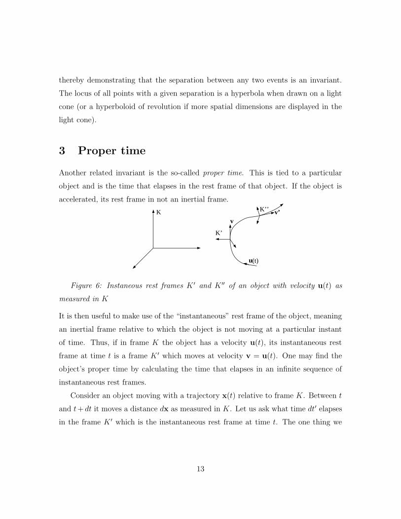
Another related invariant is the so-called proper time. This is tied to a particular

object and is the time that elapses in the rest frame of that object. If the object is

accelerated, its rest frame in not an inertial frame.

K

u(t)

K’

vv’K’’

Figure 6: Instaneous rest frames K ′ and K ′′ of an object with velocity u(t) as

measured in K

It is then useful to make use of the “instantaneous” rest frame of the object, meaning

an inertial frame relative to which the object is not moving at a particular instant

of time. Thus, if in frame K the object has a velocity u(t), its instantaneous rest

frame at time t is a frame K ′ which moves at velocity v = u(t). One may find the

object’s proper time by calculating the time that elapses in an infinite sequence of

instantaneous rest frames.

Consider an object moving with a trajectory x(t) relative to frame K. Between t

and t+ dt it moves a distance dx as measured in K. Let us ask what time dt′ elapses

in the frame K ′ which is the instantaneous rest frame at time t. The one thing we

13

know is that

(ds)2 ≡ c2(dt)2 − (dx)2 = (ds′)2 = c2(dt′)2 − (dx′)2 (11)

where, as usual, unprimed quantities are the ones measured relative to K and primed

ones are measured in K ′. Now, dx′ = 03 because the object is at rest in K ′ at time t.

Hence we may drop this contribution to the (infinitesimal) separation and solve for

dt′:

dt′ =√

(dt)2 − (dx)2/c2 = dt

√√√√1− 1

c2

(dx

dt

)2

= dt√

1− u2/c2 (12)

where u ≡ dx/dt is the object’s velocity as measured in K. Now we may integrate

from some initial time t1 to a final time t2 to find the proper time of the object which

elapses while time is proceeding from t1 to t2 in frame K; that is, we are adding up

all of the time that elapses in an infinite sequence of instantaneous rest frames of the

object while time is developing in K from t1 to t2.

τ2 − τ1 =∫ t2

t1dt√

1− u2(t)/c2. (13)

3.1 Proper Time of an Oscillating Clock

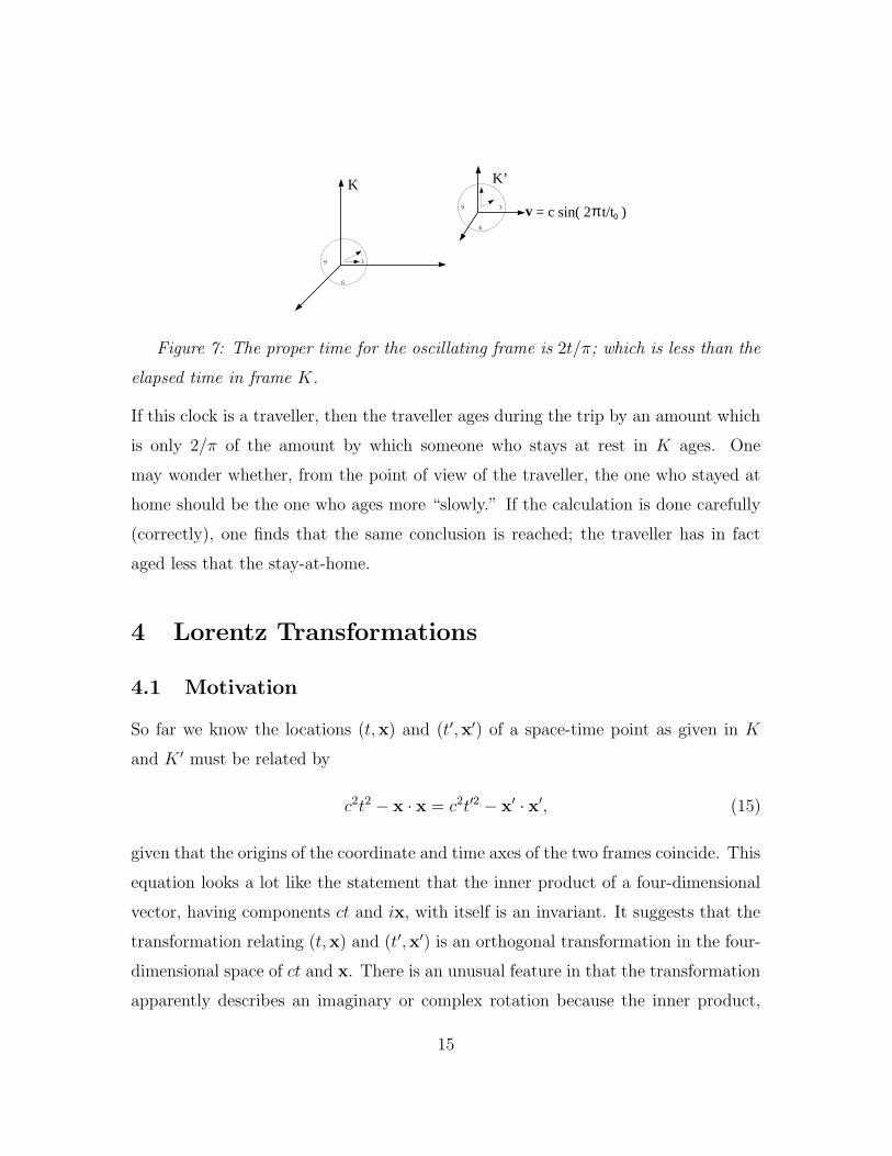
As an example let the object move along a one-dimensional path with u(t) = c sin(2πt/t0)

with t1 = 0 and t2 = t0. This velocity describes a round trip of a harmonic oscillator

with a peak speed of c and a period of t0. The corresponding elapsed proper time is

τ0 =∫ t0

0dt√

1− sin2(2πt/t0) =∫ t0

0dt | cos(2πt/t0)| = 2t0/π. (14)

This is smaller than t0 by a factor of 2/π which means that a clock carried by the

object will show an elapsed time during the trip which is just 2/π times what a clock

which remains in frame K will show, provided the acceleration experienced by the

clock which makes the trip doesn’t alter the rate at which it runs.

3More correctly dx′ is a second order differential, and hence may be neglected

14

K K’

v3

6

9 = c sin( 2 t/t )π 0

3

6

9

Figure 7: The proper time for the oscillating frame is 2t/π; which is less than the

elapsed time in frame K.

If this clock is a traveller, then the traveller ages during the trip by an amount which

is only 2/π of the amount by which someone who stays at rest in K ages. One

may wonder whether, from the point of view of the traveller, the one who stayed at

home should be the one who ages more “slowly.” If the calculation is done carefully

(correctly), one finds that the same conclusion is reached; the traveller has in fact

aged less that the stay-at-home.

4 Lorentz Transformations

4.1 Motivation

So far we know the locations (t,x) and (t′,x′) of a space-time point as given in K

and K ′ must be related by

c2t2 − x · x = c2t′2 − x′ · x′, (15)

given that the origins of the coordinate and time axes of the two frames coincide. This

equation looks a lot like the statement that the inner product of a four-dimensional

vector, having components ct and ix, with itself is an invariant. It suggests that the

transformation relating (t,x) and (t′,x′) is an orthogonal transformation in the four-

dimensional space of ct and x. There is an unusual feature in that the transformation

apparently describes an imaginary or complex rotation because the inner product,

15

or length, that is preserved is c2t2 − x · x as opposed to c2t2 + x · x. Recall that a

rotation in three dimensions around the ε3 direction by angle φ can be represented

by a matrix

a =

cosφ − sinφ 0

sinφ cosφ 0

0 0 1

(16)

so that

x′i =3∑

j=1

aijxj; (17)

that is,

x′1 = cosφx1 − sinφx2

x′2 = sinφx1 + cosφx2

x′3 = x3.

(18)

For an imaginary φ, φ = iη, cosφ → cosh η, and sinφ → −i sinh η. Further, let us

reconstruct the vector as y = (x1, ix2, ix3) and make the transformation

y′i =∑

j

aijyj. (19)

The result, expressed in terms of components of x, is

x′1 = cosh η x1 − sinh η x2

x′2 = − sinh η x1 + cosh η x2

x′3 = x3;

(20)

these are such that

x′21 − x′22 − x′23 = x21 − x2

2 − x23 (21)

since cosh2(η)− sinh2(η) = 1, so we have succeeded in constructing a transformation

that produces the right sort of invariant. All we have to do is generalize to four

dimensions.

16

4.2 Derivation

Let’s begin by introducing a vector with four components, (x0, x1, x2, x3) where x0 =

ct and the xi with 1 = 1, 2, 3 are the usual Cartesian components of the position

vector. Then introduce ~y ≡ (x0, ix) which has the property that

~y · ~y = x20 − x · x. (22)

This inner product is supposed to be an invariant under the transformation of x and

t that we seek. The transformation in question is a rotation through an imaginary

angle iη that mixes time and one spatial direction, which we pick to be the first (y1

or x1) without loss of generality. The matrix representing this rotation is

a =

cosh η i sinh η 0 0

−i sinh η cosh η 0 0

0 0 1 0

0 0 0 1

. (23)

Now operate with this matrix on ~y to produce ~y′. If we write the components of the

latter as (x′0, ix′), we find the following:

x′0 = cosh η x0 − sinh η x1

x′1 = − sinh η x0 + cosh η x1

x′2 = x2

x′3 = x3.

(24)

It is a simple matter to show from these results that x20 − x · x is an invariant, i.e.,

x20 − x · x = x′20 − x′ · x′ (25)

which means we have devised an acceptable transformation in the sense that it pre-

serves the separation between two events.

But what is the significance of η? Let us rewrite sinh η as cosh η tanh η. Then we

have, in particular,

x′0 = cosh η (x0 − tanh η x1)

x′1 = cosh η (x1 − tanh η x0).(26)

17

The second of these is

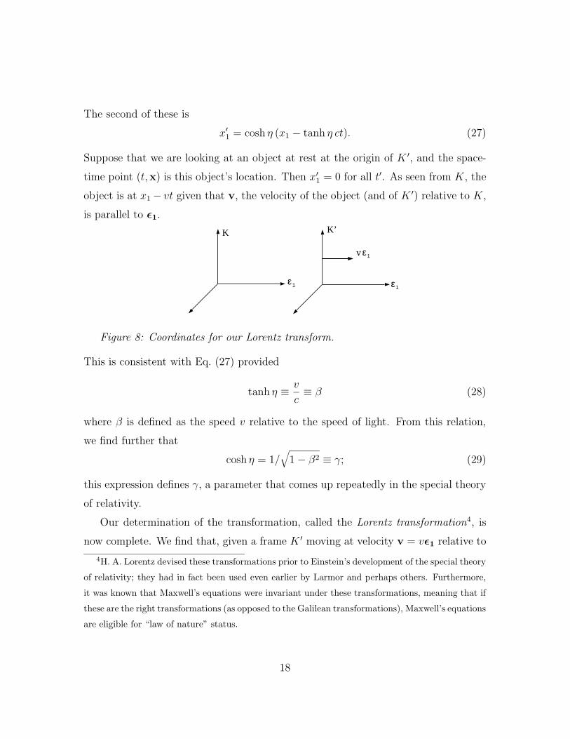
x′1 = cosh η (x1 − tanh η ct). (27)

Suppose that we are looking at an object at rest at the origin of K ′, and the space-

time point (t,x) is this object’s location. Then x′1 = 0 for all t′. As seen from K, the

object is at x1− vt given that v, the velocity of the object (and of K ′) relative to K,

is parallel to ε1.

K K’

ε1

ε1v

ε1

Figure 8: Coordinates for our Lorentz transform.

This is consistent with Eq. (27) provided

tanh η ≡ v

c≡ β (28)

where β is defined as the speed v relative to the speed of light. From this relation,

we find further that

cosh η = 1/√

1− β2 ≡ γ; (29)

this expression defines γ, a parameter that comes up repeatedly in the special theory

of relativity.

Our determination of the transformation, called the Lorentz transformation4, is

now complete. We find that, given a frame K ′ moving at velocity v = vε1 relative to

4H. A. Lorentz devised these transformations prior to Einstein’s development of the special theory

of relativity; they had in fact been used even earlier by Larmor and perhaps others. Furthermore,

it was known that Maxwell’s equations were invariant under these transformations, meaning that if

these are the right transformations (as opposed to the Galilean transformations), Maxwell’s equations

are eligible for “law of nature” status.

18

K, a space-time point (t,x) in K becomes, in K ′, the space-time point (t′,x′) with

x′0 = γ(x0 − βx1) x′1 = γ(x1 − βx0) x′2 = x2 x′3 = x3. (30)

The inverse transformation can be extracted from these equations in a straightforward

manner; it may also be inferred from the fact that K is moving at velocity −v relative

to K ′ which tells us immediately that

x0 = γ(x′0 + βx′1) x1 = γ(x′1 + βx′0) x2 = x′2 x3 = x′3. (31)

4.3 Elapsed Proper Time Revisited

Let us try to use this transformation to calculate something. First, we revisit the

proper time. For an object at rest in K ′, x′ does not change with time. Also, from

our transformation,

ct = γ(ct′ + βx′1), (32)

The differential of this transformation, making use of the fact that the object is

instantaneously at rest in K ′, gives, dt = γdt′ since dx′1 is second-order in powers of

dt′. Stated in another fashion, we are considering the transformation of two events

or space-time points. They are the locations of the object at times t′ and t′ + dt′.

Because the object is at rest in K ′ at time t′, its displacement dx′ during the time

increment dt′ is of order (dt′)2 and so may be discarded. The corresponding elapsed

time dt in K is thus found to be dt = γdt′, using the Lorentz transformations of the

two space-time points. This equation may also be written as

dt′ = dt/γ =√

1− v2/c2dt. (33)

The left-hand side of this equation is the elapsed proper time of the object while dt

is the elapsed time measured by observers at rest relative to K. If we introduce u,

the velocity of the object relative to K, and notice that u = v at time t, then we can

write dt′ in terms of u(t) as

dt′ =√

1− |u(t)|2/c2dt, (34)

19

where now dt′ in the elapsed proper time of the object which moves at velocity u

relative to frame K. We can integrate this relation to find the finite elapsed proper

time during an arbitrary time interval (in K),

τ2 − τ1 =∫ t2

t1dt√

1− |u(t)|2/c2. (35)

4.4 Proper Length and Length Contraction

Next, we shall examine the Fitzgerald-Lorentz contraction. Define the proper length

of an object as its length, measured in the frame where it is at rest. Let this be L0,

and let the rest frame be K ′, moving at the usual velocity (v = vε1) relative to K.

K K’

ε1

ε1v

ε1

0L

Figure 9: Length contraction occurs along the axis parallel to the velocity.

The relative geometry is shown in the figure. The rod, or object, is positioned in K ′

so that its ends are at x′1 = 0, L0. They are there for all t′. In order to find the length

of the rod in K, we have to measure the positions of both ends at the same time t

as measured in K. We can find the results of these measurements from the Lorentz

transformation

x′1 = γ(x1 − βx0). (36)

Use this relation first with x′1 equal to 0 and then with x′1 = L0, using the same time

x0 in both cases, and take the difference of the two equations so obtained. The result

is

L0 = γ(x1R − x1L) ≡ γL (37)

where x1R and x1L are the positions of the right and left ends of the rod at some

20

particular time, or x0. The difference of these is L, the length of the rod as measured

in frame K.

Our result for L can be written as

L = L0/γ =√

1− β2L0. (38)

This length is smaller than L0 which means that the object is found (is measured)

in K to be shorter than its proper length or its length in the frame where it is at

rest. Notice, however, that if we did the same calculation for its length in a direction

perpendicular to the direction of v, we would find that it is the same in K as in K ′.

Consequently the transformation of the object’s volume is

V = V0/γ =√

1− β2 V0 (39)

where V0 is the proper volume or volume in the rest frame, and V is the volume in a

frame moving at speed βc relative to the rest frame.

5 Transformation of Velocities

Because we know how x and t transform, we can determine how anything that involves

functions of these things transforms. For example, velocity. Let an object have

velocity u in K and velocity u′ in K ′ and let K ′ move at velocity v relative to K.

We wish to determine how u′ is related to u. In K ′, the object moves a distance

dx′ = u′dt′ in time dt′. A similar statement, without any primed quantities, holds

in K. The infinitesimal displacements in time and space are related by Lorentz

transformations:

dt = γ(v)(dt′ + (v/c2)dx′

)dx = γ(v)(dx′+vdt′) dy = dy′ dz = dz′,

(40)

where we have let v be along the direction of x1 as usual. Taking ratios of the

displacements to the time increment, we have

ux =dx

dt=

dx′ + vdt′

dt′ + (v/c2)dx′=

dx′/dt′ + v

1 + (v/c2)(dx′/t′)=

u′x + v

1 + vu′x/c2, (41)

21

uy =1

γ(v)

u′y1 + vu′x/c

2, (42)

and

uz =1

γ(v)

u′z1 + vu′x/c

2. (43)

These results may be summarized in vectorial form:

u‖ =u′‖ + v

1 + v · u′/c2u⊥ =

u′⊥γ(v)(1 + v · u′/c2)

(44)

where the subscripts “‖” and “⊥” refer respectively to the components of the velocities

u and u′ parallel and perpendicular to v. Notice too that

u‖ =(

u · vv2

)v and u⊥ = u− u‖ = u−

(u · vv2

)v. (45)

It is sometimes useful to express the transformations for velocity in polar coordi-

nates (u, θ) and (u′, θ′) such that

u‖ = u cos θ and u⊥ = u sin θ, (46)

etc.; the appropriate expressions are

tan θ =u′ sin θ′

γ(v)(u′ cos θ′ + v)and u =

[u′2 + v2 + 2u′v cos θ′ − (vu′ sin θ′/c)2]1/2

1 + u′v cos θ′/c2.

(47)

K K’

ε1

ε1vθ

θ’ u

u’

Figure 10: Frames for velocity transform.

The inverses of all of these velocity transformations are easily found by appropriate

symmetry arguments based on the fact that the velocity of K relative to K ′ is just

−v.

22

In it interesting that the velocity transformations are, in contrast to the ones for

x and t, nonlinear. They must be nonlinear because there is a maximum velocity

which is the speed of light; combining two velocities, both of which are close to, or

equal to, c, cannot give a velocity greater than c. A linear transformation would

necessarily allow this to happen, so a nonlinear transformation is required. To see

how the transformations rule out finding a frame where an object moves faster than c,

let us consider the transformation of a velocity |u′| = c. From the second of Eqs. (47),

we see that

u =c2 + v2 + 2cv cos θ′ − v2(1− cos2 θ′)]1/2

1 + v cos θ′/c= c

[(1 + v cos θ′/c)2]1/2

1 + v cos θ′/c= c. (48)

Thus do we find what we already knew: If something moves at speed c in one frame,

then it moves at the same speed in any other frame. More generally, if we had used

any u′ ≤ c and v ≤ c, we would have recovered a u ≤ c.

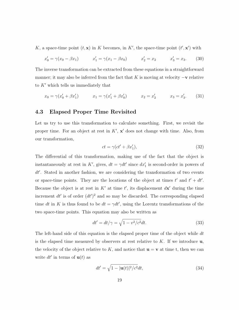
5.1 Aberration of Starlight

An interesting example of the application of the velocity transformation is the ob-

served aberration of starlight. Suppose that an observer is moving with speed v at

right angles to the direction of a star that he is watching. If a Galilean transformation

is applied to the determination of the apparent direction of the star, one finds that

it is seen at an angle φ away from its true direction where tanφ = v/c.

Sol

planet

vstar c

φ

tan( ) =v/cφ (Galilean)

23

Figure 11: Due to the finite velocity of light, a star is seen an angle φ away from

its true direction.

One can measure this angle by waiting six months. The velocity v is provided by

the earth’s orbital motion; six months later it is reversed and if the observer then

looks for the same star, it position will have shifted by 2φ, at least according to the

Galilean transformation.

But that prediction is not correct. Consider what happens if the Lorentz trans-

formation is used to compute the angle φ. Using Eq. (47), we see that the angle θ at

which the light from the star appears to be headed in the frame K of the observer is

tan θ =c sin θ′

√1− v2/c2

c(cos θ′ + v/c). (49)

where θ′ is its direction in the frame K ′ which is the rest frame of the sun.

φ

θ θ’

v

K’K

=π/2

φ = π/2 − θ

Figure 12: Coordinates for stargazing.

Now suppose that v is at π/2 radians to the direction of the light’s motion in frame

K ′ so that θ′ = π/2. Then we find tan θ = c/γ(v)v. To compare with the prediction

of the Galilean transformation, we need to find the angle φ, which is to say, π/2− θ.From a trigonometric identity, we have

tan θ =tan(π/2)− tanφ

1 + tan(π/2) tanφ=

1

tanφ, (50)

and so

tanφ = vγ(v)/c or sinφ = v/c. (51)

24

This is the correct answer; the tangent of the angle φ differs from the prediction of

the Galilean transformation by a factor of γ which is second-order in powers of v/c.

6 Doppler Shift

The Doppler shift of sound is a well-known and easy to understand phenomenon. It

depends on the velocities of the source and observer relative to the medium in which

the waves propagate. For electromagnetic waves, this medium does not exist and so

the Doppler shift for light takes on its own special - and relatively simple! - form.

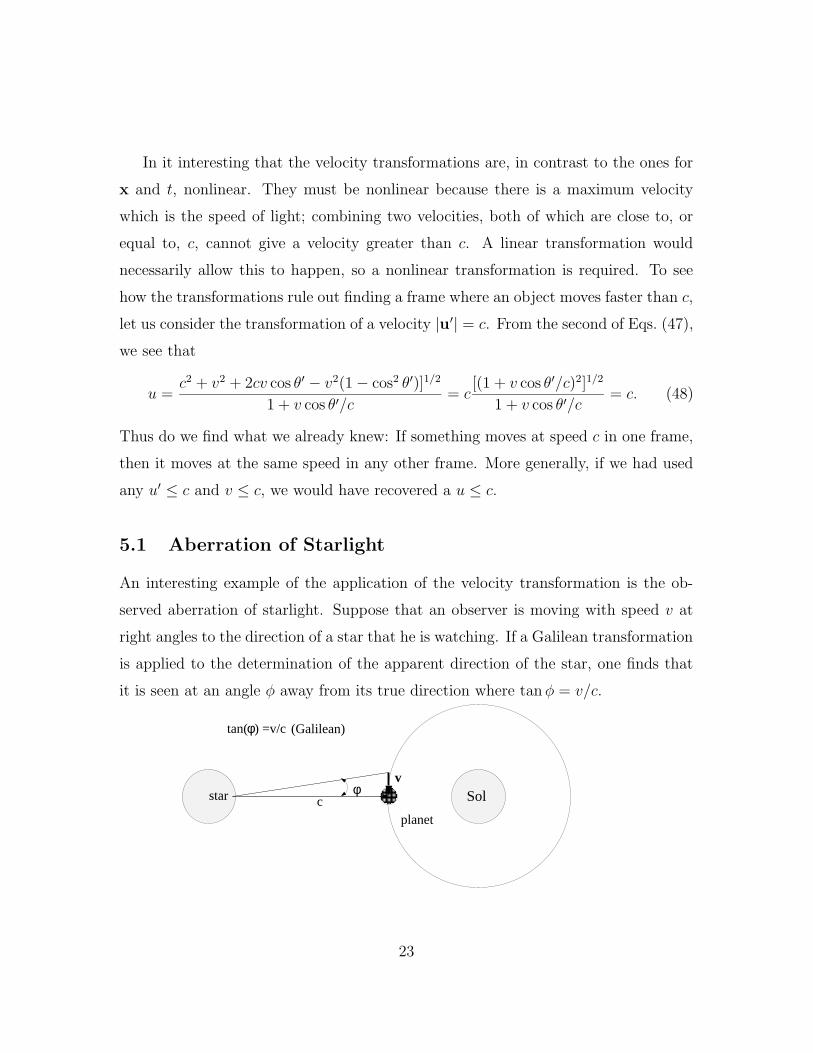
Suppose that in frame K there is a plane wave with wave vector k and frequency

ω. Put an observer at some point x and set him to work counting wave crests as they

go past him.

1 2 3 4

K

Figure 13: An observer counts wave crests.

Let him begin with the crest which passes the origin at t = 0 and continue counting

until some later time t. How many crests does he count? We can decide by first

determining when he starts. The starting time is t0 = (k · x)/kvw where vw is the

velocity of the wave in frame K. The observer counts from t0 to t and so counts n

crests where

n = (t− t0)/T ; (52)

T is the period of the wave, T = 2π/ω. Hence,

n =1

2π

(ωt− ω

kvwk · x

)=

1

2π(ωt− k · x), (53)

since ω = vwk.

25

K K’

v

x’x

K’K

v

x’x

t = 0 t = t

Figure 14: Frame alignments for the Doppler problem.

Now let the same measurement be performed by an observer at rest at a point x′

in frame K ′ which moves at v relative to K. We choose x′ in a special way; it must

be coincident with x at time t (measured in K). This observer also counts crests,

starting with the one that passed his origin at time t′ = 0 and stopping with the one

that arrives when he (the second observer) is coincident with the first observer. Given

the usual transformations, the four-dimensional coordinate origins coincide, and so

both observers count the same number of crests. Repeating the argument given for

the number counted by the first observer, we find that the number counted by the

second observer can be written as

n =1

2π(ω′t′ − k′ · x′) (54)

where ω′ and k′ are the frequency and wave vector of the wave in K ′ and (t′,x′) is

the spacetime point that transforms into (t,x). Thus we find

ωt− k · x = ω′t′ − k′ · x′. (55)

The significance of this relation is that the phase of the wave is an invariant. Further

it appears to be the inner product of (ct, ix) and (ω/c, ik). Because we know how

(t,x) transforms to (t′,x′), we can figure out how (ω/c, ik) transforms to (ω ′/c, ik′).

Let ω/c ≡ k0 and ω′/c ≡ k′0 and consider Eq. (55) with the transformations Eq. (30)

used for t′ and x′:

ωt− k1x1 − k2x2 − k3x3 = ω′γ(t− βx1/c)− k′1γ(x1 − βct)− k′2x2 − k′3x3. (56)

26

Because t and x are completely arbitrary, we may conclude that

ω = γ(ω′ + βck′1) k1 = γ(k′1 + βω′/c) k2 = k′2 k3 = k′3, (57)

or

k0 = γ(k′0 + βk′1) k1 = γk′1 + βk′0) k2 = k′2 k3 = k′3. (58)

We recognize the form of these transformations; they tell us that (k0,k) transforms

in the same way as (x0, ix), i.e., via the Lorentz transformation.

Let’s spend a few minutes thinking about the conditions under which our result

is valid. We assumed when making the argument that we have a plane wave in both

K and K ′ which means, more or less, that we are giving Maxwell’s equations Law of

Nature status since we assumed that the relevant equation of motion produces plane

wave solutions in both frames. In fact, our results are not correct for waves in general,

because many types of waves will not have this property (plane waves remain plane

waves relative to all reference frames if they are plane waves relative to one frame).

But they are correct for electromagnetic waves in vacuum.

Finally, let us look at an alternative form for our transformations. Let

k′ = k′(cos θ′ ε1 + sin θ′ ε2); (59)

the component of k′ perpendicular to ε1 is defined to be in the direction of ε2. Further,

k′ = ω′/c. Then the transformation equations may be used to produce the relations

k1 = γk′(cos θ′ + β) k2 = k′ sin θ′ ε2 and ω = γω′(1 + β cos θ′) (60)

where k2 is the component of k which is perpendicular to ε1. ¿From these results it

is easy to show that ω − ck, no surprise, and that

cos θ =cos θ′ + β

1 + β cos θ′; (61)

θ is the angle that k makes with the direction of v, (or ε1); that is,

k = k(cos θ ε1 + sin θ ε2). (62)

27

6.1 Stellar Red Shift

The last of Eqs. (60) in particular may be used to describe the Doppler shift of the

frequency of electromagnetic waves in vacuum. A well-known case in point is the

“redshift” of light from distant galaxies.

K K’

v

starearth

light

Figure 15: Light from receding stars in K ′ is redshifted when seen in K.

Given an object receding from the observer in K and emitting light of frequency ω ′

in its own rest frame, K ′, we have cos θ′ ≈ −1 and

ω = γω′(1− β) = ω′√

1− β1 + β

. (63)

For, e.g., β = 1/2, ω = ω′/√

3. The observer sees the light as having much lower

frequency than that with which it is emitted; it is “red-shifted.”

7 Four-tensors and all that

5 It is no accident that (x0,x) and (k0,k) transform from K to K ′ in the same way.

They are but two of many sets of four objects or elements that have this property.

They are called four-vectors. More generally, there are sets of 4p elements, with

p = 0, 1, 2..., which have very similar transformation properties and which are called

four-tensors of rank p. The better to manipulate them when the time comes, let us

spend a little time now learning some of the basics of tensor calculus.

5The introduction to tensor calculus given in this section is largely drawn from J. L. Synge and

A. Schild, Tensor Calculus, (University of Toronto Press, Toronto, 1949).

28

Consider the usual frames K and K ′ with coordinates x and x′, respectively; x

stands for (x0,x) and similarly for x′. Let there be some transformation from one

frame to the other which gives

x′ = x′(x), (64)

with an inverse,

x = x(x′). (65)

These transformations need not in general be linear.

A contravariant vector or rank-one tensor is defined to be a set of four quan-

tities or elements aα, α = 0, 1, 2, 3, which transform from K to K ′ according to the

rule

a′α =3∑

β=0

∂x′α

∂xβaβ ≡ Aαβa

β. (66)

This equation serves to define Aαβ,

Aαβ ≡∂x′α

∂xβ; (67)

we have also introduced in the last step the summation convention that a Greek

index, which appears in a term as both an upper and a lower index, is summed from

zero to three.

For any contravariant vector or tensor, we are going to introduce also a covariant

vector or tensor whose components will be designated by subscripts. Define a co-

variant vector or rank-one tensor as a set of four objects bα, α = 0, 1, 2, 3, which

transform according to the rule

b′α =3∑

β=0

∂xβ

∂x′αbβ ≡ A β

α bβ (68)

where we have defined

A βα ≡

∂xβ

∂x′α. (69)

The generalization to tensors of ranks other than one is straightforward. For

example, a rank-two contravariant tensor comprises a set of sixteen objects T αβ which

29

transform according to the rule

T ′αβ = AαγAβδT

γδ (70)

and a rank-two covariant tensor has sixteen elements Tαβ which transform according

to the rule

T ′αβ = A γα A

δβ Tγδ. (71)

Mixed tensors can also be of interest. The rank-two mixed tensor T is a set of sixteen

elements T αβ which transform according to

T ′αβ = AαγAδβ T

γδ. (72)

Generalizations follow as you would expect.

The inner product of a and b can be6 defined as

a · b ≡ bαaα. (73)

Consider the transformation properties of the inner product:

a′ · b′ = a′αb′α = A γα A

αδbγa

δ; (74)

however,

A γα A

αδ =

∂xγ

∂x′α∂x′α

∂xδ=∂xγ

∂xδ= δγδ (75)

where

δγδ ≡

1 γ = δ

0 γ 6= δ(76)

Hence

a′ · b′ = δγδ aδbγ = aγbγ = a · b. (77)

The inner product is an invariant, also known as a scalar or rank-zero tensor.

Notice that when we wrote the Kronecker delta function, we gave it a superscript

and subscript as though it were a rank-two mixed tensor. It in fact is one as we can

6We will present a different but equivalent definition later.

30

show by transforming it from one frame to another. Let δβα be defined as above in the

frame K and let it be defined to be a mixed tensor. Then we know how it transforms

and so can find it in a different frame K ′ (where we hope it will turn out to be the

same as in frame K:

δ′αβ = AαγAδβ δ

γδ = AαγA

γβ =

∂x′α

∂xγ∂xγ

∂x′β=∂x′α

∂x′β= δαβ (78)

which means that the thing we defined to be a rank-two mixed tensor is remains the

same as the Kronecker delta function in all frames.

The operation which enters the definition of the inner product is to set a con-

travariant and a covariant index equal to each other and then to sum them. This

operation is called a contraction with respect to the pair of indices in question. It

reduces the rank of something by two. That is, the sixteen objects bαaβ form a

rank-two tensor, as may be shown easily by checking how it transforms (given the

transformation properties of bα and aβ). After we perform the contraction, we are

left with a rank-zero tensor.

7.1 The Metric Tensor

Now think about how we can use these things in relativity. We have a fundamental

invariant which is the separation between two events; specifically,

(ds)2 = (dx0)2 − (dx1)2 − (dx2)2 − (dx3)2 (79)

is an invariant,

(ds)2 = (ds′)2. (80)

We would like to write this as an inner product dx · dx, where

dx · dx = dxαdxα. (81)

However, in order that we can do so, it must be the case that the covariant four-vector

dx have the components

dx0 = dx0 and dxi = −dxi for i = 1, 2, 3. (82)

31

In general, the components of the contravariant and covariant versions of a four-

vector are related by the metric tensor g which is a rank-two tensor that can be

expressed in covariant, contravariant, or mixed form (just like any other tensor of

rank two or more). In particular, the covariant metric tensor is defined for any

system by the statement that the separation can be written as

(ds)2 ≡ gα,βdxαdxβ, (83)

plus the statement that it is a symmetric tensor.

How do we know that this is a tensor? From the fact that its double contraction

with the contravariant vector x is an invariant and from the fact that it is symmetric,

one can prove that it is a rank-two covariant tensor.7

In three-dimensional Cartesian coordinates in a Euclidean space such as we are

accustomed to thinking about, the covariant metric tensor is just the unit tensor.

In curvilinear coordinates (for example, spherical coordinates) it is some other (still

simple) thing. For the flat four-dimensional space that one deals with in the special

theory of relativity, we can see from Eqs. (79) and (83), and from the condition that

g is symmetric, that it must be

g00 = 1, gii = −1, i = 1, 2, 3, and gαβ = 0, α 6= β. (84)

Next, we introduce the contravariant metric tensor. First, we take the determinant

of the matrix formed by the covariant metric tensor,

g ≡ det[gαβ] = −1 (85)

Then one introduces the cofactor, written as ∆αβ, of each element gαβ in the matrix.

The elements of the contravariant metric tensor are defined as

gαβ ≡ ∆αβ

g. (86)

7See, e.g., Synge and Schild.

32

We need to demonstrate that this thing is indeed a contravariant tensor. From the

standard definitions of the determinant and cofactor, we can write

gαβ∆αγ = gβα∆γα = δγβg (87)

from which it follows that

gαβgαγ = δγβ = gβαg

γα. (88)

When contracted (as above) with a covariant tensor, the thing we call a contravariant

tensor produces a mixed tensor. In addition, it is symmetric which follows from the

symmetry of the covariant metric tensor. This is sufficient to prove that the elements

gαβ do form a contravariant tensor.

It is easy to work out the elements of the contravariant metric tensor if one knows

the covariant one; for our particular metric tensor they are the same as the elements

of the covariant one.

The metric tensor is used to convert contravariant tensors or indices to covariant

ones and conversely. Consider for example the elements xα defined by

xα = gαβxβ. (89)

It is clear that the result is a covariant tensor of rank one. It is the covariant version

of the position four-vector x and has elements (x0,−x). Similarly, we may recover

the contravariant version of a four-vector or tensor from the covariant version of the

same tensor by using the contravariant metric tensor:

xα = gαβxβ = gαβgβγxγ = δαγ x

γ = xα. (90)

More generally, one may raise or lower as many indices as one wishes by using

the appropriate metric tensor as many times as needed. Among other things, we can

thereby construct a mixed metric tensor,

gβα = gαγgγβ; (91)

33

Using the explicit components of the covariant and contravariant metric tensors, one

finds that this is precisely the unit mixed tensor, i.e., the Kronecker delta,

gβα = δβα (92)

Finally, we earlier defined the inner product of two vectors by contracting the

covariant version of one with the contravariant version of the other; we can now see

that there are numerous other ways to express the inner product:

a · b = aαbα = gαγaαbγ = gαγaγbα; (93)

In particular, the separation is now seen to be the same as x · x,

(s)2 = gαβxαxβ = xαxα. (94)

There is one piece of unfinished business in all of this. We have defined a metric

tensor; it was defined so that the separation is an invariant. We still do not know (if

we assume we haven’t as yet learned about Lorentz transformations) the components

Aαβ and A αβ of the transformation matrices. Just any old transformations won’t

do; it has to be consistent with our metric tensor, i.e., with the condition that the

separation is invariant. This implies some conditions on the transformations. We

shall return to this point later.

7.2 Differential Operators

Differential operators also have simple transformation properties. Consider the basic

example of the four operators ∂/∂xα. The transformation of this from one frame to

another is found from the relation

∂

∂x′α=∂xβ

∂x′α∂

∂xβ≡ A β

α

∂

∂xβ. (95)

The components of this operator transform in the same way as the components of

a covariant vector which means that the four differential operators ∂/∂xα form a

34

covariant four-vector. That being the case the elements

A βα =

∂xβ

∂x′α(96)

are the elements of a rank-two mixed tensor, and that is why we have all along used

for them notation which suggests that they are components of such a tensor.

It is equally true that ∂/∂xα is a contravariant four-vector operator. Consider

∂

∂x′α=∂xβ∂x′α

∂

∂xβ= gβγ

∂xγ

∂x′δ∂x′δ

∂x′α

∂

∂xβ

= gβγgδαA γ

δ

∂

∂xβ= Aαβ

∂

∂xβ. (97)

Since the operator transforms in the same way as a contravariant four-vector, it is a

contravariant four-vector!

Either of these four-vectors is called the four-divergence. Let’s introduce some

new notation for them:

∂α ≡∂

∂xα(98)

is the way we shall write a component of the covariant four-divergence, and

∂α ≡ ∂

∂xα(99)

is the way we write a component of the contravariant four-divergence.

We can construct some interesting invariants using the four-divergence. For ex-

ample, the inner product of one of them with an four-vector produces an invariant,

∂αAα = ∂αAα =

∂A0

∂x0+∇ ·A. (100)

Also, the four-dimensional Laplacian

∂α∂α =∂2

∂x02 −∇ · ∇ ≡ 2 (101)

is an invariant, or scalar, operator.

35

7.3 Notation

It is natural to present four-vectors using column vectors and rank-two tensors using

matrices. Thus a four-vector such as x becomes

x =

x0

x1

x2

x3

, (102)

and its transpose is

x = (x0 x1 x2 x3). (103)

Using this notation, we can write, e.g., the inner product of two vectors as

a · b = aαbα = gαβa

αbβ = agb. (104)

Notice however, that if a were the transpose of the covariant vector, we would write

the inner product as ab. The notation leaves something to be desired. Be that as it

may, we can write a transformation as

x′α = Aαβxβ or x′ = Ax. (105)

We will only make use of this abbreviated notation when it is necessary to cause lots

of confusion.

8 Representation of the Lorentz transformation

Our next task is to find a general transformation matrix8 A. As pointed out earlier,

the basic fact we have to work with is that the separation is invariant,

gαβdxαdxβ = gαβdx

′αdx′β. (106)

8This could be the fully contravariant version, the fully covariant version or one of the two mixed

versions. If we know one of them, we know the others because we can lower and raise indices with

the metric tensor.

36

Knowing this, and knowing also that

x′α = Aαβxβ, (107)

it is a standard and straightforward exercise in linear algebra to show that

det |A| = ±1. (108)

Just as in three dimensions, there are proper and improper transformations which

satisfy our requirements. The proper ones may be arrived at via a sequence of in-

finitesimal transformations starting from the identity, Aαβ = gαβ . All transformations

generated in this manner have determinant +1. The improper ones cannot be con-

structed in this way, even though some of them can have determinant +1. An example

is Aαβ = −gαβ ; it has determinant +1 but is an improper transformation and cannot

be arrived at by a sequence of infinitesimal transformations.

In this investigation we shall construct proper Lorentz transformations and shall

build them from infinitesimal ones. Let’s start by writing

Aαβ = δαβ + ∆ωαβ, (109)

where ∆ωαβ is an infinitesimal. From the invariance of the interval, one can easily

show that of the sixteen components ∆ωαβ, the diagonal ones must be zero and the

off-diagonal ones must be such that

∆ωαβ = −∆ωβα; (110)

notice that both indices are now contravariant, in contrast to the previous equation.

If we write the preceding relation with one contravariant and one covariant index, we

will find the same − sign if the two indices are 1, 2, or 3, and there will be no −if one index is 0 and the other is one of 1, 2, or 3. Evidently, it is simpler to use a

completely contravariant form. 9

9The point is, we can use any form for the tensor that we like because all forms can be found

from any single one. Therefore, it makes sense to use that form in which the relations are simplest,

if there is one.

37

These results demonstrate that we have just six independent infinitesimals. We

may take them to be a set of six numbers without indices if we introduce suitable

basis matrices. One such set of matrices is given by

(K1)αβ =

0 1 0 0

1 0 0 0

0 0 0 0

0 0 0 0

; (K2)αβ =

0 0 1 0

0 0 0 0

1 0 0 0

0 0 0 0

(111)

(K3)αβ =

0 0 0 1

0 0 0 0

0 0 0 0

1 0 0 0

; (S1)αβ =

0 0 0 0

0 0 0 0

0 0 0 −1

0 0 1 0

(112)

(S2)αβ =

0 0 0 0

0 0 0 1

0 0 0 0

0 −1 0 0

; (S3)αβ =

0 0 0 0

0 0 −1 0

0 1 0 0

0 0 0 0

. (113)

The most general infinitesimal transformation can now be written as

A = g −∆ω · S−∆ζ · K; (114)

where ∆ω contains three independent infinitesimal components as does ∆ζ; these

are, respectively, just infinitesimal coordinate rotations and infinitesimal relative ve-

locities.

Powers of the matrices Ki and Si have some very special properties. For example,

(K1)2 =

1 0 0 0

0 1 0 0

0 0 0 0

0 0 0 0

and (S1)2 =

0 0 0 0

0 0 0 0

0 0 −1 0

0 0 0 −1

; (115)

38

consequently, powers of the matrices tend to repeat; the periods of these cycles are

two and four for the K’s and the S’s, respectively so that, for any m and integral n,

(Ki)m+2n = (Ki)

m and (Si)m+4n = (Si)

m. (116)

We have seen above what is the second power in each case; for the K’s, the third

power is the same as the first and for the S’s, one finds the negative of the first,

(Si)3 = −Si; (117)

and finally, the fourth power of one of the S’s has two 1’s on the diagonal, much like

the even powers of the K’s.

We can construct the matrix for a finite transformation by making a sequence of

many infinitesimal transformations. To this end consider some finite ω and ζ and

relate them to the infinitesimals by

∆ω = ω/n and ∆ζ = ζ/n, (118)

where n is a very large number. Now apply A (given by Eq. (114)) to x n times,

thereby producing some x′:

x′α =

(g − ω · S

n− ζ ·K

n

)α

α1

(g − ω · S

n− ζ ·K

n

)α1

α2

...

(g − ω · S

n− ζ ·K

n

)αn−1

αn

xαn

(119)

We want to take the n→∞ limit of this expression. In general,

limn→∞

(1 +

a

n

)n= ea, (120)

as one can show by, e.g., considering the logarithm. Applying this fact, we find that

x′α = Aαβxβ (121)

where

Aαβ =(e−ω·S−ζ ·K

)α

β. (122)

39

We can get a little understanding of what this equation is telling us by considering

some special cases which are also familiar. For example, let ω = 0 and ζ = ζε1. Then

A = e−ζK1 = 1− ζK1 +ζ2

2K2

1 −ζ3

6K3

1 + ...

= 1− K1

(ζ +

ζ3

6+ ...

)+ K2

1

(1 +

ζ2

2+ ...

)− K2

1

= 1− K21 + (cosh ζ)K2

1 − (sinh ζ)K1 (123)

or

Aαβ =

cosh ζ − sinh ζ 0 0

− sinh ζ cosh ζ 0 0

0 0 1 0

0 0 0 1

(124)

which should be familiar. Similarly, if ω = ωε1 with ζ = 0, one finds

Aαβ =

1 0 0 0

0 1 0 0

0 0 cosω sinω

0 0 − sinω cosω

(125)

which we recognize as a simple rotation around the x-axis.

Our general result for A allows us to find the transformation matrix for any

combination of ω and ζ. In particular, one can show that for ω = 0 and general ζ

such that β has magnitude tanh ζ and is in the direction of ζ. Writing the components

of β as βi, i = 1, 2, 3, we find that A is

Aαβ =

γ −γβ1 −γβ2 −γβ3

−γβ1 1 +(γ−1)β2

1

β2(γ−1)β1β2

β2(γ−1)β1β3

β2

−β2(γ−1)β1β2

β2 1 +(γ−1)β2

2

β2(γ−1)β2β3

β2

−γβ3(γ−1)β1β3

β2(γ−1)β2β3

β2 1 +(γ−1)β2

3

β2

, (126)

in case anybody wanted to know.

40

9 Covariance of Electrodynamics

In this section we are going to demonstrate the consistency of the Maxwell equations

with Einstein’s first postulate. But first we must decide more precisely what it means

for a “law of nature” to be “the same” in all inertial frames. The relevant statement

is this: an equation expressing a law of nature must be invariant in form under

Lorentz transformations. When this is the case, the equation is said to be Lorentz

covariant or simply covariant, which has nothing to do with the definition of covariant

as opposed to contravariant tensors. And what is meant by the phrase “invariant in

form” which appears above? It means that the quantities in the equation must

transform in well-defined ways (as particular components of some four-tensors, for

example) and that when terms are grouped in an appropriate manner, each group

transforms in the same way as each of the other groups. In order to determine whether

the Maxwell equations can have this property, we must first figure out how each of

the physical objects in those equations, that is, E, B, ρ, and J, transforms.

9.1 Transformations of Source and Fields

9.1.1 ρ and J

Let’s start with the electric charge. It is an experimental observation that charge is

an invariant. If a system has a particular charge q as measured in one frame, then it

has the same charge q when the measurements are made in a different frame. From

this (experimental) fact and things we already know, we can determine how charge

density and current density transform.

41

K K’

vρ( )x

Figure 16: The charge density transforms like time.

Suppose that we have a system with charge density ρ, as measured in K, and ρ′ as

measured in K ′. Then in volume d3x in K, there is charge dq where

dq = ρd3x = ρd3x dt/dt (127)

where we have introduced an infinitesimal time element dt as well. Similarly, in K ′,

the charge dq′ in the volume element d3x′ can be written as

dq′ = ρ′d3x′dt′/dt′. (128)

Now, if d3x′ is what d3x transforms into (that it, if it is the same volume element

as d3x), then charge invariance implies that dq = dq′. Further, if dt′ is what dt

transforms into, then we can say that

c d3x′dt′ ≡ d4x′ =

∣∣∣∣∣∂(x′0, x′1, x′2, x′3)

∂x0, x1, x2, x3)

∣∣∣∣∣ d4x ≡ | det[A]|d4x. (129)

But the determinant of A is unity, so we have shown that a spacetime volume element

is an invariant,

d4x = d4x′. (130)

As applied to the present inquiry, we use this statement along with the equality of

dq and dq′ (and the invariance of c) to conclude that

ρ/dt = ρ′/dt′. (131)

This relation can be true only if the charge density transforms in the same way as

the time; that is, it must be the 0th component of a four-vector.

42

Where are the other three components of this four-vector? They are the current

density. Since J is ρ times a velocity, which is in turn the ratio dx/dt, we can write

J = ρu = ρdx

dt; (132)

in view of the fact that ρ/dt is an invariant, J must transform in the same way as

dx, which is to say, as the 1,2,3 components of a (contravariant) four-vector. Hence

we have the contravariant current four-vector

Jα = (cρ,J); (133)

the covariant current four-vector is

Jα = (cρ,−J). (134)

Knowing this, we are not surprised to find that the charge conservation equation

is a four-divergence equation,

∂ρ

∂t+∇ · J = 0 or ∂αJ

α = 0. (135)

Notice that this equation is “covariant” in the sense introduced earlier; both sides are

scalars.

9.1.2 Potentials

Now we shall proceed by demanding that all the relevant equations be Lorentz co-

variant. We shall apply this requirement to equations that we already have and see

what are the implications for the fields E and B and also see that no contradictions

arise. Let’s start with the equations for the potentials in the Lorentz gauge. The

equations of motion are

2A(x, t) =4π

cJ(x, t) and 2Φ(x, t) = 4πρ(x, t); (136)

these can all be written in the very brief notation

2Aα(x, t) =4π

cJα(x, t) (137)

43

where we have introduced

Aα ≡ (Φ,A) (138)

which must be a contravariant four-vector if the equations of motion above are the

correct equations of motion for the potential in the Lorentz gauge in every inertial

frame. Notice that the potentials in gauges other than the Lorentz gauge will not

form a four-vector.

The Lorentz condition, which is satisfied by potentials in the Lorentz gauge, is

∇ ·A(x, t) +1

c

∂Φ

∂t= 0; (139)

this equation may also be written as a four-divergence of a four-vector,

∂αAα = 0. (140)

9.1.3 Fields, Field-Strength Tensor

Let’s look next at E and B; these are given by

B(x, t) = ∇×A(x, t) and E(x, t) = −∇Φ(x, t)− 1

c

∂A(x, t)

∂t. (141)

Look at just the x-components:

Ex = −1

c

∂Ax∂t− ∂Φ

∂x= −∂A

1

∂x0− ∂Φ

∂x1= −∂A

1

∂x0

+∂A0

∂x1

= −∂0A1 + ∂1A0. (142)

Similarly, a component of the magnetic induction turns out to be, e.g.,

Bx = −∂2A3 + ∂3A2. (143)

Given the four-vector character of the differential operators and of the potentials, we

can see that these particular components of the electric field and magnetic induction

are elements of a rank-two tensor which we have expressed here in contravariant form.

Let us define the field-strength tensor F by

F αβ ≡ ∂αAβ − ∂βAα. (144)

44

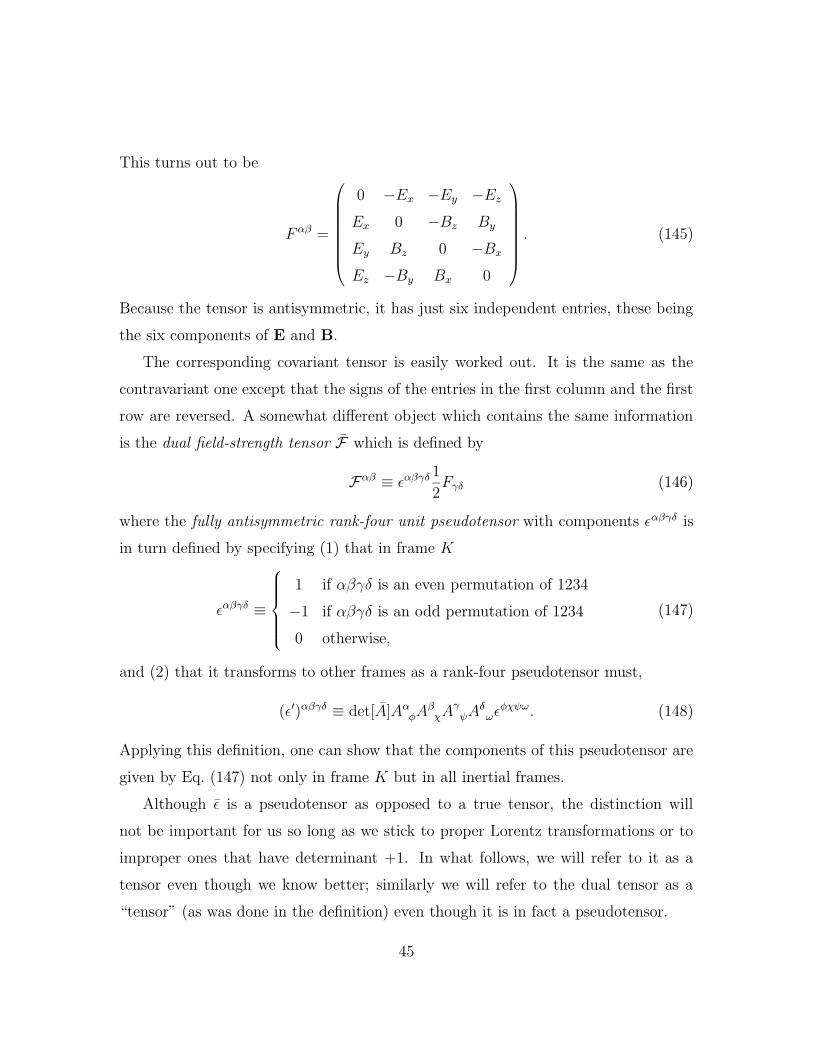
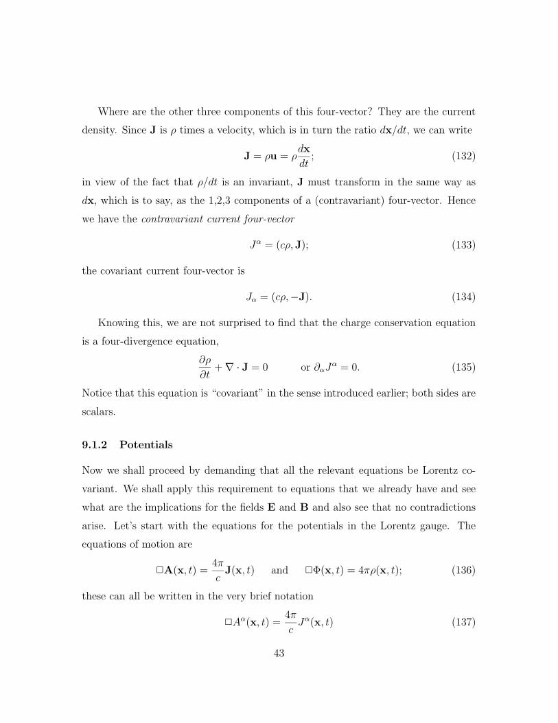
This turns out to be

F αβ =

0 −Ex −Ey −EzEx 0 −Bz By

Ey Bz 0 −Bx

Ez −By Bx 0

. (145)

Because the tensor is antisymmetric, it has just six independent entries, these being

the six components of E and B.

The corresponding covariant tensor is easily worked out. It is the same as the

contravariant one except that the signs of the entries in the first column and the first

row are reversed. A somewhat different object which contains the same information

is the dual field-strength tensor F which is defined by

Fαβ ≡ εαβγδ1

2Fγδ (146)

where the fully antisymmetric rank-four unit pseudotensor with components εαβγδ is

in turn defined by specifying (1) that in frame K

εαβγδ ≡

1 if αβγδ is an even permutation of 1234

−1 if αβγδ is an odd permutation of 1234

0 otherwise,

(147)

and (2) that it transforms to other frames as a rank-four pseudotensor must,

(ε′)αβγδ ≡ det[A]AαφAβχA

γψA

δωεφχψω. (148)

Applying this definition, one can show that the components of this pseudotensor are

given by Eq. (147) not only in frame K but in all inertial frames.

Although ε is a pseudotensor as opposed to a true tensor, the distinction will

not be important for us so long as we stick to proper Lorentz transformations or to

improper ones that have determinant +1. In what follows, we will refer to it as a

tensor even though we know better; similarly we will refer to the dual tensor as a

“tensor” (as was done in the definition) even though it is in fact a pseudotensor.

45

Returning now to the original point, Fαβ is, explicitly,

Fαβ =

0 −Bx −By −Bz

Bx 0 Ez −EyBy −Ez 0 Ex

Bz Ey −Ex 0

. (149)

9.2 Invariance of Maxwell Equations

Now we know how everything transforms; it remains to be seen whether the Maxwell

equations are Lorentz covariant. The inhomogeneous equations are

∇ · E(x, t) = 4πρ(x, t) and ∇×B(x, t)− 1

c

∂E(x, t)

∂t=

4π

cJ(x, t). (150)

The first of these is∂F 10

∂x1+∂F 20

∂x2+∂F 30

∂x3=

4π

cJ0. (151)

Because F 00 ≡ 0, we may add a term ∂F 00/∂x0 to the left-hand side of this equation

and then find that it reads

∂αFα0 =

4π

cJ0. (152)

This equation is clearly the 0th component of a four-vector equation in which the

left-hand side is obtained by taking the divergence of a rank-two tensor. The other

three inhomogeneous Maxwell equations may be analyzed in similar fashion and the

four may be concisely written as

∂αFαβ =

4π

cJβ (153)

where β =0,1,2, and 3. These are manifestly Lorentz covariant.

The homogeneous Maxwell equations are

∇ ·B(x, t) = 0 and ∇× E(x, t) = −1

c

∂B(x, t)

∂t. (154)

46

The first one can be written as

∂F10

∂x1+∂F20

∂x2+∂F30

∂x3= 0, (155)

or, since F00 = 0,

∂αFα0 = 0. (156)

The others can be expressed in similar fashion, and all four are contained in the

following equation:

∂αFαβ = 0, (157)

where β =0, 1, 2, and 3. This form is clearly covariant, establishing the covariance

of Maxwell’s equations. These equations are components of a rank-one pseudotensor.

They may also be written as components of a rank-three tensor. Notice that ∇·B = 0

is, in tensor notation,∂F 31

∂x2+∂F 23

∂x1+∂F 12

∂x3= 0. (158)

The remaining three homogeneous Maxwell equations can be expressed in similar

fashion, and all four can be written as

∂αF βγ + ∂γF αβ + ∂βF γα = 0 (159)

where α, β, and γ are any three of 0,1,2,3, giving four equations. The other possible

choices of the superscripts (involving repetition of two or more values) give nothing

(They give 0=0). Hence we have succeeded in writing each of the homogeneous

Maxwell equations in the form of an element of a rank-three tensor and the Lorentz

covariant equation we have constructed simply says that this tensor is equal to zero.

10 Transformation of the electromagnetic field

The transformation properties of E and B are easily worked out by making use of

our knowledge of how a rank-two tensor must transform:

(F ′)αβ = AαγAβδF

γδ, (160)

47

or, in matrix notation,

F ′ = AF A (161)

where A is the transpose of the matrix representing A. If we pick a frame K ′ which

is moving at velocity v = cβε1, then

A =

γ −βγ 0 0

−βγ γ 0 0

0 0 1 0

0 0 0 1

≡ A. (162)

Given the field tensor from Eq. (145), we have

F A =

βγEx −γEx −Ey −EzγEx −βγEx −Bz By

γEy − βγBz −βγEy + γBz 0 −Bx

γEz + βγBy −βγEz − γBy Bx 0

(163)

and

F ′ =

0 −Ex −γEy + βγBy −γEz − βγBy

Ex 0 βγEy − γBz βγEz + γBy

γEy − βγBz −βγEy + γBz 0 −Bx

γEz + βγBy −βγEz − γBy Bx 0

. (164)

This is an antisymmetric tensor - as it should be - and we can equate individual

elements to the appropriate components of B′ and E′. One finds

B′x = Bx B′y = γ(By + βEz) B′z = γ(Bz − βEy)

E ′x = Ex E ′y = γ(Ey − βBz) E ′z = γ(Ez + βBy). (165)

By examining these relations for a bit, one can see that

E′‖ = E‖ E′⊥ = γ[E⊥ + (β ×B)]

B′‖ = B‖ B′⊥ = γ[B⊥ − (β × E)](166)

48

where the subscripts refer to components of the fields parallel or perpendicular to β.

From the transformations one may see that when E ⊥ B, it is possible to find a

frame where one of E′ and B′ (which one?) vanishes. This is achieved by picking

β ⊥ E and β ⊥ B with an appropriate magnitude. For example, if |B| > |E|, we

take

β = β(E×B)/|E||B| (167)

where β is to be such that E′⊥ = 0, or

0 = E + β ×B = E + β[(E×B)×B]/|E||B|= E− βE|B|/|E| = E(1− β|B|/|E|)

(168)

so that we find

β = |E|/|B| (169)

which is possible if B > E.

10.1 Fields Due to a Point Charge

Another example of the use of the transformations is the determination of the fields

of a charge moving at constant velocity. Suppose a charge q has velocity u = βcε1

relative to frame K. Let K ′ move at this velocity relative to K so that the charge in

at rest in the primed frame. Further, choose the coordinates so that the charge is at

x′ = 0. Then the fields in this frame are

B′(x′, t′) = 0 and E′(x′, t′) =q

r′3x′. (170)

Let us restrict attention, without loss of generality, to the z ′ = 0 plane. There, the

electric field is

E′ =q

(√x′2 + y′2)3

[x′ε1′ + y′ε2] (171)

Using the transformations of the electromagnetic field, we find that the nonvanishing

components of the fields in frame K are

Ex =qx′

(x′2 + y′2)3/2Ey =

γqy′

(x′2 + y′2)3/2(172)

49

and

Bz =γβqy′

(x′2 + y′2)3/2. (173)

In order for these expressions to be of any use, we should express the fields in terms

of t and x rather than the primed spacetime variables.

K K’

v

b

nq

z z’

x x’

ψ

y’y

r

vt

Figure 17: Charge fixed in K ′ detected by an observer at P in K.

We shall look in particular at the fields at the point x = bε2. His position translates,

via the Lorentz transformations, into K ′ as

y′ = y x′ = −γvt and z′ = 0. (174)

Using these in the expressions for E and B, we find

Ex = −γqvt/[b2 + (γvt)2]3/2

Ey = γqb/[b2 + (γvt)2]3/2

Bz = γβqb/[b2 + (γvt)2]3/2.

(175)

It is instructive to study these results. They tell us the field at a point (0,b,0)

in K when a charge q goes along the x axis with speed v, passing the origin at time

t = 0. The fields are zero at large negative times, then Ex rises and falls to zero at

t = 0 and repeats this pattern with the opposite sign at positive times. The other

two rise to a maximum value at t = 0 and then fall to zero at large positive time. The

duration in time of the pulse if of order b/γv and becomes very short if v → c because

then γ becomes arbitrarily large. The maximum field strengths are, for Ey, γq/b2,

and, for Bz, γβq/b2. Notice that for a highly relativistic particle, β → 1, Ey ≈ Bz

50

and also that the maximum pulse strength scales as γ which means it becomes very

large (but for a very short time) as the velocity approaches c.

51