the spatial ecology of coral reef fishes · common on coral reefs. however, the response of...
TRANSCRIPT
This file is part of the following reference:
Welsh, Justin Quentin (2014) The spatial ecology of coral
reef fishes. PhD thesis, James Cook University.
Access to this file is available from:
http://researchonline.jcu.edu.au/40758/
The author has certified to JCU that they have made a reasonable effort to gain
permission and acknowledge the owner of any third party copyright material
included in this document. If you believe that this is not the case, please contact
[email protected] and quote
http://researchonline.jcu.edu.au/40758/
ResearchOnline@JCU

The Spatial Ecology of Coral Reef
Fishes
Thesis submitted by
Justin Quentin Welsh Bsc (Hons) James Cook University
August 2014
for the degree of Doctor of Philosophy in Marine Biology School of Marine and Tropical Biology and
ARC Centre of Excellence for Coral Reef Studies, James Cook University, Townsville, Queensland, Australia


i
Statement of Access
I, the undersigned, author of this thesis, understand that James Cook University will make this
thesis available for the use within the University Library and, via the Australian Digital Thesis
Network, for use elsewhere.
I understand that as unpublished work a thesis has significant protection under Copyright Act
and;
I do not wish to put any further restriction on access to this thesis.
__________________________________ ___________________
Signature Date

ii
Declaration of Ethics
This research presented and reported in this thesis was conducted in compliance with the
National Health and Medical Research Council (NHMRC) Australian Code of Practice for the
Care and Use of Animals for Scientific Purposes, 7th Edition, 2004 and the Qld Animal Care
and Protection Act, 2001. The proposed research study received animal ethics approval from
the JCU Animal Ethics Committee Approval Number #A1700.
__________________________________ ___________________
Signature Date

iii
Statement of Sources
I declare that this thesis is my own work and has not been submitted in any form for another
degree or diploma at my university or other institution of tertiary education. Information
derived from the published or unpublished work of others has been acknowledged in the text
and a list of references is given.
__________________________________ ___________________
Signature Date

iv
Electronic Copy Declaration
I, the undersigned and author of this work, declare that the electronic copy of this thesis
provided to James Cook University Library is an accurate copy of the print thesis submitted,
within the limits of technology available.
__________________________________ ___________________
Signature Date

v
Statement on the Contribution of Others
This thesis includes some collaborative work with my supervisor Professor David
Bellwood (James Cook University) as well as Dr Rebecca J Fox (James Cook
University), Dr Christopher HR Goatley and Dale Webber (Vemco, Canada). While
undertaking these collaborations, I was responsible for the project concept and design,
the majority of data collection, analyses and interpretation, as well as the final synthesis
of results into a form suitable for publication. My collaborators provided intellectual
guidance, equipment, financial support, technical instruction, statistical advice and
editorial assistance. Data for chapter 4 was derived from previously unpublished data
collected by Prof. David Bellwood, however, I was responsible for the data analysis,
interpretation and final synthesis of the results into a form suitable for publication.
Financial support for the project was provided by the Australian Museum and
Lizard Island Reef Research Foundation, the James Cook University Graduate Research
Scheme and the Australian Research Council Centre of Excellence for Coral Reef
Studies. Stipend support was provided by a James Cook University International
Research Scholarship. Financial support for conference travel was provided by the
Australian Research Council Centre of Excellence for Coral Reef Studies.

vi
Acknowledgements
I would like to start by acknowledge my supervisor, Professor David Bellwood.
Throughout my career as a researcher you have been an unwavering source of
encouragement, guidance and support. Words cannot express my gratitude to you for
everything you have done for me.
Furthermore, I would like to extend a special thanks to all my collaborators;
Christopher Goatley, Kirsty Nash, Dale Webber, Rebecca Fox and Roberta Bonaldo.
All of you have been an inspiration to me throughout my candidature and I will forever
appreciative for your support, advice and patience.
As with any project involving fieldwork, this would not have been possible
without the tireless efforts of many field assistants. Thank you to Roberta Bonaldo,
Yolly Bosiger, Simon Brandl, David Duchene, Christopher Goatley, Sophie Gordon,
Jess Hopf, Simon Hunt, Michael Kramer, Susannah Leahy, Carine Lefèvre, Oona
Lonnstedt, Mat Mitchell, Chiara Pisapia, Chris Pickens, Justin Rizarri, Derek Sun, Tara
Stephens, John Welsh and Johanna Werminghausen for your time, energy,
encouragement and friendship during countless hours of data collection. I am also very
grateful to the staff at the Lizard Island Research Station, and Orpheus Island Research
Station; Lyle Vale, Anne Hoggett, Lance and Marianne Pearce, Bob and Tanya Lamb,
Stuart and Kym Pulbrook, Kylie and Rob Eddie, Lachin and Louise Wilkins and Haley
Burgess. Your assistance and support made this project possible.
My thanks are also extended to a number of other people who were invaluable
along the way. I would like to thank; Sean Connolly, Jess Hopf, Marcus Sheaves,
Richard Rowe, Steven Swearer and Vinay Udyawer for analytical and statistical advice;
Roberta Bonaldo, Simon Brandl, Howard Choat, Christopher Goatley, Jen Hodge, Jess
Hopf, Charlotte Johansson, Zoe Loffler, Roland Muñoz, Jenn Tanner and one
anonymous reviwer for helpful discussion and comments on the text; Michelle Heupel
and Colin Simpfendorfer for their valuable insights and for providing data from
AANIMS receivers. Furthermore, I would like to extend a special thanks to all those
who worked behind the scenes to make research possible; G. Bailey and V. Pullella for
IT support, R. Abom, G. Bailey, G. Ewels, P. Osmond and J. Webb for boating, diving
and logistical support; J. Fedorniak and K. Wood for travel assistance; D. Ford and S.
Frances for a number of matters; and S. Manolis for purchasing.
vii
This research was made possible due to the generous support of many funding
bodies. A special thanks goes out to the Australia Museum and Lizard Island, who
supported this research through a Lizard Island Research Station Doctoral Fellowship.
Valuable funding was also provided by the James Cook University Internal Research
Awards and Graduate Research Scheme, as well as the Australian Research Council
through Prof. David Bellwood. Furthermore, many thanks are extended to James Cook
University who provided a Postgraduate Research Scholarship for the duration of my
candidature.
I am also very grateful to my close friends Karina, Jen, Ingrid, Jess, Charlotte, Jo,
Zoe and Derek. You were not only a source of happiness and kindness during my
candidature but also endless inspiration and encouragement. I am also extremely
thankful to the members of the Reef Fish Lab. A. Hoey, B. Fox, C. Lefèvre, C.
Johansson, C. Goatley, C. Heckathorn, M. Young, M. Kramer, J. Johansen, J. Hodge, J.
Tanner, K. Chong-Seng, K. Nash, P. Cowman, S. Brandl and Z. Loffler for all your
shared expertise and enthusiasm. A very special thank you goes out to my two families
in Australia, The Bellwoods (Dave, Orpha, Hannah and Oli) and Hunts (Alan, Kerry,
Kym, Annie, Emily and Simon). You truly have made me feel at home on the other side
of the world. To my family back in Canada, dad, mom and Jazzy, I cannot thank you
enough for your words of wisdom and kindness and most of all, for always being there
for me. It is because of you that I was able to realize my dream.
Last but definitely not least I would like to thank my partner, Simon Hunt. The
support, friendship, patience and especially love you have shown me have been my
greatest source of motivation. With you beside me, anything is possible.

viii
Abstract
Movement is a fundamental component of a species’ ecology and the study of space use
in organisms has a long-standing history as a conservation tool. Within an ecosystem,
numerous functional processes are conferred by taxa, and are essential to maintain
stable ecosystem processes. The application of functional roles is, however, bound by
the home ranges of the taxa responsible, and thus, the spatial ecology of organisms is of
great significance to ecosystem health. Coral reefs are among the most vulnerable
ecosystems to degradation and yet, the spatial ecology of key species which support
coral reef resilience remain largely unknown. In this thesis I therefore endeavoured to
quantify the spatial ecology of functionally important coral reef herbivores to further
our understanding of ecological processes.
Passive acoustic receivers are commonly used to remotely monitor animal
movements in the marine environment. The detection range and diel performance of
acoustic receivers was assessed using two parallel lines of 5 VR2W receivers spanning
125 m, deployed on the reef base and reef crest. The working detection range (distance
within which > 50% of detections are recorded) for receivers was found to be
approximately 90 m on the reef base and 60 m on the reef crest. No diel patterns in
receiver performance or detection capacities were detected. These results are in contrast
to those in non-reef environments, with coral reefs presenting a unique and challenging
environment for the use of acoustic telemetry.
Using a dense array of passive acoustic receivers, the maximum potential areas
occupied by the schooling herbivorous fish, Scarus rivulatus, was quantified over 7
months. Despite schooling, all S. rivulatus were site attached. On average, the
maximum potential home range of individuals was 24,440 m2 and ranges overlapped
extensively in individuals captured from the same school. The area shared by all
members of the same school was smaller than that of individual’s average home range,
measuring 21,652 m2. This suggests that school fidelity in this species may be low and
while favourable, schooling represents a facultative behavioural association. However,
schooling was found to have a beneficial influence on ecosystem processes, with
feeding rates in schooling S. rivulatus being double those of non-schooling individuals.
Despite adult parrotfish being largely site attached, the ontogeny of these fishes’
home range expansion is not yet known. This study therefore assessed the home range
size of three different parrotfish species at every stage of development following
ix
settlement onto the reef. With masses spanning five orders of magnitude, from the early
post-settlement stage through to adulthood, no evidence of a response to predation risk,
dietary shifts or sex change on home range expansion rates was found. Instead, a
distinct ontogenetic shift in home range expansion with sexual maturity was
documented. Juvenile parrotfishes displayed rapid home range growth until reaching
approximately 100 - 150 mm long. Thereafter, the relationship between home range and
mass broke down. This shift reflected changes in colour patterns, social status and
reproductive behaviour associated with the transition to adult stages.
The majority of herbivorous reef fishes are regarded as ‘roving herbivores’,
despite new evidence recording these taxa as being highly site attached. The extents to
which site-attached behaviour is prevalent in herbivorous reef fishes was assessed by
quantifying the movements of a largely overlooked family of functionally important
coral reef browsers, the Kyphosidae, and comparing their movements to other coral reef
herbivores. Kyphosus vaigiensis exhibited regular, large-scale (> 2 km). Each day
individual K. vaigiensis cover, on average, 2.5 km of reef (11 km maximum). A meta-
analysis of home range data from other herbivores found a consistent relationship
between home range size and body length. Only K. vaigiensis departs significantly from
the expected home-range body size relationship, with home range sizes more
comparable to large pelagic predators rather than other reef herbivores. These large-
scale movements of K. vaigiensis suggest that this species is a mobile link, providing
functional connectivity, and helping to support functional processes across habitats and
spatial scales.
Habitat degradation in the form of macroalgal outbreaks is becoming increasingly
common on coral reefs. However, the response of herbivores to algal outbreaks has
never been evaluated in a spatial context. Therefore, the spatial response of herbivorous
reef fishes was assessed with a combination of acoustic and video monitoring, to
quantify changes in the movements and abundances, respectively, of coral reef
herbivores following a simulated outbreak. An unprecedented accumulation of
functionally important herbivorous taxa was found in response to the algae. Herbivore
abundances increased by 267%, but only where algae were present. This pattern was
driven entirely by the browsing species, Naso unicornis and K. vaigiensis, which were
over 10x more abundant at the sites of simulated degradation. Resident individuals at
the site of the degradation exhibited no change in their movements. Instead, analysis of
the size classes of the responding individuals indicates that the increase in the

x
abundance of functionally important individuals occurred as large non-resident
individuals changed their movement patterns to feed on the algae.
Overall, the site attached nature of coral reef fish spatial ecology highlights a
spatial limitation to the scale of functional processes, and the vulnerability of reefs to
localized impacts. Indeed, the movements of the most mobile known herbivore, K.
vaigiensis, while extensive, were restricted to a single island, despite distances of only
250 m between islands. This suggests that functional connectivity provided by mobile
adults may be limited, and that processes occurring within-reefs are highly important.
Even resident taxa may be unwilling to shift their spatial patterns to consume algal
outbreaks, leaving reefs vulnerable to a patchwork of algal establishment. Such fixed
spatial patterns in coral reef fish emphasize the importance of large mobile taxa.
However, these larger individuals are often the most highly targeted by extractive
activities and can easily move beyond the boundaries of marine protected areas
(MPAs). Therefore, to protected highly important individuals, management initiatives
are required beyond small-scale reserves. Species specific management may be
required.

xi
Table of Contents Page
Statement of Access i
Declaration of Ethics ii
Statement of Sources iii
Electronic Copy Declaration iv
Statement on the Contribution of Others v
Acknowledgements vi
Abstract viii
Table of Contents xi
List of Figures xiii
List of Tables xvii
Chapter 1: General Introduction 1
Chapter 2: Performance of remote acoustic receivers within a coral reef habitat:
implications for array design 9
2.1. Introduction 9
2.2. Materials and Methods 11
2.3 Results 19
2.4 Discussion 25
Chapter 3: How far do schools of roving herbivores rove? A case study using
Scarus rivulatus 32
3.1 Introduction 32
3.2 Materials and Methods 35
3.3 Results 42
3.4 Discussion 50
Chapter 4: The ontogeny of home ranges: evidence from coral reef fishes 59
4.1 Introduction 59
xii
4.2 Materials and Methods 61
4.3 Results 65
4.4 Discussion 68
Chapter 5: Herbivorous fishes, ecosystem function and mobile links on coral reefs
75
5.1 Introduction 75
5.2 Materials and Methods 78
5.3 Results 83
5.4 Discussion 88
Chapter 6: Local degradation triggers a large-scale response on coral reefs 95
6.1 Introduction 95
6.2 Materials and Methods 98
6.3 Results 105
6.4 Discussion 112
Chapter 7: Concluding Discussion 118
References 123
Appendix A: Supplementary Materials for Chapter 2 150
Appendix B: Supplementary Materials for Chapter 4 151
Appendix C: Supplementary Materials for Chapter 5 155
Appendix D: Supplementary Materials for Chapter 6 163
Appendix E: Assessment of the impact of acoustic tagging on fish mortality and
behaviour 172
Appendix F: Publications arising from thesis 175

xiii
List of Figures Page
Fig. 1.1 Number of studies evaluating the home range size in reef fishes using visual
estimations, acoustic telemetry (active and passive combined) and other methods
(Modified from Nash et al. in review). 4
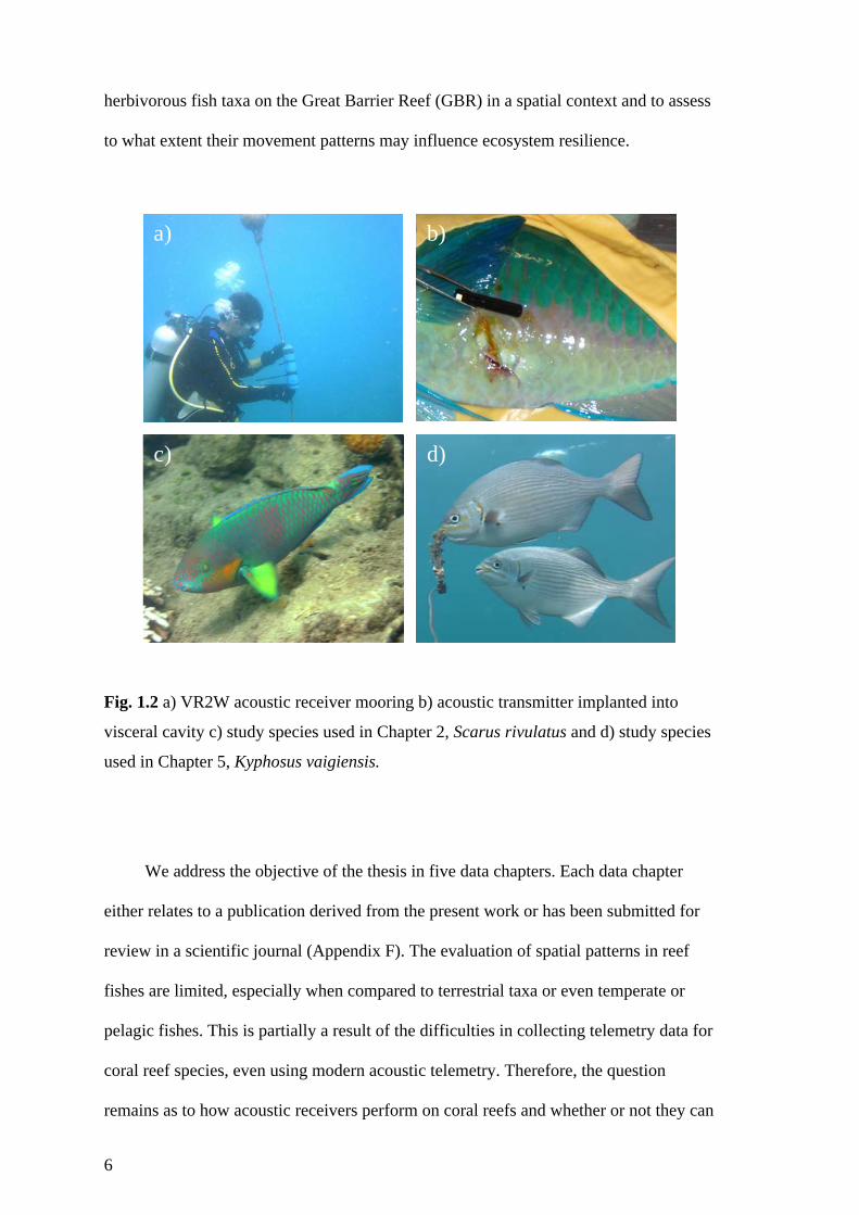
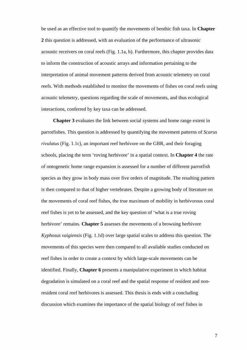
Fig. 1.2 a) VR2W acoustic receiver mooring b) acoustic transmitter implanted into
visceral cavity c) study species used in Chapter 2, Scarus rivulatus and d) study
species used in Chapter 5, Kyphosus vaigiensis. 6
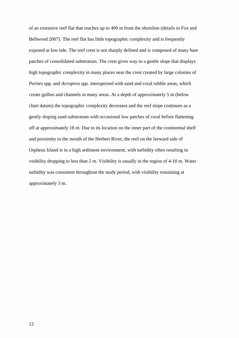
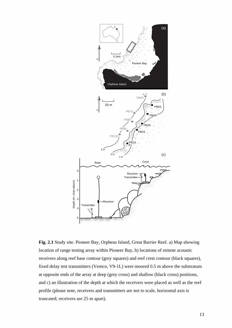
Fig. 2.1 Study site. Pioneer Bay, Orpheus Island, Great Barrier Reef. a) Map showing
location of range testing array within Pioneer Bay, b) locations of remote
acoustic receivers along reef base contour (grey squares) and reef crest contour
(black squares), fixed delay test transmitters (Vemco, V9-1L) were moored 0.5
m above the substratum at opposite ends of the array at deep (grey cross) and
shallow (black cross) positions, and c) an illustration of the depth at which the
receivers were placed as well as the reef profile (please note, receivers and
transmitters are not to scale, horizontal axis is truncated; receivers are 25 m
apart). 13
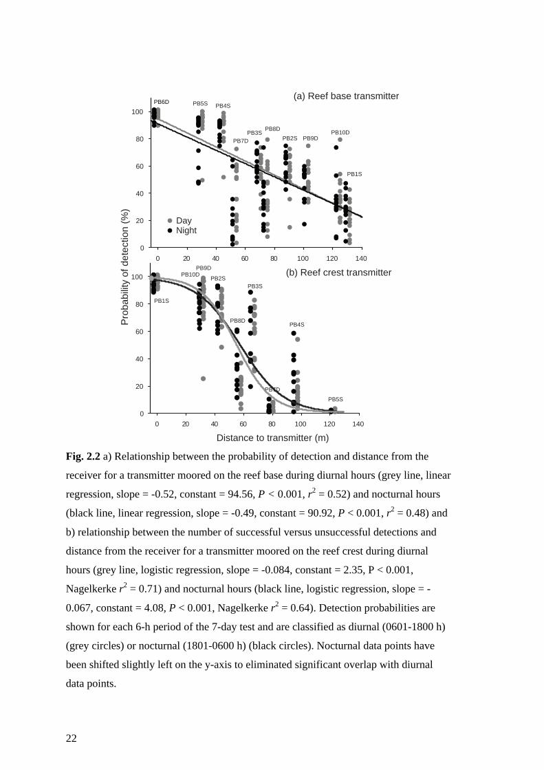
Fig. 2.2 a) Relationship between the probability of detection and distance from the
receiver for a transmitter moored on the reef base during diurnal hours (grey
line, linear regression, slope = -0.52, constant = 94.56, P < 0.001, r2 = 0.52) and
nocturnal hours (black line, linear regression, slope = -0.49, constant = 90.92, P
< 0.001, r2 = 0.48) and b) relationship between the number of successful versus
unsuccessful detections and distance from the receiver for a transmitter moored
on the reef crest during diurnal hours (grey line, logistic regression, slope = -
0.084, constant = 2.35, P < 0.001, Nagelkerke r2 = 0.71) and nocturnal hours
(black line, logistic regression, slope = -0.067, constant = 4.08, P < 0.001,
Nagelkerke r2 = 0.64). Detection probabilities are shown for each 6-h period of
the 7-day test and are classified as diurnal (0601-1800 h) (grey circles) or
nocturnal (1801-0600 h) (black circles). Nocturnal data points have been shifted
slightly left on the y-axis to eliminated significant overlap with diurnal data
points. 22
xiv
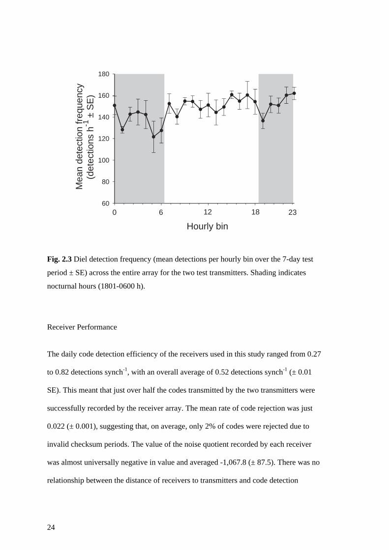
Fig. 2.3 Diel detection frequency (mean detections per hourly bin over the 7-day test
period ± SE) across the entire array for the two test transmitters. Shading
indicates nocturnal hours (1801-0600 h). 24
Fig. 3.1 Map of the placement of acoustic receivers (VR2W) within Pioneer Bay on
Orpheus Island, Great Barrier Reef. Dark grey boxes represent the placement of
shallow water receivers on the sub-tidal reef crest, and light grey boxes
represent deep water receivers moored on the reef base. The circles around each
receiver represent the receiver’s estimated detection range. 37
Fig. 3.2 Plot representing the relative proportion of total diurnal detections for each
individual Scarus rivulatus at each receiver for individuals in a) school 1, c)
school 2 and e) school 3. The diameter of each circle is in proportion to the
number of detections at a receiver. Circles provided in the legend box are
examples only. Receiver numbers in black represent reef crest receivers and
those in bold represent receivers on the reef base. The maximum area of reef
occupied by b) school 1, d) school 2 and f) school 3 within Pioneer Bay are
represented by grey areas. The solid black line represents the reef crest and the
site of capture and release of the school is represented by the black dot. Only
receivers with > 5% of individuals or schools detections are shown. 44
Fig. 3.3 Frequency histogram of the average school size that individual Scarus rivulatus
were associated with over a 5-min observational period (n = 60). The dashed
line approximates the school size frequencies that are expected following a
Poisson distribution. 47
Fig. 3.4 Feeding rate (bites min-1; mean ± SE) of a) Scarus rivulatus and b) other
scarids (which include S. ghobban, S. Schlegeli, S. niger, S. flavipectoralis and
Hipposcarus longiceps) recorded for both schooling and solitary individuals at
four discrete periods of the day at Pioneer Bay, Orpheus Island, Great Barrier
Reef. 48
Fig. 3.5 Conceptual model of the degradation in the feeding rate of schooling
individuals as individuals’ density declines and areas of home range overlap
decrease relative to non-schooling individuals, based on a doubling of feeding
rates in schools. Home range overlap was created using the random allocation of
five home ranges to a fixed area. 57
xv
Fig. 4.1 Relationship between body mass (g) and home range size (m2) for Scarus
frenatus, S. niger and Chlorurus sordidus. Triangles represent juvenile
individuals and squares and circles represent initial phase and terminal phase
individuals respectively. Grey triangles indicate juveniles, which are
predominantly omnivores/carnivores (following Bellwood 1988). The dotted
vertical line indicates the maximum body mass achieved before S. frenatus and
S. niger undergo juvenile to adult colour changes, and C. sordidus shifts from
solitary to schooling behaviour. 66
Fig. 4.2 Scale-independent relationship between body mass and home range size. To
remove the effects of scale, body mass was cube-root transformed and home
range areas were square-root transformed. Data are presented for all species;
Scarus frenatus, S. niger and Chlorurus sordidus, with the dotted line
representing the size at maturity. The fitted line is a logarithmic regression, see
text for details. 67
Fig. 5.1 Orpheus Island receiver (VR2W, Vemco) deployment sites. Black circles mark
the location of each receiver. Filled in circles represent receivers with > 5% of at
least one individual Kyphosus vaigiensis’ detections; open circles had no
significant detections. a) Map of Australia showing the location of Orpheus
Island along the Queensland coast. b) Array in Pioneer Bay showing depth
contours and numbered stars representing capture and release sites of individuals
(capture site 1: K40, K41, K42, K43, K44; capture site 2: K31, K32, K35;
capture site 3: K36, K37, K38, K39; capture site 4: K33, K34). Dotted lines
represent reef area. 80
Fig. 5.2 Relationship between home range length (m) and fish body length (√fork
length; mm) for carnivorous and herbivorous taxa with 95% confidence intervals
for each trendline. Species with a Cook’s distance value of > 0.5 are labelled
and have solid circles. 87
Fig. 6.1 Visual representation of the simulated macroalgal outbreak depicting initial
macroalgal deployment density with acoustic receiver placement. 98
Fig. 6.2 The average abundance of a) total herbivore community and b) browsing
herbivore community before (white), during (black) and after (grey) a simulated
phase shift to macroalgae. 107
xvi
Fig. 6.3 Size frequency distribution of key browsing taxa; Kyphosus vaigiensis, Naso
unicornis, K. cinerascens and Siganus doliatus before (white), during (black)
and following (grey) a simulated phase shift to macroalgae. 108
Fig. 6.4 Non-metric multidimensional scaling (nMDS) analysis showing the
relationship between 8 sites at three different treatment levels (pre, during and
post algal treatment) based on the abundance of herbivorous fish taxa. During
algal deployment, sites are designated as either control or treatment. Ellipses
represent significant groupings identified by ANOSIM. Vector lengths indicate
the relative contribution of each species to the observed pattern. Grey triangles
() represent control sites while algae were present, inverted black triangles ()
represent treatment sites while algae were present, unfilled triangles () represent
all sites prior to algal treatment and black triangles () represent all sites post-
algal treatment. 2D stress: 0.18. 110
Fig. 6.5 Change in individual detections rates (# detections.day-1 during algal
deployment - detections.day-1 prior to deployment) for all Signaus vulpinus (n =
6), S. corallinus (n = 6), Scarus schlegeli (n = 17) and Naso unicornis (n = 3).
Dark grey boxes represent fishes with core areas of detection was at the algal
deployment site (n = 4, 6, 9 and 3 respectively). Box represents mean ± SE and
whiskers represent minimum and maximum values. None of the species’ change
in detection rates following algal deployment were significantly different from
zero. 111

xvii
List of Tables Page
Table 3.1 Summary of detection data and characteristics from 18 tagged Scarus
rivulatus from three separate schools captured in Pioneer Bay, Orpheus Island,
Australia. 45
Table 3.2 Three-way ANOVA comparing the a) rank-transformed feeding rates
for Scarus rivulatus, b) pooled log-transformed feeding rates for Scarus
ghobban, Scarus schegeli, Scarus niger, Scarus flavipectoralis and
Hipposcarus longiceps 49
Table 5.1 Average metrics of Kyphosus vaigiensis movement data separated by
diurnal and nocturnal sampling periods. For individual data, please see
Appendix C. 84

1
Chapter 1: General Introduction
Habitat modification and degradation is occurring at an unprecedented global scale,
with numerous ecological repercussions (Pandolfi et al. 2003; Hoegh-Guldberg et al.
2007; Reyer et al. 2013). The human population is expected to reach 9.3 billion by 2050
(Lee 2011) and thus, an increase in the environmental disturbances caused by
anthropogenic activity is inevitable (Hughes 1994; Bellwood et al. 2012; Cinner et al.
2012). Acting in concert with direct stressors, indirect impacts such as global climate
change are predicted to lead to disturbance events, such as hurricanes and cyclones, of
increased severity, furthering the likelihood of ecosystem degradation (Hoegh-Guldberg
et al. 2007; Bell et al. 2013; Holland and Bruyère 2013). The capacity of an
environment to absorb the effects of deleterious events, and return to a healthy, pre-
disturbance state is described as that environment’s resilience (Hughes et al. 2003,
2005; Dudgeon et al. 2010). However, the resilience of the environment is largely
contingent on several factors that can undermine or support it.
Chronic pressures are among the most significant contributors to reduced
resilience (Nyström et al. 2008; Hughes et al. 2010). Examples of chronic
environmental disturbances include introduced species (Vitousek et al. 1997), nutrient
loading and eutrophication (Smith and Schindler 2009) and overexploitation of natural
populations (Lokrantz et al. 2010). Probably the best example of the effects of multiple
chronic pressures on coral reefs has been reported from the Caribbean. Overfishing
reduced the resilience of Caribbean coral reefs by significantly reducing piscine
herbivore populations, reducing ecological redundancies (Jackson et al. 2001;
Knowlton 2001; Hughes et al. 2003). As a result, the environment was unable to
recover to a pre-disturbance state following the regional scale loss of Diadema
2
antillarum and a range of other local stresses. This produced a large-scale phase-shift
that occurred on Jamaican reefs (Hughes et al. 1994). This phase-shift resulted in the
reef community shifting away from a coral dominated state, to one in which macroalgae
covered the majority of the benthos (Hughes et al. 1994; Connell 1997). Since then,
experimental studies have been able to simulate a similar effect on other tropical reefs
by excluding key species and simulating a scenario where a system’s resilience has
been undermined (e.g. Stephenson and Searles 1960; Hughes et al. 2007; Burkepile and
Hay 2010). Thus, we know how declines in coral reef health are triggered. The
challenge now is to prevent ecosystem decline by identifying and managing ecological
processes that support ecosystem resilience.
Among the key elements in ecosystem resilience are the interactions between taxa
and their environments (Bellwood et al. 2004; Elmqvist et al. 2010). Ecosystems are
reliant on a variety of functions provided by several taxa, which maintain the
environment in a normal, healthy state (Bellwood et al. 2004; Carpenter et al. 2006;
Olds et al. 2012). Examples of such functions include predation, essential for
maintaining stable, diverse populations (Terborgh et al. 2001; Knight et al. 2005);
detritivory, facilitating nutrient cycling (Depczynski and Bellwood 2003); and
herbivory, which controls algal communities (Ledlie et al. 2007; Burkepile and Hay
2010). While the functions are numerous, the species responsible for each function can
be few in number and vary extensively over different spatial scales (Cheal et al. 2012).
Functional redundancy has been suggested to be an essential element of
ecological resilience, in that key functional roles can be fulfilled by various species,
providing insurance for ecosystem functions (Sundstrom et al. 2012). However, recent
evidence suggests that functional redundancy is not as prevalent as previously assumed
(Bellwood et al. 2006; Brandl and Bellwood 2013; Johansson et al. 2013). Due to the
fine-scale niche partitioning that can exist in complex biological systems (a
3
characteristic of the tropics), there are often limited numbers of taxa capable of
conferring essential ecosystem services (Connell 1997; Patterson et al. 2003; Fox and
Bellwood 2013; Mouillot et al. 2013). Coral reefs are among the best examples, with
herbivorous coral reef fish being among the most important for reef resilience (e.g.
Hughes et al 2007). Within the herbivores, several contrasting functions exist and each
is dominated by a limited number of taxa (Bellwood et al. 2004; Burkepile and Hay
2008; Hoey and Bellwood 2009). Furthermore, when assessed using bioassays and
manipulative experiments, the rates at which the functional processes are applied and
the primary species driving them are highly variable at a range of spatial scales (Bennett
and Bellwood 2011; Vergés et al. 2011; Johansson et al. 2013).
The spatial scales over which functions are applied, is inherently bound by the
home ranges of those that moderate the process. In this sense, a great deal of the
observed variability in functional processes on coral reefs may result from the spatial
biology of key taxa (Fox and Bellwood 2011; Welsh and Bellwood 2012a).
Traditionally, the home ranges of animals have been assessed to estimate the
effectiveness of protected areas (e.g. Meyer and Holland 2005; Afonso et al. 2009;
Bryars et al. 2012), or nature reserves (e.g. Eloff 1959; Broomhall et al. 2003), and to
understand migration pathways of charismatic or commercially important species (e.g.
Berger 2004; Hedger et al. 2008). However, few studies have considered the
importance of interactions between organisms and their environment, in the context of
home ranges (but see Cooke et al. 2004; Owen-Smith et al. 2010; Fox and Bellwood
2011; Welsh and Bellwood 2012a). It is surprising that a factor such as movement,
which is intrinsic to the application of functional process, has been largely overlooked
on coral reefs, one of the most threatened environments.
Given the logistical constraints of assessing the home ranges of fishes, spatial
studies in the marine environment have historically lagged behind their terrestrial
4
counterparts. The methods associated with quantifying movement in terrestrial systems
have evolved over time from visual observations and mapping, to radio telemetry
(Harris et al. 1990; Laver & Kelly 2008) and satellite tagging (Jouventin &
Weimerskirch 1990). In the case of marine species, especially fishes, before the late 90s
studies were largely restricted to visual observations (Kramer & Chapman 1999), due to
the limitations of working in the marine environment (but see Holland et al. 1996;
Zeller 1997). However the application and refinement of acoustic telemetry in the last
few decades has made it possible to accurately monitor the movement of marine species
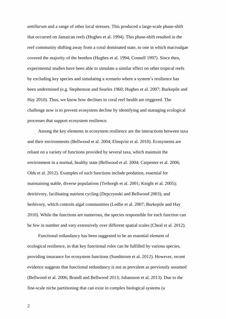
and to estimate the home range of a broader range of taxa (Fig.1.1; Bolden 2001;
Voegeli et al. 2001; Cooke et al. 2004; Heupel et al. 2006).
Fig. 1.1 Number of studies evaluating the home range size in reef fishes using visual
estimations, acoustic telemetry (active and passive combined) and other methods
(Modified from Nash et al. in review).
0
10
20
30
40
1984−1993
1994−2003
2004−2013
Num
ber o
f stu
dies Visual
Telemetry Other
5
The evolution of acoustic telemetry as a means to monitor the movement of
marine taxa has largely evolved in two directions; active and passive acoustic
monitoring. Active acoustic monitoring is used to collect high-resolution data on the
short-term movements of a focal individual (Meyer and Holland 2005; Fox and
Bellwood 2011; Welsh and Bellwood 2012a). While this technique is useful for studies
that require highly detailed data on animal movements, it is limited in that the battery
life of the transmitters is often less than a month, data collection is labour intensive
(Voegeli et al. 2001) and tracking fish from motorized vessels in shallow water may
modify their behavior (Meyer and Holland 2005; Welsh and Bellwood 2012a). For
long-term studies, passive acoustic monitoring is often favoured. Using passive acoustic
monitoring, the presence or absence data of many tagged individuals can be collected
by a network of acoustic receivers for a period of months to years (Fig. 1.2a, b; Heupel
et al. 2006; Welsh et al. 2012). Another benefit of this technology is that movements
can be tracked over large spatial scales with minimal upkeep and maintenance of the
receivers (Heupel et al. 2008). Therefore, data can be continuously collected, even in
remote location when continued access to field sites may not be permitted. With the
development of these tracking techniques for the marine environment, the study of coral
reef fish spatial biology has represented a burgeoning field of research. However, the
application of animal movement data to ecological questions has been limited and thus,
our understanding of the ecological implications of reef fish movement remain in its
infancy.
The aim of this thesis, therefore, is to provide a spatial context for ecological
interactions and to evaluate for the importance of spatial biology in ecological research.
More specifically, the studies herein are aimed to place the ecosystem functions of key
6
herbivorous fish taxa on the Great Barrier Reef (GBR) in a spatial context and to assess
to what extent their movement patterns may influence ecosystem resilience.
Fig. 1.2 a) VR2W acoustic receiver mooring b) acoustic transmitter implanted into
visceral cavity c) study species used in Chapter 2, Scarus rivulatus and d) study species
used in Chapter 5, Kyphosus vaigiensis.
We address the objective of the thesis in five data chapters. Each data chapter
either relates to a publication derived from the present work or has been submitted for
review in a scientific journal (Appendix F). The evaluation of spatial patterns in reef
fishes are limited, especially when compared to terrestrial taxa or even temperate or
pelagic fishes. This is partially a result of the difficulties in collecting telemetry data for
coral reef species, even using modern acoustic telemetry. Therefore, the question
remains as to how acoustic receivers perform on coral reefs and whether or not they can
a) b)
c) d)
7
be used as an effective tool to quantify the movements of benthic fish taxa. In Chapter
2 this question is addressed, with an evaluation of the performance of ultrasonic
acoustic receivers on coral reefs (Fig. 1.1a, b). Furthermore, this chapter provides data
to inform the construction of acoustic arrays and information pertaining to the
interpretation of animal movement patterns derived from acoustic telemetry on coral
reefs. With methods established to monitor the movements of fishes on coral reefs using
acoustic telemetry, questions regarding the scale of movements, and thus ecological
interactions, conferred by key taxa can be addressed.
Chapter 3 evaluates the link between social systems and home range extent in
parrotfishes. This question is addressed by quantifying the movement patterns of Scarus
rivulatus (Fig. 1.1c), an important reef herbivore on the GBR, and their foraging
schools, placing the term ‘roving herbivore’ in a spatial context. In Chapter 4 the rate
of ontogenetic home range expansion is assessed for a number of different parrotfish
species as they grow in body mass over five orders of magnitude. The resulting pattern
is then compared to that of higher vertebrates. Despite a growing body of literature on
the movements of coral reef fishes, the true maximum of mobility in herbivorous coral
reef fishes is yet to be assessed, and the key question of ‘what is a true roving
herbivore’ remains. Chapter 5 assesses the movements of a browsing herbivore
Kyphosus vaigiensis (Fig. 1.1d) over large spatial scales to address this question. The
movements of this species were then compared to all available studies conducted on
reef fishes in order to create a context by which large-scale movements can be
identified. Finally, Chapter 6 presents a manipulative experiment in which habitat
degradation is simulated on a coral reef and the spatial response of resident and non-
resident coral reef herbivores is assessed. This thesis is ends with a concluding
discussion which examines the importance of the spatial biology of reef fishes in

8
relation to ecosystem functioning and provides a summary of the studies available on
the movements of coral reef fishes.
9
Chapter 2: Performance of remote acoustic receivers within
a coral reef habitat: implications for array design Published in Coral Reefs 2012 31: 693-702
2.1. Introduction
Investigations of the movement patterns and site fidelity of aquatic species are now
increasingly being carried out using passive (remote) acoustic monitoring, where focal
individuals are tagged with coded transmitters and are monitored at automated listening
stations (receivers) (Afonso et al. 2009; Semmens et al. 2010; Simpfendorfer et al.
2011). Of all peer-reviewed studies carried out using remote acoustic telemetry, more
than one-third have been published in the last 3 years. Passive acoustic monitoring,
therefore, represents a burgeoning field, presenting the opportunity to track the
movement of individuals over periods of months (Egli and Babcock 2004; March et al.
2010) or years (Afonso et al. 2008; Meyer et al. 2010), and giving researchers the
opportunity to test hypotheses relating to long-term habitat usage and site fidelity. The
technology has been most frequently employed within estuarine (e.g. Hartill et al. 2003;
Heupel et al. 2006), riverine (e.g. Winter et al. 2006) or deep-water oceanic habitats
(e.g. Clements et al. 2005). Increasingly, however, the methodology is being utilized
within the coral reef environment, particularly to answer important questions relating to
the site fidelity and habitat use of harvested reef fish species (e.g. Meyer et al. 2010;
O’Toole et al. 2011).
Despite the remarkable technological advances that have facilitated the increased
ease and flexibility of use of remote acoustic monitoring, the interpretation of data
collected by automated listening stations is still a developing area of research (Lacroix
and Voegeli 2000; Clements et al. 2005; Simpfendorfer et al. 2008). Critical to the

10
interpretation of detections made by an acoustic array is an understanding of both the
detection range (Klimley et al. 1998) and the performance (sensu Simpfendorfer et al.
2008) of receivers within that array. Ultimately, the coverage yielded by the array at
any given time will determine whether the data collected represents either a minimum
or complete estimate of the animal’s movement range. Detection ranges are all too
frequently assumed, rather than tested. Where range tests are undertaken and reported
for individual studies, detection ranges can deviate from the value reported in
manufacturers’ product specifications, highlighting the discrepancy in listening range
for receivers within different aquatic habitats (Voegeli and Pincock 1996; Heupel et al.
2006). Both the detection range and performance of individual monitoring stations have
been shown to be highly variable on temporal and spatial scales (Simpfendorfer et al.
2008; Payne et al. 2010). Without a full understanding of this variability in
performance, the behaviour of the organisms being studied can be grossly
misinterpreted (e.g. Payne et al. 2010).
The constraints of the technology, and the potential for variability in the detection
performance of monitoring stations highlights the importance of properly evaluating
receiver performance prior to and during each individual study (Heupel et al. 2006).
However, there is currently a paucity of studies focusing on the acoustic equipment and
its performance, especially on coral reefs (Heupel et al. 2008). As information on
equipment performance in any given environment is integral to understanding telemetry
results, variability in detection ranges between different environments should be a
consideration in data analysis and interpretation. This is particularly important on coral
reefs, which represent a relatively new and potentially difficult environment for the
acoustic technology. Coral reefs are extremely noisy environments with a plethora of
reef noise generated by the feeding, mating and territorial displays of invertebrates and
fish taxa (e.g. Cato 1978; McCauley and Cato 2000; Simpson et al. 2008a, b). Reef
11
noise, coupled with the high topographic complexity of coral reefs, may result in a
highly variable acoustic receiver detection range, unique to the reef environment. The
synergistic effects of the aforementioned obstacles when working on coral reefs stand to
significantly affect the performance of acoustic receivers, with median detection ranges
being reported as low as 108 m with a minimum value of 55 m (Meyer et al. 2010), well
below manufacturer’s specifications.
Recently, several performance metrics such as code detection efficiency, rejection
coefficients, and noise quotients have become available, making it possible to evaluate
the performance of receivers individually. The availability of performance metrics at
the scale of the individual receiver has created the potential to better understand how
the complexity and acoustic environment of coral reefs are influencing the receiver’s
capacity to detect acoustic transmitters, ultimately leading to an ameliorated capacity to
interpret telemetry data (Simpfendorfer et al. 2008).
The goals of the current study were: first, to investigate the detection range and
performance of ultrasonic acoustic receivers within a specific shallow coral reef
environment and, second, to provide data to inform the design of listening arrays and
interpretation of animal movement patterns within coral reef habitats more generally.
The specific aims of the study were to determine (1) the effective working detection
range of 9-mm acoustic transmitters within a coral reef environment, and (2) the extent
of diel variability in acoustic receiver performance on a coral reef.
2.2. Materials and Methods
The study site was a 1.5-km stretch of fringing reef within Pioneer Bay, Orpheus Island,
a granitic island in the inner-shelf region of the Great Barrier Reef lagoon (Fig. 2.1a).
The leeward stretch of reef within Pioneer Bay is a low-energy environment composed
12
of an extensive reef flat that reaches up to 400 m from the shoreline (details in Fox and
Bellwood 2007). The reef flat has little topographic complexity and is frequently
exposed at low tide. The reef crest is not sharply defined and is composed of many bare
patches of consolidated substratum. The crest gives way to a gentle slope that displays
high topographic complexity in many places near the crest created by large colonies of
Porites spp. and Acropora spp. interspersed with sand and coral rubble areas, which
create gullies and channels in many areas. At a depth of approximately 5 m (below
chart datum) the topographic complexity decreases and the reef slope continues as a
gently sloping sand substratum with occasional low patches of coral before flattening
off at approximately 18 m. Due to its location on the inner part of the continental shelf
and proximity to the mouth of the Herbert River, the reef on the leeward side of
Orpheus Island is in a high sediment environment, with turbidity often resulting in
visibility dropping to less than 2 m. Visibility is usually in the region of 4-10 m. Water
turbidity was consistent throughout the study period, with visibility remaining at
approximately 3 m.
13
Fig. 2.1 Study site. Pioneer Bay, Orpheus Island, Great Barrier Reef. a) Map showing
location of range testing array within Pioneer Bay, b) locations of remote acoustic
receivers along reef base contour (grey squares) and reef crest contour (black squares),
fixed delay test transmitters (Vemco, V9-1L) were moored 0.5 m above the substratum
at opposite ends of the array at deep (grey cross) and shallow (black cross) positions,
and c) an illustration of the depth at which the receivers were placed as well as the reef
profile (please note, receivers and transmitters are not to scale, horizontal axis is
truncated; receivers are 25 m apart).
Pioneer Bay
0.1km
Orpheus Island
(a)
5
4
3
2
1
0
CrestBase
Transmitter
TransmitterReceiver
Receiver
1 m0 m
5 m
N
Dep
th (m
; cha
rt da
tum
)
N
PB1S
PB2S
PB3S
PB4S
PB5S
PB6D
PB7D
PB8D
PB9D
PB10D
25 m
(b)
(c)
14
Transmitter detection-range tests
Maximum detection range
Prior to the commencement of the study, preliminary tests were carried out to determine
the maximum unobstructed detection range of 9-mm acoustic transmitters using fixed
delay transmitters, which have a predictable, and constant, transmission interval
(Vemco, V9-1L, 69 kHz, 5-s repeat rate, power output 146 dB re 1 lPa at 1 m). These
data were then used to estimate effective distance increments between receivers for
temporal detection range evaluations. In these initial tests, a single remote acoustic
receiver (VR2W, Vemco. Ltd., NS, Canada) was moored at a depth of 2 m
(approximately 5 m seaward off the reef crest). A fixed delay transmitter was then
moored for approximately 15 min at a distance of 50 m from the receiver, a sufficient
amount of time for the transmitter to produce more than 100 signal transmissions. After
this time, the transmitter was moved parallel to the reef, maintaining the same depth, to
a distance of 75 m where it was moored for an additional 15 min. The procedure was
repeated at 100, 125 and 150 m fixed distances from the receiver. The detection
efficiency of the receiver at each distance was then calculated based on the number of
recorded detections divided by the number expected over the deployment period at each
distance increment. The value for the expected number of detections could be
calculated from preliminary laboratory tests of the transmitter run prior to the field
deployment, as signals were produced by the transmitter at fixed, non-random time
intervals. The transmission interval was determined to be 8 s as a result of the
approximate 3 s it takes for the transmitter to emit a complete signal pulse train coupled
with the 5-s fixed delay transmission interval, giving an expected detection rate of 7.5
signals min-1.

15
Effective detection range and temporal variation in detection
Between 25th February and 3rd March 2011, 10 VR2W acoustic receivers were
deployed in Pioneer Bay. Based on the results of preliminary tests to determine
maximum detection range within the reef habitat (see above), the receivers were
positioned in parallel lines following two distinct reef zones. Each line along the reef
consisted of 5 VR2W receivers and was configured with the first two receivers spaced
50 m apart and the remaining 3 receivers spaced at 25 m increments (i.e. 0, 50, 75, 100
and 125 m from start point respectively; Fig. 2.1b). This deployment configuration is
designed to achieve high detection area coverage to estimate various spatial attributes of
site attached fish such as their home range (e.g. Marshell et al. 2011) or the median
distance travelled (Murchie et al. 2010). One line of receivers was positioned just
shoreward of the reef crest while the other receiver line followed the reef base contour
(Fig. 2.1b). Moorings for the receivers on the reef crest were placed at a depth of
approximately 1 m (below chart datum) and consisted of a 50 cm metal pole, the base
of which was sunk into a 30 kg concrete block. Receivers were fixed to the pole and
oriented vertically upwards with the hydrophone extending 10 cm above the top of the
metal pole in order to minimise interference between the mooring structure and
hydrophone reception (Clements et al. 2005). The shallow crest receivers were
therefore about 0.5 m below chart datum. Receivers along the reef base contour were
attached to a simple rope mooring which was anchored to the sea floor at a depth of
approximately 5 m. Receivers were fixed to the rope at least 1 m below a sub-surface
float, which held the receiver vertical in the water column at a depth of about 3 m.
While the receivers were deployed, climactic conditions remained consistent, with
moderate winds (< 15 kn) and swell (< 60 cm), overcast skies and < 1 mm of rain.
16
Two coded transmitters (Vemco, V9-1L, 69 kHz, random delay interval 190-290
s, power output 146 dB re 1 µPa at 1m) were moored at opposite ends of each receiver
line, one adjacent to receiver PB1 (1 m from receiver; transmitter 1) and the other
adjacent to receiver PB6 (transmitter 2) (Fig. 2.1b, c). The transmitters were held 0.5 m
from the substratum, simulating the depth at which most medium to large (20-70 cm
TL) benthic reef fish would be active while foraging or swimming. As a result of the
long random delay interval of the transmitters used in the long-term range testing
experiment, the number of code transmissions produced cannot be calculated with the
required precision over short time periods (hours) in the same manner as a transmitter
with a fixed delay transmission interval. Therefore, the number of detections recorded
by PB1 and PB6 for transmitters 1 and 2, respectively, were used for analysis as the
number of transmissions made by each transmitter during the study period. The
transmitters were left in place for a 7 d period, after which time they were removed
from the study site and the detection data files downloaded from each VR2W receiver.
Immediately after the 7-day data collection period, the transmitters used for the long-
term deployment were assessed to determine if they were representative of typical V9
transmitters. To do this, both transmitters used in the study and an identical third
transmitter (Vemco, V9-1L, 69 kHz, random delay interval 190-290 s, power output
146 dB re 1 µPa at 1m) were moved to a mooring 50 m from a receiver, which was left
in place for a 12 h period. Following this, the receiver was collected and data was
downloaded to compare the average number of detections from each transmitter during
five randomly selected 30 min time periods.
17
Data analysis
Overall detection probabilities and effective detection range
The average number of detections from the transmitters deployed on the array, and a
third transmitter, were compared using a one-way ANOVA. The assumption of
normality was inspected using residual plots, and homogeneity of variances was
checked using Levene’s test for homogeneity of variances. No transformations were
required to meet the assumptions of ANOVA.
For each of the two test transmitters, detections recorded at individual receivers
over the 7-day test period were grouped into 6-h bins and classified as either ‘‘day’’
(0601-1800 hours) or ‘‘night’’ (1801-0600 hours). Individual detection probabilities for
each 6-h period at each receiver were calculated based on the total number of recorded
detections expressed as a percentage of the known number of transmissions (derived
from the number of detections from the receiver adjacent to the transmitter). Missed
transmissions due to signal overlap from occasional visits of tagged taxa to the study
site were factored into the analysis. Individual detection probabilities for each receiver
were then plotted against the distance from the receiver to the transmitter for diurnal
and nocturnal sampling periods. Detections were modeled using linear regressions and
logistic regressions. For the reef base, a linear regression analysis was the best model
for the data (distance to transmitter as independent variable). For the reef crest, the
relationship between number of detections (number of signals per day present vs. absent
across the array) and the distance from the transmitter was best modeled by a logistic
regression.
18
Temporal (diel) variation in detection
Temporal variation in detection probabilities were examined by calculating the average
number of detections for each of the 12-h diurnal and nocturnal sampling periods
(average values per 12-h bin were treated as individual data points for analysis).
Differences in the proportion of signals detected by each receiver in diurnal and
nocturnal sampling periods were then compared using a repeated measures analysis of
variance (RMANOVA).
To evaluate the effect of interference, which may occur on a regular diel basis
(such as reef noise), diel detection densities (hourly detection frequencies) across the
array as a whole were also examined. For each day during which the array was in place,
detections from the two test transmitters were grouped into hourly bins to give a total
number of detections hour-1 by the array. Hourly values were then averaged across the 7
days of the study to give a mean hourly detection frequency in each of the 24 hourly
bins, and these hourly detection frequencies were compared using a Chi-squared
goodness of fit test. To detect any fine-scale cyclical patterns in diel detection
frequency, a Fast Fourier Transformation (FFT) (with Hamming window smoothing)
was also applied to the data. Following Payne et al. (2010) the magnitude of variation
of each hourly bin (the standardized detection frequency or SDF) around the overall
mean daily detection frequency was then calculated as: SDFb = Bb/µ, where B is the
mean detection frequency in each of the hourly bins and l is the overall mean detection
frequency. Therefore, should acoustic interference be high at certain periods of the day,
we would expect low SDF values for the hourly bins during that time period as the
receiver would be detecting fewer than average detections. This provides an indication
of the extent to which transmitter detections may have been under-represented during
particular parts of the diel cycle due to environmental factors.
19
Acoustic performance
Parameters recorded in the metadata file downloaded from each VR2W receiver were
used to provide a quantitative metrics of the overall performance of the array. Metrics
were based around four specific parameters relating to the 8-pulse train emitted by the
coded transmitters used in this study: (1) the total number of pulses recorded each day
by a receiver (P); (2) the number of recorded detections (D); (3) the number of valid
synchs (where a synch is the interval between the first two pulses of the 8-pulse train
that identifies the incoming code as belonging to a transmitter) (S) and; (4) the number
of codes rejected due to invalid checksum periods between the final two pulses of the
train (C). From these parameters the daily code detection efficiency (D!S-1), daily
rejection coefficient (C!S-1) and daily noise quotient (P-S!# of pulses required to make a
valid code) were calculated for each receiver (see Simpfendorfer et al. 2008 for further
description of individual parameters and metrics). It is worth noting that the VR2W can
also count non-synch periods (periods generated by transmission overlap and noise
interpreted by the receiver as pings) as syncs, however, there was very little evidence of
this factor herein. The effect of the receiver’s distance from each of the moored
transmitters on the aforementioned performance metrics was evaluated using Pearson’s
correlation analysis.
2.3 Results
Maximum detection range
The preliminary tests of maximum detection range revealed a rapid decline in detection
probability for a 9 mm transmitter over short distances within the reef environment. At
50 m from the receiver only 62% of transmissions from a fixed delay range-testing
20
transmitter were detected, decreasing to a probability of just 4% at a distance of 150 m.
At a distance of 125 m from the receiver, 22% of transmissions were detected, beyond
this distance, detection values fell to below 5% and therefore, 125 m was taken to be the
maximum workable detection range within the study reef environment. This means that,
in the absence of other competing transmitters, a lone individual tagged with an
acoustic transmitter must be resident, on average, for at least 1090 s
([190 + 290]!0.22-1) to be detected at a distance of 125m.
Overall detection probabilities and detection range
For each transmitter a significant negative relationship existed between both diurnal and
nocturnal detection probabilities and distance from receiver (Fig. 2.2). The slopes and
intercepts for the regression equations for diurnal and nocturnal periods were similar on
both the reef crest (y = e4.91-0.08(x)/(1 + e4.91-0.08(x) and y = e4.75-0.07(x)/(1 + e4.91-0.08(x),
respectively) and on the base (y = 94.56-0.52x and y = 90.92-0.49x, respectively). For
the 9-mm transmitter (random delay interval transmitter) moored on the reef base (next
to the deep receiver line), detection probabilities decreased gradually at increasing
distance from the receiver (Fig. 2.2a). For practical purposes, a cut-off of 50% detection
efficiency was deemed acceptable for biological interpretation (Payne et al. 2010),
meaning that the effective working detection range for this deep transmitter was 90 m.
However, an average 30% of detections were still being recorded at a distance of 125 m
from the transmitter. For the 9-mm transmitter moored on the reef crest (next to the
shallow receiver line), detections dropped off much more steeply, driven for the most
part by the small probability of detection by receivers moored along the reef base (Fig.
2.2b). In this case, the working (50%) detection range was just 60 m (Fig. 2.2b),
although this increased to approximately 90 m when considering only detections by the

21
shallow line of receivers. In contrast to the results for the deep transmitter, virtually no
detections were being recorded at a distance of 125 m from the shallow transmitter,
even by the shallow line of receivers (Fig. 2.2b).
Differences in the number of detections from the transmitter deployed on the reef
base and the one on the reef crest cannot be attributed to differences in transmitter
performance. Post hoc tests revealed no significant difference between the numbers of
transmissions made by either of the transmitters used over the 7-day trial period or a
third transmitter used to compare transmitter performance (F2,12 = 1.27, P > 0.05).
22
Fig. 2.2 a) Relationship between the probability of detection and distance from the
receiver for a transmitter moored on the reef base during diurnal hours (grey line, linear
regression, slope = -0.52, constant = 94.56, P < 0.001, r2 = 0.52) and nocturnal hours
(black line, linear regression, slope = -0.49, constant = 90.92, P < 0.001, r2 = 0.48) and
b) relationship between the number of successful versus unsuccessful detections and
distance from the receiver for a transmitter moored on the reef crest during diurnal
hours (grey line, logistic regression, slope = -0.084, constant = 2.35, P < 0.001,
Nagelkerke r2 = 0.71) and nocturnal hours (black line, logistic regression, slope = -
0.067, constant = 4.08, P < 0.001, Nagelkerke r2 = 0.64). Detection probabilities are
shown for each 6-h period of the 7-day test and are classified as diurnal (0601-1800 h)
(grey circles) or nocturnal (1801-0600 h) (black circles). Nocturnal data points have
been shifted slightly left on the y-axis to eliminated significant overlap with diurnal
data points.
0 20 40 60 80 100 120 1400
20
40
60
80
100 (b) Reef crest transmitter
Distance to transmitter (m)
PB1S
PB2SPB3S
PB4S
PB5SPB7D
PB8D
PB9DPB10D
0 20 40 60 80 100 120 1400
20
40
60
80
100
Day Night
(a) Reef base transmitter
Prob
abilit
y of
det
ectio
n (%
)
PB1S
PB2SPB3S
PB4SPB5SPB6D
PB7D
PB8DPB9D
PB10D

23
Temporal (diel) variation in detection
The comparison of average detection probabilities for 12-h diurnal and nocturnal
periods revealed no significant diel difference in signal detection probability for the
deep receiver line (F1,8 = 0.17, P = 0.69) or the shallow receiver line (F1,8 = 0.02, P =
0.88). On an hour-by-hour basis there were some differences in detection frequencies
over the course of the day (χ222 = 34.62, P = 0.042). However, the overall diel pattern of
detection densities did not reveal any distinct trend in over- or under-representation of
detections during nocturnal or diurnal hours (Fig. 2.3). FFT analysis likewise revealed
no prominent diel cycles of detection in the observed power spectrum (please see
Appendix A for FFT output). Instead, several major peaks were found and those with
the greatest spectral density occurred at 40, 10 and 16.7 hour cycles (see Appendix A).
Standardisation of detection frequencies to remove any artefacts of environment and
varying distance to receiver on detection frequency confirmed that there was little diel
variation in detection density, with the only discernable pattern being an under-
representation of detections in the period around dawn (0500-0600 h) (Fig. 2.3).
Otherwise, both positive and negative variation around the mean daily detection
frequency was observed in both diurnal and nocturnal periods (Fig. 2.3).
24
Fig. 2.3 Diel detection frequency (mean detections per hourly bin over the 7-day test
period ± SE) across the entire array for the two test transmitters. Shading indicates
nocturnal hours (1801-0600 h).
Receiver Performance
The daily code detection efficiency of the receivers used in this study ranged from 0.27
to 0.82 detections synch-1, with an overall average of 0.52 detections synch-1 (± 0.01
SE). This meant that just over half the codes transmitted by the two transmitters were
successfully recorded by the receiver array. The mean rate of code rejection was just
0.022 (± 0.001), suggesting that, on average, only 2% of codes were rejected due to
invalid checksum periods. The value of the noise quotient recorded by each receiver
was almost universally negative in value and averaged -1,067.8 (± 87.5). There was no
relationship between the distance of receivers to transmitters and code detection
12 1860
80
100
120
140
160
180
23 6 0
Hourly bin
Mea
n de
tect
ion
frequ
ency
(det
ectio
ns h
-1 ±
SE)
25
efficiency (r = -0.20, P > 0.05), code rejection rate (r = 0.23, P > 0.05) or the noise
quotient (r = -0.16, P > 0.05).
2.4 Discussion
Our results suggest that the working detection range for 9-mm transmitters (Vemco,
V9-1L, 69 kHz, power output 146 dB re 1 µPa at 1m), the size most suited for the
majority of benthic reef fishes on coral reefs, may be as low as 60 m. While transmitters
with higher power outputs may be detectable at a slightly greater range, this value is a
fraction of the ranges previously reported in the literature for this size of transmitter
within aquatic habitats. For example, a 450-m range was reported for 9-mm transmitters
in the Caloosahatchee River (Simpfendorfer et al. 2008), and a 200-m detection range
was reported for V9-2L transmitters (with a similar power output to those used herein)
in temperate reef habitats of South Australia (Payne et al. 2010). Instead, the overall
detection range found herein is most comparable to the minimum detection range of 60
m reported by Meyer et al. (2010) on Hawaiian reefs. Our results suggest that the
detection performance of acoustic receivers may be significantly impacted by the
unique nature of the reef environment and demonstrates the importance of testing the
range of acoustic arrays across individual habitats and study sites.
In the case of Pioneer Bay, the receiver performance metrics may provide
potential explanations for the reduced detection ranges reported. The low code rejection
coefficients exhibited by receivers indicates that codes were not being rejected because
of invalid checksum values (values that check the integrity of the code transmission
used by the receiver to validate the code and confirm it is a recognisable transmitter).
The reduced detection efficiencies recorded in this study, therefore, were driven by the
receiver unit not receiving the full sequence of pulses emitted by the transmitter. For the
coral reef environment, there are several possible explanations for the reception of
26
incomplete code sequences by the receiver. These include (1) distortion of the acoustic
pulse train (e.g. dampening of amplitude) via interference from environmental noise
(acoustic waves) (both physical and biological sources and periodic or chronic); (2) the
distortion of the code sequence via reflection off topographically complex substrata; (3)
the distortion of the code sequence via absorption by particles in the water; (4) collision
with pulses from other transmitters within the detection range of the receiver; (5)
blockage of the transmission by a tagged individual moving behind an obstacle. In the
case of the current study, the latter two explanations can be eliminated by virtue of the
fact that detection performance was based on stationary transmitters operating in an
environment with minimal transmitters present. This leaves background noise,
suspended sediment and topography as likely explanations for the fact that transmitter
code sequences attenuated over shorter than expected distances in the reef environment.
In terms of background noise, it has been suggested previously that the capacity
of an acoustic receiver to detect a signal emitted by a transmitter is hindered in the
presence of large amounts of background interference, such as the noise generated by
snapping shrimp and other marine taxa (e.g. Voegeli and Pincock 1996; Clements et al.
2005; Simpfendorfer et al. 2008). Intermittent noise recorded as a ping during an actual
transmitter’s transmission can cause the receiver to reject the transmission, resulting in
the receiver ignoring the actual transmitter’s acoustic signal. Continuous noise can raise
the threshold required to detect a transmission from a transmitter resulting in a lower
detection range (with fewer pings likely to be detected). Reefs are notoriously noisy
environments and, undeniably, there is a range of noises on coral reefs, mostly
biological in origin, occurring over an extremely broad acoustic spectrum. Reef noise
has been documented to reach frequencies as high as 200 kHz, in the case of the noise
produced by snapping shrimp (Au and Banks 1998). The evidence from the negative
noise quotient values in the present study suggests that, in the reef environment, the
27
receivers are not hearing intermittent noise, which would contribute to a high noise
quotient value, but are perhaps hearing continuous noise. Continuous background noise
would cause the receivers to adjust their signal detection sensitivity to ignore consistent
background noise, which may result in the occasional signal from the transmitter being
ignored, thus contributing to a lower detection range than has been reported in other
aquatic environments.
A further manner by which ambient noise may reduce the detection capacities of
the receiver is by modifying the acoustic signal of the transmitter itself. The further the
acoustic signal from a transmitter must travel, the more likely it becomes that the signal
will collide with other noise and thus, be modified. In this sense, reef noise may cause
an incomplete pulse train to reach the receiver. Ambient noise may therefore have both
an indirect (interference with the transmitter) and direct (interference with the receiver)
effect on acoustic signal detection.
Surprisingly, the current study did not detect a significant difference between the
diurnal and nocturnal performance of acoustic receivers within the reef habitat,
something which has been reported in other environments where testing of passive
acoustic arrays has been undertaken (Payne et al. 2010). In temperate, shallow, marine
environments and estuaries, the temporal variation in activity of invertebrates such as
snapping shrimp have been suggested as the cause of these patterns in the detection
range of acoustic receivers (Heupel et al. 2004, 2006). While the source of biological
noise on reefs is highly variable, and possibly more intense at night (Bardyshev 2007),
the acoustic characteristics of the noises produced are actually quite similar in diurnal
and nocturnal periods (Leis et al. 2002). Choruses from fish schools (McCauley and
Cato 2000) and invertebrates can be heard in both diurnal and nocturnal time periods
(Radford et al. 2008). Therefore, should noise be capable of having a significant impact
on the signal transmitted from a transmitter, it is likely to be having a similar impact in

28
both nocturnal and diurnal sampling periods. Small, yet significant, declines in the
number of detects were, however, recorded at dawn and dusk. These trends may arise as
a result of an increased instance of reef noise documented to occur during these time
periods on tropical reefs from fish choruses and invertebrates (Fish 1964; Cato 1978;
Radford et al. 2008). However, the absence of a distinct peak in the spectral density of
the FFT analysis herein suggests that these patterns are non-cyclic, and may be random
noise. This is most apparent when our results are compared to the strong spectral peaks
at 24 h, and secondary peaks at 6 and 12 h, described by Payne et al. (2010) using
stationary control transmitters. Although we did not see the same degree of diel
variation in the mean detection frequency of transmitters reported from previous studies
(Payne et al. 2010), our results do suggest that, to at least some extent, background
noise is contributing to lower detection ranges and small detection probabilities.
Within the reef environment at Pioneer Bay, several physical factors are also
likely to have contributed to interference in signal detection by physically blocking the
acoustic signal. High levels of suspended matter that are characteristic of turbid inshore
reefs, such as Orpheus Island, may cause reflection of acoustic signals, interrupting
acoustic pulse trains (Voegeli and Pincock 1996 cited in Simpfendorfer et al. 2008).
Moreover, the natural topographic complexity of reefs mean that a clear line of sight
between receiver and transmitter is likely to be more frequently breached than in a
sandy or muddy-bottomed lagoonal or estuarine habitat. Even in the current study
where receivers were detecting stationary transmitters, high topographic complexity
may have an impact on detection ability. Receiver PB7D, which consistently performed
below the level expected given its distance to the two transmitters, was in close
proximity to significant benthic complexity, which is likely to have effectively and
consistently blocked the acoustic signal. This result, even on a stationary transmitter,
stresses the importance of both optimal receiver placement and assessment of the

29
detection performance of individual receivers to the design of an effective remote
monitoring array.
However, the precise causes of the strong signal attenuation are probably complex
and may have several contributing factors. Intra-environmental variability in receiver
detection capacities, both holistically and in terms of diel variation, as seen in temperate
reefs (e.g. Payne et al. 2010), highlight the need to perform detailed range tests when
utilizing acoustic telemetry to monitor movement biology. Moreover, the unique
performance of acoustic telemetry in a variety of environments emphasizes the dangers
of simply inferring detection ranges from previous studies. It is strongly recommended
that simple range tests, such as those conducted herein, be undertaken to assess
maximum detection ranges in arrays, to help avoid misinterpretation of results.
Knowledge of the study environment and careful selection of individual receiver
placement is imperative to inferring the detection range not only of individual receivers,
but also the area covered by the detection array. Similar to the reduced detection
capacity of receiver PB7D, those receivers moored on the deep line detected a lower
than expected proportion of the acoustic signals emitted from the shallow transmitter.
This is likely to be due to the fact that pulses emitted from the transmitter would need to
pass the reef slope, at which point they may reflect off the reef matrix and attenuate
before reaching the receivers. Therefore the deep line of receivers is likely to be more
useful for the detection of off-reef movements and may not be effective for detecting
within-reef movement of focal organisms. Other aquatic habitats such as rivers,
estuaries and the open ocean are not likely to contain such pronounced drop-offs and
receivers are therefore likely to exhibit a more uniform performance in all directions.
For coral reefs, however, receivers are likely to have a more biased elliptical detection
range, extending further into less complex areas. The use of multiple lines of receivers
when designing arrays for the reef environment is therefore recommended for capturing

30
the movement patterns of animals over different reef zones. In the current study, a
shallow line was found to be most effective for the detection of organisms moving over
the reef crest and flat, with the likely benefits of decreased acoustic shadow-zones out-
weighing the disadvantages of potential exposure during low tide. By virtue of the
complexity to reefs, benthic organisms’ movements through structurally complex areas
may be under-represented in the data. It appears that specific care needs to be taken
during receiver deployment to minimize the number of acoustic shadow zones in areas
of high utilization by focal tagged individuals.
The results of the present study suggest that, for reef environments, maximum
detection ranges and defined diel variability in detection range cannot be assumed.
Moreover, they highlight the importance of receiver placement for passive monitoring
studies on coral reefs. In this study both environmental and acoustic attributes of coral
reefs which are likely to cause a lower detection range of acoustic transmitters were
found to be more or less constant throughout the diel period and thus, it would not be
necessary to correct for detection variability to infer activity levels across the diurnal-
nocturnal cycle. Given the size of reef fishes, 9-mm transmitters are suitable for the
majority of larger species on coral reefs. However, we suggest that studies aiming for
complete coverage of a site inhabited by individuals tagged with 9-mm transmitters (or
any transmitter with a similar power output) will require receivers in close (less than
100 m) proximity. Moreover, gated or curtain arrays may require double lines or some
other form of redundancy in the array in order to confirm the movement of an
individual past a particular point. The farther the acoustic signal must travel over the
reef, reflecting off various substrates and colliding with any number of propagating
acoustic signals, the more likely it is that the pulse will significantly attenuate before it
reaches the receiver and not be detected. A combination of particulate matter, extreme
topographic complexity and high ambient noise levels may therefore act in concert to

31
create a reduced capacity for acoustic signals to propagate in reef habitats, compared to
other aquatic environments. By their very nature, reefs create a challenge for working
with acoustic technology, the result of which appears to be a reduction in the effective
working range of 9 mm transmitters and receivers. Overall, estimates of animal
movement in the coral reef environment as determined by passive acoustic monitoring
must be interpreted with caution. In these systems, the old maxim that the absence of
evidence does not represent evidence of absence is particularly important.
32
Chapter 3: How far do schools of roving herbivores rove? A
case study using Scarus rivulatus Published in Coral Reefs 2012 31: 991-1003
3.1 Introduction
Coral reefs worldwide are showing evidence of declining health as increased instances
of coral bleaching, disease and overharvesting are taking their toll (e.g. Scheffer et al.
2001; Gardner et al. 2003; Bellwood et al. 2004; Wilson et al. 2006, 2008). In response
to the declining health of coral reefs, ecological research is beginning to focus on coral
reef resilience to better understand the extent to which coral reefs can absorb chronic
natural and anthropogenic disturbances without degrading to alternate states, such as
macroalgal dominated reefs (Folke et al. 2004; Hughes et al. 2005; Nyström et al. 2008;
Cheal et al. 2010). Numerous studies have identified key functional groups on coral
reefs, which, through their feeding activities or other interactions with their
environment, contribute significantly to coral reef resilience (e.g. Bellwood et al. 2004;
Ferreira and Gonçalves 2006; Graham et al. 2006; Nyström et al. 2008).
Herbivory, one of the key ecological processes responsible for supporting reef
resilience, and the taxa responsible for this process have been evaluated in detail on the
GBR (e.g. Fox and Bellwood 2007; Hughes et al. 2007; Bonaldo and Bellwood 2010)
and in other tropical reefs worldwide (Hay 1981; Paddack et al. 2006; Burkepile and
Hay 2008, 2010; Alwany et al. 2009). However, two underlying trends tend to emerge
when describing herbivory on coral reefs, and the GBR in particular: 1) functional
processes are often dominated by a small number of species (albeit often different
species between geographic locations), and 2) a great deal of spatial variability exists in
the magnitude of these processes both within and among reefs (e.g. Bruggemann et al.

33
1995; Bellwood et al. 2003; Mumby 2006; Hoey and Bellwood 2008, 2010; Vergés et
al. 2011). This raises the question: at what spatial scale do these key species or critical
functional groups exert their influence, and how may this shape larger scale variation in
ecosystem function? To address this question, we focus on one key group, the
parrotfishes.
Parrotfishes stand out as important members of reef fish assemblages, regardless
of the geographical location (Bruggemann et al. 1994a; Floeter et al. 2004; Fox and
Bellwood 2007; Hoey and Bellwood 2008; Burkepile and Hay 2010). Their large size,
unique jaw morphologies and numerical abundance are all factors which result in these
taxa dominating almost every functional process with which they are involved (Hoey
and Bellwood 2008; Alwany et al. 2009; Bellwood et al. 2012). However, these species
often have highly complex social behaviours, which have been suggested to govern
their movement patterns, and potentially restrict the reef area over which they feed and
thus, the area over which they contribute to the reefs’ ecological processes (van Rooij et
al 1996; Mumby and Wabnitz 2002; Bonaldo et al. 2006).
Several parrotfish taxa have been described as being highly mobile, often moving
across large areas of reef in large schools (e.g. Robertson et al. 1976; Choat and
Bellwood 1985; Clifton 1989; Myers 1989; Lukoschek and McCormick 2000; Fox and
Bellwood 2007). These schools are likely to be socially facilitated by a single, highly
abundant school-forming species, referred to as the nuclear species, and do not operate
from the perspective of the individual (Sazima et al. 2007). They benefit members by
reducing predation risk and allow access to resources, which would otherwise be
unavailable (Robertson et al. 1976; Lukoshek and McCormick 2000). The members of
these schools are often regarded as roving herbivores and the spatial range covered by
these schools is potentially extremely large. Given that the ecosystem impact of
functionally important individuals will inevitably be constrained by their spatial range,
34
an understanding of the spatial range over which schools of herbivorous fish feed is
paramount. Yet, despite the importance of spatial range in evaluating the functional
roles of individuals, the foraging ranges of both parrotfish schools and its component
members, have yet to be evaluated.
Despite the potential for parrotfishes to exhibit large-scale movement patterns,
recent evidence suggests that the home range of parrotfish species may be quite limited
(Mumby and Wabnitz 2002; Bonaldo et al. 2006; Afonso et al. 2008; Welsh and
Bellwood 2012a). For example, Chlorurus microrhinos exhibits restricted home ranges
(< 8,000 m2), and there exists the potential for small-scale reef partitioning between
individual harems. Within an individual’s home range boundaries, the feeding patterns
of C. microrhinos have been found to be heterogeneous, with the majority of their
feeding activity concentrated in only 22% of their home range. Such site-attached
behaviour may contribute greatly to the observed variation in the spatial application of
functional processes by C. microrhinos (Welsh and Bellwood 2012a). Restricted
movement patterns by individuals from key taxa raises the possibility that their
contribution to functional processes may be confined to a small area of reef. Moreover,
these findings call into question the extent to which the term “roving herbivore” can be
applied to some herbivorous reef fish species. Although there is a widespread belief that
schooling species cover large areas of reefs (e.g. Myers 1989; Randall et al. 1997;
Nyström and Folke 2001), what constitutes ‘large’ or ‘extensive’ and how different the
spatial range of schooling species are from their haremic counterparts remains to be
determined. The general assumption, however, is that the ranges of schools will be
several times larger than haremic or territorial species. To address this issue, we
selected one of the more mobile, schooling parrotfish species to examine the extent to
which a schooling roving herbivore roves.

35
The parrotfish species Scarus rivulatus is an ecologically important herbivorous
species, especially on inshore reefs of the GBR (Fox and Bellwood 2007; Hoey and
Bellwood 2008; Cheal et al. 2012). By virtue of their numerical abundance and high
feeding rates, S. rivulatus are the dominant grazers on inshore reefs (Fox and Bellwood
2007). S. rivulatus are commonly observed forming large schools (Randall et al. 1997;
Allen et al. 2003) and are widely regarded as roving herbivores, assumed to cover large
areas of reef as they forage. However, the extent to which these “roving herbivores”
rove is almost entirely unknown, as is the nature of schooling in S. rivulatus.
The aim of the present study, therefore, is to evaluate the movement patterns of
individual S. rivulatus and their foraging schools. More specifically, we aim to: 1)
quantify the foraging range of S. rivulatus and the spatial extent and temporal duration
of foraging range overlap of school members, 2) assess the implications of schooling
behaviour on the application of their functional roles on reefs, and finally, 3) to examine
the extent to which the term “roving herbivore” can be applied to this species.
3.2 Materials and Methods
Study site
This study was conducted between February and November 2011 in Pioneer Bay on the
leeward side of Orpheus Island (18°35’S, 146°20’E), an inner-shelf granitic island in
the central GBR, Australia. Pioneer Bay contains a well-developed fringing reef with an
extensive reef flat, defined reef crest, and a gradual transition to the reef base with
several interspersed coral bommies (please see Fox and Bellwood 2007 for details). The
physical water conditions of Pioneer Bay are relatively stable with little wave action,
consistent moderate turbidity, and marked seasonal temperature fluctuations (Lefèvre
and Bellwood 2010) but no thermocline.
36
Passive acoustic monitoring
The movement patterns of tagged S. rivulatus were monitored within Pioneer Bay using
a network of 25 acoustic VR2W receivers (Vemco, Amirix Pty. Ltd., NS, Canada),
deployed in the study site using a grid configuration (Fig. 3.1; cf. Heupel et al. 2006).
Receivers were moored in two parallel lines, roughly 50 m apart, one along the reef
crest and the second along the reef base. Receivers along the crest and base were spaced
approximately 100 m and 150 m apart, respectively. Receivers were moored following
Welsh et al. (2012a) with two coats of Micron CSC ablative paint prior to deployment
following Heupel et al. (2008). Evaluations of the receiver performance in Pioneer Bay
suggest that receivers have a working detection range (range at which 50% of acoustic
signals are detected) of 60 m on the reef crest. Range testing throughout the study
period found no significant temporal variability in detection range. Data were
downloaded from the receivers approximately every two months, at which time
receivers and mooring equipment was cleared of fouling organisms. Receivers were left
in place for the duration of the study period.
Fish were tagged in late April, when a school of seven individuals were tagged,
and early July of 2011, when two more schools of five and six individuals were tagged.
To capture entire schools of S. rivulatus, the school was followed until individuals
within the school began feeding, then two-monofilament barrier nets (50 x 2 m, 35 mm
square mesh) were deployed around the school with particular care taken to exclude any
fish which were not part of the target school. Once the school had been captured, fish
were transported to the Orpheus Island Research Station and placed in a 3,300 L flow-
through tank for holding prior to surgery. Fish were then anaesthetized in a tricane
methanesulfonate (MS-222) seawater solution (0.13 gL-1) for approximately 60
seconds. Following this, the total length (TL; cm) was recorded and an ultrasonic

37
transmitter (tag; V9-1L, random delay interval 190-290 s, power output 146 dB re 1
µPa at 1m, Vemco) was inserted into the peritoneal cavity (for a detailed description of
the surgical procedure, please see Welsh and Bellwood 2012a). Fish were in captivity
for a maximum of 24 h from the time of capture to the time of release, at their
respective capture sites. Fish were released from a boat by immersion of their holding
containers and were then allowed to swim away.
Fig. 3.1 Map of the placement of acoustic receivers (VR2W) within Pioneer Bay on
Orpheus Island, Great Barrier Reef. Dark grey boxes represent the placement of shallow
water receivers on the sub-tidal reef crest, and light grey boxes represent deep water
receivers moored on the reef base. The circles around each receiver represent the
receiver’s estimated detection range.
400m
10m
0.5m
2.5m
0m
5m
1.1m0.6m
1m
0.8m
0.8m
1.3m
0.8m
0.6m
0.6m
1.1m
N
1
2 3
4
5
6
7
8
9
10
11
12
13
14
15
16
17
18
19
20
21
22
23
24
25
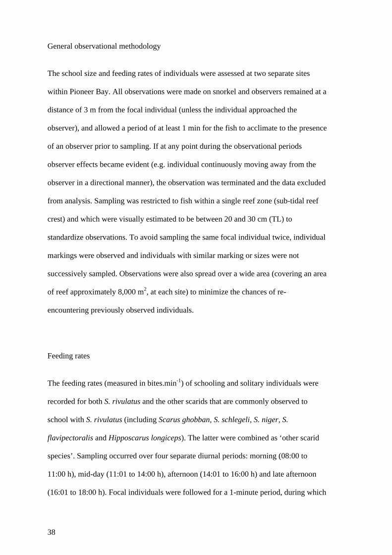
38
General observational methodology
The school size and feeding rates of individuals were assessed at two separate sites
within Pioneer Bay. All observations were made on snorkel and observers remained at a
distance of 3 m from the focal individual (unless the individual approached the
observer), and allowed a period of at least 1 min for the fish to acclimate to the presence
of an observer prior to sampling. If at any point during the observational periods
observer effects became evident (e.g. individual continuously moving away from the
observer in a directional manner), the observation was terminated and the data excluded
from analysis. Sampling was restricted to fish within a single reef zone (sub-tidal reef
crest) and which were visually estimated to be between 20 and 30 cm (TL) to
standardize observations. To avoid sampling the same focal individual twice, individual
markings were observed and individuals with similar marking or sizes were not
successively sampled. Observations were also spread over a wide area (covering an area
of reef approximately 8,000 m2, at each site) to minimize the chances of re-
encountering previously observed individuals.
Feeding rates
The feeding rates (measured in bites.min-1) of schooling and solitary individuals were
recorded for both S. rivulatus and the other scarids that are commonly observed to
school with S. rivulatus (including Scarus ghobban, S. schlegeli, S. niger, S.
flavipectoralis and Hipposcarus longiceps). The latter were combined as ‘other scarid
species’. Sampling occurred over four separate diurnal periods: morning (08:00 to
11:00 h), mid-day (11:01 to 14:00 h), afternoon (14:01 to 16:00 h) and late afternoon
(16:01 to 18:00 h). Focal individuals were followed for a 1-minute period, during which

39
time the number of bites each fish took was recorded. For each time period and each
site, a total of 10 schooling and 10 non-schooling individual S. rivulatus (and 10
schooling and 10 non-schooling other scarids) were sampled, resulting in a total of 160
observations.
School size evaluation
The school size dynamics of S. rivulatus were assessed over three discrete time periods:
morning (08:00 to 10:00 h), mid-day (12:00 to 14:00 h) and in late afternoon (15:00 to
17:00 h). During each sampling period, a single focal individual was located by the
observer and followed for 5 min. Every 30 seconds during the observation window the
number and identity of any fish species within any school with which the focal
individual became associated were counted (resulting in a total of 11 counts per
observation). A total of 10 fish per time period, per site were observed, resulting in a
total of 60 observations.
Data analysis
Individual’s site fidelity was assessed in two ways. First, a residency index (RI) was
calculated by dividing the number of days individuals were detected by the number of
possible detection days since the fish was released (which yields the percentage of days
during the monitoring period during which individuals were detected). Second, a more
detailed representation of site fidelity within Pioneer Bay was assessed by dividing the
number of diurnal detections (06:15 to 18:45 h) for each individual at each receiver by
the total number of diurnal detections for that individual. Data for each individual were
also inspected using the VUE software (Vemco) for consistent patterns of area
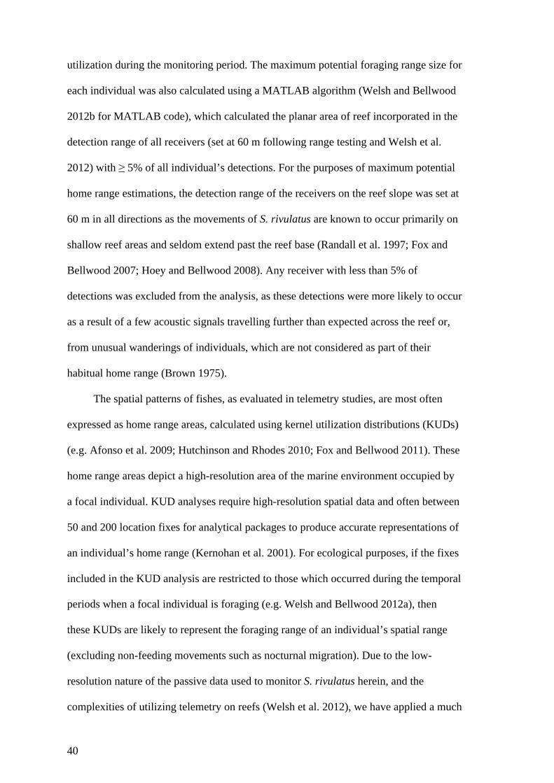
40
utilization during the monitoring period. The maximum potential foraging range size for
each individual was also calculated using a MATLAB algorithm (Welsh and Bellwood
2012b for MATLAB code), which calculated the planar area of reef incorporated in the
detection range of all receivers (set at 60 m following range testing and Welsh et al.
2012) with ≥ 5% of all individual’s detections. For the purposes of maximum potential
home range estimations, the detection range of the receivers on the reef slope was set at
60 m in all directions as the movements of S. rivulatus are known to occur primarily on
shallow reef areas and seldom extend past the reef base (Randall et al. 1997; Fox and
Bellwood 2007; Hoey and Bellwood 2008). Any receiver with less than 5% of
detections was excluded from the analysis, as these detections were more likely to occur
as a result of a few acoustic signals travelling further than expected across the reef or,
from unusual wanderings of individuals, which are not considered as part of their
habitual home range (Brown 1975).
The spatial patterns of fishes, as evaluated in telemetry studies, are most often
expressed as home range areas, calculated using kernel utilization distributions (KUDs)
(e.g. Afonso et al. 2009; Hutchinson and Rhodes 2010; Fox and Bellwood 2011). These
home range areas depict a high-resolution area of the marine environment occupied by
a focal individual. KUD analyses require high-resolution spatial data and often between
50 and 200 location fixes for analytical packages to produce accurate representations of
an individual’s home range (Kernohan et al. 2001). For ecological purposes, if the fixes
included in the KUD analysis are restricted to those which occurred during the temporal
periods when a focal individual is foraging (e.g. Welsh and Bellwood 2012a), then
these KUDs are likely to represent the foraging range of an individual’s spatial range
(excluding non-feeding movements such as nocturnal migration). Due to the low-
resolution nature of the passive data used to monitor S. rivulatus herein, and the
complexities of utilizing telemetry on reefs (Welsh et al. 2012), we have applied a much

41
more coarse estimate of spatial range. We calculated the maximum potential diurnal
foraging range by excluding nocturnal data, when fish were resting and not feeding, and
calculating the area of reef enclosed by the detection range of the acoustic receivers in
which tagged S. rivulatus were detected during the day (when they are feeding). Areas
of reef with overlapping detection ranges of two or more adjacent receivers are
excluded from the area calculation if all overlapping receivers did not detect at least 5%
of the signals from a transmitter (please see Fig. 3.2b, d, f for a representation of
maximum detection areas of each school). Therefore, this method allows for a coarse
estimation of the entire area of reef potentially occupied by an individual while foraging
(maximum foraging range) and will almost certainly be larger than the actual foraging
range.
A two-way analysis of variance (ANOVA) was used to compare the average
school size of S. rivulatus during each individual’s 5 min observation time at different
periods throughout the day and to test for a site effect. Time of day and site were fixed
factors and the average number of individuals with which the focal individual became
associated with was the dependent variable. Normality and homogeneity of variances
were assessed using residual analyses. Data were log10 transformed to improve
homogeneity of variances. School size variability was also assessed using a coefficient
of variation (CV; σ/mean), calculated for each individual during the 5 min sampling
period. The frequency distribution of the average 5 min school size with which an
individual was associated with was also compared to a Poisson distribution to test
whether the average school size differed from a random expectation (Quinn and
Keough 2002). As Poisson distributions require discrete data, average school sizes were
rounded up to the nearest integer.
The feeding rate data of the ‘other scarids’ were compared using a one-way
ANOVA. Feeding rates at different times of the day (morning, early afternoon, late
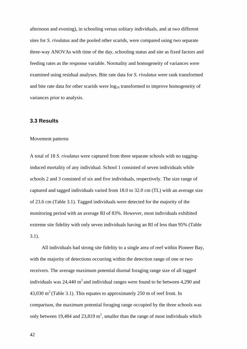
42
afternoon and evening), in schooling versus solitary individuals, and at two different
sites for S. rivulatus and the pooled other scarids, were compared using two separate
three-way ANOVAs with time of the day, schooling status and site as fixed factors and
feeding rates as the response variable. Normality and homogeneity of variances were
examined using residual analyses. Bite rate data for S. rivulatus were rank transformed
and bite rate data for other scarids were log10 transformed to improve homogeneity of
variances prior to analysis.
3.3 Results
Movement patterns
A total of 18 S. rivulatus were captured from three separate schools with no tagging-
induced mortality of any individual. School 1 consisted of seven individuals while
schools 2 and 3 consisted of six and five individuals, respectively. The size range of
captured and tagged individuals varied from 18.0 to 32.0 cm (TL) with an average size
of 23.6 cm (Table 3.1). Tagged individuals were detected for the majority of the
monitoring period with an average RI of 83%. However, most individuals exhibited
extreme site fidelity with only seven individuals having an RI of less than 95% (Table
3.1).
All individuals had strong site fidelity to a single area of reef within Pioneer Bay,
with the majority of detections occurring within the detection range of one or two
receivers. The average maximum potential diurnal foraging range size of all tagged
individuals was 24,440 m2 and individual ranges were found to be between 4,290 and
43,030 m2 (Table 3.1). This equates to approximately 250 m of reef front. In
comparison, the maximum potential foraging range occupied by the three schools was
only between 19,484 and 23,819 m2, smaller than the range of most individuals which

43
made up each school and covers an average of 219 m of reef front. The majority of
detections occurred on the reef flat and crest with those receivers detecting individuals
more often than receivers on the reef base (Fig. 3.2a, c, e). No shifts in area occupancy
were detected from the site of capture to the habitual area of reef occupied by tagged
individuals with all individuals captured from each school remaining within the same
area of the reef for the duration of the study (Fig. 3.2a, c, e). Individuals captured from
within the same school did, however, exhibit slightly different detection patterns, albeit
within the same area of reef. Individuals captured from schools 1 and 2 had a great deal
of area utilization overlap, however, areas of primary detection remained distinct
between the two schools (Fig. 3.2).
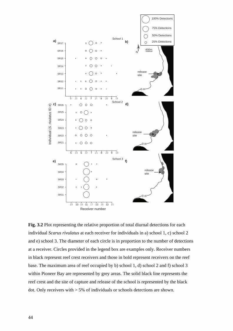
44
Fig. 3.2 Plot representing the relative proportion of total diurnal detections for each
individual Scarus rivulatus at each receiver for individuals in a) school 1, c) school 2
and e) school 3. The diameter of each circle is in proportion to the number of detections
at a receiver. Circles provided in the legend box are examples only. Receiver numbers
in black represent reef crest receivers and those in bold represent receivers on the reef
base. The maximum area of reef occupied by b) school 1, d) school 2 and f) school 3
within Pioneer Bay are represented by grey areas. The solid black line represents the
reef crest and the site of capture and release of the school is represented by the black
dot. Only receivers with > 5% of individuals or schools detections are shown.
SR31
SR32
SR33
SR34
SR35
Indi
vidu
al (S
. riv
ulat
us ID
#)
SR11
SR12
SR13
SR14
SR15
SR16
23 6 22 7 21 208 9 195
SR17
Receiver number
SR21
SR22
SR23
SR24
SR25
SR26
400mN
a) b)
23 6 22 7 21 208 9 195
19 10 18 11 17 1612 13 15
School 3
School 2
School 1
release site
release site
release site
100% Detections
75% Detections
50% Detections
25% Detections
c) d)
e) f)
0 m
0 m
0 m
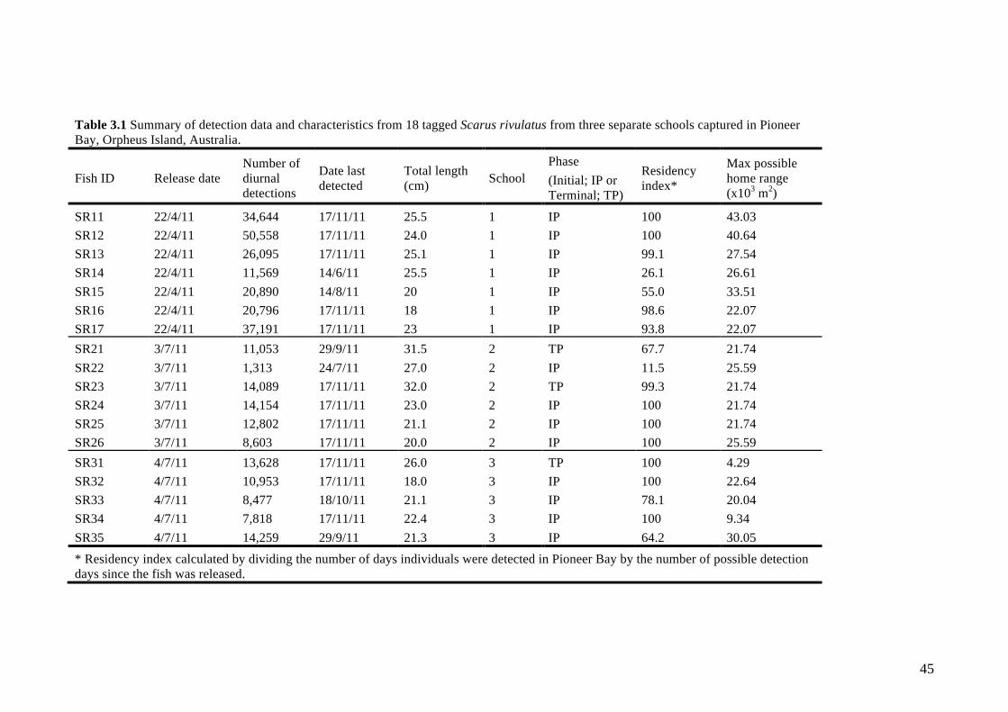
45
Table 3.1 Summary of detection data and characteristics from 18 tagged Scarus rivulatus from three separate schools captured in Pioneer Bay, Orpheus Island, Australia.
Fish ID Release date Number of diurnal detections
Date last detected
Total length (cm) School
Phase (Initial; IP or Terminal; TP)
Residency index*
Max possible home range (x103 m2)
SR11 22/4/11 34,644 17/11/11 25.5 1 IP 100 43.03 SR12 22/4/11 50,558 17/11/11 24.0 1 IP 100 40.64 SR13 22/4/11 26,095 17/11/11 25.1 1 IP 99.1 27.54 SR14 22/4/11 11,569 14/6/11 25.5 1 IP 26.1 26.61 SR15 22/4/11 20,890 14/8/11 20 1 IP 55.0 33.51 SR16 22/4/11 20,796 17/11/11 18 1 IP 98.6 22.07 SR17 22/4/11 37,191 17/11/11 23 1 IP 93.8 22.07 SR21 3/7/11 11,053 29/9/11 31.5 2 TP 67.7 21.74 SR22 3/7/11 1,313 24/7/11 27.0 2 IP 11.5 25.59 SR23 3/7/11 14,089 17/11/11 32.0 2 TP 99.3 21.74 SR24 3/7/11 14,154 17/11/11 23.0 2 IP 100 21.74 SR25 3/7/11 12,802 17/11/11 21.1 2 IP 100 21.74 SR26 3/7/11 8,603 17/11/11 20.0 2 IP 100 25.59 SR31 4/7/11 13,628 17/11/11 26.0 3 TP 100 4.29 SR32 4/7/11 10,953 17/11/11 18.0 3 IP 100 22.64 SR33 4/7/11 8,477 18/10/11 21.1 3 IP 78.1 20.04 SR34 4/7/11 7,818 17/11/11 22.4 3 IP 100 9.34 SR35 4/7/11 14,259 29/9/11 21.3 3 IP 64.2 30.05
* Residency index calculated by dividing the number of days individuals were detected in Pioneer Bay by the number of possible detection days since the fish was released.

46
School size evaluation
Schooling behaviour was extremely common for S. rivulatus. On average, individuals
were in schools for 64.8 ± 3.5% (mean ± SE, n = 60) of observations. On average, S.
rivulatus schools consisted of 5.7 ± 0.8 individuals, however, the average school size
frequency histogram was heavily skewed to the left, with the average being a great deal
larger than the mode (2.64) and median (3.54) school size (Fig. 3.3). However, average
school sizes with which an individual became associated differed significantly from
what would be expected following a Poisson distribution (χ 22 = 95.84, P < 0.001) and
thus exhibited a non-random distribution. The size of the school with which an
individual was associated was extremely variable with an average CV for each
individual over the 5 min observation period of 0.69 ± 0.04. Moreover, the frequently
observed fracturing of schools tends to suggest that little fidelity exists from the
perspective of an individual to a particular school. There was no significant difference
detected in the average school sizes of individuals throughout the day (F2,54 = 0.30, P =
0.74), nor was there any site effect (F1,54 = 3.89, P = 0.53), or interaction between site
and time period (F2,54 = 0.63, P > 0.56). Data were therefore pooled across the two sites
for graphical representation (Fig. 3.3).

47
Fig. 3.3 Frequency histogram of the average school size that individual Scarus rivulatus
were associated with over a 5-min observational period (n = 60). The dashed line
approximates the school size frequencies that are expected following a Poisson
distribution.
Feeding rates
There was no significant difference in the feeding rates of S. ghobban, S. schlegeli, S.
niger, S. flavipectoralis and Hipposcarus longiceps (F4,155 = 2.13, P = 0.08 ) and
therefore feeding data for these species were pooled as ‘other scarids’ for all analyses.
Feeding rates for both S. rivulatus and ‘other scarids’ differed significantly
throughout the day (F3,143 = 18.8, P < 0.001 and F3,145 = 9.8, P < 0.001, respectively),
with highest feeding rates detected between 14:01 and 16:00 h in both cases (Table 3.2;
Fig. 3.4). No site effects were detected for S. rivulatus or the other scarids and thus,
data were pooled across sites for presentation (Table 3.2). In both S. rivulatus and other
scarids, feeding rates were consistently and significantly higher in schooling versus
0 1 2 3 4 5 6 7 8 9 10 11 12 13 14 15 16 17 18 >19
Freq
uenc
y
0
2
4
6
8
10
12
School size (x per 5 min-1)
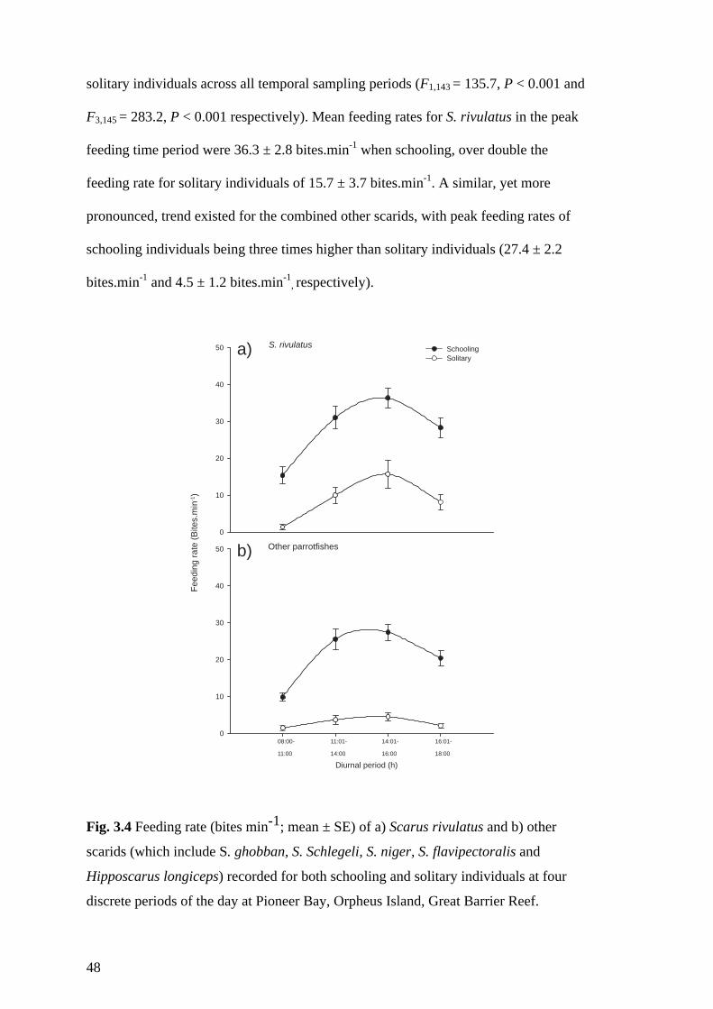
48
solitary individuals across all temporal sampling periods (F1,143 = 135.7, P < 0.001 and
F3,145 = 283.2, P < 0.001 respectively). Mean feeding rates for S. rivulatus in the peak
feeding time period were 36.3 ± 2.8 bites.min-1 when schooling, over double the
feeding rate for solitary individuals of 15.7 ± 3.7 bites.min-1. A similar, yet more
pronounced, trend existed for the combined other scarids, with peak feeding rates of
schooling individuals being three times higher than solitary individuals (27.4 ± 2.2
bites.min-1 and 4.5 ± 1.2 bites.min-1, respectively).
Fig. 3.4 Feeding rate (bites min-1; mean ± SE) of a) Scarus rivulatus and b) other
scarids (which include S. ghobban, S. Schlegeli, S. niger, S. flavipectoralis and
Hipposcarus longiceps) recorded for both schooling and solitary individuals at four
discrete periods of the day at Pioneer Bay, Orpheus Island, Great Barrier Reef.
0
10
20
30
40
50 SchoolingSolitary
Feed
ing
rate
(Bite
s.m
in-1)
0
10
20
30
40
50
08:00-
11:00
11:01-
14:00
14:01-
16:00
16:01-
18:00
Diurnal period (h)
a)
b)
S. rivulatus
Other parrotfishes
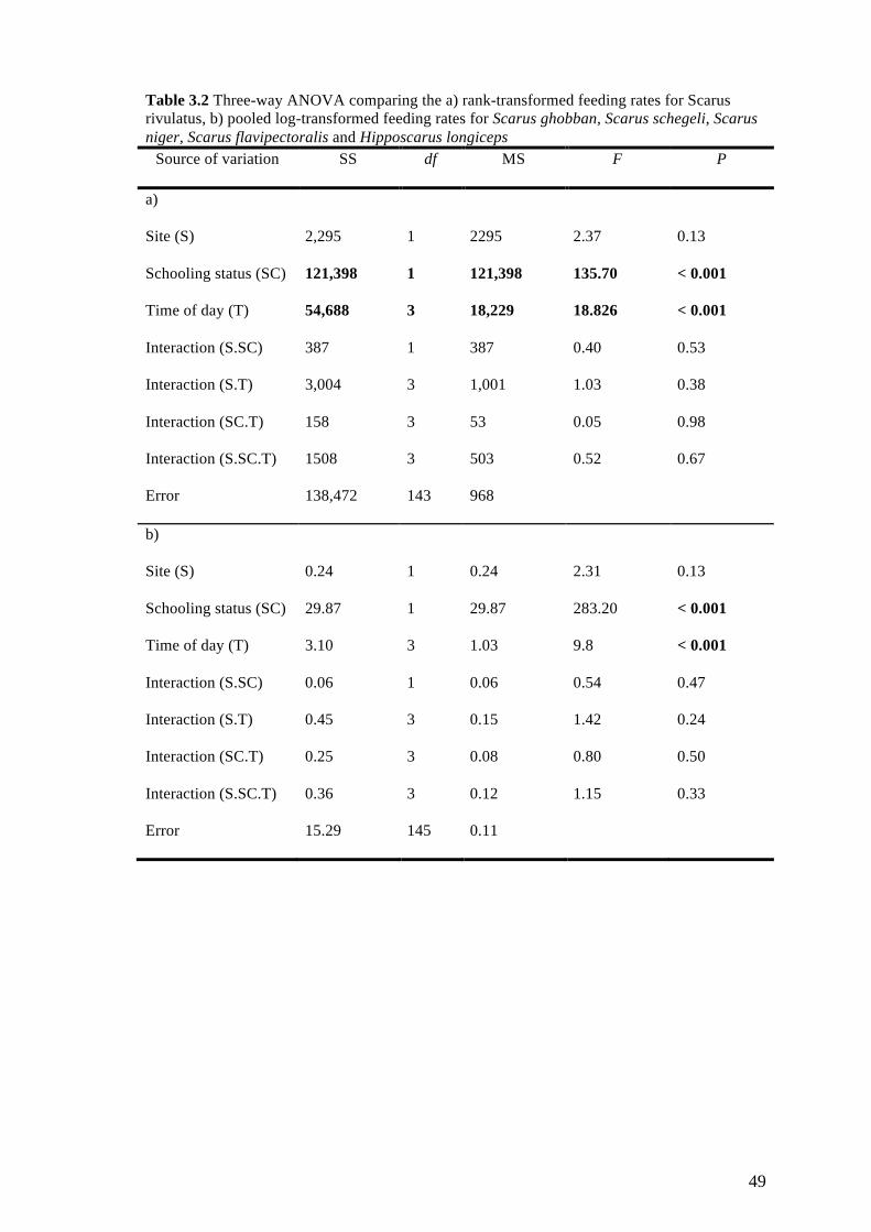
49
Table 3.2 Three-way ANOVA comparing the a) rank-transformed feeding rates for Scarus rivulatus, b) pooled log-transformed feeding rates for Scarus ghobban, Scarus schegeli, Scarus niger, Scarus flavipectoralis and Hipposcarus longiceps
Source of variation SS df MS F P
a)
Site (S) 2,295 1 2295 2.37 0.13
Schooling status (SC) 121,398 1 121,398 135.70 < 0.001
Time of day (T) 54,688 3 18,229 18.826 < 0.001
Interaction (S.SC) 387 1 387 0.40 0.53
Interaction (S.T) 3,004 3 1,001 1.03 0.38
Interaction (SC.T) 158 3 53 0.05 0.98
Interaction (S.SC.T) 1508 3 503 0.52 0.67
Error 138,472 143 968
b)
Site (S) 0.24 1 0.24 2.31 0.13
Schooling status (SC) 29.87 1 29.87 283.20 < 0.001
Time of day (T) 3.10 3 1.03 9.8 < 0.001
Interaction (S.SC) 0.06 1 0.06 0.54 0.47
Interaction (S.T) 0.45 3 0.15 1.42 0.24
Interaction (SC.T) 0.25 3 0.08 0.80 0.50
Interaction (S.SC.T) 0.36 3 0.12 1.15 0.33
Error 15.29 145 0.11

50
3.4 Discussion
Our results represent the first detailed long-term quantification of the spatial range of
school-forming individuals of a roving herbivore. The spatial range of S. rivulatus was
found to be limited, with the majority of detections for all individuals within a school
occurring within a small area, measuring on average just 24,440 m2. This suggests that
the spatial range of some nominally ‘roving’ herbivores, and the schools they form,
may actually be quite limited. The ranges are of a similar size or just 2-3 times larger
than those previously described for solitary or haremic herbivore species. Despite
general assumptions (e.g. Myers 1989), schooling did not appear to have a marked
effect of the home ranges in S. rivulatus. By combining acoustic monitoring with field
observations we found that foraging schools of S. rivulatus appear to be highly unstable
with little school fidelity. Though individuals spent most of their time within schools,
the frequent fractioning and coalescing of schools resulted in solitary individuals also
being common. The variability in school composition was supported over longer
timeframes by differing detection patterns for individuals, which were initially captured
from the same school. The overlap between the spatial ranges of individuals captured
from two distinct schools indicates that there is little exclusion of conspecifics from
within an individuals’ foraging range. The limited movement, despite schooling
behaviour, might have significant implications for the spatial application of ecosystem
functions by both the nuclear species (in this case S. rivulatus) and those species
associating with their foraging schools. Basically, this schooling, roving herbivore does
not rove very far.
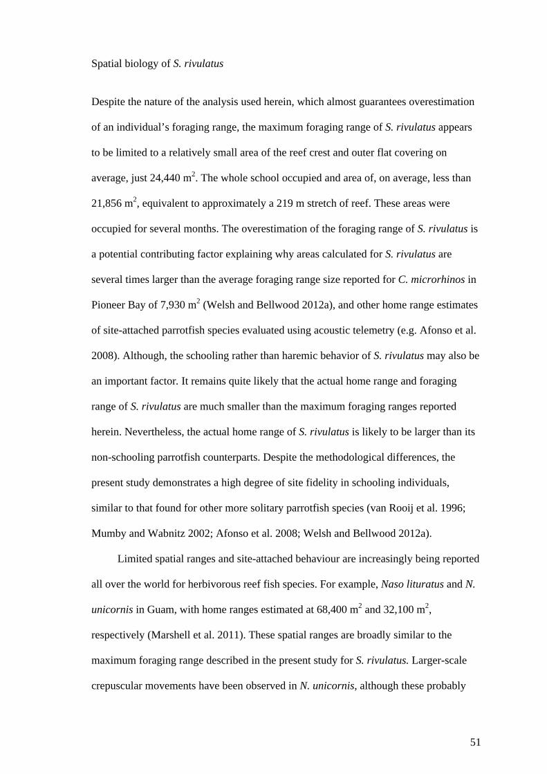
51
Spatial biology of S. rivulatus
Despite the nature of the analysis used herein, which almost guarantees overestimation
of an individual’s foraging range, the maximum foraging range of S. rivulatus appears
to be limited to a relatively small area of the reef crest and outer flat covering on
average, just 24,440 m2. The whole school occupied and area of, on average, less than
21,856 m2, equivalent to approximately a 219 m stretch of reef. These areas were
occupied for several months. The overestimation of the foraging range of S. rivulatus is
a potential contributing factor explaining why areas calculated for S. rivulatus are
several times larger than the average foraging range size reported for C. microrhinos in
Pioneer Bay of 7,930 m2 (Welsh and Bellwood 2012a), and other home range estimates
of site-attached parrotfish species evaluated using acoustic telemetry (e.g. Afonso et al.
2008). Although, the schooling rather than haremic behavior of S. rivulatus may also be
an important factor. It remains quite likely that the actual home range and foraging
range of S. rivulatus are much smaller than the maximum foraging ranges reported
herein. Nevertheless, the actual home range of S. rivulatus is likely to be larger than its
non-schooling parrotfish counterparts. Despite the methodological differences, the
present study demonstrates a high degree of site fidelity in schooling individuals,
similar to that found for other more solitary parrotfish species (van Rooij et al. 1996;
Mumby and Wabnitz 2002; Afonso et al. 2008; Welsh and Bellwood 2012a).
Limited spatial ranges and site-attached behaviour are increasingly being reported
all over the world for herbivorous reef fish species. For example, Naso lituratus and N.
unicornis in Guam, with home ranges estimated at 68,400 m2 and 32,100 m2,
respectively (Marshell et al. 2011). These spatial ranges are broadly similar to the
maximum foraging range described in the present study for S. rivulatus. Larger-scale
crepuscular movements have been observed in N. unicornis, although these probably
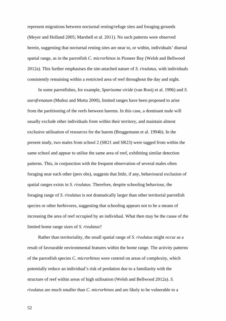
52
represent migrations between nocturnal resting/refuge sites and foraging grounds
(Meyer and Holland 2005; Marshell et al. 2011). No such patterns were observed
herein, suggesting that nocturnal resting sites are near to, or within, individuals’ diurnal
spatial range, as in the parrotfish C. microrhinos in Pioneer Bay (Welsh and Bellwood
2012a). This further emphasises the site-attached nature of S. rivulatus, with individuals
consistently remaining within a restricted area of reef throughout the day and night.
In some parrotfishes, for example, Sparisoma viride (van Rooij et al. 1996) and S.
aurofrenatum (Muñoz and Motta 2000), limited ranges have been proposed to arise
from the partitioning of the reefs between harems. In this case, a dominant male will
usually exclude other individuals from within their territory, and maintain almost
exclusive utilisation of resources for the harem (Bruggemann et al. 1994b). In the
present study, two males from school 2 (SR21 and SR23) were tagged from within the
same school and appear to utilise the same area of reef, exhibiting similar detection
patterns. This, in conjunction with the frequent observation of several males often
foraging near each other (pers obs), suggests that little, if any, behavioural exclusion of
spatial ranges exists in S. rivulatus. Therefore, despite schooling behaviour, the
foraging range of S. rivulatus is not dramatically larger than other territorial parrotfish
species or other herbivores, suggesting that schooling appears not to be a means of
increasing the area of reef occupied by an individual. What then may be the cause of the
limited home range sizes of S. rivulatus?
Rather than territoriality, the small spatial range of S. rivulatus might occur as a
result of favourable environmental features within the home range. The activity patterns
of the parrotfish species C. microrhinos were centred on areas of complexity, which
potentially reduce an individual’s risk of predation due to a familiarity with the
structure of reef within areas of high utilisation (Welsh and Bellwood 2012a). S.
rivulatus are much smaller than C. microrhinos and are likely to be vulnerable to a

53
greater number of predators, making complexity and predator avoidance potentially
more important. Therefore, the area occupied by S. rivulatus may represent an area of
familiarity, with adequate cover and known areas of escape from predators.
The nature and benefits of schooling
Small spatial ranges of individual S. rivulatus are mirrored by the entire school from
which they were captured and might be responsible, in part, for the relatively small
average school sizes of only 5.7 ± 0.83 individuals. As schools may arise from chance
encounters (Robertson et al. 1976; Lukoschek and McCormick 2000), at any one time
the number of individuals available to join a school is finite. School formation is
dependent on social interactions, the frequency of which is in turn, dependent on the
number of overlapping home ranges. As such, we would expect to see a heavily skewed
school size-frequency distribution towards smaller schools, as observed for S. rivulatus.
However, the average number of individuals with which a focal individual became
associated with over a 5-min observation period was significantly different from that of
a Poisson distribution, and was thus not effectively random. This deviation from
random occurred due to the abundance of large schooling associations suggesting that
fish actively choose to be associated with schools. Therefore, within the constraints of a
restricted home rage, schooling appears to be an ecologically favourable strategy for S.
rivulatus.
When the abundances of competitive species are high enough, territoriality, or
haremic behaviour, is suggested to no longer be favourable and schooling behaviour
may become more favourable (Bonaldo et al. 2006). To maximise their fitness, territory
holders need to trade off territory defence with mating and foraging activities (Itzkowitz
1977). It may be this trade-off, which favours the schooling behaviour, with limited

54
school fidelity, in S. rivulatus. As they are the most highly abundant Scarus species in
Pioneer Bay (Fox and Bellwood 2007; Hoey and Bellwood 2008), schooling would be
favoured over territoriality as, in this social environment, the costs of territory defense
may outweigh the benefits (Bonaldo et al. 2006) so individuals likely maximize fitness
by devoting more time to feeding and reproducing in another (non-territorial) fashion
(see Clifton 1989; Kuwamura et al. 2009). An interesting feature of the schools,
however, is that all individuals initially captured from school 1 tend to have centres of
activity, distinct from the adjacent school 2. Area partitioning of this type is similar to
that expected for territorial species as seen in C. microrhinos (Welsh and Bellwood
2012a) and S. viride (van Rooij et al. 1996). This suggests that there is little blending of
the foraging range of individuals in adjacent areas, even without any territorial
aggression, highlighting the site-attached nature of S. rivulatus. Therefore, while
schools are socially facilitated and individuals can potentially join any school operating
within their spatial range, they will not expand their home range to match the home
range of all co-schooling individuals within a school with which they are associated.
This is also supported by the average area occupied by the school being less than that of
the individuals. This occurs as the range of the school (the area where the average
percent detections of all individuals within a school are greater than 5%) is only an area
of home range overlap; and all individuals within the school do not have identical
ranges (the cumulative area of individual’s > 5% detections would be somewhat larger,
but would not be the area used by the entire school). Foraging ranges appear to be fixed
with schooling being a desirable, but facultative association.
From the perspective of an individual fish, foraging schools have been suggested
to provide several advantages, such as reduced individual predation risk, access to
resources which would otherwise be inaccessible (e.g. damselfish territories) and
increased efficiency at locating optimal foraging areas (e.g. Alevizon 1976; Robertson
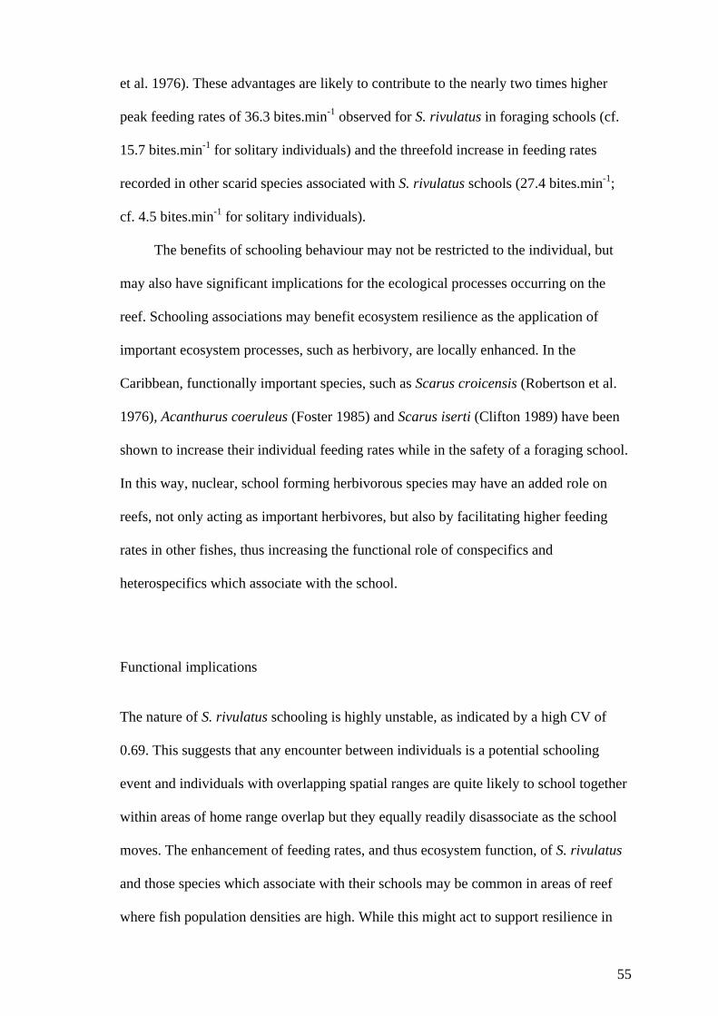
55
et al. 1976). These advantages are likely to contribute to the nearly two times higher
peak feeding rates of 36.3 bites.min-1 observed for S. rivulatus in foraging schools (cf.
15.7 bites.min-1 for solitary individuals) and the threefold increase in feeding rates
recorded in other scarid species associated with S. rivulatus schools (27.4 bites.min-1;
cf. 4.5 bites.min-1 for solitary individuals).
The benefits of schooling behaviour may not be restricted to the individual, but
may also have significant implications for the ecological processes occurring on the
reef. Schooling associations may benefit ecosystem resilience as the application of
important ecosystem processes, such as herbivory, are locally enhanced. In the
Caribbean, functionally important species, such as Scarus croicensis (Robertson et al.
1976), Acanthurus coeruleus (Foster 1985) and Scarus iserti (Clifton 1989) have been
shown to increase their individual feeding rates while in the safety of a foraging school.
In this way, nuclear, school forming herbivorous species may have an added role on
reefs, not only acting as important herbivores, but also by facilitating higher feeding
rates in other fishes, thus increasing the functional role of conspecifics and
heterospecifics which associate with the school.
Functional implications
The nature of S. rivulatus schooling is highly unstable, as indicated by a high CV of
0.69. This suggests that any encounter between individuals is a potential schooling
event and individuals with overlapping spatial ranges are quite likely to school together
within areas of home range overlap but they equally readily disassociate as the school
moves. The enhancement of feeding rates, and thus ecosystem function, of S. rivulatus
and those species which associate with their schools may be common in areas of reef
where fish population densities are high. While this might act to support resilience in

56
healthy reef systems, it could also increase the vulnerability of sustained rates of
herbivory to the loss of individual fish. As the local population of a site attached
schooling species becomes depleted, the rate of foraging might exhibit a non-linear
decline rather than a linear one (as would be expected following a steady reduction of
ecosystem function, with no effect of schooling, where the rates of individual functional
impacts are not modified by encounters with other individuals) (Fig. 3.5). Therefore,
the high foraging rates and heightened ecosystem function associated with schooling
behaviour can only be maintained if reefs have sufficient home range overlap of
functionally important schooling conspecifics, and a high chance of encounters between
schooling individuals (Fig. 3.5). In this respect, the reduction of local schooling fish
populations may be analogous to Allee effects on reproduction. Declining populations
would reduce the rate of encounters between individuals until they reach a critical
threshold, and schools become so uncommon that feeding is no longer socially
facilitated by the school. Indeed, this phenomenon may already be occurring on reefs
with low densities of schooling species. As such, schooling (the proportion of
individuals within schools) may be an indication of declining ecosystem functions.
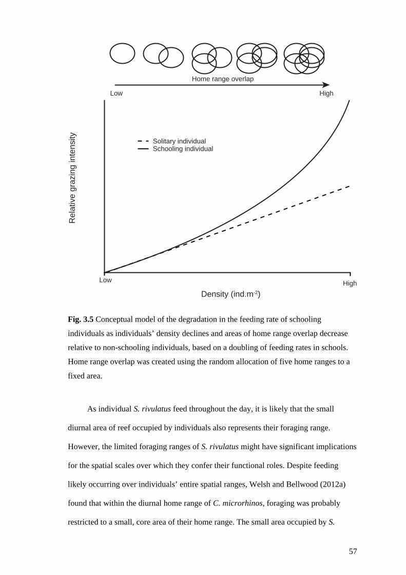
57
Fig. 3.5 Conceptual model of the degradation in the feeding rate of schooling
individuals as individuals’ density declines and areas of home range overlap decrease
relative to non-schooling individuals, based on a doubling of feeding rates in schools.
Home range overlap was created using the random allocation of five home ranges to a
fixed area.
As individual S. rivulatus feed throughout the day, it is likely that the small
diurnal area of reef occupied by individuals also represents their foraging range.
However, the limited foraging ranges of S. rivulatus might have significant implications
for the spatial scales over which they confer their functional roles. Despite feeding
likely occurring over individuals’ entire spatial ranges, Welsh and Bellwood (2012a)
found that within the diurnal home range of C. microrhinos, foraging was probably
restricted to a small, core area of their home range. The small area occupied by S.
Density (ind.m-2)
Relat
ive g
razin
g int
ensit
y
HighLow
Schooling individualSolitary individual
Home range overlap
HighLow
58
rivulatus suggests each fish’s contribution to herbivory, and thus ecosystem impact, on
the reef might likewise occur over a limited spatial range, and may be focused within an
even smaller core area of activity. In order to maintain localised functional processes at
sufficient rates to maintain reef resilience (Bellwood et al. 2004; Hughes et al 2005;
Graham et al. 2006; Ledlie et al. 2007), reefs require adequate home range overlap of
functionally important individuals (i.e. spatial redundancy). Traditionally, schools of
herbivores are assumed to provide spatial resilience, in that schools of fishes have been
assumed to move across large areas of reef and thus, act as mobile links. Mobile links
interconnect ecosystem processes over large spatial scales, and support resilience by
connecting degraded systems, where the vital processes for ecosystem recovery have
been compromised, to areas where the ecological processes are still operating (Nyström
and Folk 2001). However, our results suggest that the role of roving herbivore schools
as mobile links supporting functional processes may be weaker than previously
assumed.
Overall, our study demonstrates a clear, long-term pattern of site fidelity of not
only individuals, but also schools of a coral reef fish. While this study focused on
individuals from a single bay, recent evidence tends to suggest that these results may be
more broadly applicable. Nash et al (2012), found limited foraging range variability in
parrotfishes in response to variation in habitat condition. The nature of S. rivulatus
schooling is highly unstable, with little short-term school fidelity, but high long-term
fidelity to a shared area. Schooling behaviour appears to be the preferred social
condition, and has significant implications for the rate at which individuals contribute to
ecosystem functions to the reef. However, the limited spatial ranges described herein
suggest that these are only applied over a small area by an individual or even a school.
Schooling plays a significant role in facilitating elevated rates of key processes but
schooling behaviour is vulnerable to declines in local fish densities.
59
Chapter 4: The ontogeny of home ranges: evidence from
coral reef fishes Published in Proceedings of the Royal Society B 2013 76: 20132066
4.1 Introduction
Animal movement patterns are dynamic in space and time, and are a fundamental
component of a species’ ecology (Börger et al. 2008; Owen-Smith et al. 2010). With the
exception of migrations, most movements by animals are restricted to a home range.
However, this home range is rarely consistent over time and is likely to change as a
result of changing demands and abilities as the animal grows and matures (Johnson et
al. 2001; Jetz et al. 2004; Börger et al; 2008; Cagnacci et al. 2010). Throughout its life,
the size of any animal’s home range is driven by three key demands. Animals must
shape their home ranges to avoid predation, find adequate food and then, reproduce. As
animals grow, their body size changes their vulnerability to predators. In high-diversity
systems with a wide array of predators, smaller animals are more vulnerable and, as
such, must take steps to minimise predation risk. This can be accomplished by reducing
movement or avoiding risky locations, thus restricting an animal’s home range (Huey
1991; Broomhall et al. 2003; Imansyah et al. 2008). With growth, the range of potential
predators reduces, as does overall predation risk, which permits home range expansion
(Gagliano et al. 2007; Holmes et al. 2010). Similarly, as animals grow, the nutritional
demands of a larger body must be met, often demanding a greater area to procure
necessary food (White and Ralls 1993; Haskell et al. 2002; Carbone et al. 2011).
Finally, following maturation, an animal will need to find a mate and reproduce. Home
ranges, therefore, must be large enough to ensure adequate encounters with potential
mates (Trent and Rongstad 1974; Brown and Brooks 1993). While these drivers place
60
seemingly simple demands on an animal’s home range, the responses of animals are
complicated by concurrent ontogenetic shifts in physiological and social factors which
can also shape changes in home range size and patterns of utilisation. As such,
determining the relative importance of specific drivers in shaping changes in home
range sizes can be difficult.
Disentangling the various drivers and responses can be challenging. For example,
flight and associated high levels of parental care essentially remove the effects of
growth on the home ranges of fledged birds (Harrison and Roberts 2000). Similarly, in
mammals the effects of parental care and highly complex social systems often lead to
highly intertwined effects of home range drivers (Holekamp and Sherman 1989).
However, in lower vertebrates these drivers may be more clearly separated. For
example, varanid lizards (e.g. Komodo dragons, Varanus komodoensis) provide useful
models, as they undergo considerable growth following hatching and their home ranges
are less impacted by parental care than mammals or birds (Sumner 2006; Imansyeah et
al. 2008). Coral reef fish are another useful model to study the ontogeny of home
ranges. Following a brief period in the plankton, post-settlement fish grow by several
orders of magnitude on the reef, experiencing temporally separated events including
diet shifts, maturation and sex change. This temporal separation enables us to explore
the relative impact of predation, diet and reproduction on lower vertebrates using reef
fishes as a model.
In addition to understanding the factors affecting the ontogeny of home ranges, it
is crucial to understand the ecological consequences. Any shift in an animal’s home
range can profoundly impact its interactions with its environment (Owen-Smith et al.
2010; Bonaldo et al. 2012), as such, it is important to understand how these factors
change over the course of its life (Persson et al. 1998; Marshall et al. 2012). Coral reefs
in particular are highly reliant upon several functional groups of herbivorous reef fishes
61
to maintain their resistance and resilience to disturbances (Bellwood et al. 2004).
Parrotfishes (scarine Labridae), with their unique jaw morphology and numerical
abundance, dominate several of these functional groups (Bellwood et al. 2012). Recent
research, however, suggests that the ecosystem functions of parrotfishes depend on their
home ranging behaviour (Nash et al. 2012; Welsh and Bellwood 2012a). While it is
well documented that the role of herbivores changes with ontogeny (Chen 2002;
Bonaldo and Bellwood 2008; Lokrantz et al. 2008), it is not yet known a) how the home
range of an individual scales with body size, and b) which factors are most important in
determining changes in home range size through time.
This study examines the ontogeny of home ranges of three parrotfish species from
early post-settlement (approx. 10 mm, 0.01 g) to adulthood (over 300 mm and 1 kg).
This represents a change in mass of over five orders of magnitude, and incorporates a
dietary switch, from carnivory to detritivory, maturation and protogynous sex change.
During this time individuals are also subjected to distinct changes in predation risk,
social and reproductive demands (Bellwood 1988; Gagliano et al. 2007), and nutritional
needs (Bellwood 1988) which may also drive home range shifts. As such, these fishes
may provide novel insights into the relative importance of predation, nutrition and
reproduction, alongside other social factors, in shaping ontogenetic scaling of home
ranges in lower vertebrates.
4.2 Materials and Methods
Data collection
Field observations were conducted on Lizard Island, on the mid-shelf of the Great
Barrier Reef (14o41’5”S, 145o26’55”E). The primary study site was North Reef, an
obliquely exposed fringing reef extending from a distinctive crest (1 m below chart
62
datum) down to the reef base at 8-9 m. Home ranges were estimated for three species of
parrotfish (scarine Labridae; Cowman and Bellwood 2011), Scarus frenatus, S. niger
and Chlorurus sordidus. Home ranges were estimated from direct observations, using
three slightly differing methods, due to the wide range of size classes observed. Firstly,
for juvenile parrotfish (20-150 mm total length; TL) a scale map was used. The reef
front (approx. 80 m across) was mapped by recording prominent features, which were
used as reference points. The distances between reference points were measured, and by
triangulation, a two-dimensional scale map of the whole area created. Areas were
estimated based on a planar two-dimensional plot (where necessary the plot conformed
to any larger 3D surface complexity; landmark features would thus follow the benthos,
as a small fish would). The locations of fishes were subsequently recorded in relation to
the reference points. Where ranges were very small, additional reference points were
used to provide more detailed local maps.
Once a fish was located on the reef, it was identified to species, its size estimated
and any distinguishing features noted to allow individual identification (colour
markings and parasite scars were particularly useful). Each focal fish was followed for
a series of 30-min observation periods, marking its position every 15 s on a localised
scale map. These data points were then transferred onto overlays of the main scale map
and the area of the home range measured (as a convex polygon) using a digital graphic
pad. Individuals were followed for a minimum of four 30-min periods or until the
cumulative home range area (based on minimum convex polygons; MCP) reached an
asymptote (i.e. area occupied did not increase by more than 2%). This usually required
6-9 periods. No more than 2 observations were made per day, separated by at least three
hours. Ranges were estimated over a period of no more than 10 days, as they rapidly
expanded with fish growth. The cumulative area occupied over the entire observational
period was taken as the estimated home range. Due to low population densities of C.
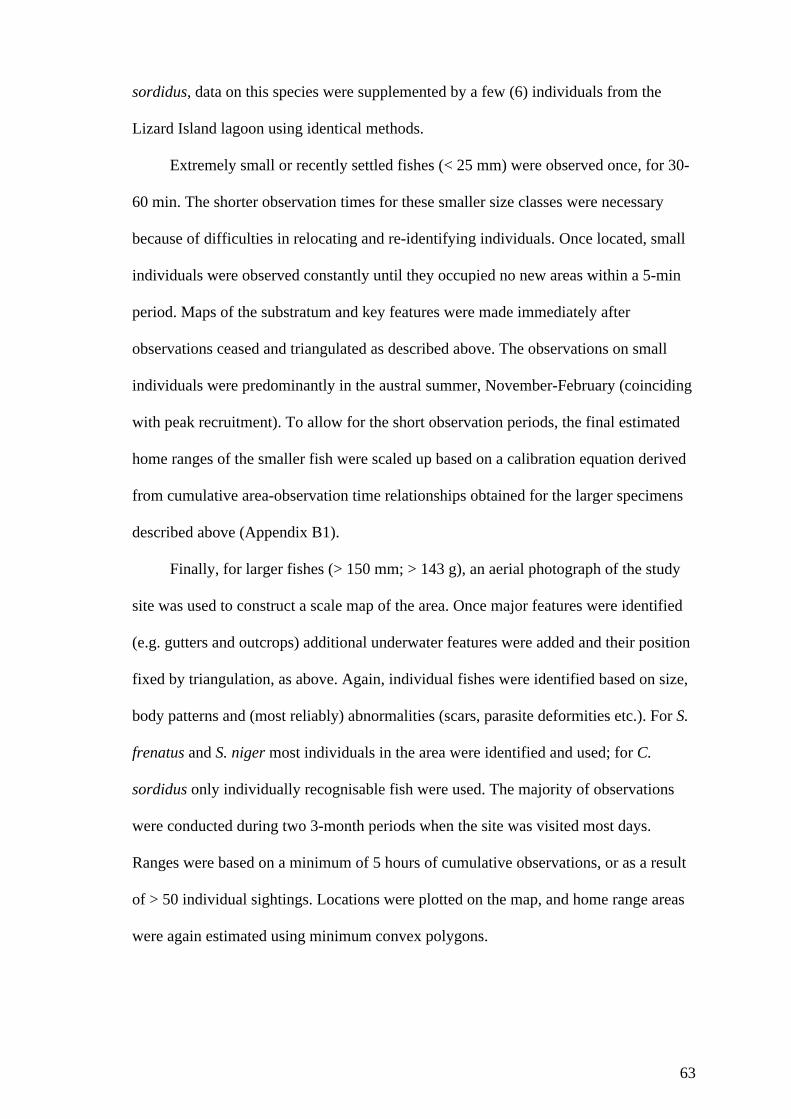
63
sordidus, data on this species were supplemented by a few (6) individuals from the
Lizard Island lagoon using identical methods.
Extremely small or recently settled fishes (< 25 mm) were observed once, for 30-
60 min. The shorter observation times for these smaller size classes were necessary
because of difficulties in relocating and re-identifying individuals. Once located, small
individuals were observed constantly until they occupied no new areas within a 5-min
period. Maps of the substratum and key features were made immediately after
observations ceased and triangulated as described above. The observations on small
individuals were predominantly in the austral summer, November-February (coinciding
with peak recruitment). To allow for the short observation periods, the final estimated
home ranges of the smaller fish were scaled up based on a calibration equation derived
from cumulative area-observation time relationships obtained for the larger specimens
described above (Appendix B1).
Finally, for larger fishes (> 150 mm; > 143 g), an aerial photograph of the study
site was used to construct a scale map of the area. Once major features were identified
(e.g. gutters and outcrops) additional underwater features were added and their position
fixed by triangulation, as above. Again, individual fishes were identified based on size,
body patterns and (most reliably) abnormalities (scars, parasite deformities etc.). For S.
frenatus and S. niger most individuals in the area were identified and used; for C.
sordidus only individually recognisable fish were used. The majority of observations
were conducted during two 3-month periods when the site was visited most days.
Ranges were based on a minimum of 5 hours of cumulative observations, or as a result
of > 50 individual sightings. Locations were plotted on the map, and home range areas
were again estimated using minimum convex polygons.
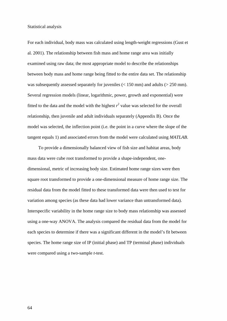
64
Statistical analysis
For each individual, body mass was calculated using length-weight regressions (Gust et
al. 2001). The relationship between fish mass and home range area was initially
examined using raw data; the most appropriate model to describe the relationships
between body mass and home range being fitted to the entire data set. The relationship
was subsequently assessed separately for juveniles (< 150 mm) and adults (> 250 mm).
Several regression models (linear, logarithmic, power, growth and exponential) were
fitted to the data and the model with the highest r2 value was selected for the overall
relationship, then juvenile and adult individuals separately (Appendix B). Once the
model was selected, the inflection point (i.e. the point in a curve where the slope of the
tangent equals 1) and associated errors from the model were calculated using MATLAB.
To provide a dimensionally balanced view of fish size and habitat areas, body
mass data were cube root transformed to provide a shape-independent, one-
dimensional, metric of increasing body size. Estimated home range sizes were then
square root transformed to provide a one-dimensional measure of home range size. The
residual data from the model fitted to these transformed data were then used to test for
variation among species (as these data had lower variance than untransformed data).
Interspecific variability in the home range size to body mass relationship was assessed
using a one-way ANOVA. The analysis compared the residual data from the model for
each species to determine if there was a significant different in the model’s fit between
species. The home range size of IP (initial phase) and TP (terminal phase) individuals
were compared using a two-sample t-test.

65
4.3 Results
The home ranges of 75 fish were estimated: 42 S. frenatus (15-356 mm TL), 14 S. niger
(11-304 mm TL) and 19 C. sordidus (10-240 mm TL). A logarithmic model was found
to provide the best fit for the relationship between body mass and home range size for
these three species (home range = 24.40 ln[body mass] + 55.58; Fig. 4.1), and was
considered to be the most biologically relevant. This model was significant, with body
mass explaining 76% of the variability in the home range data (r2 = 0.76; F1,73 = 236.44,
P < 0.001). The inflection point of the curve occurred when body mass equalled 24.4 ±
1.6 g. This corresponds to a length of 106.9 ± 4.4, 106.9 ± 4.4 and 107.0 ± 4.5 mm (TL
± error associated with the model) for S. frenatus, S. niger and C. sordidus respectively.
After this point, the rate of increase in home range per unit body mass was significantly
reduced. A power curve also provided a good statistical fit, but only for small
individuals; it explained little variation in larger specimens (Appendix B).
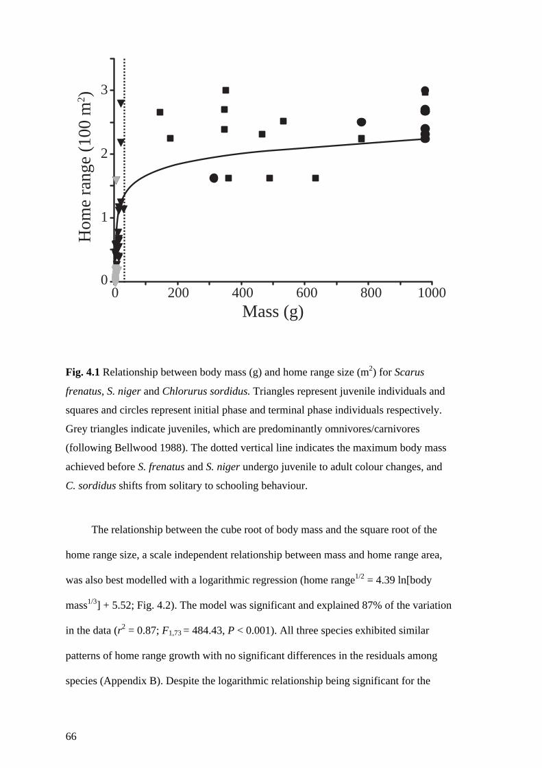
66
Fig. 4.1 Relationship between body mass (g) and home range size (m2) for Scarus
frenatus, S. niger and Chlorurus sordidus. Triangles represent juvenile individuals and
squares and circles represent initial phase and terminal phase individuals respectively.
Grey triangles indicate juveniles, which are predominantly omnivores/carnivores
(following Bellwood 1988). The dotted vertical line indicates the maximum body mass
achieved before S. frenatus and S. niger undergo juvenile to adult colour changes, and
C. sordidus shifts from solitary to schooling behaviour.
The relationship between the cube root of body mass and the square root of the
home range size, a scale independent relationship between mass and home range area,
was also best modelled with a logarithmic regression (home range1/2 = 4.39 ln[body
mass1/3] + 5.52; Fig. 4.2). The model was significant and explained 87% of the variation
in the data (r2 = 0.87; F1,73 = 484.43, P < 0.001). All three species exhibited similar
patterns of home range growth with no significant differences in the residuals among
species (Appendix B). Despite the logarithmic relationship being significant for the
Mass (g)0 200 400 600 800 1000
0
1
2
3H
ome
rang
e (1
00 m
2 )
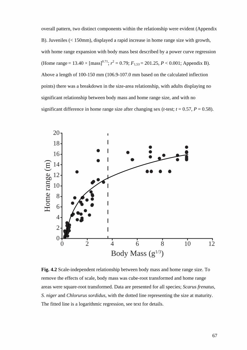
67
overall pattern, two distinct components within the relationship were evident (Appendix
B). Juveniles (< 150mm), displayed a rapid increase in home range size with growth,
with home range expansion with body mass best described by a power curve regression
(Home range = 13.40 × [mass]0.71; r2 = 0.79; F1,53 = 201.25, P < 0.001; Appendix B).
Above a length of 100-150 mm (106.9-107.0 mm based on the calculated inflection
points) there was a breakdown in the size-area relationship, with adults displaying no
significant relationship between body mass and home range size, and with no
significant difference in home range size after changing sex (t-test; t = 0.57, P = 0.58).
Fig. 4.2 Scale-independent relationship between body mass and home range size. To
remove the effects of scale, body mass was cube-root transformed and home range
areas were square-root transformed. Data are presented for all species; Scarus frenatus,
S. niger and Chlorurus sordidus, with the dotted line representing the size at maturity.
The fitted line is a logarithmic regression, see text for details.
Body Mass (g1/3)
Hom
e ra
nge
(m)
02468
101214161820
0 2 4 6 8 10 12

68
4.4 Discussion
We quantified the home range size of parrotfish species at every post-settlement stage
of their development, covering an increase in mass of over five orders of magnitude.
This increase in size leads to considerable shifts in predation risk, nutritional demands,
maturation and, in some individuals, a protogynous sex change (Choat and Robertson
1975; Booth and Beretta 2004; Depczynski and Bellwood 2005; Almany and Webster
2006; Gagliano et al. 2007), all of which can potentially drive changes in home range
size. Where ontogenetic effects on home ranges have been studied, the causes of the
changes have generally proved difficult to disentangle. Examples from birds and
mammals are hampered by relatively limited growth and a high degree of parental care
(Georgii and Schröder 1983; Jouventin and Weimerskirch 1990; Evans 2008).
Nevertheless, predation, nutritional needs and reproduction have been repeatedly
identified as key potential drivers (Jetz et al. 2004; Imansyah et al. 2008; Owen-Smith
et al. 2010; Avgar et al. 2013). In reef fishes, the clear separation of growth and
associated changes in trophic and sexual status may permit a better understanding of the
factors driving ontogeny of home ranges. As a result, we can begin to identify the roles
of potential drivers of home range size versus body mass relationships in one group of
lower vertebrates, the parrotfishes. In particular, three factors; predation, trophic and
reproductive demands, can be addressed separately.
Does predation restrict home ranges?
For small reef fishes, as with all small organisms, the risk of predation is extremely
high (Booth and Beretta 2004; Depczynski and Bellwood 2005; Almany and Webster
2006). In such a hazardous environment as a coral reef, fishes face a trade-off between
foraging and remaining in, or near, shelter (Booth and Beretta 2004; Leahy et al. 2011).
69
Predation pressure is therefore likely to limit movement in small fishes (Depczynski
and Bellwood 2004). As they grow, however, larger body size enables home range
expansion, probably as a result of increasing handling costs for predators seen in both
reef fishes (Holmes and McCormick 2010) and forest birds, such as the junco (Junco
phaenotus; Sullivan 1989). Therefore, if predation was the primary mechanism driving
the mass-area relationship in parrotfishes, we would expect initially slow expansion of
home ranges in juveniles, followed by a rapid increase in the area occupied as fish grew
and predation risk declined. This is not the case for juvenile parrotfish, as they rapidly
expand their home range from the smallest size observed. The breakdown in the
relationship observed in larger fishes (> 100-150 mm) may result from a size threshold
above which a new suite of predators becomes important. However, this seems unlikely
as reef predators are capable of handling a wide size range of prey, with the vast
majority targeting small fishes (Almany and Webster 2006; Holmes and McCormick
2010). Overall, home ranges do not expand in a manner consistent with decreasing
predation. This suggests that other factors such as food availability may be more
important.
Trophic constraints on home ranges
Rapid expansions of home range with body size, comparable to those seen in juvenile
scarids, are occasionally observed in species seeking food resources when food is
limiting. This has been seen in many reptile species including Komodo dragons
(Imansyah et al. 2008), and some mammalian species, including ground squirrels
(Holekamp and Sherman 1989; Haskell et al. 2002; Börger et al. 2008), all of which
forage for widely dispersed, cryptic food resources. Small parrotfishes inhabit the
epilithic algal matrix (EAM) following settlement (Bellwood and Choat 1989), preying

70
on small cryptobenthic crustaceans and other invertebrates (Bellwood 1988). While
these invertebrates are highly abundant on coral reefs (Kramer et al. 2012), the rate at
which small parrotfish expand their home ranges suggests that not all invertebrates are
available to the fish and that larger ranges are needed to access adequate food resources.
The complex 3-dimensional structure of the EAM might provide shelter for the prey.
This, in conjunction with the limited gapes and jaw strength of juvenile parrotfishes
(Bonaldo and Bellwood 2008) suggests that they are only able to detect and acquire
prey close to the surface of the EAM. Thus, a larger home range would be required to
increase prey encounter rates. This type of demand has previously been documented in
cheetahs (Broomhall et al. 2003), and is especially prevalent in taxa with insectivorous
life stages, such as tropical lizards (Rocha 1999; Imansyah et al. 2008). Despite insects
being highly abundant on land, their availability is patchy and consequently, terrestrial
insectivores require large home ranges to encompass sufficient resources. Parrotfish
follow this pattern throughout their invertivorous stage, suggesting that the distribution
of available invertebrate prey might be comparably sparse or patchy.
Larger juveniles continue to exhibit rapid home range expansions with body
mass, despite a marked dietary shift from crustaceans to detritus and algae (based on
specimens collected from this study location; Bellwood 1988). Juvenile scarids possess
small beaks and as such can only make relatively shallow bites (Bonaldo and Bellwood
2008). With their limited bite size, juvenile parrotfish may therefore have to make a
disproportionately large number of bites over a large area to ingest sufficient nutrients
or to seek out patches of high quality EAM, with low sediment loads and a high detrital
component (Wilson et al. 2003). Again, large home ranges would increase the chances
of encountering sufficient high-quality food.
Overall, it would appear that the relationship between somatic size and the home
ranges of juvenile parrotfish is influenced primarily by the need to acquire high quality
71
resources rather than directly avoiding predation risk. However, predation pressure may
be indirectly involved. By accessing a large quantity of resources of the highest
nutritional quality, juveniles are able to grow rapidly, minimising the time they must
spend in life stages that are subject to the highest rates of predation.
Following maturation, home ranges cease to expand at the same rate. The reason
for this may, in part, be due to parrotfish functional morphology. The strength and size
of adult parrotfish beaks is significantly greater than their juvenile counterparts
(Bellwood and Choat 1990). This allows them to bite deeper into the EAM, removing
greater volumes of algae, invertebrates and particulate organic matter (Bellwood 1988;
Choat et al. 2004; Kramer et al. 2013). By adding a new dimension (depth) to their
feeding, it appears that adult parrotfish can access more resources per area than
juveniles which can only scrape the surface (Bonaldo and Bellwood 2008). Similar
changes in function are observed in terrestrial and marine retiles, with potential impacts
on their home ranges (Herrel et al. 2006; Imansyah et al. 2008; Marshall et al. 2012).
While changing functional capabilities may provide an explanation of why home range
expansion can cease, it does not explain the relatively rapid transition. This appears to
be driven by social interactions.
Reproductive constraints on home ranges
Between 100 and 150 mm, the relationship between somatic size and home range
changes and parrotfishes exhibit a marked ontogenetic shift in their home ranging
behaviour. Adult fishes had home ranges between 160 and 300 m2, which are broadly
comparable to other Pacific and Atlantic parrotfishes (van Rooij et al. 1996; Mumby
and Wabnitz 2002). If home range expansion continued to follow the pattern seen in the
juveniles, an individual would occupy approximately 16,000 m2 by the time it reached
72
300 mm (TL). This is over 50 times larger than any home range found in adults. Why
home ranges cease to expand with body size is particularly interesting and raises several
questions: how are adults able to acquire sufficient resources to meet metabolic
demands, especially given that juveniles respond to their environment as if they are
resource limited, and what mechanism drives the marked change in the relationship?
The social status of parrotfishes directly influences their ecology (van Rooij et al.
1996; Muñoz and Motta 2000; Bonaldo and Krajewski 2008), and may be responsible
for limiting home range expansions in adult fishes (Afonso et al. 2008; Welsh and
Bellwood 2012a). The breakdown in the area-mass relationship corresponds closely
with reported colour changes in two of the three focal species. These colour changes are
associated with the transition from juvenile to initial phase adults, and occur at
approximately 120 mm for both S. frenatus and S. niger (Sullivan 1989). Following
colour changes, the new initial phase adults of these species join small social groups, or
harems, with a single aggressive male defending a fixed territory. This social transition
corresponds closely with the changing area-mass relationship observed in our study,
where the home ranges of relatively small individuals rapidly increase until they match
the size of the harem leader’s territory. Thereafter, home ranges no longer increase with
an individual’s somatic size. This pattern of territorial range delineation has been
recorded in a number of other social taxa such as cheetahs (Acinonyx jubatus;
Broomhall et al. 2003), red deer (Cervus elaphus; Georgii and Schöder 1983) and
coyotes (Canis latrans; Messier and Barrette 1982), in which young individuals occupy
the territory of their parents or social group (Marler et al. 1995; Mumby and Wabnitz
2002; Hinsch 2013). This social control of home range expansion after maturity might
be the reason we see no evidence of an effect of the change in sex (and colour)
associated with a transition from initial to terminal phase in adult parrotfishes.

73
C. sordidus does not exhibit drastic colour changes as they transition from the
juvenile to initial phase, and do not form aggressively defended harems. However, at
around 90 mm long, juveniles of this species shift from being solitary occupants of
sheltered back-reefs or deeper areas, to schooling, mature adults, most frequently
occupying shallow, exposed fore-reefs (Sullivan 1989). In parallel with this behavioural
shift, the area-mass relationship again changes abruptly, as seen in the haremic species.
While schooling species have significantly fewer aggressive interactions, they too
remain site attached as adults, apparently occupying areas of familiarity to facilitate
escape from predators or aggression from other species (Choat and Bellwood 1985;
Welsh and Bellwood 2012b).
Many studies have highlighted the predictability of the mean home range size of a
species, given its average body size; a standard interspecific scaling relationship (Rocha
1999; Haskell et al. 2002; West and West 2012). Within species, however, marked
changes in the rate of home range expansion are often associated with ontogenetic
changes in diet. Reptiles are among the best examples of this phenomenon, with some
species exhibiting wholesale shifts in diet, habitat and home ranging behaviour as they
increase their body mass (Herrel et al. 2006; Imansyah et al. 2008). In the parrotfishes,
the cessation of home range expansion, despite continued somatic growth, is markedly
different. In parrotfishes, the effect of changing diet or predation risk seems to have
little influence on spatial utilization patterns. Instead, for adult parrotfishes, complex
social systems appear to drive their home range-size relationships; a pattern with strong
parallels to those relationships seen in social birds and mammals. In birds, mammals
and other taxa living in social groups, the size of a social group’s territory is often
described as a ‘minimum economically defensible area’ where all members of a social
group have access to the group’s entire territory (Johnson et al. 2001; Clutton-Brock et
74
al. 2008). In these examples, as in parrotfishes, body size does not play a significant
role in determining the home range size of an individual within the group.
The present study highlights the need to assess the spatial behaviour of organisms
at all stages in their growth and development in order to understand the nature of home
ranging behaviour. With growth, juvenile parrotfishes displayed rapid increases in
home range size which appears to be driven by increased nutritional demands. A
distinct change in the rate of home range expansion mirrors changes in colour patterns
and appears to be shaped primarily by social factors associated with sexual maturity
(Sullivan 1989), while changes in body size, diet and sex appear to have a limited
impact on the overarching area-size relationship. Overall, juvenile parrotfishes operate
like forest dwelling lizards, while adults operate like social mammals. Our observations
suggest that for fishes, inter- and intra-specific size-area relationships may be shaped by
markedly different drivers.
75
Chapter 5: Herbivorous fishes, ecosystem function and
mobile links on coral reefs Published in Coral Reefs 2014 33: 303-311
5.1 Introduction
Many studies have emphasised the need to increase resilience to help limit or prevent
ecosystem decline (Vitousek et al. 1997; Scheffer et al. 2001). The resilience of an
ecosystem refers to the capacity of the system to respond to, and recover, after a
disturbance event (Folke et al. 2004; Hughes et al. 2003, 2007). To be resilient, a
system must have the ecological capacity to maintain critical ecosystem processes
(Hughes et al. 2003; Carpenter et al. 2006). One key component of resilience is
connectivity via mobile links (Lundberg and Moberg 2003; Rico et al. 2012). Mobile
links are described as those taxa which have the capacity to move between systems,
particularly where they supplement functional processes by moving from a relatively
intact system to one degraded by exploitation or natural disturbances (Lundberg and
Moberg 2003). Mobile links may be passive (e.g. marine invertebrate larvae) or active
(e.g. bats, birds and large terrestrial herbivores), depending on their capacity for
movement (Lundberg and Moberg 2003; Couvreur et al. 2004; Kremen 2005;
Sekercioglu 2006).
In the marine environment, the passive mobile links of invertebrates and the more
active larval fishes have been widely studied, and their ability to interconnect reefs is
well established (e.g. Jones et al. 1999; Patterson and Swearer 2007; Almany et al.
2009). These larval connections are usually over large spatial and temporal scales
(regional to biogeographic scales, over weeks to years) (Patterson and Swearer 2007;
Shanks 2009). In contrast, the reef-scale, short-term movement or connectivity of adults
76
has received less attention, and the extent and nature of active mobile links in the
marine environment is poorly understood. This is especially troubling on coral reefs
given the potential importance of ecological interactions conferred by one of the key
active mobile links, roving herbivorous reef fishes (e.g. Nyström and Folke 2001;
Ceccarelli et al. 2011).
Reef fishes have a number of functional roles, which support the resilience of
coral reef ecosystems (Bellwood et al. 2004; Folke et al. 2004). One key process is
herbivory, where the feeding activities of herbivorous fish mediate coral-algae
interactions and help maintain a coral dominated state (McCook 1997; Bellwood et al.
2004; Burkepile and Hay 2010). Within the herbivore guild, separate functional groups
have been identified, each important in maintaining different components of reef
resilience. Scrapers (e.g. Scarus spp.), excavators (e.g. Chlorurus spp.) and croppers
(e.g. Acanthurus spp.) are responsible for grazing the reef’s epilithic algal matrix and
keeping algal growth in check (Fox and Bellwood 2007). Browsers (e.g. Kyphosus spp.)
are unusual in that they feed directly on adult leathery macroalgae, and play an
important role in the removal of macroalgae (Bellwood et al. 2004; Burkepile and Hay
2008; Hoey and Bellwood 2009; Rasher et al. 2013). Given its importance in
regenerating degraded ecosystems, a great deal of research has recently been focused on
quantifying the browsing functional role (e.g. Burkepile and Hay 2010; Michael et al.
2013), especially on the GBR (McCook 1997; Hughes et al. 2007; Hoey and Bellwood
2009). This research has found that the process is overwhelmingly dominated by a
limited number of species (predominantly Naso unicornis and Kyphosus vaigiensis),
and that it is highly variable both spatially and temporally (Cvitanovic and Bellwood
2009; Bennett and Bellwood 2011; Lefèvre and Bellwood 2011). Understanding the
nature of this variability is key to understanding how browsing herbivores interact with
their environment, support its resilience and offer a capacity to regenerate or recover

77
from degradation. However, the factors that underpin this variability remain to be
determined and are likely to be strongly influenced by the spatial scales over which
browsing herbivores feed.
In the terrestrial environment, large bodied herbivorous mammals will travel
several hundred kilometres in search of food. They act as mobile links, delivering both
their grazing activities and ingested plant seeds to distant, spatially separated locations,
and thus interconnect metapopulations (Couvreur et al. 2004; Owen-Smith et al. 2010).
On coral reefs, there is no evidence of similar widespread feeding behaviour and thus,
little evidence that fishes act as mobile links in this manner (but see Vermeij et al.
2013). Indeed, most reef fishes, including roving herbivores, appear to have extremely
limited movements (Eristhee and Oxenford 2001; Meyer and Holland 2005; Fox and
Bellwood 2011; Welsh and Bellwood 2012a, b). The basic question in understanding
functionally important mobile links on coral reefs is: at what point is an individual’s
home range large enough for them to act as a significant vector for functional
connectivity (i.e. a mobile link)?
Evidence of a relationship between body length and a fish’s home range length
has been used to identify the size range of fishes which are expected to be protected by
a MPA of a given size (Kramer and Chapman 1999). This relationship highlights the
limited movement of many smaller species, a finding that has been strongly supported
by recent studies, which have employed acoustic telemetry to assess the movement
patterns of individual herbivorous fish species. These studies have invariably found that
the movements of reef species are constrained to relatively small areas of reef,
regardless of the fish’s social characteristics (e.g. haremic or schooling) and thus, these
species may contribute little to functional connectivity (Afonso et al. 2008; Hardman et
al. 2010; Welsh and Bellwood 2012a, b). Indeed, the traditional distinction between
small solitary and large roving herbivores appears to be largely a reflection of size and
78
even the largest ‘roving’ herbivores do not move very far, even when foraging in
schools (Welsh and Bellwood 2012a). Therefore, most fishes on coral reefs may not be
mobile links at all, a sobering notion given that large-scale movements by herbivores
have been described as being among the most important mobile links on coral reefs
(Nyström and Folke 2001).
Our goal, therefore, was to: a) determine if all major nominal reef herbivore
groups show comparably small range sizes and b) to contextualize the movements of a
functionally important herbivorous species, K. vaigiensis, with those reported for other
coral reef species in the primary literature. To evaluate the first objective, we assess
home range data on a largely overlooked family of coral reef herbivores, the
Kyphosidae. We then compare these home range data to published home range sizes of
representative species from every major herbivore family and to a broad range of non-
herbivore species. With this information, we provide an overview of herbivorous
mobile links on coral reefs in order to better understand potential connectivity of
functional processes on an inter- and intra-reef scale, and discuss the implications of
how this may influence the predicted local-scale ecosystem benefits of MPAs.
5.2 Materials and Methods
Home range of Kyphosus vaigiensis
This study took place between September 2011 and January 2012 on the fringing reefs
surrounding Orpheus Island (18°350’S, 146°200’E), an inshore island on the GBR. The
majority of the spatial sampling effort occurred within Pioneer Bay, on the leeward side
of Orpheus Island, with an extensive reef flat and a moderately complex reef structure
(detailed descriptions of Pioneer Bay are given in Welsh et al. 2012).

79
Acoustic monitoring
The movements of K. vaigiensis around Orpheus Island were quantified using acoustic
monitoring. This involved the construction of an array of 46 acoustic receivers (VR2W;
Vemco, Halifax, Canada), deployed around Orpheus Island (Fig. 5.1a). The majority of
the receivers (25 × VR2Ws) were placed within Pioneer Bay to provide a high-
resolution indication of tagged individual’s activities within the bay (Fig. 5.1b). The
remaining receivers (15 × VR2Ws) were moored at key monitoring positions around
the island, i.e. the points and centres of nearly every bay (Fig. 5.1a). Six additional
receivers on adjacent islands (three on Pelorus and three on Phantom) had no
detections. The effective detection range (where 50% of acoustic signals are detected)
of the receivers was assessed and found to be approximately 55 m throughout the
duration of the study (Welsh et al. 2012).
Prior to tagging, the population size of K. vaigiensis was estimated. To ensure an
accurate estimation of the proportion of the population of K. vaigiensis being sampled,
five 1.4 km x 15 m snorkel transects (spanning the entire length of Pioneer Bay) were
conducted along the reef crest. A 15 m width was selected to ensure that widths could
be maintained regardless of visibility over the census days. Each census was undertaken
on non-consecutive days.
Individual K. vaigiensis were captured by divers on SCUBA from four separate
sites over a 1.4 km stretch of reef within Pioneer Bay using barrier nets in September
2011 (Fig. 5.1b). Four capture sites were used to maximize the chances of sampling fish
from separate schools. Once captured, fish were transported to the Orpheus Island
Research Station where they were held in 3300 L flow-through tanks prior to surgical
tagging. To tag the fish, individuals were first anaesthetised in a tricane
methanesulfonate (MS-222) seawater solution (0.13 gL-1). Once the fish was sedated,

80
the fork length (FL) was recorded and a small incision was made in the body wall. An
ultrasonic transmitter (tag; V9-1L, random delay interval 190-290 s, power output 146
dB re 1 µPa at 1m, Vemco) was then inserted into the peritoneal cavity of the
individual, and the incision was sutured closed and treated with antiseptic. Following
surgery, individuals were held in captivity for 12-24 h to recover before being released
back at their site of capture.
Fig. 5.1 Orpheus Island receiver (VR2W, Vemco) deployment sites. Black circles mark
the location of each receiver. Filled in circles represent receivers with > 5% of at least
one individual Kyphosus vaigiensis’ detections; open circles had no significant
detections. a) Map of Orpheus Island with large-scale receiver placements. b) Array in
Pioneer Bay showing depth contours and numbered stars representing capture and
release sites of individuals (capture site 1: K40, K41, K42, K43, K44; capture site 2:
K31, K32, K35; capture site 3: K36, K37, K38, K39; capture site 4: K33, K34). Dotted
lines represent reef area.
800 m
Orpheus Island
400m
0.5m
0m
5m
1.1m0.6m
1m
0.8m
0.8m
1.3m
0.8m
0.6m
0.6m
1.1m
N
4
32
1
3
b Pioneer Bay
a
81
Before the data were analysed, each individual's detection plots were inspected
using the VUE software package (Vemco) to check for signs of mortality. Mortality
was identified by an obvious change in an individual’s movement patterns to long
periods of inactivity. If mortality was suspected, all subsequent detections were
excluded from the analyses (one individual was excluded on this basis; Appendix C).
For analysis, the first 24 hours of data from each individual following release was
excluded to remove any unusual behaviour, which may arise from tagging. Each
individual’s detection data were then separated into diurnal and nocturnal sampling
periods. Diurnal periods were set from 05:30 to 19:30 h to incorporate crepuscular
movements and nocturnal periods were defined as 19:31 to 05:29 h. The frequency and
variability of large-scale movements were analysed using the adehabitat LT package for
R (Calenge 2006). The home range length of each individual was calculated for diurnal
and nocturnal periods using two metrics: the minimum linear dispersal (MLD) and the
median distance travelled (MDT). Both metrics were calculated using adehabitatLT.
The MLD is defined as the shortest possible distance between the two most distant
receivers where an individual has been detected (Murchie et al. 2010). For the purposes
of this study, this metric will be used to represent the minimum home range length. The
MDT provides a metric of the median dispersal of an individual from its principal area
of residence. Individual’s MDT values were quantified by first determining the receiver
on which an individual is most frequently detected, and then calculating the median
distance between that receiver and all other receivers where the fish was detected
(Murchie et al. 2010). The proportion of detections at an individual’s principal
detection location was also calculated for each individual in diurnal and nocturnal
periods to compare how stationary or site-attached individuals are at night versus the
day. To meet the assumptions of the parametric t-test, MLD data were log-transformed
and a logit-transformation was applied to the proportion data (Warton and Hui 2011).
82
To further explore individual movement patterns, we calculate the average number of
detections per day for each individual at each of the VR2W acoustic receivers. These
detection frequencies were calculated for diurnal and nocturnal periods. The
distribution of detections (expressed as a coefficient of variation [CV = standard
deviation / mean] for each individual) provides a representation of the spread of the
movements of each individual K. vaigiensis throughout their home range. High CV
values indicate a heterogeneous distribution of an individual’s detections throughout the
acoustic array, while low CV values suggest that the distribution is more homogeneous.
All the above metrics were calculated using the data set for the entire study period.
However, for each individual, the average MLD was also calculated over 5 separate
randomly selected days to quantify the average size of an individual’s daily movements.
A t-test for matched pairs was used to compare the diurnal and nocturnal
sampling periods for the overall MLD, the daily MLD, and the proportion of detections
at individual principal detection locations. The CV values for each individual were also
compared between diurnal and nocturnal samples using a t-test for matched pairs.
Data for general home range relationship
To evaluate the potential of herbivorous reef fishes to act as mobile links, a dataset of
published coral reef fish home range length data was assembled by searching the ISI
Web of Science and Google Scholar for primary research articles using the following
keywords: fish, coral reef, home range, movement, spatial. Studies were limited to
those conducted on adult coral reef taxa that provided an estimation of the linear
movements of focal taxa. Studies on adult reproductive migrations were excluded. The
selection criteria avoided confounding factors associated with ontogenetic home range
expansion and reproductive behaviour. Furthermore, data were excluded if individuals
83
did not survive for > 24 h following release after tagging and/or if based on homing
studies, as these cases would most likely represent unusual behaviour. From each study,
the maximum distanced moved by any individual of each species was recorded along
with the individual’s corresponding body size (measured as fork length) following
Freiwald (2012). The functional group was also noted and classified as either carnivore
or herbivore. If several studies were available for the same species, the study that
reported the largest movement, meeting the aforementioned criteria, was used.
Body size data exhibited a non-normal (positively skewed) distribution. Data
were therefore square root transformed to normalize the data. The relationship between
body size and home range length was analysed using GLMs in (lme4 package in R;
Bates & Maechler 2009; R Development Core Team 2011). Initially, an overall model
was constructed irrespective of functional group. Separate models were then
constructed for each functional group. To test for deviations from each model, an
analysis of each species’ Cook’s Distance was used (Quinn and Keough 2002).
5.3 Results
Home range of Kyphosus vaigiensis
In total, 14 individual K. vaigiensis (average length 29.4 ± 0.7 cm SE; range 23.4-32.6
cm) were tagged. This represented approximately 10% of the total within-bay
population size, which was estimated to be 148.4 ± 8.8 individuals. Over the 5-month
study, individual K. vaigiensis exhibited consistently large home ranges regardless of
capture site. Individuals travelled an average minimum linear distance (MLD) of
2,521.4 ± 713.7 m during the day and 2,625.9 ± 880.1 m at night (and ranging from 784
to 13,352 m; Fig. 5.1; Table 5.1; Appendix C). These values were extensive and, on
average covered over 10% of the available coastline of Orpheus Island for both diurnal
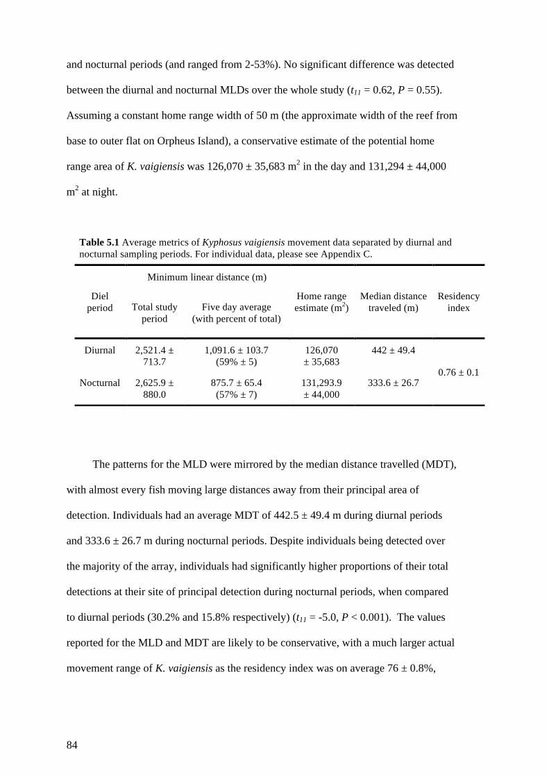
84
and nocturnal periods (and ranged from 2-53%). No significant difference was detected
between the diurnal and nocturnal MLDs over the whole study (t11 = 0.62, P = 0.55).
Assuming a constant home range width of 50 m (the approximate width of the reef from
base to outer flat on Orpheus Island), a conservative estimate of the potential home
range area of K. vaigiensis was 126,070 ± 35,683 m2 in the day and 131,294 ± 44,000
m2 at night.
The patterns for the MLD were mirrored by the median distance travelled (MDT),
with almost every fish moving large distances away from their principal area of
detection. Individuals had an average MDT of 442.5 ± 49.4 m during diurnal periods
and 333.6 ± 26.7 m during nocturnal periods. Despite individuals being detected over
the majority of the array, individuals had significantly higher proportions of their total
detections at their site of principal detection during nocturnal periods, when compared
to diurnal periods (30.2% and 15.8% respectively) (t11 = -5.0, P < 0.001). The values
reported for the MLD and MDT are likely to be conservative, with a much larger actual
movement range of K. vaigiensis as the residency index was on average 76 ± 0.8%,
Table 5.1 Average metrics of Kyphosus vaigiensis movement data separated by diurnal and nocturnal sampling periods. For individual data, please see Appendix C.
Diel period
Minimum linear distance (m)
Home range estimate (m2)
Median distance traveled (m)
Residency index Total study
period Five day average
(with percent of total)
Diurnal 2,521.4 ± 713.7
1,091.6 ± 103.7 (59% ± 5)
126,070 ± 35,683
442 ± 49.4
0.76 ± 0.1 Nocturnal 2,625.9 ±
880.0 875.7 ± 65.4
(57% ± 7) 131,293.9 ± 44,000
333.6 ± 26.7
85
indicating that individuals were beyond the detection regions of the array 24% of the
time on the days analysed (Table 5.1).
The distributions of an individual’s average daily detections were highly variable,
with detections over 24 h spread across the majority of the acoustic array. However,
when evaluated in diurnal versus nocturnal subsections, it was clear that species were
generally more mobile in diurnal sampling periods (Appendix C). Diurnal samples were
characterized by records at a number of receivers. Nocturnal samples usually had a
major location and relatively few records at other receivers. This is supported by CV
values, which were significantly lower over diurnal samples (mean = 1.76) compared to
nocturnal samples (mean = 2.50; t13 = -3.22, P < 0.01).
Daily movement patterns
When only a single 24 h period was considered (with 5 random days used for
replication), individual’s MLD values were quite large, with an average of 1,091.6 ±
103.7 m and 875.7 ± 65.4 m, during diurnal and nocturnal periods respectively.
Individual’s 24 h subsample movements values were, on average, 59% of an
individual’s total diurnal MLD and 57% of an individual’s total nocturnal MLD (Table
5.1; Appendix C). The average 24 h MLD values of each individual were significantly
different when comparing diurnal and nocturnal movements (t11 = 3.02, P = 0.01), with
most individual’s diurnal movements being larger (Appendix C).
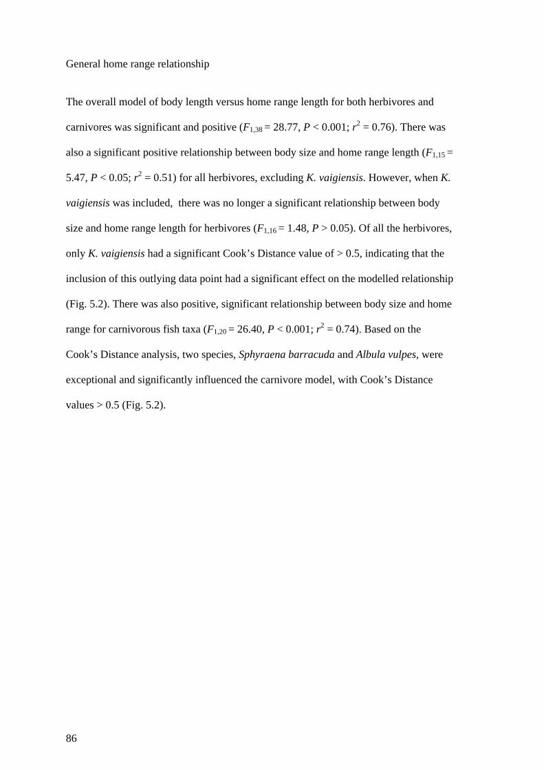
86
General home range relationship
The overall model of body length versus home range length for both herbivores and
carnivores was significant and positive (F1,38 = 28.77, P < 0.001; r2 = 0.76). There was
also a significant positive relationship between body size and home range length (F1,15 =
5.47, P < 0.05; r2 = 0.51) for all herbivores, excluding K. vaigiensis. However, when K.
vaigiensis was included, there was no longer a significant relationship between body
size and home range length for herbivores (F1,16 = 1.48, P > 0.05). Of all the herbivores,
only K. vaigiensis had a significant Cook’s Distance value of > 0.5, indicating that the
inclusion of this outlying data point had a significant effect on the modelled relationship
(Fig. 5.2). There was also positive, significant relationship between body size and home
range for carnivorous fish taxa (F1,20 = 26.40, P < 0.001; r2 = 0.74). Based on the
Cook’s Distance analysis, two species, Sphyraena barracuda and Albula vulpes, were
exceptional and significantly influenced the carnivore model, with Cook’s Distance
values > 0.5 (Fig. 5.2).
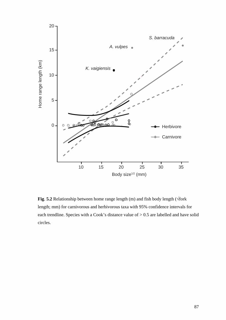
87
Fig. 5.2 Relationship between home range length (m) and fish body length (√fork
length; mm) for carnivorous and herbivorous taxa with 95% confidence intervals for
each trendline. Species with a Cook’s distance value of > 0.5 are labelled and have solid
circles.
Hom
e ra
nge
leng
th (k
m)
10
5
15
20
0
10 15 20 25 30 35Body size1/2 (mm)
K. vaigiensis
A. vulpes
S. barracuda
Carnivore
Herbivore
88
5.4 Discussion
Despite our rapidly increasing knowledge of the spatial ecology of marine taxa, no
herbivorous species on coral reefs have been quantitatively identified as mobile links as
adults. Most reef fishes remain close to the structure provided by the reef and have been
shown to be less willing than their terrestrial counterparts to cross gaps in shelter of
more than 20 m (Meyer et al. 2010; Turgeon et al. 2010). Among herbivores, K.
vaigiensis appears to be an exception to this rule, being sufficiently vagile to travel
large distances, not only across the reef within a single bay, but also between fringing
reefs up to 11 km apart. It is, to our knowledge, the only documented coral reef
herbivore to-date capable of providing short-term reef-scale connectivity of functional
processes.
The association between body size and home range length highlights the site-
attached nature of reef fishes, especially the herbivores, the presumed mobile links.
Even one of the largest herbivores, Naso unicornis, is predicted by the herbivore model
to occupy a range of just 1,024 (± 381.84) m (linear home range). A finding strongly
supported by several studies of the species (estimating its range to be between 240 and
940 m long) and highlighting its site-attached behaviour (e.g. Meyer and Holland 2005;
Hardman et al. 2010). Most herbivores, therefore, appear to contribute little as mobile
links. However, K. vaigiensis, a functionally important herbivorous reef fish
(Cvitanovic and Bellwood 2009; Hoey and Bellwood 2011), appears to depart
significantly from the expected body size - home range length relationship. It is a
significant outlier for a herbivorous species, with a range over three times larger than
expected based on its size. The distances moved by this species are more similar to
those of the pelagic carnivorous species, Sphyraena barracuda (O’Toole et al. 2011)
and Albula vulpes (Murchie et al. 2013), which were likewise the only other taxa that
deviated significantly from the predicted relationship for non-herbivore fishes. It is by
89
virtue of these unusual, large-scale (i.e. > 2 km) daily movements that K. vaigiensis
may be important for the functional connectivity within reefs, serving as an active
mobile link and thereby able to contribute significantly to reef resilience across a range
of spatial scales.
The importance of the unique, large-scale movement of K. vaigiensis is most
apparent when placed in context of its functional role. The role of browsing herbivores
is one in which functional redundancy (i.e. niche overlap of several taxa performing the
same functional role) is extremely limited (Hoey and Bellwood 2009). On the GBR, the
removal of adult macroalgae is restricted to between two and six species (Bellwood et
al. 2006; Mantyka and Bellwood 2007), although often only one two species are
predominant in a single area (Cvitanovic and Bellwood 2009; Hoey and Bellwood
2010). Among these few species, K. vaigiensis stands out consistently as a significant
predator of macroalgae (Cvitanovic and Bellwood 2009; Lefèvre and Bellwood 2011).
Indeed on several occasions, this species and its congenerics have been noted to play a
vital role in coral reef resilience through intense predation of macroalgae (Downie et al.
2013; Michael et al. 2013). The exceptional mobility of a single species within this
vitally important ecological role for reef health suggests that short-term mobile links in
adult herbivores may be particularly rare on coral reefs.
Home range size in reef fishes
Herbivorous fishes have previously been recognized as important mobile links for
functional processes (Nyström and Folke 2001; Lundberg and Moberg 2003). However,
this may not be the case for most species. Only K. vaigiensis exhibited attributes that
would enable it to act as a mobile link, providing large-scale ecosystem connectivity by
interconnecting ecological processes on reefs up to 11 km apart. Observations of the
90
behaviour of K. vaigiensis at this site found that it invariably travels in large schools
(>20 individuals). Therefore the large home ranges exhibited by the tagged individuals
are likely to be representative of a significant proportion of the population.
On average, K. vaigiensis occupies a stretch of reef 2,521 m long. This is
approximately 2 to 100 times larger than other roving herbivorous species. In
comparison, the home ranges of several similarly-sized territorial or haremic
herbivorous species, such as Chlorurus microrhinos from the GBR (Welsh and
Bellwood 2012a), Sparisoma cretense in the mid-Atlantic (Afonso et al. 2008) and S.
viride from the Caribbean (van Rooij et al. 1996), have been found to be relatively
small, with home range lengths of just 266, 460, and 25 m respectively. These restricted
ranges likely occur as a result of the trade-off between the energetic expenditure of
territorial defence and the benefits of exclusive access to a territory’s resources. These
benefits become unfavourable when too large an area must be defended (Bonaldo et al.
2006; Laguë et al. 2012). We would therefore expect smaller, limited home ranges in
territorial or haremic species. However, even schooling, non-territorial species also
seem to have quite limited home range sizes. The schooling parrotfish Scarus rivulatus
in the GBR (Welsh and Bellwood 2012b) and Sparisoma chrysopterum from the
Caribbean (Muñoz and Motta 2000) both appear to have restricted home range sizes
(albeit slightly larger than those of territorial species). Small home ranges in schooling
species have been attributed to a need for familiarity with shelter sites from predation
(Wittenberger 1981; Welsh and Bellwood 2012a, b). Even herbivore species with
similar diets and behaviour to K. vaigiensis, such as Naso unicornis, N. lituratus, and K.
sectatrix, are reported to have restricted spatial ranges, regardless of the geographic
locations (e.g. Eristhee and Oxenford 2001; Meyer and Holland 2005; Hardman et al.
2010). The question remains as to why K. vaigiensis appears to be unique among reef
herbivores in regards to its movement patterns.
91
The explanation for the relatively large home range in K. vaigiensis may lie in
their feeding behaviour. Ecological theory suggests that there is a trade-off between the
risks (i.e. increased exposure to predation while moving across habitats and energetic
expenditure on swimming) and the benefits of having a large home range (i.e. access to
higher quality food resources) (Lindstedt et al. 1986; Kramer and Chapman 1999;
Owen-Smith et al. 2010). The available evidence for K. vaigiensis suggests that, when
encountered, it preferentially targets brown leathery macroalgae (Cvitanovic and
Bellwood 2009; Lefèvre and Bellwood 2011). Indeed, it is one of the few species to
ingest adult macroalgae (Green and Bellwood 2009). Previous studies on the diet and
gut physiology of K. vaigiensis found a dominance of brown macroalgae in their guts,
even when collected in areas with very low abundances of the algae (McCook 1997;
Choat et al. 2004). Hoey and Bellwood (2010) suggest that this species may be highly
effective at locating cryptic or isolated strands of macroalgae. If so, large home ranges
in this species would increase encounter rates with macroalgae and facilitate a selective
diet dominated by macroalgae. Such larger-scale movements for the purpose of food
acquisition have been noted for other kyphosid species on Ningaloo Reef. K.
sydneyanus, for example, was found to travel significantly further from patch reefs to
prey on macroalgae than other browsing species (Downie et al. 2013). This movement
is attributed to large body size and schooling behaviour in this species which may
reduce an individual’s predation risk while feeding far from the shelter of the reef
(Downie et al. 2013). It may a similar behaviour in K. vaigiensis that facilitates the
large-scale movement patterns recorded herein.
The large-scale movements of K. vaigiensis appear to occur over both diurnal and
nocturnal periods. However, diurnal movements are largest with longer times spent
away from the main receiver, which may reflect foraging activities. This foraging and
the associated searching for macroalgae, appears to occur mainly during the day. This is

92
supported by gut content analysis, which suggests that the majority of gut filling in K.
vaigiensis occurs during the day (Choat et al. 2004). Nocturnal movements however,
(excluding potential crepuscular movements) were also found to be quite extensive and
cannot be ignored. For the browsing herbivore species N. unicornis, nocturnal forays
have been reported away from shelter sites and it was suggested that these movements
most likely represent foraging forays (Meyer and Holland 2005). This may also be the
case for K. vaigiensis with higher peak nocturnal detections at a single receiver, likely
representing a resting site, but with significant movements away from that location at
night (this may be to feed as in the grazer Siganus lineatus; Fox and Bellwood 2011).
Overall, K. vaigiensis appears to be a diurnal browser with the possibility of some
nocturnal feeding activity.
Significance of mobile links in reef systems
The large (> 2 km) home ranges and selective feeding behaviour of K. vaigiensis holds
promise for the connectivity of ecological processes between areas of a reef, and for the
capacity of fish taxa to act as mobile links. Localized macroalgal outbreaks do occur on
coral reefs (Burgess 2006). In the event of an outbreak as a result of localized
disturbance or sporadic outbreaks, K. vaigiensis from neighbouring parts of the reef
have the capacity to travel to the affected areas and consume macroalgae within hours
or days. This is especially important as a reliance on larval connectivity may be
insufficient to respond to a pulse disturbance, especially given the stochastic nature of
larval recruitment (Siegel et al. 2008). Even if larvae recruit to an area immediately
following an algal outbreak, the ability of these fishes to consume algae is limited as the
ecological impact of fishes is size dependent (Bonaldo and Bellwood 2008). Given that
an experimentally-induced phase-shift exhibited dramatic increases in algal cover after
93
only 6 months (Hughes et al. 2007), the growth rate of fishes from larvae may not be
sufficient for functionally important taxa to reach a large enough size to reduce algae
after it has taken hold. Following an initial increase in algal colonization, negative
feedbacks described by Hoey and Bellwood (2011) may further reduce the capacity of
herbivores to remove macroalgae, thus increasing the likelihood of a large-scale phase-
shift. K. vaigiensis may, therefore, provide a vital first response linking large spatial
scales, ultimately supporting system-wide resilience on coral reefs.
It must be noted that mobile links are always scale dependent. K. vaigiensis is
demonstrably the most mobile herbivorous fish species recorded to date and the only
one capable of regular movement over 2 km. However, it still moved around a single
island, and all reefs and bays were connected by hard ground, not open sand or deep
water. Movement between widely spaced reefs may require mobile links operating on
even larger scales. Although such movement is possible (Goatley et al. 2012),
functional connectivity and mobile links by adult fishes, at present, appear to be
predominantly a within-reef phenomenon.
While the large spatial ranges of K. vaigiensis suggest that they are likely to serve
as important vectors for the transfer of functional processes, it may also leave this
species vulnerable to exploitation. The size of MPAs throughout the tropics is highly
variable, but the majority are less than 1 km2 (Wood et al. 2008). Many are likely to be
a great deal smaller than the average movement range of K. vaigiensis. The intraspecific
variability in individual’s mobility detected for this species, suggests that localized
fishing pressure is likely to impact each individual differently, depending on its
mobility. Individuals that exhibited the greatest large-scale movement ranges may be
the first to be lost from a population under heavy fishing pressure as they disperse out
of a marine reserve. Therefore, in areas of the world with high fishing pressure, it is
94
likely that highly mobile individuals have already been lost from the local population
and thus, a major source of functional connectivity may be missing from these regions.
The fact that K. vaigiensis is only one of a handful of reef fish species known to
eat adult brown macroalgae, and that it is the only species to have movements that may
be considered capable of offering functional connectivity, at a > 2 km scale, highlights
the vulnerability of reefs to the exploitation of reef fish taxa. Indeed, functional
redundancy on coral reefs (i.e. overlap in the functional roles of different species) has
been shown, on several occasions, to be much lower than expected (e.g. Bellwood et al.
2003; Hoey and Bellwood 2009). It appears that large-scale sources of spatial
redundancy (i.e. the spatial overlap of individuals contributing critical functional
processes (Goatley et al. 2012; Welsh and Bellwood 2012b) are also quite limited.
Ultimately, this suggests that, until the recruitment of new fishes has occurred
following a disturbance event, a degraded system will be heavily reliant on residual
local species and a limited number of taxa to maintain ecosystem functions, with one
possible exception. At present, K. vaigiensis appears to be unique among reef
herbivores and is the first fish to be identified as a potential mobile link, able to support
the large-scale application of herbivory on adult macroalgae on coral reefs. As a
specialist feeding on leathery brown macroalgae, this species may be the key to
avoiding phase-shifts on coral reefs. However, it is also a species that can gain little
protection from current small-size MPAs. For this critical species, gear restrictions or
species-specific protection may be a more appropriate management option (Graham et
al. 2013).

95
Chapter 6: Local degradation triggers a large-scale
response on coral reefs
6.1 Introduction
Ecosystem degradation is a common problem faced throughout the world, with changes
compromising the complexity and productivity of ecosystems (e.g. Ishii et al. 2004;
Hoegh-Guldberg et al. 2007; Pardini et al. 2010; Long and Shekar 2013). In many
systems, the recovery of ecosystem communities and processes relies strongly on
‘mobile links’ (Couvreur et al. 2004; Olds et al. 2012). Mobile links are taxa with large-
scale movements that act as vectors transferring essential elements of recovery from
relatively healthy systems to more degraded ones (Lundberg and Moberg 2003). In
tropical rainforests, fruit bats and bird taxa are good examples of such mobile links.
Through their large-scale movements, seeds originating from healthy fruit trees are
dispersed in faecal matter over a wide area (Cox et al. 1991; Duncan and Chapman
1999). This is especially important for ecosystem recovery, as the seeds transported by
the bats and birds may be deposited in degraded areas where the mature forest canopy
has been removed and the seed bank depleted (Lundberg and Moberg 2003; Henry et al.
2007). Bats and birds are airborne and thus the complexity of the forest, or lack thereof,
has only a limited influence on their dispersive movements (Nathan 2006; Muscarella
and Fleming 2007). In contrast, monkeys and other mammals, another key group
responsible for seed dispersal, exhibit a limited contribution to recovery processes. This
is because they are unwilling to enter areas of lowered complexity, where seeds are
required, due to the elevated risk of predation in open habitats (Wunderle 1997). It
appears that the scale of animal movements, and the factors that shape their spatial
movement patterns, are key elements underpinning the recovery of degraded systems.
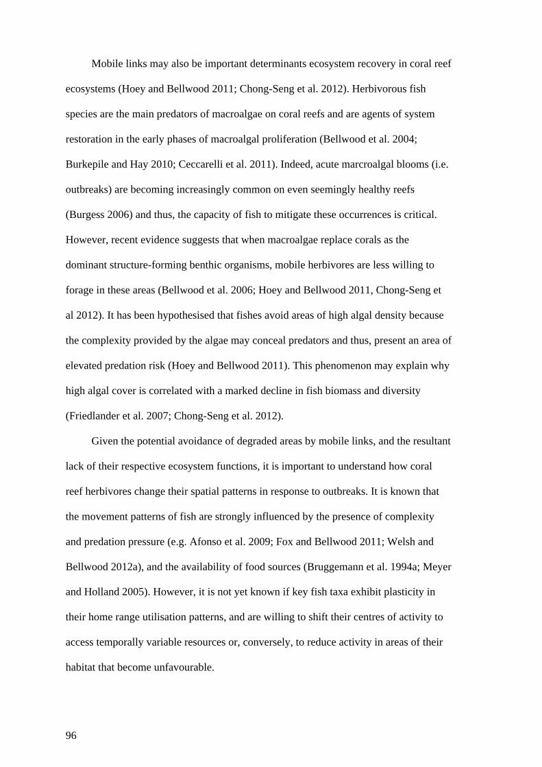
96
Mobile links may also be important determinants ecosystem recovery in coral reef
ecosystems (Hoey and Bellwood 2011; Chong-Seng et al. 2012). Herbivorous fish
species are the main predators of macroalgae on coral reefs and are agents of system
restoration in the early phases of macroalgal proliferation (Bellwood et al. 2004;
Burkepile and Hay 2010; Ceccarelli et al. 2011). Indeed, acute marcroalgal blooms (i.e.
outbreaks) are becoming increasingly common on even seemingly healthy reefs
(Burgess 2006) and thus, the capacity of fish to mitigate these occurrences is critical.
However, recent evidence suggests that when macroalgae replace corals as the
dominant structure-forming benthic organisms, mobile herbivores are less willing to
forage in these areas (Bellwood et al. 2006; Hoey and Bellwood 2011, Chong-Seng et
al 2012). It has been hypothesised that fishes avoid areas of high algal density because
the complexity provided by the algae may conceal predators and thus, present an area of
elevated predation risk (Hoey and Bellwood 2011). This phenomenon may explain why
high algal cover is correlated with a marked decline in fish biomass and diversity
(Friedlander et al. 2007; Chong-Seng et al. 2012).
Given the potential avoidance of degraded areas by mobile links, and the resultant
lack of their respective ecosystem functions, it is important to understand how coral
reef herbivores change their spatial patterns in response to outbreaks. It is known that
the movement patterns of fish are strongly influenced by the presence of complexity
and predation pressure (e.g. Afonso et al. 2009; Fox and Bellwood 2011; Welsh and
Bellwood 2012a), and the availability of food sources (Bruggemann et al. 1994a; Meyer
and Holland 2005). However, it is not yet known if key fish taxa exhibit plasticity in
their home range utilisation patterns, and are willing to shift their centres of activity to
access temporally variable resources or, conversely, to reduce activity in areas of their
habitat that become unfavourable.
97
The notion that the spatial tendencies of taxa can have a marked impact on the
recovery potential of ecosystems is troubling given the available evidence for coral
reefs. The scales over which herbivorous fish taxa operate appear, with only rare
exceptions, to be small, with site-attached behaviour being the most common (e.g.
Eristhee and Oxenford 2001; Meyer and Holland 2005; Welsh and Bellwood 2012a;
Brandl and Bellwood 2013). Moreover, our understanding of the response of herbivores
to the presence of algae on reefs is entirely limited to small-scale simulated outbreaks
(Hay 1981; Lewis 1985; Hoey and Bellwood 2011). Indeed, assessments of herbivore
predation of macroalgae on healthy reefs are overwhelmingly based on assays
comprised of a single thallus, or bunch of algae, and rarely exceed 1 m2 (e.g. Hoey and
Bellwood 2009; Rasher et al. 2013, but see Hughes et al. 2007; Burkepile and Hay
2010). These evaluations have identified several groups of herbivores with important
functions (croppers, scrapers and excavators which graze algae, and browsers which
consume adult macroalgae; Bellwood et al. 2004). Yet we know little of the behaviour
and spatial scales over which these key taxa operate, especially in response to
macroalgal outbreaks. Clearly larger-scale experimental manipulations are required to
understand how the spatial tendencies of local herbivores may change in response to
local algal outbreaks and to determine how reliant areas of reef are on the movement of
fishes from afar.
The aim of this study, therefore, is to evaluate changes in the spatial tendencies of
coral reef herbivores when exposed to an acute, large-scale simulated algal outbreak.
Specifically, we aim to determine if, and to what extent, the response of key fish taxa to
algal outbreaks is a localized one (i.e., the response of herbivorous taxa will be limited
to those taxa whose home range encompasses the outbreak) or a broader, community
level response (i.e., the response occurs over the entire reef and key species move in to
prey on macroalgae).
98
6.2 Materials and Methods
Study locations
The study was conducted between April and November 2013, on reefs surrounding
Lizard Island, a mid-shelf reef of the GBR (14o40’S 145o28’E). Two locations were
selected to conduct the experiment, Mermaid Cove and Turtle Beach (Appendix D).
Both locations are similar, on the leeward side of Lizard Island, with a distinct reef flat,
crest, slope and base on sand at 6-8 m. Data for video analysis occurred exclusively on
the reef crest (1-3 m) while algal deployment extended from the reef flat (0 m) to the
reef slope (5 m) at both locations (Fig. 6.1). At both study locations, macroalgae
naturally occurs in very low biomass (Wismer et al. 2009) and therefore, the algae had
to be collected from off-site.
Fig. 6.1 Visual representation of the simulated macroalgal outbreak depicting initial
macroalgal deployment density with acoustic receiver placement.
Algal treatment area
Receiver0 m
8 m
99
Simulated degradation
A degraded macroalgal-dominated reef was simulated by transferring Sargassum
sp. (cf. S. swartzii) from the Turtle Island group, an inshore group of reefs 27 km
southwest of Lizard Island (14°43’S, 145°12’E) to Lizard Island. Sargassum was
chosen for the simulation as it has been shown to be the dominant successional
macroalgal genus on the GBR (Hughes et al. 2007). Sargassum outbreaks have also
been reported from the Indian Ocean (Graham et al. 2006). Sargassum thalli of
relatively uniform height (~50 cm) were removed from the benthos by gently prying the
holdfast from the substratum. The algae were then transported to the Lizard Island
Research Station (LIRS) where they were held in flow through tanks before being
deployed. Algae were never held for more than a week and no algae were deployed
which showed signs of degradation. Prior to being deployed, algal thalli were spun,
weighted and attached together using twist ties to ensure that each deployed unit
weighted approximately 0.5 kg. To fix the algae to the reef, 6 m long chains were
placed in a grid configuration within a 50 m2 treatment area (algal plot), two days prior
to algal-treatment video data collection. Following the pre-deployment recording period
(see below for details) algae were attached to the chains using cable ties, which were
attached to the holdfast of the thallus.
Between October and November 2013, algae were fixed to the reef in a treatment
site within each location, measuring approximately 50 m2 (Fig. 6.1). The algal plot
extended 5 m along the reef and 10 m down the reef gradient, encompassing the reef
flat, crest and base. Initially, 200 thalli were deployed haphazardly within the algal plot
at each treatment site, resulting in an initial density of 4 thalli m-2 (approximately 2 kg
m-2). However, supplemental algae were added to each site every second day to
maintain densities of between 150-220 thalli per plot (density range; 3-4.4 thalli per m2;
100
1.5-2.2 kg m-2). At even the lowest algal density, sufficient Sargassum was present to
ensure that the macroalgal composition of the benthos was numerically dominant to
coral colony abundance. Algal plots were maintained on the reef for 14 days before
being removed.
Community response
To quantify the effect of an algal outbreak on the herbivore community, fishes were
monitored using cameras and acoustic telemetry. For video recordings, four monitoring
sites were chosen at each location. The monitoring sites roughly corresponded the
placement of VR2W acoustic receivers (Vemco, Halifax) moorings deployed along the
reef crest (details below). Cameras were placed to monitor a small-scale and large-scale
response. The small-scale response was assessed with two recording sites, one within
the algal treatment site, and the other (used to quantify changes in the herbivore
community in the immediate vicinity) was just outside the plot, 40 m away. Larger-
scale effects on the herbivore community were assessed using two supplementary
monitoring sites, roughly situated at acoustic receiver moorings 80 m along the reef on
either side of the central monitoring sites (Appendix D).
In total, 30 days of videos were captured over 34 days. Monitoring was divided
into three periods: ten pre-algal treatment days in October prior to algal deployment, ten
days when the ‘algal-treatment’ was present and finally, ten post-disturbance days
following algal removal. Video monitoring was suspended for two days prior to the
algal treatment and two days following the algal treatment to allow the community to
acclimate to the placement and removal (respectively) of the chains used to fix the
algae to the reef. Within each of these monitoring periods, five days were randomly
chosen for analysis. Video recordings were made using GoPro cameras, which were
haphazardly deployed onto the reef crest within 10 m of each monitoring site (4

101
cameras per location), between 11:00 h and 16:00 h. After each camera had been
deployed, a 1 m2 quadrat with markings at 5 cm intervals on all four sides was placed
50 cm from the lens of the camera for 30 s. This ensured that the video sampling area
was standardised and that size of fish that entered the sampling area could be estimated.
Each camera was then left for a minimum of 3.5 h. Videos were examined on a
computer with the sampling area marked on a plastic overlay on the screen. On the
overlay, the 5 cm increments placed on the sampling quadrate were also marked down
to aid in the accurate size estimation of the fish observed. Observer size estimations
were validated by holding a model of a size unknown to the observer within the
quadrate area. This was replicated 30 times. The estimated size of the model was then
compared to its actual size. The absolute discrepancy between actual size and observer
estimations was small (4.5 ± 0.49 cm; mean ± SE) and the relationship between
estimated and actual size of the model yielded an r2 value of 0.92.
In each video the identity, size and number of herbivorous fish species passing
through the sampling area in the videos were recorded for the second 15 min period in
each hour of recording, resulting in a total of 45 min per replicate. Fish abundance is
based on the number of individuals recorded over the 45 min period. As individuals
could not be reliably identified, the total number of appearances in the video is recorded
as an indication of herbivore presence.
Response of residents
The response of focal individuals to the localized algal outbreak was also quantified
using passive acoustic telemetry. In April 2013, two arrays of 10 VR2W acoustic
receivers were constructed at each location (total of 20 receivers). Prior to receiver
placement, extensive range testing was conducted at both study locations and the
102
working detection range (range at which 50% of known signal transmissions from a
transmitter are detected; Welsh et al. 2012a) was found to be 40 m for the V7-4L
acoustic transmitters (Vemco, Halifax) used in this study. Therefore, receivers were
placed at increments of 40 m along the reef crest at each location. At each location,
most of the reef crest was thus incorporated into the detection range of at least one
receiver. Receivers were moored following the shallow water moorings described in
Welsh et al. (2012) and care was taken to ensure that the hydrophone of each VR2W
unit was well above the algal canopy.
Once the array was in place, representative herbivore fish taxa were captured and
tagged between April and September 2012. Prior to tagging, visual censuses at each
location were used to estimate the average abundance of major herbivore species per
location. Visual censuses were conducted 5 times over five-months, prior to the study,
to ensure patterns of fish abundance were stable through time. At each location, a fish
census consisted of nine 2 x 20 m transects along the reef crest. The start-point of
transects were haphazardly chosen within 20 m of each receiver mooring. Based on
these data, representative individuals from herbivore functional groups that were likely
to respond to algal presence (browsers, scrapers and croppers) were selected for
tagging; these include Naso unicornis (browser), Scarus schlegeli (scraper), Siganus
vulpinus and S. corallinus (croppers) (Cheal et al. 2012).
Fish for acoustic tagging were captured using barrier nets. Once captured, fish
where transported to LIRS where they were held in flow-though tanks prior to surgery.
To implant transmitters, fish were anaesthetized in 70 L bath containing an MS-222
seawater solution (0.13 gL-1). Fish were considered anaesthetised when their righting
reflex failed and gilling rate became reduced, which took approximately 5 mins in the
anesthetic bath. The surgery was preformed in a relatively sterile environment, and the
fish were placed on a moist foam block, out of water, for the procedure. A small, 2 cm
103
incision was then made mid-way between the upper margin of the pectoral fin insertion
and the anus and a V7-4L acoustic transmitter inserted into the peritoneal cavity, below
the swim bladder. The wound was closed with two dissolvable BIOSYN 3/0 sutures,
tied using a Surgeon’s Knot. The surgical procedure took on average 180 (± 40)
seconds to complete once the fish had been removed from the anesthetic bath. Fish
were released following a 12-24 h recovery period to the capture location. Based on
visual observations of the tagged individuals, fish were fully recovered, showing no
signs of the incision, one week after being released.
Data analysis
Herbivore community response
The taxa observed in video data recordings were classified into functional groups
(grazers, scrapers, excavators and browsers; see Appendix D for species classification),
to examine the response of functional groups to the presence of macroalgae.
The abundance data for functional groups were compared using a three-way
MANOVA, in which Site, Location and Treatment were used as independent fixed
factors and Location was nested within Site. For this analysis, the numbers of
individuals from each functional group were used as dependant variables. Within the
MANOVA analysis, one-way ANOVA analyses were used to test the between-subject
effects, identifying which functional groups differed significantly between sites,
locations and algal treatments. Least significant differences analyses (LSD; based on
mean comparisons; t-test) were then used to detect homogeneous subsets of functional
group abundance in the independent factors. To satisfy the assumptions of the
MANOVA, abundance data were square-root transformed. Assessments of the square-
104
root transformed data revealed that the MANOVA was a suitable analysis based on a
non-significant Box’s test for equality of covariance matrices and a non-significant
Leven’s test for homogeneity. Residual plots were also inspected to verify the
suitability of the test.
To investigate species-level response of coral reef herbivores to macroalgae, non-
metric multidimensional scaling analyses (nMDS) were examined using video-based
based abundance data for each herbivore species (all herbivore species and non-
browsing species alone). In both cases, the significance of groupings identified in the
nMDS were analysed using a one-way analysis of similarity (ANOSIM) preformed on
an average distance matrix. Prior to nMDS and ANOSIM analyses, data were square-
root transformed to improve normality in the data set and reduce the influence of highly
abundant species on the analyses.
Resident response
To assess the response of tagged fish to the macroalgal disturbance, the detection data
from 14 days prior to, during and following the algal deployment were used (excluding
the two days during which algae was being deployed). For each fish an individual’s
core receiver (with the majority of an individual’s detections during the 14 days prior
the algal deployment) was identified. The change in occupancy at the core receiver was
calculated for each tagged individual by subtracting the average number of detection
per day prior to algal deployment from the average number of daily detections at the
same receiver while the algae were in place. The resulting delta values were then
compared to 0 (representing no change in occupancy) using four one-sample t-test (one
separate analysis per species). Furthermore, the activity of tagged fish within the
detection range of the receivers in the centre of each simulated algal outbreak
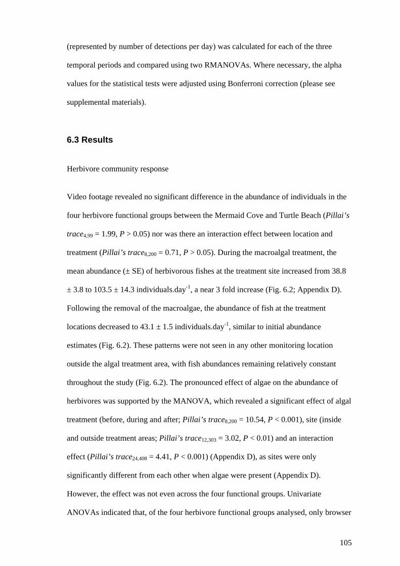
105
(represented by number of detections per day) was calculated for each of the three
temporal periods and compared using two RMANOVAs. Where necessary, the alpha
values for the statistical tests were adjusted using Bonferroni correction (please see
supplemental materials).
6.3 Results
Herbivore community response
Video footage revealed no significant difference in the abundance of individuals in the
four herbivore functional groups between the Mermaid Cove and Turtle Beach (Pillai’s
trace4,99 = 1.99, P > 0.05) nor was there an interaction effect between location and
treatment (Pillai’s trace8,200 = 0.71, P > 0.05). During the macroalgal treatment, the
mean abundance (± SE) of herbivorous fishes at the treatment site increased from 38.8
± 3.8 to 103.5 ± 14.3 individuals.day-1, a near 3 fold increase (Fig. 6.2; Appendix D).
Following the removal of the macroalgae, the abundance of fish at the treatment
locations decreased to 43.1 ± 1.5 individuals.day-1, similar to initial abundance
estimates (Fig. 6.2). These patterns were not seen in any other monitoring location
outside the algal treatment area, with fish abundances remaining relatively constant
throughout the study (Fig. 6.2). The pronounced effect of algae on the abundance of
herbivores was supported by the MANOVA, which revealed a significant effect of algal
treatment (before, during and after; Pillai’s trace8,200 = 10.54, P < 0.001), site (inside
and outside treatment areas; Pillai’s trace12,303 = 3.02, P < 0.01) and an interaction
effect (Pillai’s trace24,408 = 4.41, P < 0.001) (Appendix D), as sites were only
significantly different from each other when algae were present (Appendix D).
However, the effect was not even across the four functional groups. Univariate
ANOVAs indicated that, of the four herbivore functional groups analysed, only browser
106
densities changed significantly with algal treatments (F2,120 = 53.97, P < 0.001) and the
interaction effect (F6,120 = 25.37, P < 0.001) (i.e., as increases in browser abundance
only occurred at sites where and when algae were present)( Appendix D).
Algal removal during the simulated algal outbreak was significant. During the
period over which the algae were deployed, approximately 50 new thalli were added to
each site every second day to replace lost algal thalli. When removed, the holdfast of
the algal thalli were still present, and attached to the benthos, however, the standing
stipe and blades were all but removed. This suggested that thalli were not being lost as a
result of dislodgement but instead were being fed upon by herbivores in the
environment.
107
Fig. 6.2 The average abundance of a) total herbivore community and b) browsing
herbivore community before (white), during (black) and after (grey) a simulated phase
shift to macroalgae.
The size structure of the browser population also changed dramatically when
algae were placed on the reef. After deployment, there was more than a 10-fold increase
in the number of large N. unicornis, with an average of 33.2 ± 4.0 individuals recorded
per day over 30 cm when algae were present (Fig. 6.3). This pattern was even more
pronounced for K. vaigiensis and S. doliatus, in which the total number of individuals
increased in abundance at algal treatment sites by 4,900% (to 24.8 ± 3.1 individuals
recorded per treatment day) and 5,600% (to 26.0 ± 9.7 individuals recorded per
treatment day), respectively (Fig. 6.3). A smaller, yet still notable increase in abundance
by 470% was also found for K. cinerascens at sites of algal deployment (Fig. 6.3).
Brow
ser a
bund
ance
(mea
n ±
SE)
(a)
0
20
40
60
80
100
120
0
20
40
60
80
100
120(b)
0m 20m 80mDistance from phase shift
Her
bivo
re a
bund
ance
(mea
n ±
SE)

108
Fig. 6.3 Size frequency distribution of key browsing taxa; Kyphosus vaigiensis, Naso
unicornis, K. cinerascens and Siganus doliatus before (white), during (black) and
following (grey) a simulated phase shift to macroalgae.
K. vaigiensis
0
2
4
6
8
10
12
14
16
18
S. doliatus
0
2
4
6
8
10
12
14
16
18K. cinerascens
<10 10-20 20-30 >300
1
2
3
4
5
N. unicornis
Size class (cm)
Ave
rage
num
ber o
f ind
ivid
uals
(± S
E)
0
5
10
15
20
25
30
35
40
45
<10 10-20 20-30 >30 <10 10-20 20-30 >30
<10 10-20 20-30 >30
Pre algal deploymentAlgal deploymentPost algal deployment
109
The results from the species-level MDS analysis support the above observations
with a strong separation of sites during algal deployment (Fig. 6.4). ANOSIM detects a
significant difference between samples in which algae were present and all others
(global R = 0.937, significance level 0.1%; Fig. 6.4). As expected, the separation of
these sites was largely driven by the presence of browsing species, namely Naso
unicornis, Kyphosus vaigiensis, Siganus doliatus, and to a lesser extent, K. cinerascens
(Fig. 6.4). When all browsers were removed from the data set, no significant groupings
were detected (global R = -0.125, significance level 89.2%)(Appendix D).
Resident response
A total of 34 fish tagged with acoustic transmitters were monitored for the duration of
the study. The number of each species tagged (S. vulpinus n = 6, S. corallinus n = 6,
Scarus schlegeli n = 17 and N. unicornis n = 3) corresponded to the relative abundance
of the taxa at each site and represented at least 40% of the estimated local population
size (based on counts made during fish censuses; Appendix D). Despite the marked
changes in herbivore detections observed by videos, of the tagged fishes, none
significantly changed their patterns of occupancy during algal deployment, regardless
of whether their core area of detection encompassed the simulated algal outbreak or not
(Fig. 6.5; Appendix D).
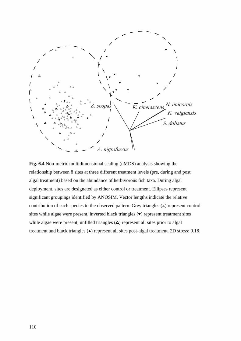
110
Fig. 6.4 Non-metric multidimensional scaling (nMDS) analysis showing the
relationship between 8 sites at three different treatment levels (pre, during and post
algal treatment) based on the abundance of herbivorous fish taxa. During algal
deployment, sites are designated as either control or treatment. Ellipses represent
significant groupings identified by ANOSIM. Vector lengths indicate the relative
contribution of each species to the observed pattern. Grey triangles ( ) represent control
sites while algae were present, inverted black triangles ( ) represent treatment sites
while algae were present, unfilled triangles ( ) represent all sites prior to algal
treatment and black triangles ( ) represent all sites post-algal treatment. 2D stress: 0.18.
K. cinerascensK. vaigiensis
N. unicornis
S. doliatus
Z. scopas
A. nigrofuscus
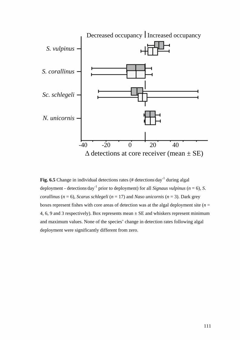
111
Fig. 6.5 Change in individual detections rates (# detections.day-1 during algal
deployment - detections.day-1 prior to deployment) for all Signaus vulpinus (n = 6), S.
corallinus (n = 6), Scarus schlegeli (n = 17) and Naso unicornis (n = 3). Dark grey
boxes represent fishes with core areas of detection was at the algal deployment site (n =
4, 6, 9 and 3 respectively). Box represents mean ± SE and whiskers represent minimum
and maximum values. None of the species’ change in detection rates following algal
deployment were significantly different from zero.
0-20-40 20 40
N. unicornis
Sc. schlegeli
S. corallinus
S. vulpinus
Decreased occupancy Increased occupancy
Δ detections at core receiver (mean ± SE)
112
6.4 Discussion
Following a simulated outbreak of macroalgae the herbivorous fish community
exhibited a rapid, positive, response. This activity was highly focused, with no other
areas on the same reef, even within 20 m, exhibiting similar increases in herbivore
abundance. The observed increase in fish abundance, however, did not arise from a
response in resident taxa. Instead, it occurred as large mobile non-resident herbivores
moved in to the site of algal deployment to feed on the available macroalgae. It appears
that large mobile browsing herbivores can alter their behaviour to occupy areas
exhibiting a localized algal outbreak. These observations suggest that coral reefs may
rely on the activities of mobile links, i.e. large, mobile, non-resident individuals, to
mitigate the effects of localized algal outbreaks on coral reefs.
A community response to algal outbreaks
The response of the fish community to the simulated macroalgal outbreak was
marked. On average, the fish abundance at the site of algal deployment increased by
267%. This response was surprising, as several studies have evaluated the effect of
macroalgal growth on coral reefs and have overwhelmingly found a decline in fish
abundance and/or diversity (McClanahan et al. 1999; Wilson et al. 2008; Chong-Seng
et al. 2012). The cause for these declines has largely been attributed to a decline in reef
complexity or suitable feeding surfaces following a phase-shift over long temporal
scales (Graham et al. 2006; Chong-Seng et al. 2012), or the proliferation of undesirable
complexity provided by macro-algae (Hoey and Bellwood 2011). However, we found
that for localized, acute increases in algae where the reef structure remains intact, the
overall herbivore community shows no aversion to macroalgae; instead, large browsers
exhibit a strong attraction to its location.
113
There are two possible explanations for these differences among studies
evaluating acute algal deployments on coral reefs: 1) they may be a result of differences
in algal identity, density, quality and/or extent, or 2) variation among studies in the
composition of the herbivore assemblages. Previous work that has shown an aversion to
large stands of macroalgae (Bellwood et al. 2006) may in part be due to algal densities
that were higher than those in the present study. This suggests that there is a threshold
above which algal densities elicit a negative herbivore response and algal outbreak
removal becomes difficult (Bellwood et al. 2006; Hoey and Bellwood 2011).
Alternatively algae may differ in palatability where larger, older thalli are less desirable
to herbivores (Bellwood et al. 2006; Hoey 2010; Lefèvre and Bellwood 2010), reducing
the likelihood of herbivores responding to algal presence on reefs. Fish assemblage
structure may also be important. The present study is the first on a mid-shelf reef, where
the higher fish diversity provides a greater potential a range of species to respond to
algal deployments. Furthermore, macroalgae are rare on mid-shelf reefs relative to
inner-shelf reefs (Wismer et al. 2009). Therefore, browsing herbivores may be more
willing to feed on high density macroalgae on mid-shelf reefs, as the benefits of
accessing the rare resource outweigh the elevated predation risks that may be associated
with dense algal fields (Hoey and Bellwood 2011).
The observed increase in total fish abundance was driven almost entirely by large
macroalgal browsers. When algae were present we recorded abundances of the
browsing species, N. unicornis, up to 10 times higher than in either pre- or post-
monitoring periods and a similar, yet less marked increase in the abundance of K.
vaigiensis was recorded. These species are know to feed primarily on macroalgae
(Choat et al. 2002) and have been found to be uniquely capable of removing large
quantities of macroalgae on the great barrier reef (Cvitanovic and Bellwood 2009; Hoey
and Bellwood 2009) and elsewhere in Australia (Vergés et al. 2011). This demonstrated
114
a localized accumulation of functionally important taxa with the ability to reverse local
algal outbreaks. Studies from the Seychelles (Chong-Seng et al. 2012) and the Red Sea
(Khalil et al. 2013) found a similar trend, in which degraded reefs with algal
proliferation supported a higher abundance of browsing herbivorous taxa, as individuals
presumably move in to feed on outbreaks of algae. While movement of taxa for the
purposes of resource exploitation is not a rare phenomenon in terrestrial or pelagic
ecosystems (e.g. Polovina 1996; Pomilla and Rosenbaum 2005; McKinney et al. 2012),
where large-scale movements are common, movements of this kind for the purpose of
resource exploitation have not yet been recorded coral reefs. It appears that mobile fish
taxa are capable of concentrating their residency and foraging activities at the site of
macroalgal outbreaks in the same way terrestrial taxa change their behaviour to exploit
specific resources. However, this raises the question of where did the individuals
responsible for the increase in browser abundance come from?
The origin of responders
One of the most remarkable observations was that the increase in browsers was
not a result of the movement of local residents. Of the three resident N. unicornis and
29 other herbivores tagged, none moved. The lack of response from the resident
community is also supported by the distinct shift in the size-frequency distribution of
the browsing taxa. We recorded a clear peak in the number of large individuals (> 30
cm), which were, in the case of N. unicornis, not recorded on the reef prior to the algal
deployment. A similar pattern was found for K. vaigiensis, K. cinerascens and S.
doliatus in which the number of large individuals was greater than the combined daily
counts for these taxa across all sites prior to algae deployment. Indeed, K. vaigiensis
was only recorded twice on the reef prior to the algal deployment in data from both
115
video recordings and visual census. The dramatic increase in browser abundance, and
subsequent decline following algal removal, was recorded at both sites and arose from
an influx of non-resident individuals that exhibited home ranges of a sufficient
magnitude to allow them to encounter the algae.
Large-scale movements have been documented previously for K. vaigiensis on
inshore reefs. Welsh and Bellwood (2014) recorded movements in K. vaigiensis that
were unprecedented for a coral reef herbivore and speculated that these movements
may facilitate the locating of food sources with a patchy distribution. This study
supports this hypothesis and demonstrates the ability of these highly vagile taxa to
change their movements in response to food availability. In contrast, the lack of
movement in the smaller local fish is consistent with number recent studies, which
report limited home ranges (Eristhee and Oxenford 2010; Meyer and Holland 2005;
Fox and Bellwood 2011; Welsh and Bellwood 2012a). This site-attached behaviour in
reef fish highlights the importance of those species that do exhibit a spatial response.
It appears that upon prey detection, large browsing herbivores can quickly alter
their spatial range to exploit areas of high food availability. Previous research has
suggested that N. unicornis is a highly site attached species with a restricted home range
(Meyer and Holland 2005; Marshell et al. 2011). However, studies on this species’
movements are often restricted to small individuals although ontogenetic home range
expansions have been documented (Marshell et al. 2011). The present observations are,
again, consistent with these previous studies where smaller, resident N. unicornis do not
move far, but larger individuals exhibit far greater mobility.
Once the macroalgae were removed, the abundance of browsing taxa returned to
abundances almost indistinguishable from those before the simulated phase shift. This
suggests that the browsers did not shift their home range to a new location in favour of
a new resource but instead, temporarily changed their core-areas of utilization within a

116
much larger spatial range. This is significant, as it would suggest that the plasticity of
movements within an individual’s home range might be key to preventing algal
establishment and proliferation on coral reefs over large spatial scales, and may
supplement the small-scale functional processes on reefs conferred by resident taxa.
The importance of mobile links on coral reefs
The response of the mobile browsing herbivore community to the presence of
macroalgae may be an important line of defence against reef phase- or regime shifts. In
this study, I present evidence that the large-scale movements of roving browsing
herbivores may be significant in preventing long-term macroalgal outbreaks on coral
reefs. Resident taxa alone may be unable to control algal outbreaks. It has been
suggested that the growth rate of Sargassum may be too great for the algae to be
removed entirely by resident taxa, and once established, fish may be unwilling to prey
on the macroalgae (Hoey and Bellwood 2011). Moreover, even on a small scale, the
site-attached nature of numerous reef taxa is such that, even if an outbreak occurs on
their reef, they may never encounter it (Nash et al. 2013). Large, mobile herbivores may
act as key mobile links, safeguarding against algal outbreaks, providing a broad-scale
application of functional processes, with sufficient plasticity in their movements to
focus their ecosystem services where needed.
This ecosystem response, however, is reliant on a healthy herbivore community,
with large browsing individuals remaining in the system. In particular it is not just
species or adult individuals that are needed but large, mobile, individuals. This is
especially concerning given that these large, mobile taxa are highly coveted by
fishermen and among the first to be removed from a system when fishing intensity
increases (Hoey and Bellwood 2009; Moffitt et al. 2009; Nash et al. 2013; Bejarano et
al. 2013). Furthermore, most MPAs are small, especially in tropical developing nations,

117
where reef fish are highly targeted as a primary food source (Wood et al. 2008).
Therefore, by virtue of their mobility, these highly important individuals and species
are more likely to diffuse out of MPA boundaries and be removed first from the system.
Fish that act as mobile links, therefore, appear to be some of the most important yet
vulnerable organisms on coral reefs.
118
Chapter 7: Concluding Discussion
The movements of animals are of particular importance for our understanding of
ecosystems, as the spatial ecology of organisms delineates their functional impact (Fox
and Bellwood 2011; Welsh and Bellwood 2012a). Thus, there has been a recent
emphasis on the study of spatial aspects of a species’ biology. Although this field is still
in its infancy, the last decade has seen a rapid expansion in the number of studies that
quantify animal movements, specifically those of marine taxa (Welsh and Bellwood
2014; Nash et al. in review). The majority of studies into the spatial utilization patterns
of marine taxa, especially taxa on coral reefs, have focused on quantifying the
effectiveness of MPAs and the survivorship of individuals (Meyer et al. 2010; Claisse
et al. 2011; Maypa et al. 2012; Calò et al. 2013). This thesis represents a contrasting
view, to explore the ecological implications of movement, and to examine the functions
of coral reef fishes in a spatial context.
Acoustic telemetry; an evolving frontier
Methods for quantifying the movements of marine taxa have traditionally lagged
behind those of terrestrial species (Lacroix and Voegeli 2000; Simpfendorfer et al.
2008; Mathies et al. 2014). This is largely due to the logistical difficulties of tracking
movements in the marine environment (Heupel et al. 2006, 2008; Welsh et al. 2012). In
the past two decades, however, the refinement of acoustic technology has facilitated a
rapid expansion in the number, kind and quality of spatial studies in the marine
environment (Kerwath et al. 2005; Holland et al. 2009; Biesinger et al. 2013). Yet,
movement studies on adult coral reef organisms have received comparably less
119
attention than those inhabiting temperate or pelagic systems. This is, yet again,
attributable to the difficulties of using acoustic telemetry on structurally complex reefs
(Biesinger et al. 2013; Mathies et al. 2014). Given the threats facing coral reefs and the
need for new questions to be answered regarding their functioning and how best
conserve them, a growing body of empirical studies and new analysis programs are
overcoming the difficulties of utilizing acoustic telemetry on reefs (Cagua et al. 2013;
Mathies et al. 2014). Chapter 2 of this thesis is one such study and provided among the
first empirical data and framework to facilitate the expansion of acoustic studies on
coral reefs. These have now opened up this environment to be studied in greater detail
than was previously possible, and there are now fewer logistical constraints on
ecological studies involving animal movements on coral reefs. With a growing
understanding of the complications associated with the use of telemetry in coral reef
environments, such as those outlined in chapter 2, future studies may account for the
unique complexities and ultimately, conduct more detailed evaluations of reef fish
movements.
Spatial ecology
In conjunction with advancements in spatial data analyses, available data on the
movements of marine taxa has dramatically expanded. Acoustics telemetry has leaded
this expansion, with refinements to the technology increasing the number of species that
can be studied using internal transmitter implantation and subsequent tracking (Fig.
1.1). As a result, there is now a growing body of robust, empirical studies that present
data on the range size of coral reef fishes (e.g. Meyer and Holland 2005; Hutchinson
and Rhodes 2010; Fox and Bellwood 2011, Welsh and Bellwood 2012a, b; Welsh and
Bellwood 2014).
120
Overexploitation is among the greatest threats to reef fish populations, and
indeed, their declines have been recorded from around the globe (Wood et al. 2008). As
a result, conservation initiatives are being informed by numerous studies, which analyse
movement patterns of reef fishes (Bennett et al. 2012). These data are being used with
the goal of quantifying the effectiveness of MPAs, to conserve marine populations.
Separately, the interaction between marine taxa and their environment are among the
topics in the forefront of ecological research, as ecosystem degradation is another factor
that continues to threaten coral reefs (Bellwood et al. 2006; Hughes et al. 2007). Thus,
several studies have endeavoured to quantify the impact of key taxa on their
environment. By combining these types of research, and incorporating movement
studies into the evaluation of ecological processes, it is possible to better understand the
ecology of coral reef ecosystems and gain spatially explicit view of coral reef functional
processes. This thesis stands as an example of this. In using acoustic telemetry, spatial
data and ecological data in concert, key questions ecological questions that have never
before been able to be addressed have been answered. This has broadened our
understanding of the underlying variability in functional processes, and highlighted the
importance of considering the spatial resilience of ecosystems. With this knowledge,
future studies may consider the incorporation of key species’ spatial ecology as a key
element in determining taxa’s importance for ecological process.
Among the challenges associated with quantifying movements in the marine
environment is to understand which factors shape and/or limit the home range of an
individual. At present, limitations to an individual’s home range size have largely been
attributed to both physical barriers, such as habitat discontinuity (e.g. Bakker and van
Vuren 2004; Afonso et al. 2009; Downie et al. 2013; José et al. 2013) and unfavourable
substratum (Hoey and Bellwood 2011), as well as social restrictions, i.e. the boundaries
of a social group’s territory (Bruggemann et al. 1994b; Mumby and Wabnitz 2002;
121
Welsh and Bellwood 2012a; Welsh et al. 2013). Despite a growing body of research on
the topic, no consensus has yet to produced and indeed, the mechanisms may vary
heavily between taxa, or even within taxa depending on ontogenetic development.
Despite this, the evidence presented herein strongly suggests that factors limiting the
movements of fishes play an important role in the spatial applications of functional
processes. Further research on the topic may provide invaluable information for our
understanding of the variability associated with quantifying the rate of ecosystem
functions, as well the effectiveness of marine reserves.
Regardless of the factors that limit home range boundaries in fishes, it is a
sobering notion that the home range areas of functionally important fishes are often
limited to a small area within a reef (Chapter 5; Welsh and Bellwood 2014). However,
the exact scale of movement associated with ‘roving’ behaviour appears to be
ambiguous. Indeed, evidence of roving behaviour in reef fishes has been limited, with
largely invariable reports of site-attached home ranging behaviour for herbivorous
species (e.g. Meyer and Holland 2005; Fox and Bellwood 2011; Marshell et al. 2011).
Concluding remarks
Previous evaluations of the ecosystem processes that occur on coral reefs, and other
ecosystems, have been largely processes-centric (e.g. Fox and Bellwood 2007;
Burkepile and Hay 2010; Vergés et al. 2011). As a result, the rates at which ecosystem
processes are applied are well documented and a detailed understanding of the
processes themselves has been established. However, estimates of the rate at which a
functional process is applied are often subject to a great deal of variability, in both
space and time (e.g. Bennett and Bellwood 2011; Lefèvre and Bellwood 2011). By
incorporating an understanding of the movements and spatial habits of the taxa that

122
drive ecological processes, it may be possible to better understand dynamics in these
processes. In doing this, we can theoretically track seasonal shifts in home range
patterns of a key herbivorous species to predict where algae will be removed from a
reef, or seeds may be dispersed through an ecosystem by a bird or bat. Moreover,
utilization frequency data for a species in a given area can be used to predict the
intensity at which a process may occur in that environment (Welsh and Bellwood
2012a). Put simply, it is perhaps by understanding the spatial biology of some of the
smallest units of functional processes, the individuals that drive them, that we may gain
a broader understanding of processes occurring in today’s ecosystems.
123
References
Afonso P, Fontes J, Holland KN, Santos RS (2008) Social status determines behaviour
and habitat usage in a temperate parrotfish: implications for marine reserve
design. Mar Ecol Prog Ser 359:215-227
Afonso P, Fontes J, Holland KN, Santos RS (2009) Multi-scale patterns of habitat use
in a highly mobile reef fish, the white trevally Pseudocaranx dentex, and their
implications for marine reserve design. Mar Ecol Prog Ser 381:273-286
Alevizon WS (1976) Mixed schooling and its possible significance in a tropical western
Atlantic parrotfish and surgeonfish. Copeia 1976:796-798
Allen GR, Steene RC, Humann P, Deloach N (2003) Reef fish identification - tropical
pacific. New World Publications, Jacksonville, FL
Almany GR, Webster MS (2006) The predation gauntlet: early post-settlement
mortality in reef fishes. Coral Reefs 25:19-22
Almany GR, Connolly SR, Heath DD, Hogan JD, Jones GP, McCook LJ, Mills M,
Pressey RL, Williamson DH (2009) Connectivity, biodiversity conservation and
the design of marine reserve networks for coral reefs. Coral Reefs 28:339-351
Alwany MA, Thaler E, Stachowitsch M (2009) Parrotfish bioerosion on Egyptian Red
Sea reefs. J Exp Mar Biol Ecol 371:170-176
Au WW, Banks K (1998) The acoustics of the snapping shrimp Synalpheus
parneomeris in Kaneohe Bay. J Acoust Soc Am 103:41-47
Avgar T, Mosser A, Brown GS, Fryxell JM (2013) Environmental and individual
drivers of animal movement patterns across a wide geographical gradient. J
Anim Ecol 82:96-106
Bakker VJ, van Vuren DH (2004) Gap-crossing decisions by the Red Squirrel, a forest-
dependent small mammal. Conserv Biol 18:689-697
124
Bardyshev VI (2007) Underwater ambient noise in shallow-water areas of the Indian
Ocean within the tropical zone. Acoust Phys 53:167-171
Bates, D.M. & Maechler, M. (2009) lme4: Linear mixed-effects models using S4
classes.
Bellwood DR (1988) Ontogenetic changes in the diet of early post-settlement Scarus
species (Pisces: Scaridae). J Fish Biol 33:213-219
Bellwood DR, Choat JH (1989) A description of the juvenile phase colour patterns of
24 parrotfish species (family Scaridae) from the Great Barrier Reef, Australia.
Aust Mus 41:1-41
Bellwood DR, Choat JH (1990) A functional analysis of grazing in parrotfishes (family
Scaridae): the ecological implications. Environ Biol Fish 28:189-214
Bellwood DR, Hoey AS, Choat JH (2003) Limited functional redundancy in high
diversity systems: resilience and ecosystem function on coral. Ecol Lett 6:281-
285
Bellwood DR, Hughes TP, Hoey AS (2006) Sleeping functional group drives coral-reef
recovery. Curr Biol 16:2434-2439
Bellwood DR, Hoey AS, Hughes TP (2012) Human activity selectively impacts the
ecosystem roles of parrotfishes on coral reefs. Proc R Soc B 279:1621-1629
Bellwood DR, Hughes TP, Folke C, Nyström M (2004) Confronting the coral reef
crisis. Nature 429:827-833
Bejarano S, Golbuu Y, Sapolu T, Mumby PJ (2013) Ecological risk and the exploitation
of herbivorous reef fish across Micronesia. Mar Ecol Prog Ser 482:197-215
Bennett S, Bellwood DR (2011) Latitudinal variation in macroalgal consumption by
fishes on the Great Barrier Reef. Mar Ecol Prog Ser 426:241-252
Bennett RH, Cowley PD, Childs A-R, Whitfield AK (2012) Area-use patterns and diel
movements of white steenbras Lithognathus lithognathus in a temporarily
125
open/closed South African estuary, inferred from acoustic telemetry and long-
term seine-netting data. Afr J Mar Sci 34:81-91
Berger J (2004) The last mile: How to sustain long-distance migration in mammals.
Conserv Biol 18:320-331
Biesinger Z, Bolker BM, Marcinek D, Grothues TM, Dobarro JA, Lindberg WJ (2013)
Testing an autonomous acoustic telemetry positioning system for fine-scale
space use in marine animals. J Exp Mar Biol Ecol 448:46-56
Bolden SK (2001) Using ultrasonic telemetry to determine home range of a coral-reef
fish. In: Sibert JR, Nielsen JL (eds) Electronic tagging and tracking in marine
fisheries. Kluwer Academic Publishers, Netherlands,
Bonaldo RM, Bellwood DR (2008) Size-dependent variation in the functional role of
the parrotfish Scarus rivulatus on the Great Barrier Reef, Australia. Mar Ecol
Prog Ser 360:237-244
Bonaldo RM, Krajewski JP (2008) Differences in interspecific associations of initial
and terminal phase parrotfish in north-eastern Brazil. Mar Biodivers Rec 1:e87
Bonaldo RM, Bellwood DR (2010) Spatial variation in the effects of grazing on
epilithic algal turfs on the Great Barrier Reef, Australia. Coral Reefs 30:381-390
Bonaldo RM, Welsh JQ, Bellwood DR (2012) Spatial and temporal variation in coral
predation by parrotfishes on the GBR: evidence from an inshore reef. Coral
Reefs 31:263-272
Bonaldo RM, Krajewski JP, Sazima C, Sazima I (2006) Foraging activity and resource
use by three parrotfish species at Fernando de Noronha Archipelago, tropical
West Atlantic. Mar Biol 149:423-433
Booth DJ, Beretta GA (2004) Influence of recruit condition on food competition and
predation risk in a coral reef fish. Oecologia 140:289-294
126
Börger L, Dalziel BD, Fryxell JM (2008) Are there general mechanisms of animal
home range behaviour? A review and prospects for future research. Ecol Lett
11:637-650
Brandl SJ, Bellwood DR (2013) Pair formation in the herbivorous rabbitfish Siganus
doliatus. J Fish Biol 82:2031-2044
Broomhall LS, Mills MGL, du Toit JT (2003) Home range and habitat use by cheetahs
(Acinonyx jubatus) in the Kruger National Park. J Zool 261:119-128
Brown JL (1975) The evolution of behaviour. Norton, New York
Brown GP, Brooks RJ (1993) Sexual and seasonal differences in activity in a northern
population of snapping turtles, Chelydra serpentine. Herpetologica 49:311-318
Bruggemann HJ, Kuyper MWM, Breeman AM (1994a) Comparative analysis of
foraging and habitat use by the sympatric Caribbean parrotfish Scarus vetula
and Sparisoma viride. Mar Ecol Prog Ser 112:51-66
Bruggemann HJ, van Oppen MJH, Breeman AM (1994b) Foraging by the stoplight
parrotfish Sparisoma viride. I. Food selection in different, socially determined
habitats. Mar Ecol Prog Ser 106:41-55
Bruggemann JH, van Rooij MJ, Videler JJ, Breeman AM (1995) Dynamic and
limitations of herbivore populations on a Caribbean coral reef. Ph.D. thesis,
University of Groningen, pp 153-190
Bryars S, Rogers P, Huveneers C, Payne NL, Smith I, McDonald B (2012) Small home
range in southern Australia’s largest resident reef fish, the western blue groper
(Achoerodus gouldii): implications for adequacy of no-take marine protected
areas. Mar Freshw Res 63:552-563
Burgess SC (2006) Algal blooms on coral reefs with low anthropogenic impact in the
Great Barrier Reef. Coral Reefs 25:390-390

127
Burkepile DE, Hay ME (2008) Herbivore species richness and feeding complementarity
affect community structure and function on a coral reef. Proc Natl Acad Sci U S
A 105:16201-16206
Burkepile DE, Hay ME (2010) Impact of herbivore identity on algal succession and
coral growth on a Caribbean reef. PLoS ONE 5:e8963
Cagnacci F, Boitani L, Powell RA, Boyce MS (2010) Animal ecology meets GPS-
based radiotelemetry: a perfect storm of opportunities and challenges. Phil Trans
R Soc B 365:2157-2162
Cagua EF, Berumen ML, Tyler E (2013) Topography and biological noise determine
acoustic detectability on coral reefs. Coral reefs 32:1123-1134
Calenge C (2006) The package adehabitat for the R software: a tool for the analysis of
space and habitat use by animals. Ecol Model 197:516-519
Calò A, Félix-Hackradt FC, Garcia J, Hackradt CW, Rocklin D, Otón JT, Charton JAG
(2013) A review of methods to assess connectivity and dispersal between fish
populations in the Mediterranean Sea. Adv Oceanogr Limnol 4:150-175
Carbone C, Pettorelli N, Stephens PA (2011) The bigger they come, they harder they
fall: body size and prey abundance influence predator-prey ratios. Biol Lett
7:312-315
Carpenter R, Bennett EM, Peterson GD (2006) Scenarios for ecosystem services: an
overview. Ecol Soc 11:29-43
Cato DH (1978) Marine biological choruses observed in tropical waters near Australia.
J Acoust Soc Am 64:736-743
Ceccarelli DM, Jones GP, McCook LJ (2011) Interactions between herbivorous fish
guilds and their influence on algal succession on a coastal coral reef. J Exp Mar
Biol Ecol 399:60-67

128
Chapman MR, Kramer DL (2000) Movements of fishes within and among fringing
coral reefs in Barbados. Environ Biol Fish 57:11-24
Cheal A, Emslie M, Miller I, Sweatman H (2012) The distribution of herbivorous fishes
on the Great Barrier Reef. Mar Biol 159:1143-1154
Cheal AJ, Aaron MacNeil M, Cripps E, Emslie MJ, Jonker M, Schaffelke B, Sweatman
HPA (2010) Coral-macroalgal phase shifts or reef resilience: links with diversity
and functional roles of herbivorous fishes on the Great Barrier Reef. Coral Reefs
29:1005-1015
Chen LS (2002) Post-settlement diet shift of Chlorurus sordidus and Scarus schlegeli
(Pisces: Scaridae). Zool Stud 41:47-58
Choat J, Robertson D (1975) Protogynous hermaphroditism in fishes of the family
Scaridae Intersexuality in the animal kingdom. Springer, pp263-283
Choat JH, Bellwood DR (1985) Interactions amongst herbivorous fishes on a coral reef:
influence of spatial variation. Mar Biol 89:221-234
Choat JH, Clements KD, Robbins WD (2002) The trophic status of herbivorous fishes
on coral reefs. Mar Biol 140: 613-623.
Choat JH, Robbins WD, Clements KD (2004) The trophic status of herbivorous fishes
on coral reefs. Mar Biol 145:445-454
Chong-Seng KM, Mannering TD, Pratchett MS, Bellwood DR, Graham NAJ (2012)
The influence of coral reef benthic condition on associated fish assemblages.
PLoS ONE 7:e42167
Cinner JE, Graham NAJ, Hutchery C, MacNeil M (2012) Global effects of local human
population density and distance to markets on the condition of coral reef
fisheries. Conserv Biol 27:453-458
Claisse J, Clark T, Schumacher B, McTee S, Bushnell M, Callan C, Laidley C, Parrish J
(2011) Conventional tagging and acoustic telemetry of a small surgeonfish,
129
Zebrasoma flavescens, in a structurally complex coral reef environment.
Environ Biol Fish 91:185-201
Clements S, Jepsen D, Karnowski M (2005) Optimization of an acoustic telemetry
array for detecting transmitter-implanted fish. N Am J Fish Manag 25:429-436
Clifton KE (1989) Territory sharing by the Caribbean striped parrotfish, Scarus iserti:
patterns of resource abundance, group size and behaviour. Anim Behav 37:90-
103
Clutton-Brock TH, Hodge SJ, Flower TP (2008) Group size and the suppression of
subordinate reproduction in Kalahari meerkats. Anim Behav 76:689-700
Connell J (1997) Disturbance and recovery of coral assemblages. Coral Reefs 16:S101-
S113
Cooke SJ, Hinch SG, Wikelski M, Andrews RD, Kuchel LJ, Wolcott TG, Butler PJ
(2004) Biotelemetry: a mechanistic approach to ecology. Trends Ecol Evol
19:334-343
Couvreur M, Christiaen B, Verheyen K, Hermy M (2004) Large herbivores as mobile
links between isolated nature reserves through adhesive seed dispersal. Appl
Veg Sci 7:229-236
Cowman PF, Bellwood DR (2011) Coral reefs as cryptic extinction events, and the
development of biodiversity hotspots. J Evol Biol 24:2543-2562
Cox PA, Elmqvist T, Pierson ED, Rainey WE (1991) Flying foxes as strong interactors
in South Pacific island ecosystems: A conservation hypothesis. Conserv Biol
5:448-454
Cvitanovic C, Bellwood DR (2009) Local variation in herbivore feeding activity on an
inshore reef of the Great Barrier Reef. Coral Reefs 28:127-133
Depczynski M, Bellwood DR (2003) The role of cryptobenthic reef fishes in coral reef
trophodynamics. Mar Ecol Prog Ser 256:183-191
130
Depczynski M, Bellwood DR (2004) Microhabitat utilisation patterns in cryptobenthic
coral reef fish communities. Mar Biol 145:455-463
Depczynski M, Bellwood DR (2005) Shortest recorded vertebrate lifespan found in a
coral reef fish. Curr Biol 15:R288-R289
Downie RA, Babcock RC, Thomson DP, Vanderklift MA (2013) Density of
herbivorous fish and intensity of herbivory are influenced by proximity to coral
reefs. Mar Ecol Prog Ser 482:217-225
Dudgeon SR, Aronson RB, Bruno JF, Precht WF (2010) Phase shifts and stable states
on coral reefs. Mar Ecol Prog Ser 413:201-216
Duncan RS, Chapman CA (1999) Seed dispersal and potential forest succession in
abandoned agriculture in tropical Africa. Ecol Appl 9:998-1008
Egli DP, Babcock RC (2004) Ultrasonic tracking reveals multiple behavioural modes of
snapper (Pagrus auratus) in a temperate no-take marine reserve. ICES J Mar Sci
61:1137-1143
Elmqvist T, Maltby E. 2010. Biodiversity, ecosystems and ecosystem services. In:
Kumar P (ed) The economics of ecosystems and biodiversity: ecological and
economic foundations. Earthscan, Oxford, UK, pp 41–111.
Eloff PFC (1959) Observations on the migration and habits of the Antelopes of the
Kalahari Gemsbok Park - Part II
Eristhee N, Oxenford HA (2001) Home range size and use of space by Bermuda chub
Kyphosus sectatrix (L.) in two marine reserves in the Soufrière Marine
Management Area, St Lucia, West Indies. J Fish Biol 59:129-151
Evans MC (2008) Home range, burrow-use and activity patterns in common wombats
(Vombatus ursinus). Wildl Res 35:455-462

131
Ferreira CEL, Gonçalves JEA (2006) Community structure and diet of roving
herbivorous reef fishes in the Abrolhos Archipelago, southwestern Atlantic. J
Fish Biol 69:1533-1551
Fish MP (1964) Biological sources of sustained ambient sea noise. In: Tavolga WN
(ed) Marine bio-acoustics. Pergamon Press, New York, pp 175-194
Floeter SR, Ferreira CEL, Dominici-Arosemena A, Zalmon IR (2004) Latitudinal
gradients in Atlantic reef fish communities: trophic structure and spatial use
patterns. J Fish Biol 64:1680-1699
Folke C, Carpenter S, Walker B, Scheffer M, Elmqvist T, Gunderson L, Holling CS
(2004) Regime shifts, resilience, and biodiversity in ecosystem management.
Annual Review of Ecology Evolution and Systematics 35:557-581
Foster SA (1985) Group foraging by a coral reef fish: a mechanism for gaining access
to defended resources. Anim Behav 33:782-792
Fox RJ, Bellwood DR (2007) Quantifying herbivory across a coral reef depth gradient.
Mar Ecol Prog Ser 339:49-59
Fox RJ, Bellwood DR (2011) Unconstrained by the clock? Plasticity of diel activity
rhythm in a tropical reef fish, Siganus lineatus (Pisces: Siganidae). Funct Ecol
25:1096-1105
Fox RJ, Bellwood DR (2013) Niche partitioning of feeding microhabitats produces a
unique function for herbivorous rabbitfishes (Perciformes, Siganidae) on coral
reefs. Coral Reefs 32:13-23
Freiwald J (2012) Movement of adult temperate reef fishes off the west coast of North
America. Can J Fish Aquat Sci 69:1362-1374
Friedlander M, Parrish JD, DeFelice RC (2002) Ecology of the introduced snapper
Lutjanus kasmiva (Forsskal) in the reef fish assemblage of a Hawaiian bay. J
Fish Biol 60:28-48
132
Friedlander AM, Brown E, Monaco ME (2007) Defining reef fish habitat utilization
patterns in Hawaii: comparisons between marine protected areas and areas open
to fishing. Mar Ecol Prog Ser 351:221-233
Gagliano M, McCormick MI, Meekan MG (2007) Survival against the odds:
ontogenetic changes in selective pressure mediate growth-mortality trade-offs in
a marine fish. Proc R Soc B 274:1575-1582
Gardner TA, Cote IM, Gill JA, Grant A, Watkinson AR (2003) Long-term region-wide
declines in Caribbean corals. Science 301:958-960
Georgii B, Schröder W (1983) Home range and activity patterns of male red deer
(Cervus elaphus L.) in the Alps. Oecologia 58:238-248
Goatley CHR, Hoey AS, Bellwood DR (2012) The role of turtles as coral reef
macroherbivores. PLoS ONE 7:e39979
Graham NAJ, Wilson SK, Jennings S, Polunin NVC, Bijoux JP, Robinson J (2006)
Dynamic fragility of oceanic coral reef ecosystems. Proc Natl Acad Sci U S A
103:8425-8429
Graham NA, Bellwood DR, Cinner JE, Hughes TP, Norström AV, Nyström M (2013)
Managing resilience to reverse phase shifts in coral reefs. Front Ecol Environ
11:541-548
Green AL, Bellwood DR (2009) Monitoring functional groups of herbivorous reef
fishes as indicators of coral reef resilience IUCN resilience science group
working paper series. IUCN, Gland
Gust N, Choat HJ, McCormick MI (2001) Spatial variability in reef fish distribution,
abundance, size and biomass: a multi-scale analysis. Mar Ecol Prog Ser
214:237-251
Hardman E, Green JM, Desire SM, Perrine S (2010) Movement of sonically tagged
bluespine unicornfish, Naso unicornis, in relation to marine reserve boundaries
133
in Rodrigues, Western Indian Ocean. Aquat Conserv: Mar Freshw Ecosyst
20:357-361
Harris S, Cresswell WJ, Forde PG, Trewhella WJ, Woollard T, Wray S (1990) Home-
range analysis using radio-tracking data- a review of problems and techniques
particularly as applied to the study of mammals. Mammal Rev 20:97-123
Harrison JF, Roberts SP (2000) Flight respiration and energetics. Annu Rev Physiol 62:
179-205
Hartill BW, Morrison MA, Smith MD, Boubée J, Parsons DM (2003) Diurnal and tidal
movements of snapper (Pagrus auratus, Sparidae) in an estuarine environment.
Mar Freshw Res 54:931-940
Haskell JP, Ritchie ME, Olff H (2002) Fractal geometry predicts varying body size
scaling relationships from mammal and bird home ranges. Nature 418:527-530
Hay ME (1981) Herbivory, algal distribution and the maintenance of between habitat
diversity on a tropical fringing reef. Am Nat 118:520-540
Hedger RD, Martin Fo, Hatin D, Caron Fo, Whoriskey FG, Dodson JJ (2008) Active
migration of wild Atlantic salmon Salmo salar smolt through a coastal
embayment. Mar Ecol Prog Ser 355:235-246
Henry M, Pons JM, Cosson JF (2007) Foraging behaviour of a frugivorous bat helps
bridge landscape connectivity and ecological processes in a fragmented
rainforest. J Anim Ecol 76:801-813
Herrel A, Joachim R, Vanhooydonck B, Irschick DJ (2006) Ecological consequences of
ontogenetic changes in head shape and bite performance in the Jamaican lizard
Anolis lineatopus. Biol J Linn Soc 89:443-454
Heupel MR, Simpfendorfer CA, Heuter RE (2004) Estimation of shark home ranges
using passive monitoring techniques. Environ Biol Fish 71:135-142
134
Heupel MR, Semmens JM, Hobday AJ (2006) Automated acoustic tracking of aquatic
animals: scales, design and deployment of listening station arrays. Mar Freshw
Res 57:1-13
Heupel MR, Reiss KL, Yeiser BG, Simpfendorfer CA (2008) Effects of biofouling on
performance of moored data logging acoustic receivers. Limnol Oceanogr
Methods 6:327-335
Hinsch M, Pen I, Komdeur J (2013) Evolution of defense against depletion of local
food resources in a mechanistic foraging model. Behav Ecol 24:245-252
Hoegh-Guldberg O, Mumby PJ, Hooten AJ, Steneck RS, Greenfield P, Gomez E,
Harvell CD, Sale PF, Edwards AJ, Caldeira K, Knowlton N, Eakin CM,
Iglesias-Prieto R, Muthiga N, Bradbury RH, Dubi A, Hatziolos ME (2007)
Coral reefs under rapid climate change and ocean acidification. Science
318:1737-1742
Hoey AS (2010) Size matters: macroalgal height influences the feeding response of
coral reef herbivores. Mar Ecol Prog Ser 411:299-302
Hoey AS, Bellwood DR (2008) Cross-shelf variation in the role of parrotfishes on the
Great Barrier Reef. Coral Reefs 27:37-47
Hoey AS, Bellwood DR (2009) Limited functional redundancy in a high diversity
system: single species dominates key ecological process on coral reefs.
Ecosystems 12:1316-1328
Hoey AS, Bellwood DR (2010) Cross-shelf variation in browsing intensity on the Great
Barrier Reef. Coral Reefs 29:499-508
Hoey AS, Bellwood DR (2011) Suppression of herbivory by macroalgal density: a
critical feedback on coral reefs? Ecol Lett 14:267-273
Holekamp KE, Sherman PW (1989) Why male ground squirrels disperse: a multilevel
analysis explains why only males leave home. Am Sci 77:232-239
135
Holland G, Bruyère CL (2013) Recent intense hurricane response to global climate
change. Clim Dyn 42:617-627
Holland KN, Peterson JD, Lowe CG, Wetherbee BM (1993) Movements, distribution
and growth rates of the white goatfish Mulloides flavolineatus in a fisheries
conservation zone. Bull Mar Sci 52:982-992
Holland KN, Lowe CG, Wetherbee BM (1996) Movements and dispersal patterns of
blue trevally (Caranx melampygus) in a fisheries conservation zone. Fish Res
25:279-292
Holland KN, Meyer CG, Dagorn LC (2009) Inter-animal telemetry: results from
deployment of acoustic 'business card' tags. Endanger Species Res 10:287-293
Holmes TH, McCormick MI (2010) Size-selectivity of predatory reef fish on juvenile
prey. Mar Ecol Prog Ser 399:273-283
Huey RB (1991) Physiological consequences of habitat selection. Am Nat 137:S91-
S115
Hughes TP (1994) Catastrophes, phase shifts, and large-scale degradation of a
Caribbean coral reef. Science 265:1547-1551
Hughes TP, Baird AH, Bellwood DR, Card M, Connolly SR, Folke C, Grosberg R,
Hoegh-Guldberg O, Jackson JBC, Kleypas J, Lough J, Marshall P, Nyström M,
Palumbi SR, Pandolfi JM, Rosen B, Roughgarden J (2003) Climate change,
human impacts, and the resilience of coral reefs. Science 301:929-933
Hughes TP, Bellwood DR, Folke C, Steneck RS, Wilson SK (2005) New paradigms for
supporting the resilience of marine ecosystems. Trends Ecol Evol 20:380-386
Hughes TP, Rodrigues MJ, Bellwood DR, Ceccarelli D, Hoegh-Guldberg O, McCook
L, Moltschaniwskyj N, Pratchett MS, Steneck RS, Willis B (2007) Phase shifts,
herbivory, and the resilience of coral reefs to climate change. Curr Biol 17:360-
365
136
Hughes TP, Graham NAJ, Jackson JBC, Mumby PJ, Steneck RS (2010) Rising to the
challenge of sustaining coral reef resilience. Trends Ecol Evol 25:633-642
Hutchinson N, Rhodes KL (2010) Home range estimates for squaretail coralgrouper,
Plectropomus areolatus (Rüppell 1830). Coral Reefs 21:511-519
Imansyah MJ, Jessop TS, Ciofi C, Akbar Z (2008) Ontogenetic differences in the
spatial ecology of immature Komodo dragons. J Zool 274:107-115
Ishii HT, Tanabe S, Hiura H (2004) Exploring the relationships among canopy
structure, stand productivity, and biodiversity of temperate forest ecosystems.
For Sci 50:342-355
Itzkowitz M (1977) Social dynamics of mixed-species groups of Jamaican reef fishes.
Behav Ecol Sociobiol 2:361-384
Jackson JBC, Kirby MX, Berger WH, Bjorndal KA, Botsford LW, Bourque BJ,
Bradbury RH, Cooke R, Erlandson J, Estes JA, Hughes TP, Kidwell S, Lange
CB, Lenihan HS, Pandolfi JM, Peterson CH, Steneck RS, Tegner MJ, Warner
RR (2001) Historical overfishing and the recent collapse of coastal ecosystems.
Science 293:629-637
Jetz W, Carbone C, Fulford J, Brown JH (2004) The scaling of animal space use.
Science 306:266-268
Johansson C, van de Leemput I, Depczynski M, Hoey A, Bellwood D (2013) Key
herbivores reveal limited functional redundancy on inshore coral reefs. Coral
Reefs 32:963-972
Johnson DDP, Macdonald DW, Newman C, Morecroft MD (2001) Group size versus
territory size in group-living badgers: a large-sample field test of the resource
dispersion hypothesis. Oikos 95:265-274
Jones GP, Milicich MJ, Emslie MJ, Lunow C (1999) Self-recruitment in a coral reef
fish population. Nature 402:802-804
137
José de Anchieta C, Sampaio CL, Barros F (2013) How wave exposure, group size and
habitat complexity influence foraging and population densities in fishes of the
genus Halichoeres (Perciformes: Labridae) on tropical rocky shores. Marine
Biology 160:2383-2394
Jouventin P, Weimerskirch H (1990) Satellite tracking of wandering albatrosses. Nature
343:746-748
Jud ZR, Layman CA (2012) Site fidelity and movement patterns of invasive lionfish,
Pterois spp. in a Florida estuary. J Exp Mar Biol Ecol 414-415:69-74
Kernohan BJ, Gitzen RA, Millspaugh JJ (2001) Analysis of animal space use and
movements. In: Millspaugh JJ, Marzluff JM (eds) Radio tracking and animal
populations. Academic Press, New York, pp 126-164
Kerwath S, Götz A, Cowley PD, Sauer W, Attwood C (2005) A telemetry experiment
on spotted grunter Pomadasys commersonnii in an African estuary. Afr J Mar
Sci 27:389-394
Khalil MT, Cochran JEM, Berumen ML (2013) The abundance of herbivorous fish on
an inshore Red Sea reef following a mass coral bleaching event. Environ Biol
Fish 96:1065-1072
Klimley AP, Voegeli F, Beavers SC, Le Boeuf BJ (1998) Automated listening stations
for tagged marine fish. J Mar Technol Soc 32:94-101
Knight TM, McCoy MW, Chase JM, McCoy KA, Holt RD (2005) Trophic cascades
across ecosystems. Nature 437:880-883
Knowlton N (2001) The future of coral reefs. Proc Natl Acad Sci USA 98:5419-5425
Kramer DL, Chapman MR (1999) Implications of fish home range size and relocation
for marine reserve function. Environ Biol Fish 55:65-79
Kramer MJ, Bellwood DR, Bellwood O (2012) Cryptofauna of the epilithic algal matrix
on an inshore coral reef, Great Barrier Reef. Coral Reefs 31:1007-1015

138
Kramer MJ, Bellwood O, Bellwood DR (2013) The trophic importance of algal turfs for
coral reef fishes: the crustacean link. Coral Reefs 32:575-583
Kremen C (2005) Managing ecosystem services: what do we need to know about their
ecology? Ecol Lett 8:468-479
Kuwamura T, Sagawa T, Suzuki S (2009) Interspecific variation in spawning time and
male mating tactics of the parrotfishes on a fringing coral reef at Iriomote
Island, Okinawa. Ichthyol Res 56:354-362
Lacroix GL, Voegeli FA, (2000) Development of Automated Monitoring Systems for
Ultrasonic Transmitters. In: Moore A, Russell I (eds) Fish telemetry:
Proceedings of the 3rd Conference on Fish Telemetry in Europe. CEFAS:
Lowestoft, UK, pp 37-50
Laguë M, Tania N, Heath J, Edelstein-Keshet L (2012) The effects of facilitation and
competition on group foraging in patches. J Theor Biol 310:88-96
Laver PN, Kelly MJ (2008) A critical review of home range studies. J Wildl Manag
72:290-298
Leahy SM, McCormick MI, Mitchell MD, Ferrari MCO (2011) To fear or to feed: the
effects of turbidity on perception of risk by a marine fish. Biol Lett 7:811-813
Ledlie MH, Graham NAJ, Bythell JC, Wilson SK, Jennings S, Polunin NVC,
Hardcastle J (2007) Phase shifts and the role of herbivory in the resilience of
coral reefs. Coral Reefs 26:641-653
Lee R (2011) The outlook for population growth. Science 333:569-573
Lefèvre CD, Bellwood DR (2010) Seasonality and dynamics in coral reef macroalgae:
variation in condition and susceptibility to herbivory. Mar Biol 157:955-965
Lefèvre CD, Bellwood DR (2011) Temporal variation in coral reef ecosystem
processes: herbivory of macroalgae by fishes. Mar Ecol Prog Ser 422:239-251
139
Leis JM, Carson-Ewart BM, Cato DH (2002) Sound detection in situ by the larvae of a
coral-reef damselfish (Pomacentridae). Mar Ecol Prog Ser 232:259-268
Lewis MS, Wainwright PC (1985) Herbivore abundance and grazing intensity on a
Caribbean coral reef. J Exp Mar Biol Ecol 87:215-228
Lindholm J, Knight A, Kaufman L, Miller S (2006) Site fidelity and movement of the
parrotfishes Scarus coeruleus and Scarus taeniopterus at Conch Reef (northern
Florida keys). Caribb J Sci 42:138-144
Lindstedt SL, Miller BJ, Buskirk SW (1986) Home range, time, and body size in
mammals. Ecology 67:413-418
Lokrantz J, Nyström M, Thyresson M, Johansson C (2008) The non-linear relationship
between body size and function in parrotfishes. Coral Reefs 27:967-974
Lokrantz J, Nyström M, Norstrom AV, Folke C, Cinner JE (2010) Impacts of artisanal
fishing on key functional groups and the potential vulnerability of coral reefs.
Environ Conserv 36:327-337
Long SP, Shekar R (2013) 2013 reviews of global change biology. Global Change
Biol19:1-2
Luckhurst B, Luckhurst K (1978) Analysis of the influence of substrate variables on
coral reef fish communities. Mar Biol 49:317-323
Lukoschek V, McCormick MI (2000) A review of multi-species foraging associations
in fishes and their ecological significance. Proc 9th Int Coral Reef Symp 23-27
Lundberg J, Moberg F (2003) Mobile link organisms and ecosystem functioning:
implications for ecosystem resilience and management. Ecosystems 6:87-98
Mantyka CS, Bellwood DR (2007) Direct evaluation of macroalgal removal by
herbivorous coral reef fishes. Coral Reefs 26:435-442
140
Mathies NH, Ogburn MB, McFall G, Fangman S (2014) Environmental interference
factors affecting detection range in acoustic telemetry studies using fixed
receiver arrays. Mar Ecol Prog Ser 495:27-38
March D, Palmer M, Alós J, Grau A, Cardona F (2010) Short-term residence, home
range size and diel patterns of the painted comber Serranus scriba in a
temperate marine reserve. Mar Ecol Prog Ser 400:195-206
Marler C, Walsberg G, White M, Moore M, Marler CA (1995) Increased energy
expenditure due to increased territorial defense in male lizards after phenotypic
manipulation. Behav Ecol Sociobiol 37:225-231
Marshall CD, Guzman A, Narazaki T, Sato K, Kane EA, Sterba-Boatwright BD (2012)
The ontogenetic scaling of bite force and head size in loggerhead sea turtles
(Caretta caretta): implications for durophagy in neritic, benthic habitats. J Exp
Biol 215:4166-4174
Marshell A, Mills J, Rhodes K, McIlwain J (2011) Passive acoustic telemetry reveals
highly variable home range and movement patterns among unicornfish within a
marine reserve. Coral Reefs 30:631-642
Maypa AP, Green A, Almany GR, Abesamis R, White A (2012) Movement patterns
and life history strategies of key coral reef and coastal pelagic fisheries species
for consideration in MPA network design in the Coral Triangle. Report Prepared
for the Coral Triangle Support Partnership
McCauley RD, Cato DH (2000) Patterns of fish calling in a nearshore environment in
the Great Barrier Reef. Philos Trans R Soc B 355:1289-1293
McClanahan TR, Hendrick V, Rodrigues MJ, Polunin NVC (1999) Varying responses
of herbivorous and invertebrate-feeding fishes to macroalgal reduction on a
coral reef. Coral Reefs 18:195-203
141
McCook LJ (1997) Effects of herbivory on zonation of Sargassum spp. within fringing
reefs of the central Great Barrier Reef. Mar Biol 129:713-722
McKinney JA, Hoffmayer ER, Wu W, Fulford. R, Hendon J (2012) Feeding habitat of
the whale shark Rhincodon typus in the northern Gulf of Mexico determined
using species distribution modeling. Mar Ecol Prog Ser 458:199-211
Messier F, Barrette C (1982) The social system of the coyote (Canis latrans) in a
forested habitat. Can J Zool 60:1743-1753
Meyer CG, Holland KN (2005) Movement patterns, home range size and habitat
utilization of the bluespine unicornfish, Naso unicornis (Acanthuridae) in a
Hawaiian marine reserve. Environ Biol Fish 73:201-210
Meyer CG, Papastamatiou YP, Clark TB (2010) Differential movement patterns and
site fidelity among trophic groups of reef fishes in a Hawaiian marine protected
area. Mar Biol 157:1499-1511
Moffitt EA, Botsford LW, Kaplan DM, O'Farrell MR (2009) Marine reserve networks
for species that move within a home range. Ecol Appl 19:1835-1847
Mouillot D, Bellwood DR, Baraloto C, Chave J, Galzin R, Harmelin-Vivien M,
Kulbicki M, Lavergne S, Lavorel S, Mouquet N (2013) Rare species support
vulnerable functions in high-diversity ecosystems. PLoS Biol 11:e1001569
Michael PJ, Hyndes GA, Vanderklift MA, Vergés A (2013) Identity and behaviour of
herbivorous fish influence large-scale spatial patterns of macroalgal herbivory in
a coral reef. Mar Ecol Prog Ser 482:227-240
Mumby PJ (2006) The impact of exploiting grazers (Scaridae) on the dynamics of
Caribbean coral reefs. Ecol Appl 16:747-769
Mumby PJ, Wabnitz CCC (2002) Spatial patterns of aggression, territory size, and
harem size in five sympatric Caribbean parrotfish species. Environ Biol Fish
63:265-279
142
Muñoz RC, Motta PJ (2000) Interspecific agression between two parrofishes
(Sparisoma, Scaridae) in the Florida Keys. Copeia 3:674-683
Murchie KJ, Schwager E, Cooke SJ, Danylchuk A, Danylchuk S, Goldberg T, Suski C,
Philipp D (2010) Spatial ecology of juvenile lemon sharks (Negaprion
brevirostris) in tidal creeks and coastal waters of Eleuthera, The Bahamas.
Environ Biol Fish 89:95-104
Murchie KJ, Cooke SJ, Danylchuk AJ, Danylchuk SE, Goldberg TL, Suski CD, Philipp
DP (2013) Movement patterns of bonefish (Albula vulpes) in tidal creeks and
coastal waters of Eleuthera, The Bahamas. Fish Res 147:404-412
Muscarella R, Fleming TH (2007) The role of frugivorous bats in tropical forest
succession. Biol Rev 82:573-590
Myers RF (1989) Micronesian reef fishes: a practical guide to the identification of the
coral reef fishes of the tropical central and western Pacific. Coral Graphics,
Guam
Nash KL, Graham NAJ, Januchowski-Hartley FA, Bellwood DR (2012) Influence of
habitat condition and competition on foraging behaviour of parrotfish. Mar Ecol
Prog Ser 457:113-124
Nathan R (2006) Long-distance dispersal of plants. Science 313:786-788
Nyström M, Folke C (2001) Spatial resilience of coral reefs. Ecosystems 4:406-417
Nyström M, Graham NAJ, Lokrantz J, Norström AV (2008) Capturing the cornerstones
of coral reef resilience linking theory to practice. Coral Reefs 27:795-809
O'Toole AC, Danylchuk AJ, Goldberg TL, Suski CD, Philipp DP, Brooks E, Cooke SJ
(2011) Spatial ecology and residency patterns of adult great barracuda
(Sphyraena barracuda) in coastal waters of the Bahamas. Mar Biol 158:2227-
2237
143
Olds AD, Pitt KA, Maxwell PS, Connolly RM (2012) Synergistic effects of reserves
and connectivity on ecological resilience. J Appl Ecol 49:1195-1203
Owen-Smith N, Fryxell JM, Merrill EH (2010) Foraging theory upscaled: the
behavioural ecology of herbivore movement. Phil Trans R Soc B 365:2267-2278
Payne NL, Gillanders BM, Webber DM, Semmens JM (2010) Interpreting diel activity
patterns from acoustic telemetry: the need for controls. Mar Ecol Prog Ser
419:295-301
Paddack MJ, Cowen RK, Sponaugle S (2006) Grazing pressure of herbivorous coral
reef fishes on low coral-cover reefs. Coral Reefs 25:461-472
Pandolfi JM, Bradbury RH, Sala E, Hughes TP, Bjorndal KA, Cooke RG, McArdle D,
McClenachan L, Newman MJH, Paredes G, Warner RR, Jackson JBC (2003)
Global trajectories of the long-term decline of coral reef ecosystems. Science
301:955-958
Pardini R, Bueno AdA, Gardner TA, Prado PIc, Metzger JP (2010) Beyond the
fragmentation threshold hypothesis: regime shifts in biodiversity across
fragmented landscapes. PLoS ONE 5:e13666
Patterson, B.D., Willig, M.R. & Stevens, R.D. (2003). Trophic strategies, niche
partitioning, and patterns of ecological organization. In: Kunz TH, Fenton MB
(eds) Bat ecology. University of Chicago Press, Chicago, IL, pp 536–579
Patterson HM, Swearer SE (2007) Long-distance dispersal and local retention of larvae
as mechanisms of recruitment in an island population of a coral reef fish.
Austral Ecol 32:122-130
Persson L, Leonardsson K, de Roos AM, Gyllenberg M, Christensen B (1998)
Ontogenetic scaling of foraging rates and the dynamics of a size-structured
consumer-resource model. Theor Popul Biol 54:270-293
144
Polovina JJ (1996) Decadal variation in the trans-Pacific migration of northern bluefin
tuna (Thunnus thynnus) coherent with climate-induced change in prey
abundance. Fish Oceanogr 5:114-119
Pomilla C, Rosenbaum HC (2005) Against the current: an inter-oceanic whale
migration event. Biol Lett 1:476-479
Quinn GP, Keough MJ (2002) Experimental design and data analysis for biologists.
Cambridge University Press, Cambridge
Radford CA, Jeffs AG, Tindle CT, Montgomery JC (2008) Temporal patterns in
ambient noise of biological origin from a shallow water temperate reef.
Oecologia 156:921-929
Randall JE, Allen GR, Steene RC (1997) Fishes of the Great Barrier Reef and Coral
Sea. University of Hawai'i Press, Honolulu, HI
Rasher DB, Hoey AS, Hay ME (2013) Consumer diversity interacts with prey defenses
to drive ecosystem function. Ecology 94:1347-1358
Reyer CPO, Leuzinger S, Rammig A, Wolf A, Bartholomeus RP, Bonfante A, de
Lorenzi F, Dury M, Gloning P, Abou Jaoudé R, Klein T, Kuster TM, Martins M,
Niedrist G, Riccardi M, Wohlfahrt G, de Angelis P, de Dato G, François L,
Menzel A, Pereira M (2013) A plant's perspective of extremes: terrestrial plant
responses to changing climatic variability. Global Change Biol 19:75-89
Rico Y, Boehmer H, Wagner H (2012) Determinants of actual functional connectivity
for calcareous grassland communities linked by rotational sheep grazing. Landsc
Ecol 27:199-209
Robertson DR, Sweatman HPA, Fletcher EA, Cleland MG (1976) Schooling as a
mechanism for circumventing the territoriality of competitors. Ecology 57:1208-
1220
145
Rocha CFD (1999) Home range of the tropidurid lizard Liolaemus lutzae: sexual and
body size differences. Rev Bras Biol 59:125-130
Sazima C, Krajewski JP, Bonaldo RM, Sazima I (2007) Nuclear-follower foraging
associations of reef fishes and other animals at an oceanic archipelago. Environ
Biol Fish 80:351-361
Scheffer M, Carpenter S, Foley JA, Folke C, Walker BH (2001) Catastrophic shifts in
ecosystems. Nature 413:591-596
Sekercioglu CH (2006) Increasing awareness of avian ecological function. Trends Ecol
Evol 21:464-471
Semmens JM, Buxton CD, Forbes E, Phelan MJ (2010) Spatial and temporal use of
spawning aggregation sites by the tropical sciaenid Protonibea diacanthus. Mar
Ecol Prog Ser 403:193-203
Shanks AL (2009) Pelagic larval duration and dispersal distance revisited. Biol Bull
216:373-385
Siegel DA, Mitarai S, Costello CJ, Gaines SD, Kendall BE, Warner RR, Winters KB
(2008) The stochastic nature of larval connectivity among nearshore marine
populations. Proc Natl Acad Sci USA 105:8974-8979
Simpson SD, Meekan MG, Jeffs A, Montgomery JC, McCauley RD (2008a)
Settlement-stage coral reef fish prefer the higher-frequency invertebrate-
generated audible component of reef noise. Anim Behav 75: 1861-1868
Simpson SD, Jeffs A, Montgomery JC, McCauley RD, Meekan MG (2008b) Nocturnal
relocation of adult and juvenile coral reef fishes in response to reef noise. Coral
Reefs 27: 97-104
Simpfendorfer CA, Heupel MR, Collins AB (2008) Variation in the performance of
acoustic receivers and its implications for positioning algorithms in a riverine
setting. Can J Fish Aquat Sci 65:482-492
146
Simpfendorfer CA, Yeiser BG, Wiley TR, Poulakis GR, Stevens PW, Heupel MR
(2011) Environmental influences on the spatial ecology of juvenile smalltooth
sawfish (Pristis pectinata): results from acoustic monitoring. PLoS ONE
6:e16918
Smith VH, Schindler DW (2009) Eutrophication science: where do we go from here?
Trends Ecol Evol 24:201-207
Stephenson W, Searles R (1960) Experimental studies on the ecology of intertidal
environments at Heron Island. I. exclusion of fish from beach rock. Mar Freshw
Res 11:241-268
Sullivan KA (1989) Predation and starvation: age-specific mortality in juvenile juncos
(Junco phaenotus). J Anim Ecol 58:275-286
Sundstrom SM, Allen CR, Barichievy C (2012) Species, functional groups, and
thresholds in ecological resilience. Conserv Biol 26:305-314
Sumner J (2006) Higher relatedness within groups due to variable subadult dispersal in
a rainforest skink, Gnypetoscincus queenslandiae. Austral Ecol 31:441-448
Terborgh J, Lopez L, Nunez P, Rao M, Shahabuddin G, Orihuela G, Riveros M,
Ascanio R, Adler GH, Lambert TD (2001) Ecological meltdown in predator-free
forest fragments. Science 294:1923-1926
Trent TT, Rongstad OJ (1974) Home range and survival of cottontail rabbits in
southwestern Wisconsin. J Wildl Manag 38: 459-472
Turgeon K, Robillard A, Jacinthe G, Duclos V, Kramer DL (2010) Functional
connectivity from a reef fish perspective: behavioral tactics for moving in a
fragmented landscape. Ecology 91:3332-3342
van Rooij MJ, Kroon FJ, Videler JJ (1996) The social and mating system of the
herbivorous reef fish Sparisoma viride: one-male versus multi-male groups.
Environ Biol Fish 47:353-378
147
Vergés A, Vanderklift MA, Doropoulos C, Hyndes GA (2011) Spatial patterns in
herbivory on a coral reef are influenced by structural complexity but not by algal
traits. PLoS ONE 6:e17115
Vermeij MA, Heijden R, Olthuis J, Marhaver K, Smith J, Visser P (2013) Survival and
dispersal of turf algae and macroalgae consumed by herbivorous coral reef
fishes. Oecologia 171:417-425
Vitousek PM, Mooney HA, Lubchenco J, Melillo JM (1997) Human domination of
earth's ecosystems. Science 277:494-499
Voegeli FA, Pincock DG, (1996) Overview of underwater acoustics as it applies to
telemetry. In: Baras E, Philippart, JC (eds) Underwater biotelemetry. University
of Liege, Liege, pp. 23-30
Voegeli FA, Smale MJ, Webber DM, Andrade Y, O'Dor RK (2001) Ultrasonic
telemetry, tracking and automated monitoring technology for sharks. Environ
Biol Fish 60:267-281
Warton DI, Hui FK (2011) The arcsine is asinine: the analysis of proportions in
ecology. Ecology 92:3-10
Welsh JQ, Bellwood DR (2012a) Spatial ecology of the steephead parrotfish
(Chlorurus microrhinos): an evaluation using acoustic telemetry. Coral Reefs
31:55-65
Welsh JQ, Bellwood DR (2012b) How far do schools of roving herbivores rove? A case
study using Scarus rivulatus. Coral Reefs 31:991-1003
Welsh JQ, Bellwood DR (2014) Herbivorous fishes, ecosystem function and mobile
links on coral reefs. Coral Reefs 33:303-311
Welsh JQ, Goatley CHR, Bellwood DR (2013) The ontogeny of home ranges: evidence
from coral reef fishes. Proc R Soc B 280:20132066
148
Welsh JQ, Fox RJ, Webber DM, Bellwood DR (2012) Performance of remote acoustic
receivers within a coral reef habitat: implications for array design. Coral Reefs
31:693-702
West D, West BJ. (2012) On allometry relations. Int J Mod Phy B 26:1230010.
White PJ, Ralls K (1993) Reproduction and spacing patterns of kit foxes relative to
changing prey availability. J Wildl Manag 57:861-867
Wilson SK, Bellwood DR, Choat JH, Furnas MJ (2003) Detritus in the epilithic algal
matrix and its use by coral reef fishes. Oceanogr Mar Biol 41:279-309
Wilson SK, Graham NAJ, Pratchett MS, Jones GP, Polunin NVC (2006) Multiple
disturbances and the global degradation of coral reefs: are reef fishes at risk or
resilient? Global Change Biol 12:2220-2234
Wilson SK, Fisher R, Pratchett MS, Graham NAJ, Dulvy NK, Turner RA, Cakacaka A,
Polunin NVC, Rushton SP (2008) Exploitation and habitat degradation as agents
of change within coral reef fish communities. Global Change Biol 14:2796-2809
Winter HV, Jansen HM, Bruijs MCM (2006) Assessing the impact of hydropower and
fisheries on downstream migrating silver eel, Anguilla anguilla, by telemetry in
the River Meuse. Ecol Freshw Fish 15:221-228
Wismer S, Hoey AS, Bellwood DR (2009) Cross-shelf benthic community structure on
the Great Barrier Reef: relationships between macroalgal cover and herbivore
biomass. Mar Ecol Prog Ser 376:45-54
Wittenberger JF (1981) Animal social behavior. Duxbury Press, Boston
Wood LJ, Fish L, Laughren J, Pauly D (2008) Assessing progress towards global
marine protection targets: shortfalls in information and action. Oryx 42:340-351
Wunderle JM (1997) The role of animal seed dispersal in accelerating native forest
regeneration on degraded tropical lands. For Ecol Mang 99:223-235

149
Zeller DC (1997) Home range and activity patterns of the coral trout Plectropomus
leopardus (Serranidae). Mar Ecol Prog Ser 154:65-77

150
Appendix A: Supplementary Materials for Chapter 2
Fig. A1 Spectral analysis using a Fast Fourier Transformation for hourly detection
frequencies. Each value on the graph represents the number of hours in a potential cycle
of detections.
0.00 0.05 0.10 0.15 0.20 0.25 0.30 0.35 0.40 0.45 0.50Frequency
0
1000
2000
3000
4000
5000
Spec
tral D
ensi
ty
40
16.7
10
6.1
4.84.1
3.3 2.7
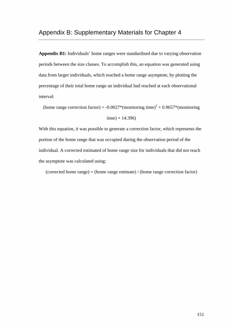
151
Appendix B: Supplementary Materials for Chapter 4
Appendix B1: Individuals’ home ranges were standardised due to varying observation
periods between the size classes. To accomplish this, an equation was generated using
data from larger individuals, which reached a home range asymptote, by plotting the
percentage of their total home range an individual had reached at each observational
interval:
(home range correction factor) = -0.0027*(monitoring time)2 + 0.9657*(monitoring
time) + 14.396)
With this equation, it was possible to generate a correction factor, which represents the
portion of the home range that was occupied during the observation period of the
individual. A corrected estimated of home range size for individuals that did not reach
the asymptote was calculated using:
(corrected home range) = (home range estimate) / (home range correction factor)
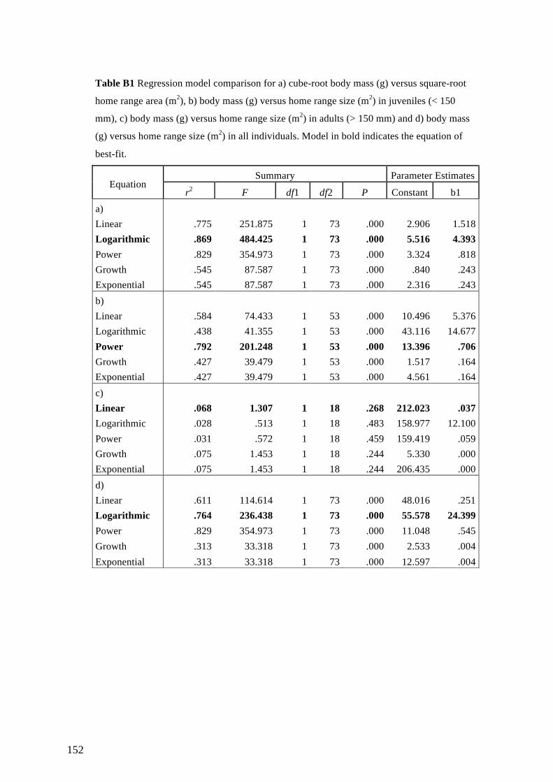
152
Table B1 Regression model comparison for a) cube-root body mass (g) versus square-root
home range area (m2), b) body mass (g) versus home range size (m2) in juveniles (< 150
mm), c) body mass (g) versus home range size (m2) in adults (> 150 mm) and d) body mass
(g) versus home range size (m2) in all individuals. Model in bold indicates the equation of
best-fit.
Equation Summary Parameter Estimates
r2 F df1 df2 P Constant b1 a) Linear .775 251.875 1 73 .000 2.906 1.518 Logarithmic .869 484.425 1 73 .000 5.516 4.393 Power .829 354.973 1 73 .000 3.324 .818 Growth .545 87.587 1 73 .000 .840 .243 Exponential .545 87.587 1 73 .000 2.316 .243 b) Linear .584 74.433 1 53 .000 10.496 5.376 Logarithmic .438 41.355 1 53 .000 43.116 14.677 Power .792 201.248 1 53 .000 13.396 .706 Growth .427 39.479 1 53 .000 1.517 .164 Exponential .427 39.479 1 53 .000 4.561 .164 c) Linear .068 1.307 1 18 .268 212.023 .037 Logarithmic .028 .513 1 18 .483 158.977 12.100 Power .031 .572 1 18 .459 159.419 .059 Growth .075 1.453 1 18 .244 5.330 .000 Exponential .075 1.453 1 18 .244 206.435 .000 d) Linear .611 114.614 1 73 .000 48.016 .251 Logarithmic .764 236.438 1 73 .000 55.578 24.399 Power .829 354.973 1 73 .000 11.048 .545 Growth .313 33.318 1 73 .000 2.533 .004 Exponential .313 33.318 1 73 .000 12.597 .004
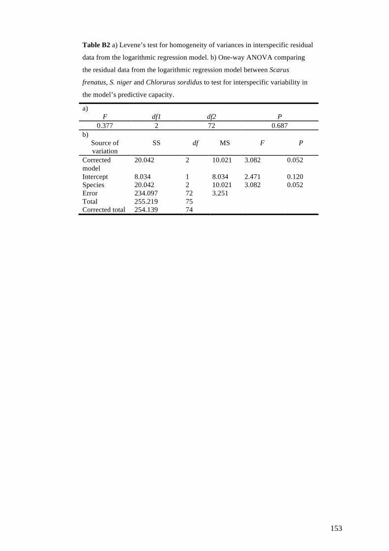
153
Table B2 a) Levene’s test for homogeneity of variances in interspecific residual
data from the logarithmic regression model. b) One-way ANOVA comparing
the residual data from the logarithmic regression model between Scarus
frenatus, S. niger and Chlorurus sordidus to test for interspecific variability in
the model’s predictive capacity.
a) F df1 df2 P
0.377 2 72 0.687 b)
Source of variation
SS df MS F P
Corrected model
20.042 2 10.021 3.082 0.052
Intercept 8.034 1 8.034 2.471 0.120 Species 20.042 2 10.021 3.082 0.052 Error 234.097 72 3.251 Total 255.219 75 Corrected total 254.139 74
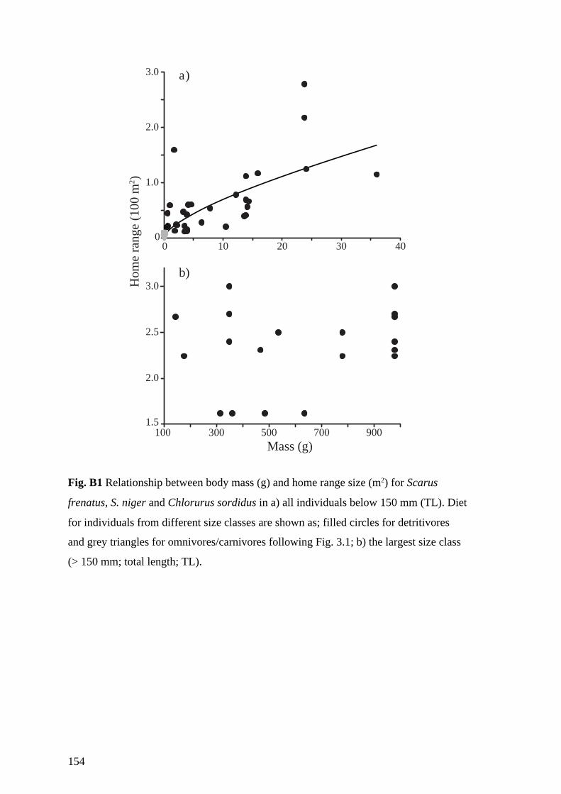
154
Fig. B1 Relationship between body mass (g) and home range size (m2) for Scarus
frenatus, S. niger and Chlorurus sordidus in a) all individuals below 150 mm (TL). Diet
for individuals from different size classes are shown as; filled circles for detritivores
and grey triangles for omnivores/carnivores following Fig. 3.1; b) the largest size class
(> 150 mm; total length; TL).
Mass (g)
0 10 20 30 40
Hom
e ra
nge
(100
m2 )
0
1.0
2.0
3.0 a)
100 300 500 700 900
b)
1.5
2.0
2.5
3.0
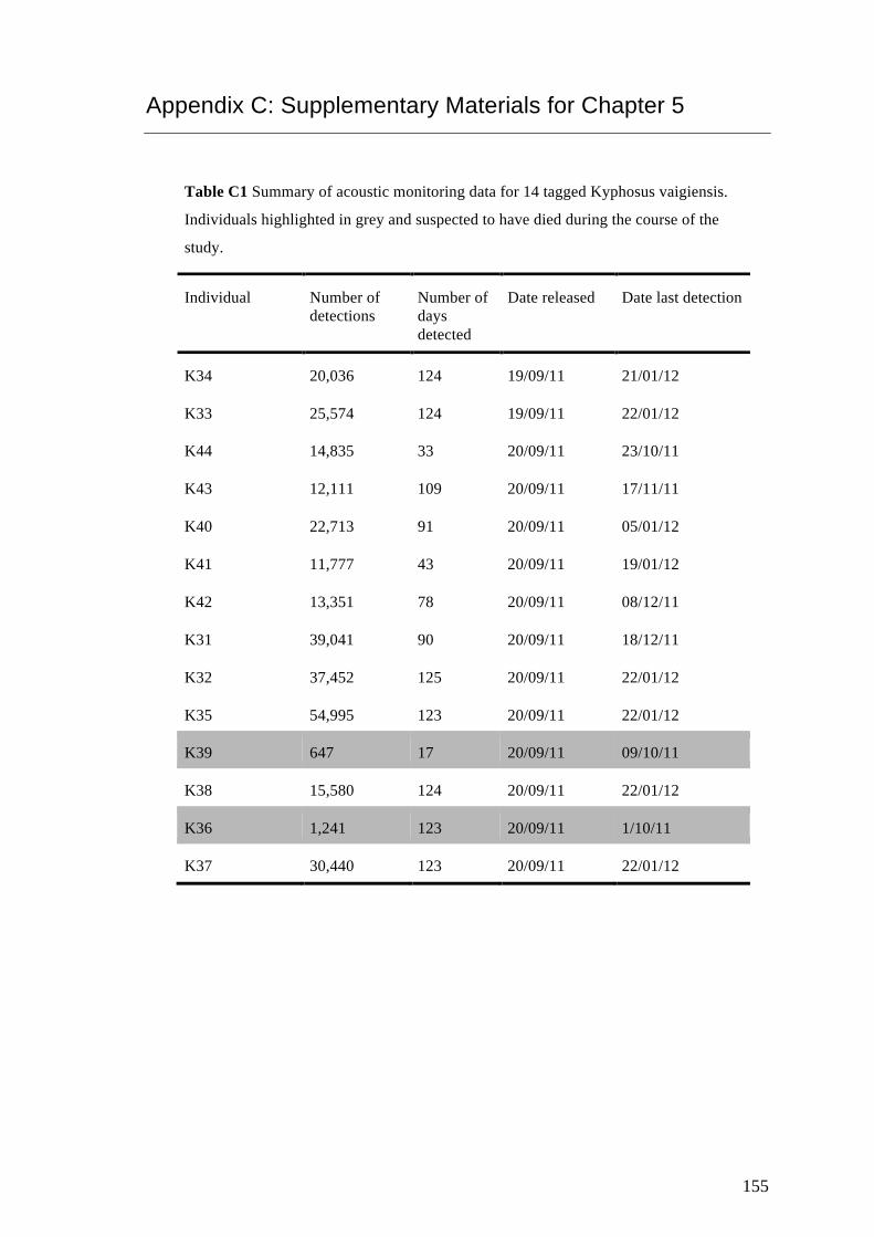
155
Appendix C: Supplementary Materials for Chapter 5
Table C1 Summary of acoustic monitoring data for 14 tagged Kyphosus vaigiensis.
Individuals highlighted in grey and suspected to have died during the course of the
study.
Individual Number of detections
Number of days detected
Date released Date last detection
K34 20,036 124 19/09/11 21/01/12
K33 25,574 124 19/09/11 22/01/12
K44 14,835 33 20/09/11 23/10/11
K43 12,111 109 20/09/11 17/11/11
K40 22,713 91 20/09/11 05/01/12
K41 11,777 43 20/09/11 19/01/12
K42 13,351 78 20/09/11 08/12/11
K31 39,041 90 20/09/11 18/12/11
K32 37,452 125 20/09/11 22/01/12
K35 54,995 123 20/09/11 22/01/12
K39 647 17 20/09/11 09/10/11
K38 15,580 124 20/09/11 22/01/12
K36 1,241 123 20/09/11 1/10/11
K37 30,440 123 20/09/11 22/01/12
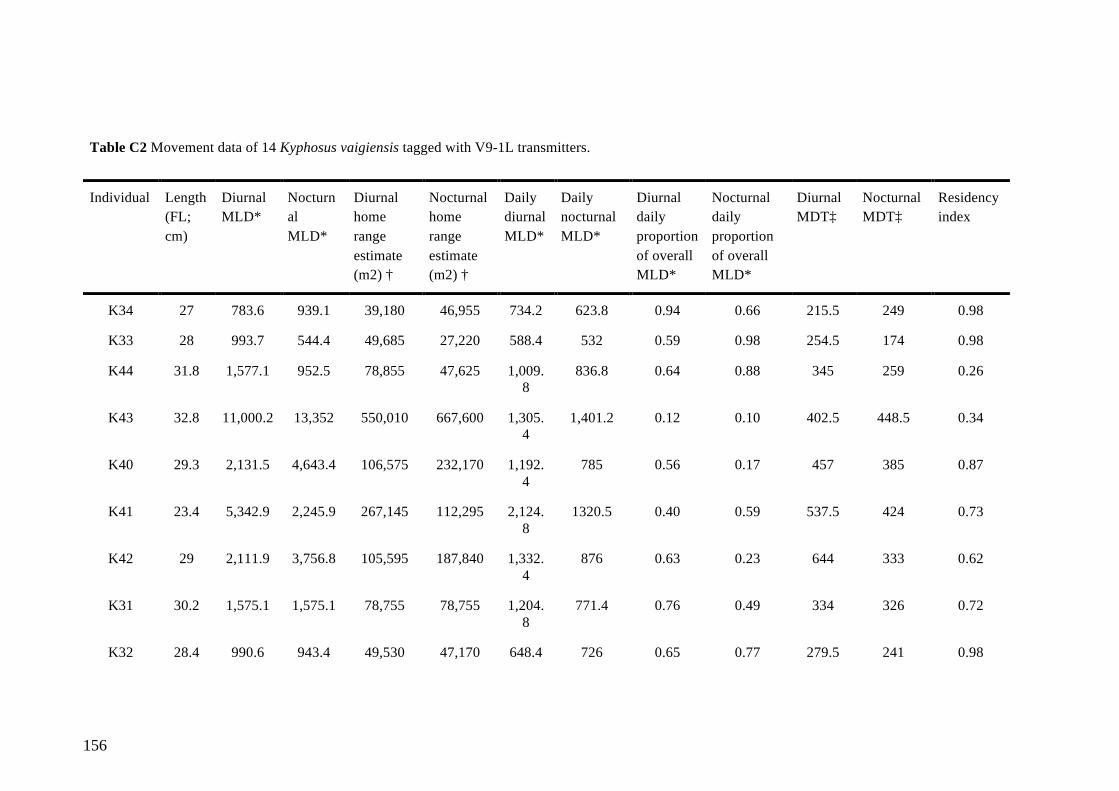
156
Table C2 Movement data of 14 Kyphosus vaigiensis tagged with V9-1L transmitters.
Individual Length (FL; cm)
Diurnal MLD*
Nocturnal MLD*
Diurnal home range estimate (m2) †
Nocturnal home range estimate (m2) †
Daily diurnal MLD*
Daily nocturnal MLD*
Diurnal daily proportion of overall MLD*
Nocturnal daily proportion of overall MLD*
Diurnal MDT‡
Nocturnal MDT‡
Residency index
K34 27 783.6 939.1 39,180 46,955 734.2 623.8 0.94 0.66 215.5 249 0.98
K33 28 993.7 544.4 49,685 27,220 588.4 532 0.59 0.98 254.5 174 0.98
K44 31.8 1,577.1 952.5 78,855 47,625 1,009.8
836.8 0.64 0.88 345 259 0.26
K43 32.8 11,000.2 13,352 550,010 667,600 1,305.4
1,401.2 0.12 0.10 402.5 448.5 0.34
K40 29.3 2,131.5 4,643.4 106,575 232,170 1,192.4
785 0.56 0.17 457 385 0.87
K41 23.4 5,342.9 2,245.9 267,145 112,295 2,124.8
1320.5 0.40 0.59 537.5 424 0.73
K42 29 2,111.9 3,756.8 105,595 187,840 1,332.4
876 0.63 0.23 644 333 0.62
K31 30.2 1,575.1 1,575.1 78,755 78,755 1,204.8
771.4 0.76 0.49 334 326 0.72
K32 28.4 990.6 943.4 49,530 47,170 648.4 726 0.65 0.77 279.5 241 0.98
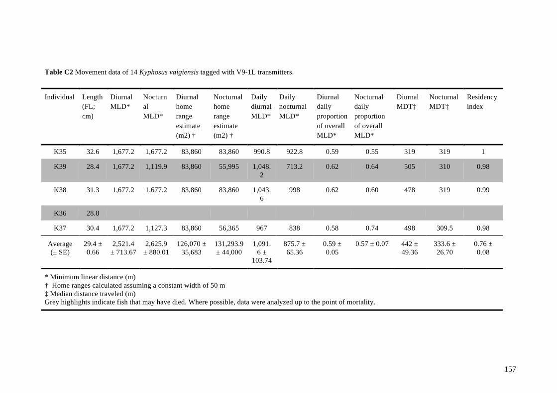
157
Table C2 Movement data of 14 Kyphosus vaigiensis tagged with V9-1L transmitters.
Individual Length (FL; cm)
Diurnal MLD*
Nocturnal MLD*
Diurnal home range estimate (m2) †
Nocturnal home range estimate (m2) †
Daily diurnal MLD*
Daily nocturnal MLD*
Diurnal daily proportion of overall MLD*
Nocturnal daily proportion of overall MLD*
Diurnal MDT‡
Nocturnal MDT‡
Residency index
K35 32.6 1,677.2 1,677.2 83,860 83,860 990.8 922.8 0.59 0.55 319 319 1
K39 28.4 1,677.2 1,119.9 83,860 55,995 1,048.2
713.2 0.62 0.64 505 310 0.98
K38 31.3 1,677.2 1,677.2 83,860 83,860 1,043.6
998 0.62 0.60 478 319 0.99
K36 28.8
K37 30.4 1,677.2 1,127.3 83,860 56,365 967 838 0.58 0.74 498 309.5 0.98
Average (± SE)
29.4 ± 0.66
2,521.4 ± 713.67
2,625.9 ± 880.01
126,070 ± 35,683
131,293.9 ± 44,000
1,091.6 ±
103.74
875.7 ± 65.36
0.59 ± 0.05
0.57 ± 0.07 442 ± 49.36
333.6 ± 26.70
0.76 ± 0.08
* Minimum linear distance (m) † Home ranges calculated assuming a constant width of 50 m ‡ Median distance traveled (m) Grey highlights indicate fish that may have died. Where possible, data were analyzed up to the point of mortality.
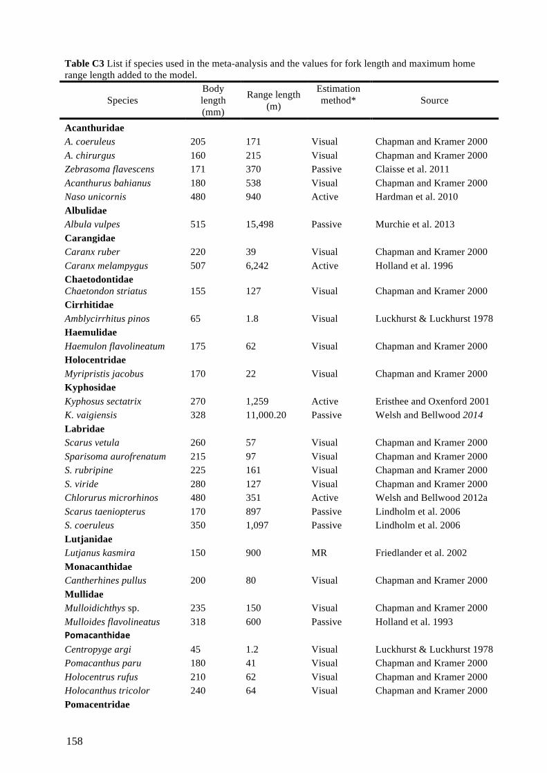
158
Table C3 List if species used in the meta-analysis and the values for fork length and maximum home range length added to the model.
Species Body length (mm)
Range length (m)
Estimation method*
Source
Acanthuridae A. coeruleus 205 171 Visual Chapman and Kramer 2000
A. chirurgus 160 215 Visual Chapman and Kramer 2000 Zebrasoma flavescens 171 370 Passive Claisse et al. 2011 Acanthurus bahianus 180 538 Visual Chapman and Kramer 2000 Naso unicornis 480 940 Active Hardman et al. 2010 Albulidae
Albula vulpes 515 15,498 Passive Murchie et al. 2013 Carangidae
Caranx ruber 220 39 Visual Chapman and Kramer 2000 Caranx melampygus 507 6,242 Active Holland et al. 1996 Chaetodontidae
Chaetondon striatus 155 127 Visual Chapman and Kramer 2000 Cirrhitidae
Amblycirrhitus pinos 65 1.8 Visual Luckhurst & Luckhurst 1978 Haemulidae
Haemulon flavolineatum 175 62 Visual Chapman and Kramer 2000 Holocentridae
Myripristis jacobus 170 22 Visual Chapman and Kramer 2000 Kyphosidae
Kyphosus sectatrix 270 1,259 Active Eristhee and Oxenford 2001 K. vaigiensis 328 11,000.20 Passive Welsh and Bellwood 2014 Labridae
Scarus vetula 260 57 Visual Chapman and Kramer 2000 Sparisoma aurofrenatum 215 97 Visual Chapman and Kramer 2000 S. rubripine 225 161 Visual Chapman and Kramer 2000 S. viride 280 127 Visual Chapman and Kramer 2000 Chlorurus microrhinos 480 351 Active Welsh and Bellwood 2012a Scarus taeniopterus 170 897 Passive Lindholm et al. 2006 S. coeruleus 350 1,097 Passive Lindholm et al. 2006 Lutjanidae
Lutjanus kasmira 150 900 MR Friedlander et al. 2002 Monacanthidae
Cantherhines pullus 200 80 Visual Chapman and Kramer 2000 Mullidae
Mulloidichthys sp. 235 150 Visual Chapman and Kramer 2000 Mulloides flavolineatus 318 600 Passive Holland et al. 1993 Pomacanthidae,
Centropyge argi 45 1.2 Visual Luckhurst & Luckhurst 1978 Pomacanthus paru 180 41 Visual Chapman and Kramer 2000 Holocentrus rufus 210 62 Visual Chapman and Kramer 2000 Holocanthus tricolor 240 64 Visual Chapman and Kramer 2000 Pomacentridae
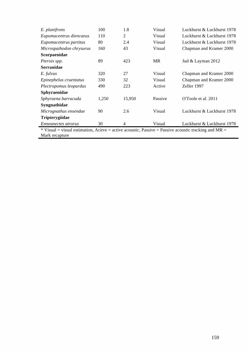
159
E. planifrons 100 1.8 Visual Luckhurst & Luckhurst 1978 Eupomacentrus diencaeus 110 2 Visual Luckhurst & Luckhurst 1978 Eupomacentrus partitus 80 2.4 Visual Luckhurst & Luckhurst 1978 Microspathodon chrysurus 160 43 Visual Chapman and Kramer 2000 Scorpaenidae
Pterois spp. 89 423 MR Jud & Layman 2012 Serranidae
E. fulvus 320 27 Visual Chapman and Kramer 2000 Epinephelus cruentatus 330 32 Visual Chapman and Kramer 2000 Plectropomus leopardus 490 223 Active Zeller 1997 Sphyraenidae
Sphyraena barracuda 1,250 15,950 Passive O'Toole et al. 2011 Syngnathidae
Micrognathus ensendae 90 2.6 Visual Luckhurst & Luckhurst 1978 Tripterygiidae
Enneanectes atrorus 30 4 Visual Luckhurst & Luckhurst 1978 * Visual = visual estimation, Acitve = active acoustic, Passive = Passive acoustic tracking and MR = Mark recapture
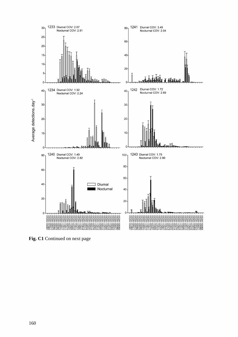
160
Fig. C1 Continued on next page

161
Fig. C1 Continued on next page
1244
1231
1232
1237
1235
1238
VR
2W-109081
VR
2W-101865
VR
2W-109071
VR
2W-109073
VR
2W-109082
VR
2W-109074
VR
2W-109066
VR
2W-109072
VR
2W-112617
VR
2W-112610
VR
2W-112611
VR
2W-105219
VR
2W-105221
VR
2W-112624
VR
2W-105222
VR
2W-112618
VR
2W-105217
VR
2W-112622
VR
2W-112621
VR
2W-112616
VR
2W-105215
VR
2W-109079
VR
2W-112612
VR
2W-105220
VR
2W-105214
VR
2W-105216
VR
2W-112623
VR
2W-112614
VR
2W-112613
VR
2W-109026
VR
2W-105213
VR
2W-112615
VR
2W-112620
VR
2W-105218
VR
2W-112619
VR
2W-109069
VR
2W-109070
VR
2W-109077
VR
2W-109080
VR
2W-109068
VR
2W-109081
VR
2W-101865
VR
2W-109071
VR
2W-109073
VR
2W-109082
VR
2W-109074
VR
2W-109066
VR
2W-109072
VR
2W-112617
VR
2W-112610
VR
2W-112611
VR
2W-105219
VR
2W-105221
VR
2W-112624
VR
2W-105222
VR
2W-112618
VR
2W-105217
VR
2W-112622
VR
2W-112621
VR
2W-112616
VR
2W-105215
VR
2W-109079
VR
2W-112612
VR
2W-105220
VR
2W-105214
VR
2W-105216
VR
2W-112623
VR
2W-112614
VR
2W-112613
VR
2W-109026
VR
2W-105213
VR
2W-112615
VR
2W-112620
VR
2W-105218
VR
2W-112619
VR
2W-109069
VR
2W-109070
VR
2W-109077
VR
2W-109080
VR
2W-109068
120
100
80
60
40
20
0
60
50
40
30
20
10
0
60
50
40
30
20
10
0
100
80
60
40
20
0
30
25
20
15
10
5
0
20
18
16
14
12
10
8
6
4
2
0
Ave
rage
det
ectio
ns.d
ay-1
Diurnal Nocturnal
Diurnal COV: 1.31Nocturnal COV: 2.88
Diurnal COV: 1.09Nocturnal COV: 2.20
Diurnal COV: 0.84Nocturnal COV: 1.82
Diurnal COV: 1.21Nocturnal COV: 1.57
Diurnal COV: 1.58Nocturnal COV: 2.77
Diurnal COV: 1.55Nocturnal COV: 1.55

162
Fig. C1 Average number of detections per day for each tagged Kyphosus vaigiensis (±
SE) plotted across the acoustic array (plotted from the Northern to the South point of
Orpheus Island). Diurnal and nocturnal detections are plotted separately.
1239
VR
2W-109081
VR
2W-101865
VR
2W-109071
VR
2W-109073
VR
2W-109082
VR
2W-109074
VR
2W-109066
VR
2W-109072
VR
2W-112617
VR
2W-112610
VR
2W-112611
VR
2W-105219
VR
2W-105221
VR
2W-112624
VR
2W-105222
VR
2W-112618
VR
2W-105217
VR
2W-112622
VR
2W-112621
VR
2W-112616
VR
2W-105215
VR
2W-109079
VR
2W-112612
VR
2W-105220
VR
2W-105214
VR
2W-105216
VR
2W-112623
VR
2W-112614
VR
2W-112613
VR
2W-109026
VR
2W-105213
VR
2W-112615
VR
2W-112620
VR
2W-105218
VR
2W-112619
VR
2W-109069
VR
2W-109070
VR
2W-109077
VR
2W-109080
VR
2W-109068
30
25
20
15
10
5
0
Ave
rage
det
ectio
ns.d
ay-1
Diurnal Nocturnal
Diurnal COV: 1.21Nocturnal COV: 1.57
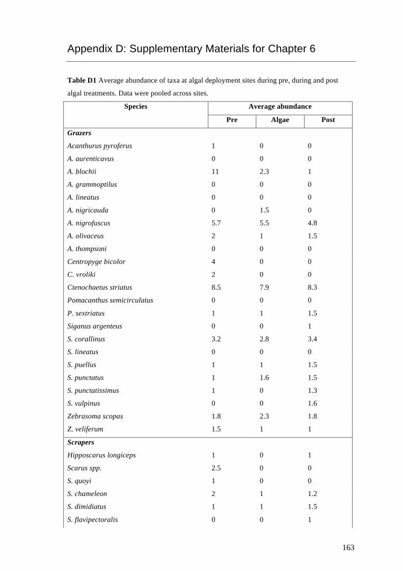
163
Appendix D: Supplementary Materials for Chapter 6
Table D1 Average abundance of taxa at algal deployment sites during pre, during and post
algal treatments. Data were pooled across sites.
Species Average abundance
Pre Algae Post
Grazers
Acanthurus pyroferus 1 0 0
A. aurenticavus 0 0 0
A. blochii 11 2.3 1
A. grammoptilus 0 0 0
A. lineatus 0 0 0
A. nigricauda 0 1.5 0
A. nigrofuscus 5.7 5.5 4.8
A. olivaceus 2 1 1.5
A. thompsoni 0 0 0
Centropyge bicolor 4 0 0
C. vroliki 2 0 0
Ctenochaetus striatus 8.5 7.9 8.3
Pomacanthus semicirculatus 0 0 0
P. sextriatus 1 1 1.5
Siganus argenteus 0 0 1
S. corallinus 3.2 2.8 3.4
S. lineatus 0 0 0
S. puellus 1 1 1.5
S. punctatus 1 1.6 1.5
S. punctatissimus 1 0 1.3
S. vulpinus 0 0 1.6
Zebrasoma scopas 1.8 2.3 1.8
Z. veliferum 1.5 1 1
Scrapers
Hipposcarus longiceps 1 0 1
Scarus spp. 2.5 0 0
S. quoyi 1 0 0
S. chameleon 2 1 1.2
S. dimidiatus 1 1 1.5
S. flavipectoralis 0 0 1
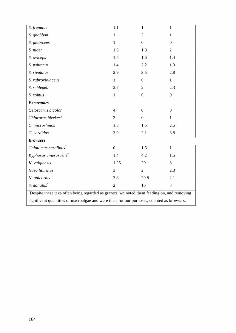
164
S. frenatus 1.1 1 1
S. ghobban 1 2 1
S. globiceps 1 0 0
S. niger 1.6 1.8 2
S. oviceps 1.5 1.6 1.4
S. psittacus 1.4 2.2 1.3
S. rivulatus 2.9 3.5 2.8
S. rubroviolaceus 1 0 1
S. schlegeli 2.7 2 2.3
S. spinus 1 0 0
Excavators
Cetoscarus bicolor 4 0 0
Chlorurus bleekeri 3 0 1
C. microrhinos 1.3 1.5 2.5
C. sordidus 3.9 2.1 3.8
Browsers
Calotomus carolinus* 0 1.6 1
Kyphosus cinerascens* 1.4 4.2 1.5
K. vaigiensis 1.25 20 3
Naso lituratus 3 2 2.3
N. unicornis 3.8 29.8 2.1
S. doliatus* 2 16 3 *Despite these taxa often being regarded as grazers, we noted them feeding on, and removing
significant quantities of macroalgae and were thus, for our purposes, counted as browsers.
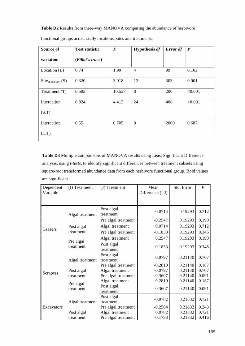
165
Table D2 Results from three-way MANOVA comparing the abundance of herbivore
functional groups across study locations, sites and treatments.
Source of
variation
Test statistic
(Pillai’s trace)
F Hypothesis df Error df P
Location (L) 0.74 1.99 4 99 0.102
Site(Location) (S) 0.320 3.018 12 303 0.001
Treatment (T) 0.593 10.537 8 200 <0.001
Interaction
(S.T)
0.824 4.412 24 408 <0.001
Interaction
(L.T)
0.55 0.705 8 2000 0.687
Table D3 Multiple comparisons of MANOVA results using Least Significant Difference
analysis, using t-tests, to identify significant differences between treatment subsets using
square-root transformed abundance data from each herbivore functional group. Bold values
are significant.
Dependent Variable
(I) Treatment (J) Treatment Mean Difference (I-J)
Std. Error P
Grazers
Algal treatment Post algal treatment -0.0714 0.19293 0.712
Pre algal treatment -0.2547 0.19293 0.190 Post algal treatment
Algal treatment 0.0714 0.19293 0.712 Pre algal treatment -0.1833 0.19293 0.345
Pre algal treatment
Algal treatment 0.2547 0.19293 0.190 Post algal treatment 0.1833 0.19293 0.345
Scrapers
Algal treatment Post algal treatment 0.0797 0.21140 0.707
Pre algal treatment -0.2810 0.21140 0.187 Post algal treatment
Algal treatment -0.0797 0.21140 0.707 Pre algal treatment -0.3607 0.21140 0.091
Pre algal treatment
Algal treatment 0.2810 0.21140 0.187 Post algal treatment 0.3607 0.21140 0.091
Excavators Algal treatment
Post algal treatment -0.0782 0.21832 0.721
Pre algal treatment -0.2564 0.21832 0.243 Post algal treatment
Algal treatment 0.0782 0.21832 0.721 Pre algal treatment -0.1783 0.21832 0.416
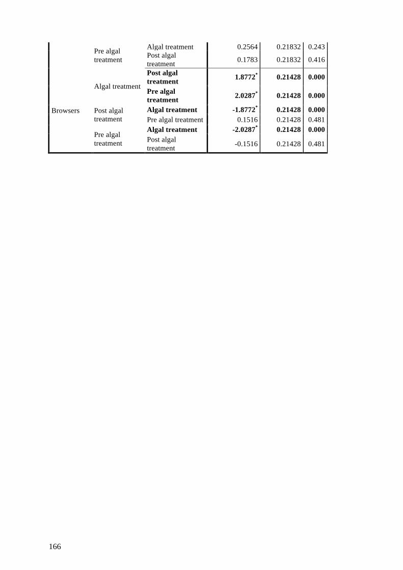
166
Pre algal treatment
Algal treatment 0.2564 0.21832 0.243 Post algal treatment 0.1783 0.21832 0.416
Browsers
Algal treatment
Post algal treatment 1.8772* 0.21428 0.000
Pre algal treatment 2.0287* 0.21428 0.000
Post algal treatment
Algal treatment -1.8772* 0.21428 0.000 Pre algal treatment 0.1516 0.21428 0.481
Pre algal treatment
Algal treatment -2.0287* 0.21428 0.000 Post algal treatment -0.1516 0.21428 0.481
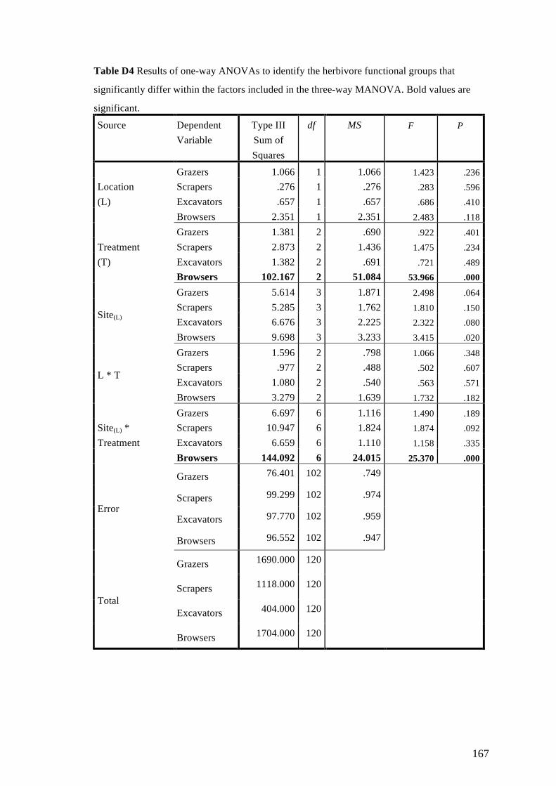
167
Table D4 Results of one-way ANOVAs to identify the herbivore functional groups that
significantly differ within the factors included in the three-way MANOVA. Bold values are
significant.
Source Dependent Variable
Type III Sum of Squares
df MS F P
Location (L)
Grazers 1.066 1 1.066 1.423 .236 Scrapers .276 1 .276 .283 .596 Excavators .657 1 .657 .686 .410 Browsers 2.351 1 2.351 2.483 .118
Treatment (T)
Grazers 1.381 2 .690 .922 .401 Scrapers 2.873 2 1.436 1.475 .234 Excavators 1.382 2 .691 .721 .489 Browsers 102.167 2 51.084 53.966 .000
Site(L)
Grazers 5.614 3 1.871 2.498 .064 Scrapers 5.285 3 1.762 1.810 .150 Excavators 6.676 3 2.225 2.322 .080 Browsers 9.698 3 3.233 3.415 .020
L * T
Grazers 1.596 2 .798 1.066 .348 Scrapers .977 2 .488 .502 .607 Excavators 1.080 2 .540 .563 .571 Browsers 3.279 2 1.639 1.732 .182
Site(L) * Treatment
Grazers 6.697 6 1.116 1.490 .189 Scrapers 10.947 6 1.824 1.874 .092 Excavators 6.659 6 1.110 1.158 .335 Browsers 144.092 6 24.015 25.370 .000
Error
Grazers 76.401 102 .749
Scrapers 99.299 102 .974
Excavators 97.770 102 .959
Browsers 96.552 102 .947
Total
Grazers 1690.000 120
Scrapers 1118.000 120
Excavators 404.000 120
Browsers 1704.000 120

168
Table D5 Number of each herbivorous taxa captured and successfully monitored and their
estimated abundance at each study site.
Species Site Number tagged
(average size; range
[cm])
Mean abundance ±
SE (max) based on
data from visual
census
S. vulpinus Mermaid 4 (22; 21.5 – 22.5) 1 ± 1.0 (4)
S. vulpinus Turtle 2 (22.8; 22.5 – 23) 0.25 ± 0.25 (2)
S. corallinus Mermaid 4 (20.3; 18.5 – 22) 5 ± 2.6 (10)
S. corallinus Turtle 2 (22.3; 22 – 22.5) 3.75 ± 2.5 (4)
Sc. schlegeli Mermaid 8 (24.4; 17.5 – 29.5) 8.8 ± 1.8 (13)
Sc. schlegeli Turtle 9 (25.9; 19.5 –31) 15 ± 1.7 (20)
N. unicornis Mermaid 2 (24.8; 20 – 28) 3 ± 0.9 (5)
N. unicornis Turtle 1 (22.9; no range) 1.5 ± 0.3 (2)
Table D6 Average fish abundance in Mermaid Cove and Turtle Bay
derived from underwater visual transects.
Average fish abundance per 40 m2
± SE
Species Mermaid Turtle
Acanthurus blochii 1 ± 1 1 ± 1
A. lineatus 19.25 ± 4.71 5 ± 2.68
A. nigrocauda 2 ± 0.91 0.25 ± 0.25
A. nigrofuscus 17 ± 8.37 0.25 ± 0.25
A. olivaceus 1 ± 0.58 1.25 ± 0.48
A. pyroferus 0.25 ± 0.25 18.25 ± 5.12
Calotomus carolinus 0.25 ± 0.25 3.75 ± 1.89
Cetoscarus bicolor 1.25 ± 0.63 1 ± 0.41
Chlorurus bleekeri 0.25 ± 0.25 1.5 ± 0.29
C. microrhinos 1 ± 0 9.75 ± 3.40
C. sordidus 10.5 ± 2.22 24.25 ± 3.09
Ctenochaetus binotatus 0.25 ± 0.25 0.25 ± 0.25
C. striatus 61.75 ± 8.21 3 ± 1.08
Kyphosus vaigiensis 5.75 ± 2.02 4.5 ± 1.32
Naso brachycentron 0.25 ± 0.25 4 ± 4
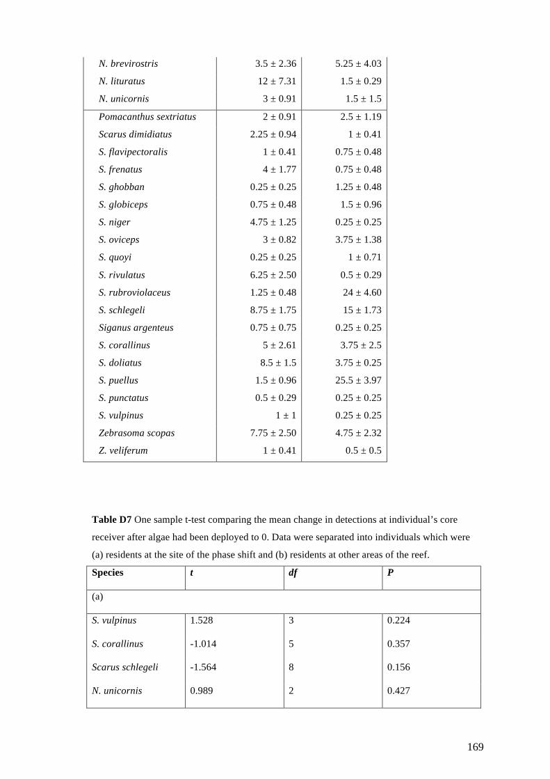
169
N. brevirostris 3.5 ± 2.36 5.25 ± 4.03
N. lituratus 12 ± 7.31 1.5 ± 0.29
N. unicornis 3 ± 0.91 1.5 ± 1.5
Pomacanthus sextriatus 2 ± 0.91 2.5 ± 1.19
Scarus dimidiatus 2.25 ± 0.94 1 ± 0.41
S. flavipectoralis 1 ± 0.41 0.75 ± 0.48
S. frenatus 4 ± 1.77 0.75 ± 0.48
S. ghobban 0.25 ± 0.25 1.25 ± 0.48
S. globiceps 0.75 ± 0.48 1.5 ± 0.96
S. niger 4.75 ± 1.25 0.25 ± 0.25
S. oviceps 3 ± 0.82 3.75 ± 1.38
S. quoyi 0.25 ± 0.25 1 ± 0.71
S. rivulatus 6.25 ± 2.50 0.5 ± 0.29
S. rubroviolaceus 1.25 ± 0.48 24 ± 4.60
S. schlegeli 8.75 ± 1.75 15 ± 1.73
Siganus argenteus 0.75 ± 0.75 0.25 ± 0.25
S. corallinus 5 ± 2.61 3.75 ± 2.5
S. doliatus 8.5 ± 1.5 3.75 ± 0.25
S. puellus 1.5 ± 0.96 25.5 ± 3.97
S. punctatus 0.5 ± 0.29 0.25 ± 0.25
S. vulpinus 1 ± 1 0.25 ± 0.25
Zebrasoma scopas 7.75 ± 2.50 4.75 ± 2.32
Z. veliferum 1 ± 0.41 0.5 ± 0.5
Table D7 One sample t-test comparing the mean change in detections at individual’s core
receiver after algae had been deployed to 0. Data were separated into individuals which were
(a) residents at the site of the phase shift and (b) residents at other areas of the reef.
Species t df P
(a)
S. vulpinus 1.528 3 0.224
S. corallinus -1.014 5 0.357
Scarus schlegeli -1.564 8 0.156
N. unicornis 0.989 2 0.427
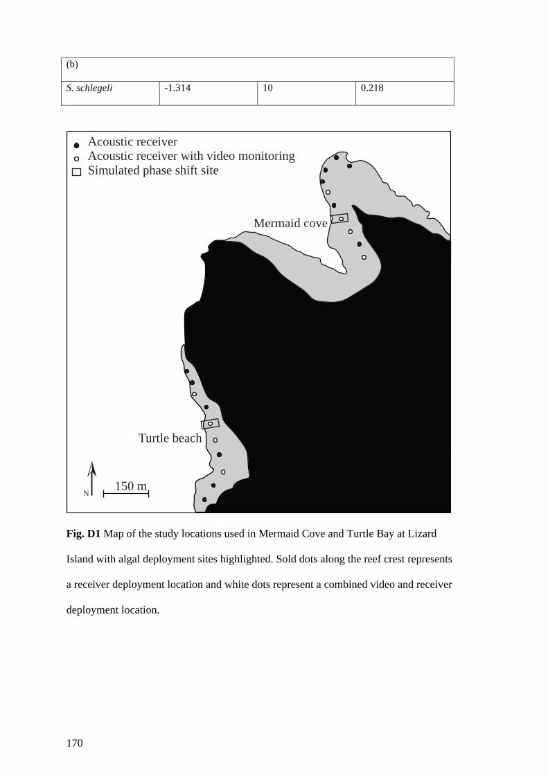
170
(b)
S. schlegeli -1.314 10 0.218
Fig. D1 Map of the study locations used in Mermaid Cove and Turtle Bay at Lizard
Island with algal deployment sites highlighted. Sold dots along the reef crest represents
a receiver deployment location and white dots represent a combined video and receiver
deployment location.
150 m
Acoustic receiver with video monitoringSimulated phase shift site
N
Acoustic receiver
Mermaid cove
Turtle beach
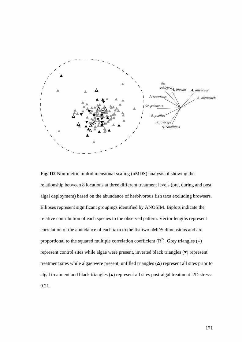
171
Fig. D2 Non-metric multidimensional scaling (nMDS) analysis of showing the
relationship between 8 locations at three different treatment levels (pre, during and post
algal deployment) based on the abundance of herbivorous fish taxa excluding browsers.
Ellipses represent significant groupings identified by ANOSIM. Biplots indicate the
relative contribution of each species to the observed pattern. Vector lengths represent
correlation of the abundance of each taxa to the fist two nMDS dimensions and are
proportional to the squared multiple correlation coefficient (R2). Grey triangles ( )
represent control sites while algae were present, inverted black triangles ( ) represent
treatment sites while algae were present, unfilled triangles ( ) represent all sites prior to
algal treatment and black triangles ( ) represent all sites post-algal treatment. 2D stress:
0.21.
A. blochii
A. nigricauda
A. olivaceus
P. sextriatus
Sc. oviceps
Sc. psittacus
Sc. schlegeli
S. corallinus
S. puellus
172
Appendix E: Assessment of the impact of acoustic tagging
on fish mortality and behaviour Several studies have quantified the effects of tagging fish with acoustic transmitters,
with the goal of estimating behavioural modifications or enhanced mortality as a result
of the tagging process (Zeller 1999; Lower et al. 2005; Bellquist et al. 2008). These
works have overwhelmingly found that the internal tagging of fishes has little to no
effect on fish, with few exceptions. This is especially true for more recent studies that
employ refined surgical techniques and use smaller transmitters (Hutchinson and
Rhodes 2010; Marshell et al. 2011; Welsh and Bellwood 2012a, b). Indeed, the studies
enclosed in the present thesis corroborate this finding. Of the fish tagged herein, very
few were recorded to have died immediately following transmitter implantation (Table
E1). This suggests that the acute effects of internal tagging on the survival of reef fishes
appear to be minimal. However, behavioural modifications as a result of tagging have
been suggested to undermine the results of studies that utilize acoustic tagging.
The combination of movement data into ecological studies is among the novel
aspects of the present studies, and also affords us the ability to directly assess the
changes in a fish’s behavior following tagging. By monitoring a fish’s activity
following tagging, in conjunction with conspecifics, it is possible to identify underlying
subtle behavioural changes that may arise as a result of tagging. This is reported in
Welsh and Bellwood (2012a) in which the home range of Chlorurus microrhinos was
monitored using intensive active acoustic tracking. The study also monitored the
movements and behaviours of the tagged individual’s social groups to identify any
irregularities from the tagged specimen. Despite being tagged with an internal
transmitter, within hours of being released onto the reef, tagged fishes exhibited no
irregular behavior and moved with other harem members. Furthermore, these

173
individuals exhibited no change in social status or sex during the period of the study. In
the present studies, the behaviour of another parrotfish Scarus rivulatus was assessed in
a similar manner. Both tagged and non-tagged individuals were simultaneously
monitored for several weeks after tagging with their feeding behaviours, schooling
proclivities and social status recorded. Despite the intensive monitoring of tagged
individuals, no irregularities were detected and the movements and feeding of tagged
fishes remained indistinguishable from their conspecifics.
Unusual bahviours have however been reported following tagging however, the
explanation for these irregularities may not be directly attributed to the implanted
transmitter. Chateau and Wantiez (2009) report an individual Chlorurus microrhinos
moving 6 km, between reefs, following release. This finding is in direct contrast to the
findings of Welsh and Bellwood (2012a) for the same species, which only report highly
site-attached behaviours with restricted movements. This distinction is likely to arise as
a result of the tagging procedures used in the two studies. In the former study,
individuals are held in captivity for long periods of time (4.3 + 2.7 days) while the latter
kept individuals captive for a maximum of 24 h. Such excessive recovery periods in
captivity may have cause the C. microrhinos to be displaced from their social group or
territory resulting in a shift from site-attached, normal movements, to dispersive
movements as they search for a new territory or social group to join (Ogden and
Buckman 1973; van Rooij et al. 1996). Thus, while captive holding times of several
days are not unusual in the literature (e.g. Marshell et al. 2011), and have been highly
recommended by some works (Zeller 1999), it is important to consider the behavioural
implications of such removal times, and how these practices may fundamentally alter
the ‘normal’ movements of some taxa.
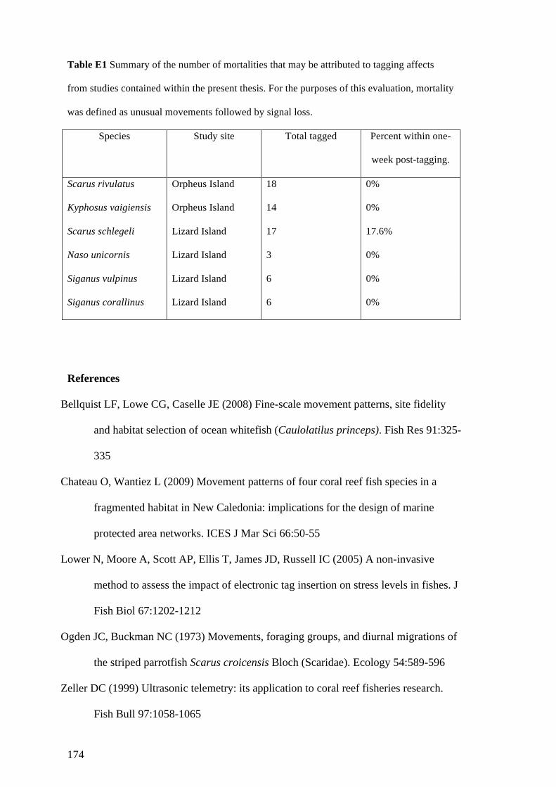
174
Table E1 Summary of the number of mortalities that may be attributed to tagging affects
from studies contained within the present thesis. For the purposes of this evaluation, mortality
was defined as unusual movements followed by signal loss.
Species Study site Total tagged Percent within one-
week post-tagging.
Scarus rivulatus Orpheus Island 18 0%
Kyphosus vaigiensis Orpheus Island 14 0%
Scarus schlegeli Lizard Island 17 17.6%
Naso unicornis Lizard Island 3 0%
Siganus vulpinus Lizard Island 6 0%
Siganus corallinus Lizard Island 6 0%
References
Bellquist LF, Lowe CG, Caselle JE (2008) Fine-scale movement patterns, site fidelity
and habitat selection of ocean whitefish (Caulolatilus princeps). Fish Res 91:325-
335
Chateau O, Wantiez L (2009) Movement patterns of four coral reef fish species in a
fragmented habitat in New Caledonia: implications for the design of marine
protected area networks. ICES J Mar Sci 66:50-55
Lower N, Moore A, Scott AP, Ellis T, James JD, Russell IC (2005) A non-invasive
method to assess the impact of electronic tag insertion on stress levels in fishes. J
Fish Biol 67:1202-1212
Ogden JC, Buckman NC (1973) Movements, foraging groups, and diurnal migrations of
the striped parrotfish Scarus croicensis Bloch (Scaridae). Ecology 54:589-596
Zeller DC (1999) Ultrasonic telemetry: its application to coral reef fisheries research.
Fish Bull 97:1058-1065
175
Appendix F: Publications arising from thesis
Publications derived from thesis chapters
Welsh JQ, Fox RJ, Webber DM, Bellwood DR (2012) Performance of remote acoustic
receivers within a coral reef habitat: implications for array design. Coral Reefs
31:693-702
Welsh JQ, Bellwood DR (2012) How far do schools of roving herbivores rove? A case
study using Scarus rivulatus. Coral Reefs 31: 991-1003
Welsh JQ, Goatley CHR Bellwood DR (2013) The ontogeny of home ranges: evidence
from coral reef fishes. Proc R Soc B 280: 20132066
Welsh JQ, Bellwood DR (2014) Herbivorous fishes, ecosystem function and mobile
links on coral reefs. Coral Reefs 33:303-311
Welsh JQ, Bellwood DR (in review) Local degradation triggers a large-scale response
on coral reefs. PLoS ONE.
Additional publications arising during PhD candidature
Welsh JQ, Bonaldo RM, Bellwood DR (2014) Clustered parrotfish feeding scars trigger
partial coral mortality of massive Porites colonies on the inshore Great Barrier
Reef. Coral Reefs in press
Welch MJ, Watson SA, Welsh JQ, McCormick MI, Munday PL (2014) Effects of
elevated CO2 on fish behaviour undiminished by transgenerational acclimation.
Nat Clim Chang in press
Bonaldo RM, Welsh JQ, Bellwood DR (2012) Spatial and temporal variation in coral
predation by parrotfishes on the GBR: evidence from an inshore reef. Coral
Reefs 31: 263-272