the spatial and temporal distribution of the harbour … spatial and temporal distribution of the...
TRANSCRIPT
The Spatial and Temporal
Distribution of the Harbour
Porpoise (Phocoena phocoena) in
the Southern Outer Moray Firth,
NE Scotland
Masters of Science Thesis
Marine Mammal Science
By
Nicola Clark
School of Biological Science
University of Wales, Bangor

Declaration

“The last fallen mahogany would lie perceptibly on
the landscape, and the last black rhino would be
obvious in its loneliness, but a marine species may
disappear beneath the waves unobserved and the
sea would seem to roll on the same as always”
-G. Carleton Roy In “Biodiversity” National Academic Press 1988

Acknowledgements
The production of this thesis would not have been possible without the support and
assistance of a number of wonderful people to whom I would like to show my gratitude.
My first thanks must go to Kevin Robinson and the Cetacean Research and Rescue Unit
for providing me with the initial data and advice as well as the fantastic opportunity to
study in the Moray Firth, an area that over the past few years has felt very much like
home. I would also like to thank my University supervisor Gay Mitchelson-Jaccob for
her constant advice and support throughout the project and always being there at the end
of an email! Special thanks must also go to my honouree supervisor Mike Tetley for his
constant advice and enthusiasm during the 6 months no matter where in the world he
was. And then there were my fantastic colleagues and friends at the CRRU, Ross
Culloch, Marde McHenry, Carmel O’Kane, Tracy Guild, Elaine Galston, Christine O’
Sullivan and Cameron McPherson, all of whom provided me with so much support and
advice and truly made my time in Gardenstown a truly memorable experience. Thanks
must also go to the volunteers of 2005 each of whom contributed to the collection of
data and made the work of the CRRU possible.
My final thanks must go to my family. Kelvin, my partner and friend, thank you for
your continuous love and support. My parents, Elma and David, for always believing in
me and without whom I would not have not got where I am today, and finally to Keith
and Rhona who have supported me in so many ways.
Abstract
Despite being the most commonly sighted cetacean in UK waters, surprisingly little is know about the ecology, life history and distribution of the harbour porpoise (Phocoena phocoena). Harbour porpoises were widely encountered throughout the study area. Geographical Information Systems were used to investigate the effects fixed environmental variables such as depth, aspect, slope and sediment type had on the spatial distribution of the harbour porpoise in the southern outer Moray Firth. Similar techniques were also used to observe the interactions between the harbour porpoise and the bottlenose dolphin, which have been widely reported to attack and fatally injure porpoises in this area. The results of the study highlighted some interesting correlations between the distribution of the harbour porpoise and the variables mentioned above. Harbour porpoise were found to be most commonly encountered on steep, northerly facing slopes compiled of sandy gravel sediments in average water depths of 36m. This habitat preference was thought to be highly correlated to the feeding ecology of the harbour porpoise in particular related to the sandeel, (Ammodytes marinus). The temporal distribution of harbour porpoise in the study area was highly varied both within and between survey seasons. The relative abundance of porpoises in the outer Moray Firth has significantly decline during the study period of 2002-2005. Reasons for this decline are discussed and include interactions with fisheries, climate change and the bottlenose dolphin. Bottlenose dolphins were commonly encountered in the survey area and despite this threat of fatal interactions and a significant difference in encounter depths of the two species, both the bottlenose dolphin and harbour porpoise occur in the same areas. As the only long term study to date on the species in this area of the Moray Firth, it is hoped that this study will aid in the understanding of the ecology and distribution of this population of porpoise.

Contents
1 Introduction…………………………………………………………….……..12
1.1 The Effects of Oceanographic Features on cetacean distribution……...............13
1.1.1 Bathymetry……………………………………………….………………………..……13
1.1.2 Topography……………………………………………….……………….…………...14
1.2 The harbour porpoise……………………….……….………….……………...15
1.2.1 Diet………………………………………………….………….……….……...18
1.2.2 Harbour porpoise on a local scale………………….…………………..………19
1.2.3 Status……………………………………………….………….……………….20
1.2.4 Threats………………………………………….………….…………….……..21
1.3 Interspecific Interactions……………………………….….…………….……..22
1.4 Aims of the study………………………………….…………….……….…….24
1.4.1 Summary of aims………………………………….……………………..…….25
2 The Study Area………………………………..………….…………………..26
3 Methods………………………………………………...……………………...30
3.1 Data collection…………………………………………...………………...…..31
3.2 Data recording……………………………………………...…………………..33
3.3 Geographical information system…………………………...…………………34
3.3.1 Bathymetry & Topography…………………………………...………………..34
3.3.2 Sediment Type………………………………………………...……………….34
3.3.3 Sightings……...………………………………………………...……………...35
3.4 SPUE……………………………………………………………...……………35
3.5 Relative abundance………………………………………………...…………..36
3.6 Statistical analysis…………………………………………………...………....36
4 Results……….………………………………………………………...………37

4.1 Survey effort……………………………………………………………...……38
4.2 Sightings & encounters……………………………………………………...…40
4.3 Harbour porpoise on a spatial scale…………………………………………....44
4.3.1 Geographical information system…………………………………………...…47
4.3.2 Harbour porpoise encounter frequency………………………………………...49
4.3.3 Harbour porpoise group size……………………………………………...……51
4.4 Harbour porpoise on a temporal scale……………………………………...….53
4.4.1 Harbour porpoise encounter frequency……………………………………...…53
4.4.2 Harbour porpoise group size…………………………………………………...58
4.5 Interspecific interactions……………………………………………...………..59
4.5.1 Habitat comparisons of interspecific interactions……………………...………60
4.5.2 Harbour porpoise encounter frequency…………………………………...……62
4.5.3 Harbour porpoise group size………………………………………………...…63
4.6 Results summary……………………………………………………………….64
5 Discussion…….…………………………………………………......………...67
5.1 Harbour porpoise distribution………………………………………...………..68
5.2 The influence of bottlenose dolphins on harbour porpoises…………...………75
5.3 Limitations………………………………………………………………...…...78
5.4 Further research…………………………………………………...………...…80
6 Conclusion………………………………………………………...…………..82
7 References……...…………………………………………………....………...85
8 Appendices….….…………………………………………………….………..95

List of Figures
Figure 1.1 Map showing the distribution of the harbour porpoise Phocoena
phocoena………………………………………………………..... 15
Figure 1.2 Common view of the harbour porpoise.......................................... 16
Figure 1.3 Illustration of the morphology of the harbour porpoise…….......... 17
Figure 1.4 Main prey items of the harbour porpoise…………………............ 18
Figure 1.5 Common associations between birds and feeding porpoises…... 19
Figure 1.6 Interactions with fisheries is one of the greatest threats facing
harbour porpoise in UK waters…………………………………... 22
Figure 1.7 Harbour porpoise obtain injuries through interactions with the
bottlenose dolphin………………………………………………... 23
Figure 2.1 Map of the local area and the position of the outer Moray Firth… 27
Figure 3.1 A survey in action aboard one of the CRRU’s Avon Searider
RIBs…………………………………………………………….... 31
Figure 3.2 Map of the four survey routes used for the present study………... 32
Figure 4.1 Survey effort in terms of distance along the survey area………… 39
Figure 4.2 Survey effort in terms of time for each of the four survey routes... 40
Figure 4.3 Proportions of different cetacean sightings during the present
study…………………………………………………………….... 40
Figure 4.4 Yearly survey effort in terms of time compared to sightings of
harbour porpoises and bottlenose dolphins……………………… 43
Figure 4.5 Map of all harbour porpoise encounters during the present study. 44
Figure 4.6 Survey effort along each survey route compared to sightings of
harbour porpoise recorded on that route………………………… 45
Figure 4.7 Harbour porpoise encounters during varying sea states………… 46
Figure 4.8 Map showing the fixed environmental variables in the survey
area……………………………………………………………… 48
Figure 4.9 Map of harbour porpoise encounter density in the survey area
during the present study………………………………………… 49
Figure 4.10 Histogram showing harbour porpoise encounter frequency with
each of the environmental variables measured…………………... 50
Figure 4.11 Map of harbour porpoise group sizes encounters during the
present study…………………………………………................... 51

Figure 4.12 Histogram showing group sizes of harbour porpoise with the
fixed environmental variables………………………………….… 53
Figure 4.13 Histogram of harbour porpoise encounters by month during the
survey period May-September, 2002-2005..................................... 55
Figure 4.14 Map of monthly harbour porpoise sightings throughout the
survey period May-October, 2002-2005……………………….… 56
Figure 4.15 Frequency of harbour porpoise encounters during varying tidal
states…………………………………………………………….... 57
Figure 4.16 Box plot of harbour porpoise average group size during the
months May-October, 2002-2005………………………………... 58
Figure 4.17 Map of bottlenose dolphin encountered during the present study.. 59
Figure 4.18 Map of encounter density of bottlenose dolphins during the
present study…………………………………………………....... 62
Figure 4.19 Results from Pearsons Correlation statistical test used to
determine if the density of bottlenose dolphin encounters
influenced the distribution of harbour porpoise………………….. 62
Figure 4.20 Box plot showing the effect of bottlenose dolphin encounter
density on the average group size of harbour porpoise…………... 63

List of Tables
Table 4.1 Survey effort in terms of time for the survey period…………....... 39
Table 4.2 Encounter data for harbour porpoise and bottlenose dolphin
during the present study………………………………………….. 42
Table 4.3 SPUE of harbour porpoise for each of the four survey routes
during the present study………………………………………….. 46
Table 4.4 Results of Kruskall Wallis test (statistic & probability values)
used to determine if environmental data was associated with the
encounter frequency of the harbour porpoise……………………. 51
Table 4.5 Results of Kruskall Wallis test (statistic & probability values)
used to determine if environmental variables influenced harbour
porpoise group size………………………………………………. 52
Table 4.6 Temporal distribution of harbour porpoise during the present
study……………………………………………………………… 54
Table 4.7 Relative abundance of harbour porpoise for the four survey
seasons 2002-2005……………………………………………….. 57
Table 4.8 Encounters of bottlenose dolphin during the present study……… 60
Table 4.9 Results of Mann Whitney test (statistic & probability values)
used to compare the habitat preferences of the harbour porpoise
and bottlenose dolphin…………………………………………… 60

List of Appendices
Appendix 1 Template of the Trip Log from used during each boat survey…..... 95
Appendix 2 Template of the Encounter Log form used to record sightings of
harbour porpoises during boat surveys……………..……………. 96
Appendix 3 Template of the Encounter Log used to record sightings of
bottlenose dolphins during boat surveys…………………………. 97
Appendix 4 Harbour porpoise survey form used on land to record the
information transferred from the harbour porpoise encounter log.. 98
Appendix 5 Bottlenose dolphin survey form used on land to record the
information transferred from the bottlenose dolphin encounter
log ……………………………………………………………….. 100
Appendix 6 CD rom containing raw survey and sightings data of harbour
porpoises and bottlenose dolphins collected during the present
study………………………………………………………............ 101

1. Introduction
12

1. Introduction
1.1 The Effect of Oceanographic Features on Cetacean Distribution
The structure of the ocean is highly complex, consisting of flat ocean plains, deep sea
trenches and underwater mountain ranges. Large and small scale variations in this
heterogeneous environment have been observed to significantly influence the spatial
and temporal distribution of marine life all over the world (Pollock et al., 2000). A
number of studies have identified a range of physical and biological factors that affect
the distribution of cetaceans, including bathymetry, topography, sea surface
temperature, salinity, tidal currents, eddies, fronts, prey distribution, reproductive
strategies, predation and interspecific competition (Davis et al., 2002; Baumgartner et
al., 2000; Raum-Suryan & Harvey, 1998; Calderan, 2003). Such factors result in the
uneven distribution of cetaceans throughout the aquatic environment and the clustered
hotspots of cetaceans that require attention on a conservation and management scale
(Yen et al., 2004).
1.1.1 Bathymetry A number of studies have proven depth to be an important factor in the distribution of
cetacean species in various locations around the world. Baumgartner (1997)
highlighted the significance of depth in the study of Risso’s dolphins, Grampius
griseus, in the Gulf of Mexico where significantly more sightings occurred between
depths of 350 m and 975 m. In the Rockall Trough, off the west coast of Scotland,
partitioning of species was noted in relation to depth. All sperm whales, Physeter
macrocephalus, were noted to occur along the 1,000 m depth contour whilst most
Risso’s dolphin sightings occurred in waters shallower than 200 m (Pollock et al.,
2000). Harbour porpoise, Phocoena phocoena, off the coast of northern California
showed a non-uniform distribution in respect to depth, where significantly more
encounters with this species occurred between the depths of 20 m and 60 m (Carretta et
al., 2000). Hui (1979) indicated depth to be the variable most responsible for the
difference in distribution of common dolphins, Delphis delphis, and pilot whales,
Globicephala melas. A number of studies have indicated that preferred depth of
13
cetacean distribution is correlated to the foraging patterns of difference species (Hui,
1979; Moore et al., 2000). Cetacean species that feed on squid, such as sperm, beaked
and long-finned pilot whales, are inclined to occur in deeper waters (Pollock et al.,
2000).
Risso’s dolphins in the Gulf of Mexico were found at greater depths than those Risso’s
dolphins encountered in the Rockall Trough, Scotland (Baumgartner, 1997; Pollock et
al., 2000). Bottlenose dolphins and fin whales have also been recorded in varying
ocean depths throughout their geographical distribution (Pollock et al., 2000; Moore et
al., 2000), which may be a reflection of varying feeding habits occurring at differing
locations.
1.1.2 Topography
Topography is the shape and structure of the seafloor and includes factors such as slope,
aspect and the sediment type of the seabed. Hui (1979) proposed the importance of
slope gradient, suggesting that the change in depth was a greater factor in cetacean
distribution than depth itself. Sperm whales have commonly been shown to have a high
affinity for continental slopes (Gannier et al., 2002; Whitehead et al., 1992; Davis et al.,
2002). Areas of steep underwater topography have also been shown to attract a high
density of belugas, Delphinapterus leucas, in Alaska (Moore et al., 2000) and northern
right whales, Eubalaena glacialis, in the Bering Sea (Sheldon et al., 2005). Like depth,
the appeal of steep slope gradients to cetaceans is related to food. Steep topography
encourages physical processes such as currents, tidal mixing and eddies, resulting in the
vertical migration of nutrients known as upwellings, and an increase in productivity
(Davis et al., 2002; Sheldon et al., 2005; Hanby, 2003). Deep sea canyons are ideal
examples of steep ocean topography concentrating prey species. Waring et al. (2001)
showed that cetaceans are attracted to such areas for prey consumption with evidence
that more beaked whales were encountered in relation to canyons than areas without
such features.
Aspect refers to the direction that the slope of the seabed is facing. Few studies have
looked at the relationship between aspect of slope and the distribution to cetaceans. In a
study of minke whales, Balaenoptera acutorostrata, in the outer Moray Firth, Tetley
14
(2004) showed that significantly more encounters were recorded on northerly facing
slopes. Despite this result, aspect was deemed to be unimportant in terms of minke
whale distribution.
Few studies on cetacean distribution have investigated the effect of seafloor sediment
type, and those that have, have proved strong correlations with this factor. Minke
whales in the St Lawrence estuary, Canada, were most often encountered over sandy
sediment types (Naud et al., 2003). On the other side of the Atlantic, minke whales
around the Hebrides, Scotland were also found over sandy sediments types with a
mixture of fine gravel in spring. However, later in the summer, minke whale
distribution moved to sediments of a more gravel composition (Macleod et al., 2004).
Preference for varying sediment types is thought to be related to underlying prey species
and their needs and preferences.
Bathymetry and topography clearly play a role in the distribution of cetaceans; however
it seems that this influence is more of a secondary affect. It is suggested that depth and
seabed structure are an influence on productivity and the distribution of vital prey
species, which in turn encourage the aggregation of foraging cetaceans (Hui, 1979;
Johnston et al., 2005).
1.2 The Harbour Porpoise
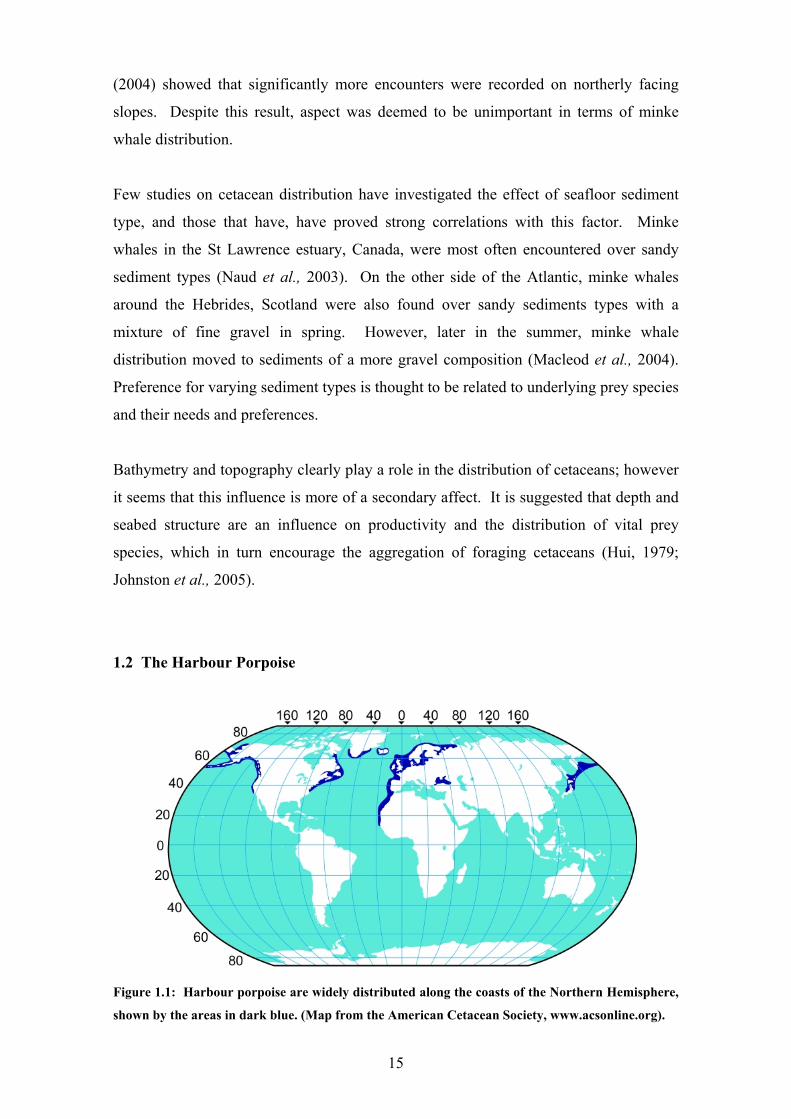
Figure 1.1: Harbour porpoise are widely distributed along the coasts of the Northern Hemisphere,
shown by the areas in dark blue. (Map from the American Cetacean Society, www.acsonline.org).
15

Harbour porpoise, Phocoena phocoena, is the most commonly known and studied
member of the Phocoena family. This species of small odontocete cetaceans inhabit the
continental shelf of temperate waters in the northern Hemisphere, shown in figure 1.1
(Johnston et al., 2005). Despite this virtually circumpolar navigation, animals from the
Pacific and Atlantic Ocean and Black Sea are all reproductively isolated from each
other (Bjorge & Tolley, 2004).
Harbour porpoise are small and robust, with an extremely thick blubber layer which
aids in reducing heat loss in their cold water habitats. Visually, harbour porpoise have a
dark dorsal side and a white ventral and despite their elusive behaviour are easily
distinguished from other cetaceans by their rounded head, absence of a beak and
triangular shaped dorsal fin (figures 1.2 and 1.3).
Figure 1.2: With a dark dorsal and white ventral side the porpoise is most clearly distinguished
from other coastal species by its triangular shapes dorsal fin. (Photograph by Kevin Robinson).
16

Black or dark dorsal side
Small rounded head with no beak
Wco
Figure 1.3: Illustration of the morpholog
phocoena).
Harbour porpoise have an averag
measures 65 to 70 cm and does not
fully grown porpoise exhibit slight
cm and 50 kg in weight and female
Sexual maturity occurs at 3-4 year
short lived species, the harbour por
Such reproductive cycles were desc
the Bay of Fundy by Gaskin et al.
followed by ovulation and concept
early autumn, most females examin
months, allowing females to give b
thought to occur for 8-12 months w
Lockyer, 1995; Read, 2000; Calder
North Sea and around the coast of W
June (Pierpoint et al., 1998).
Triangular shaped dorsal
hite or lighter loured ventral side
ical characteristics of the harbour porpoise (Phocoena
e life span of 8-10 years. At birth the porpoise
reach a maximum length until 8 years of age. Once
sexual dimorphism with males growing to 60-118
s growing to 66-118 cm and 55 kg (Lockyer, 1995).
s and to maximise reproductive success in such a
poise gives birth once a year (Gaskin et al., 1984).
ribed in harbour porpoise in the Gulf of Maine and
(1984). Parturition was observed to occur in May
ion in late June and early July. By late summer or
ed were pregnant. Gestation was estimated at 10.6
irth and conceive the following spring. Lactation is
hile the females are pregnant (Gaskin et al., 1984;
an, 2003). This coincides with observations in the
ales where juveniles were first sighted in May and
17

1.2.1 Diet
Due to their small size, harbour porpoise have a relatively high turnover of energy
reserves and low energy storage capacity (Brodie, 1995). This explains why an
estimated 3.5 % of the animal’s body weight in prey must be consumed daily, a figure
which increases by 80 % in lactating females (Yasui & Gaskin, 1986). The distribution
of harbour porpoise, therefore, is restricted to areas in close proximity to the distribution
of their prey (Santos & Pierce, 2003). Analysis of stomach contents of harbour
porpoise stranded and by-caught in UK waters revealed important prey species to
include; sandeels (Ammodytes marinus), gobies (Gobius sp.), whiting (Merlangius
merlangius), herring (Clupea harengis), poor cod (Trisopterus minutes), haddock
(Melanogrammus aeglefinus), Norway pout (Trisopterus esmarkii), and pollack
(Pollachius pollachius). Some of these prey species are displayed in figure 1.4
(Peirpoint et al., 1998; Pollock et al., 2000; Evans 1990).
A B
C
Figure 1.4: A number of prey species have been identified from the stomach contents of stranded
and by-caught harbour porpoise. 3 common species include A) the sandeel (Ammodytes marinus),
B) herring (Clupea harengis) and C) whiting (Merlangius merlangius). (Images from BBC, National
Geographic and fishnet respectively).
18
In Scottish waters sandeels are reported to be an important part of the diet in summer,
constituting 58 % of the stomach content (Payne et al., 1986), whilst other species such
as haddock, whiting, herring and pollack become more important during autumn and
winter when the availability of sandeels is thought to decline (Pollock et al., 2000). It
has also been suggested, that of these species, only the smaller individuals are
consumed by the harbour porpoise. This is thought to be due to the morphology of their
jaws, which can only gape to approximately 8 cm restricting the consumption of larger
fish (Calderan, 2003). Feeding behaviour of harbour porpoise includes logging at the
surface, often holding position in tidal races, surface lunges, changing direction abruptly
and loose aggregations of animals occurring periodically to allow cooperative foraging.
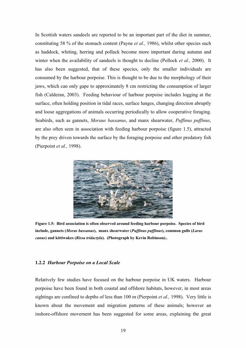
Seabirds, such as gannets, Moraus bassanus, and manx shearwater, Puffinus puffinus,
are also often seen in association with feeding harbour porpoise (figure 1.5), attracted
by the prey driven towards the surface by the foraging porpoise and other predatory fish
(Pierpoint et al., 1998).
Figure 1.5: Bird association is often observed around feeding harbour porpoise. Species of bird
include, gannets (Morus bassanus), manx shearwater (Puffinus puffinus), common gulls (Larus
canus) and kittiwakes (Rissa tridactyla). (Photograph by Kevin Robinson)..
1.2.2 Harbour Porpoise on a Local Scale
Relatively few studies have focused on the harbour porpoise in UK waters. Harbour
porpoise have been found in both coastal and offshore habitats, however, in most areas
sightings are confined to depths of less than 100 m (Pierpoint et al., 1998). Very little is
known about the movement and migration patterns of these animals; however an
inshore-offshore movement has been suggested for some areas, explaining the great
19
reduction in animals over the winter season (Jones, 2004; Calderan, 2003; Pierpoint et
al., 1998; Robinson et al., 2005). A number of studies based around the coast of Wales
found harbour porpoise to increase in numbers and aggregate during late summer and
early autumn, suggesting these waters to be an important coastal habitat for the species
at this time of year (Pierpoint et al., 1998; Jones, 2004). The relative abundance of
0.72 animals / km in the Welsh candidate for a Special Area of Conservation further
supports this proposition (Pierpoint et al., 1998).
The SCANS survey (1994) estimated harbour porpoise abundance of 341,366 in the
North Sea and adjacent waters. The SCANS survey area was divided into Blocks.
Block D encompassed part of the outer Moray Firth and was estimated to have a relative
abundance of 0.363 porpoise / km. This figure is significantly lower than other areas of
the SCANS survey, such as the coastal northern Wadden Sea where 0.812 porpoise / km
were calculated (Hammond et al., 1995). The first small-scale focal study on harbour
porpoise in the outer Moray Firth calculated the relative abundance to be 0.752 porpoise
/ km in 2003, a significant elevation from the SCANS survey result (Whaley, 2004).
This high relative abundance indicated the outer Moray Firth to have one of the highest
abundance levels yet recorded in the coastal waters of the UK, even greater than that
recorded in the candidate for a Special Area of Conservation in Wales.
1.2.3 Status
Harbour porpoise are widely distributed in the northern hemisphere, and are a
commonly sighted species in many coastal areas of Ireland and Britain (Weare, 2003).
However, in many areas harbour porpoise numbers have declined, such as the French
coast, English Channel, Baltic Sea and Southern North Sea, while other areas have seen
complete eradication of the species such as the Mediterranean Sea (Baines et al., 1997).
Harbour porpoise, like all cetaceans, are protected under UK and EU law. International
protection includes; listing under the 1992 EU Habitats and Species Directive under
Appendix II and IV, whereby the deliberate capture and killing of animals is prohibited.
Appendix II of CITES (Convention on International Trade in Endangered Species),
Appendix II of ASCOBANS (Agreement on the Conservation of Small Cetaceans of the
Baltic and North Seas) and the Bern Convention also offer protection. On a national
20
scale harbour porpoise are also protected under Schedule 5 of the Wildlife and
Countryside Act 1981 (UK Biodiversity Group, 1999) (Jones, 2004). To establish
protection of the harbour porpoise, the EU Habitats and Species Directive Annex II
requires Special Areas of Conservation to be set up in identified areas of physical and
biological importance to the life and reproduction of the harbour porpoise (EC, 1992;
Calderan, 2003). This year, the inner Moray Firth became a Special Area of
Conservation for the resident population of bottlenose dolphin and an area in west
Wales is currently a candidate for a Special Area of Conservation for the same species.
To date, however, no such area has been identified as highly important to harbour
porpoise due to the lack of knowledge on most aspects of their ecology, distribution and
habitat. (Weare, 2003). Understanding such factors is highly challenging due to their
wide distribution, seasonal migration, elusive behaviour, lack of distinctive
characteristics to allow identification of individuals and lack of studies concentrated on
this species (Calderan, 2003).
1.2.4 Threats
Between 1991 and 1993, 47 % of stranded cetaceans in Scotland were harbour porpoise
(Ross & Wilson, 1996) suggesting that these animals are faced with a great number of
threats in these waters. Evidence has indicated that harbour porpoise numbers have
declined in UK waters since the 1940s and suggested reasons for this include; incidental
capture in fishing gear, pollution and environmental change (Calderan, 2003). In
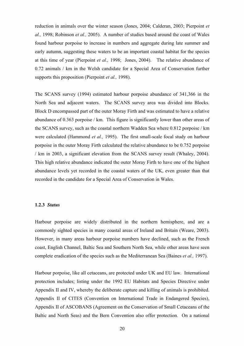
Wales, incidental by-catch has been identified as the greatest threat to harbour porpoise
(figure 1.6) and that threat is increasing. Kirkwood et al. (1997) proved that the
numbers of stranded harbour porpoise due to by-catch had increased each year between
1990 and 1995. A further significant threat to porpoise in Welsh waters is disturbance
from human activities, especially during the summer season when numbers of harbour
porpoise are greatest. Disturbance at this time is also highly problematic as it coincides
with the breeding period (Jones, 2004).
21
Figure 1.6: One of the greatest threats to harbour porpoise in the UK is from the fishing industry.
The threat of by-catch is increasing and is likely to be having a detrimental affect on the
population. (Images from the BBC and IFAW respectively).
Other threats identified in UK waters include; contaminants such as polychlorinated
biphenyls (PCBs) which increase infectious disease in the population, noise disturbance,
oil and gas exploration, interspecific interactions, in particular with bottlenose dolphins,
and increases in boat traffic (Pierpoint et al., 1998; Jones, 2004; Patterson et al., 1998).
Such threats contribute to the high level of mortality recorded in harbour porpoise with
50 % of animals not reaching the age of 4 years and a total annual mortality of 17 %
estimated in Scottish waters. This is likely to be detrimental to the population, as the
annual reproductive rate was calculated at only 8 % (Learmouth et al., 2005). As a
short lived species, that breeds annually it is likely that the harbour porpoise is already
maximising its rate of reproduction. It is vital, therefore, that these threats discussed are
severely reduced or eliminated to slow the decline of this species. Learmouth et al.
(2005) showed that, should the effect of interspecific interactions with bottlenose
dolphins be removed, the annual mortality would decline by 1 %, a significant
proportion for a threatened species.
1.3 Interspecific Interactions
A total of 227 stranded or by-caught harbour porpoise off the east coast of Scotland
were examined between 1990 and 2001, of these 227 animals, 61% revealed signs of
interspecific interactions with bottlenose dolphins (Wilson et al., 2004). Interactions
between the harbour porpoise and bottlenose dolphins were first identified in the Moray
Firth by Ross and Wilson (1996), where 42 out of 44 examined porpoise showed signs
22
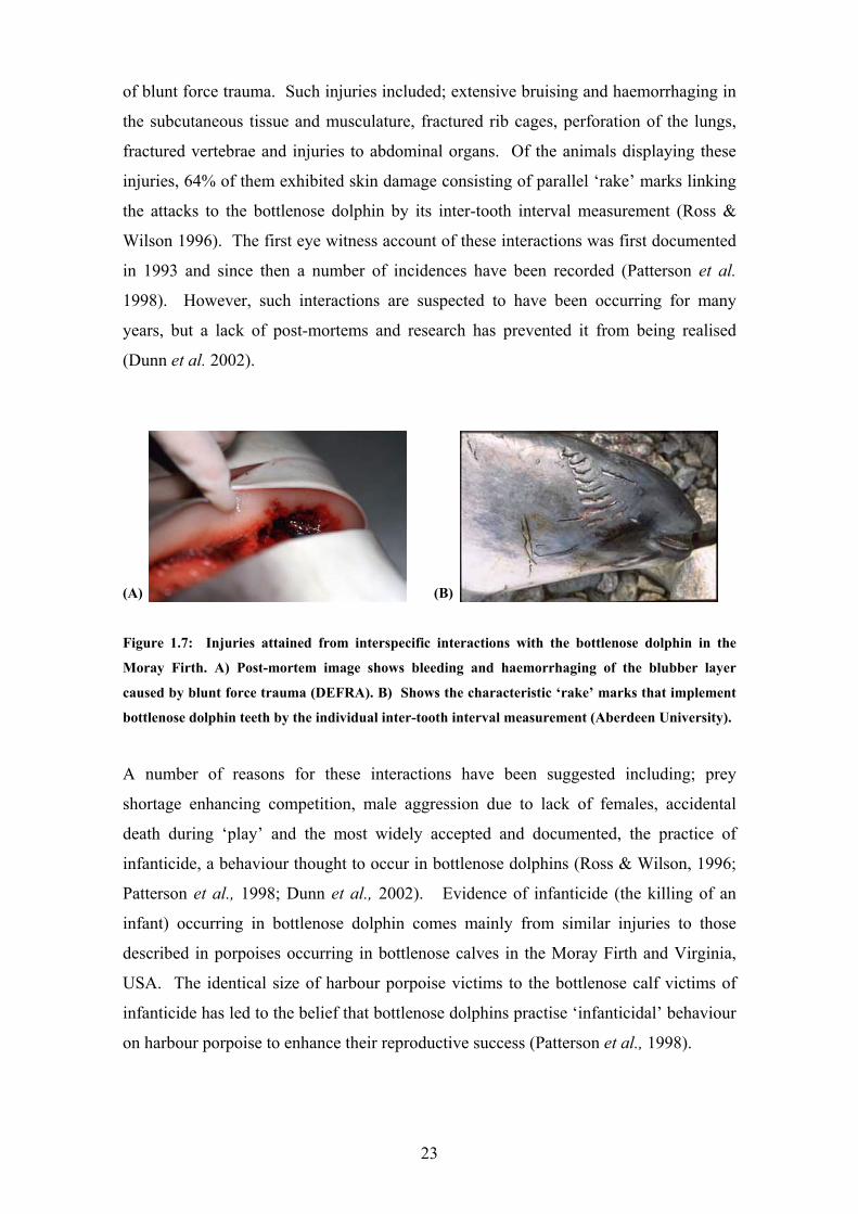
of blunt force trauma. Such injuries included; extensive bruising and haemorrhaging in
the subcutaneous tissue and musculature, fractured rib cages, perforation of the lungs,
fractured vertebrae and injuries to abdominal organs. Of the animals displaying these
injuries, 64% of them exhibited skin damage consisting of parallel ‘rake’ marks linking
the attacks to the bottlenose dolphin by its inter-tooth interval measurement (Ross &
Wilson 1996). The first eye witness account of these interactions was first documented
in 1993 and since then a number of incidences have been recorded (Patterson et al.
1998). However, such interactions are suspected to have been occurring for many
years, but a lack of post-mortems and research has prevented it from being realised
(Dunn et al. 2002).
(A) (B)
Figure 1.7: Injuries attained from interspecific interactions with the bottlenose dolphin in the
Moray Firth. A) Post-mortem image shows bleeding and haemorrhaging of the blubber layer
caused by blunt force trauma (DEFRA). B) Shows the characteristic ‘rake’ marks that implement
bottlenose dolphin teeth by the individual inter-tooth interval measurement (Aberdeen University).
A number of reasons for these interactions have been suggested including; prey
shortage enhancing competition, male aggression due to lack of females, accidental
death during ‘play’ and the most widely accepted and documented, the practice of
infanticide, a behaviour thought to occur in bottlenose dolphins (Ross & Wilson, 1996;
Patterson et al., 1998; Dunn et al., 2002). Evidence of infanticide (the killing of an
infant) occurring in bottlenose dolphin comes mainly from similar injuries to those
described in porpoises occurring in bottlenose calves in the Moray Firth and Virginia,
USA. The identical size of harbour porpoise victims to the bottlenose calf victims of
infanticide has led to the belief that bottlenose dolphins practise ‘infanticidal’ behaviour
on harbour porpoise to enhance their reproductive success (Patterson et al., 1998).
23
With bottlenose dolphins presenting a significant threat to the harbour porpoise in the
Moray Firth it is suspected that species partitioning occurs between the 2 species with
harbour porpoise avoiding areas where dolphins are present. In other areas of the world
species partitioning has been reported to be due to other factors such as prey
competition. In the northwest Atlantic, fin, humpback and minke whales were observed
to be segregated by depth to avoid direct competition for prey (Pollock et al., 2000).
1.4 Aims of the Study
In recent years, more and more demands have been placed on the conservation of
cetaceans in UK waters. As discussed above, the populations of harbour porpoise in the
UK are facing a great number of threats resulting in observed population declines and
an uncertain future. To effectively manage and conserve cetaceans, knowledge of their
spatial and temporal distribution is required on both large and small scales. For
example off the coast of California harbour porpoise were rarely found in depths greater
than 110m, whilst in contrast, near the San Juan Islands, they were frequently
encountered in depths greater than 100 m (Carretta et al., 2000). It is, therefore, clearly
important to examine defining variables on local scales. Identification of harbour
porpoise habitat preference will enhance our knowledge of the ecology and life history
of this species on a local scale, enabling greater awareness of population trends and
aiding in the establishment of marine protected areas (Macleod et al., 2004).
Therefore, the aim of this study is to analyse spatial and temporal trends of harbour
porpoise, Phocoena phocoena, in the outer Moray Firth and to highlight annual patterns
in distribution. Various techniques, including Geographical Information Systems (GIS),
will be used in the identification of preferred habitat types and factors affecting the
distribution of the harbour porpoise, which will greatly aid in the knowledge of the
ecology of this population and in identifying areas of importance for the species.
24
1.4.1 Summary of Aims
1) To highlight spatial trends in the distribution of harbour porpoise in the outer
Moray Firth. Variables include:
a. Depth
b. Slope gradient
c. Aspect
d. Sediment Type
2) To highlight the temporal patterns in harbour porpoise distribution. Analysis
within and between years and changes in group sizes are observed.
3) Interspecific interactions with bottlenose dolphins in the outer Moray Firth
are suspected to have a serious impact on harbour porpoise. In this section
the effect of bottlenose dolphins on porpoise distribution is examined.
25

2. The Study Area
26
2 The Study Area
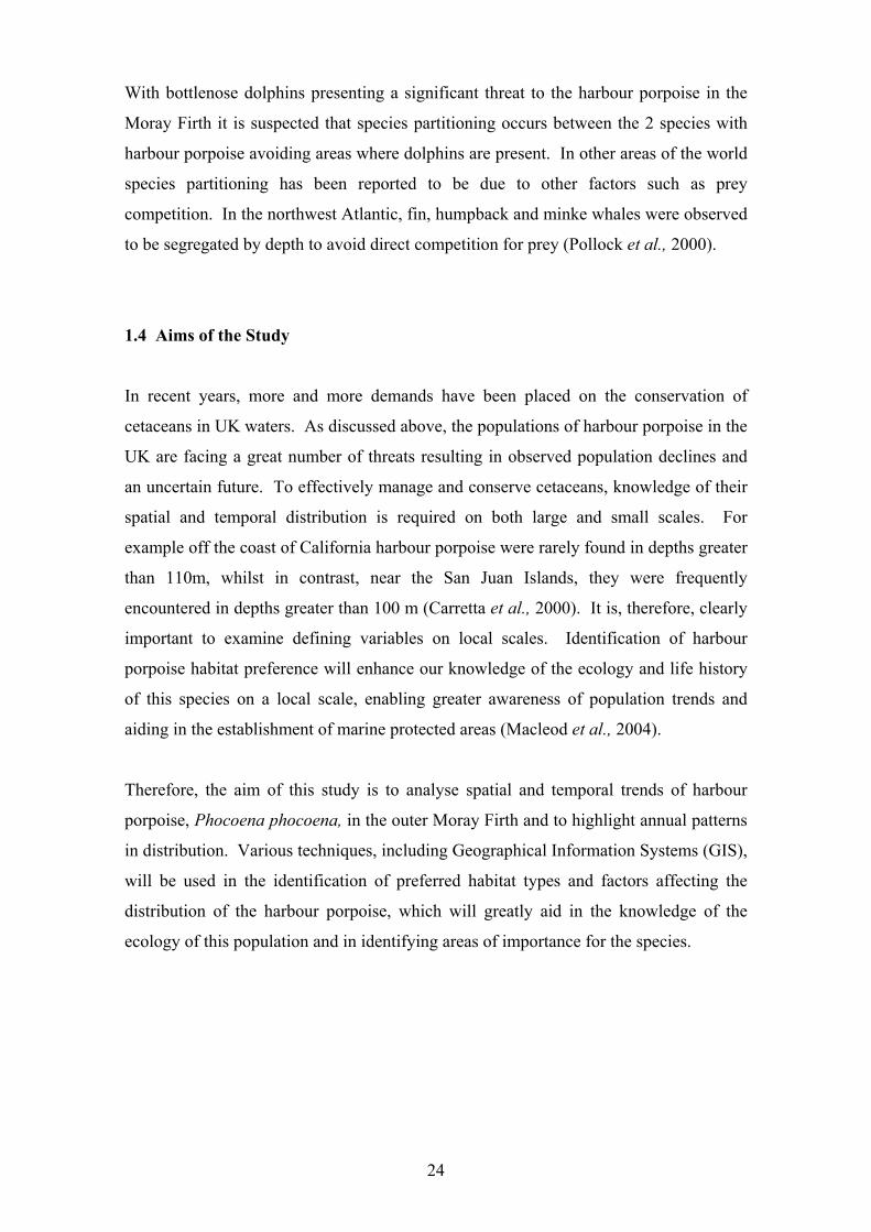
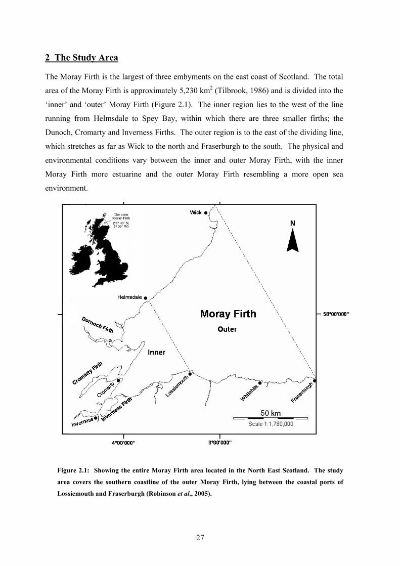
The Moray Firth is the largest of three embyments on the east coast of Scotland. The total
area of the Moray Firth is approximately 5,230 km2 (Tilbrook, 1986) and is divided into the
‘inner’ and ‘outer’ Moray Firth (Figure 2.1). The inner region lies to the west of the line
running from Helmsdale to Spey Bay, within which there are three smaller firths; the
Dunoch, Cromarty and Inverness Firths. The outer region is to the east of the dividing line,
which stretches as far as Wick to the north and Fraserburgh to the south. The physical and
environmental conditions vary between the inner and outer Moray Firth, with the inner
Moray Firth more estuarine and the outer Moray Firth resembling a more open sea
environment.
Fig
ar
Lo
ure 2.1: Showing the entire Moray Firth area located in the North East Scotland. The study
ea covers the southern coastline of the outer Moray Firth, lying between the coastal ports of
ssiemouth and Fraserburgh (Robinson et al., 2005).
27
The coastline of the outer Moray Firth is typically rugged and irregular, consisting of steep
cliffs, headlands, and small bays. The seabed topography in this area is also uneven,
dropping to depths of 60 m within only 5-10 km of the coast (Hardy-Hill, 1993). Depths
also fluctuate due to the presence of oceanographic structures, such as submarine banks,
and deep sea trenches (Wilson, 1996). The most prominent of these trenches is known as
the Southern Trench, located at the southeast side of the outer Moray Firth, only 7 km from
the coast, and can reach depths of up to 250 m. In contrast, the inner Firth coastline
consists of smooth mud or sandflats, sanddunes and cliffs, with seabed depths only reaching
50 m approximately 15 km from the shore (Admiralty Charts C22, 1997). The coastal
regions of the Moray Firth primarily consist of sand and gravel sediments, but an inverse
relationship between depth and gradient size is observed with finer, muddy sediments in
deeper, offshore waters (Reid and McManus, 1987).
As part of the wider North Sea basin, both coastal and mixed (coastal and oceanic) waters
occur in the Moray Firth (Adams, 1987). The main current influencing the Moray Firth is
the Dooleys Current, which brings mixed waters into the region from the north, which then
circulates in a clockwise direction inside the Moray Firth.
Temperature and salinity also vary both spatially and temporally in this northeast location.
The southern coast and inner Moray Firth are influenced greatly by the 12 major rivers
which run into the Firth. These rivers result in warmer temperatures in summer, colder
temperatures in winter, and reduced salinity in the inner part of the Firth. Subsequently
estuarine conditions decline with distance from the inner Moray Firth to more ‘mixed’
waters in the outer regions, where salinities exceed 34.8 and temperatures are generally
warmer in winter and colder in summer (Wilson, 1996).
The Moray Firth has long been regarded as an important area in terms of biodiversity and
productivity which has led to heavy utilisation by man. Such activities include fishing,
shipping, recreation and exploration for oil and gas. Fishing is an economically important
activity for the local communities. Some of the more important species include herring
(Clupea harengus), over wintering sprat (Sprattus sprattus), migrating mackerel (Scomber
scomber), sandeels (Ammodytes marinus), and Atlantic salmon (Salmosalnar) (Harding-
Hill, 1993). It is these species that support such a diverse range of seabirds and marine
mammals in the Moray Firth area. The most commonly encountered marine mammals are
the bottlenose dolphin (Tursiops truncatus), the harbour porpoise (Phocoena phocoena),
28

minke whale (Balaenoptera acutorostrata), grey seal (Halichoerus grypus) and common
seal (Phoca vitulina). In total 23 species of cetaceans have been recorded in Moray Firth
waters (Harding-Hill, 1993).
It is the presence of the bottlenose dolphin that has resulted in the inner Moray Firth being
awarded Special Area of Conservation (SAC) status. The European Commission Habitat
Directive demands the presence of conservation areas, in order to conserve the 189 habitat
types and 788 species in most need of protection, highlighted in Annexes I and II of the
Habitats Directive (JNCC 2005). The bottlenose dolphin is included in this category, as the
only known resident population of bottlenose dolphins in the North Sea, making the Moray
Firth one of only two known outstanding localities of this species in the UK.
29

3. Methods
30

3 Method
3.1 Data Collection
Figure 3.1: Staff and trained volunteers survey in one of the CRRU’s 5.4m RIBs (photo by Kevin
Robinson).
Data was collected during dedicated boat surveys carried out during the years of 2002
and 2005 and between the months of May and October, with the exception of October
2005 when no surveys were conducted. The survey vessels left from the harbour of
Whitehills, situated in the centre of an 880 km2 survey route. The survey route ran from
Lossiemouth in the west to Fraserburgh in the east between 4 designated waypoints.
The survey route was further divided into four different survey paths. The inner most
route labelled ‘Survey Route 1’. The other three survey routes were labelled 2, 3 and 4,
each separated by 45 minutes of longitude and situated progressively further from the
coastline (figure 3.2).
31

Figure 3.2: Showing the southern coastline of the outer Moray Firth and the survey routes used by the CRRU during systematic boat surveys between the ports of Fraserburgh and Lossiemouth. The transects are divided into 3 longitudinal outer routes (routes 2 to 4 respectively), each approximately 45 minutes apart in latitude, and an inner coastal route used during dedicated bottlenose dolphin surveys.
32
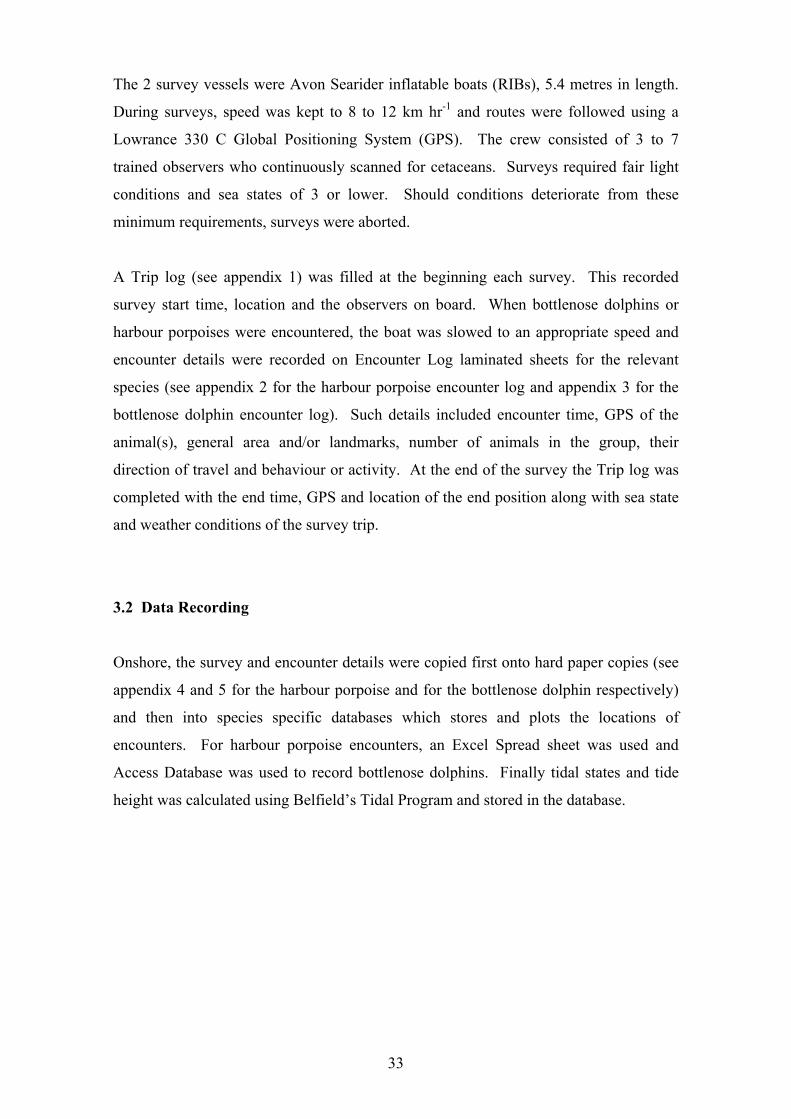
The 2 survey vessels were Avon Searider inflatable boats (RIBs), 5.4 metres in length.
During surveys, speed was kept to 8 to 12 km hr-1 and routes were followed using a
Lowrance 330 C Global Positioning System (GPS). The crew consisted of 3 to 7
trained observers who continuously scanned for cetaceans. Surveys required fair light
conditions and sea states of 3 or lower. Should conditions deteriorate from these
minimum requirements, surveys were aborted.
A Trip log (see appendix 1) was filled at the beginning each survey. This recorded
survey start time, location and the observers on board. When bottlenose dolphins or
harbour porpoises were encountered, the boat was slowed to an appropriate speed and
encounter details were recorded on Encounter Log laminated sheets for the relevant
species (see appendix 2 for the harbour porpoise encounter log and appendix 3 for the
bottlenose dolphin encounter log). Such details included encounter time, GPS of the
animal(s), general area and/or landmarks, number of animals in the group, their
direction of travel and behaviour or activity. At the end of the survey the Trip log was
completed with the end time, GPS and location of the end position along with sea state
and weather conditions of the survey trip.
3.2 Data Recording
Onshore, the survey and encounter details were copied first onto hard paper copies (see
appendix 4 and 5 for the harbour porpoise and for the bottlenose dolphin respectively)
and then into species specific databases which stores and plots the locations of
encounters. For harbour porpoise encounters, an Excel Spread sheet was used and
Access Database was used to record bottlenose dolphins. Finally tidal states and tide
height was calculated using Belfield’s Tidal Program and stored in the database.
33
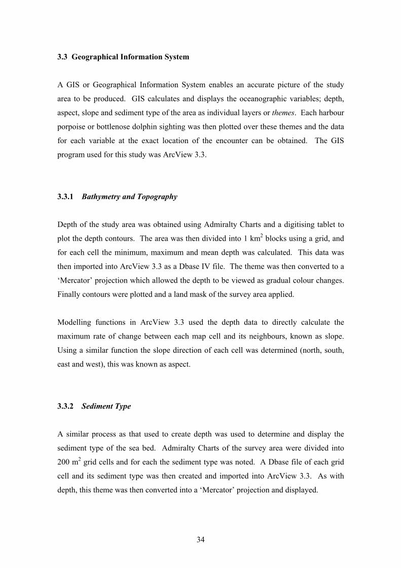
3.3 Geographical Information System
A GIS or Geographical Information System enables an accurate picture of the study
area to be produced. GIS calculates and displays the oceanographic variables; depth,
aspect, slope and sediment type of the area as individual layers or themes. Each harbour
porpoise or bottlenose dolphin sighting was then plotted over these themes and the data
for each variable at the exact location of the encounter can be obtained. The GIS
program used for this study was ArcView 3.3.
3.3.1 Bathymetry and Topography
Depth of the study area was obtained using Admiralty Charts and a digitising tablet to
plot the depth contours. The area was then divided into 1 km2 blocks using a grid, and
for each cell the minimum, maximum and mean depth was calculated. This data was
then imported into ArcView 3.3 as a Dbase IV file. The theme was then converted to a
‘Mercator’ projection which allowed the depth to be viewed as gradual colour changes.
Finally contours were plotted and a land mask of the survey area applied.
Modelling functions in ArcView 3.3 used the depth data to directly calculate the
maximum rate of change between each map cell and its neighbours, known as slope.
Using a similar function the slope direction of each cell was determined (north, south,
east and west), this was known as aspect.
3.3.2 Sediment Type
A similar process as that used to create depth was used to determine and display the
sediment type of the sea bed. Admiralty Charts of the survey area were divided into
200 m2 grid cells and for each the sediment type was noted. A Dbase file of each grid
cell and its sediment type was then created and imported into ArcView 3.3. As with
depth, this theme was then converted into a ‘Mercator’ projection and displayed.
34

3.3.3 Sightings
The longitudinal and latitudinal positions of each harbour porpoise and bottlenose
dolphin encounter were converted into decimal positions for importing into ArcView
3.3, using the equation:
degrees + (minutes / 60)
The converted positions of each species were then saved as a Dbase file and imported
into ArcView 3.3. Each sighting could subsequently be plotted in relation to the
physical factors of that exact position.
In order for clear presentation and statistical analysis, the depth, aspect, slope and
sediment types at each encounter location were then extracted using the grid analysis
function in ArcView 3.3. This enabled the variables common to each species to be
compared and statistically analysed.
Encounter density for each species could also be calculated by converting the sightings
data from an event theme to a grid theme and then to a ‘Mercator’ projection. The data
was then displayed as a series of colours representing the number of encounters
recorded in each individual grid cell over the 4 survey seasons 2002-2005.
3.4 SPUE
SPUE or sightings per unit effort was calculated for each of the 4 survey routes using
the equation:
SPUE = number of sightings
total survey effort
35
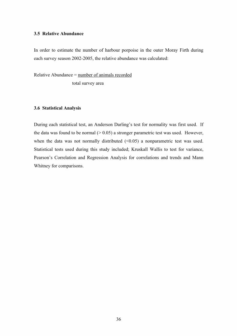
3.5 Relative Abundance
In order to estimate the number of harbour porpoise in the outer Moray Firth during
each survey season 2002-2005, the relative abundance was calculated:
Relative Abundance = number of animals recorded
total survey area
3.6 Statistical Analysis
During each statistical test, an Anderson Darling’s test for normality was first used. If
the data was found to be normal (> 0.05) a stronger parametric test was used. However,
when the data was not normally distributed (<0.05) a nonparametric test was used.
Statistical tests used during this study included; Kruskall Wallis to test for variance,
Pearson’s Correlation and Regression Analysis for correlations and trends and Mann
Whitney for comparisons.
36

4. Results
37
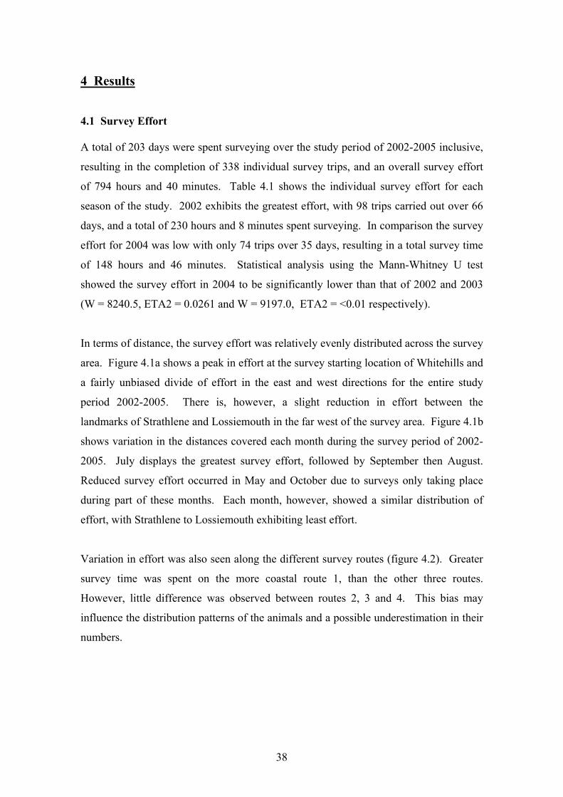
4 Results 4.1 Survey Effort A total of 203 days were spent surveying over the study period of 2002-2005 inclusive,
resulting in the completion of 338 individual survey trips, and an overall survey effort
of 794 hours and 40 minutes. Table 4.1 shows the individual survey effort for each
season of the study. 2002 exhibits the greatest effort, with 98 trips carried out over 66
days, and a total of 230 hours and 8 minutes spent surveying. In comparison the survey
effort for 2004 was low with only 74 trips over 35 days, resulting in a total survey time
of 148 hours and 46 minutes. Statistical analysis using the Mann-Whitney U test
showed the survey effort in 2004 to be significantly lower than that of 2002 and 2003
(W = 8240.5, ETA2 = 0.0261 and W = 9197.0, ETA2 = <0.01 respectively).
In terms of distance, the survey effort was relatively evenly distributed across the survey
area. Figure 4.1a shows a peak in effort at the survey starting location of Whitehills and
a fairly unbiased divide of effort in the east and west directions for the entire study
period 2002-2005. There is, however, a slight reduction in effort between the
landmarks of Strathlene and Lossiemouth in the far west of the survey area. Figure 4.1b
shows variation in the distances covered each month during the survey period of 2002-
2005. July displays the greatest survey effort, followed by September then August.
Reduced survey effort occurred in May and October due to surveys only taking place
during part of these months. Each month, however, showed a similar distribution of
effort, with Strathlene to Lossiemouth exhibiting least effort.
Variation in effort was also seen along the different survey routes (figure 4.2). Greater
survey time was spent on the more coastal route 1, than the other three routes.
However, little difference was observed between routes 2, 3 and 4. This bias may
influence the distribution patterns of the animals and a possible underestimation in their
numbers.
38

Table 4.1: Dedicated survey effort shown by number of survey days, number of survey trips and hours spend surveying for each of the four survey seasons 2002-2005 inclusive.
Survey Season Number of Survey Days
Number of Survey Trips
Number of Survey Hours:Minutes
2002 66 98 230:08
2003 60 80 226:07
2004 35 74 148:56
2005 42 86 189:30
Total 203 338 794:40
(a)
0
2
4
6
8
10
12
14
LOSSIEMOUTH
BOARS ROCK
KINGSTO
N
SPEY BAY
PORTGORDON
BUCKIE
STRATHLENE
FINDOCHTY
PORTK0CKIE
CULLEN
SUNNYSIDE
SANDEND
PORTSOY
WHITEHILLS
BANFF
MACDUFF
MELROSE
GAMRIE BAY
TROUPE HEAD
PENNAN
ABERDOUR BAY
ROSEHEARTY
SANDHAVEN
FRASERBURGH
Landmarks along survey route
% S
urve
y ef
fort
(dis
tanc
e)
(b)
0
1
2
3
4
5
LOSSIEMOUTH
BOARS ROCK
KINGSTON
SPEY BAY
PORTGORDON
BUCKIE
STRATHLENE
FINDOCHTY
PORTKN0CKIE
CULLEN
SUNNYSIDE
SANDEND
PORTSOY
WHITEHILLS
BANFF
MACDUFF
MELROSE
GAMRIE BAY
TROUPE HEAD
PENNAN
ABERDOUR BAY
ROSEHEARTY
SANDHAVEN
FRASERBURGH
Landmarks along Survey Route
% S
urve
y Ef
fort
(dis
tanc
e)
May June July August September October Figure 4.1: Dedicated survey effort in terms of distance along the survey area using landmarks along the coastline. Graph (a) shows the total survey effort over the seasons 2002-2005 inclusive while (b) shows this survey effort by month over the same survey period.
39

0
20
40
60
80
100
120
140
1 2 3 4
Survey Route
Surv
ey E
ffort
(hou
rs)
2002 2003 2004 2005
Figure 4.2: Survey effort in terms of time for each of the 4 survey routes for the different survey seasons.
4.2 Sightings and Encounters Between May and October 2002-2005, a total of 668 cetaceans were encountered; 63%
(n = 422) harbour porpoises and 11.5% (n = 76) bottlenose dolphins (Figure 4.3).
Minke whales were also frequently observed making up 25% of all encounters.
Rissso’s dolphins were also recorded during the study, classified as other cetaceans,
these encounters only made up 0.5% of all sightings. During each survey season, a
greater number of encounters occur with harbour porpoises than bottlenose dolphins.
Despite a greater number of encounters, the total number of individual harbour
porpoises seen in 2004 and 2005 was less than the total number of bottlenose dolphins.
2002-2005 inclusive recorded 1138 harbour porpoises and 900 bottlenose dolphins
(table 4.2).
harbour porpoise bottlenose dolphin minke whale other cetacean Figure 4.3: Harbour porpoise, bottlenose dolphins and minke whales are the three most commonly sighted cetaceans in the survey area between May and October 2002-2005 inclusive. The other cetaceans observed were risso’s dolphins.
40
Figure 4.4 shows the encounters of harbour porpoises and bottlenose dolphins with time
spent surveying during each season of the study. The pattern of encounters by season
for each of the two species is very different. A decline in harbour porpoise from 2002
to 2004 is shown, with only a slight increase in encounters during 2005. The reduced
survey effort in 2004 can only partly explain this decline (figure 4.4a). Bottlenose
dolphin encounters show a more irregular pattern, with an increase in encounters from
2002 to 2003, without any increase in survey effort. Encounters decreased highly
significantly in 2004, partly explained by the reduced survey effort. The survey effort
increased in 2005 and with it a significant increase in encounters (figure 4.4b).
41

Table 4.2: Encounters of harbour porpoise and bottlenose dolphin during each of the four field seasons 2002-2005 and the total number of animals for each
species encountered during this time
Number of Encounters Total Number of Animals Survey Season
Harbour porpoise
Bottlenose dolphin Harbour porpoise Bottlenose dolphin
2002 169 15 415 148
2003
137 20 461 240
2004 53 9 117 179
2005 65 32 145 333
Total 422 67 1138 900
42

(a)
0
50
100
150
200
250
2002 2003 2004 2005
Survey Season
Sur
vey
effo
rt (h
ours
)
0
5
10
15
20
25
30
35
40
45
% h
arbo
ur p
orpo
ise
enco
unte
rs
Survey effort (time) % harbour porpoise encounters (b)
0
50
100
150
200
250
2002 2003 2004 2005
Survey Season
Sur
vey
Effo
rt (h
ours
)
0
5
10
15
20
25
30
35
40
45
% b
ottle
nose
dol
phin
enc
ount
ers
Survey Effort (time) % bottlenose dolphin encounters
Figure 4.4: Survey effort in terms of time (hours) for each of the four survey seasons 2002-2005 inclusive plotted for (a) the number of harbour porpoises and (b)
the number of bottlenose dolphins encountered during the survey period.
43

4.3 Harbour Porpoise on a Spatial Scale
37
42
47
1.752.002.252.502.753.003.25
Longitude W
Latit
ude
57o N 50 m100 m
200 m
20 m
Figure 4.5: Plot shows the location of all harbour porpoise encounters during the study period of May to October 2002-2005 inclusive. Green dots indicate the
major towns along the coastline of the survey area and 20 m, 50 m, 100 m and 200 m depth contours are also displayed.
44

Harbour porpoises are encountered across the entire study area from Lossiemouth in the
west to Fraserburgh in the east. Figure 4.5 shows harbour porpoise to be most often
observed close to shore between the towns of Rosehearty and Buckie in water depths of
around 20 m. However a fairly significant number of encounters were also observed in
deeper, more offshore waters in depths up to 150 m.
Figure 4.5 does not reflect the distribution of survey effort which may influence the
perception of harbour porpoise distribution over the survey area. Figure 4.6 displays the
proportion of harbour porpoise encounters alongside the amount of effort spent on each of
the four survey routes (1-4). Most effort was spent on the coastal survey route number 1,
which resulted in only 30% of the harbour porpoise encounters. Less than half this effort
was spent on the 2nd survey route, however, a greater number of encounters were recorded
(34%). Survey routes 3 and 4 exhibited progressively less effort and with it fewer
encounters, 23% and 14% respectively.
0:00:00
48:00:00
96:00:00
144:00:00
192:00:00
240:00:00
288:00:00
336:00:00
384:00:00
432:00:00
480:00:00
1 2 3 4
Survey Route
Surv
ey E
ffort
(tim
e)
0
5
10
15
20
25
30
35
40
% h
arbo
ur p
orpo
ise
enco
unte
rs
Figure 4.6: Dedicated survey effort in terms of time and number of encounters by survey route for
each survey season 2002-2005. The four survey routes are labelled 1 – 4. Survey route 1 is closest to
the coast and 2-4 are progressively further offshore.
SPUE (sightings per unit effort) of harbour porpoise was calculated for each of the four
survey routes from the number of encounters recorded and the effort spent on each route
(table 4.3). Survey route 4 is located furthest from shore, and exhibited the highest SPUE
at 0.9 sightings / hour. The harbour porpoise SPUE declined with decreasing distance from
45

shore with the coastal survey route (1) displaying the lowest value. This trend suggests that
a greater number of harbour porpoise would be encountered in deeper, more offshore
waters if the survey effort on these routes was increased. This further indicated that the
number of harbour porpoise recorded in this study area is likely to be an underestimation of
the true numbers of harbour porpoise in the study area of the outer Moray Firth.
Table 4.3: SPUE (sightings per unit effort) of harbour porpoise calculated for each of the 4 survey
routes over the entire study period.
Survey Route Time No. of harbour
porpoise encounters
SPUE
No. sightings/ hour
1 432:59 121 0.28
2 173:43 142 0.82
3 114:14 98 0.86
4 66:45 61 0.9
The distribution of effort across the different survey routes has been shown to influence the
locations and numbers of harbour porpoise encounters. The sea state during individual
surveys is also shown to influence the probability of encountering porpoise. Harbour
porpoise are particularly susceptible to this bias due to their small size and elusive
behaviour towards boats. Figure 4.7 shows that the proportion of harbour porpoise
encounters declines with increasing sea state up to Beaufort Scale 5, when no survey trips
were carried out.
0
5
10
15
20
25
30
35
40
45
0 1 2 3 4 5
Sea State (Beauford Scale)
Pro
port
ion
of h
arbo
ur p
orpo
ise
enco
unte
rs
0
5
10
15
20
25
30
35
40
Pro
port
ion
on S
urve
y Tr
ips
% HP Encounters % Survey Trips
Figure 4.7: Proportions of harbour porpoise encounters and survey trips carried out during the study
period at varying sea states.
46
4.3.1 Geographical Information System
ArcView 3.3 was used to create and display the oceanographic structure of the survey area
using the variables depth, aspect, slope, and sediment type. Figure 4.8 shows the GIS
layouts for each variable. Depth along the coastline is shallow only reaching about 20 m
within few hundred metres of shore. The west side of the survey area, particularly Spey
Bay region, remains shallow only reaching 50 m in depth 15 km from the coast. In
contrast, the east side of the survey area shows larger depth gradients as depths reach over
100 m within only 8 km of the shore around the oceanographic feature of the ‘Southern
Trench’. Slope gradients are high in all areas of the survey with the exception of the
shallower Spey Bay. The inshore slopes predominantly face north. Further offshore,
principally around the Southern Trench, the aspect is highly variable. Along the coastline
sediment types vary from sand and gravel in Spey Bay to sandy gravel along the rest of the
coastline. Offshore sea beds consist of finer grains of sandy sediments and mud.
47

(A)
0 - 1919 - 3838 - 5757 - 7676 - 9595 - 114114 - 133133 - 151151 - 170Land
(B)
################################################################################################################################################################################################################################################################################################################################ ################################################################################################################################################################################### ############################################################################################################################################# ################################################################################################################################################################################################################################################################################################################################ ################################################################################################################################################################################################################################################################################################################################ ########################################################################################################################################################################################################################### ##################################################################################################### ################################################################################################################################################################################################################################################################################################################################ ################################################################################################################################################################################################################################################################################################################################ ################################################################################################################################################################################################################################################################## ############################################################## ################################################################################################################################################################################################################################################################################################################################ #################################################################################################################################################################################################################################################################################################################################
)
(C)
(D)
Figure 4.8: Fixed environmental variables of the survey area, Lossiemouth to Fraserburgh. Depth (A
of slope (B), aspect of slope (C) and sediment type of the seabed (D) and displayed and calculated using
3.3. 20 metre depth contours are also displayed.
48
Slope (degrees)
p0 - 1010 - 2020 - 2929 - 3939 - 4949 - 5959 - 6969 - 7979 - 88Land
MSMSSSGGRL
), gr
Ar
Aspect
SouthSouthwestWestNorthwestNorthNortheastEastSoutheastLand
t
SedimenDepth (meters
udandy mududdy sandandlightly gravelly sandandy gravelravelravelly sandockand
adient
cView

4.3.2 Harbour Porpoise Encounter Frequency
00 - 22 - 44 - 55 - 77 - 99 - 1111 - 1313 - 1414 - 16Land
Figure 4.9: The encounter density of harbour porpoise within the survey area. Map was constructed
using the interpolate function in ArcView 3.3.
The encounter frequency of harbour porpoise is generally concentrated along the coast up
to depths of 50 m (figure 4.9). There is an obvious lack of encounters in the Spey Bay area
with only a few encounters distributed further offshore. A concentration of encounters
occurred at Whitehills, where 14-16 encounters were recorded. This encounter ‘hotspot’
can be partly explained by the high survey effort in this location.
ArcView 3.3 was used to extract the harbour porpoise encounters along with specific data
for each of the 4 variables, depth, aspect, slope and sediment type at each sighting location
(figure 4.10). Observations of harbour porpoise increased with depth from a minimum of
6.86 m to 40 m, after which observations declined with depth up to 70 m. Above 70 m,
only a few encounters were recorded in each depth category up to the maximum depth of
145.62 m. Encounters increased with gradient of slope (mean 74.1˚) and were recorded on
all slope aspects (0-360˚) with significantly higher numbers on those facing north and
south. The sediment type at the majority of encounter locations was sandy gravel although
harbour porpoise were recorded at least once in areas consisting of each of the 9 sediment
types.
49

(A)
0
20
40
60
80
100
120
140
0-10
10-20
20-30
30-40
40-50
50-60
60-70
70-80
80-90
90-10
0
100-1
10
110-1
20
120-1
30
130-1
40
Depth (metres)
Harb
our p
orpo
ise
Enco
unte
r Fre
quen
cy
(B)
020
406080
100120140
160180
North
Northea
stEast
Southeas
t
South
Southwes
tWest
Northwes
t
Aspect
Harb
our p
orpo
ise
Enco
unte
r Fre
quen
cy
(C)
0
20
40
60
80
100
120
140
160
180
200
0-10 10-20 20-30 30-40 40-50 50-60 60-70 70-80 80-90
Slope (degrees)
Harb
our p
orpo
ise
Enco
unte
r Fre
quen
cy
(D)
050
100150200250300350
Mud
Sandy M
ud
Muddy S
and
Sandy M
ud
Slightly
Grave
lly San
d
Sandy G
ravel
Gravel
Gravell
y Sand
Rock
Sediment Type
Harb
our p
orpo
ise
Enco
unte
r Fr
eque
ncy
Figure 4.10: Encounter frequency of harbour porpoise with the environmental variables depth, aspect,
slope and sediment type.
The data was statistically analysed for trends and correlations using Kruskall Wallis to test
for variance (table 4.4) and Pearson’s Correlation and Regression analysis to further test
these relationships. Each variable displayed significant variance with harbour porpoise
encounter frequency. However, only depth and slope were calculated to have a significant
relationship with encounter frequency by Pearson’s Correlation. Depth was shown to have
a negative correlation = -0.578, P-value = 0.030 and slope to have a positive correlation,
Pearson’s Correlation = 0.781, P-value = 0.01. Aspect and sediment type showed no such
relationship. Despite a significant correlation, the regression analysis indicates the
relationship with depth and slope to not be functional suggesting other factors to be further
influencing their relationship with harbour porpoise encounter frequency (R2 = 0.3692 and
R2 = 0.5629 respectively).
50
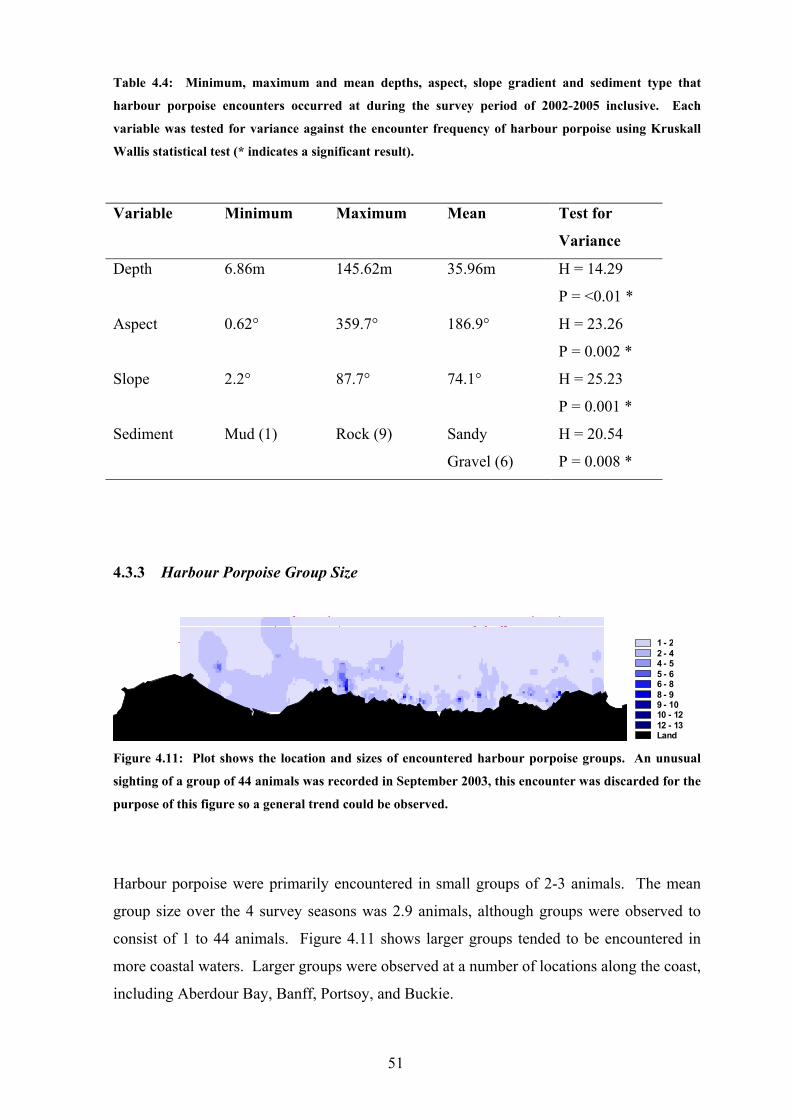
Table 4.4: Minimum, maximum and mean depths, aspect, slope gradient and sediment type that
harbour porpoise encounters occurred at during the survey period of 2002-2005 inclusive. Each
variable was tested for variance against the encounter frequency of harbour porpoise using Kruskall
Wallis statistical test (* indicates a significant result).
4.3.3 Harbour Porpoise Group Size
1 - 22 - 44 - 55 - 66 - 88 - 99 - 1010 - 1212 - 13Land
Variable Minimum Maximum Mean Test for
Variance
Depth 6.86m 145.62m 35.96m H = 14.29
P = <0.01 *
Aspect 0.62° 359.7° 186.9° H = 23.26
P = 0.002 *
Slope 2.2° 87.7° 74.1° H = 25.23
P = 0.001 *
Sediment Mud (1) Rock (9) Sandy
Gravel (6)
H = 20.54
P = 0.008 *
Figure 4.11: Plot shows the location and sizes of encountered harbour porpoise groups. An unusual
sighting of a group of 44 animals was recorded in September 2003, this encounter was discarded for the
purpose of this figure so a general trend could be observed.
Harbour porpoise were primarily encountered in small groups of 2-3 animals. The mean
group size over the 4 survey seasons was 2.9 animals, although groups were observed to
consist of 1 to 44 animals. Figure 4.11 shows larger groups tended to be encountered in
more coastal waters. Larger groups were observed at a number of locations along the coast,
including Aberdour Bay, Banff, Portsoy, and Buckie.
51
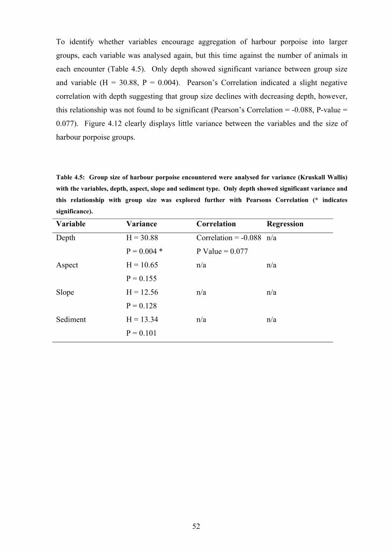
To identify whether variables encourage aggregation of harbour porpoise into larger
groups, each variable was analysed again, but this time against the number of animals in
each encounter (Table 4.5). Only depth showed significant variance between group size
and variable (H = 30.88, P = 0.004). Pearson’s Correlation indicated a slight negative
correlation with depth suggesting that group size declines with decreasing depth, however,
this relationship was not found to be significant (Pearson’s Correlation = -0.088, P-value =
0.077). Figure 4.12 clearly displays little variance between the variables and the size of
harbour porpoise groups.
Table 4.5: Group size of harbour porpoise encountered were analysed for variance (Kruskall Wallis)
with the variables, depth, aspect, slope and sediment type. Only depth showed significant variance and
this relationship with group size was explored further with Pearsons Correlation (* indicates
significance).
Variable Variance Correlation Regression
Depth H = 30.88
P = 0.004 *
Correlation = -0.088
P Value = 0.077
n/a
Aspect H = 10.65
P = 0.155
n/a n/a
Slope H = 12.56
P = 0.128
n/a n/a
Sediment H = 13.34
P = 0.101
n/a n/a
52

(A)
0
1
2
3
4
5
6
7
8
0-10
10-20
20-30
30-40
40-50
50-60
60-70
70-80
80-90
90-10
0
100-1
10
110-1
20
120-1
30
130-1
40
140-1
50
Depth
Ave
rage
har
bour
por
pois
e gr
oup
size
(B)
0
5
10
15
20
25
N NE E SE S SW W NW
Aspect of Slope
Ave
rage
har
bour
por
pois
e gr
oup
size
(C)
0
5
10
15
20
25
30
35
40
0-10 10-20 20-30 30-40 40-50 50-60 60-70 70-80 80-90
Slope (degrees)
Ave
rage
har
bour
por
pois
e gr
oup
size
(D)
0
5
10
15
20
25
Mud
Sandy
Mud
Muddy
sand
Sand
Slightl
y grav
elly s
and
sand
y grav
el
grave
l
grave
lly sa
ndroc
k
Sediment Type
Ave
rage
har
bour
por
pois
e gr
oup
size
Figure 4.12: Varying average group sizes of harbour porpoise with the variables depth, aspect, slope
and sediment type. Error bars show the variation of group sizes in each category.
4.4 Harbour Porpoise on a Temporal Scale
4.4.1 Harbour porpoise encounter frequency
Harbour porpoise were encountered 422 times over the 4 survey seasons and encounters
were recorded in all months with the exception of May 2005 (Table 4.6). The number of
encounters recorded in a month range from 1 in May and October 2004 up to 59 encounters
in September 2002. In 2002 and 2005, harbour porpoise sightings peaked in September at
59 and 20 encounters respectively, whilst in 2003 and 2004 this peak occurred in July. In
general over the 4 survey seasons, encounters were noted to increase from May to a peak in
July, a slight drop during August before a second peak in September (figure 4.13). The
variance between these two factors was found to be statistically significant (H = 13.33 DF
= 5 P = 0.021). The number of encounters also ranged significantly between the survey
seasons, from 169 in 2002 to a low of 53 in 2004 although this variance was not found to be
significant.
53
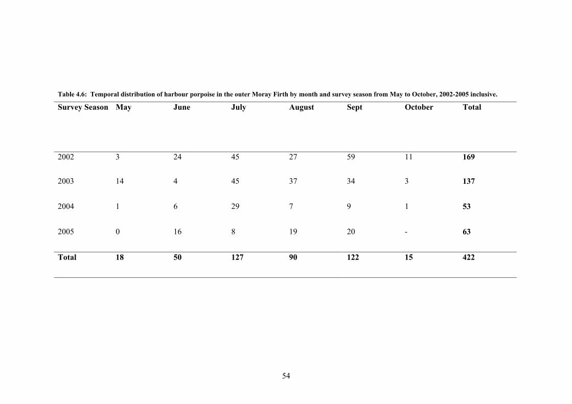
Table 4.6: Temporal distribution of harbour porpoise in the outer Moray Firth by month and survey season from May to October, 2002-2005 inclusive.
Survey Season May June July August Sept October Total
2002 3 24 45 27 59 11 169
2003
14 4 45 37 34 3 137
2004 1 6 29 7 9 1 53
2005 0 16 8 19 20 - 63
Total 18 50 127 90 122 15 422
54

0
20
40
60
80
100
120
140
May June July August September
Month
Enco
unte
r fr
eque
ncy
of h
arbo
ur
porp
oise
Figure 4.13: Frequency of harbour porpoise encounters varies through the season. Number of
encounters is shown over the months of May to September inclusive.
The distribution of harbour porpoise encounters was displayed and visually analysed by
month and survey season using ArcView 3.3. The distribution across survey season 2002-
2005 was highly variable and showed no trends. 2002 showed widely distributed
encounters with some concentration between Portknockie and Whitehills. 2003 showed a
more uneven distribution with encounters concentrated between Portsoy and Rosehearty.
2004 showed significantly fewer sightings but widely distributed. Finally 2005 showed
sightings to be more restricted to areas west of Cullen. Figure 4.14 shows the distribution
of encounters through the season of 2002 by month. Encounters are observed to be widely
distributed during May to July before moving further inshore and becoming more clustered
during the month of August. This pattern was not observed in any other survey season, nor
was any other pattern observed.
55

May
#
#
#
June
##
####
## #
##
###
##
#
#
###
##
#
July
#
###
###
# ##
#
##
# # #
#
### #### #
#
#
###
##
#
###
#
###
## #
##
August
# #
#
##
#
## ### ###
#### #
## ## ####
September
##### # ###
# #### # ##
######
#### #
####
###
###
##
#
# ####
## #
###
#
#
##
##
#
October
###
##
####
##
Figure 4.14: Monthly sightings of harbour porpoise during the survey season of 2002 (May to
October). Sightings were displayed with depth (deeper water represented by darker blue) using
ArcView 3.3.
56

Table 4.7: Relative abundance of harbour porpoise calculated for each of the 4 survey seasons (2002-
2005) for the outer Moray Firth. The outer Moray Firth has a calculated survey area of 550km2.
Survey Season No. of harbour
porpoise
Relative Abundance
(No. of animals / km2)
2002 415 0.75
2003 461 0.84
2004 117 0.21
2005 145 0.26
The number of animals encountered over the study period followed a similar pattern to that
of the number of encounters by survey season, with the exception that more individual
animals were observed in 2003 than 2002. Using this data, the relative abundance of
harbour porpoise in the outer Moray Firth can be estimated (table 4.7). A high relative
abundance was calculated for 2002 at 0.75 animals / km2. This figure increased to 0.84
animals / km2 in 2003 before declining significantly in 2004 to only 0.21 animals / km2 and
only increasing a little in 2005 to 0.26 animals / km2.
Tidal state during harbour porpoise encounters varied only slightly. Similar proportions
(20-25%) of harbour porpoise observations occurred during low, high and falling tides.
Increases in encounters were recorded during rising tides at 32%. This increase in
sightings can be explained by the increase in survey effort during this tidal state (figure
4.15).
0
5
10
15
20
25
30
35
Low High Falling Rising
Tidal State
Prop
ortio
n of
Sur
vey
Effo
rt
0
5
10
15
20
25
30
35
Prop
ortio
n of
har
bour
por
pois
e en
coun
ters
Survey Effort Harbour porpoise
Figure 4.15: Proportions of harbour porpoise encounters over the 4 tidal states; low, high, falling and
rising. Encounters were plotted along with survey effort distribution over these tidal states.
57
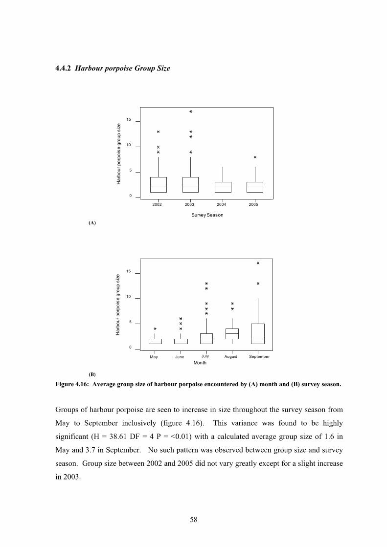
4.4.2 Harbour porpoise Group Size
(A)
2002 2003 2004 2005
0
5
10
15
Survey Season
Har
bour
por
pois
e gr
oup
size
(B)
May June July August September
0
5
10
15
Month
Har
bour
por
pois
e gr
oup
size
Figure 4.16: Average group size of harbour porpoise encountered by (A) month and (B) survey season.
Groups of harbour porpoise are seen to increase in size throughout the survey season from
May to September inclusively (figure 4.16). This variance was found to be highly
significant (H = 38.61 DF = 4 P = <0.01) with a calculated average group size of 1.6 in
May and 3.7 in September. No such pattern was observed between group size and survey
season. Group size between 2002 and 2005 did not vary greatly except for a slight increase
in 2003.
58
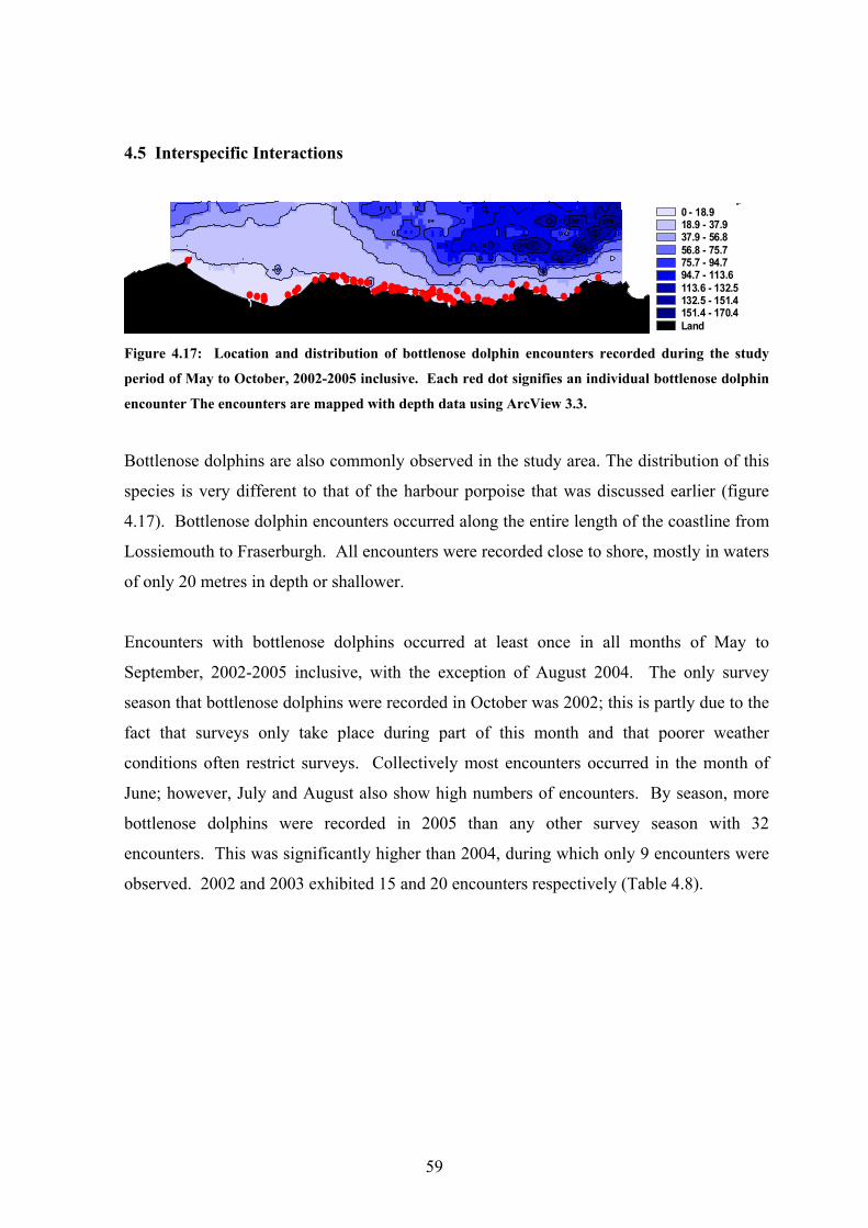
4.5 Interspecific Interactions
p0 - 18.918.9 - 37.937.9 - 56.856.8 - 75.775.7 - 94.794.7 - 113.6113.6 - 132.5132.5 - 151.4151.4 - 170.4Land
#
## ##
##
## # ### #
##
####
##
#
#
# ## # ## #
###
##
#
##
#
### ##
####
#
###
## #
#
#
###
#
### ###
###
###
#
#
Figure 4.17: Location and distribution of bottlenose dolphin encounters recorded during the study
period of May to October, 2002-2005 inclusive. Each red dot signifies an individual bottlenose dolphin
encounter The encounters are mapped with depth data using ArcView 3.3.
Bottlenose dolphins are also commonly observed in the study area. The distribution of this
species is very different to that of the harbour porpoise that was discussed earlier (figure
4.17). Bottlenose dolphin encounters occurred along the entire length of the coastline from
Lossiemouth to Fraserburgh. All encounters were recorded close to shore, mostly in waters
of only 20 metres in depth or shallower.
Encounters with bottlenose dolphins occurred at least once in all months of May to
September, 2002-2005 inclusive, with the exception of August 2004. The only survey
season that bottlenose dolphins were recorded in October was 2002; this is partly due to the
fact that surveys only take place during part of this month and that poorer weather
conditions often restrict surveys. Collectively most encounters occurred in the month of
June; however, July and August also show high numbers of encounters. By season, more
bottlenose dolphins were recorded in 2005 than any other survey season with 32
encounters. This was significantly higher than 2004, during which only 9 encounters were
observed. 2002 and 2003 exhibited 15 and 20 encounters respectively (Table 4.8).
59
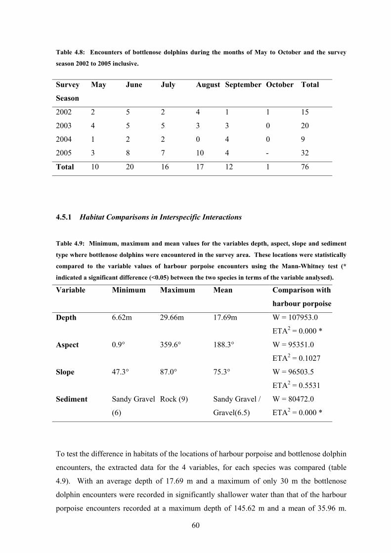
Table 4.8: Encounters of bottlenose dolphins during the months of May to October and the survey
season 2002 to 2005 inclusive.
Survey
Season
May June July August September October Total
2002 2 5 2 4 1 1 15
2003 4 5 5 3 3 0 20
2004 1 2 2 0 4 0 9
2005 3 8 7 10 4 - 32
Total 10 20 16 17 12 1 76
4.5.1 Habitat Comparisons in Interspecific Interactions
Table 4.9: Minimum, maximum and mean values for the variables depth, aspect, slope and sediment
type where bottlenose dolphins were encountered in the survey area. These locations were statistically
compared to the variable values of harbour porpoise encounters using the Mann-Whitney test (*
indicated a significant difference (<0.05) between the two species in terms of the variable analysed).
Variable Minimum Maximum Mean Comparison with
harbour porpoise
Depth 6.62m 29.66m 17.69m W = 107953.0
ETA2 = 0.000 *
Aspect 0.9° 359.6° 188.3° W = 95351.0
ETA2 = 0.1027
Slope 47.3° 87.0° 75.3° W = 96503.5
ETA2 = 0.5531
Sediment Sandy Gravel
(6)
Rock (9) Sandy Gravel /
Gravel(6.5)
W = 80472.0
ETA2 = 0.000 *
To test the difference in habitats of the locations of harbour porpoise and bottlenose dolphin
encounters, the extracted data for the 4 variables, for each species was compared (table
4.9). With an average depth of 17.69 m and a maximum of only 30 m the bottlenose
dolphin encounters were recorded in significantly shallower water than that of the harbour
porpoise encounters recorded at a maximum depth of 145.62 m and a mean of 35.96 m.
60

This difference in depth between the 2 species was found to be highly significant using
Mann Whitney statistical analysis (W = 107953.0 ETA2 = <0.01). The sediment type at
bottlenose dolphin and harbour porpoise encounters was also found to be significantly
different (W = 80472.0 ETA2 = <0.01) despite the mean sediment type for both species
being sandy gravel. Encounters of harbour porpoise were recorded at least once on each
sediment type compared to the bottlenose dolphin which was restricted to sandy gravel,
gravel, gravely sand and rock. Slope and aspect of the encounter locations were fairly
similar between the 2 species. Mean of encounters for both species was over south facing
slopes, however harbour porpoise encounters occurred over all slope directions, north to
south and east to west. Slope gradient for the 2 species was also comparable with only a
degree of difference between the 2 means and the maximum of 87.0˚ for the bottlenose
dolphin and 87.7˚ for the harbour porpoise. The only difference being that harbour
porpoise are also found at lower gradients compared to the bottlenose dolphin with
minimum values of 2.2˚ and 47.3˚ respectively.
Due to the recent documentation about the interactions between these 2 species, the
encounter frequency of the bottlenose dolphin was also used as a factor influencing the
distribution of the harbour porpoise. Figure 4.18 shows bottlenose dolphin encounter
frequency mapped using ArcView 3.3 which ranges from 0 to nearly 3 encounters. Areas
of high encounters, shown by dark blue, are located in Spey Bay, Portsoy, Whitehills, and
Banff.
61

4.5.2 Harbour porpoise Encounter Frequency
00.1 - 0.30.3 - 0.60.6 - 11 - 1.31.3 - 1.61.6 - 1.91.9 - 2.22.2 - 2.52.5 - 2.9Land
Figure 4.18: Encounter density of bottlenose dolphins within the survey area of the outer Moray
Firth. Map constructed using the interpolate function in ArcView 3.3 where white / light blue
represents none or few encounters and dark blue high numbers of encounters.
As with depth, slope, aspect and sediment variables, bottlenose dolphin encounter
frequency (figure 4.18) was statistically analysed against the encounter frequency of
harbour porpoise. Kruskall Wallis indicated there to be significant variance between
these 2 factors (H = 32.46 DF = 9 P = <0.01). Pearson’s Correlation then suggested that
the encounter density of the bottlenose dolphin to be a significant negative influence
upon the frequency of harbour porpoise encounters (Pearson’s Correlation = -0.756 P-
Value = 0.011). Regression analysis (R² = 0.6028), however, indicated that such a
relationship is also likely to be affected by other factors than those explored here (figure
4.19).
(A)
0
50
100
150
200
250
<0.01 0.01-0.2 0.2-0.4 0.4-0.6 0.6-0.8 0.8-1.0 1.0-1.2 1.2-1.4 1.4-1.6 1.6-1.8
Bottlenose dolphin encounter density
Harb
ou
r p
orp
ois
e e
nco
un
ter
freq
uen
cy
(B)
y = -28.998x + 39.627R2 = 0.6028
-20
0
20
40
60
80
100
0.00 0.20 0.40 0.60 0.80 1.00 1.20 1.40 1.60 1.80 2.00
Bottlenose dolphin encounter frequency
Harb
our p
orpo
ise
enco
unte
r fre
quen
cy
Figure 4.19: (A) Pearson’s Correlation showed a negative relationship between the encounter
frequencies of the harbour porpoise and the encounter density of bottlenose dolphins indicating that in
areas of high bottlenose dolphin sightings, harbour porpoise are fewer in numbers. (B) A direct
relationship, however, was not confirmed by regression analysis.
62
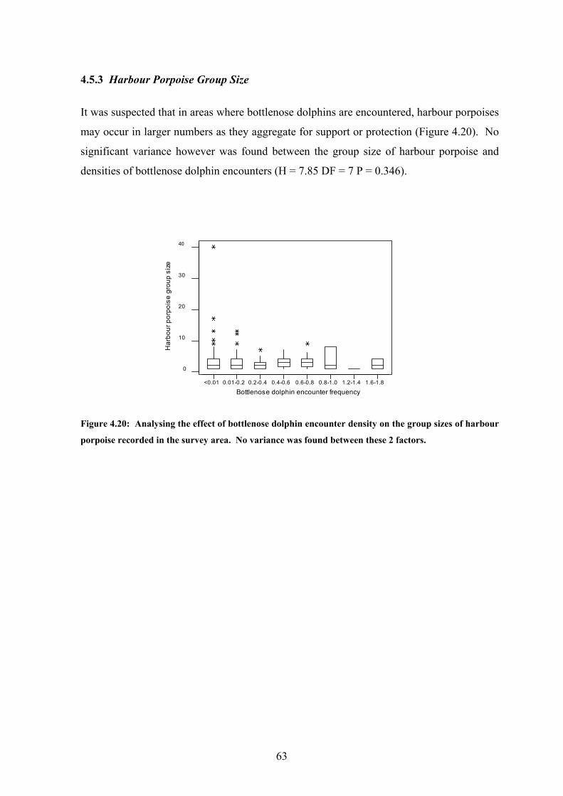
4.5.3 Harbour Porpoise Group Size
It was suspected that in areas where bottlenose dolphins are encountered, harbour porpoises
may occur in larger numbers as they aggregate for support or protection (Figure 4.20). No
significant variance however was found between the group size of harbour porpoise and
densities of bottlenose dolphin encounters (H = 7.85 DF = 7 P = 0.346).
<0.01 0.01-0.2 0.2-0.4 0.4-0.6 0.6-0.8 0.8-1.0 1.2-1.4 1.6-1.8
0
10
20
30
40
Bottlenose dolphin encounter frequency
Har
bour
por
pois
e gr
oup
size
Figure 4.20: Analysing the effect of bottlenose dolphin encounter density on the group sizes of harbour
porpoise recorded in the survey area. No variance was found between these 2 factors.
63

4.6 Results Summary
The results highlighted in the previous section are summarised below:
• The harbour porpoise was encountered in significant numbers in the survey area of
the outer Moray Firth.
• 422 harbour porpoise encounters (1151 individual animals) were recorded during
the survey period of May to October, 2002-2005 inclusive.
• Greater numbers of encounters were recorded with harbour porpoise than any other
cetacean in the other Moray Firth, including the bottlenose dolphin.
• Harbour porpoise sightings were distributed across the survey area from
Lossiemouth in the west to Fraserburgh in the east, and from shallow coastal waters
out to depths of over 100 m.
• Harbour porpoise sightings per unit effort (SPUE) increased with distance from
shore.
• Harbour porpoise encounters declined with increasing sea state.
• A ‘hotspot’ of harbour porpoise encounters was observed in the area of Whitehills.
• All 4 environmental variables; depth, aspect, slope and sediment type showed
significant variance with harbour porpoise encounter frequency.
• Harbour porpoise encounter frequency was only found to be significantly correlated
with depth and slope variables.
• Encounter frequency of the harbour porpoise increased with decreasing depth.
• Encounter frequency of the harbour porpoise increased with increasing slope
gradient.
64

• Regression analysis suggested that the relationship between depth and slope was not
functional and is likely to be influenced by other factors.
• Group sizes of harbour porpoise ranged from 1 to 44 animals. The mean group size
of harbour porpoise was calculated to be 2.9 animals.
• The environmental variables were shown to have very little effect on the group size
of harbour porpoise encounters, with the exception of significant variance, but no
correlation with depth.
• Monthly encounters with harbour porpoise ranged from 1 (May and October 2004)
to 59 encounters (September 2002).
• Encounters followed a significant trend through the survey season with an increase
from May to July, a slight decline in August before peaking again in September. No
monthly trend in distribution was observed.
• Estimated relative abundance was calculated for each year and a dramatic decline
was observed over the 4 year study period. High relative abundance in 2002 and
2003 (0.75 and 0.85 animals / km2 respectively) declined to 0.21 and 0.26 animals /
km2 in 2004 and 2005 respectively.
• No clear trend was seen between number of harbour porpoise encounters and tidal
state.
• Group size increased significantly through May to September during the study
period. No trend was seen between years.
• Bottlenose dolphins were present in significant numbers in the outer Moray Firth
throughout the survey period although numbers varied by survey season from 9 in
2004 to 32 in 2005.
• Bottlenose dolphin encounters were distributed along the entire length of the
coastline but were restricted to coastal wasters with depths of around 20 m.
65

• Harbour porpoise encounters occured in significantly deeper waters than the
bottlenose dolphin.
• Harbour porpoise encounters occurred over significantly different sediment types
than the encounters of the bottlenose dolphin.
• There was no significant difference between the aspect or the gradient of slope
where bottlenose dolphin and harbour porpoise occur.
• Highest encounter densities of bottlenose dolphins were observed in Spey Bay,
Portsoy, Whitehills and Banff.
• Bottlenose dolphin density appears to have a negative influence on the encounter
frequency of harbour porpoise.
• Group size of harbour porpoise was not significantly influenced by the encounter
density of bottlenose dolphins.
66

5. Discussion
67

5 Discussion
5.1 Harbour porpoise distribution With 422 encounters over the 4 seasons, 2002-2005 inclusive, the results from this
study show that harbour porpoises are observed in significant numbers in the waters of
the outer Moray Firth. With the exception of May 2005, encounters with harbour
porpoise were recorded in every month of the 4 survey seasons and were the most
frequently encountered species in the study area overall. Sightings also occurred
throughout the entire survey area, from Lossiemouth in the west to Fraserburgh in the
east, and from the shallow waters close to the coast to the outer limits of the survey area
in depths of greater than 100 m.
It is apparent that the waters of the outer Moray Firth are utilised by harbour porpoise
throughout the entire year with sightings noted throughout the winter season although in
smaller numbers than those reported during the summer (pers.comm. John Smith). The
results from this study indicate that the encounter frequency of harbour porpoise
significantly increases through the summer season from May to a peak in either July or
September depending on the study season. This is consistent with other harbour
porpoise populations such as the results by Gaskin and Watson (1985), who showed
harbour porpoise sightings in New Brunswick, Canada, to peak during the summer
months and Carretta et al. (2001) who noted that the highest densities of porpoise
occurred also during late summer and autumn along the Atlantic coast, in California.
Both studies suggested that seasonal movements are responsible for the variation in
harbour porpoise density throughout the year. Comparable movements have been
observed in other species, including the minke whale, where encounter rates on the west
coast of Scotland were seen to increase again during late summer and autumn, thought
to be due to changes in the shift of or the availability of prey (Macleod et al. 2004).
Peaks in minke whales in the outer Moray Firth have also been noted between July and
September (Tetley 2004) suggesting that the factors influencing the high number of
minke whales may also be responsible for the increase in harbour porpoise numbers in
the area. This idea is further supported by observations of harbour porpoise and minke
whales coexisting in the outer Moray Firth, often encountered feeding in close
proximity to each other (Robinson et al., 2005).
68

It is widely accepted that the distribution of cetaceans is largely governed by the
distribution of their prey (Sheldon et al., 2005; Baumgartner et al., 2000; Davis et al.,
2002; Ruam-Suryan & Harvey, 1998). As highly mobile animals, cetaceans are likely
to remain in an area of high prey density until it becomes more profitable to search for
and move to another (Johnston et al., 2005). In Scottish waters, sandeels constitute
58% by weight of the gross stomach content in harbour porpoise (Santos et al., 1995).
Sandeels are a small schooling fish, of high calorific value which is vital for harbour
porpoise providing a high daily intake of energy necessary to survive (Hislop et al.,
1991). During the winter, sandeels remain in burrows in the seabed until April or May
when the older fish emerge to feed on the plankton in the water column. This coincides
with the start of the increase in harbour porpoise encounters noted in the present study.
Previous studies have highlighted the importance of sandeels in the diet of harbour
porpoise during the summer when the total energy content of sandeels is double what it
was in the spring (Pollack et al., 2000; Hislop et al., 1991). This makes the sandeel
highly profitable as food for harbour porpoise and is likely to encourage harbour
porpoises to areas of high sandeel density. In early autumn, however, gadoids such as
haddock, herring, whiting, pollack and Norway pout have been shown to become more
important in the diet of harbour porpoise, likely to be a result of decreasing numbers or
unavailability of sandeels (Pollack et al., 2000). A further motivation for harbour
porpoise to move into more coastal waters during the spring and early summer might be
to give birth. Shallower, coastal waters, lined with bays and headlands, like that of the
outer Moray Firth, provide valuable sheltered habitats which may attract females ready
to give birth (Lockyer, 1995; Calderan, 2003). The concentration of high calorific prey
in these areas is also vital to lactating females whose consumption demand increases to
80% of its own body weight (Yasui & Gaskin, 1986).
Group sizes of harbour porpoise in general are relatively small in comparison to other
delphinid species inhabiting similar coastal habitats. In the present study, the average
group size of bottlenose dolphin was 13.08 animals (pers.observation), compared to that
of just 2.88 animals in an average group of harbour porpoise. The small group
composition of harbour porpoise has been linked to the acoustics of the species;
Amundin (1991) suggested that the short wavelength, ultrahigh frequency sonar used
for close range navigation and foraging in coastal habitats severely restricted their long-
range whistle development and might be responsible for the limited social organisation
of the species.
69

The group size of the harbour porpoise in the outer Moray Firth was shown to increase
significantly throughout each season from 1.6 animals in May to 3.7 animals in
September inclusive of the 4 seasons. In Welsh waters, harbour porpoise were also
recorded to form large aggregations from July onwards, coinciding with the mating and
breeding season and suggesting large groups allow males and females to congregate to
enhance mating success (Calderan, 2003). A similar pattern could be evident in the
outer Moray Firth where mating is also believed to occur at this time, however, with the
exception of calf observations during the study, there is no evidence to date that the area
is an important calving location (Lockyer, 1995; Sonntag et al., 1999). Group sizes of
minke whales on the west coast of Scotland were also seen to increase throughout the
summer. During the spring and summer months, minke whales were generally recorded
alone or in pairs, whilst during the autumn groups of 2 to 10 animals were seen more
frequently. It is suspected that during the autumnal period, minke whales on the west
coast show a shift in prey species from sandeels to herring (Macleod et al., 2004). This
change in prey species may affect the behaviour and foraging tactics of the animals to
the extent that it is more profitable to feed in larger groups. Wursig & Wursig (1980)
suggested that when feeding in coastal areas, where prey is restricted but predictable, it
is more cost-effective to feed individually or in small groups. However, as prey
becomes more plentiful, co-operative feeding becomes more profitable (Eisfeld, 2003)
implying that increased group size may indicate increase in prey availability.
Alternatively, increases in group size may be due to increased numbers of animals
moving into an area which is also likely to be linked to an increase in prey abundance.
In 2004 Whaley & Robinson calculated a relative abundance of 0.75 harbour porpoise /
km2 in the outer Moray Firth and recommended that the area be nominated as a
potential “safe area” candidate for the species. Relative abundance of harbour porpoise
was estimated for each season of the study that showed a dramatic decline from the
results on which Whaley based his recommendations on. From 0.75 animals / km2 in
2002 the relative abundance increased in 2003 to 0.84 animals/km2, higher than any
area covered by SCANS I (Hammond et al., 1995) and vital evidence that the area is
important in terms of conservation of harbour porpoise in the North Sea. However, a
decline of over 75% in abundance was seen in 2004 (0.21 animals / km2), a value which
has not increased greatly in 2005 (0.26 animals / km2). The reduction in survey effort
during 2004, which reduced the opportunity to encounter harbour porpoise, can only
70

partly explain this decline and the survey effort in 2005 was comparable to the effort of
2002 and 2003 and still showed no significant increase in porpoise abundance. The
relative abundance of 2002 and 2003 confirmed Whaley & Robinson’s results that the
area has the potential to be of great importance to harbour porpoise in this North Sea
location. However, in the last 2 years significant events, linked to their prey and
feeding ecology, have clearly occurred to cause a significant decline.
Patterns in porpoise frequency throughout the season have been clearly linked with the
distribution and abundance of their prey. It is therefore logical that fluctuations in
encounter frequency between seasons are likely to be due to changes in prey abundance
and distribution. Sandeel fishing is a vital component of the North Sea fishing industry
and takes around 750 million tons of sandeels annually (Clover, 2005). It has been
documented that sandeel numbers in the North Sea have declined dramatically to a
population of half the 300 billion needed to sustain the fishery (Clover, 2005). In June
of this year, the European Commission imposed a complete ban on sandeel fishing in
the North Sea due to collapse of stocks (Urquart, 2005). Along with overfishing,
climate change has also been implicated as the cause behind such declines which have
already had a notable effect on the breeding success of the seabirds around the east
coast of the UK (Ellie Owen, pers.comm.). This decline in sandeels coincides with the
increase in haddock found in the stomach contents of harbour porpoise during 2002 and
2003 (Santos et al., 2005). A decline in a primary food source is clearly going to have
an effect on the harbour porpoise population. Such patterns were seen during the 1960s
in the southern North Sea when herring stocks crashed, followed by a recovery in recent
years and with it increases in harbour porpoise numbers (Payne et al., 1986; Santos et
al., 2005). If the density of sandeels in the outer Moray Firth has been greatly reduced,
then the harbour porpoise, which rely on the daily consumption of such prey, are likely
to move to areas of more predictable prey occurrence.
Other threats may have played a partial or full role in the observed decline in harbour
porpoise numbers in the outer Moray Firth. Harbour porpoise are an elusive species
that are highly affected by disturbance from noise and vessel traffic, including whale
and dolphin watching vessels, which have increased in number over the last 4 years
(Tetley, 2004). A significant increase has also been observed in large commercial
fishing vessels along the coastal area of the study region during the last 2 years
(pers.observation). During the summer of 2003, pelagic trawlers began trawling the
71

shallow inshore waters of the outer Moray Firth for squid (pers.observation). The
demersal trawling methods used resulted in the destruction of large proportions of
seabed in areas such as Cullen Bay where divers observed the ‘desert-like plains’ left
after the area had been trawled, wiping out all plant and animal life and leaving nothing
but rubble (Bill Ruck pers.comm.). Such activity would clearly affect the sandeel
which relies on the seabed during a large part of its lifecycle; for hibernation during the
winter months and for protection from predators. Such habitat destruction from
trawling would likely eradicate all sandeel populations present at the time, and the
damage caused might further prevent re-colonisation in such areas for a significant
period of time.
With harbour porpoise distribution severely restricted by the location of its prey source,
it is not surprising that no trends in the location of sightings within the study area were
observed in the present investigation. The uneven distribution of porpoise over months
and years indicates the irregular pattern of prey in the area. In other areas of the UK,
the distribution of harbour porpoise has been highly correlated with the tidal state, with
higher numbers of harbour porpoise sighted on rising or flooding tides, which are
thought to bring in plankton rich waters (Calderan, 2003; Sekiguchi, 1995; Gaskin &
Watson, 1985; Raum-Suryan, 1998). In the outer Moray Firth only a slight increase in
sightings occurred during the rising tides, however, this seems to be explained by an
increase in survey effort by similar proportions.
Observations by Maravelias et al., (2000) have indicated that annual differences in prey
distribution and abundance are not governed by environmental factors such as sea
surface temperature alone, but also by bathymetry and substrate type. Such factors are
therefore likely to provide a valuable insight into the dynamics of habitat choice by prey
species and, as a result, the distribution of predating cetaceans (Maravelias, 1999). The
frequency of harbour porpoise encounters in this study was shown to be influenced
significantly by a number of fixed physical variables in the outer Moray Firth, such as
depth, aspect, slope and sediment type. Depth of the study area ranged from shallow
coastal areas to depths of 250 m within the Southern Trench, located towards the east of
the survey area. The degree of change in depths and slope gradient was seen to be
highly variable across the region. To the west of the study area, changes in depth occur
gradually, reaching only 50 m in depths around 15 km form the shore, in contrast to the
east where depths reached 250 m only 7 km from the coast. The majority of the seabed
72
in the outer Moray Firth faces north. However, in areas of high irregularity, such as the
Southern Trench for example, seabed slopes were observed facing all directions. In
addition, the seabed composed of a number of sediment types. Adjacent to the
coastline, the predominant sediment type is sandy gravel, with gravel and sand present
in Spey Bay. Further offshore, more sand, muddy sand, sandy mud and muddy
substrates are apparent.
With reference to above, using GIS techniques, a significant negative correlation was
found between the encounter frequency of harbour porpoise and with depth. Sightings
increased from the shallow coastal waters up to a mean encounter depth of nearly 36 m.
As depth increased beyond this point, interestingly the sightings were fewer, and this is
consistent with the view that cetaceans in coastal waters as opposed to pelagic waters
are more likely to be influenced by depth (Polacheck, 1987; Baumgartner et al., 2000).
However, that saying harbour porpoise encounters in the outer Moray Firth were
recorded up to depths of 146 m during surveys. Other studies of the species found
similar results. For example, Raum-Suryan & Harvey (1998) noted that porpoise
sightings off the coast of California also occurred at shallow depths and decreased in
frequency with increasing depths. Closer to home, Pollack et al., (2000) found the
distribution of harbour porpoise on the west coast of Scotland to be restricted to depths
less than 200 m.
A number of studies have reported that herring is an important food source for the
harbour porpoise in Scottish waters (Pollack et al., 2000; Evans, 1990), and in
California, Raum-Suryan (1998) noted a positive correlation between the physiographic
features of harbour porpoise and the distribution on herring. Herring is a pelagic fish
noted to be found in greatest abundance in zooplankton rich water depths of 100-150 m
(Maravelias et al., 2000). This information does not comply with the result that the
majority of harbour porpoise in the outer Moray Firth occur in water depths less than 50
m, therefore suggesting that herring may not be as an important food source in this
region. Another possible explanation is that the greater survey effort carried out along
the more coastal route 1 has biased the depth distribution of the harbour porpoise data in
this study. Results from sightings per unit effort calculations clearly indicate this to be
a plausible explanation. Only 0.28 sightings / hour occurred along route 1 while this
value increased considerably with increasing distance from shore up to 0.9 sightings per
hour occurring on the furthest offshore route, number 4. This may correlate with
73

findings by Carretta et al, (2001) in the San Juan Islands, that more porpoise than
expected occurred at depths greater than 100 m.
Research on cetacean habitats around the world has clearly highlighted the importance
of slope gradient in enhancing productivity and it has often been suggested that slope is
the more determining factor governing distribution as opposed to depth (Waring et al.,
2001; Pollack et al., 2000; Sheldon et al., 2005; Gannier et al., 2002). In California,
high densities of harbour porpoise were recorded where deep water canyons intercepted
shallow waters (Carretta et al., 2001), while similar high densities of minke whales in
Scotland were observed in areas of high topographic relief (Macleod et al., 2004). In
this study, harbour porpoise were primarily found on steep slopes of 70˚ to 90˚,
suggesting these areas to be highly productive. In contrast Raum-Suryan & Harvey
(1998) found that harbour porpoise off the San Juan Islands, Washington, were most
often sighted over shallow sloping areas with little topographic relief. Their results
indicated that the gradient of the slope had little effect on the distribution of the prey
species; instead depth was a more influential variable. The differences between the
location of harbour porpoise distribution in this latter study and the outer Moray Firth
could be explained by differences in prey species and their habitat preferences.
Furthermore, aspect was observed to show significant variance with harbour porpoise
frequency, however, it is not thought to directly influence the distribution of the
animals; instead the composition of the slope is thought to be of greater importance as
seen in minke whales in the outer Moray Firth (Tetley, 2004). Therefore, despite the
statistical significance shown by this factor, the biological significance is relatively
minor.
An overwhelming majority of harbour porpoise in the outer Moray Firth were
encountered on sandy gravel sediments; a proportion too great to be explained by
survey bias to these substrates alone. Sandy substrate types are the ideal habitat for the
target sandeel prey (Evans, 1990; Santos et al., 2003). Sandeels spend autumn and
winter in burrows in the sandy sediments before emerging to feed during the spring and
summer in the water column, however the sandeels are restricted to the sandy substrate
throughout the year as it provides a vital shelter from predators (Naud et al., 2003).
Macleod et al., (2004) reported on the correlation between minke whale distribution off
the west coast of Scotland and the sediment type preferred by their prey. In spring
minke whales were found over mainly gravel/sand sediments which are ideal winter
74

settlement grounds for sandeels. In the autumn, however, the distribution of minke
whales altered to more gravel based sediments, highly correlated with herring spawning.
Similar correlations between sandy gravel sediments were noted in minke whale
populations in the St Lawrence Estuary, Canada, and the outer Moray Firth (Naud et al.,
2003; Tetley, 2004). The only variable found to affect the group size of harbour
porpoise was depth, where some variance, but no correlation, was established. Larger
groups were observed between Aberdour Bay and Buckie, close to the coastline
between 20 m and 50 m, which could be due to less predictable or plentiful prey, which
encourages co-operative feeding and an increase in group size from the average group
of 1-3 animals normally encountered (Wursig & Wursig, 1980). Larger groups over
these depths also correlate with the previous theory that porpoises have been observed
to aggregate in these more sheltered waters to breed during the summer (Calderan,
2003). The other topographic variables, however, showed no such pattern.
In summary harbour porpoise in the outer Moray Firth appear to be primarily
concentrated on relatively shallow, steep topographical slopes of sandy gravel sediment.
The sediment types appear to be the most influential factor, in terms of distribution and
habitat selection, due to preferred spawning areas of their prey, whilst the right depth
and slope gradient encourage the settlement of prey on such sediments by enhancing the
occurrence of upwellings and subsequent increases in productivity.
5.2 The influence of bottlenose dolphin on harbour porpoise distribution
Bottlenose dolphins were commonly encountered throughout the survey period of May
to October 2002-2005 inclusive. Sightings of bottlenose dolphins have also been
observed during the winter, although greatly reduced (pers.observation) suggesting a
general trend of bottlenose dolphins moving out of the area during the autumn due to
changes in their prey distribution (Curran et al., 1996). This pattern is consistent with
this study that highlights a peak in dolphin encounters in the month of June followed by
a decline through the following months. These results coincide with the influx of two
important prey species, Atlantic salmon (Salmo salar) and the sea trout (Salmo trutta),
which migrate into the area during late spring and summer returning to their natal rivers
to breed (Mendes et al., 2002; Wilson et al., 1997). As with the harbour porpoise,
encounters of bottlenose dolphin varied with season from only 9 encounters in 2004 to
75
32 in 2005. 2004 also showed a dramatic decline in harbour porpoise sightings
suggesting that the factor causing the decline in porpoise was also responsible for the
decline in dolphins. The increase in fishing activity in 2003 and 2004, discussed
previously, occurred very close to the coastline, causing disturbance and high levels of
noise pollution which would likely have a negative impact on the foraging and social
activity of the coastal cetaceans frequenting this area and may be resulting in them
leaving the area altogether. Significantly fewer trawlers were observed in 2005
(pers.observation), largely due to the ban in sandeel fishery, and without such
disturbance it is to be expected that the animals would return and this is shown by the
significant increase in the number of dolphin sightings. The effect on the harbour
porpoise, however, is more likely to be via their prey source and the destruction of their
habitat which would take considerably longer to recover, and therefore longer for the
numbers of harbour porpoise to return to the area.
The spatial distribution of the bottlenose dolphin in the outer Moray Firth also differs
from that of the harbour porpoise, particularly with respect to depth. Bottlenose
dolphins were almost exclusively found along the 20 m isobath, and never exceeded 30
m. Despite a slight overlap of depths, with harbour porpoise found down to just less
than 7 m, the depths bottlenose dolphins and harbour porpoise occur at is significantly
different, indicating a segregation of the two species. Such species partition involving
bottlenose dolphins has been previously observed in other locations; Atlantic spotted
and bottlenose dolphins were found to differentiate clearly due to depth, with spotted
dolphins found in significantly shallower waters than the bottlenose dolphin. Such
differences were suggested to be due to variations in prey between the two species
(Davis et al., 1998; Hanby, 2003). The results also suggest that bottlenose dolphins are
found in areas of significantly different sediment types to that of harbour porpoise
encounters. Despite both species found most commonly on sandy gravel sediment
types, the bottlenose dolphin was more restricted to sand, gravel and rock sediments
whereas harbour porpoise were encountered in areas of all the sediment types. Along
with encounter depth, the sediment type at sightings is likely to be a consequence of the
feeding ecology of the bottlenose dolphin. The other topographical variables; the
direction and degree of slope showed significant similarity between the two species
with both primarily encountered on steep, northerly facing slopes.
76

The habitat preference of the bottlenose dolphin, like the harbour porpoise and other
cetaceans, is likely to be governed by the distribution of their prey. As already
discussed bottlenose dolphins are found to prey on salmon and sea trout, although other
species may include cod (Gadius morhua), whiting (Merlangus merlangus), saithe
(Pollachius virens) and haddock (Melanogrammus aeglefinus) (Wilson et al., 1997).
The life cycle of the Atlantic salmon and sea trout begins in freshwater rivers before the
long migration to their feeding grounds; which for the salmon are around the Faroe
Islands and off the West Coast of Greenland in the North Atlantic (Bayley & Kindness,
2000). Throughout the summer, the salmon are observed to migrate back to their natal
rivers to spawn (Bayley & Kindness, 2000). Along the coast of the outer Moray Firth,
the River Spey, in Spey Bay, and the River Deveron in Banff are two of the premier
salmon and sea trout Rivers in Scotland. The influx of salmon and sea trout migrating
along the coast to their natal rivers clearly attracts the bottlenose dolphins to the area
and explains the selection of more shallow coastal habitats close to such rivers. The key
role of the migrating salmon and sea trout explains the higher density of dolphin
encounters occurring in Spey Bay and off the coast of Banff. The added attraction to
river mouths is suggested to be due to the fast flowing outflow of waters causing the
fish to be disorientated and making them easier to capture (Mendes et al., 2002).
The recent awareness of the significant threat that bottlenose dolphins impose on
harbour porpoise in the outer Moray Firth has led to the theory that the distribution of
these dolphins are likely to have a significant impact on the distribution of the
porpoises. This was observed in California, where Forney (1995) showed that the
distribution of bottlenose dolphins has shifted north into the study area of central
California, within the range of the harbour porpoise. At the same time, the distribution
of harbour porpoise was noted to move further north and offshore. In recent years,
evidence from sightings and attacks on harbour porpoise has suggested that the
bottlenose dolphin in the Moray Firth have extended their range out of the Moray Firth
and to the south (Stockin & Weir, 2001; Wilson et al., 2004). This study has shown that
in areas of high bottlenose dolphin encounter frequency, the number of harbour
porpoise encounters declines significantly although other factors are also suggested to
be involved such as habitat and climate change. Depth has already been shown to have
a significant impact on porpoise distribution in areas absent of interspecific interactions
with bottlenose dolphins. However, in the outer Moray Firth, it is not possible to
analyse depth and the impact of bottlenose dolphins independently therefore one factor
77

or both simultaneously cannot be shown to govern harbour porpoise distribution in this
area. In the mammalian world, animals have been observed to aggregate into groups as
a form of protection against dangers such as from predation (Treves, 1999). The same
has been observed in cetaceans (McFadden, 2003; Stensland et al., 2003), and in this
respect, harbour porpoises may form larger groups in areas defined as having a higher
encounter frequency with bottlenose dolphins. This theory was rejected, however, as no
significant variance was found between these two factors. In conclusion, the results
from this study clearly indicate that there is some segregation between harbour porpoise
and bottlenose dolphin, in particular with regards to depth. Despite this, the segregation
is not conclusive and a high level of species overlap is observed.
5.3 Limitations
The study of cetaceans is often accompanied by a number of problems and drawbacks
that have to be considered before further work can be carried out and results
implemented. In line transect surveys, it is assumed that g(0) = 1, meaning that all
harbour porpoise along the track line are observed and recorded. In surveys of
cetaceans, however, this is often not the case, as animals can be missed for a number of
reasons, but particularly as cetaceans spend most of their time submerged, thereby
decreasing the chance of being spotted and due to their small size and elusive behaviour
this likelihood is increased in the case of the harbour porpoise. As g(0) decreases from
1, the estimates of occurrence and numbers of harbour porpoise obtained during surveys
become increasingly underestimated. For example, on the west coast of the USA,
Barlow (1988) estimated g(0) to be 0.7690 indicating that just over 23% of all porpoise
were missed. Although it was not possible to calculate a g(0) value for this study,
should Barlow’s estimate be applied to the present findings the relative abundance of
harbour porpoise in the outer Moray Firth would be significantly increased.
Other limitations of the survey are also suggested to enhance the negative bias on the
results. The survey effort was noted to be biased to the coastal route 1 between
Findochty and Rosehearty while the extreme east and west areas of the survey along
with the more offshore survey routes showed reduced effort in terms of distance and
time. Reasons for this variation in survey effort were primarily due to the weather,
which often prevented survey bias conducted further offshore where the sea state was
78
often worse than the coastal route, and time, which often restricted survey trips reaching
the outer limits of the survey area. Such bias must be acknowledged as it has the
potential to affect estimates of abundance and potential trends in populations. This was
noted during the study as the furthest offshore survey route displayed the least effort,
however, the sightings per unit effort showed 0.9 animals / hour to be encountered.
This implies that had the survey effort along this route been as great as that of route 1, a
significantly larger number of harbour porpoise may have been recorded greatly
affecting the relative abundance of the study area. Bias to the coastal route is also likely
to have affected the relationship between harbour porpoise and bottlenose dolphins as
the results would suggest that greater proportions of porpoise were encountered close to
the coast than is actually true, preventing any avoidance on the part of the porpoise
being highlighted.
The sea state during surveys has also been shown to affect the probability of spotting
and accurately observing cetaceans. Harbour porpoise in particular have shown a
decrease in detectability with increasing sea state (Baines et al., 1997; Hammond et al.,
2002; Buckland et al., 2001; Evans 1997). Barlow (1988) observed a large decline in
the detection of harbour porpoise between sea states 2 and 3, while Jones (2004) found
this decrease to occur between sea states 1 and 2. The height of the survey vessel is the
most likely cause for the differences between the two studies as Barlow’s studies took
place from a 10 m platform in contrast to the 3 m platform used in Jones’ survey. In the
present study the vessels used were only just above the water making spotting of
harbour porpoise difficult in sea states greater than 1, explaining the decline in
encounters in sea states greater than this.
The observers themselves during the study clearly imposed limits. The majority of the
observers during the study were volunteers of the Cetacean Research and Rescue Unit,
some of which had never seen cetaceans at sea before. Such inexperience would likely
result in not spotting present cetaceans and inaccurate calculation of group size
(Buckland et al., 2001; Jones, 2004). Measures to reduce this limitation were taken as
at least one staff member with a minimum of two years experience were present at all
times during the surveys.
Finally it should be emphasised that surveys only took place during the summer season
between the months of May and October (September in the case of 2005) and surveys
79
only began and finished part way through May and October respectively. This means
that the trends and estimates discussed during this study only apply to the summer
season and completely different results may occur during the winter season.
5.4 Further research
The limitations of uneven survey effort and inexperienced observers should be
addressed before continuing research in this area. Experienced observers are restricted
as the inexperienced volunteers provided much of the financial backing for the surveys;
however, at least two experienced surveyors should be present during the surveys.
Every effort should be made to ensure even distribution of effort by paying particular
attention to areas of reduced effort.
The distribution of harbour porpoise discussed in this study is clearly correlated with the
life history and habitat of their prey. It is vital therefore when continuing and
expanding research on the habitat and distribution of harbour porpoise that information
regarding their prey is included. Stomach contents of each available stranded animal
should continue to be analysed to build up long term results and patterns in prey choice.
Data from fisheries, such as catch numbers, should also continue to be used as possible
explanations for the fluctuations in harbour porpoise numbers in the area and their
distribution patterns. This further information would enhance our knowledge on the
species and work towards increasing protection of the population. It is essential that
such work is carried out in this area as the results of this study have revealed that the
area has the potential for great importance for the harbour porpoise however numbers
have dramatically declined. Reasons for such a decline need to be understood and
measures put in place to prevent further declines. Other temporal information such as
sea surface temperature, currents, eddies and fronts are also likely to complement this
work on prey distribution.
Further research on the harbour porpoise in the outer Moray Firth should include
acoustics. Incidental sightings of harbour porpoise, suggest that harbour porpoise are
present in the study area throughout the winter season, however, virtually no further
information is known. As surveying is prevented for the majority of the winter due to
lack of funding and bad weather the use of acoustics could provide data on the
80
distribution and population estimates for harbour porpoise utilising this area during
winter. The use of acoustics during the summer would provide a useful additional
research tool, offering answers to questions such as harbour porpoise activity at night
and supplying a more complete data set. T Pods would also provide observer-
independent sightings data and could be used to identify small scale hotspots of harbour
porpoise in the Moray Firth.
Predictive models could be further used to ascertain the probabilities of porpoise
encounters based on physical and environmental variables, the results of which could be
used to find other likely areas of harbour porpoise distribution in other un-surveyed
areas. In comparing different study areas, different factors affecting habitat selection by
harbour porpoise may reveal variations in life history traits amongst different
populations.
81

6. Conclusion
82

6. Conclusion
Harbour porpoise are found in significant numbers and throughout the outer Moray
Firth during the summer season. The encounter frequency and distribution of these
animals are, however, highly variable in terms of time and space. Utilising GIS and
statistical analyses the presence of harbour porpoise was found to be influenced by
physical oceanographic variables such as depth, slope, aspect and sediment type, and
most significantly correlated with depth and slope. The association between these
variables and the encounter frequency of harbour porpoise was due to their influence on
the habitat selection of the primary prey species of the porpoise, the sandeel
(Ammodytes spp.). Seabed of steep slopes, sandy gravel sediments and depths of 30 to
50 m, clearly provided the most ideal, productive habitat for the porpoises. Whilst group
size was not correlated with the physical variables, the time of year had a significant
impact on the number of animals encountered. Larger numbers of harbour porpoise
were encountered later in the season which is most likely related to the life cycle of the
porpoise. During the summer, harbour porpoise were found to move into sheltered
coastal waters to reproduce; aggregations offering protection for new born calves and
enhancing mating success.
The most alarming result shown from this study is the dramatic decline in the annual
relative abundance of the harbour porpoise between 2002 and 2005. During 2002 and
2003, the study area was shown to be an important area for the North Sea harbour
porpoise population, however, less than 25% of the total animals observed in 2003 were
recorded in 2004, and 2005 showed very little sign of recovery. Primary explanations
for the crash in numbers in the outer Moray Firth are disturbance from intensive fishing
in the coastal areas and subsequently the extensive damage to the vital habitat of the
porpoise’s key prey species and effects of climate change. The area clearly has the
potential to be a “safe area”, therefore, it is imperative that the threats and causes of
declines are addressed and rectified immediately in the hope of seeing a return in the
large numbers of harbour porpoise once recorded in the outer Moray Firth.
The recently acknowledged threat to harbour porpoise from interspecific interactions
with bottlenose dolphins has significantly added to the dangers porpoise face in the
Moray Firth. The main group of porpoise affected by these interactions are juveniles of
83

both sexes that are likely to be just starting their reproductive life. With significant
losses within this age bracket, the conservation threat becomes even greater.
Unfortunately for the harbour porpoise this threat is a natural phenomenon that cannot
be reduced through human intervention. With approximately 60% of harbour porpoise
mortality due to interactions with bottlenose dolphins it is vital that all other threats
from fishing, disturbance, pollution and climate change be reduced or ideally
eliminated. The ideal way to accomplish these goals would be to use the results from
this study to improve the management of this species in the Moray Firth, with the aim of
making the area a Marine Protected Area, allowing greater restrictions to be imposed on
activities likely to cause the harbour porpoise harm.
84

7. References
85

7. References ACS online (2005) URL: http//:www.acsonline.org/factpack/harbourporpoise.htm
Adams, J.A (1987) The primary ecological sub-divisions of the North Sea: some
aspects of their plankton communities: In: Development in Fisheries Research in
Scotland. Edited by: Bailey, R.S & B.B. Parish. Fishing News Books, Farnham.
Amundin, M. (1991). Helium effects on the click frequency spectrum of the Harbour
porpoise, Phocoena phocoena. Journal of Acoustic Society of America 90(1):
53-59
Baines, M., C. Pierpoint and S. Earl (1997). A cetacean sightings database for Wales
and an evaluation of impacts on cetaceans from the Sea Empress oil spill.
Report to the Sea Empress Environmental Evaluation Committee. The
Countryside Council for Wales. 70p.
Barlow, J. (1988). Harbour porpoise, Phocoena phocoena, abundance estimation for
California, Oregon, and Washington: I. Ship Surveys. Fishery Bulletin 86(3):
417-432
Baumgartner, M.F. (1997). The distribution of risso’s dolphin (Grampus griseus) with
respect to the physiography of the northern Gulf of Mexico. Marine Mammal
Science 13(4): 614-638
Baumgartner, M.F., K.D. Mullin., L.N. May & T.D. Leming (2000). Cetacean habitats
in the northern Gulf of Mexico. Fishery Bulletin 99:212-239
Bayley, S. & R. Kindness (2000). Management of the Atlantic Salmon in the Marine
Phase, Scotland. A report for the Northern Periphery, 2000.
BBC (18/09 2005) URL: http//:www.bbc.co.uk/news
86

Bjorge, A. & K.A. Tolley (2004) Harbour Porpoise. In: Encyclopedia of Marine
Mammals. Edited by: Perrin, W.F., B. Würsig & J.G.M Thewissen. Academic
Press.
Brodie, P.F. (1995). The Bay of Fundy/Gulf of Maine Harbour porpoise (Phocoena
phocoena): Some considerations regarding species interactions, energetics,
density dependence and bycatch. Paper SC/46/SM3, Report to the International
Whaling Commission (Special Issue 16): 181-187
Buckland, S.T., D.R. Anderson., K.P. burnham., J.L. Laake., D,L. Borchers & L.
Thomas (2001). Introduction to Distance Sampling. Oxford university Press
Calderan, S.V. (2003). Fine scale temporal distribution by harbour porpoise
(Phocoena phocoena) in North Wales: acoustic and visual survey techniques.
M.Sc. thesis. University of Wales, Bangor.
Canadas, A., R. Sagarminaga & S. Garca-Tiscar (2002). Cetacean distribution related
with depth and slope in the Mediterranean waters off Southern Spain. Deep Sea
Research Part I: Oceanographic Research Papers 49(11): 2053-2073
Caretta, J.V., B.L. Taylor & S.J. Chivers (2001). Abundance and depth distribution of
harbour porpoise (Phocoena phocoena) in northern California determined from
a 1995 ship survey. Fisheries. Bulletin. 99: 29-39
Clover, C (2005). Food chain fears may end ‘industrial’ fishing in the North Sea.
Article for the Telegraph.
Croll, D.A., B.R. Tershy., R.P. Hewitt., D.A. Demer., P.C. Fiedler., S.E. Smith., W.
Armstrong., J.M. Popp., T. Kiekhefer., V.R. Lopez., J. Urban & I Gendron
(1998). An integrated approach to the foraging ecology of marine birds and
mammals. Deep Sea Research II 45: 1353-1371
Curran, S., B. Wilson & P.M. Thompson (1996). Recommendations for the sustainable
management of the bottlenose dolphin population in the Moray Firth. Scottish
Natural Heritage Review 56: 74pp
87

Davis, R.W., G.S. Fargion., N. May., T.D Leming., M. Baumgartner., W.E. Evans., L.J.
Hansen & K.D. Mullin (1998). Physical habitat of cetaceans along the
continental slope in the northern central and western Gulf of Mexico. Maine
Mammal Science 14:490-507
Davis, R.W., J.G. Ortega-Ortiz., C.A. Ribic., W.E. Evans., D.C. Briggs., P.H. Ressler.,
R.B. Cady., R.R.Leben., K.D. Mullin & B. Würsig (2002). Cetacean habitat in
the northern oceanic Gulf of Mexico. Deep Sea Research I 49: 121-142
Dunn, D.G., S.G. Barco., D.A. Pabst & W.A. McLellan (2002). Evidence for
infanticide in bottlenose dolphins of the western north Atlantic. Journal of
Wildlife Diseases 38(3): 505-510
Eisfeld, S.M. (2003). The social affiliation and group composition of bottlenose
dolphins (Tursiops truncatus) using the Southern Moray Firth, NE Scotland.
M.Sc. Thesis. University of Wales, Bangor.
Evans, P.G.H. (1990). European cetaceans and seabirds in an oceanographic context.
Lutra 33: 95-125
Evans, P.G.H., C.R. Weir & H.E. Nice (1996). Temporal and spatial distribution of
harbour porpoises in Shetland Waters, 1990-95. European Research on
Cetaceans – 10: Proceedings of the tenth Annual Conference of the European
Cetacean Society, Lisbon, Portugal. pp. 234-237
Evans, P.G.H. (1997). Ecological studies of harbour porpoise in Shetland, North
Scotland. Report to WWF-UK. 106pp.
Fishnet (18/09 2005) URL: http//:www.fishnet.dk
Forney, K.A. (1995) A decline in the abundance of harbour porpoise, Phocoena
phocoena, in nearshore waters off California, 1986-93. Fishery Bulletin 93(4):
741-748
88
Gannier, A., V. Drouot & J.C. Goold (2002). Distribution and relative abundance of
sperm whales in the Mediterranean Sea. Marine Ecology Progress Series 243:
281-293
Gaskin, D.E., G.J.D. Smith., A.P. Watson., W.Y. Yasui and D.B. Yurick (1984).
Reproduction in the porpoises (Phocoenidae): Implications for management.
Report to the International Whaling Commission (Special Issue 6): 135-148
Gaskin, D.E and A.P. Watson (1985). The harbour porpoise, Phocoena phocoena, in
Fish Harbour, New Brunswick, Canada: occupancy, distribution, and
movements. Fishery Bulletin 83(3): 427-442
Hammond, P.S. (1995). Estimating the abundance of marine mammals: a North
Atlantic perspective. In Whales, Seals Fish and Man. Editors Blix, A.S., L.
Walløe and Ø. Ultang. Elsevier Science. pp. 3-12
Hammond, P.S., P. Berggren., H. Benke., D.L. Borcheres., A. Collet., M.P. Heide
Jørgensen., S. Heimlich., A.R. Hiby., M.F. Leopold & N. Øien (2002).
Abundance of harbour porpoise and other cetaceans in the North Sea and
adjacent water. Journal of Applied Ecology 39: 361-376
Hammond, P.S & K. Macleod (2005). SCANS II – estimating cetacean abundance in
European Atlantic Waters. Report by the Sea Mammal Research Unit, Gatty
Marine Laboratory, University of St Andrews.
Hanby, C.L (2003). Relationships of cetaceans to physical oceanographic features.
Journal of Physical Oceanography. 33: 475-575
Harding-Hill, R. (1993). The Moray Firth Review. Scotish Natural Heritage, north-west
region, Scotland. 257pp.
Hislop, J.R.G., M.P. Harris & J.G.M. Smith (1991). Variation in the calorific value and
total energy content of the lesser sand eel (Ammodytes marinus) and other fish
preyed on by seabirds. Journal of Zoology London, 224: 501-517
89

Hui, C.A (1997). Undersea topography and distribution of dolphins of the genus
Delphinus in the Southern California Bight. Journal of Mammology 60: 521-
527
Hui, C.A (1985). Undersea topography and the comparative distributions of two
pelagic cetaceans. Fishery Bulletin 83(3): 472-475
International Fund for Animal Welfare (18/09 2005) URL: http//:www.ifaw.org
Johnston, D.W., A.J. Westgate & A.J. Read (2005). Effects of fine-scale oceanographic
features on the distribution and movements of harbour porpoises Phocoena
phocoena in the Bay of Fundy. Marine Ecology Progress Series 295: 279-293
Jones, N.H. (2004). Abundance and distribution of the harbour porpoise (Phocoena
phocoena) in north Anglesey waters. M.Sc. Thesis. University of Wales,
Bangor.
Kirkwood, J.K., P.M. Bennet., P.D. Jepson., T. Kuiken., V.R. Simpson and J. Baker
(1997). Entanglement in fishing gear and other causes of death in cetaceans
stranded on the coasts of England and Wales. Veterinary Record 141: 94-98
Learmouth, J.A., P.L. Luque., M.B. Santos., I.A.P. Patterson., R.J. Reid., N.J. Spencer
& G.J. Pierce (2005). Mortality and pregnancy rates in harbour porpoise in
Scotland (UK) as estimated from stranded animals. International Commission
for the Exploration of the Sea, Aberdeen 2005.
Lockyer, C (1995). Investigations of aspects of the life history of the harbour porpoise,
Phocoena phocoena, in British Waters. Report of the International Whaling
commission (Special Issue 16): 189-197
Macleod, K., R.Fairbairns., A.Gill., B.Fairbairns., J. Gordon., C. Blair-Myers & E.C.M.
Parsons (2004). Seasonal distribution of minke whales Balaenoptera
acutorostrata in relation to physiography and prey off the Isle of Mull, Scotland.
Marine Ecology Progress Series 277: 263-274
90

Maravelias, C.D., D.G. Reid & G. Swaitzman (2000). Seabed substrate, water depth
and zooplankton as determinants of the pre spawning spatial aggregation of
North Atlantic herring. Marine Ecology Progress Series 195: 249-259
McFadden, C.J. (2003). Behavioural flexibility of feeding dusky dolphins
(Lagenorhynchus obscurus) in Admiralty Bay, New Zealand. M.Sc. Thesis
Texas A & M University in Wildlife & Fisheries Sciences.
Mendes, S., W. Turrell., T. Lütkebohle & P. Thompson (2002). Influence of the tidal
cycle and a tidal intrusion front on the spatio-temporal distribution of coastal
bottlenose dolphins. Marine Ecology Progress Series 239: 221-229
Moore, S.E., D.P. DeMaster & P.K. Dayton (2000). Cetacean Habitat Selection in the
Alaskan Arctic during Summer and Autumn. Arctic 56(1): 132-117
National Geographic (18/09 2005) URL: http//:www.nationalgeographic.com
Naud. M., B. Long., J. Brêthes & R.Sears (2003). Influences of underwater bottom
topography and geomorphology on minke whales (Balaenoptera acutorostrata)
distribution in the Mingan Islands (Canada). Marine Biological Association of
the UK 83: 889-896
Patterson, I.A.P., R.J. Reid., B. Wilson., K. Grellier., H.M. Ross & P.M. Thompson
(1998). Evidence for infanticide in bottlenose dolphins: an explanation for
violent interactions with harbour porpoises? Proceedings of the Royal Society.
London. B 265: 1167-1170
Payne. P.M., J.R. Nichols., L. O’ Brien & K. Powers (1986). The distribution of
humpback whales, Megaptera novaengliae, on Georges Bank & in the Gulf of
Maine in relation to densities of the sandeel, Ammodytes americanus. Fishery
Bulletin 84: 271-277
Pierpoint, C., M. Baines & S. Earl (1998). The harbour porpoise (Phocoena phocoena)
in west Wales. Report to the Joint Marine Partnership of The Wildlife Trusts
and WWF-UK, 28 p.
91
Polacheck, T (1987). Relative abundance, distribution and inter-specific relationship of
cetacean schools in the eastern tropical Pacific. Marine Mammal Science 3(1):
54-77
Pollock, C.M., R. Mavor., C.R. Weir., A. Reid., R.W. White., M.L. Tasker., A. Webb &
J.B Reid (2000). Atlas of cetaceans: distribution in north-west European
Waters. A Report by Joint Nature Conservation Committee.
Raum-Suryan, K.L., and J.T. Harvey (1998). Distribution and abundance of and habitat
use by harbour porpoise, Phocoena phocoena) off the Northern San Juan
Islands, Washington. Fisheries Bulletin 96: 808-822
Reid, G. & J. McManus (1987). Sediment exchanges along the coastal margin of the
Moray Firth, eastern Scotland. Journal of the Geological Society London (A)
144: 179-185
Robinson, K.P., R.M. Culloch., N.J. Duthie., S.M. Eisfeld., M.J. Tetley., J.S. Weare.,
A.R. Whaley & D.J. White (2005). The summer distribution and occurrence of
cetaceans in the coastal waters of the outer southern Moray Firth, NE Scotland.
European Cetacean Conference, La Rochelle, 2005.
Ross, H.M & B. Wilson (1996). Violent interactions between bottlenose dolphins and
harbour porpoise. Proceedings of the Royal Society of. London B 263: 283-286
Santos, M.B & G.J. Pierce (2003). The diet of harbour porpoise (Phocena phocoena) in
the Northeast Atlantic. Oceanography and Marine Biology: an American
Review 41:355-390
Santos, M.B., G.J. Pierce., E.M.Iena., M. Addink., C. Smeenk & C.C. Kinze (2005).
Harbour porpoise (Phocoena phocoena) feeding ecology in the eastern North
Sea. International Commission for the Exploration of the Sea, Aberdeen 2005
92

Sekiguchi, K (1995). Occurrence and behaviour of harbour porpoise (Phocoena
phocoena) at Pajaro Dunes, Monterey Bay, California. Aquatic Mammals 21:
91-103
Shelden, K.E.W., S.E. Moore., J.M.Waite., P.R. Wade & D.J.Rugh (2005). Historic
and current habitat use by North Pacific right whales Eubalaena japonica in the
Bering Sea and Gulf of Alaska. Mammal Review 35(2): 129-155
Sonntag, P.R., H. Benke., A.R. Hilby., R. Lick and D. Adelung (1999). Identification
of the first harbour porpoise (Phocoena phocoena) calving ground in the North
Sea. Journal of Sea Research 41(3): 225-232
Stensland, E., A. Angerbjörn and P. Berggren (2003). Mixed species groups in
mammals. Mammal Review 33(3-4): 205-210
Stockin, K.A and Weir, C (2001). Monitoring the presence and occurrence of
bottlenose dolphins (Tursiops truncatus) in coastal Aberdeenshire waters, North
East Scotland. Report of the Sea Watch Foundation, Oxford. 68pp.
Tetley, M.J (2005). The distribution and habitat preference of the North Atlantic minke
whales (Balaenoptera acutorostrata acutorostrata) in the southern outer Moray
Firth, NE Scotland. M.Sc Thesis. University of Wales, Bangor.
Tillbrook, P.J. (1986). Nature Conservation in the Moray Firth. Proceedings of the
Royal Society of Edinburgh 91B: 13-25
Treves, A (1999). Vigilance and spatial cohesion among blue monkeys. International
Journal of Primatology 70(5): 291-294
Urquhart, F (2005). EC praised for ban on sandeel fishery. Article for the Scotsman.
Weare, J (2003). Abundance and habitat use of harbour porpoise (Phocoena
phocoena) off Point Lynas, Anglesey. M.Sc. Thesis. University of Wales,
Bangor.
93

Whaley, A.R. (2003). The distribution and relative abundance of the harbour porpoise
(Phocoena phocoena L.) in the southern outer Moray Firth, NE Scotland. B.Sc
Thesis, Birkbeck College University of London.
Whitehead, H., S. Brennan & D. Grover (1992). Distribution and behavior of male
sperm whales on the Scotian Shelf, Canada. Canadian Journal of Zoology 70:
912-918
Wilson, D.E., F.R. Cole., J.D. Nichols., R. Rudran and M.S. Foster, editors. (1996).
Measuring and monitoring biological diversity – Standard methods of mammals.
Smithsonian Institution Press, Washington D.C.
Wilson, B., P.M. Thompson & P.S. Hammond (1997). Habitat use by bottlenose
dolphins: seasonal distribution and stratified movement patterns in the Moray
Firth, Scotland. Journal of Applied Ecology 34: 1365-1374
Wilson, B., R.J. Reid., K. Grellier., P.M. Thompson & P.S. Hammond (2004).
Considering the temporal when managing the spatial: a population range
expansion impacts protected areas-based management for bottlenose dolphins.
Animal Conservation 7: 331-338
Wursig, B & M. Wursig (1980). Behavior and ecology of the dusky dolphin,
Lagenorhynchus obscurus, in the South Atlantic. Fishery Bulletin US 77: 871-
890
Yasui, W.Y and D.E. Gaskin (1986). Energy budget of a small cetacean, the Harbour
porpoise, Phocoena phocoena (L.). Ophelia 25(3): 183-197
Yen, P.P.W., W.J. Sydeman & K.D. Hyrenbach (2004). Marine bird and cetacean
associations with bathymetric habitats and shallow-water topographies:
implications for trophic transfer and conservation. Journal of Marine Systems
50: 79-99
94

8. Appendices
95

Appendix 1: Template of the Trip log form used in this study during each boat survey. These forms were laminated and china graph pencils were used to record detailed information about the trip whilst out in the field.
CETACEAN RESEARCH AND RESCUE UNIT
DATE: OBSERVERS : (DD / MM/ YY) (PLEASE CIRCLE) (ADD OT HERS:) START TIME: END TIME: SURVEY: PART / FULL (HH:MM 24 hrs) (HH:MM 24 hrs): (PLEASE CIRCLE) DEPART SEA STATE: 0 1 2 3 4 FROM: (CIRCLE A S AP PROP RIATE: 0-Calm, 1-Ripples, 2-Slight wavelets, 3-Larger waves, 4-Choppy, m any w hite caps )
GPS - DEPARTURE: N (N 00'.00''.000 W 00'.00".000) W ACTUAL ROUTE COVERED: (WHITEHILLS-CROVIE-PENNAN ETC.) ………..…. ………………………………………………………………………………………………………… ……………………………………………………………………………………………………………………… ADDITIONAL INFORMATION / REMINDER : ……………………………………………………..……………………………………………………………………………………………………………………………………………………….. ……………………………………………………..……………………………………………………………………………………………………………………………………………………….. ……………………………………………………..……………………………………………………………………………………………………………………………………………………….. ……………………………………………………..……………………………………………………………………………………………………………………………………………………….. ……………………………………………………..……………………………………………………………………………………………………………………………………………………….. ……………………………………………………..………………………………………………………………………………………………………………………………………………………..
96

Appendix 2: Encounter log used to record sightings of harbour porpoises during boat surveys.
CETACEAN RESEARCH AND RESCUE UNIT
Porpoise Encounter Log
v2.0
Date Time Number of animals GPS Bearing Activity Start End Adults Calves [N 00'.00''.000] [W 000'.00''.000] Direction,
Circling Feeding,Foraging,Travelling
97

Appendix 3: Encounter log used to record sightings of bottlenose dolphins during boat surveys.
CETACEAN RESEARCH AND RESCUE UNIT - Encounter FormEN C OUN TER N O. D ATE: OBSERVERS: (e.g. # 1, # 2 etc.) (D D / M M / YY) ...……………………………………………………………
TIM E STAR T: G PS STAR T: TIM E EN D : G PS EN D : (HH:M M 24 hrs): (N 00'.00''.00 W 000'.00''.00) (HH:M M 24 hrs): (N 00'.00''.00 W 000'.00''.00)
N N
W WG EN ER AL AR EA at STAR T: G . AR EA at EN D :(e.g. Buckie harbour)
LAN D M AR K L.M AR K at EN D :( e.g.100m N W of harbour entrance )
IN D IVID UALS PR ESEN T PHOTO I.D .Structure Film N os. of subgroups: (e.g.KR61 & N D 3 etc)(e.g. 3A (1C) + 6A + 2A)
Activity(PL E ASE T ICK)
FO RA G IN G TRA N SITIN G A G G RESSIO N M ILLIN G H A LF BREA CH IN G SYN CH BREA CH FEED IN G TA IL SLA PS SPY H O PS BO W RID IN G FU LL BREA CH IN G PO RPO ISIN G O TH ER (PLEA SE SPECIFY) O R CO M M EN TS
98

Appendix 4: Hard paper copy used to record harbour porpoise encounters. Data is transferred from the encounter log forms onto these before the data is entered into the computer databases (page 1 or 2).
Cetacean Research & Rescue Unit
Harbour Porpoise Survey Form
DATE: …………………………………… OBS 1:
VESSEL: …………………………………… OBS 2:
ACTUAL ROUTE: ………………………… OBS 3: ………………………………………………… OBS 4:
………………………………………………… OBS 5:
BND / INNER / MID / OUTER (Please Circle) OBS 6
SURVEY START TIME: SURVEY FINISH TIME
NO. OF ENCOUNTERS: TOTAL NO. PORPOISE ENCOUNTERED:
SURVEY / ENCOUNTER NOTES SUMMARY:
………………..................................................................................................................................................................................................................................................................................................................................................................................................................................................................................................................................................................................................................................................................................................................................................................................................................................................................................................................................................................................................................................................................................................................................................................................................................................................................
ENVIRONMENTAL INFORMATION AT SURVEY START:
WEATHER: SUNNY CLOUDY BUT BRIGHT OVERCAST
RAIN FOG
OTHER .............................................................................. SEA STATE (Beaufort
scale e.g. 1-2): .................... TIDES (high, low, rising, falling) SPRING
NEAP SEA HEIGHT (m)……………….
PHOTO ID: YES/NO FILM Nos: ..........................……… FRAMES:
99

SEA STATE
GPS
TOTAL
NO.
ENC No.
(O-4)
TIME
START
TIME END
N 57° 00.000
W 000° 00.000
ADULTS
CALVES
BEARING (e.g. NE)
ACTIVITY
(e.g. travelling, foraging etc)
1
2
3
4
5
6
7
8
9
10
11
12
13
14
15
16
17
18
19
20
100

Appendix 5: Hard paper copy used to record bottlenose dolphin encounters. Data is transferred from the encounter log forms onto these before the data is entered into the computer databases.
Cetacean Research & Rescue Unit Bottlenose Dolphin Survey Form
DATE: ………………………………………. OBS 1: ……………………………………………………
VESSEL: ………………………………….… OBS 2: ……………………………………………………
START TIME: ………………………....…… OBS 3: ………………………………………………..…..
END TIME: …….………………………...… OBS 4:………………………………………………….…
AREAS COVERED:………………………… OBS 5: ……………………….……………………...……
………………………………………………. OBS 6: …………………………………………………...
ENC # …. ENCOUNTER START ………….. ENCOUNTER END: …………… (24 hrs) (24 hrs)
GPS START : N ……………………..……..…….. GPS END : N …………………….……………………
W ………………………………….. W ……………………….…………………
AREA START: …………………………………….. AREA END: …………………….………………………. e.g. Cullen Bay
LANDM ARK START: …………………………………………………………………………………………….. e.g. 100m East of Bow Fiddle Rock
LANDM ARK END: ……….……………………………………………………………………………………….
MAX NO DOLPHINS: .……. [ NO. SUBADULTS: …. TOTAL CALVES: . …. NO. NEONATES:.….]
NO. SUBGROUPS: ....…… SUB-GROUP STRUCTURE (e.g. 3 + 2 + 3+5): .…………………………………
SEA STATE(0-4)……. W ATER T EMP (C)……… ….. DEPTH(M)………….. SPRING NEAP TIDE HEIGHT(m)…
ENCOUNT ER START TIDE (risin g, fallin g, high, low) W EAT HER: SUNNY CLOUDY BUT BRIGHT OVERCAST RAIN FOG OT HER
ACTIVITY:
FORAGING FEEDING TRANSITING MILLING FULL BREACHING SPY HOPS TAIL SLAPS PORPOISING HALF BREACHING BOW RIDING AGGRESSIVE BEHAVIOUR SYNCHRONISED BREACHING OTHER .....................……………….……………………………….
NOTES / SUMMARY :
……………….............................................................................................................................................................
.....................................................................................................................................................................................
.....................................................................................................................................................................................
.....................................................................................................................................................................................
ENVIRONM ENTAL INFORM ATION AT SURVEY START:
WEATHER: SUNNY CLOUDY BUT BRIGHT OVERCAST RAIN FOG
OTHER .............................................................................. SEA STATE (Beaufort scale e.g. 1-2): ....................
TIDES (high, low , r is ing, fa lling) SPRING? NEAP? SEA HEIGHT (m)……………….
PHOTO ID: YES/NO FILM Nos : ..........................……… FRAMES: ................….................. KNOWN INDIVIDUALS PRESENT: .........................……….................................................................................
T r
i p
i
n f
o
101

Appendix 6: CD rom containing raw survey and sightings data of harbour porpoise and bottlenose dolphin encounters collected during the present study.
A CD Rom Should be Attached Here
102