The sovereign debt crisis in Europe:

Lessons from the past, questions for the future

Academic Consultants Meeting

Federal Reserve Board Washington DC

May 6 , 2013

Roberto Perotti IGIER – Bocconi University, CEPR and NBER

Many European countries have high levels of public debt, and are going through periods of budget

austerity. Many economists and policymakers fear that these austerity programs might exacerbate the

recession; others argue that properly designed austerity programs can even be expansionary. This essay is in

two parts. I briefly review what we know about the likely effects of these fiscal consolidations. Then I review

the measures taken so far to cope with the sovereign debt crisis, and the proposals under discussion for

further measures.

Fiscal consolidations: the mean comparison approach

A first method to investigate the effects of a fiscal consolidation is simply to extrapolate from current

estimates of tax and spending multipliers, from time series Vector Autoregression studies. There are several

recent surveys of existing results, mostly based on US data. Therefore, I will concentrate on studies that focus

explicitly on episodes of fiscal consolidations.

Focusing especially on fiscal consolidations introduces a larger cross country set of events; it is also

useful if nonlinearities are important, and the results depend on the size of the initial government debt or

deficit, the size of the fiscal adjustment, or even less easily defined things like the “sense of crisis”.

1

Two statistical approaches have been used to study large fiscal consolidations. The first consists of a

simple comparison of means of variables over time. Specifically: (i) define a “fiscal consolidation”, for instance

as a country-year when the discretionary 1 decline in the primary deficit is more than, say, 1.5 percent of GDP,

or two consecutive country-years when it is at least 1 percent each year; (ii) take a macroeconomic variable of

interest, like private consumption, and compare the average of that variable in the two years after (or during)

the consolidation with the average in the two years before the consolidation. This “mean comparison”

approach would provide unbiased estimates of the average effects of consolidations if the latter were

completely random events (in which case it is essentially a difference – in – difference estimator).

This is the methodology applied by Alesina and Perotti (1995) and Alesina and Ardagna (2010) with

cyclically adjusted data, and by Alesina and Ardagna (2012) with the narrative IMF data of Devries et al.

(2011).2 The typical result is that spending-based consolidations (where the discretionary decline in the

deficit consists of at least 50 percent spending cuts) tend to be longer-lasting and are associated with an

increase in GDP growth or a small recession, while tax-based consolidations are short-lived and are associated

with a slowdown in growth or even a recession. With some variations, all of private consumption, investment,

and exports display this pattern. Also, in general these variables are particularly responsive to cuts in social

spending or spending on public wages and salaries – the two largest government spending items in all OECD

countries.

1 The “discretionary” change in the deficit is that part of the change in the deficit that is not due to the automatic response of the deficit to the economic cycle. In this sense, it can be interpreted as the part of the change in the deficit that is due to intentional actions by the policymakers, like changes in tax rates, in replacement rate for unemployment benefits, in defense spending etc. The same definition applies to each individual budget component. 2 There are two methods to obtain “discretionary” measures of a change in a budget variable. First, the “cyclical adjustment” method: estimate the elasticities of that budget variable to, say, output and inflation, and subtract from the actual change in the budget variable the change in output multiplied by the output elasticity and the change in inflation multiplied by the inflation elasticity. Second, the “narrative” method, pioneered by Romer and Romer (2010) for revenues changes: use budget documents to infer the discretionary change in tax revenues or spending enacted by any law that has consequences for the budget. Devries et al. (2011) compute yearly discretionary changes in government spending and revenues during periods of deficit reductions in 15 countries.

2

Fiscal consolidations are typically multi-year events. In this methodology, a fiscal consolidation lasting

four years would appear as three consecutive two-year consolidations; moreover, a given year can appear in

all of the “pre”, “during” and “post” groups at different dates. It is not clear what the “mean comparison”

method delivers in these cases.

A second problem with this approach is that it is difficult to control for concomitant effects. For

instance, one typical result is that spending-based consolidations are associated with real depreciation of the

exchange rate and improvement in relative unit labor costs. Is this a consequence of spending-based

consolidations, or is this the result of policies typically implemented together with spending based

consolidations? As always, causality is difficult to ascertain.

The accompanying policies might take several forms which might be difficult to capture with one or

two variables: consider for instance labor market reforms, or changes in exchange rate or monetary policy

regimes. Finally, the government budgets and accompanying technical documents need to be studied in

depth in order to determine the discretionary measures with a minimum of confidence.

Fiscal consolidations: case studies

For all these reasons, it is useful to complement the existing evidence with a different approach.

Perotti (2012) presents a detailed discussion of the four largest spending-based consolidations - Denmark

1983-87, Ireland 1987-89, Finland 1992-96, Sweden 1993-97 - based on the original budget documents and on

contemporary discussion, like OECD or IMF annual reports, and country-specific sources.3 I focus on two

questions. First, is there evidence that large budget consolidations can have expansionary effects in the short

run? Second, how useful is the experience of the past as a guide to today’s Eurozone countries?

The main conclusions of the case studies I present are:

3 The pros and cons of case studies vs. an econometric approach are well known. Hence, I will not revisit this debate here.

3

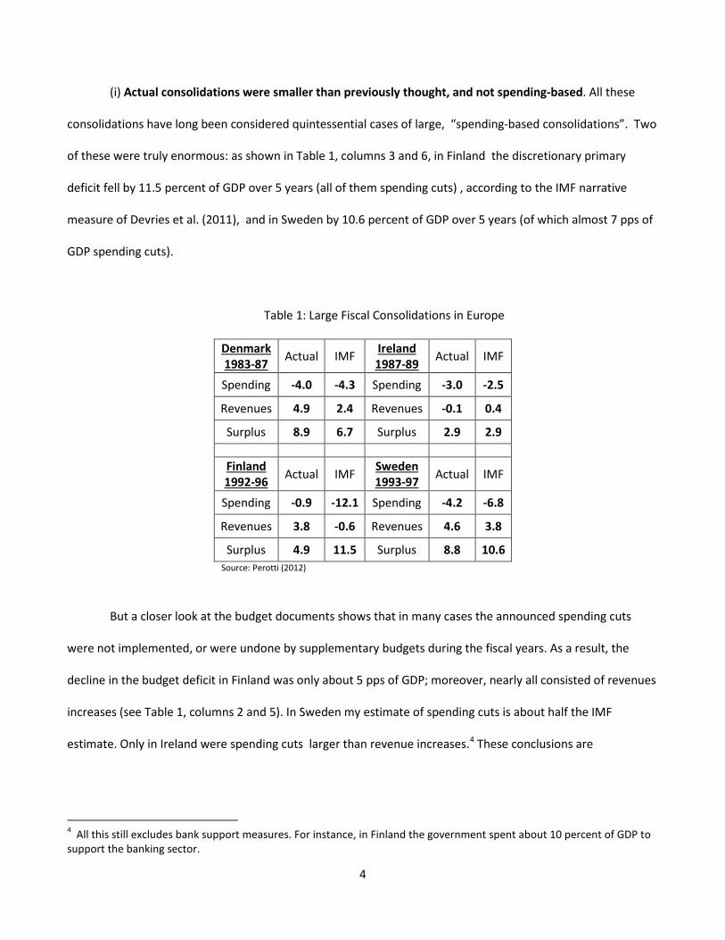
(i) Actual consolidations were smaller than previously thought, and not spending-based. All these

consolidations have long been considered quintessential cases of large, “spending-based consolidations”. Two

of these were truly enormous: as shown in Table 1, columns 3 and 6, in Finland the discretionary primary

deficit fell by 11.5 percent of GDP over 5 years (all of them spending cuts) , according to the IMF narrative

measure of Devries et al. (2011), and in Sweden by 10.6 percent of GDP over 5 years (of which almost 7 pps of

GDP spending cuts).

Table 1: Large Fiscal Consolidations in Europe

Denmark 1983-87 Actual IMF Ireland

1987-89 Actual IMF

Spending -4.0 -4.3 Spending -3.0 -2.5

Revenues 4.9 2.4 Revenues -0.1 0.4

Surplus 8.9 6.7 Surplus 2.9 2.9

Finland 1992-96 Actual IMF Sweden

1993-97 Actual IMF

Spending -0.9 -12.1 Spending -4.2 -6.8

Revenues 3.8 -0.6 Revenues 4.6 3.8

Surplus 4.9 11.5 Surplus 8.8 10.6 Source: Perotti (2012)

But a closer look at the budget documents shows that in many cases the announced spending cuts

were not implemented, or were undone by supplementary budgets during the fiscal years. As a result, the

decline in the budget deficit in Finland was only about 5 pps of GDP; moreover, nearly all consisted of revenues

increases (see Table 1, columns 2 and 5). In Sweden my estimate of spending cuts is about half the IMF

estimate. Only in Ireland were spending cuts larger than revenue increases.4 These conclusions are

4 All this still excludes bank support measures. For instance, in Finland the government spent about 10 percent of GDP to support the banking sector.

4

corroborated by contemporary policy documents and discussions, that do not show any consciousness of living

through a “budget bloodbath”.5

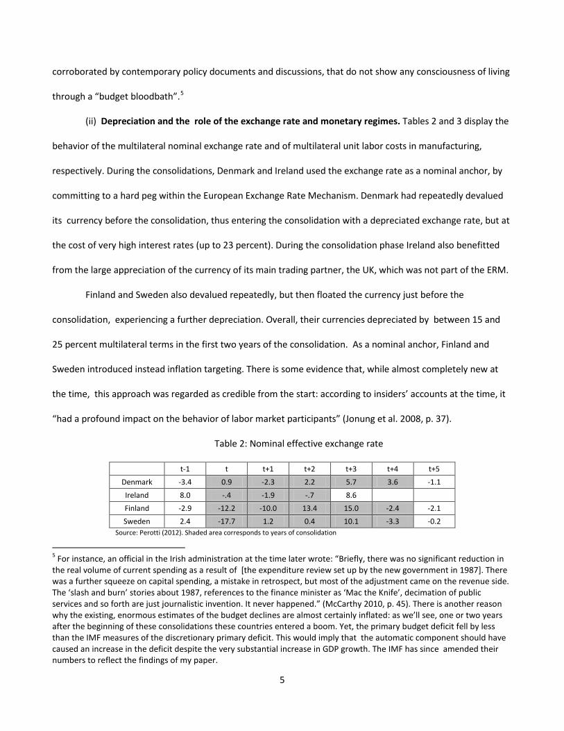
(ii) Depreciation and the role of the exchange rate and monetary regimes. Tables 2 and 3 display the

behavior of the multilateral nominal exchange rate and of multilateral unit labor costs in manufacturing,

respectively. During the consolidations, Denmark and Ireland used the exchange rate as a nominal anchor, by

committing to a hard peg within the European Exchange Rate Mechanism. Denmark had repeatedly devalued

its currency before the consolidation, thus entering the consolidation with a depreciated exchange rate, but at

the cost of very high interest rates (up to 23 percent). During the consolidation phase Ireland also benefitted

from the large appreciation of the currency of its main trading partner, the UK, which was not part of the ERM.

Finland and Sweden also devalued repeatedly, but then floated the currency just before the

consolidation, experiencing a further depreciation. Overall, their currencies depreciated by between 15 and

25 percent multilateral terms in the first two years of the consolidation. As a nominal anchor, Finland and

Sweden introduced instead inflation targeting. There is some evidence that, while almost completely new at

the time, this approach was regarded as credible from the start: according to insiders’ accounts at the time, it

“had a profound impact on the behavior of labor market participants” (Jonung et al. 2008, p. 37).

Table 2: Nominal effective exchange rate

t-1 t t+1 t+2 t+3 t+4 t+5 Denmark -3.4 0.9 -2.3 2.2 5.7 3.6 -1.1

Ireland 8.0 -.4 -1.9 -.7 8.6 Finland -2.9 -12.2 -10.0 13.4 15.0 -2.4 -2.1 Sweden 2.4 -17.7 1.2 0.4 10.1 -3.3 -0.2

Source: Perotti (2012). Shaded area corresponds to years of consolidation

5 For instance, an official in the Irish administration at the time later wrote: “Briefly, there was no significant reduction in the real volume of current spending as a result of [the expenditure review set up by the new government in 1987]. There was a further squeeze on capital spending, a mistake in retrospect, but most of the adjustment came on the revenue side. The ‘slash and burn’ stories about 1987, references to the finance minister as ‘Mac the Knife’, decimation of public services and so forth are just journalistic invention. It never happened.” (McCarthy 2010, p. 45). There is another reason why the existing, enormous estimates of the budget declines are almost certainly inflated: as we’ll see, one or two years after the beginning of these consolidations these countries entered a boom. Yet, the primary budget deficit fell by less than the IMF measures of the discretionary primary deficit. This would imply that the automatic component should have caused an increase in the deficit despite the very substantial increase in GDP growth. The IMF has since amended their numbers to reflect the findings of my paper.

5

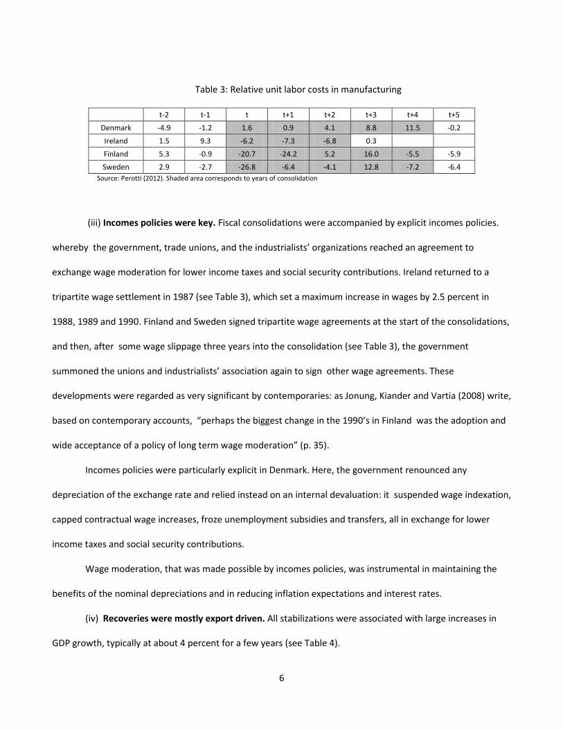
Table 3: Relative unit labor costs in manufacturing

t-2 t-1 t t+1 t+2 t+3 t+4 t+5 Denmark -4.9 -1.2 1.6 0.9 4.1 8.8 11.5 -0.2

Ireland 1.5 9.3 -6.2 -7.3 -6.8 0.3 Finland 5.3 -0.9 -20.7 -24.2 5.2 16.0 -5.5 -5.9 Sweden 2.9 -2.7 -26.8 -6.4 -4.1 12.8 -7.2 -6.4

Source: Perotti (2012). Shaded area corresponds to years of consolidation

(iii) Incomes policies were key. Fiscal consolidations were accompanied by explicit incomes policies.

whereby the government, trade unions, and the industrialists’ organizations reached an agreement to

exchange wage moderation for lower income taxes and social security contributions. Ireland returned to a

tripartite wage settlement in 1987 (see Table 3), which set a maximum increase in wages by 2.5 percent in

1988, 1989 and 1990. Finland and Sweden signed tripartite wage agreements at the start of the consolidations,

and then, after some wage slippage three years into the consolidation (see Table 3), the government

summoned the unions and industrialists’ association again to sign other wage agreements. These

developments were regarded as very significant by contemporaries: as Jonung, Kiander and Vartia (2008) write,

based on contemporary accounts, “perhaps the biggest change in the 1990’s in Finland was the adoption and

wide acceptance of a policy of long term wage moderation” (p. 35).

Incomes policies were particularly explicit in Denmark. Here, the government renounced any

depreciation of the exchange rate and relied instead on an internal devaluation: it suspended wage indexation,

capped contractual wage increases, froze unemployment subsidies and transfers, all in exchange for lower

income taxes and social security contributions.

Wage moderation, that was made possible by incomes policies, was instrumental in maintaining the

benefits of the nominal depreciations and in reducing inflation expectations and interest rates.

(iv) Recoveries were mostly export driven. All stabilizations were associated with large increases in

GDP growth, typically at about 4 percent for a few years (see Table 4).

6

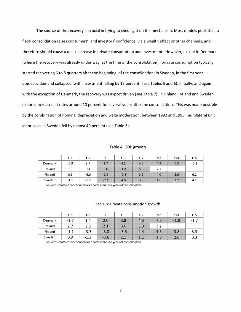
The source of the recovery is crucial in trying to shed light on the mechanism. Most models posit that a

fiscal consolidation raises consumers’ and investors’ confidence, via a wealth effect or other channels, and

therefore should cause a quick increase in private consumption and investment. However, except in Denmark

(where the recovery was already under way at the time of the consolidation), private consumption typically

started recovering 6 to 8 quarters after the beginning of the consolidation; in Sweden, in the first year

domestic demand collapsed, with investment falling by 15 percent (see Tables 5 and 6). Initially, and again

with the exception of Denmark, the recovery was export driven (see Table 7): in Finland, Ireland and Sweden

exports increased at rates around 10 percent for several years after the consolidation. This was made possible

by the combination of nominal depreciation and wage moderation: between 1992 and 1995, multilateral unit

labor costs in Sweden fell by almost 40 percent (see Table 3).

Table 4: GDP growth

t-2 t-1 T t+1 t+2 t+3 t+4 t+5 Denmark -0.9 3.7 2.7 4.2 4.0 4.9 0.3 -0.1

Ireland 1.9 0.4 3.6 3.0 5.6 7.7 Finland 0.5 -6.0 -3.5 -0.8 3.6 4.0 3.6 6.2 Sweden -1.1 -1.2 -2.1 4.0 3.9 1.6 2.7 4.2

Source: Perotti (2012). Shaded area corresponds to years of consolidation

Table 5: Private consumption growth

t-2 t-1 T t+1 t+2 t+3 t+4 t+5 Denmark -1.7 1.4 2.0 3.8 4.3 7.5 -1.9 -1.7 Ireland 2.7 2.8 2.1 3.6 3.3 3.2 Finland -1.1 -3.7 -3.8 -3.5 2.4 4.5 3.8 3.3 Sweden 0.9 -1.3 -3.6 2.1 1.1 1.8 2.8 3.3

Source: Perotti (2012). Shaded area corresponds to years of consolidation

7

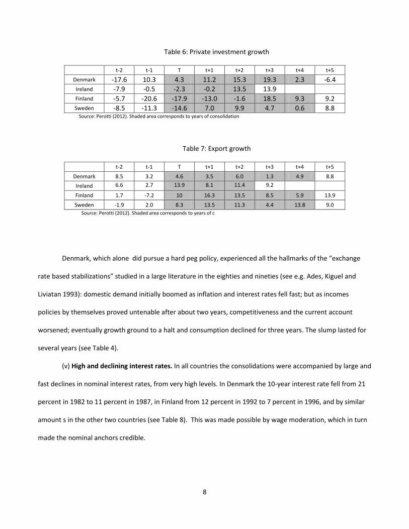
Table 6: Private investment growth

t-2 t-1 T t+1 t+2 t+3 t+4 t+5 Denmark -17.6 10.3 4.3 11.2 15.3 19.3 2.3 -6.4 Ireland -7.9 -0.5 -2.3 -0.2 13.5 13.9 Finland -5.7 -20.6 -17.9 -13.0 -1.6 18.5 9.3 9.2 Sweden -8.5 -11.3 -14.6 7.0 9.9 4.7 0.6 8.8

Source: Perotti (2012). Shaded area corresponds to years of consolidation

Table 7: Export growth

t-2 t-1 T t+1 t+2 t+3 t+4 t+5

Denmark 8.5 3.2 4.6 3.5 6.0 1.3 4.9 8.8 Ireland 6.6 2.7 13.9 8.1 11.4 9.2 Finland 1.7 -7.2 10 16.3 13.5 8.5 5.9 13.9

Sweden -1.9 2.0 8.3 13.5 11.3 4.4 13.8 9.0 Source: Perotti (2012). Shaded area corresponds to years of c

Denmark, which alone did pursue a hard peg policy, experienced all the hallmarks of the “exchange

rate based stabilizations” studied in a large literature in the eighties and nineties (see e.g. Ades, Kiguel and

Liviatan 1993): domestic demand initially boomed as inflation and interest rates fell fast; but as incomes

policies by themselves proved untenable after about two years, competitiveness and the current account

worsened; eventually growth ground to a halt and consumption declined for three years. The slump lasted for

several years (see Table 4).

(v) High and declining interest rates. In all countries the consolidations were accompanied by large and

fast declines in nominal interest rates, from very high levels. In Denmark the 10-year interest rate fell from 21

percent in 1982 to 11 percent in 1987, in Finland from 12 percent in 1992 to 7 percent in 1996, and by similar

amount s in the other two countries (see Table 8). This was made possible by wage moderation, which in turn

made the nominal anchors credible.

8

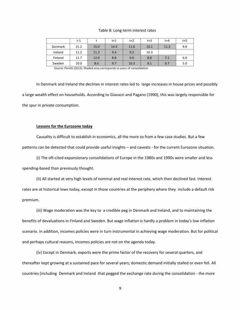
Table 8: Long-term interest rates

t-1 t t+1 t+2 t+3 t+4 t+5

Denmark 21.2 15.0 14.4 11.6 10.1 11.3 9.9

Ireland 11.2 11.3 9.4 9.2 10.3

Finland 11.7 12.0 8.8 9.0 8.8 7.1 6.0 Sweden 10.0 8.6 9.7 10.3 8.1 6.7 5.0

Source: Perotti (2012). Shaded area corresponds to years of consolidation

In Denmark and Ireland the declines in interest rates led to large increases in house prices and possibly

a large wealth effect on households. According to Giavazzi and Pagano (1990), this was largely responsible for

the spur in private consumption.

Lessons for the Eurozone today

Causality is difficult to establish in economics, all the more so from a few case studies. But a few

patterns can be detected that could provide useful insights – and caveats - for the current Eurozone situation.

(i) The oft-cited expansionary consolidations of Europe in the 1980s and 1990s were smaller and less

spending-based than previously thought.

(ii) All started at very high levels of nominal and real interest rate, which then declined fast. Interest

rates are at historical lows today, except in those countries at the periphery where they include a default risk

premium.

(iii) Wage moderation was the key to a credible peg in Denmark and Ireland, and to maintaining the

benefits of devaluations in Finland and Sweden. But wage inflation is hardly a problem in today’s low inflation

scenario. In addition, incomes policies were in turn instrumental in achieving wage moderation. But for political

and perhaps cultural reasons, incomes policies are not on the agenda today.

(iv) Except in Denmark, exports were the prime factor of the recovery for several quarters, and

thereafter kept growing at a sustained pace for several years; domestic demand initially stalled or even fell. All

countries (including Denmark and Ireland that pegged the exchange rate during the consolidation - the more

9

relevant case for today’s Eurozone members) devalued repeatedly before the consolidations. This option is

obviously not available to Eurozone members, except vis-à-vis non-Eurozone members. Ireland also benefitted

from the appreciation of the currency of its main trading partner, the UK. On the other hand, the Danish

expansion was short lived, as it quickly ran into a loss of competitiveness that hampered growth for several

years.

In this paper, I do not want to enter the debate of whether fiscal austerity is needed, how much, and

where. But the observations above suggest that the notion of “expansionary fiscal austerity” in the short run is

probably an illusion: a trade-off does seem to exist between fiscal austerity and short-run growth.

Recent developments and proposals in the sovereign debt crisis

Based on the discussion above, the fiscal consolidations implemented by several European countries

could well aggravate the recession. In this second part I will review the recent measures adopted to cope with

the sovereign debt crisis, and several proposals on the table for further measures.

Obviously, one measure could be to end or split the Eurozone. Many economists and commentators

take it for granted that the Eurozone cannot survive. The reasons why the Eurozone might not be an Optimal

Currency Area are well known. Still, it might be useful to note that, contrary to a widespread impression, the

vast majority of Europeans are in favor of the Euro. In the latest Eurobarometer survey, in all countries except

Cyprus a majority of individuals answered “for it” to the question: “Please state for [the following] proposal

whether you are for it or against it: A European Monetary Union with one single currency, the Euro”. The

percentage of “for it” in Germany was 72 percent, one of the highest. Be as it may, in this paper I do not

intend to take sides on this issue. I will focus on two specific aspects of the measures adopted and of the

proposals on the table.

First, the key feature of the European sovereign debt crisis is the close, two-way interaction between

sovereign risk and financial sector risk. Figure I (at the end of the paper) displays the sovereign and bank CDS

10

premia in selected OECD countries, and their correlation. In most European countries they move closely

together, with correlations of about .5 or above. The correlation in the US is close to 0. The interaction is less

close in the US because, for a variety of reasons, banks hold much less government debt than in Europe.6 In

2012:Q2, Italian and German banks held more than 20 percent of their respective sovereign debt, equivalent to

about twice their capital (see Gros 2013). The first issue I will focus on is to what extent the measures adopted

and proposed address this vicious circle.

Second, it is often argued that the existing problems of the Eurozone stem in large part from the

impossibility of a well-functioning monetary union without a fiscal union. Although this statement seems to

have achieved the status of a “folk’s theorem”, theoretically it is not clear why this should be so. In addition,

the concept of “fiscal union” is rarely spelled out in detail. It typically includes one or more of the following

features: a common deposit insurance, a common unemployment insurance, or a full-fledged federal system

with a Eurozone Economy minister and a large federal budget. In many cases, it seems that two major reasons

for a “fiscal union” are the need for a system of mutual insurance and the need compensate those countries

that experience a loss of competitiveness in the currency union.

Hence one virtually unavoidable feature of all these proposals: in the foreseeable future they would be

asymmetric: they would almost certainly involve large transfers of resources from fiscally healthy countries to

periphery countries. A mutual insurance system under which a set of countries loses in all plausible states of

nature is a political non-starter. It is indeed surprising how a large number of economists and commentators

keep devising ever more sophisticated proposals that would imply an “ex ante” transfer of resources. This

approach is not only not very constructive: it can backfire, by putting unnecessary pressure and blame on the

“donor” countries and possibly inducing them to withdraw from the Eurozone.

6 Among the reasons, aside from moral suasion by the government in at least some countries, is the permanent partial exemption accorded to banks in the EU by article 145 of the Capital Requirements Directive implementing the Basel agreements. It allows European banks that choose internal risk models to apply instead the Standardized Approach (implying zero risk weight) for government bonds (see Gros 2013).

11

In what follows, I will therefore review the main features of the measures adopted so far to cope with

the sovereign debt crisis, and of the main proposal on the table, with a particular focus on the flow of

resources they imply.

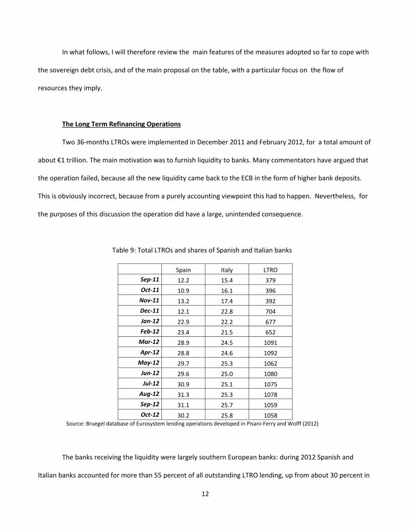
The Long Term Refinancing Operations

Two 36-months LTROs were implemented in December 2011 and February 2012, for a total amount of

about €1 trillion. The main motivation was to furnish liquidity to banks. Many commentators have argued that

the operation failed, because all the new liquidity came back to the ECB in the form of higher bank deposits.

This is obviously incorrect, because from a purely accounting viewpoint this had to happen. Nevertheless, for

the purposes of this discussion the operation did have a large, unintended consequence.

Table 9: Total LTROs and shares of Spanish and Italian banks

Spain Italy LTRO

Sep-11 12.2 15.4 379 Oct-11 10.9 16.1 396

Nov-11 13.2 17.4 392 Dec-11 12.1 22.8 704 Jan-12 22.9 22.2 677 Feb-12 23.4 21.5 652

Mar-12 28.9 24.5 1091 Apr-12 28.8 24.6 1092

May-12 29.7 25.3 1062 Jun-12 29.6 25.0 1080 Jul-12 30.9 25.1 1075

Aug-12 31.3 25.3 1078 Sep-12 31.1 25.7 1059 Oct-12 30.2 25.8 1058

Source: Bruegel database of Eurosystem lending operations developed in Pisani-Ferry and Wolff (2012)

The banks receiving the liquidity were largely southern European banks: during 2012 Spanish and

Italian banks accounted for more than 55 percent of all outstanding LTRO lending, up from about 30 percent in

12

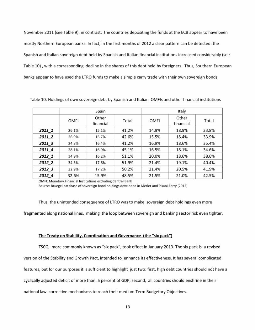
November 2011 (see Table 9); in contrast, the countries depositing the funds at the ECB appear to have been

mostly Northern European banks. In fact, in the first months of 2012 a clear pattern can be detected: the

Spanish and Italian sovereign debt held by Spanish and Italian financial institutions increased considerably (see

Table 10) , with a corresponding decline in the shares of this debt held by foreigners. Thus, Southern European

banks appear to have used the LTRO funds to make a simple carry trade with their own sovereign bonds.

Table 10: Holdings of own sovereign debt by Spanish and Italian OMFIs and other financial institutions

Spain Italy

OMFI Other financial Total OMFI Other

financial Total

2011_1 26.1% 15.1% 41.2% 14.9% 18.9% 33.8% 2011_2 26.9% 15.7% 42.6% 15.5% 18.4% 33.9% 2011_3 24.8% 16.4% 41.2% 16.9% 18.6% 35.4% 2011_4 28.1% 16.9% 45.1% 16.5% 18.1% 34.6% 2012_1 34.9% 16.2% 51.1% 20.0% 18.6% 38.6% 2012_2 34.3% 17.6% 51.9% 21.4% 19.1% 40.4% 2012_3 32.9% 17.2% 50.2% 21.4% 20.5% 41.9% 2012_4 32.6% 15.9% 48.5% 21.5% 21.0% 42.5% OMFI: Monetary Financial Institutions excluding Central Bank Source: Bruegel database of sovereign bond holdings developed in Merler and Pisani-Ferry (2012)

Thus, the unintended consequence of LTRO was to make sovereign debt holdings even more

fragmented along national lines, making the loop between sovereign and banking sector risk even tighter.

The Treaty on Stability, Coordination and Governance (the “six pack”)

TSCG, more commonly known as “six pack”, took effect in January 2013. The six pack is a revised

version of the Stability and Growth Pact, intended to enhance its effectiveness. It has several complicated

features, but for our purposes it is sufficient to highlight just two: first, high debt countries should not have a

cyclically adjusted deficit of more than .5 percent of GDP; second, all countries should enshrine in their

national law corrective mechanisms to reach their medium Term Budgetary Objectives.

13

The six pack is largely a political document, designed to alloy the fears of voters in the core countries. It

is widely regarded as having no real enforcement mechanism, aside from a maximum fine of .1 percent of GDP

that can be decided by the European Court of Justice after a complicated process. Less well known is the fact

that it has an escape clause that can de facto be invoked to nullify its effects: the six pack allows deviations

from targets in the case of unusually low growth, or a European recession. In fact, on April 27 Spain just

obtained a two-year extension on its plan to reach a deficit of 3 percent, citing precisely the unusually low

growth.

Still, the six pack is not entirely without teeth. It has an enforcement mechanism, albeit an indirect

one: if a country that is not in compliance with the six pack cannot have access to emergency funding from the

European funds and from the new bond-buying program of the ECB. I now turn to these important

developments.

The European funds

The European Financial Stability Facility (EFSF, established in June 2010) lends to countries under

specific conditions, by funding itself on the capital market.7 Its debt is backed by guarantees by the Euro Zone

countries, proportional to their shares in the ECB capital. The total guarantees amount to €780bn, which

implies a maximum lending capacity of €440bn (due to an over guarantee of up to 165 percent).8 These are

several guarantees: the maximum amount each guaranteeing country can lose is the face value of its own

guarantee. Currently, the EFSF has committed about €290bn of loans (including up to €100bn for the

recapitalization of Spanish banks).

In October 2012, the new European Stability Mechanism (ESM) became operative; it will overlap with

the EFSF until the latter is phased out completely in 2014. It has a similar lending capacity to the EFSF, €500bn,

7 The EFSF has a small capital of €30bn. 8 This overguarantee is designed to ensure that the entire maximum lending capacity is fully backed by the guarantees of the AAA countries alone, so as to ensure a AAA rating for the EFSF itself. With the recent downgrading of France, the maximum lending capacity has decreased to €293bn.

14

but a different capital structure: €80bn of paid in capital (in five tranches, to be paid up to mid-2014), and

€620bn of callable capital. This difference has often been interpreted as “contrary to the EFSF, the ESM can

leverage up its position”. This is not really correct. Both the callable capital of the ESM and the guarantees of

the EFSF are contingent liabilities of the Eurozone countries; a country can end up losing either the whole

guarantee or the whole callable capital, which are based on the same ECB shares. The key difference is more

subtle, and as far as I know it has gone completely unnoticed. Because of the higher paid-in capital, and other

legal features, including its governance structure, EUROSTAT has decided that the ESM can be considered as

an independent international financial institution; in contrast, the EFSF was considered merely “an accounting

and treasury tool [….] acting exclusively on behalf of” the Eurozone countries (see Eurostat 2011). Hence,

while the debt of the EFSF was allocated pro quota to the gross national debt of each guaranteeing country,

the funds raised by the ESM on the capital market will be considered its own debt, and will not add to the gross

debt of the Eurozone countries. From this point of view, the ESM is politically much more viable for all

countries involved. I believe this is the main reason why the European countries agreed to the change.

To be fair, there are two other differences between the two funds. The EFSF is a pari passu creditor,

while the ESM will have seniority status (after the IMF).9 This change was necessary to make the ESM

acceptable to Germany and the other AAA countries. Seniority is a double-edged sword from the point of view

of moral hazard and the goal of breaking the vicious circle between sovereign debt and financial sector risks.

On one hand, any senior official intervention reduces the private recovery rate on government debt in case of

default. As Gros (2012) shows, the relation between official senior lending and private recovery rate is non-

linear; an initial lending by €100bn reduces the private recovery rate by little, but as official lending as a share

of government debt increases, an additional €100bn of senior lending can reduce the private recovery rate by a

large amount. Hence, an ESM intervention can it concentrate considerable default risk in the portion of

9 It is not clear, however, that the markets really believed that the EFSF would not have been granted de facto seniority.

15

sovereign debt held by the financial sector. On the other hand, it makes the financial sector more cautious

about buying sovereign debt in the future.

The third difference between EFSF and ESM is that the latter will be able to lend directly to the

financial sector, although only once a Eurozone bank supervision system is in place under the ECB. This is in

response to issues raised on the occasion of the EFSF program for the Spanish financial system, that the

Spanish government was reluctant to accept because it was channeled via an agency of its own, thus

increasing the official government debt correspondingly. However, the EFSF loan was pari passu (at least in

theory); an ESM intervention might be channeled directly to the financial system, but will also be senior; thus,

it will not affect directly the private recovery rate of holders of government debt, but will affect the recovery

on banks’ bonds.

Fiscal aspects of the Outright Monetary Transactions program

Whatever its advantages and disadvantages, it is well understood that the ESM will not have enough

resources to address a serious debt crisis affecting Spain and Italy. In the textbook “bad expectational

equilibrium” case, a country suffering from temporary illiquidity might be forced to default because each

would-be lender fears that the others will no longer lend to the country; as a consequence, this expectation

becomes self-fulfilling and the country cannot roll over its debt any longer (see e.g. Calvo 1988).

The textbook solution to such a problem is an announcement that the Central Bank stands ready to

purchase an unlimited amount of government debt. In theory, such an announcement by itself should

eliminate the bad expectational equilibrium, without any actual need of intervention by the Central Bank. On

September 6, 2012, the ECB announced the “Outright Monetary Transactions” program: it stands ready to

purchase and sterilize unspecified but potentially unlimited amounts of government debt on the secondary

market, with maturity up to three years, provided a country were subject to the conditionality of an EFSF/ESM

program.

16

As made clear by the ECB in response to several questions, OMT holdings by the ECB will not have

seniority status. However, there is a subtle issue here. The ECB stated that “it accepts the same (pari passu)

treatment as private or other creditors… in accordance with the terms of such bonds”. Contrary to what most

commentators think, even the holdings of Greek bonds by the ECB, acquired under the (much smaller) OMT

predecessor, the Security Market Program, did not have inherently senior status: “The SMP seniority only

activated when Greece switched the ECB’s holdings into special securities protected from restructuring [….]

That means the ECB could, if hell-bent on avoiding losses through a restructuring, stay legally ‘pari passu’ but

effectively senior anyway “ (Cotterill 2012). As further noted by David Nowakowski of RGE Monitor: “The ECB

can promise to be pari passu, until a default threatens and it can then pressure Euritania to let it swap into

local or international bonds without CACs that receive special treatment, exactly as it did with Greece. They

could still argue, though not in good faith, that those bonds are not senior to anyone, they just got lucky again

to get such a great offer. The ECB has tremendous leverage on countries whose banking systems depend on it

for funding, so it can call the shots.”

In any case, it is widely believed by market participants that the OMT announcement has had a

considerable impact on the spreads of peripheral countries’ debt. But there are two good reasons why

markets might overstate the importance of the OMT program. On the ”demand” side, activation of the

program requires activation of an ESM program; this was designed to obviate the moral hazard problems of

government debt purchases by the ECB.10 But governments are extremely reluctant to enter an ESM program,

which would be perceived as a signal of political failure.

On the “supply” side, it is well known that the German Bundesbank opposed the creation of the

program. Because it is hard to imagine the Eurozone implementing a large program against the opposition of

the Bundesbank, it is of fundamental importance to try and understand the German position. This position has

10 These moral hazard problems were in stark evidence in the summer of 2011 when, just a few days after the ECB announced the purchase of substantial amounts of peripheral debt under the SMP, the Italian government reneged on many budget measures it had previously agreed with the ECB itself.

17

been widely criticized in Europe because it makes little sense in light of the textbook model. To make sense of

it, one must ask what could happen off-equilibrium – always a possibility in the real world. Also, one has to

bear in mind that this program was mostly designed to preempt problems with Spain and Italy, whose

combined stock of government debt approximates €3,000bn. What could happen if the ECB did have to

intervene, buying hundreds of billions worth of this debt? One could envisage at least three problems from a

German point of view.

First, in the real world nobody knows for sure if a country is just illiquid or insolvent. A default by one

or more countries could result in large losses by the ECB. Even disregarding legal technicalities – which seem to

require that national government immediately recapitalize the ECB if it has negative equity - how large a loss

could the ECB sustain? Buiter (2012) estimate about €4,000bn, equal to the present discounted value of all

future seigniorage; Reis (2012) estimates €200bn, obtained with the same method but taking into account a

trend increase in velocity, the incentives of the Central Bank to inflate and the ensuing increase in velocity, and

the currently low interest rates, that imply a very low inflation tax.

Beyond mere economics, the key relevant question is: what is the maximum ECB loss that is politically

sustainable in Germany? For historical and cultural reasons, the answer would have to be: very small. In this

sense, a large OMT intervention would indeed be risky from the point of view of Germany.

Second, is the commitment to total sterilization credible, and would the sterilization be effective

anyway? It is frequently asserted that OMT purchases would be different from QE, because the latter is not

sterilized. Yet the difference appears to be based largely on semantics. The ECB has not stated how it would

sterilize the purchases; a common interpretation is that it would sell equal quantities of government debt of

healthy countries. But it is easy to see that this might not work; the Eurosystem currently holds about €590bn

of government securities; although the ECB does not release the country breakdown, it is likely that most of

this amount consists of debt of problem countries. A large OMT operation on Spanish and Italian debt could

not be sterilized this way. More likely, the ECB would “sterilize” by offering banks to convert their free reserves

18

into 1-week deposits with a minimal remuneration, as it did with the Securities Markets Program launched in

May 2010. However, these deposits are part of the monetary base, and banks would probably regard these

very short term deposits and free reserves as almost perfect substitutes. 11

Third, what happens if, after some time, a country is no longer deemed in compliance with the ESM

program conditions? Realistically, can the stock of debt accumulated by the ECB be liquidated? Also, since

monitoring compliance is entrusted mainly to the Commission, the fear that the process might be influenced

by political considerations (as it has frequently happened in the past regarding compliance with the Maastricht

Treaty and the SGP) is not unfounded. In fact, as we have seen Spain has just been granted an extra two years

to reach its fiscal targets.

“Fiscal union” and Eurobonds

To many in Europe, all these developments should just be preconditions to a “fiscal union”. As

discussed above, the meaning of this expression is rarely spelled out in details, but one component that has

been very frequently advanced in many quarters is a “Eurobond”.

This expression too incorporates a variety of proposals; once again, only in a few cases the details are

spelled out by their proponents. All cite a liquidity premium as a positive effect, which has variously be

quantified from a few basis points to as much as 30 bps. I will not discuss the possible liquidity premium in this

survey, but I will focus on other properties of the main proposals (see Claessens, Mody and Vallée 2012 for a

more complete survey).

The simplest, and for a long time the most common, type of Eurobond proposal is a bond issued at the

central level, which enjoys a joint and several guarantee by each member country.12 In some cases it appears

11 Because of the large MROs and LTROs there is excess liquidity in the system, and this is largely a nominal issue. But in more normal times sterilization would require increasing the interest rate in absorbing operations or issuing longer term debt certificates. 12 In a joint and several guarantee, each guarantor can be called upon to pay for the whole guaranteed amount. That guarantor can then ask the other guarantors to contribute their shares.

19

that each country is supposed to pay for the interest and principal of the share of an issue that it has received;

this would imply no ex ante transfer between countries. But in most cases, it appears that the Eurobonds are

intended to be explicitly a mechanism for ex-ante redistribution, even though exactly how the proceeds of a

Eurobond issue are distributed to and repaid by the individual countries are often not specified. In either case,

the potential for ex-post transfers is significant, via the joint and several liability. But obviously it is unlikely

that a country will be willing to pay the whole amount if other countries refuse to pay their shares, making the

whole construction problematic, if not outright unfeasible.

Indeed, Tirole (2012) shows that a joint and several guarantee cannot be optimal in an asymmetric

environment, in which the guarantor is unlikely to enter distress if the insuree is not in distress. Intuitively, joint

and several liability allows the insuree to borrow more; but to do that, the insuree must be able to compensate

the guarantor. This can happen only if shocks are symmetric, i.e. if the guarantor is equally likely to enter

distress in the future and to be guaranteed by the current insuree.

A proposal that addresses this problem, but only partially, is the so called “Blue and Red Bond”

proposal by Delpla and Weizsäcker (2011). In steady state, an amount of debt up to 60% of the GDP of each

country, called the “Blue bonds”, would be covered by a joint and several guarantee. Any part in excess of

this, the “Red bonds”, can be honored by each country only after the Blue bonds have been honored. And

because the Red debt cannot be guaranteed, bought or rolled over using funds from the ESM, this arrangement

preserves the market signal at the margin. An independent council would decide each year how much Blue

debt a country can issue, based on its performance in terms of some fiscal policy indicators. However, the joint

and several liability can potentially create large transfers between countries, and generate large moral hazard

problems. In addition, in a crisis there would be an enormous political pressure to increase the amount of Blue

debt that a country can issue.

The only Eurobond proposal that avoids the joint and several guarantee is the “European Safe Bonds”

of Brunnermeier at al. (2011). Its specific purpose is to address the vicious circle of sovereign debt and financial

20

sector risks, by providing a large, very safe asset that banks can hold without exposing themselves to

concentrated sovereign risk. The idea is to construct a security by pooling EZ countries’ government debt in

fixed proportions (presumably in proportion to their GDPs) and tranching it in two parts. The junior tranche

absorbs the first X percent of the losses due to a default in any of the underlying government securities. The

senior trance, the ESB, is affected only if the default amounts to more than X percent. By setting X high enough,

the ESB can be made very safe, helping to break at least one part of the link between sovereign debt risk and

financial fragility. To preserve market signals, obviously not all of the debt of each country should be pooled.

One obvious advantage (or disadvantage, depending on the point of view) of the ESB is that it does not

involve any transfer between countries.13 This should make it politically acceptable to the more fiscally healthy

countries. It is also less prone to political manipulation, being based on a simple formula. The problem in

implementing this proposal appears to be of a different nature: “tranching” and “securitization” are not

popular words in the European political and media circles these days. Politicians are reluctant to put forward a

proposal that relies on a widely discredited (if little understood) mechanism.14

Conclusions.

At the time of writing, Eurozone countries seem to have contained the sovereign debt crisis. But they

have done so at the price of strong opposition by German monetary authorities, particularly as concerns the

large government debt purchasing program. I have argued that the main German concerns are not entirely

unfounded, even though they are little debated in policy or academic circles, and that the Eurozone is not likely

to be able to pursue for long a monetary policy that is opposed by Germany.

I have also argued that many proposals for further fiscal “integration” are ill-defined, and in many cases

carry the risk of large permanent transfers that are not politically sustainable.

13 It would involve the possibility of transfers if the safety of the senior tranche were enhanced by a capital cushion paid in by each country, or by a joint and several guarantee. 14 This problem is not purely theoretical: it has indeed arisen in at least one country at the level of discussion with Finance ministry officials (personal communication to the author).

21

References

Ades, A., M. Kiguel, and N. Liviatan (1993): “Exchange-rate-based stabilization: Tales from Europe and Latin America”, World Bank Policy Research Working Paper WPS 1087

Alesina, A. and S. Ardagna (2010): “Large Changes in Fiscal Policy: Taxes versus Spending,” in: Tax Policy and the Economy, Vol. 24, ed. By Jeffrey R. Brown (Cambridge, Massachusetts: National .Bureau of Economic Research)

Alesina, A. and S. Ardagna (2012): “The Design of Fiscal Adjustments”, mimeo, Bocconi University Alesina, A. and R. Perotti (1995): “Fiscal Expansions and Adjustments in OECD Economies”, Economic Policy,

n.21, 207-247. Brunnermeier, M. et al. (2011); “European Safe Bonds (ESBies)”, The Euro-nomics group, September 30, 2011 Calvo, G. (1988): “Servicing the Public debt: The Role of Expectations”, American Economic Review, Vol. 78, No.

4 (Sep., 1988), pp. 647-661 Claessens, S., A. Mody and S. Vallée (2012): “Paths to Eurobonds”, IMF working paper WP/12/172 Committee on the Global Financial System (CGFS) (2011): “ The Impact of sovereign credit risk on bank funding

conditions”, CGFS papers No 43, July 2011 Cotterill, Joseph (2012): “Seniority, the SMP, and the OMT”, FT Alphaville, September 6, 2012

http://ftalphaville.ft.com/2012/09/06/1148941/seniority-the-smp-and-the-omt/ Delpla, J. and j. von Weizsäcker (2011): “The Blue Bond Proposal”, Bruegel Policy Brief, updated version March

2011. Devries, P., J. Guajardo, D. Leigh, and A. Pescatori (2011): “A New Action-Based Dataset of Fiscal

Consolidation,”, IMF Working Paper No. 11/128. Data set available at www.imf.org/external/pubs/cat/longres.aspx?sk=24892.0

Eurostat (2011): “The statistical recording of operations undertaken by the European Financial Stability Facility”, Eurostat news release 13/2011, January 27, 2011

Giavazzi, F and M. Pagano (1990) ”Can Severe Fiscal Contractions Be Expansionary? Tales of Two Small European Countries", NBER Macroeconomics Annual 1990, Volume 5, pages 75-122 National Bureau of Economic Research, Inc.

Gros, D. (2013): “Banking Union with a Sovereign Virus”, CEPS Policy Brief No 289, March 2013 Jonung, L., J. Kiander, and P. Vartia (2008): ”The great financial crisis in Finland and Sweden”, Economic Paper,

DG ECFIN McCarthy, C. (2010): “Ireland’s second round of cuts: a comparison with the last time”, in: Springford, J.:

Dealing with debt: lessons from abroad, CentreForum Canada, Ernst & Young, 41-54 Merler, S. and and J Pisani-Ferry (2012): "Who's afraid of sovereign bonds" , Bruegel Policy Contribution

2012|02, February Perotti R. (2012) "The Austerity Myth: "Growth without Pain?", forthcoming in A. Alesina and F. Giavazzi (eds.)

Fiscal Policy After the Great Recession University of Chicago Press and NBER. Pisani-Ferry, J. and G. Wolff (2012): "Propping up Europe?" , Bruegel Policy Contribution 2012|07, April Romer, C. and D. Romer (2010): “The Macroeconomic Effects of Tax Changes: Estimates Based on a New

Measure of Fiscal Shocks,” American Economic Review, Vol. 100, No. 3, pp. 763-801. Tirole, J. (2012): “Country solidarity, private sector involvement, and the contagion of sovereign crises”,

mimeo, University of Toulouse.

22

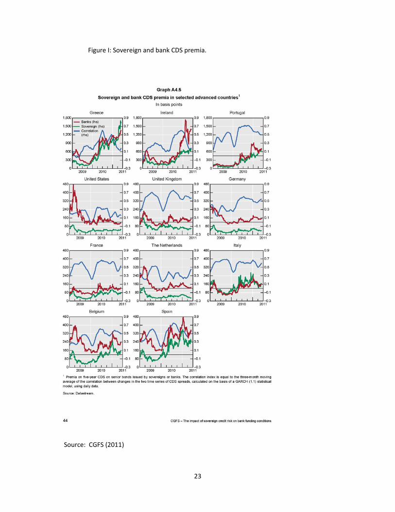
Figure I: Sovereign and bank CDS premia.

Source: CGFS (2011)

23