the slumping of gravity currents

J. Fluid Mech. (1980), voE. 99, part 4, p p . 785-799

Printed in Great Britain 785

The slumping of gravity currents

By HERBERT E. HUPPERT A N D JOHN E. SIMPSON Department of Applied Mathematics and Theoretical Physics,

Silver Street, Cambridge

(Received 25 April 1979 and in revised form 11 January 1980)

Experimental results for the release of a fixed volume of one homogeneous fluid into another of slightly different density are presented, From these results and those obtained by previous experiments, it is argued that the resulting gravity current can pass through three states. There is first a slumping phase, during which the current is retarded by the counterflow in the fluidinto which it is issuing. The current remains in this slumping phase until the depth ratio of current to intruded fluid is reduced to less than about 0,075. This may be followed by a (previously investigated) purely inertial phase, wherein the buoyancy force of the intruding fluid is balanced by the inertial force. Motion in the surrounding fluid plays a negligible role in this phase. There then follows a viscous phase, wherein the buoyancy force is balanced by viscous forces. It is argued and confirmed by experiment that the inertial phase is absent if viscous effects become important before the slumping phase has been completed. R’elation- ships between spreading distance and time for each phase are obtained for all three phases for both two-dimensional and axisymmetric geometries. Some consequences of the retardation of the gravity current during the slumping phase are discussed.

1. Introduction Gravity currents, which result whenever fluid of one density flows horizontally

into fluid of a different density, are frequent occurrences in both natural and man- made situations. Thunderstorm outflows, sea-breeze fronts, estuarine effluences, the discharge of industrial waste water into rivers, lakes or oceans and the sudden release of a foreign gas into the atmosphere are just a few examples. Possibly the most important practical aspect of the study of gravity currents is the determination of the rate of advance of the front. Indeed this is the stated aim of the first theoretical calculation, by von K$rmBn (1940), who purports to prove that a current of density po and depth h propagates under a fluid of density pl( < po) and semi-infinite depth at speed

c = (29’44,

where the reduced gravity g’ = g(po -pl)/pl and g is the acceleration due to gravity. Benjamin ( 1 968) subsequently explained that von KQrmQn’s reasoning in arriving at (1.1) is erroneous but that the same relationship can be obtained by valid arguments. Nevertheless (1 .1) is only a partial solution to the problem: it is but one relationship between the unknown current depth and the unknown current speed.

The determination of the rate of advance of a gravity current arising from the release of a prescribed amount of fluid of density po was first considered by Fay (1 969).

0022-1 120/80/4522-1480 $02.00 0 1980 Cambridge University Press

786 H . E. Huppert and J . E. Simpson

He argues that tthe horizontal buoyancy forces set up by the current are initially balanced by the inertia forces within the current. Fay estimates both these forces and thus evaluates the axisymmetric spreading of a gravity current of fixed volume Q

(1.2) as initially given by

R N (g'Q)it*,

where R is the radial co-ordinate of the front, or nose, of the current. This relationship, argues Fay, is valid until the gravity current becomes so thin that viscous forces, rather than inertia forces, balance the buoyancy forces. Using an order of magnitude evaluation of the viscous force for a current propagating under a free surface, Fay determines that

R N (g'Q2d)&ta,

where v is the kinematic viscosity. By equating (1.2) and (1.3)) Fay argues that an inertia-buoyancy balance is operative if 0 < t c t, and a viscous-buoyancy balance if t , < t, where

Since Fay is primarily concerned with the spread of oil over water, he then in- vestigates a third stage of the spreading, when there is a balance between viscous forces and surface tension.

In a following paper, Hoult (1972) places the above results on a firmer foundation by actually solving governing equations rather than balancing forces. Arguing that the length scale of horizontal variations along the current greatly exceeds the thickness, Hoult bases his analysis on the depth-averaged, shallow-water equations. Entirely neglecting the motion in the upper fluid, Hoult writes down the equations of conservation of mass and momentum in the gravity current. Retaining only the buoyancy and inertia terms, he commences the solution of the equations in terms of the similarity variable

7 = (g'Q)-irt-t for axisymmetric spreading ( 1 . 5 ~ )

= (g'q)-+ xt-8 for two-dimensional spreading, (1.5b)

where q is the volume per unit span. However, conservation of mass and momentum are not sufficient to obtain a complete solution. As argued previously by others (Fannelop & Waldman 1971) an extra conditicn, such as one applied near the front of the current and thus implying that the current is controlled by the head, is seen to be required. The results of Benjamin and experience gained from hydraulic con- trols suggest that the appropriate condition is the specification of the Froude number, Fr = c/(g'h)*, just behind the head. This Froude number should be 24 according to Benjamin, but Hoult suggests expressing it as a constant A*, to be determined from experiment. From a series of two-dimensional experiments of oil spreading over water, Hoult concludes that the best fit to the results comes from h = 1.40. He thus obtains (after we have corrected an algebraic error)

(1.3)

t* = (Q/d)*- (1.4)

R = 1*3(g'&)*t* ( 1 . 6 ~ )

and I = l*G(g'q)it%, (1.6b)

as the spreading laws in the inertia-buoyancy range for the axisymmetric and two- dimensional situations, where 1 is the length of the (two-dimensional) current. Being the results of a similarity calculation, these relationships are expected to be valid only

The slumping of gravity currents 787

after sufficient time has elapsed since the release of the intruding fluid for the initial geometry to be irrelevant.

To evaluate the spreading laws when viscosity dominates inertia, Hoult retains the viscous terms and neglects the inertial terms in the equations for the current and uses the (inertial) boundary-layer equations to describe the motion in the intruded fluid. The analysis then continues via the similarity variable

7 = [~/g'~Q~]l%rt-* for axisymmetric spreading, ( 1 . 7 ~ )

= [~/g'~q~]*xt-Q for two-dimensional spreading. ( 1 . 7 b )

The condition a t the head is now somewhat unsatisfactory since the flow ahead of the current needed to close the problem cannot be of the postulated boundary-layer type: horizontal gradients are not sniall compared to vertical gradients there. Be that as it may, Hoult obtains (after correcting for another algebraic error)

R = 0.94(g'2Q4/~)hta ( 1 . 8 ~ )

and 1 = 1*5(g'2q4/v)W (1.8b)

as the spreading laws valid in the viscous-buoyancy stage for axisymmetric and two- dimensional spreading, where the multiplicative constant 1.5 is determined by experiment and the value of 0.94 follows from it. Like Fay, Hoult continues by considering surface-tension effects.

Prior to the work of Fay and Hoult, a comprehensive series of two-dimensional experiments had been performed by Keulegan (1957). Using a full-depth lock gate, he releasedfixed volumes of salty water, of specific gravities ranging between 1-005 and 1.2 1, into fresh water in channels. Amongst other results, Keulegan reports numerous data of velocity of the front of the resulting gravity current as a function of distance. Differentiating ( l . 6 b ) with respect to time and eliminating t in favour of 1 from the resulting expression by use of (1 .6 b ) itself, we obtain the relationship

u = 1*3(g'q)*Z-*, (1.9)

with which Keulegan's results can be compared. There is little agreement, either quantitative or qualitative, as will be discussed further in 3 3. The only possible con- clusion is that in Keulegan's experiments a different physical process from the ones described above was operative and must be included if the experiments are to be understood.

The aim of the present paper is to point out the extra physics involved and to present a very simple theoretical model incorporating this physics. Keulegan's results are shown t o agree well with our spreading relationships, as do results from additional experiments carried out by us to test the ideas further.

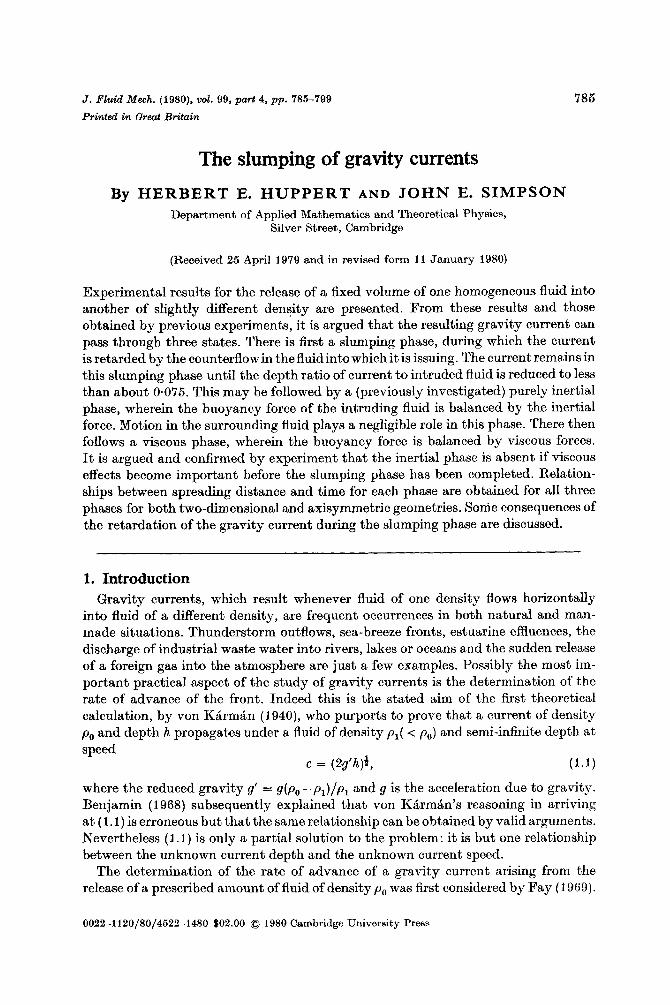
The key point is that the motion of the fluid surrounding the gravity current is dependent upon the fractional depth of the current 4 = h / H , where H is the depth of the surrounding fluid. We show that, until 4 becomes sufficiently small, this motion causes the current to propagate less rapidly than implied by (1.6). The influence of fractional depth on a gravity current of infinite horizontal extent has been discussed theoretically by Benjamin and the influence on the Froude number condition a t the head investigated experimentally by Simpson & Britter (1979) a5 indicated in figure 1. Using these results and a simple model for the shape of a gravity current, we

788 H.E. Huppert and J . E. Simpson

0.0 1 0.05 0.1 0.5 1 .o

FIGURE 1. The Froude number at the head of a gravity current as a function of the fractional depth: x , experimental results from Simpson & Britter (1979) and from this paper; -, (2.1), the analytic relationship used in this paper; ..., the theoretical expression obtained by Benjamin (1968).

hlH

obtain (2.6) and (2 .12) as the speading relationships in what we call the slumping stage, that is the stage in which the dense fluid slumps and fractional depth effects are important. An inertia-buoyancy stage may then follow, as outlined by (1.6) or, as typified by Keulegan’s experiments, viscous effects may overcome inertial effects. The inertia-buoyancy stage as described by Fay and Hoult is then entirely absent.

The model does not attempt to describe the flows in exact detail. In particular, the initial motion, during which the head of the current rapidly accelerates from rest to achieve the speed predicted by the model, is not included. Nevertheless, the model incorporates the major physical principles involved and its predictions agree well with the experimental data.

Gravity currents propagating with large fractional depths occur frequently. For example, sea-breeze fronts often propagate under an atmospheric inversion, which acts as an effective lid and hence produces fractional depths of order & (Simpson, Miiford & Mansfield 1977). Sewage and pollutants are commonly pushed out by man into relatively shallow layers of fluid. A final example comes from mining practice, where explosive gas such as methane can escape and travel along the roof of a mine roadway and endanger life.

2. Theoretical concepts (a) Two-dimensional gravity currents

A simple model, which can be used as a basis of comparison with Keulegan’s experimental results and our own to be presented in 9 3, is based on two assumptions. First, that the slumping takes place through a series of equal-area rectangles (see figures 9 and 10, plates 1 and 2, and the discussion in 9 4). Second, that the Froude number at the head is given by Fr = $#-+ (0.075 6 # < 1)) (2.1)

p r = 1-19 ($ 6 0-075), (2.2) when the gravity current is propagating over a solid surface. The relationships (2.1) and (2.2) based on the results from steady-state experiments reported by Simpson


& BritteF (1979)and from a few additional ones carried out by the present authors, is shown in figure 1. Also shown in figure 1 is Benjamin’s theoretical relationship obtained by modelling the dissipation a t the gravity current interface by a loss of pressure head. Of course, we do not wish to claim that there is a discontinuityin the derivative of Fr against q5 a t q5 = 0.075. We wish merely to model the fact that the variation of Pr with q5 for q5 less than 0.075 is very much less than that for 4 greater than 0.075. The use of ( 2 . 1 ) leads to results in good agreement with the slumping stage, and use of (2 .2 ) with the inertia-buoyancy stage (if this occurs). As seen from figure 1, the relationship (2 .1 ) involves an extrapolation of the data between q5 = 0.075 and qi = 0.3 to beyond q5 = 0.3 , the largest value of q5 for which data can be obtained from steady-state gravity current experiments. The major justifications of using this particular extrapolation are its simplicity and that it leads to predictions in good agreement with the experiments of ourselves and Keulegan.

The first assumption, that of equal areas, implies that

h l = q = h,l,, (2 .3 )

where h, is the depth of the current before the release and I , is its length. Substituting (2 .3) into (2.1) and ( 2 . 2 ) , we obtain

Fr = l*i/(g‘q)* = &(q/lH)-* (0.075 < q/ZH < 1) ( 2 . 4 ~ )

= 1-19 (q/lH < 0.075). (2 .4b )

Integrating ( 2 . 4 ~ ) using the initial condition

1 = 1, ( t = O), (2.5)

we obtain I = [1i+&(g’3qH2)Jt]$ ( I , < 1 < Z, p/0*075H) (2 .6 )

(2 .7 ) = [Z, + g(g’3qH2/z0)* t ] [I + O(g’3qH2t6/1;)+],

where the slumping length 1, is the length of the gravity current when the fractional depth has been reduced to 0.075. Integrating (2 .4b ) using the initial condition

1 = 1, [ t = t, = y(zt - Zi)/(q’3qH2)6], (2.8)

where the slumping time t, is evaluated by setting 1 = 1, in (2 .6 ) , we obtain

I = [@+ 1*78(g’p)*(t-t,)]3 ( I , < I < I * ) (2 .9 )

- 1*47(g’q)ftf (t > t ,), (2.10)

where 1, = ( ~ ~ g ‘ v - ~ ) + is the length scale of the current when the viscous force first exceeds the inertia force, as derived by balancing (1 .6b ) and (2 .10) .

We note that ( 2 . 7 ) indicates that our model predicts that for some time after its initiation the rate of advance of a gravity current of fractional depth greater than 0.075 is a constant [and does not go like t-* as inferred from the inertia-buoyancy balance, cf. (1.6 b ) ] . Further, as is shown in figure 2 and discussed further in the next section, the subsequent evolution of the current as predicted by (2 .6 ) does not depart much from the linear relationship ( 2 . 7 ) . The existence of this approximately constant- velocity regime is well documented by our experiments and those of Reulegan (1957), as is shown in figure 5 to be considered further below. For larger times, the comparison of (2 .10 ) obtained by the simple arguments outlined above, with (1 .6b ) obtained by

790 H . E . Huppert and J . E . Simpson

solving the governing equations of motion and evaluating the multiplicative constant by experiment, is encouraging. It points to the underlying strength of dimensional analysis in simple models !

( b ) Axisymmetric gravity currents

The same two assumptions used in the model of two-dimensional gravity currents can be used when considering axisymmetric currents. The equal-area assumption leads to

nhR2 = Q = Tho R;, (2 .11)

where R, is the initial radius of the current before release. The Froude-number relationships (2 .1 ) and (2 .2 ) are unaltered: on the length scale of the head an axisymmetric gravity current is locally two-dimensional.

Proceeding as for the two-dimensional situation, we obtain the following relationships for a radial current propagating over a rigid surface

R = [ R ~ + + n - ~ ( g ‘ 3 & H 2 ) * t ] ~ [R, < R < rs = (Q/0*075nH)f] (2 .12)

= [R, + + ~ - * ( g ’ ~ & H ~ / R i ) * t ] [ 1 + O(g’3&H2t6/R:)3], (2.13)

and R = [rf+2.37na(g’Q)*(t-t t ,)]* (r, < R < r * ) (2 .14)

- 1.16(gf&)*t* ( t $= ts ) , (2.15)

where r, and r* are the radial equivalents of 1, and 1 *. We note again that for small times the rate of advance is a constant, and remains

approximately so throughout the slumping regime. The agreement between ( 1 . 6 ~ ) and (2.15) is seen to be satisfactory, though it should be recalled that Hoult’s experiments leading to ( 1 . 6 ~ ) were for a gravity current propagating over a free surface and that we are considering a gravity current propagating over a rigid surface. This will be discussed further in 8 4 .

( c ) The viscous-buoyancy phase

In our experiments, and those of Keulegan, the current propagates over a solid boundary and the relationships derived by Fay and Hoult (for propagation under a free surface) are not valid when viscosity is important. The dominant viscous retarding force on the current is then the stress at the solid boundary, ‘rather than. that a t the interface between the current and the adjacent fluid. The continuity and momentum equations for a thin, two-dimensional gravity current of depth h(x , t ) can then be approximated by

h, + (uh), = 0, (2 .16)

g’hh,+ v u / h = 0, (2.17)

where u ( x , t ) is the vertically averaged horizontal velocity and vu/h is the viscous stress per unit mass exerted on the current. Eliminating u from (2.16) and (2 .17) , we obtain

vh,-g’(h3h,), = 0. (2.18)

Together with the volume conservation equation,

(2.19)


No.

1 2 3 4 5 6 7 8 9

10 11 12 13 14 15 16 17 18

14.9 14,9 1.00 14.9 14.9 1.00 14.9 14.9 1.00 15.0 30.0 0.50 15.1 30.0 0.50 14.9 30.0 0.50 15.0 44.0 0.34 14.9 45.2 0.33 15.0 44.9 0.33 15.2 45.0 0.34 14.9 14.9 1.00 7.5 7.5 1.00

29.8 29.8 1.00 5.7 44.4 0.13 5.7 44.6 0.13

10.2 44.2 0.23 7.3 7.3 1.00

11.2 44.3 0.25

39.0 39.6 39.4 39.3 39.3 39.7 39.1 39.3 39.2

118.7 118.2 79.0 20.2 82.5 39.1 40.1 39.0 39.3

581 590 587 589 593 592 587 586 588

1800 1760 593 602 47 0 223 409 285 440

9.1 28-7 54.6 9.4

28.7 61.5

9.4 27.4 64.8 28.1 29.5 11.2 11.2 47.1 87.6 79-0 13.6 44.7

520 528 525 262 264 263 178 173 175 535

1576 1053 269 141 67

123 520 132

112 64.1 46.2 36.7 21.2 14.4 19.1 10.7 7-1

32.9 189 289

37.1 3.8 1.3 4.0

6.0 131

482 574 627 489 571 64 1 481 567 643

1271 1258 503 509 524 336 511 307 496

TABLE 1. The parameters of the 18 two-dimensional experiments.

145.3 105.6 87.7

145.2 106.0 85.1

144.8 106.7 83.6

201.4 195.8 138.7 139.9 80.6 44.0 64-2 86-3 78.8

(2.18) suggests the similarity solution

‘I = [v/(g’q3)]txt-t .

(2.20)

(2.21)

Substituting (2 .20) and (2 .21) into (2 .18) , taking the first integral of the result and evaluating the single constant of integration by using (2 .19) , we determine that

1 = 1*41g’q3/v. (2.22)

A similarity solution for the fluid above the current can be obtained, in a manner analogous to Hoult (1972), but we do not need the results and will hence not present them here. We note, however, that (2 .22) contains no parameters which need experimental evaluation, in contrast to the case of a current propagating under a free surface.

Repeating the above calculations for an axisymmetric current in the viscous- buoyancy phase, we obtain

again without the necessity of experimental evaluation of any constants.

R = 0.894(g’Q3/~)4 t* , (2 .23)

3. Experimental confirmation (a) Two-dimensional

The first series of our experiments was carried out in a Plexiglas channel 9.6m long, 27 em wide and 50 cm high. The channel was very kindly loaned to us by Professor M. S. Longuet-Higgins, FRS. A series of 18 experiments were carried out. The channel was filled with tap water to a depth h, and then a wooden gate was placed


800 - (a)

700 -

600

- 500

- 400

-

- E, c

-

0 20 40 60 80 100 120 140 160

8oo

700

- ( b )

-

600 -

t * ( X ) t* (0)

II 1 I I I I I I I I 0 20 40 60 80 100 120 140 160

t (9 FIGURE 2 . The length of the gravity current as a function of time for four two-dimensional experiments. (a ) x , experiment number 1 ; @ experiment number 2, ( b ) x , experiment number 9; @, experiment number 7. The solid curves ar0 (2.6) and (2.9).

in the channel a t a distance I , from one end. Household salt was added to the water behind the gate until a suitable density was obtained. Further tap water was then added to both sides of the gate, if required, until the total depth of both sides was H . The gate was then quickly removed entirely from the system and the position of the front of the gravity current recorded a t pre-set time intervals.? The parameters of each experiment are given in table 1. Within reason, we tried to encompass as wide a range of initial conditions as possible. In particular, experiments 14 and 15 were

or another and we should like to thank them collectively here. t Almost every fluid dynamicist in D.A.M.T.P. was involved in the timing of one experiment


A +

a A A

0.1 0.5 1 5 10 0.0 I 0.05 0.1

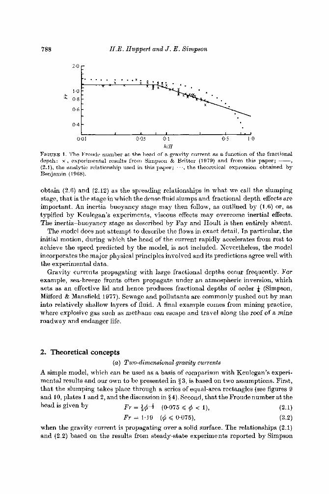
tlt, FIGURE 3. The ratio of the measured length of the 18 two-dimensional gravity currents to the

predicted length in the slumping phase as a function of t / ts.

0.1 I I I I I I I I 1 I I l l I 0.0 1 0.05 0.1 0.5 1 5 10

tlt.

FIGURE 4. The ratio of the measured length of the 18 two-dimensional gravity currents to (g'q)f t8 as a function of t/t,. The straight line included in the figure is (2.22), the relationship suggested for t $ t* if no mixing takes place.

performed with small initial fractional depths to confirm that the simple buoyancy- inertial relationship (1.6 b ) could be attained in our experimental configuration.

Figure 2 presents the length of the gravity current during the early stages of four experiments and compares them .with the prediction of (2.6) and (2.9). The agreement is seen to be good for t less than approximately 0.5t, E 0.5(q4/v3g'2)3. Beyond this

794 H . E. Huppert and J . E. Simpson

h

w 2 5 1

3 20 X

X

0

0 0

I 1 I I I I I I J

0 250 500 750 1000 1250 1500 1750 2000

1 (cm)

I I I I I I I I I

I (cm)

0 250 500 750 1000 1250 1500 1750 2000

FIGURE 5. Keulegan's memured velocity of the nose of a two-dimensional gravity current as a function of its length. The solid curves, drawn for 1 > I", are our prediction, (3.2). (a ) X ,

h, = H = 26.0cm, 1, = 188.0cm, g' = 191-7 cm 8-2, r* = 3409 cm; @, h, = H = 11*6cm, I , = 83.5 cm, g' = 59.6 cm s-2, z* = 908 cm. 1, = 188.0 cm, 9' = 114.2 cms-*, x* = 3166cm; @, h, = H = 11.6cm, I , = 166.5cm, g' = 37.0cm8-*, Z* = 1388cm.

( b ) x , h, = H = 26.0 cm,

value viscous effects are important and the experimental results diverge from the inviscid predictions. This divergence is taken up further in figure 4 and the discussion pertaining to it. As is evident, there is also fair agreement between the results and the linear relationship

1 = I , + 4(g'3qH2/Zo)*t. (3.1)

Figure 3 presents the measured values of Z/[Zi + &(g'3qH2)it]G plotted as a function of t l t , for all experiments. According to the theory developed, the curves should have a constant value of 1.0 until t = t,, whereafter they should gradually decrease. This

795 0

The slumping of gravity currents

ho- H Ro Q g’ R, t , R, t* No. (cm) (cm) (cm3) (cm s-~) (cm) (8) (cm) (9)

1 15.0 70.0 2 16.5 55.0 3 17.0 55.0 4 17.0 55.0 5 18.0 26.5 6 18.0 26.5 7 16.0 54.0 8 12.0 54.5 9 15.2 103.0

231 000 157 000 162 000 162000 397 00 39 700

147 000 112000 507 000

10.0 256 39.6 448 132.1 0 43.0 201 14.3 431 71.5 c] 13.7 201 25.0 397 105.6 0 7.3 201 34.3 376 130.6 .A

11.5 97 12.8 217 70.2 # 39.4 97 6.9 241 46.5 21.0 197 20.4 395 88.7 X 12.6 199 30.8 338 96.3 x 13.6 376 49.6 638 154.9 +

TABLE 2. The parameters of the nine axisymmetric experiments. Note that Q = nR:ho and, because the experiments were carried out in a 12’ sector, Q is thirty times the actual amount of fluid in the gravity current.

is seen to be the case, except for two experiments (numbers 12 and 17) for which viscous effects become important before the slumping stage is completed.

Figure 4 presents the measured values of l/[(g‘q)*tg], cf. (Z.lO),plotted as a function of t/t,. These values would have a constant value 1.5 for small t / t , were the gravity current to be in the inertia-buoyancy range throughout this time (as in Hoult’s experiments). Instead, they gradually decrease to this value and then commence to decrease again around 0-5t,. It would thus appear that viscous forces overwhelm inertia forces at this point, as has been documented previously by Hoult and others.

Also plotted in figure 4 is (2.22), the predicted spreading relationship when the current is in the viscous-buoyancy phase. The results of our experiments are seen to conform well to this relationship.

From his by now classical experiments, Keulegan (1957) reports the values of the velocity, u, of the front of the gravity current as a function of its length. Differentiating (2.6) and then eliminating t in favour of 1, we obtain

u = *(9’3qH”4 z-* (3.2)

as the appropriate relationship between u and 1 in the slumping phase. Figure 5 presents Keulegan’s original data (rather than his hand-drawn interpolated curves) and the relationship (3.2) for four experiments.? The agreement is seen to be good for distances less than approximately O - ~ X , . Beyond this point viscous effects become important. All of Keulegan’s reported experiments are akin to these in being in the parametric range where viscous effects become important before the slumping phase is completed. The figure also indicates, as was confirmed on comparing the data from many other of Keulegan’s experiments with (3.2), that experiments with relatively small values of g‘ tend to agree better with (3.2) than those with larger values. Also the decrease in velocity is more abrupt for the experiments with smaller values of 9‘.

f The value of g’ has been consistently calculated using the expression following ( l . l ) , rather than that used by Keulegan, wherein i (po+p,) replaces p1 in the denominator.

796 H . E . Huppert and J . E. Simpson

0 10 20 30 40 50 60 70

t (s)

FIGURE 6. The length of a gravity current as a function of time for four axisymmetric experiments. (a) x , experiment number 1 ; @, experiment number 4. ( b ) x , experiment number 3; @ experiment number 5.


x

+

0.1 I 1 I I I I I I I I I 1 I 0.05 0.1 0.5 1 5 10

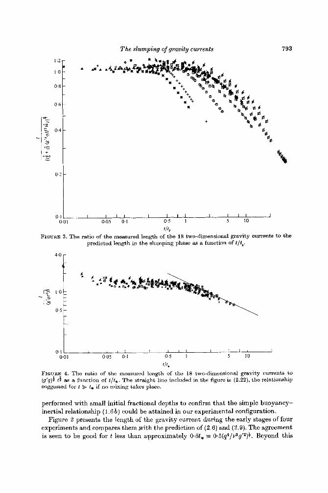
tlt, FIGURE 7. The ratio of the measured length of the nine axisymmetric gravity currents

to the predicted length in the slumping phase as a function of t/t,.

1 I 1 I I I 1 I I I I J

0.05 0.1 0.5 1 5 10

tlt. FIQURE 8. The ratio of the measured length of the nine axisymmetric gravity currents

to ( g ' ~ ) t t4 as a function of t/t,.

(b ) Axis ymmetric

Our experiments were conducted in a sector of 12" with a length of 3.5 m and a height of 18 cm. The procedure was as outlined above for the two-dimensional experiments. Because the influence of varying the initial fractional depth had already been fully investigated in the two-dimensional channel, we carried out all the axisymmetric experiments with an initial fractional depth of 1.0 (h,, = H ) . Table 2 lists the parameters of all the experiments.

We plot the results of four typical experiments in figure 6 and compare these with (2.12) and (2.14). The agreement is seen to be good. In figure 7 we plot the measured values of R/[Rt +@r-*(gt3&H2)*t]f as a function of t/ts. The vadues are seen to cluster


around 1.0 for t / t s < 1, although not as closely as for the two-dimensional results in figure 3.

In figure 8 we present the measured values of rl(g'Qt2)' as a function of t / t , . The relatively constant value for t between approximately 0.5t, and t , is evident, in agreement with (2 .15) . The length of the sector in which we conducted our experiment was, unfortunately, not sufficient for viscous effects to become appreciable. Thus no comparison with (2 .23) is possible.

4. Discussion The analysis we have presented rests on two simple ideas: that a gravity current

slumps through a series of two-dimensional rectangles or axisymmetric disks of equal volume and that the collapse is controlled a t the head and can be described by a steady-state Froude number relationship which is a function of the fractional depth. Using these ideas, we are able to predict the position of the front of the current as a function of time, which agrees well with our experiments and those of Keulegan (1957).

The appropriateness of the first assumption, that the depth of the current does not vary along its length, can be judged from figures 9 and 10. Figure 9 (plate l), presents four shadowgraph views of a two-dimensional slumping current. In the first view, the lighter (undyed) fluid has not yet reached the back wall and there is a clear variation in depth of the intruding gravity current. The depth of the current is tending towards uniformity in the second view and is satisfyingly uniform in the third view. In the fourth view, the head of the current is beyond the picture but, except for a depression near the end wall, the current is of fairly constant depth.

Similar remarks can be made about the three views of the axisymmetric slumping current in figure 10 (plate 2 ) . The depression near the apex is possibly larger than in the two-dimensional case, but its effect will be less because of the geometric predomi- nance of large radius.

A set of two-dimensional experiments, similar to those discussed in 5 3 (a), has been performed for a gravity current flowing out along a free surface. The results are somewhat unsatisfactory, and this is why they will not be discussed a t length here, because of the effect of the different surface tension of the two fluids. While the fractional difference is only a few per cent, it appeared on the scale of our experiments to have a considerable influence on the propagation speed of the current. We ascertained this by carrying out a series of experiments with fluids containing different solutes, and hence different surface tensions, keeping all other parameters constant. However, guided by the experimental results for gravity current heads under a free surface contained in Britter & Simpson (1978) , we anticipate that multiplying the right-hand side of (2.1) by 1.3 will lead, using the approach of 5 2, to satisfactory predictions. We hope to take up this matter and that of the influence of surface tension in a subsequent paper.

As mentioned previously, mixing between the two fluids has not been considered. The slumping phase occurs over a sufficiently short time scale that the effects of mixing are likely to be of secondary importance. During the subsequent inertial phase, if this occurs, the effects of mixing can increase, though its influence on the length of the gravity current is kept small because the density, as expressed in g', appears in the


combination g‘Q or g’q which remains constant. The effects of mixing during the viscous-buoyancy phase await investigation.

We wish to thank Professor M. S. Longuet-Higgins for allowing us to use his Plexiglas channel, Dr Joyce Wheeler for carrying out most of the data reduction associated with this work and preparing the figures and R. E. Britter, P. F. Linden and J. S. Turner for critical comments on a first draft of this paper. The research has been supported by grants from the Ministry of Defence, Procurement Executive (to HEH) and from the Science Research Council and the Central Electricity Generating Board (to JES).

REFERENCES

BENJAMIN, T. B. 1968 Gravity currents and related phenomena. J . Fluid Mech. 31, 209-248. BRITTER, R. E. & SIMPSON, J. E. 1978 Experiments on the dynamics of a gravity current head.

J . Fluid Mech. 88, 223-240. FANNELOP, T. K. & WALDMAN, G. D. 1971 The dynamics of oil slicks - or ‘creeping crude’.

FAY, J. A. 1969 The spread of oil slicks on a calm sea. In Oil on the Sea (ed. D . P. Hoult),

HOULT, D. P. 1972 Oil spreading on the sea. Ann. Rev. Fluid Mech. 4, 341-368. KARMAN, T. VON 1940 The engineer grapples with nonlinear problems. Bull. Am. Math. SOC.

KEULEQAN, G . H. 1957 An experimental study of the motion of saline water from locks into

SIMPSON, J. E. & BRITTER, R. E. 1979 The dynamics of the head of a gravity current advancing

SIMPSON, J. E., MILFORD, D. A. & MANSFIELD, J. R. 1977 Inland penetration of sea-breeze

A.I.A.A. J . 41, 1-10.

pp. 53-63. Plenum.

46, 615-683 (see also Collected Works, vol. IV, pp. 34-93).

fresh water channels. Nut. Bur. Stand. Rep. 5168.

over a horizontal surface. J. Fluid Mech. 94, 477-495.

fronts. Quart. J . Roy. Met. Soc. 103, 47-76.

Journal ofPluid Mechanics, Vol. 99, part 4 Plate 1

FIGURE 9. A two-dimensional gravity current with h, = H = 10 cin, I, = 30 cm, gf = 11.3cm s - ~ at approximately 4.4, 6.8, 9.7 and 17.5 s after release. The thin vertical lines are at 10 cm intervals and the end wall can just be seen on the far left. The gravity current is in the slumping phase in each view.

HUPYERT AND SIMPSON (Facing p . 800)

Plate 2

FIGXJRZ 10. An axispimetric gravity current with h0 = H = 17 ern, R, = 25 cm, 9' = 3 2 . 3 ~ r n s - ~ a t approximately 2 . 8 , 5.3 and 7.7 s after release. The apex of tlic sector can just be seen to the far left. The gravity current is in the slumping phase in tlia first two views arid in the inert,ia- buoyarxy phase in the third.

the slumping of gravity currents

Documents