Unclassified ECO/WKP(2000)3

Organisation de Coopération et de Développement Economiques OLIS : 19-Jan-2000Organisation for Economic Co-operation and Development Dist. : 27-Jan-2000__________________________________________________________________________________________

English text onlyECONOMICS DEPARTMENT

THE SIZE AND ROLE OF AUTOMATIC FISCAL STABILIZERS IN THE 1990sAND BEYOND

ECONOMICS DEPARTMENT WORKING PAPERS N0. 230

byPaul van den Noord

Unclassified

EC

O/W

KP

(2000)3E

nglish text only

Most Economics Department Working Papers beginning with No. 144 are now availablethrough OECD’s Internet Web site at http://www.oecd.org/eco/eco.

86452

Document complet disponible sur OLIS dans son format d’origine

Complete document available on OLIS in its original format

ECO/WKP(2000)3

2

ABSTRACT/RÉSUMÉ

The Size and Role of Automatic Fiscal Stabilisers in the 1990s and Beyond

This paper assesses to what extent some components of government budgets affected by themacroeconomic situation operate to smooth the business cycle in individual OECD countries. It is shownthat these automatic fiscal stabilisers have generally reduced cyclical volatility in the 1990s. However, insome countries the need to undertake fiscal consolidation in order to improve public finances has forcedgovernments to take discretionary actions that have reduced, or even offset, the effect of automatic fiscalstabilisers. This paper also shows that, by preventing sharp economic fluctuations, fiscal stabilisers mayraise long-term economic performance and avoid frequent changes in spending or tax rates. However, theyshould be employed symmetrically over the cycle in order to avoid costly debt accumulation.

JEL classification: E62, H30, H60Keywords: fiscal policy, automatic stabilisers, business cycle, public finances

*****

Ce papier évalue dans quelle mesure certaines composantes des budgets publics affectées par lasituation macroéconomique contribuent à lisser les cycles économiques dans chaque pays de l’OCDE.L’analyse montre qu’au cours de la dernière décennie ces stabilisateurs automatiques ont généralement eutendance à réduire la variabilité conjoncturelle. Cependant, dans certains pays, la nécessité d’assainir lesfinances publiques a conduit les gouvernements à prendre des mesures discrétionnaires qui ont réduit, voireannulé, les effets des stabilisateurs automatiques. Ce papier montre aussi qu’en empêchant de trop fortesfluctuations économiques, les stabilisateurs automatiques peuvent accroître la performance économique àlong terme et éviter des variations des dépenses ou des taux d’imposition trop fréquents. Ils doiventtoutefois être utilisés de manière symétrique au cours du cycle pour éviter un accroissement coûteux duniveau d’endettement.

Classification JEL: E62, H30, H60Mots-clés: politique budgétaire, stabilisateurs automatiques, cycle économique, finances publiques

Copyright OECD, 2000

Applications for permissions to reproduce or translate all, or part of, this material should be madeto: Head of Publications Service, OECD, 2 rue André Pascal, 75775 Parix Cedex 16, France.

ECO/WKP(2000)3

3

Table of Contents

Page

I. Introduction .................................................................................................................................4

II. How large are automatic fiscal stabilisers? .................................................................................5

III. What impact do automatic fiscal stabilisers have on the economy? ...........................................8

IV. Do automatic fiscal stabilisers have an impact on longer-term performance?..........................12

Appendix ..................................................................................................................................................17

References ................................................................................................................................................29

ECO/WKP(2000)3

4

THE SIZE AND ROLE OF AUTOMATIC FISCAL STABILISERS IN THE 1990S AND BEYONDPaul van den Noord1

I. Introduction

1. Many components of government budgets are affected by the macroeconomic situation in waysthat operate to smooth the business cycle, i.e. they act as “automatic stabilisers”. For example, in arecession fewer taxes are collected, which operates to support private incomes and damps the adversemovements in aggregate demand. Conversely, during a boom more taxes are collected, counteracting theexpansion in aggregate demand. This stabilising property is evidently stronger if the tax system is moreprogressive. Another automatic fiscal stabiliser is the unemployment insurance system: in a downswing thegrowing payment of unemployment benefits supports demand and vice versa in an upswing.

2. The impact of automatic fiscal stabilisers may, at varying degrees, be reinforced by othermechanisms that operate to smooth the business cycle. For example, the behaviour of imports is sensitiveto short-term fluctuations in aggregate demand and therefore help to stabilise variations in economicactivity. Similarly, “permanent income” theories of consumption behaviour suggest that consumerspending responds only slowly to income fluctuations, which would tend to make private saving behaviourstabilising. On the other hand, saving behaviour can be destabilising, when a slowing economy leads tohigher saving to build up reserves as a precaution against weaker earnings prospects and job security.Capital gains and losses on real and financial assets may also lead to destabilising movements in privatesaving. Reactions in financial markets and of monetary conditions to cyclical developments should alsoreinforce the fiscal stabilisation mechanisms. Indeed, estimates for the United States suggest thatstabilisation through financial markets’ reactions offset as much as 60 per cent of the cyclical variations inoutput, see Asdrubali et al. (1996). The role of monetary policy is central in this regard, although thisdepends crucially on the exchange rate regime in place. Where exchange rate arrangements permit,monetary policy adjustments designed to ensure price stability should operate to stabilise activity bygenerating pro-cyclical interest rate developments and at least working to encourage pro-cyclical exchangerate behaviour in a way that provides incentives for further adjustment in international trade flows. Under afixed exchange rate regime, on the other hand, monetary policy is not available to play such a role and, insome circumstances (e.g. several countries participating in or shadowing the ERM in the early 1990s), mayeven be destabilising. Finally, cyclical variations in labour productivity prevent sharp swings in thedemand for labour and thus help to stabilise unemployment.

3. Although by damping the business cycle automatic fiscal stabilisers may help to reduce the long-lasting economic damage associated with large under-utilised resources, they also entail risks for theeconomy. One relates to the importance of allowing stabilisers to operate symmetrically over the businesscycle. If governments allow automatic fiscal stabilisers to work fully in a downswing but fail to resist thetemptation to spend cyclical revenue increases during an upswing, the stabilisers may lead to a bias toward 1 . The author is indebted to Paul Atkinson, Jørgen Elmeskov, Mike Feiner and Ignazio Visco and several

other colleagues in the Economics Department for comments and drafting suggestions, to Dave Rae forrunning simulations with the INTERLINK model and Anne Eggimann, Isabelle Duong, Nanette Mellageand Chantal Nicq for technical assistance. Special thanks are due to Marco Buti and several nationaldelegates for stimulating discussions. Of course all errors and omissions are the author’s.

ECO/WKP(2000)3

5

weak underlying (or “structural”) budget positions. The result may be rises in public indebtedness duringperiods of cyclical weakness that are not subsequently reversed when activity recovers. This, in turn, couldlead to higher interest rates as well as requiring higher taxes (or spending reductions) to finance debtservicing. Unstable “debt dynamics” working to increase debt-GDP ratios over time, due to real interestrates that exceed economic growth rates, may aggravate this problem. A second risk arises from the factthat automatic fiscal stabilisers respond to structural changes in the economic situation as well as tocyclical developments. Consequently, if the economy’s growth potential declines, and this is notappreciated by the government in a timely fashion, the operation of automatic fiscal stabilisers is likely toundermine public finance positions that might otherwise have been sound. Finally, automatic fiscalstabilisation results from the operation of tax and benefit systems that primarily serve other objectives suchas income security and redistribution. These systems may delay necessary adjustment in the wake of arecession, thus contributing to poor economic performance.

4. Against this backdrop this paper assesses the size and role of automatic fiscal stabilisers in the1990s and beyond. The next section below provides estimates of the size of automatic fiscal stabilisation asmeasured by the cyclical component of the budget balance over the past decade. The following sectionsfocus on the impact of automatic fiscal stabilisers on the business cycle and on longer-run economicperformance. The appendix describes the analytical framework that has been developed to measure thesensitivity of government net lending to cyclical variations in GDP, as well as the key parameters andestimates of this sensitivity for most OECD countries.

II. How large are automatic fiscal stabilisers?

5. The counter-cyclical demand impulse stemming from automatic fiscal stabilisers depends on thesensitivity of government net lending, as a share of GDP, to cyclical variations in output, and the size ofthose variations. Measurement is largely an unsettled issue. Widely different methods are being employedboth by national governments and various international institutions (see Box 1). Each method has specificstrengths and weaknesses, but whatever method is employed, the user needs to be aware of a problem of“simultaneity”: the business cycle changes the fiscal position which, in turn, affects economic activity. TheOECD Secretariat’s approach involves three main steps:

(i) Elasticities of various forms of taxation and expenditure with respect to output arecalculated to estimate the sensitivity of these items to the cycle. These have been updatedfor the purpose of this paper (see the appendix). On the revenue side, all tax receipts areadjusted for the cycle, with taxes being grouped into four types (indirect, business, socialsecurity and personal income tax). On the expenditure side, estimates of the automaticstabilisers are limited to the impact of the cycle on benefits paid to the unemployed(including “active labour market measures”), although debt-interest payments are alsosensitive to some extent. The new elasticities are reported in Table A.1 of the annex.

(ii) Potential output is estimated on the basis of country-specific production functions thathave been estimated for a sample period covering the past three decades. This work waspreviously reported in Giorno et al. (1995), and has been updated since.

(iii) The output gap and the elasticities are used to derive the impact on tax and expenditurearising from the economy’s operation above or below potential. This is taken to measurethe cyclical component of each item. Combining these estimates gives the full cyclicalcomponent of the budget balance and allows the simultaneous calculation of thecyclically-adjusted budget balance, i.e. the general government net borrowing or lendingthat would take place if the economy were operating at potential.

ECO/WKP(2000)3

6

Box 1. Gauging fiscal automatic stabilisers -- different approaches

Different approaches have been developed over time to disentangle cyclical and structural components of governmentexpenditure, (tax) revenues and balances. Most approaches start off from the observation that economic activity influences taxbases (wage bill, profits, consumption, etc.) and unemployment, which, in turn determine tax proceeds and public expenditure. Theapproaches differ with respect to the method employed to identify the cycle in economic activity and the way to determine thesensitivity of budget items to the cycle. The official methods also differ from one country to another.

Generally speaking, two ways to identify the cycle in economic activity co-exist. A mechanical approach usessmoothing devices (such as Hodrick-Prescott filters) to establish a trend level of output; the cyclical component (output gap) is thedifference between actual and trend output. In some cases the de-trending of output series is dropped altogether, with thesmoothing device applied directly to the tax base and unemployment series. The mechanical approach is relatively simple,transparent and requires little judgmental intervention. A major drawback is the “end point bias”: the difference between actual andtrend series tends to become small for recent observations, meaning that economic slack or overheating may escape the observer.This drawback has motivated the development of an alternative approach measuring potential rather than trend output, based on aproduction function. This method, which has been adopted by the OECD Secretariat, is somewhat more complex since it requiresjudgements on the rate of technological change, its bias (labour or capital augmenting) and, importantly, the rate of structuralunemployment. However, it is less susceptible to the end-point problem for recent observations.

Methods to determine the sensitivity of budget items to the cycle can be grouped into three categories:

- A first approach is to run regressions on the observed tax proceeds and public expenditure, with as explanatoryvariables, discretionary changes in tax or benefit parameters, a trend and a cyclical term (the latter two may bebased on trend or potential output measures). From these equations elasticities are derived that measure the impactof a (cyclical) change in output on tax revenues or expenditure (see for an example, Bismut 1995). The accuracyof this approach strongly depends on the reliability of the policy variables that are included in the regressions. Ifthese fail to cover the whole ground of relevant policy measures, some of the policy-induced effects on the budgetmay end up in the estimated elasticities, which could therefore be misleading. This approach will only be fruitfulif detailed information on relevant policy changes is available for a long range of years and kept up to date. Thecollection of such information is time consuming and this approach is therefore less suited for users that need tocover a large number of countries.

- A second group of methods derive tax and expenditure elasticities from a macro-econometric model, withstandard-shock simulations calibrated to show the impact of a 1 per cent (cyclical) increase in output on budgetvariables. This approach has the advantage that it allows differentiating between various kind of demand shocks(consumption, exports, etc.). On the other hand, it does not resolve the data collection problem alluded to above,because, in order to give accurate results for this purpose, the tax and expenditure equations in the model need tobe estimated according to the above procedure.

- A third approach, which has been adopted by the OECD Secretariat (see the appendix), proceeds in three steps.First, the elasticities of the relevant tax bases and unemployment with respect to (cyclical) economic activity,i.e. the output gap, are estimated through regression analysis. Next, the elasticities of tax proceeds or expenditurewith respect to the relevant bases are extracted from the tax code or simply set to unity in cases whereproportionality may be assumed. These two sets of elasticities are subsequently combined into reduced-formelasticities that link the cyclical components of taxes and expenditure to the output gap. While this method aims tostrike a balance between accuracy and resource cost, it does not allow a further breakdown of the structural fiscalbalance into discretionary and induced components.

In addition the OECD Secretariat has experimented with a complementary approach, using a structural VAR model tocapture the effects on fiscal balances of specific economic shocks in the past in EU countries (Dalsgaard and De Serres, 1999). Amain advantage relative to the above approaches is that estimates of output gaps are not required, but the results with this modelare not directly comparable to those derived from other approaches. This is the case because the elasticities that are derived fromthe VAR model include not only the impact of automatic stabilisers, but also that of discretionary fiscal policy to the extent that itreacts in a systematic fashion to economic disturbances.

ECO/WKP(2000)3

7

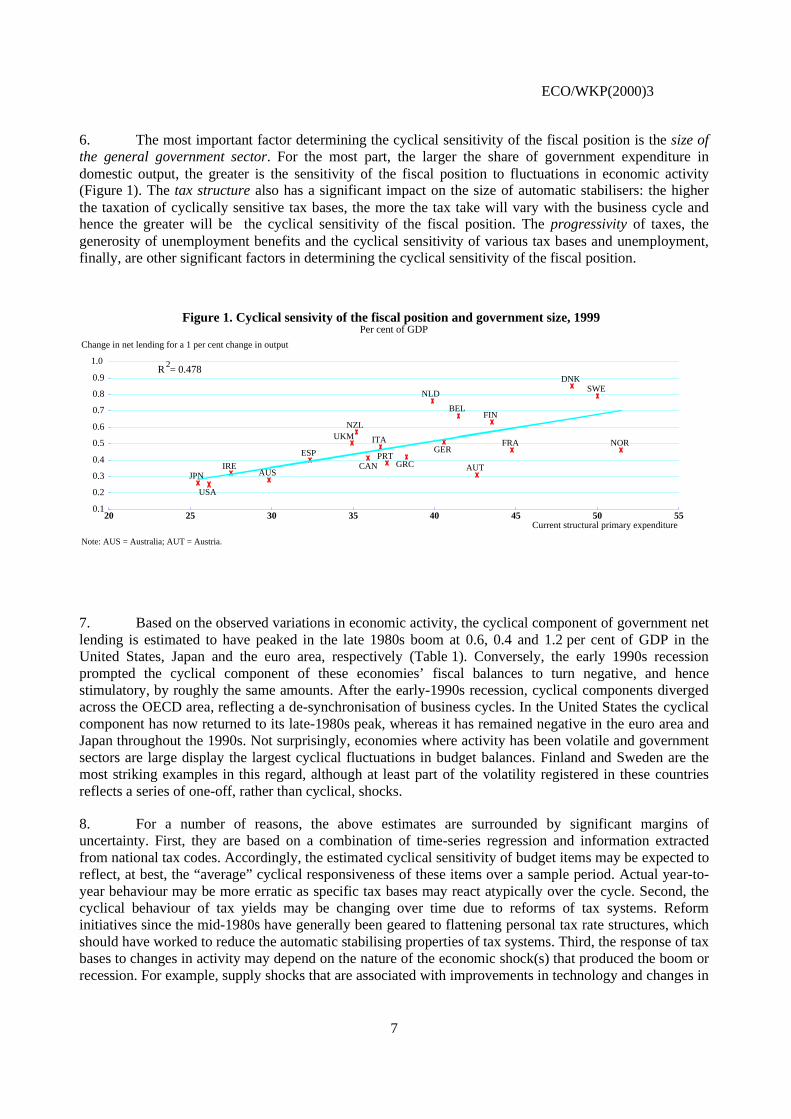
6. The most important factor determining the cyclical sensitivity of the fiscal position is the size ofthe general government sector. For the most part, the larger the share of government expenditure indomestic output, the greater is the sensitivity of the fiscal position to fluctuations in economic activity(Figure 1). The tax structure also has a significant impact on the size of automatic stabilisers: the higherthe taxation of cyclically sensitive tax bases, the more the tax take will vary with the business cycle andhence the greater will be the cyclical sensitivity of the fiscal position. The progressivity of taxes, thegenerosity of unemployment benefits and the cyclical sensitivity of various tax bases and unemployment,finally, are other significant factors in determining the cyclical sensitivity of the fiscal position.

Figure 1. Cyclical sensivity of the fiscal position and government size, 1999Per cent of GDP

20 25 30 35 40 45 50 550.1

0.2

0.3

0.4

0.5

0.6

0.7

0.8

0.9

USA

JPN

GERFRAITAUKM

CANAUS

AUT

BEL

DNK

FIN

GRCIRE

NLD

NZL

NOR

PRTESP

SWE

Change in net lending for a 1 per cent change in output

Current structural primary expenditure

1.0R = 0.4782

Note: AUS = Australia; AUT = Austria.

7. Based on the observed variations in economic activity, the cyclical component of government netlending is estimated to have peaked in the late 1980s boom at 0.6, 0.4 and 1.2 per cent of GDP in theUnited States, Japan and the euro area, respectively (Table 1). Conversely, the early 1990s recessionprompted the cyclical component of these economies’ fiscal balances to turn negative, and hencestimulatory, by roughly the same amounts. After the early-1990s recession, cyclical components divergedacross the OECD area, reflecting a de-synchronisation of business cycles. In the United States the cyclicalcomponent has now returned to its late-1980s peak, whereas it has remained negative in the euro area andJapan throughout the 1990s. Not surprisingly, economies where activity has been volatile and governmentsectors are large display the largest cyclical fluctuations in budget balances. Finland and Sweden are themost striking examples in this regard, although at least part of the volatility registered in these countriesreflects a series of one-off, rather than cyclical, shocks.

8. For a number of reasons, the above estimates are surrounded by significant margins ofuncertainty. First, they are based on a combination of time-series regression and information extractedfrom national tax codes. Accordingly, the estimated cyclical sensitivity of budget items may be expected toreflect, at best, the “average” cyclical responsiveness of these items over a sample period. Actual year-to-year behaviour may be more erratic as specific tax bases may react atypically over the cycle. Second, thecyclical behaviour of tax yields may be changing over time due to reforms of tax systems. Reforminitiatives since the mid-1980s have generally been geared to flattening personal tax rate structures, whichshould have worked to reduce the automatic stabilising properties of tax systems. Third, the response of taxbases to changes in activity may depend on the nature of the economic shock(s) that produced the boom orrecession. For example, supply shocks that are associated with improvements in technology and changes in

ECO/WKP(2000)3

8

labour supply may coincide with demand shocks that stem from the international trade cycle or movementsin household sentiment. In theory, the change in the fiscal position that results from a supply shock isrecorded as structural rather than cyclical. In practice, however, it is not allways easy to disentanglestructural and cyclical influences on the budgets.

Cyclical peak Subsequent trough Current situation

YearOutput

gapCyclical

component YearOutput

gapCyclical

component YearOutput

gapCyclical

componentUnited States 1989 2.0 0.6 1991 -1.8 -0.6 1999 2.5 0.6 Japan 1991 3.1 0.4 1995 -2.3 -0.5 1999 -3.5 -0.9 Germany 1990 2.8 1.3 1993 -1.0 -0.5 1999 -1.7 -0.9 France 1990 1.2 0.5 1993 -2.3 -1.1 1999 -0.7 -0.3 Italy 1989 1.9 0.9 1993 -3.2 -1.7 1999 -3.2 -1.5 United Kingdom 1988 5.6 2.8 1992 -2.8 -1.6 1999 0.7 0.4 Canada 1988 4.0 1.7 1992 -4.6 -2.3 1999 0.1 0.0

Australia 1989 2.1 0.6 1992 -2.8 -0.9 1999 1.2 0.3 Austria 1990 2.7 0.8 1993 -1.5 -0.5 1999 0.3 0.1 Belgium 1990 2.0 1.3 1993 -2.9 -2.1 1999 -1.2 -0.8 Denmark 1986 3.0 2.6 1993 -4.7 -4.1 1999 0.1 0.1 Finland 1989 5.9 3.4 1993 -9.2 -7.2 1999 0.4 0.3 Greece 1989 2.9 1.3 1994 -2.7 -1.2 1999 -0.6 -0.2

Ireland 1990 4.6 1.8 1994 -4.0 -1.6 1999 5.0 1.6 Netherlands 1990 1.7 1.5 1993 -1.1 -1.0 1999 1.4 1.1 New Zealand 1986 1.9 1.3 1992 -5.2 -3.2 1999 -1.6 -0.9 Norway (mainland) 1986 2.7 1.6 1990 -4.6 -3.1 1999 1.4 0.6 Portugal 1990 3.4 1.2 1994 -1.8 -0.7 1999 -0.1 0.0 Spain 1990 4.7 1.9 1996 -2.0 -0.8 1999 0.2 0.1 Sweden 1989 4.4 3.4 1993 -5.9 -5.4 1999 -0.2 -0.1

Euro area average 1990 2.4 1.2 1993 -1.9 -1.0 1999 -1.1 -0.5

OECD average2 1989 1.8 0.9 1993 -1.8 -0.5 1999 0.1 0.0

1. The cyclical component is calculated by subtracting the structural component, as a per cent of potential GDP, from the actual balance, as a per cent of GDP. The structural component in turn is calculated from the cyclically-adjusted tax revenues and government expenditures, based on the ratio of potential output to actual output and assumed built-in elasticities (see Appendix).2. Excluding Czech Republic, Hungary, Iceland, Korea, Mexico, Poland, Switzerland and Turkey.

Source : OECD.

Table 1. Cyclical component of general government financial balances1

Surplus (+) or deficit (-) as a per cent of GDP

III. What impact do automatic fiscal stabilisers have on the economy?

9. A change in cyclically sensitive government spending (mainly unemployment benefits) or taxesaffects spending in the economy mainly through its impact on disposable income, and hence householdconsumption. The Secretariat’s INTERLINK model captures the basic macroeconomic relationships thatoperate, and simulations have been carried out with this model to assess the degree to which automaticfiscal stabilisers have damped cyclical fluctuations over the 1990s. Fiscal stabilisers have been “switchedoff” in the simulations by setting tax and spending flows to their structural levels. Monetary policy isassumed to have responded to economic developments in much the same way as it has usually behavedhistorically, i.e. leaning against the business cycle to some extent. In practical terms this has been

ECO/WKP(2000)3

9

approximated by a “Taylor rule”, which implies that interest rates are raised if either inflation or the outputgap rise above their baseline levels, in all countries except for those (other than Germany) that participatedin the ERM throughout the 1990s until the start of monetary union and were least affected by theturbulence of the early and mid-1990s (i.e. France, Austria, Belgium, Denmark, the Netherlands andSpain). For the latter group of countries, nominal interest rates were kept constant. Nominal exchange rateswere held fixed and the simulations run on a country-by-country basis, which means that internationallinkages were switched off.

10. The simulations suggest that over the 1990s the automatic fiscal stabilisers have worked to dampthe cyclical fluctuations in economic activity by roughly a quarter on average (Figure 2). However, there isconsiderable cross-country variation, in part reflecting the relative openness of economies and differencesin monetary policy responsiveness. In particular, Finland and Denmark provide clear examples whereautomatic fiscal stabilisers are essential: without them, output volatility in the 1990s would have beentwice as high. The ranking of countries with regard to the stabilising impact of automatic fiscal stabilisersreported in Figure 2 is broadly in line with other studies, but some studies report somewhat higher levels ofstabilisation for the European countries; see for example Buti and Sapir (1998).

Figure 2. Impact of automatic fiscal stabilisers

0.0

0.5

1.0

1.5

2.0

2.5

0

2

4

6

8

10

12

14

FIN DNK GER UKM NLD SWE NZL ITA BEL CAN NOR ESP USA AUS FRA GRC JPN IRE AUT

1

Root mean square of the output gap with automatic fiscal stabilisers (A) (right scale)Root mean square of the output gap without automatic fiscal stabilisers (B) (right scale)Ratio between (B) and (A) (left scale)

22

1. Unchanged nominal exchange rates for all countries and a Taylor rule for interest rates for all countries except France, Austria,Belgium Denmark, the Netherlands and Spain, where interest rates were kept unchanged.

2. Defined as 2

2000

19919

1t

t

gap∑=

where gapt = (y - y*)/y*; y = GDP and y* = potential GDP.

ECO/WKP(2000)3

10

11. There are important qualifications to these results. First, where fiscal positions threatened tobecome unsustainable, even if this was due to cyclical weakness, business and financial market confidencedeteriorated in a number of countries. Therefore risk premia in real long-term interest rates rose (Orr et al.,1995), which had a negative influence on economic activity. When this occurs, the negative effect onprivate spending operates to diminish or even to reverse the supportive effects of automatic fiscalstabilisers. Such confidence effects are not incorporated in INTERLINK and, therefore, not reflected in theresults reported in Figure 2. When financial markets respond to rising budget deficits this way, there islittle alternative to correcting the fiscal position even if this means overriding the automatic stabilisers.Several cases have been reported where such policy responses helped to reverse increases in long-terminterest rates and contributed to a brisk recovery, notably in Finland, Denmark, Ireland and Sweden (seeGiavazzi and Pagano, 1990 and 1995).

12. Second, the model simulations may also understate the extent of “non-Keynesian” responses tofiscal automatic stimulus, by which is meant an increase in household saving rates in reaction todeteriorating fiscal balances. If this occurs, the demand impetus stemming from the fiscal automaticstabilisers may be smaller than expected or even negative. Such “perverse” savings reactions are all themore likely if public debt is already high, since the private sector may fear tax increases further down theroad to offset a debt explosion (Sutherland, 1997). In Europe, for instance, the intense public debates priorto the ratification of the Maastricht Treaty have made the public well aware of fiscal issues, and may thushave prompted such forward-looking saving behaviour (Martinot, 1999). This could happen again if, forexample, the public deficit approaches the 3 per cent of GDP benchmark in a future recession.Unfortunately, while forward-looking saving behaviour invalidates the impact of fiscal automaticstabilisers on economic activity, the adverse impact on government borrowing remains.

13. The simulations described above treat discretionary fiscal policy adjustments as if they were notinfluenced either by the operation of automatic stabilisers or by the situation in the economy. However, theoverall degree of fiscal stabilisation reflects both the operation of the stabilisers themselves and theirinfluence on, and interaction with, discretionary policies. Thus, if automatic stabilisers are overridden bydiscretionary adjustments, their impact will be neutralised. On the other hand, if they are reinforced bydiscretionary adjustments, the overall fiscal impulse will be stronger. Table 2 reports both the behaviour offiscal policy and the impact of automatic stabilisers on budget balances over the past decade. It suggeststhat in the early-1990s recession twelve countries reinforced the automatic fiscal stabilisers through aneasy stance of fiscal policy (United States, Japan, France, United Kingdom, Canada, Australia, Austria,Denmark, Finland, Norway, Portugal and Sweden) while other countries offset the working of automaticfiscal stabilisers by adopting a tight fiscal stance. As a result, on average the fiscal stance in the OECDarea, as measured by the change in the structural primary balance, was neutral in the recession. With theexceptions of Japan and Norway, all countries reverted to or maintained a tight fiscal stance during theremainder of the decade.

14. A scenario simulated with INTERLINK in which a neutral fiscal stance is assumed for the 1990ssuggests that the use of discretionary fiscal policy on average slashed the fluctuations in economic activityduring the decade by half (Table 3). Interestingly, the United States obtained this result while achieving abetter fiscal position than it otherwise would have realised. Discretionary fiscal policy thus acted as apowerful complement to automatic fiscal stabilisation; it contributed to both a virtuous circle of sustainableeconomic growth and steadily improving public finances. In Japan the variability of economic activity hasalso been significantly limited as a result of discretionary fiscal policy. However, since both automatic anddiscretionary fiscal policy have been mostly stimulatory over the decade they caused a dramaticdeterioration of the fiscal position and the public debt-to-GDP ratio.

ECO/WKP(2000)3

11

Overall balance Cyclical component Structural primary balance

Late-1980s peak to early-1990s trough

Early-1990s trough to 1999

Late-1980s peak to early-1990s trough

Early-1990s trough to 1999

Late-1980s peak to early-1990s trough

Early-1990s trough to 1999

United States -1.8 7.3 -1.1 1.2 -1.1 4.6 Japan -6.5 -4.0 -0.9 -0.4 -5.5 -2.9 Germany -1.2 1.6 -1.8 -0.4 1.1 2.5 France -4.4 3.8 -1.6 0.8 -2.2 3.1 Italy 0.4 7.1 -2.6 0.2 5.8 2.4 United Kingdom -7.1 7.2 -4.4 2.0 -3.6 6.1 Canada -4.9 9.6 -4.0 2.4 -0.5 7.2

Australia -5.9 6.7 -1.5 1.3 -1.8 4.5 Austria -1.7 2.0 -1.3 0.6 -0.1 1.4 Belgium -1.8 6.2 -3.4 1.3 1.4 2.2 Denmark -6.2 5.8 -6.7 4.2 -1.4 0.3 Finland -13.2 10.2 -10.5 7.4 -1.7 4.5 Greece 4.4 8.5 -2.5 1.0 12.8 2.5

Ireland 0.8 5.4 -3.4 3.3 2.2 -0.3 Netherlands 2.1 3.0 -2.5 2.1 4.8 0.5 New Zealand 3.3 3.2 -4.4 2.2 5.9 -1.9 Norway (mainland) -6.2 2.4 -4.7 3.7 -3.0 0.9 Portugal -0.9 4.2 -1.9 0.6 -3.1 0.7 Spain -0.9 3.6 -2.8 0.9 3.5 1.5 Sweden -17.0 14.1 -8.8 5.3 -7.8 10.9

Euro area average -1.4 3.9 -2.2 0.5 1.4 2.7

OECD average2 -3.0 3.6 -1.4 0.5 0.0 1.4

1. The cyclical component and the structural primary balance do not add up to the overall balance, the net interest payments being the residual.2. Excluding Czech Republic, Hungary, Iceland, Korea, Mexico, Poland, Switzerland and Turkey.

Source : OECD.

Table 2. Automatic fiscal stabilisers and the fiscal stancePercentage of (potential) GDP

Change in1

15. The simulations suggest that in the European Union the tight stance of discretionary fiscal policycontributed to the sluggishness of the recovery from the 1993 recession. However, there was no otheroption in many EU countries given the poor state of public finances at the time of the Maastricht Treatyand beyond. Had fiscal automatic stabilisers been allowed to work without any discretionary adjustmentsin the euro area, the simulations suggest that 1999 budget deficits would on average be six times as high astheir current levels. This would undoubtedly have boosted long-term interest rates, perhaps significantly,and would have extended the episode of exchange rate turbulence that marked the early and mid-1990s.Obviously this would have made the establishment of monetary union extremely difficult. Interestingly,several European countries that eased fiscal policy during the recession and tightened later (France, theUnited Kingdom and Sweden) had some success in terms of stabilising the economy, but at the cost offiscal positions that were still weaker in 1999 and substantially higher debt ratios.

ECO/WKP(2000)3

12

Table 3. Volatility of economic activity and public finances with and without discretionary fiscal policy 1

Root mean square of output gap

Net lending, per cent of GDP

Gross debt, per cent of GDP

1991-1999 1999 1999Fiscal stance in the

early-1990s

downturn2 Actual

Neutral discretionary fiscal policy Actual

Neutral discretionary fiscal policy Actual

Neutral discretionary fiscal policy

United States easy 1.4 3.8 1.0 -5.0 62.4 76.2 Japan3 easy 2.3 4.6 -6.0 16.3 97.3 22.9 Germany tight 1.3 1.6 -1.6 -6.5 62.6 72.7 France easy 1.8 1.7 -2.2 -0.6 65.2 48.9 Italy tight 2.1 0.4 -2.3 -28.0 119.7 187.5 United Kingdom easy 1.5 1.9 0.7 1.6 54.0 31.5 Canada easy 2.7 1.9 1.6 -37.8 86.9 192.7

Australia easy 1.7 3.4 0.6 6.2 30.3 0.0 Austria easy 1.8 3.2 -2.1 -6.8 63.3 80.4 Belgium tight 1.8 1.1 -1.0 -4.5 114.1 124.5 Finland easy 5.7 8.6 -3.0 2.7 43.6 26.2 Greece tight 1.8 4.4 -1.6 -13.4 108.8 152.0

Ireland tight 3.1 3.8 3.4 0.5 43.9 53.2 Netherlands tight 1.0 2.5 -0.6 -6.5 62.9 86.2 New Zealand tight 2.8 3.2 0.0 0.6 ** **Spain tight 1.9 3.0 -1.4 -7.9 70.3 86.6 Sweden easy 2.9 4.0 2.3 2.5 68.3 42.2

Euro area average4 tight 1.4 0.6 -1.6 -9.6 74.8 95.3

OECD average5 neutral 0.8 1.6 -1.0 -3.5 72.7 73.6

1. Neutral discretionary fiscal policy means holding structural tax and primary spending at their 1990 levels (as a proportion of potential GDP). The monetary policy assumption is an unchanged nominal exchange rate for all countries, and a Taylor rule for interest rates for all countries except France, Austria, Belgium, the Netherlands and Spain (their nominal interest rates were kept unchanged). For technical reasons, results for Denmark, Norway and Portugal are not available.2. Based on the change in the structural primary balance as a percent of potential GDP between the late-1980s cyclical peak and the early-1990s cyclical trough (an increase in the balance points to a tight fiscal stance and vice versa, see Table 2).3. Simulation ends in 1998. For technical reasons results for 1999 are not available.4. Excluding Portugal.5. Excluding Czech Republic, Denmark, Hungary, Iceland, Korea, Mexico, Norway, Poland, Portugal, Switzerland and Turkey.

Source : OECD.

IV. Do automatic fiscal stabilisers have an impact on longer-term performance?

16. There are a number of ways in which fiscal stabilisers may impinge on longer-term economicperformance. On the positive side, achievement of longer-term objectives of sustainable economic growth,full employment and price stability, requires short-run macroeconomic stabilisation policy to ensure themaintenance of an appropriate level of aggregate demand. Recurrent large under-utilisation of resourcescan have damaging longer-term effects if it leads to under-investment in, and failure to maintain, physicaland, more importantly, human capital. While periods of overheating may have some similar, offsettingeffects in a favourable direction, it is likely that sharp fluctuations around the trend on balance havenegative implications for the economy’s longer-term potential (see Box 2 for a numerical experiment toillustrate this).

ECO/WKP(2000)3

13

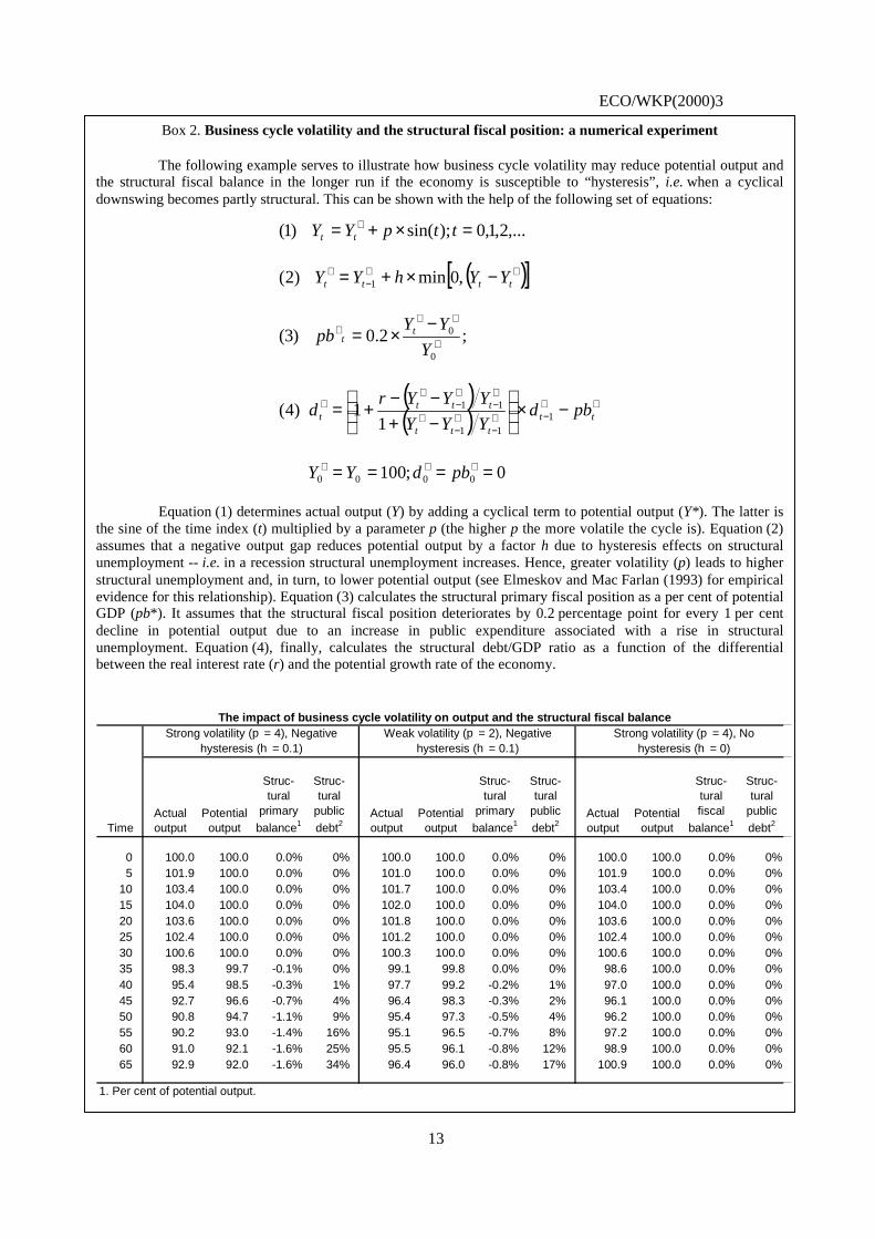
Box 2. Business cycle volatility and the structural fiscal position: a numerical experiment

The following example serves to illustrate how business cycle volatility may reduce potential output andthe structural fiscal balance in the longer run if the economy is susceptible to “hysteresis”, i.e. when a cyclicaldownswing becomes partly structural. This can be shown with the help of the following set of equations:

( )[ ]

( )( )

0;100

11)4(

;2.0)3(

,0min)2(

,...2,1,0);sin()1(

0000

111

11

0

0

1

====

−×

−+−−

+=

−×=

−×+=

=×+=

∗∗∗

∗∗−∗

−∗−

∗

∗−

∗−

∗∗

∗

∗∗∗

∗∗−

∗

∗

pbdYY

pbdYYY

YYYrd

Y

YYpb

YYhYY

ttpYY

ttttt

tttt

tt

tttt

tt

Equation (1) determines actual output (Y) by adding a cyclical term to potential output (Y*). The latter isthe sine of the time index (t) multiplied by a parameter p (the higher p the more volatile the cycle is). Equation (2)assumes that a negative output gap reduces potential output by a factor h due to hysteresis effects on structuralunemployment -- i.e. in a recession structural unemployment increases. Hence, greater volatility (p) leads to higherstructural unemployment and, in turn, to lower potential output (see Elmeskov and Mac Farlan (1993) for empiricalevidence for this relationship). Equation (3) calculates the structural primary fiscal position as a per cent of potentialGDP (pb*). It assumes that the structural fiscal position deteriorates by 0.2 percentage point for every 1 per centdecline in potential output due to an increase in public expenditure associated with a rise in structuralunemployment. Equation (4), finally, calculates the structural debt/GDP ratio as a function of the differentialbetween the real interest rate (r) and the potential growth rate of the economy.

The impact of business cycle volatility on output and the structural fiscal balanceStrong volatility (p = 4), Negative

hysteresis (h = 0.1)Weak volatility (p = 2), Negative

hysteresis (h = 0.1)Strong volatility (p = 4), No

hysteresis (h = 0)

TimeActual output

Potential output

Struc-tural

primary

balance1

Struc-tural

public

debt2Actual output

Potential output

Struc-tural

primary

balance1

Struc-tural

public

debt2Actual output

Potential output

Struc-tural fiscal

balance1

Struc-tural

public

debt2

0 100.0 100.0 0.0% 0% 100.0 100.0 0.0% 0% 100.0 100.0 0.0% 0%5 101.9 100.0 0.0% 0% 101.0 100.0 0.0% 0% 101.9 100.0 0.0% 0%

10 103.4 100.0 0.0% 0% 101.7 100.0 0.0% 0% 103.4 100.0 0.0% 0%15 104.0 100.0 0.0% 0% 102.0 100.0 0.0% 0% 104.0 100.0 0.0% 0%20 103.6 100.0 0.0% 0% 101.8 100.0 0.0% 0% 103.6 100.0 0.0% 0%25 102.4 100.0 0.0% 0% 101.2 100.0 0.0% 0% 102.4 100.0 0.0% 0%30 100.6 100.0 0.0% 0% 100.3 100.0 0.0% 0% 100.6 100.0 0.0% 0%35 98.3 99.7 -0.1% 0% 99.1 99.8 0.0% 0% 98.6 100.0 0.0% 0%40 95.4 98.5 -0.3% 1% 97.7 99.2 -0.2% 1% 97.0 100.0 0.0% 0%45 92.7 96.6 -0.7% 4% 96.4 98.3 -0.3% 2% 96.1 100.0 0.0% 0%50 90.8 94.7 -1.1% 9% 95.4 97.3 -0.5% 4% 96.2 100.0 0.0% 0%55 90.2 93.0 -1.4% 16% 95.1 96.5 -0.7% 8% 97.2 100.0 0.0% 0%60 91.0 92.1 -1.6% 25% 95.5 96.1 -0.8% 12% 98.9 100.0 0.0% 0%65 92.9 92.0 -1.6% 34% 96.4 96.0 -0.8% 17% 100.9 100.0 0.0% 0%

1. Per cent of potential output.

ECO/WKP(2000)3

14

Box 2. Business cycle volatility and the structural fiscal position: a numerical experiment (continued)

The table above shows that for p = 4 and h = 0.1 (which are arbitrarily chosen) and r = 0.02, potentialoutput will have fallen by 7 per cent by the end of the cycle and the structural balance by 1½ percentage points, whilethe potential debt/GDP ratio climbs to 34 per cent. However, if cyclical volatility is halved (p = 2), potential output,the structural balance and the structural debt ratio deteriorate by half as much.

It needs to be pointed out, however, that the experiment describes a second-best option. The first-bestoption would be to remove the sources of “hysteresis” altogether, i.e. prevent cyclical declines in output fromaffecting potential output, as is illustrated by the third simulation reported in the table.

17. Moreover, the theoretical literature strongly suggests that it is less costly to keep tax rates stableover the cycle, and hence allow automatic fiscal stabilisers to operate, than to adjust tax rates from oneyear to another. Such a policy may, in any event, prove to be ineffective if activity keeps moving asattempts are made to stabilise the fiscal position. Similar arguments will apply to adjusting spendingparameters such as unemployment benefit rates. Automatic stabilisation can also be justified on the groundthat the government faces fewer liquidity constraints and a lower risk premium than the private sector andtherefore is likely to be more efficient at consumption smoothing through cyclical downturns thanhouseholds are.

18. There is also a negative side, or at least there are risks, involved in using automatic fiscalstabilisers. First, unless care is taken to ensure that automatic stabilisers operate symmetrically over thebusiness cycle, the result may be permanently higher government indebtedness and associated servicingcost. Most importantly, this involves ensuring that the stabilisers are allowed to work in booms as well asduring slowdowns so that they do not bias structural budget positions toward deficits. However, permanenteffects can also arise for either of two further reasons: downswings and upswings can differ in terms oftheir intensity; or they can differ in terms of their duration. A second order effect can also arise as aconsequence of interest rate variations over the cycle. The risk of unsustainable debt accumulation isheightened by adverse debt dynamics that may emerge when real interest rates exceed growth rates. As aresult, debt expands at a faster rate than GDP, hence the debt-to-GDP ratio rises unless there is asufficiently large primary surplus. The long-run damage to economic growth that results from sustaininghigh public debt levels in the wake of a recession without subsequently reducing them may be substantial,because taxes, and the distortions they create, as well as real long-term interest rates would have to behigher.

19. Figure 3 decomposes the accumulation of gross public debt relative to GDP into relevantcontributing factors according to the following identity (where d represents the ratio of gross debt to GDP):

Otherdg

grccsbd t +

++−+−−=∆ −11 π

The first term on the right-hand side represents the impact of the structural primary balance(i.e. non-cyclical receipts less expenditures excluding net interest payments) as a ratio to GDP (sb) on debtformation and the second term that of the cyclical component as a ratio to GDP (cc). The third termrepresents the impact of endogenous debt dynamics (r = real interest rate, g = real GDP growth rate, = inflation rate). It shows that existing debt contributes to further increases in the debt/GDP ratio if the

real rate of interest exceeds the growth rate of the economy. The last term marked “Other” is a residual,which includes the impact of revaluation of existing debt (e.g. due to exchange rate movements), the netpurchase of financial assets by the government and interest receipts. This analysis focuses on gross debt

ECO/WKP(2000)3

15

rather than on net debt, since the latter is more uncertain due to difficulties in assessing the true value ofgovernments’ financial assets. Moreover, in most countries gross debt has greater relevance for financialmarkets than net debt.

20. Figure 3 shows that, during the 1990s, the cumulative mechanical impact of automatic stabiliserson public debt formation has been broadly neutral. There are, however, a few exceptions to this generalfinding. In particular, in Sweden and Finland the accumulation of adverse cyclical developments explains agood deal of the sharp rise in public debt in this period. Moreover, adverse debt dynamics have been veryprominent in most OECD countries during the 1990s, especially in countries that had high debt levels fromthe outset such as Italy, Canada and Belgium. In contrast, in Greece, also a high-debt country, debtdynamics have worked favourably due to high inflation, but (foreign-currency denominated) debtnevertheless soared in the wake of the depreciation of the exchange rate. Such poor starting positionsstemmed from the earlier failure to use fiscal automatic stabilisers symmetrically during previous businesscycles -- i.e. the tendency to let automatic stabilisers work fully in a recession while overriding them bydiscretionary fiscal expansion in upswings (Leibfritz et al., 1994).

Figure 3. Breakdown of cumulated gross public debtAs a percentage of actual GDP

-75

-50

-25

0

25

50

75

100

From late 1980s peak to 1999

IRE DNK NLD BEL NOR PRT USA UKM AUT AUS EURO CAN SWE ESP ITA GER FRA FIN GRC JPN

Cumulative primary structural balancesCumulative cyclical components

Debt dynamicsOther cumulative factors

Total cumulative change in debt

21. Most countries have succeeded in offsetting the resulting adverse debt dynamics in the 1990 bystrong fiscal consolidation -- with the notable exception of Japan where massive fiscal easing contributedto the ballooning of public debt. In the future governments should guard against the asymmetric use ofautomatic fiscal stabilisers, although this obviously does not preclude all discretionary action, particularlyfor structural reasons. If, for example, the tax burden is heavy and found to exert a negative impact oneconomic growth, governments may aim to cut taxes even during an economic upswing. However, suchtax cuts need to be matched with simultaneous reductions in expenditure in order not to weaken the fiscalpositon.

ECO/WKP(2000)3

16

22. Second, there is a risk of governments treating changes in budget positions that have structuralroots as if they were the result of automatic stabilisers, or vice versa. This is to misjudge the underlyingfiscal situation and may lead to inappropriate policies. Of central importance in judging the underlying,structural, budget position is a sound assessment of structural change, particularly as it affects the level ofpotential output. Once evidence suggests that changes affecting the level or the growth rate of potentialoutput have occurred, fiscal policies should be reviewed and, where necessary, adjusted. Otherwise, fiscalpolicy may be set on an unsustainable course and there is a risk of provoking adverse private-sectorreactions once financial markets and consumers realise this. Improving the analytical tools available togovernments to gauge the economy’s potential and the structural fiscal position thus appears to beimportant for future policy making.

23. Finally, but very importantly, automatic fiscal stabilisation is often created by mechanisms thatallow people and businesses affected by changing economic circumstances to delay their adjustment tochange. Such mechanisms include the functioning of social security systems, labour market institutions andmany parts of tax systems whose effects on incentives have been analysed in detail in the various OECDJobs Strategy publications -- see for example the most recent publication in this series, OECD (1999).These systems therefore need to be designed to ensure that the incentives to which they give rise areconsistent with flexible labour and product markets that heighten the economy’s ability to adapt well tochange. This need not diminish or may even strengthen the automatic fiscal stabilisers. For example,shortening benefit duration strengthens work incentives without affecting the short-run automaticstabilisation properties of the unemployment insurance system. To take another example, introducingin-work benefits at the lower end of the pay scale, while providing work incentives, raise tax progressivityat the same time. In any event, when a future economic shock requires a major reallocation of resources,the role of automatic fiscal stabilisers should at best be one of temporarily easing the pain, to allow timefor the necessary adjustments to take place -- not to postpone these adjustments indefinitely.

ECO/WKP(2000)3

17

AppendixDetermining the cyclical components of budget balances

The overall purpose of calculating cyclical components of budget balances is to obtain a clearerpicture of the impact of cyclical variations in economic activity on government budgets and to use thisinformation as an indication of the degree of economic stabilisation stemming from “automatic” fiscalpolicy. The cyclical component of the budget balance is expected to turn positive in a boom, therebychoking off economic activity. Conversely, the cyclical component should turn negative during arecession, thereby exerting a stimulatory effect on economic activity.

1. The methodology

In practice, the cyclical components of the budget balance are calculated by subtracting theestimated structural components of tax revenues and government expenditure from their actual levels. Thestructural components, in turn, are calculated from actual tax revenues and government expenditures,adjusted proportionally according to the ratio of potential output to actual output and the assumed built-inelasticities. Thus:

(1) *** bbb −=

(2) ∗

+−=

∑Y

XGTb i

i**

*

where:

b** = cyclical component of budget balance

b* = structural component of budget balance (ratio to potential output)

b = actual budget balance (ratio to actual output)

G* = structural current primary government expenditures

Ti* = structural component for the ith category of tax

X = non-tax revenues minus interest on public debt minus net capital outlays

Y* = level of potential output

and:

(3)βα

=

=

Y

Y

G

Gi

Y

Y

T

T

i

i****

;

ECO/WKP(2000)3

18

where:

Ti = actual tax revenues for the ith category of tax

G = actual government expenditures (excluding capital and interest spending)

Y = level of actual output

αi = elasticity of ith tax category with respect to output

β = elasticity of current government expenditures with respect to output (composite of theelasticity of unemployment-related expenditure with respect to output and the share ofunemployment-related expenditure in total current primary expenditure)

From relationships (1), (2) and (3) the cyclical component of the budget balance is derived as follows:

(4)

−

−+

−

−−

−

−=

∗

∑1

11

11

11 **

**

Y

Y

Y

X

Y

Y

Y

Gi

Y

YT

Yb

ii

βα

This formula shows that the cyclical component of the budget balance corresponds to the cyclicalcomponents of tax revenues and current primary expenditure. These are, in turn, sensitive to the estimatedoutput gaps, the weights of tax revenues per category and current primary expenditure and the built-inelasticities. For the purpose of accurately assessing the extent of automatic stabilisation, four differentcategories of taxes are distinguished, each portraying different degrees of built-in elasticity (seeTable A.1):

− Corporate tax, which on average represents 3½ per cent of GDP in the countries covered,exhibits the highest volatility. This characteristic reflects that corporate profits, which formthe bulk of the tax base, fluctuate sharply over the cycle, thus transmitting similar fluctuationsto the yield of the corporate tax, while statutory tax rates are mostly proportional.2

Accordingly, the average output elasticity of corporate income tax is estimated at around 1¼,with somewhat higher values (around 2) found for the United States, Japan, France andAustria and lower ones (less than 1) for Germany, the United Kingdom, Belgium, Finland,Greece, New Zealand and Sweden.

− As concerns personal income tax, whose share in GDP amounts to some 12½ per cent onaverage in the countries that are covered, rate progression and exemptions make for a sharpervariation in revenue compared to its tax base. Indeed, as income rises, a larger share ofpersonal income falls above the exemption limit and taxable income slides up the ratebrackets. On the other hand, personal income varies less sharply than does real GDP, due to amuted short-run responsiveness of employment and wages - and hence personal earnings - to

2. This may not be the case for the effective tax rate. The number of profitable corporations that accrue tax

liabilities varies with economic activity and hence effective rates vary with the cycle. On the other hand,the carrying forward of losses incurred during recessions tends to limit the pro-cyclical variations in theeffective rate. Since the net effect is highly uncertain, the estimated elasticities reported here are based onthe assumption that the effective tax rates are proportional.

ECO/WKP(2000)3

19

variations in economic activity. With these factors broadly offsetting each other, the averageGDP elasticity of personal income tax is close to 1. Note, however, that some countries(Germany, the United Kingdom, Belgium, Finland, Greece, the Netherlands and Sweden)show significantly higher values, whereas others (Japan) have substantially lower ones.

− Social security tax, which on average yields 12 per cent of GDP, varies less sharply than itstax base due to the existence of statutory contribution ceilings, which are defined either perindividual or per household. Therefore, as income rises, a larger share of income falls abovethe contribution ceiling(s) and the average effective tax rate tends to drop. With, in addition,personal income portraying less volatility than GDP, the cross-country average GDPelasticity of social security tax amounts to just over ¾, with values above 1 found in theUnited Kingdom, Finland, Greece and New Zealand, and values less than ½ in Japan.

− Indirect tax, which is the largest tax category among the countries covered (14 per cent ofGDP), is mostly proportional to its main tax base - private consumption - even if somecountries employ higher rates for certain income-elastic (luxury) goods. Accordingly, theGDP elasticity of the tax revenue of indirect taxes amounts to almost 1 on average - however,Norway and Denmark well exceed that average whereas Japan, Australia, Austria and Irelandare significantly below it.

The built-in elasticity of government expenditure, finally, which reflects cyclical variations inunemployment-related spending only, is relatively minor given the small share of such spending in thetotal. For most countries elasticities in the 0 to -¼ range have been adopted, albeit Denmark, theNetherlands and Sweden portray significantly stronger expenditure flexibility.

Table A.1. Tax and expenditure elasticitiesTax

Corporate Personal Indirect Social securityCurrent

expenditure Total balance1

United States 1.8 0.6 0.9 0.6 -0.1 0.25 Japan 2.1 0.4 0.5 0.3 -0.1 0.26 Germany 0.8 1.3 1.0 1.0 -0.1 0.51 France 1.8 0.6 0.7 0.5 -0.3 0.46 Italy 1.4 0.8 1.3 0.6 -0.1 0.48 United Kingdom 0.6 1.4 1.1 1.2 -0.2 0.50 Canada 1.0 1.2 0.7 0.9 -0.2 0.41

Australia 1.6 0.6 0.4 0.6 -0.3 0.28 Austria 1.9 0.7 0.5 0.5 0.0 0.31 Belgium 0.9 1.3 0.9 1.0 -0.4 0.67 Denmark 1.6 0.7 1.6 0.7 -0.7 0.85 Finland 0.7 1.3 0.9 1.1 -0.4 0.63 Greece 0.9 2.2 0.8 1.1 0.0 0.42

Ireland 1.2 1.0 0.5 0.8 -0.4 0.32 Netherlands 1.1 1.4 0.7 0.8 -1.0 0.76 New Zealand 0.9 1.2 1.2 1.1 -0.4 0.57 Norway (mainland) 1.3 0.9 1.6 0.8 -0.2 0.46 Portugal 1.4 0.8 0.6 0.7 -0.2 0.38 Spain 1.1 1.1 1.2 0.8 -0.1 0.40 Sweden 0.9 1.2 0.9 1.0 -0.5 0.79

Average 1.3 1.0 0.9 0.8 -0.3 0.49 Standard deviation 0.4 0.4 0.3 0.2 0.2 0.18

1. Based on weights for 1999. Semi-elasticity, i.e. change in net lending as a percentage of GDP for a 1 per cent change in GDP.

Source: OECD.

ECO/WKP(2000)3

20

The implied responsiveness of the net lending/GDP ratio with respect to the output gap is shownin the last column of Table A.1. The differences with the previous set of elasticities reported in Giornoet al. (1995), shown in Table A.2, are significant for Japan (responsiveness has been reduced), Italy (thereverse) and for several smaller countries. Overall, the cyclical responsiveness of taxes has declinedsomewhat since the previous estimates, but this is practically offset by a stronger estimated cyclicalresponsiveness of expenditures. A main difference with the previous estimates concerns corporate taxes.The previous elasticities, which were based on simulations with an early vintage of the INTERLINKmodel, were considerably higher. The empirical underpinnings of the revised elasticity assumptions arediscussed in more detail below.

Table A.2.Tax and expenditure elasticities, old values1

Tax

Corporate Personal IndirectSocial

security Expenditure

Total

balance2

United States 2.5 1.1 1.0 0.8 -0.1 0.38Japan 3.7 1.2 1.0 0.6 -0.1 0.42Germany 2.5 0.9 1.0 0.7 -0.2 0.50France 3.0 1.4 1.0 0.7 -0.2 0.62Italy 2.9 0.4 1.0 0.3 0.0 0.36United Kingdom 4.5 1.3 1.0 1.0 -0.1 0.59Canada 2.4 1.0 1.0 0.8 -0.3 0.51

Australia 2.5 0.8 1.0 0.8 -0.2 0.52Austria 2.5 1.2 1.0 0.5 -0.1 0.50Belgium 2.5 1.2 1.0 0.8 -0.1 0.58Denmark 2.2 0.7 1.0 0.6 -0.2 0.53Finland 2.5 1.1 1.0 0.8 -0.1 0.56Greece 2.5 1.2 1.0 0.5 -0.2 0.44

Ireland 2.5 1.3 1.0 0.5 -0.2 0.37Netherlands 2.5 1.3 1.0 1.0 -0.2 0.64New Zealand 2.5 0.4 1.0 0.4 -0.2 0.39Norway (mainland) 2.5 1.2 1.0 0.9 -0.1 0.59Portugal 2.5 1.2 1.0 0.5 -0.2 0.47Spain 2.1 1.9 1.0 1.1 -0.3 0.62Sweden 2.4 1.4 1.0 1.2 -0.1 0.76

Average 2.7 1.1 1.0 0.7 -0.2 0.52Standard deviation 0.5 0.3 0.0 0.2 0.1 0.11

1. As reported in Giorno et al. (1995).2. Based on weights for 1998. Semi-elasticity, i.e. change in net lending as a percentage of GDP for a 1 per cent change in GDP.

2. The elasticity assumptions

In two respects the method of determining the elasticities has been revised since the previous setof estimates was presented in Giorno et al. (1995). First, the revised approach aims to underpin the taxelasticities better by using separate estimates of the sensitivity of the tax bases to the cycle and estimates ofthe sensitivity of tax proceeds to changes in the tax base. Such a breakdown was already adopted forpersonal income tax and social security contributions, but has now been extended to corporate tax. Asimilar breakdown of the expenditure elasticity, into a gauge of cyclical unemployment and the sensitivityof current expenditure to cyclical unemployment, has been introduced. These breakdowns facilitate theeconomic interpretation of the elasticities and will make future updates easier. Second, information

ECO/WKP(2000)3

21

regarding the tax codes incorporated in the elasticities of personal income tax and social securitycontributions have been updated. Third, the empirical relationships between the cyclical components of thetax bases and unemployment benefits on the one hand and the output gap on the other hand have been(re-)estimated.

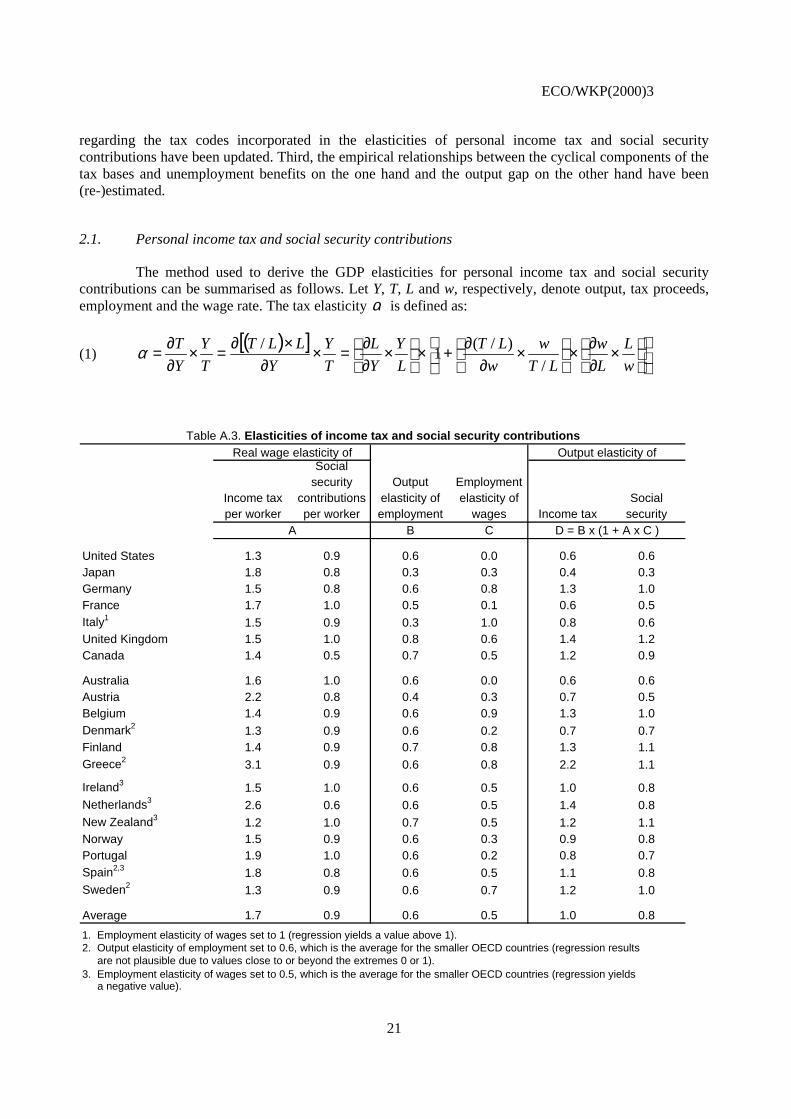
2.1. Personal income tax and social security contributions

The method used to derive the GDP elasticities for personal income tax and social securitycontributions can be summarised as follows. Let Y, T, L and w, respectively, denote output, tax proceeds,employment and the wage rate. The tax elasticity α is defined as:

(1)( )[ ]

×

∂∂×

×

∂∂+×

×

∂∂=×

∂×∂=×

∂∂=

w

L

L

w

LT

w

w

LT

L

Y

Y

L

T

Y

Y

LLT

T

Y

Y

T

/

)/(1

/α

Table A.3. Elasticities of income tax and social security contributionsReal wage elasticity of Output elasticity of

Income tax per worker

Social security

contributions per worker

Output elasticity of employment

Employment elasticity of

wages Income taxSocial

securityA B C D = B x (1 + A x C )

United States 1.3 0.9 0.6 0.0 0.6 0.6Japan 1.8 0.8 0.3 0.3 0.4 0.3Germany 1.5 0.8 0.6 0.8 1.3 1.0France 1.7 1.0 0.5 0.1 0.6 0.5Italy1 1.5 0.9 0.3 1.0 0.8 0.6United Kingdom 1.5 1.0 0.8 0.6 1.4 1.2Canada 1.4 0.5 0.7 0.5 1.2 0.9

Australia 1.6 1.0 0.6 0.0 0.6 0.6Austria 2.2 0.8 0.4 0.3 0.7 0.5Belgium 1.4 0.9 0.6 0.9 1.3 1.0Denmark2 1.3 0.9 0.6 0.2 0.7 0.7Finland 1.4 0.9 0.7 0.8 1.3 1.1Greece2 3.1 0.9 0.6 0.8 2.2 1.1

Ireland3 1.5 1.0 0.6 0.5 1.0 0.8Netherlands3 2.6 0.6 0.6 0.5 1.4 0.8New Zealand3 1.2 1.0 0.7 0.5 1.2 1.1Norway 1.5 0.9 0.6 0.3 0.9 0.8Portugal 1.9 1.0 0.6 0.2 0.8 0.7Spain2,3 1.8 0.8 0.6 0.5 1.1 0.8Sweden2 1.3 0.9 0.6 0.7 1.2 1.0

Average 1.7 0.9 0.6 0.5 1.0 0.8

1. Employment elasticity of wages set to 1 (regression yields a value above 1).2. Output elasticity of employment set to 0.6, which is the average for the smaller OECD countries (regression results are not plausible due to values close to or beyond the extremes 0 or 1).

a negative value).3. Employment elasticity of wages set to 0.5, which is the average for the smaller OECD countries (regression yields

ECO/WKP(2000)3

22

This equation shows that the tax elasticity can be broken down into two sub-elasticities: one todetermine variations in the number of wage earners, and one to determine variations in the tax bill perwage earner. The first term at the right hand side represents the output elasticity of employment, whichserves to capture the impact of cyclical variations in employment on tax proceeds, assuming a given taxyield per worker. This sub-elasticity is typically smaller than 1 due to “Okun’s law” that predicts thatvariations in output are to some extent absorbed by variations in labour productivity. The tax yield perworker, in turn, also varies with the cycle, which is captured by the last term in square brackets. This termprovides a further breakdown into the impact of changes in the wage rate on the tax proceeds per worker(due to tax progressivity) and the employment elasticity of the wage rate. The latter should be interpretedas the “Phillips curve” effect on wages. This calculation is done for each of the 20 countries for which therelevant information is available, and is summarised in Table A.3. The first two columns, marked A, showthe wage elasticity of the tax or social contribution yield per worker. These elasticities are calculated as theratio of the marginal and average rates for an “average” household based on the 1996 tax codes, using thesame methodology as in Giorno et al. (1995). The columns marked B and C in Table A.1 present theoutput elasticities of employment and employment elasticities of wages, respectively, based on theeconometric estimates listed in Tables A.4 and A.5. The columns marked D show the result of thecalculation using equation (1) above.

a2 (t) Adjusted R2

United States 0.61 (7.2) 0.81 Japan 0.27 (4.5) 0.50 Germany2 0.62 (5.8) 0.89 France 0.50 (9.8) 0.79 Italy 0.34 (2.6) 0.80 United Kingdom 0.81 (5.7) 0.58 Canada 0.70 (11.0) 0.90

Australia 0.58 (4.0) 0.37 Austria 0.42 (6.0) 0.59 Belgium 0.57 (8.5) 0.74 Denmark 0.19 (1.7) 0.57 Finland 0.71 (8.6) 0.77 Greece -0.06 (-0.3) 0.29

Ireland 0.58 (7.5) 0.71 Netherlands 0.64 (3.9) 0.89 New Zealand 0.74 (4.0) 0.37 Norway 0.64 (3.9) 0.46 Portugal 0.59 (3.6) 0.80 Spain 1.32 (17.9) 0.93 Sweden 0.89 (6.0) 0.84

1. Estimation period: 1985-1998, semi-annual data. Constant term and time trend are not shown. Potential employment is calculated as (1-NAWRU)xLs*, where NAWRU is the non-accelerating wage rate of unemployment and Ls* is trend labour supply.2. Contains dummy variables to capture re-unification.

Table A.4. Estimated short-run output elasticities of employment

Equation: log (L/L*) = a0 + a1 TIME + a2 log (Y/Y*) where L, L*, Y and Y*

are actual and potential employment and output, respectively;1

ECO/WKP(2000)3

23

b2 (t) Adjusted R2

United States 0.02 (0.1) 0.64 Japan 0.34 (1.5) 0.91 Germany2 0.76 (8.0) 0.92 France2 0.08 (0.5) 0.95 Italy2 1.34 (3.7) 0.88 United Kingdom 0.59 (4.4) 0.65 Canada 0.46 (3.4) 0.31

Australia 0.04 (0.2) 0.66 Austria3 0.34 (1.7) 0.94 Belgium 0.90 (2.7) 0.43 Denmark 0.15 (0.8) 0.01 Finland 0.82 (10.9) 0.95 Greece3 0.81 (1.1) 0.46

Ireland -0.19 (-0.9) 0.91 Netherlands -0.11 (-0.0) 0.96 New Zealand -0.17 (-1.0) 0.72 Norway 0.26 (3.4) 0.32 Portugal4 0.15 (0.5) 0.13 Spain -0.56 (-3.6) 0.72 Sweden 0.69 (5.2) 0.81

1. Estimation period: 1985-1998, semi-annual data. Constant term and time trend are not shown.2. Contains dummy variables.3. Contains an additional quadratic time trend variable.4. Equation reads: d log w = b1 + b2 d log L.

Table A.5. Estimated short-run employment elasticities of real wages

Equation: log (wL*/Y*) = b0 + b1 TIME + b2 log (L/L*) where w = real wage,

L* = potential employment, and Y* = potential output1

2.2. Corporate income tax

The elasticity for the corporate income tax is based on the assumption that the tax rate is strictlyproportional, such that cyclical variations in the tax yield correspond to fluctuations in the tax base,i.e. corporate income. If Z denotes corporate income, the corporate tax elasticity can be broken down asfollows:

(2)( )

Z

Y

w

L

L

w

L

Y

Y

L

Y

Z

Z

Y

Y

wLY

Z

Y

Y

Z

T

Y

Y

T ×

×

∂∂+×

×

∂∂×

−−=×

∂−∂=×

∂∂=×

∂∂= 111α

The proportionality assumption implies that the tax elasticity is equal to the elasticity of the taxbase (profits) with respect to output. The latter, in turn, is a function of the elasticity of the wage bill withrespect to output, with the opposite sign. The elasticity of the wage bill, finally, comprises two sub-elasticities with respect to output, one for employment and one for wages, as shown in the right-hand sideof the formula above. As can be checked easily, the overall elasticity α is equal to unity in case the outputelasticity of employment is equal to 1 and the employment elasticity of real wages equal to 0: in that(extreme) case the wage bill and profits both vary in proportion to output. In practice variations in

ECO/WKP(2000)3

24

employment are less volatile than variations in output while wages show a cyclical pattern, therefore αshould differ from 1 and is most likely larger than 1. Table A.6 shows the result of the calculations. Thefirst column A contains the average profit shares in national income (Z/Y) over the cycle, column B theoutput elasticities of employment and column C the employment elasticities of wages. Note that columns Band C correspond to columns B and C in Table A.3. Column D, finally, combines the components into thereduced form output elasticity of corporate tax, using equation (2) above.

Table A.6. Elasticities of corporate tax

Profit share in GDP

Output elasticity of employment

Employment elasticity of

wages Output elasticity of corporate tax

A B CD = {1 - (1 - A) x B x (1 + C)}

A

United States 30.8% 0.6 0.0 1.8

Japan 37.4% 0.3 0.3 2.1

Germany 33.8% 0.6 0.8 0.8

France 35.2% 0.5 0.1 1.8

Italy 46.7% 0.3 1.0 1.4

United Kingdom 30.6% 0.8 0.6 0.6

Canada 31.0% 0.7 0.5 1.0

Australia 39.8% 0.6 0.0 1.6

Austria 33.9% 0.4 0.3 1.9

Belgium 37.8% 0.6 0.9 0.9

Denmark 32.7% 0.6 0.2 1.6

Finland 34.7% 0.7 0.8 0.7

Greece 56.2% 0.6 0.8 0.9

Ireland 43.5% 0.6 0.5 1.2

Netherlands 37.9% 0.6 0.5 1.1

New Zealand 42.4% 0.7 0.5 0.9

Norway 40.1% 0.6 0.3 1.3

Portugal 41.9% 0.6 0.2 1.4

Spain 44.2% 0.6 0.5 1.1

Sweden 29.8% 0.6 0.7 0.9

Average 38.0% 0.6 0.5 1.3

2.3. Current primary expenditure

Current primary expenditure (G) of general government is assumed to fluctuate in proportionwith unemployment-related expenditure. So, if U is unemployment, UB unemployment benefits and Ls

labour supply, the appropriate formula reads:

ECO/WKP(2000)3

25

(3)

−

×

∂∂−×

×

∂∂×

−=

=

×

∂∂×

∂∂−∂×

=

×

∂∂×

=

×

∂∂×

=×

∂∂=

11ss

s

s

L

U

L

L

L

L

L

Y

Y

L

G

UB

U

Y

Y

L

L

LL

G

UB

U

Y

Y

U

G

UB

UB

Y

Y

UB

G

UB

G

Y

Y

Gβ

It is assumed that unemployment-related expenditure is strictly proportional to unemployment;unemployment benefit rates are seen to be independent of the cycle. Variations in unemployment, in turn,are broken down into two components, capturing variations in employment (the second term in parenthesesat the right hand side) and in the labour force (the last term in brackets). The latter term also contains thelevel of the structural unemployment rate. Note that the expected sign of this elasticity is negative: acyclical upswing in output should lower unemployment-related expenditure and vice versa. Note also thatif the labour force does not react to the cycle, the elasticity collapses into a simple expression containingonly the output elasticity of employment, appropriately weighted by the share of unemployment-relatedexpenditure in total current primary expenditure. The results of the calculations are shown in Table A.7.

Table A.7. Elasticities of current primary expenditure

Output elasticity of employment

Employment elasticity of

labour supply

Trend unemploy-ment rate

Share of unemploy-

ment related in total current primary

expenditure

Output elasticity of unemployment related

expenditure

Output elasticity of

current primary

expenditure

A B C D E = - A x {(1 - B)/C -1} F = D x E

United States 0.6 0.3 5.7% 1.4% -7.0 -0.1

Japan 0.3 0.5 2.7% 2.0% -4.7 -0.1

Germany 0.6 0.8 8.7% 8.6% -0.8 -0.1

France10.5 0.0 10.0% 6.7% -4.5 -0.3

Italy 0.3 0.2 9.5% 5.2% -2.5 -0.1

United Kingdom 0.8 0.3 8.4% 3.9% -5.5 -0.2

Canada 0.7 0.2 9.3% 4.4% -5.0 -0.2

Australia 0.6 0.2 9.0% 6.0% -4.4 -0.3

Austria 0.4 0.8 5.5% 4.0% -1.2 0.0

Belgium1 0.6 0.0 11.3% 9.4% -4.4 -0.4

Denmark10.6 0.0 9.9% 11.9% -5.6 -0.7

Finland 0.7 0.1 10.4% 8.5% -5.2 -0.4

Greece 0.6 1.0 8.9% 2.9% 0.6 0.0

Ireland 0.6 0.3 13.0% 13.9% -2.7 -0.4

Netherlands 0.6 0.2 6.3% 12.7% -7.7 -1.0

New Zealand 0.7 0.3 7.2% 5.7% -6.7 -0.4

Norway 0.6 0.5 4.9% 3.5% -6.1 -0.2

Portugal 0.6 0.5 5.7% 4.8% -4.2 -0.2

Spain 0.6 0.1 20.2% 6.8% -2.1 -0.1

Sweden 0.6 0.4 4.6% 7.8% -7.0 -0.5

Average 0.6 0.3 8.6% 6.5% -4.3 -0.3

1. Employment elasticity of labour supply set to 0 (regression yields a negative value).

ECO/WKP(2000)3

26

Columns A and B contain the output elasticities of employment and employment elasticities of the labourforce, respectively. The “trend” unemployment rate (NAWRU) and the share of unemployment-relatedexpenditure in total current primary expenditure are shown in columns C and D, respectively. Column Eshows the output elasticity of unemployment-related expenditure, which is multiplied by the share ofunemployment-related expenditure in total current primary expenditure in column F to obtain the overallelasticity β. The estimated equations on which the employment elasticities of labour supply are based areshown in Table A.8. In cases where negative values were found the elasticities have been set to 0.

c2 (t) Adjusted R2

United States 0.29 (3.7) 0.92

Japan 0.50 (7.4) 0.90

Germany2 0.80 (9.7) 0.90

France -0.11 (-2.1) 0.97

Italy 0.22 (1.7) 0.62

United Kingdom 0.30 (8.2) 0.94

Canada 0.24 (8.9) 0.97

Australia 0.23 (3.3) 0.32

Austria 0.79 (19.1) 0.97

Belgium -0.13 (-1.2) 0.47

Denmark -0.16 (-0.9) 0.58

Finland 0.07 (1.8) 0.93

Greece 1.05 (10.4) 0.82

Ireland 0.26 (2.4) 0.93

Netherlands 0.18 (1.7) 0.85

New Zealand 0.28 (6.5) 0.65

Norway 0.49 (12.5) 0.88

Portugal3 0.54 (5.9) 0.93

Spain 0.10 (1.8) 0.07

Sweden 0.42 (11.9) 0.90

1. Estimation period: 1985-1998, semi-annual data. Constant term and time trend are not shown.2. Contains dummies.3. Equation reads: d log Ls = c1 + c2 d log L.

Table A.8. Estimated short-run employment elasticities of the labour force

Equation: log (Ls/L*) = c0 + c1 TIME + c2 log (L/L*) where Ls = labour suply,

L and L* are actual and potential employment1

2.4. Indirect tax

To calculate the elasticity for indirect tax the assumption has been made that the relevant tax basefluctuates in proportion with private consumption. Based on this assumption, the elasticity for indirect taxcorresponds to the output elasticity of consumption, which is shown in Table A.1. These elasticities arebased on estimation results that are summarised in Table A.9.

ECO/WKP(2000)3

27

d2 (t) Adjusted R2

United States 0.94 (12.6) 0.88 Japan 0.46 (7.5) 0.79 Germany 0.95 (3.6) 0.65 France 0.68 (7.1) 0.73 Italy 1.36 (7.7) 0.74 United Kingdom 1.10 (9.0) 0.77 Canada 0.73 (10.4) 0.85

Australia 0.40 (3.5) 0.43 Austria 0.53 (2.0) 0.54 Belgium 0.89 (8.9) 0.79 Denmark 1.59 (15.0) 0.91 Finland 0.90 (11.6) 0.91 Greece 0.75 (3.1) 0.57

Ireland 0.47 (2.5) 0.91 Netherlands 0.74 (4.3) 0.52 New Zealand 1.15 (4.3) 0.26 Norway 1.58 (11.6) 0.83 Portugal 0.64 (5.7) 0.74 Spain 1.20 (12.5) 0.89 Sweden 0.86 (5.3) 0.88

1. Estimation period: 1985-1998, semi-annual data. Constant term and time trend are not shown. Estimated with 2SLS method to correct for simultaneity.

Table A.9. Estimated short-run output elasticities of real

private consumption

Equation: log (C/Y*) = d0 + d1 TIME + d2 log (Y/Y*) where C = private

consumption, Y and Y* are actual and potential output1

3. Sensitivity analysis

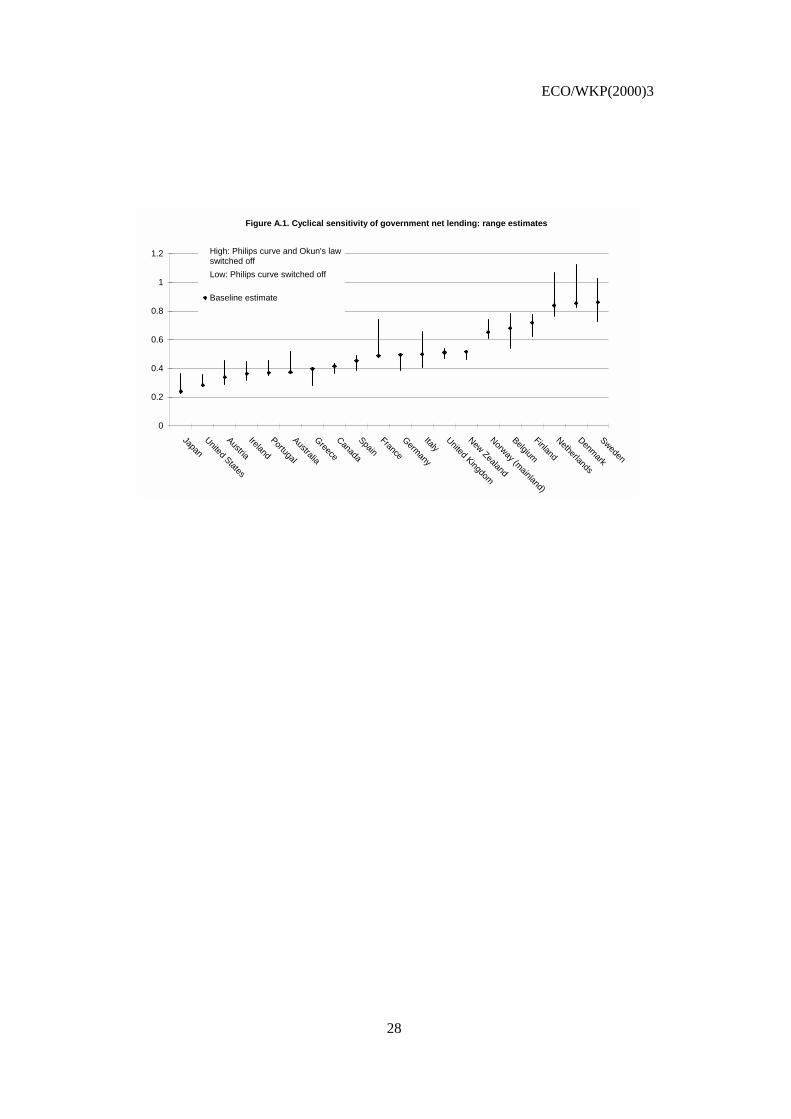
The above methodology assumes that employment varies less than proportionally with output(Okun’s law), while wages display some sensitivity to cyclical variations in employment (Philips curve). Itmay be useful to quantify the impact of these assumptions on the estimated cyclical sensitivity ofgovernment net lending as a share of GDP. The last column of TableA.1 provides such estimates for thebaseline case, the average of which for the countries considered is 0.5. Two alternative sets of semi-elasticities have been calculated. In the first alternative set, the Phillips curve has been switched off, suchthat wages are assumed not to vary with employment over the cycle (the short-run employment elasticityof wages is zero), hence tax progressivity does not play any role. As a result the semi-elasticities fall by onaverage 0.05, to 0.45, with some marked variation across countries (Figure A.1). In Sweden, for example,the semi-elasticity drops from around 0.8 to 0.6, whereas several other countries display virtually nochange. In the second alternative, Okun’s law has been switched off in addition. Hence employment variesproportionally with output (the output elasticity of employment is equal to 1), whereas wages are constant.Under this assumption the personal income and social security tax bases as well as unemployment-relatedexpenditure vary more sharply than in the baseline case, whereas corporate taxes vary less sharply. Giventhe small share of corporate taxes, however, the semi-elasticities increase, as is shown in Figure A.1. Whileon average the semi-elasticities rise from 0.5 to 0.6, the variation across countries is again significant, withthe biggest increases found in France, Denmark and the Netherlands.

ECO/WKP(2000)3

28

Figure A.1. Cyclical sensitivity of government net lending: range estimates

0

0.2

0.4

0.6

0.8

1

1.2

Japan

UnitedStates

Austria

Ireland

Portugal

Australia

Greece

Canada

SpainFrance

Germany

ItalyUnited

Kingdom

NewZealand

Norway (mainland)

Belgium

Finland

Netherlands

Denmark

Sweden

High: Philips curve and Okun's lawswitched off

Low: Philips curve switched off

Baseline estimate

ECO/WKP(2000)3

29

REFERENCES

Asdrubali, A., B.E. Sorensen and O. Yosha (1996), “Channels of interstate risk sharing: United States1963-1990”, Quarterly Journal of Economics, Vol. 111, pp. 1081-1110.

Bismut, C.J. (1995), Trends and cycles in government revenues in France, IMF (mimeo).

Buti, M. and A. Sapir, eds. (1998), Economic Policy in EMU -- A study by the European CommissionsServices, Oxford University Press.

Dalsgaard, T. and A. DeSerres (1999), Estimating prudent budgetary margins to comply with the Stabilityand Growth Pact: a simulated SVAR approach, OECD Economics Department Working PaperNo. 216.

Elmeskov, J. and M. MacFarlan (1993), “Unemployment persistence”, OECD Economic Studies, No. 21,pp. 59-88.

Giavazzi, F. and M. Pagano (1990), Can severe fiscal contractions be expansionary? Tales of two smallEuropean countries, CEPR, Discussion Papers No. 147, London.

Giavazzi, F. and M. Pagano (1995), Non-Keynesian effects of fiscal policy changes: international evidenceand the Swedish experience, CEPR Discussion Paper No. 1284, London.

Giorno, C., P. Richardson, D. Roseveare and P. van den Noord (1995), “Potential output, output gaps andstructural budget balances”, OECD Economic Studies, No. 24, pp. 167-209.

Leibfritz, W., D. Roseveare and P. van den Noord (1994), Fiscal policy, government debt and economicperformance, OECD Economics Department Working Papers, No. 144.

Martinot, B. (1999), Pacte de stabilité et efficacité de la politique budgétaire, Ministère des Finances, Paris(mimeo).

OECD (1999), Implementing the OECD Jobs Strategy : Assessing Performance and Policy, Paris.

Orr, A., M. Edey and M. Kennedy (1995), “Real long-term interest rates: the evidence from pooled-time-series”, OECD Economic Studies, No. 25, pp. 75-107.

Sutherland, A. (1997), “Fiscal crises and aggregate demand: can high public debt reverse the effects offiscal policy?”, Journal of Public Economics, No. 63, pp. 147-162.

ECO/WKP(2000)3

30

ECONOMICS DEPARTMENTWORKING PAPERS

229. Enhancing environmentally sustainable growth in Finland(January 2000) Ann Vourc’h and Miguel Jimenez

228. Finance and growth: Some theoretical considerations, and a review of the empirical literature(January 2000) Kotaro Tsuru

227. What the yield curves say about inflation: Does it change over time?(December 1999) Sebastian T. Schich

226. Summary Indicators of Product Market Regulation with an Extension to Employment Protection Legislation(December 1999) Giuseppe Nicoletti, Stefano Scarpetta and Olivier Boylaud

225. Some Issues Related to the Equity-Efficiency Trade-Off in the Sweden Tax and Transfer System(December 1999) Giuseppe Nicoletti, Stefano Scarpetta and Olivier Boylaud

224. The Economic Effects of Employment-Conditional Income Support Schemes for the Low-Paid : An Illustrationfrom a CGE Model Applied to Four OECD Countries(October 1999) Andrea Bassanini, Jørn Henrik Rasmussen and Stefano Scarpetta

223. The Use of Financial Market Indicators by Monetary Authorities(September 1999) Paul Mylonas and Sebasian Schich

222. Tax Reform in Switzerland(August 1999) David Carey, Kathryn Gordon and Philippe Thalman

221. Trends in Market Openness(August 1999) Jonathan Coppel and Martine Durand

220. Technology Upgrading with Learning Cost : A Solution for Two “Productivity Puzzles”(July 1999) Sanghoon Ahn

219. Testing for a Common OECD Phillips Curve(July 1999) Dave Turner and Elena Seghezza

218. Sustainable Economic Growth: Natural Resources and the Environment(July 1999) Paul van den Noord and Ann Vourc’h

217. Coping with Population Ageing in Australia(July 1999) David Carey

216. Estimating Prudent Budgetary Margins for 11 EU Countries : A Simulated SVAR Model Approach(July 1999) Thomas Dalsgaard and Alain de Serres

215. The Problems and Prospects Faced by Pay-As-You-Go Pension Systems : A Case Study of Greece(June 1999) Paul Mylonas and Christine de la Maisonneuve

214. Greek Public Enterprises : Challenges for Reform(May 1999) Paul Mylonas and Isabelle Joumard

213. The Levels and Cyclical Behaviour of Mark-Ups Across Countries and Market Structures(May 1999) Joaquim Oliveira Martins and Stefano Scarpetta

ECO/WKP(2000)3

31

212. Poverty Dynamics in Four OECD Countries(April 1999) Pablo Antolín, Thai-Thanh Dang and Howard OxleyAssisted by Ross Finnie and Roger Sceviour

211. The Recent Experience with Capital Flows to Emerging Market Economies(February 1999) Sveinbjörn Blöndal and Hans Christiansen

210. Foreign Portfolio Investors Before and During a Crisis(February 1999) Woochan Kim and Shang-Jin Wei

209. Towards More Efficient Government : Reforming Federal Fiscal Relations in Germany(February 1999) Eckhard Wurzel

208. Stock Market Fluctuations and Consumption Behaviour : Some Recent Evidence(December 1998) Laurence Boone, Claude Giorno and Pete Richardson

207. Microeconometric analysis of the retirement decision: The Netherlands(June 1998) Maarten Lindeboom

206. Microeconometric analysis of the retirement decision: United Kingdom(June 1998) Raffaele Miniaci and Elena Stancanelli

205. Microeconometric analysis of the retirement decision: Italy(June 1998) Raffaele Miniaci

204. Microeconometric analysis of the retirement decision: Germany(June 1998) Pablo Antolin and Stefano Scarpetta

203. Microeconometric analysis of the retirement decision: United States(June 1998) Joseph Quinn, Richard Burkhauser, Kevin Cahill and Robert Weathers

202. The retirement decision in OECD countries(June 1998) Sveinbjörn Blöndal and Stefano Scarpetta

201. The macroeconomic effects of pension reforms in the context of ageing populations:overlapping generations model simulations for seven OECD countries(June 1998) Ketil Hviding and Marcel Mérette

200. The macroeconomics of ageing, pensions and savings: a survey(June 1998) Richard Kohl and Paul O’Brien

199. Marginal Effective Tax Rates on Physical, Human and R&D Capital(May 1998) Kathryn Gordon and Harry Tchilinguirian

198. The Norwegian Health Care System(May 1998) Paul van den Noord, Terje Hagen and Tor Iversen

197. APEC Trade Liberalisation : Its Implications(May 1998) Seunghee Han and Inkyo Cheong