the shape synthesis of antenna decoupling surfaces
TRANSCRIPT

The Shape Synthesis of Antenna Decoupling
Surfaces
Mohammed Raei
Thesis submitted to the University of Ottawa
in partial Fulfillment of the requirements for the
Master of Applied Science
in Electrical & Computer Engineering
Ottawa-Carleton Institute for Electrical and Computer Engineering
School of Electrical Engineering and Computer Science
Faculty of Engineering
University of Ottawa
© Mohammed Raei, Ottawa, Canada, 2021

ii
ABSTRACT
Although multi-element antenna (MEA) systems are already used in some modern wireless
communication systems, the issue of mutual coupling between elements remains a challenge
during MEA system design. Indeed, communications engineers continue to bemoan the fact that
that the antenna elements are often still designed with such coupling as an afterthought. Thus,
some authors have used the decoupling surface (DS) idea, whereby a separate DS is added to the
MEA systems to reduce the above coupling. Whereas a DS may indeed lower the coupling levels
between the elements of a given MEA system, it usually changes the other performance parameters
as well, and in an undesirable way. Thus, this design route is a complicated one that is not easily
effected. In this thesis we propose, for the first time, a new design process for MEA systems based
on shape synthesis. The MEA system performance indicators are combined into an objective that
sets the goal of the shape synthesis procedure. The application of the proposed design process is
illustrated for three different geometrical arrangements of patch antennas and decoupling surfaces.
This confirms the efficacy of the new design method.
Keywords: multi-element antennas, MIMO, mutual coupling, decoupling, isolation, total active
reflection coefficient (TARC), envelope correlation coefficient (ECC).

iii
Acknowledgements
I am grateful to my supervisor Dr. Derek McNamara for his counsel and support while
completing this thesis and for allowing me to liberally use sample review material for Chapter 2
from the notes of the various courses he presents at the University of Ottawa. Thank you for the
invaluable information you have taught me throughout my undergraduate and graduate studies.
I would also like to thank my first teacher, my mother Alia, for teaching me about the value of
education. I am also thankful to my father, Najib, for always believing in me and pushing me to
accomplish great things. My gratitude is extended to my three sisters Beesan, Nour and Saba and
my fiancée Maryam for always being there for me.

iv
Table of Contents
Chapter 1 Introduction .................................................................................................................... 1
Introductory Comments.................................................................................................... 1
Multi-Element Antenna Systems ..................................................................................... 2
Coupling in Multi-Element Antenna Systems ................................................................. 3
Multi-Element Antenna System Design ........................................................................... 4
Overview of the Thesis .................................................................................................... 5
Chapter 2 Review of Key Background Concepts & Techniques .................................................... 7
Introduction ...................................................................................................................... 7
Clarification of the Meaning of “Shape Synthesis” ......................................................... 7
Multi-Element Antenna System Figures of Merit ............................................................ 8
Introductory Comments ................................................................................................. 8
Far-Zone Fields & Radiation Patterns ........................................................................... 8
Fractional Bandwidth ................................................................................................... 14
Input Reflection Coefficient of an Isolated Antenna ................................................... 15
Radiation Efficiency .................................................................................................... 16
Total Active Reflection Coefficient (TARC) .............................................................. 16
Envelope Correlation Coefficient ................................................................................ 18
The Need for Low Mutual Coupling Between MIMO Antennas ................................ 27
Technical Definition of Mutual Coupling.................................................................... 28
Inter-Element Coupling Requirements in MIMO Systems ....................................... 29
Radiation Pattern Requirement for MIMO Antennas ................................................ 31
Existing Coupling Reduction Methods in MEA Systems .............................................. 31
Preliminary Notes ........................................................................................................ 31

v
Eigenmode Decomposition Schemes ........................................................................... 31
Inserted Component Schemes ...................................................................................... 33
Coupled Resonator Schemes ........................................................................................ 36
Decoupling Surface Schemes ...................................................................................... 41
Existing Use of Optimization in MIMO Antenna Design ........................................... 45
Computational Approach Harnessed in the Thesis for Shape Synthesis ....................... 52
Conclusions .................................................................................................................... 53
Chapter 3 The Shape Synthesis of Coplanar Decoupling Surfaces .............................................. 54
Goals............................................................................................................................... 54
Objective Functions........................................................................................................ 54
The Shape Synthesis Process ......................................................................................... 58
Linearly Polarized Microstrip Patches: H-Plane Coupling ............................................ 61
Goals ............................................................................................................................ 61
Single Probe-fed Microstrip Patch ............................................................................... 62
MEA consisting of two microstrip patch antennas ...................................................... 63
Insertion of an unshaped decoupling surface ............................................................... 66
Application of Shape Synthesis ................................................................................... 69
Linearly Polarized Microstrip Patches: E-Plane Coupling ............................................ 77
Preamble ...................................................................................................................... 77
Single Microstrip Patch Reference .............................................................................. 77
MEA Consisting of Two Patch Antennas: E-Plane Alignment ................................... 80
MEA Consisting of Two Patch Antennas and an (Unshaped) Decoupling Surface .... 83
Patch Antenna Polarization ............................................................................................ 94
Concluding Remarks ...................................................................................................... 96
Chapter 4 The Shape Synthesis of Non-Coplanar Decoupling Surfaces ...................................... 97

vi
Preliminary Remarks ...................................................................................................... 97
Single Probe-Fed Microstrip Patch ................................................................................ 97
MEA System Consisting of Four Patch Antennas ....................................................... 100
The 4-Element MEA & an Unshaped Decoupling Surface ......................................... 108
Objective Function Used in the Shape Synthesis Process............................................ 112
Shape Synthesis Results ............................................................................................... 115
Concluding Remarks .................................................................................................... 122
Chapter 5 General Conclusions .................................................................................................. 123
Contributions ................................................................................................................ 123
Possible Future Work ................................................................................................... 125
Appendix A: Multiple-Input Multiple-output (MIMO) Systems................................................ 126
A.1 MIMO Diversity Techniques .................................................................................... 126
A.2 Massive MIMO ......................................................................................................... 127

vii
Table of Figures
Figure 2.3-1: Systems view of an antenna (Diagram courtesy of D.A.McNamara) ....................... 8
Figure 2.3-2: Spherical Coordinates with antenna at the center (Diagram courtesy of
D.A.McNamara) ........................................................................................................................... 13
Figure 2.3-3: Two closely spaced dipole antennas ....................................................................... 22
Figure 2.3-4: ECC plots for dipole antennas ................................................................................ 23
Figure 2.3-5: Two dipole antenna and a passive wire. ................................................................. 24
Figure 2.3-6: ECC results for two dipole antennas and a passive wire ........................................ 24
Figure 2.3-7: Two patch antennas on a lossy substrate with 휀𝑟 = 0.04 and 𝑡𝑎𝑛𝛿 = 0.005. ....... 25
Figure 2.3-8: ECC curves for the two patch antennas shown in Figure 2.3-7. ............................. 25
Figure 2.3-9: ECC curves for the two patch antennas shown in Figure 2.3-7 but with tan𝛿 = 0.01.
....................................................................................................................................................... 26
Figure 2.3-10: ECC curves for the two patch antennas shown in Figure 2.3-7 but with tan𝛿 =
0.025.............................................................................................................................................. 27
Figure 2.3-11: Data throughput versus received power for antennas with different levels of
mutual coupling. Macro-cell on the left and micro-cell on the right. (After [MEI 18]) ............... 30
Figure 2.4-1: Four ports feeding a single multimode antenna [MANT 16] .................................. 32
Figure 2.4-2: Normalized magnitude of the total electric field of first CM vs. chassis geometry
[LI 12] ........................................................................................................................................... 33
Figure 2.4-3: Top view of substrate (left), and (right) bottom view (After [LIU 13]). ................ 34
Figure 2.4-4: S21 Plots: (- . - ) no parasitic stubs, (- - -) only vertical stub, (....) horizontal stub
only, and (____) both stubs (After[ LIU 14]). .............................................................................. 35
Figure 2.4-5: EBG and two patch antennas coupled in E-Plane. (After [YANG 03]) ................. 35
Figure 2.4-6: Measured results of microstrip antennas with and without EBG............................ 36
Figure 2.4-7: PIFA antennas on PCB (After [DIAL 06]) ............................................................. 37
Figure 2.4-8: 2 PIFA's with NL's connected (After [DIAL06]) ................................................... 38
Figure 2.4-9: The S-parameter response before introducing the NL (After [DIAL 06]) .............. 39
Figure 2.4-10: The S-parameter response after introducing the NL (After [DIAL 06]) .............. 39
Figure 2.4-11: Design of two Antennas with NL (After [ZHAN 16]).......................................... 40
Figure 2.4-12: S-parameters with and without NL (After [ZHAN 16]) ....................................... 41

viii
Figure 2.4-13: Quasi-Yagi antennas and antenna decoupling surface (After [WEI 16]) ............. 42
Figure 2.4-14: Effect of the DS on the S-parameters ( After [WEI 16]) ...................................... 42
Figure 2.4-15: (a) Antennas and DS (b) Cross dipole arrangement (after [WU 17]) ................... 43
Figure 2.4-16: Simulated and Measured S-parameters (After [WU 17]) ..................................... 44
Figure 2.4-17: Efficiency of the antennas before and after optimization (After [KARL 09])...... 46
Figure 2.4-18: Diversity Gain before and after optimization (After [KARL 09]) ........................ 46
Figure 2.4-19: Monopole parameters to be optimized, (b) 3D view of the monopole antenna
(After [BEKA 16]) ........................................................................................................................ 47
Figure 2.4-20: S11 simulation results for initial (- -) and optimized (___) antennas (After [BEKA
16]) ................................................................................................................................................ 47
Figure 2.4-21: Arrangement of the optimized antennas (After [BEKA 16]) ................................ 48
Figure 2.4-22: Simulated S-parameters of MIMO antennas: S11 (___), S22 (- -) and S12 ( ... ) (After
[BEKA 16]) ................................................................................................................................... 48
Figure 2.4-23: Initial antenna arrangement "pre-optimization" (After [DERN 11]) .................... 49
Figure 2.4-24: Different results of the simulation. ....................................................................... 50
Figure 2.4-25: Simulated S-parameter of the optimized design (After [DERN 11]).................... 51
Figure 2.4-26: Simulated radiation efficiencies, average efficiency, and MIMO efficiency (After
[DERN 11]). .................................................................................................................................. 51
Figure 3.2-1: An example of S-parameter mask function............................................................. 55
Figure 3.3-1: Flowchart describing the HyperStudy GA operation .............................................. 60
Figure 3.4-1: Unshaped MEA (mother structure) ......................................................................... 61
Figure 3.4-2: Dimensions of a single probe-fed microstrip patch antenna ................................... 62
Figure 3.4-3: Computed reflection coefficient for the single patch antenna in Figure 3.4-2 ....... 62
Figure 3.4-4: Computed total directivity patterns for a single antenna at 5.7 GHz. The pattern
coordinate system is shown in Fig 3.4-1, and defines angle 𝝓. .................................................... 63
Figure 3.4-5:Dimensions of MEA design ..................................................................................... 64
Figure 3.4-6: Computed S-parameter plot for MEA ..................................................................... 65
Figure 3.4-7: Surface current density for MEA at 5.7 GHz .......................................................... 65
Figure 3.4-8: Computed total directivity patterns of antenna 1, when antenna 2 is terminated in a
matched load, at 5.7 GHz. ............................................................................................................. 66
Figure 3.4-9: Dimensions of MEA after introducing the DS........................................................ 67

ix
Figure 3.4-10: Computed S-parameter plots after the DS is introduced....................................... 67
Figure 3.4-11: Surface current density of MEA with DS, with antenna 1 excited and antenna 2
terminated with a matched load, at 5.7 GHz. ................................................................................ 68
Figure 3.4-12: Computed total directivity patterns at 5.7 GHz, when antenna 1 is excited, with
the unshaped DS present. .............................................................................................................. 69
Figure 3.4-13: Selected masks for S11 and S12 .............................................................................. 71
Figure 3.4-14: Symmetry enforced on the pixelated shape of the MEA to be shaped. ................ 72
Figure 3.4-15: Objective function values during the shape synthesis process ............................. 73
Figure 3.4-16: Shape Synthesized MEA ....................................................................................... 73
Figure 3.4-17: Simulated S-parameters of shaped MEA .............................................................. 74
Figure 3.4-18: Surface current density for shaped H-plane model ............................................... 75
Figure 3.4-19: Computed total directivity pattern of the shaped MEA. ....................................... 75
Figure 3.4-20: Simulated radiation efficiency before and after shaping ...................................... 76
Figure 3.5-1:Dimensions of the unshaped MEA arrangement (E-plane coupling) that will form
the starting shape for the shape synthesis application. ................................................................. 78
Figure 3.5-2: Computed reflection coefficient of the single isolated patch antenna .................... 79
Figure 3.5-3: Computed total directivity radiation pattern of the single patch antenna in the two
principal planes. The frequency is 5.55 GHz. ............................................................................... 79
Figure 3.5-4: Computed S-parameters of the MEA (two patches without a DS). ........................ 80
Figure 3.5-5: Surface current density on the MEA(two patches and no DS) when port#1 is driven
and port#2 terminated. The frequency is 5.55 GHz. ..................................................................... 81
Figure 3.5-6: Computed principal plane total directivity patterns of the MEA (two patches and no
DS) when port#1 is driven and port#2 terminated. The frequency is 5.55 GHz. ......................... 81
Figure 3.5-7: ECC for the MEA (two patches and no DS). .......................................................... 82
Figure 3.5-8: Computed TARC for the MEA (two patches and no DS). ..................................... 83
Figure 3.5-9: Computed S-parameters of the MEA consisting of two patches and the unshaped
DS. ................................................................................................................................................ 84
Figure 3.5-10: Surface current density on the MEA consisting of two patches and the unshaped
DS when port#1 is driven and port#2 terminated. The frequency is 5.55 GHz. ........................... 85
Figure 3.5-11: Computed total directivity principal plane patterns of the MEA consisting of two
patches and the unshaped DS. The frequency is 5.55 GHz .......................................................... 85

x
Figure 3.5-12: Computed ECC for the MEA consisting of two patches and the unshaped DS. .. 86
Figure 3.5-13: Starting Structure of E-Plane coupled MEA ......................................................... 86
Figure 3.5-14: Objective function value during the shape optimization of the MEA consisting of
two patches and DS ....................................................................................................................... 89
Figure 3.5-15: The MEA consisting of two patches and a DS after the shaping is completed .... 89
Figure 3.5-16: Computed S-parameter plots for the shaped MEA consisting of two patches and a
DS. ................................................................................................................................................ 90
Figure 3.5-17: Surface current density on the shaped MEA consisting of two patches and a DS,
when port#1 is driven and port#2 terminated. The frequency is 5.55 GHz. ................................. 91
Figure 3.5-18: Computed total directivity principal plane patterns on the shaped MEA consisting
of two patches and a DS when port#1 is driven and port#2 terminated. The frequency is 5.55
GHz. .............................................................................................................................................. 92
Figure 3.5-19: Computed ECC for the shaped MEA consisting of two patches and a shaped DS.
....................................................................................................................................................... 93
Figure 3.5-20: TARC curves for the shaped MEA consisting of two patches and a DS. ............. 93
Figure 3.5-21: Simulated radiation efficiency plots before and after shaping two patches and DS
....................................................................................................................................................... 94
Figure 3.6-1: Computed cross-polarization directivity components in the farfield for two
antennas and DS before and after shaping (H-plane case) ........................................................... 95
Figure 3.6-2: Computed cross-polarization directivity components in the farfield for two
antennas and DS before and after shaping (E-plane case) ............................................................ 95
Figure 4.2-1: Dimensions of a single patch antenna which will be used in MEA ........................ 98
Figure 4.2-2: Computed reflection coefficient of the single isolated patch antenna .................... 99
Figure 4.2-3: Computed total directivity of the isolated patch antenna at f=5.7 GHz. ................. 99
Figure 4.3-1: Dimension of MEA consisting of four patch antennas ......................................... 100
Figure 4.3-2: Computed S-parameters of the MEA (four patches without DS). ........................ 101
Figure 4.3-3: Surface current density on the MEA (four patches and no DS) when port#1 is
driven, and the remaining ports are terminated. The frequency is 5.7 GHz. .............................. 102
Figure 4.3-4: Computed total directivity pattern of the MEA when port#1 is driven and the
remaining ports are terminated. The frequency is 5.7 GHz. ....................................................... 103
Figure 4.3-5: ECC for MEA (four patches no DS) ..................................................................... 104

xi
Figure 4.3-6: TARC of MEA consisting of 4 patch antennas and no DS. These plots are taken
when Antenna #1 and #2 have constant phase, while antenna #3 and #4 have a varying phase. 107
Figure 4.3-7: TARC of MEA consisting of 4 patch antennas and no DS. These plots are taken
when Antenna #1 and #3 have constant phase, while antenna #2 and #4 have a varying phase. 107
Figure 4.3-8: TARC of MEA consisting of 4 patch antennas and no DS. These plots are taken
when Antenna #1 and #4 have constant phase, while antenna #2 and #3 have a varying phase. 108
Figure 4.4-1: Top and Iso view of the MEA after introducing the DS ....................................... 109
Figure 4.4-2: Dimensions of the DS ........................................................................................... 109
Figure 4.4-3: Computed S-parameter plots of the MEA consisting of four patches and the
unshaped DS. .............................................................................................................................. 110
Figure 4.4-4: Computed total directivity pattern of the MEA consisting of four patches and the
unshaped DS, when port#1 is driven and remaining ports are terminated. The frequency is 5.7
GHz ............................................................................................................................................. 111
Figure 4.4-5: Surface current on DS when port#1 is driven and the remaining ports are
terminated. The frequency is 5.7 GHz ........................................................................................ 111
Figure 4.4-6: Surface current on the MEA when port#1 is driven and the remaining ports are
terminated. The frequency is 5.7 GHz. ....................................................................................... 112
Figure 4.5-1: Symmetry is retained after removal of cells in the DS ......................................... 113
Figure 4.5-2: Objective function value during the shape synthesis of the MEA consisting of four
patches and a DS. ........................................................................................................................ 115
Figure 4.6-1: DS after the shaping process ................................................................................. 115
Figure 4.6-2: Computed S-parameter plots of the 4 patch MEA and shaped DS. ...................... 116
Figure 4.6-3: Computed total directivity principal plane patterns of the MEA and shaped DS
when port#1 is driven and the remaining ports are terminated. The frequency is 5.7 GHz ....... 117
Figure 4.6-4: The surface current density on the MEA after the DS has been shaped when port#1
is driven and the remaining ports are terminated. The frequency is 5.7 GHz. ........................... 118
Figure 4.6-5: The surface current density on the shaped DS when port#1 is driven and the
remaining ports are terminated. The frequency is 5.7 GHz. ....................................................... 118
Figure 4.6-6: ECC plots for MEA consisting of four patch antennas without a DS, compared to
adding a shaped DS. .................................................................................................................... 119

xii
Figure 4.6-7:TARC of MEA consisting of 4 patch antennas and shaped DS. These plots are taken
when Antenna #1 and #2 are constant while antenna #3 and #4 have a varying phase.............. 120
Figure 4.6-8:TARC of MEA consisting of 4 patch antennas and shaped DS, taken when antenna
1 and 3 are constant and antenna 2 and 4 are varying phase. ..................................................... 120
Figure 4.6-9: :TARC of MEA consisting of 4 patch antennas and shaped DS Taken when
Antenna #1 and #4 are constant and antennas #2 and #3 are varying phase. ............................. 121
Figure 4.6-10: Simulated radiation efficiency plots before and after shaping DS...................... 121

1
Chapter 1 Introduction
Introductory Comments
Multiple-input multiple-output (MIMO) systems1 have been a topic of great interest in the field
of wireless communications. It has been shown, theoretically and through testing, that MIMO
systems make it possible to exceed the theoretical limit of channel capacity predicted by the
conventional form of the Shannon - Hartley formula. The point of reference here is the
communication channel, when referring to MIMO we refer to multiple signals entering the
communication channel and multiple signals output at the receiver end. The key advantage offered
by such systems is that the increase in capacity that they offer does not come at the expense of
increased consumption of resources such as power and bandwidth. Wireless communication
channels have many impairments. Line-of-sight (LOS) propagation channels suffer from path loss
and interference. With portable wireless user equipment being widely available, robust and reliable
communication in non line-of-sight (NLOS) environments is needed. In addition to suffering from
the LOS impairments mentioned, NLOS communications also suffer from significant fluctuations
of the received signal. In NLOS environments propagating signals are obstructed by manmade or
natural obstacles. This causes the signal to suffer reflection, refraction and diffraction by material
objects (eg. buildings), processes collectively referred to as scattering. The scattering phenomena
cause multiple copies of the same signal to arrive at the receiver; these interfere with each other
constructively or destructively in a random manner [FRAN 08]. Consequently, the power level of
the received signal fluctuates at the receiver and in some instances the received signal becomes
too weak to be retrieved. The received signal is said to be experiencing fading.
Prior to the invention of MIMO, most researchers focused on ways to combat fading in propagation
environments, as multipath fading was the main culprit in causing degradation of the performance
of traditional single input single output (SISO) systems. However, this view of multipath fading
changed in 1996 when it was shown that the use of multi-element antenna (MEA) systems using
multiple element antennas (MEA) for transmission and reception in a Rayleigh fading environment
1 Although such ideas have become familiar, some technical detail on the topic of MIMO systems is provided for
convenience in Appendix A.

2
can result in a linear increase in channel capacity [FOSC 96]. The work presented in [FOSC 96],
combined with the powerful signal processing circuitry available today, made it possible to
implement MIMO.
The use of antenna diversity at the receiver end to decrease the probability of fading had been
known for a long time. Already in the 1930’s, Beverage combined the output of three receiving
antennas in order to increase the signal to noise ratio (SNR) by mitigating the effects of fading
[BEVE 31]. Modern diversity schemes for SISO systems include time diversity and frequency
diversity. In time diversity, the same signal is sent in different time slots, thus reducing the
probability of fading as the channel behavior is expected to change over time. Frequency diversity
is effectively sending the same signal using different frequencies; this is based on the idea that
different frequencies have different scattering characteristics. Modern MIMO systems make use
of fading in order to increase the channel capacity by exciting different independent sub-channels
in the communication channel. Nonetheless, if the communication sub-channels are not
sufficiently uncorrelated or independent, the MIMO system will not function properly as signal
loss could occur.
The channel capacity of a SISO system is mainly affected by the antenna gain. However, that is
not the case when one is designing antennas for MIMO since the system’s capacity is also
dependent on the way the antennas excite the propagation channel [JENS 04]. As such, the cost of
achieving this increased capacity is the necessary development and engineering of more complex
systems. In addition to accounting for “classical” antenna performance parameters such as
radiation patterns, radiation efficiency, and bandwidth, the antenna designer has to design for
MIMO specific performance indicators such as low correlation2. As will be shown in this thesis,
all such requirements can be met simultaneously using shape synthesis.
Multi-Element Antenna Systems
The IEEE defines an array antenna as “an antenna comprised of a number of radiating elements
the inputs (or outputs) of which are combined” [IEEE 13]. Although this definition can be
considered to incorporate what is meant by a multi-element antenna (MEA) system, it will prevent
confusion if we clarify the difference between a “conventional” (multi-element) array antenna and
2 More will be said about this in Section 1.4, and then in much more detail in Section 2.3.

3
what is usually meant by a multi-element antenna system. In an array antenna the elements
typically used in concert, through combination of the element ports via a beamforming network
(BFN), to obtain a single-port antenna with a gain higher that that offered by individual elements.
The entire array is used to receive or transmit the same signal. However, this is not the case in
MEA systems where the elements are designed to operate on independent signals [VAUG 03]. In
an MEA system each element is physically separated from the other elements and has a dedicated
port. Each element can even have distinct characteristics (polarizations, radiation patterns, and so
on).
In addition to being strong candidates for 5G communication applications, MEA systems have
been a topic of interest among radar design engineers. MIMO radars use MEA to transmit and
receive independent waveforms thereby exploiting the system’s diversity. It has been shown that
MIMO radars demonstrate superior performance in terms of resolution, and radar cross section
fluctuation [FISH 04] [XU 07]. Often, antennas meant for radar applications are well spaced,
therefore mitigating the coupling effect does not pose a challenge. Therefore, this thesis will only
focus on the decoupling of the elements in MEA systems used for wireless communications.
Coupling in Multi-Element Antenna Systems
Consider a two-element antenna system (consisting of antennas “1” and “2”), where the
elements are placed near to each other. When antenna “1” transmits a signal, assuming a “good”
antenna design with reasonable port-to-port isolation, most of the signal will be radiated into the
environment. However, some of the signal will be incident on the adjacent transmit antenna. A
portion of this incident field will make its way into the transmission line feed of antenna “2”, and
affect its performance metrics. Similarly, some of this incident field on “2” will be re-scattered off
the structure of antenna “2” and some of this re-scattered field will be incident back on antenna
“1” even though most will be transmitted into the environment. This unintentional scattering
results in mutual coupling between the antennas [ALLE 66] [CHEN 18]. If we extend the above
to an N-element antenna system, we can see that the unwanted coupling into any one element will
be stronger as the signals would scatter from N-1 adjacent antennas. In other words, the mutual
coupling would occur between antennas 1 and 2, 1 and 3, 2 and 3, and so on. The scaling for
mutual coupling in N-element MEA systems is true for both transmitting and receiving modes.
Generally, mutual coupling in MEA systems is a function of the relative spacing of the antennas

4
and the number of antenna elements. Additional factors which affect the mutual coupling include
the relative arrangements of the antennas as well as the relative orientation of the elements [BALA
16].
In this thesis we will consider MEA systems whose elements are microstrip patches. Coupling
between microstrip patch elements occurs due to the excitation of space waves and surface waves
[BALA 16]. Space waves are waves which are radiated into free space (become detached from
the substrate) [BHAT 90] and have an inverse distance decay rate [BALA 16]. The other source
of coupling in microstrip patch elements are surface waves, which are spawned as a result of the
excitation of guided waves [JACK 93] that remain “attached” to the substrate. Surface waves
typically have a decay rate of the inverse square root of the distance [BHAT 90]. Due to the
different decay variation rates, mutual coupling is dominated by space waves for small inter-patch
spacing, whereas surface waves are more dominant at larger separation distances [BALA 16]. A
measurement campaign conducted in [JEDI 81] for L-band microstrip antennas shows that space
wave coupling is more dominant in electrically thin substrates.
Multi-Element Antenna System Design
The need for MEA systems, by which is meant the use of a structure that has multiple beamports,
has been adequately motivated in [FRAN 08]. Their use in MIMO applications is currently the
prevalent interest. MEA system designs have several performance metrics. Traditional metrics
include, radiation efficiency, and port-to-port isolation. Non-traditional metrics3 such as more
severe space constraints often dictate that the antennas be very closely spaced. The need for design
compactness is driven by the ever-increasing portability and increasing computational ability4 of
user mobile equipment. From a design perspective, the compactness of the design is measured in
the literature as the center to center separation between the adjacent antenna elements and it is
quoted in terms of wavelength 𝜆. Ease of manufacturing and scalability to massive MIMO are
other characteristics by which a design is judged. Some traditional metrics such as the scattering
parameter 𝑆11 at element ports are still crucial in the evaluation process, but do not fully capture
the performance of the antenna elements within a MIMO implementation, for instance. Other
3 To be discussed in Chapter 2.
4 That permits complex signal processing to be used to affect the communication link.

5
metrics such as the total active reflection coefficient (TARC) are calculated instead, but TARC
calculations are still based on the element 𝑆11 values in combination with the other scattering
parameters. The properties of the antennas, the physical channel, and the complex signal
processing needed, determine the eventual capacity of the MIMO communications link. One thing
that is agreed upon, is that the coupling between the beamports of an MEA system should be low.
Antenna designers have consequently devised many ingenious ways of achieving this, as will be
discussed in Section 2.4. However, to the best of the author’s knowledge, MEA design for MIMO
applications that use shape synthesis (as opposed to the optimisation of a set of dimensions on a
pre-selected geometry) has not been cited in the literature.
Overview of the Thesis
The research described in this thesis investigates the use of shape synthesis for the design of
MEA antennas (the elements proper, plus decoupling surfaces) with decreased coupling.
Chapter 2 assembles the key technical concepts that are needed to conduct the research described
in the thesis, and upon which it builds. Section 2.2 clarifies what we mean by “shape synthesis” in
the context of this thesis. Section 2.3 covers the performance metrics which will be needed to
evaluate the suitability of a structure as a MIMO MEA system, and identifies the technical
background behind the need for low mutual coupling between the elements in such MEA system
designs. Section 2.4 summarizes the different approaches that have been utilized by other
researchers to reduce such coupling. Section 2.5 identifies the computational tool to be used in the
present research. The chapter is concluded in Section 2.6.
The principal contributions of the present work are contained in Chapters 3 and 4. Each describes
a different class of decoupling shape synthesis problem. Chapter 3 considers an MEA system
consisting of two different arrangements of two patch elements, with the decoupling surface
inserted between the two patch elements on the same plane as the elements. Chapter 4 extends the
shape synthesis to the case of a 4-element MEA system, also consisting of patch elements, but
where the decoupling surface is placed on a plane above (albeit parallel to) that in which the four
elements lie. We successfully show that, in order to control the input reflection coefficient, TARC,

6
coupling, envelope correlation coefficient and radiation pattern shape properties of the elements
in the resulting MEA system it is necessary to shape both the decoupling surface and the elements.
Chapter 5 summarises the contributions of the thesis work.

7
Chapter 2 Review of Key Background Concepts & Techniques
Introduction
We are interested in the shape synthesis of multi-element antenna systems with decoupling
surfaces. In order to place the work of this thesis in the context of previous work on the topic, and
so to demonstrate that it has made a recognizable contribution to the field, a review of approaches
that have been used by others to decrease coupling in multi-element antenna systems is provided
in Section 2.4. Before this can be done with clarity, and also as background to the work described
in Chapter 3 and Chapter 4, Section 2.3 defines the essential performance measures that will be
used in the thesis. Section 2.2 briefly clarifies more precisely what is meant by the term “shape
synthesis” in this thesis. Section 2.5 specifies the computational tool that will be harnessed in the
thesis to achieve the desired shape synthesis. Section 2.6 concludes the chapter.
Clarification of the Meaning of “Shape Synthesis”
The most general synthesis methods, if they existed, would take the information on the
functionality desired for an antenna and provide us with the shape of the antenna and its material
properties. Practicalities would mandate that it does so subject to volume/area (“footprint”)
constraints, restrictions on the types of materials actually available, and no over-sensitivity to small
material-property and dimension changes. Stutzman and Licul [STUT 08] correctly observe that,
in fact, such general antenna synthesis methods do not exist. Nevertheless, less ambitious but
eminently useful synthesis techniques are already in use or under development.
As outlined in [ETHI 14, Sect. I], these include excitation optimization, size optimization (which
includes traditional design methods), shape optimization [JOHN 99] (sometimes called topology
optimization or inverse design in other engineering disciplines), and material optimization. By
shape optimization is meant the shaping of the actual antenna geometry, and not merely the
adjustment of the values of a defined set of geometrical features on a pre-selected shape. The shape
optimization of individual microstrip antennas, with the conductor geometry undergoing shaping
through the removal or retention of conducting pixels/cells into which some starting shape is
divided, has allowed both miniaturization and bandwidth increases.

8
Multi-Element Antenna System Figures of Merit
Introductory Comments
In this section we cover the most important antenna figures of merit which we will need to build
and evaluate the shape synthesis process as a means of designing so-called decoupling surfaces to
decrease the coupling between antennas in an MEA System. Many of these figures of merit are
inherited from single antenna applications, whereas others are specific to MEAs, including MEAs
used in MIMO applications. We begin by establishing some of the fundamental antenna
performance indicators. We then derive, comment on, and validate the performance metrics used
in the literature for evaluating MEAs.
Far-Zone Fields & Radiation Patterns
Antenna
Terminals
Transmission Line
Reflected Power
Incident PowerAcceptedPower Radiated Power
Power LossTransmitter
Antenna
incP
reflP
inP
lossP
radP
INZ
0ZinI
inV
Figure 2.3-1: Systems view of an antenna (Diagram courtesy of D.A.McNamara)
Any electromagnetic field, and hence the electromagnetic field of any antenna, can be written
(with respect to the chosen coordinate origin) as
(𝑟, 𝜃, ) = 𝐸𝜃(𝑟, 𝜃, )𝜃 + 𝐸(𝑟, 𝜃, )+ 𝐸𝑟(𝑟, 𝜃, ) ( 2.3-1 )

9
and,
(𝑟, 𝜃, ) = 𝐻𝜃(𝑟, 𝜃, )𝜃 + 𝐻(𝑟, 𝜃, )+ 𝐻𝑟(𝑟, 𝜃, ) ( 2.3-2 )
where ( , , )r specifies an observation point in the three-dimensional space surrounding the
antenna. A useful viewpoint is to think of a sphere of radius r surrounding the antenna, with
observation point ( , , )r a point on this sphere, as depicted in Figure 2.3-2. The pair ( , ) gives
the direction of the observation point, and r its distance from the origin of the coordinate system.
The first two components in each of the above expressions are the transverse components of the
antenna’s electromagnetic field. The last component in each of (2.3-1) and (2.3-2), namely
( , , )rE r and ( , , )rH r , are the radial components of the electromagnetic field. The magnetic
field ( , , )H r can be found from ( , , )E r using Maxwell's equations, and vice versa. At each
such observation point the magnitude of the electric field is
|(𝑟, , )| = √(𝑟, , ) ⋅ ∗(𝑟, , )
= √|𝐸𝜃(𝑟, , )|2 + |𝐸𝜑(𝑟, , )|2+ |𝐸𝑟(𝑟, , )|2
( 2.3-3 )
The time-averaged power density at any point ( , , )r at which the antenna fields are ( , , )E r
and ( , , )H r is given by the Poynting vector5
(𝑟, 𝜃, ) = ½𝑅𝑒(𝑟, 𝜃, ) × ∗(𝑟, 𝜃, ) ( 2.3-4 )
and is measured in Watts/metre2. Now suppose we denote the imaginary spherical surface which
encloses the antenna entirely, as in Figure 2.3-1, by antS . The time-averaged power (in Watts)
5 Note that we use the symbol ( , , )S r for the time-averaged version.

10
passing through this surface antS is given from Poynting’s theorem as the integral of ( , , )S r
over the closed surface antS , namely6
𝑃𝑟𝑎𝑑 =∯ (𝑟, 𝜃, )
𝑆𝐴𝑁𝑇
⋅ 𝑑𝑆 = ∯ (𝑟, 𝜃, )𝑆𝐴𝑁𝑇
⋅ 𝑑𝑆
= ∫ ∫ (𝑟, 𝜃, ) ⋅ 𝑟2 𝑠𝑖𝑛 𝜃 𝑑𝜃𝑑𝜋
0
2𝜋
0
( 2.3-5 )
The physical space around an antenna (in fact this is all of space) is considered to consist of three
different regions: the reactive near-zone region, the radiating near-zone region (also called the
Fresnel region), and the radiating far-zone region (also called the Fraunhofer region). The boundaries
of these regions cannot be precisely delineated, but the general properties of the electromagnetic
fields in each zone can be established. The reactive near-zone is defined as that region of the field
immediately surrounding the antenna wherein the reactive near-field dominates. If we consider the
"centre of mass" of the antenna to be located at the coordinate origin as shown in Figure 2.3-2, then
r can be considered to be a measure of distance from the antenna. In the reactive near-zone, the
reactive fields predominate and fall off at rates 1/r2 or 1/r3. The Fresnel zone is defined as that region
of the field of an antenna between the reactive near-zone region and the far-zone region where the
radiation fields predominate but wherein the angular field distribution (that is, the dependence on
and ) is dependent on the distance r from the antenna. Both the reactive near-zone and Fresnel zone
are usually simply referred to as the near-zone. Finally, the far-zone is the region where the angular
field distribution is essentially7 independent of the distance r from the antenna. In this region the
fields decay as 1/r.
The far-zone fields – namely those at observation points (r,,) that are distant from the antenna –
are best considered in terms of their transverse components. These are also those most easily
6 Note that PRAD is the power actually radiated by the antenna. It is not the power incident on the antenna input
terminals, or the power accepted into the antenna input terminals.
7 We could for all practical purposes say "within measurement uncertainty" instead of "essentially".

11
connected to measurements that are made of the radiated electromagnetic fields of antennas. If an
antenna is of finite size (a condition met in all practical circumstances!) then it is found that:
• The radial components of the fields (namely Er and Hr) are negligible compared to the
transverse components in the far-zone region of the antenna, so that we can say
𝐸𝑟(𝑟, 𝜃, ) = ⋅ (𝑟, 𝜃, ) ≈ 0 ( 2.3-6 )
𝐻𝑟(𝑟, 𝜃, ) = ⋅ (𝑟, 𝜃, ) ≈ 0 ( 2.3-7 )
• The components of the transverse fields take the form
𝐸𝜃(𝑟, 𝜃, ) = 𝐹𝜃(𝜃, )𝑒−𝑗𝑘𝑟
𝑟( 2.3-8 )
𝐸(𝑟, 𝜃, ) = 𝐹(𝜃, )𝑒−𝑗𝑘𝑟
𝑟( 2.3-9 )
So that the transverse electric field is
(𝑟, 𝜃, ) = (𝜃, )𝑒−𝑗𝑘𝑟
𝑟 ( 2.3-10 )
With
(𝜃, ) = 𝐹𝜃(𝜃, )𝜃 + 𝐹(𝜃, ) ( 2.3-11 )
If we set rE and rH to zero then from the Maxwell curl equations, and the expression for the curl
operation in spherical coordinates, we find that the electric and magnetic fields in the far-zone of an
antenna (and only in the far-zone) are related through
(𝑟, 𝜃, ) =1
𝜂 × (𝑟, 𝜃, ) =
1
𝜂 × (𝜃, )
𝑒−𝑗𝑘𝑟
𝑟( 2.3-12 )
The structure of the electromagnetic fields in the near-zone of an antenna is complicated and
sensitive to the geometrical details of its structure.

12
The radiation intensity U(,) of an antenna, in a specific direction (,) is defined as the power
radiated from the antenna per unit solid angle in that direction. Radiation intensity is a far-zone
quantity, a fact emphasised by purposefully denoting it as a function of the angular coordinates
and only. The relation between the radiation intensity and the far-zone power density is simply
𝑈(𝜃, ) = 𝑟2 𝑆(𝑟, 𝜃, ) ( 2.3-13 )
Note that although S(r,,) is a function of r, in the far-zone its r-dependence is always the 1/r2 decay,
and hence the radiation intensity U(,) is indeed independent of r, being
𝑈(𝜃, ) =|(𝜃, )|2
2𝜂 ( 2.3-14 )
Graphical representations of ( , )U are represented in either polar or rectangular form. The
radiation intensity is usually a maximum in some direction, say (o,o), and the radiation pattern is
most often plotted in dB in normalised form, namely
𝑈𝑑𝐵(𝜃, ) = 10 𝑙𝑜𝑔 |(𝜃,)|2
|(𝜃𝑜,𝑜)|2 = 20 𝑙𝑜𝑔
|(𝜃,)|
|(𝜃𝑜,𝑜)| = 20 log|𝑁(𝜃, )| = |𝑁(𝜃, )|𝑑𝐵
( 2.3-15 )

13
r
Antenna
rPoint ( , , )r
Figure 2.3-2: Spherical Coordinates with antenna at the center (Diagram courtesy of D.A.McNamara)
It is often the purpose of an antenna to increase the amount of radiation in particular directions
and to minimise it in others. A measure of the ability of an antenna to do this is its directivity.
The directivity D(,) of an antenna in direction (,) is defined as
𝐷(𝜃, ) =
Radiation Intensity in Direction (𝜃, )
Spatially Averaged Radiation Intensity (2.3-16 )
If Prad is the total power radiated by the antenna, it follows that we can express directivity as
( )( )
rad
4 U , D , =
P
( 2.3-17 )
where
𝑃rad =
1
2𝜂∫ ∫ 𝑈(𝜃, 𝜙)𝑟2 𝑠𝑖𝑛 𝜃 𝑑𝜃𝑑𝜙
𝜋
0
2𝜋
0
(2.3-18)
It will come as no surprise that engineers express directivity in dB as
𝐷𝑑𝐵(𝜃, ) = 10 𝑙𝑜𝑔𝐷(𝜃, ) ( 2.3-19 )

14
Fractional Bandwidth
The bandwidth of an antenna is defined as the range of frequencies within which the performance
of the antenna, with respect to some characteristic, conforms to a specified standard. The
bandwidth can be considered to be the range of frequencies between some lower frequency fL to
some upper frequency fU, namely
𝑓𝐿 ≤ 𝑓 ≤ 𝑓𝑈 ( 2.3-20 )
on either side of some center frequency fo, over which the required antenna characteristics are
within acceptable values. The various characteristics of an antenna will not necessarily have the
same frequency dependence. For instance, the input reflection coefficient may be within
acceptable values over a smaller frequency range than are the sidelobe levels. Thus, there is no
unique definition for bandwidth. We can talk about the impedance bandwidth (also referred to as
the reflection coefficient bandwidth), the pattern bandwidth, and so forth.
Suppose that an antenna satisfies a required set of specifications over the frequency band
𝛥𝑓 = 𝑓𝑈 − 𝑓𝐿 ( 2.3-21)
The quantity f is the absolute bandwidth. This is the bandwidth specification usually of interest
to the designer of the system in which the antenna is to be used. Given the above absolute
bandwidth, the center-frequency is
𝑓𝑜 = 𝑓𝐿 +𝛥𝑓
2=1
2(𝑓𝑈 + 𝑓𝐿) ( 2.3-22 )
All the above quantities are of course measured in Hz. The fractional bandwidth of the antenna is
defined as
𝐹𝑟𝑎𝑐𝑡𝑖𝑜𝑛𝑎𝑙 𝐵𝑎𝑛𝑑𝑤𝑖𝑡ℎ =
𝛥𝑓
𝑓𝑜
(2.3-23 )
and is dimensionless. It is usually expressed as a percentage, namely
𝐹𝑟𝑎𝑐𝑡𝑖𝑜𝑛𝑎𝑙 𝐵𝑎𝑛𝑑𝑤𝑖𝑡ℎ 𝑎𝑠 𝑎 𝑃𝑒𝑟𝑐𝑒𝑛𝑡𝑎𝑔𝑒 = 100 (
𝛥𝑓
𝑓𝑜)%
(2.3-24 )
and so is sometimes referred to as the percentage bandwidth.

15
Input Reflection Coefficient of an Isolated Antenna
Consider the general set-up shown in Figure 2.3-1, which shows an antenna of input impedance ZIN
fed by a transmission line of characteristic impedance Zo. The reflection coefficient at the input
terminals of the antenna is
𝛤𝐼𝑁 =
𝑍𝐼𝑁 − 𝑍𝑜𝑍𝐼𝑁 + 𝑍𝑜
(2.3-25 )
We will denote the power incident at the antenna terminals by Pinc. The power actually accepted by
the antenna is
𝑃𝑖𝑛 = 1 − |𝛤𝐼𝑁|2𝑃𝑖𝑛𝑐 ( 2.3-26 )
As in previous sections, Prad represents the total power actually radiated by the antenna. A portion of
the power accepted by the antenna is not radiated due to losses8 on the antenna structure. We will
denote this lost power as Ploss. Hence, we have
𝑃𝑟𝑎𝑑 = 𝑃𝑖𝑛 − 𝑃𝑙𝑜𝑠𝑠 ( 2.3-27 )
At any frequency =2πf, we have an input impedance
𝑍𝐼𝑁(𝜔) = 𝑅𝐼𝑁(𝜔) + 𝑗𝑋𝐼𝑁(𝜔) ( 2.3-28 )
As with any electrical network, the resistance RIN() models the energy that is input from the source
and is not returned to the source. In the case of the antenna it thus represents two physical effects,
namely power that is radiated away from the antenna and power that is dissipated on the antenna
structure itself. We can write
𝑅𝐼𝑁(𝜔) = 𝑅𝑅𝐴𝐷(𝜔) + 𝑅𝐿𝑂𝑆𝑆(𝜔) ( 2.3-29 )
8 For example, dissipative losses (i.e. energy converted to a form of energy other than electromagnetic) in the antenna
materials, which will usually consist of both conductors and dielectrics.

16
RRAD() accounts for the radiated power9, and RLOSS() for the power dissipated (e.g. Ohmic loss in
conducting material; dielectric loss in printed circuit substrates, and so on). We have purposefully
shown the frequency dependence explicitly to emphasise the fact that the values of the equivalent
network parameters may not be the same at all frequencies of interest10.
Radiation Efficiency
The radiation efficiency of an antenna is defined as the ratio of the total power radiated by the
antenna to the net power accepted by the antenna from the connected transmission line, namely
𝑒rad =
𝑃rad𝑃in
( 2.3-30 )
which can be re-written as,
𝑒rad =
𝑃rad
𝑃rad + 𝑃loss
( 2.3-31 )
and hence
𝑒rad =
𝑅rad𝑅rad + 𝑅loss
( 2.3-32 )
Total Active Reflection Coefficient (TARC)
The total active11 reflection coefficient (TARC) was first introduced in [MANT 03]. The
motivation for introducing this parameter is that the conventional return loss figure of merit does
not account for the constructive/destructive interaction between the signals of an antenna in an
MEA system. It is noted in [SHAR 13] and [CHAE 07] that TARC not only captures the total
reflection of power in an MEA, but also takes the different phase of each excitation signal into
consideration. As will be seen below, the value of TARC will always be between 1 and 0 (like the
“ordinary” reflection coefficient in Section 2.3.4); if the TARC of an element in an MEA system
9 Radiation resistance is often described as a "fictitious resistance" that represents power flowing out of the antenna.
We of course rather call it an equivalent resistance since it models the power that has left the antenna never to return. 10 In what follows we will not always show this frequency dependence explicitly, but it should always be kept in mind. 11 The word “active” does not imply the presence of biased active devices (eg. transistors), but uses the word in the
manner done by the term “active element pattern” in array antenna work.
17
is equal to unity then no signal is able to enter that element and so it is not radiating. On the other
hand, a TARC value of zero means that there is no input reflection experienced by the particular
element when operating in the MEA system environment. In summary, TARC for a MEA system
is the same as the reflection coefficient for a single antenna [BROW 06], and so it is a key
parameter for evaluating MEA system performance. Apparently, for adequate MIMO
performance, each antenna should not exceed a TARC value of -6 dB [SHAR 13b].
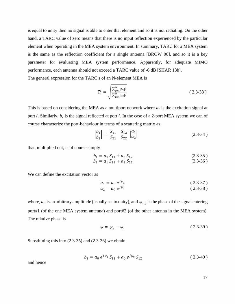
The general expression for the TARC s of an N-element MEA is
Γ𝑎𝑡 = √
∑ |𝑏𝑖|2𝑁
𝑖=1
∑ |𝑎𝑖|2𝑁
𝑖=1
( 2.3-33 )
This is based on considering the MEA as a multiport network where 𝑎𝑖 is the excitation signal at
port 𝑖. Similarly, 𝑏𝑖 is the signal reflected at port 𝑖. In the case of a 2-port MEA system we can of
course characterize the port-behaviour in terms of a scattering matrix as
[𝑏1𝑏2] = [
𝑆11 𝑆12𝑆21 𝑆22
] [𝑎1𝑎2] (2.3-34 )
that, multiplied out, is of course simply
𝑏1 = 𝑎1 𝑆11 + 𝑎2 𝑆12 (2.3-35 )
𝑏2 = 𝑎1 𝑆21 + 𝑎2 𝑆22 (2.3-36 )
We can define the excitation vector as
𝑎1 = 𝑎0 𝑒𝑗1 ( 2.3-37 )
𝑎2 = 𝑎0 𝑒𝑗2 ( 2.3-38 )
where, 𝑎0 is an arbitrary amplitude (usually set to unity), and 1,2
is the phase of the signal entering
port#1 (of the one MEA system antenna) and port#2 (of the other antenna in the MEA system).
The relative phase is
= 2−
1( 2.3-39 )
Substituting this into (2.3-35) and (2.3-36) we obtain
𝑏1 = 𝑎0 𝑒𝑗1 𝑆11 + 𝑎0 𝑒
𝑗2 𝑆12 ( 2.3-40 )
and hence
18
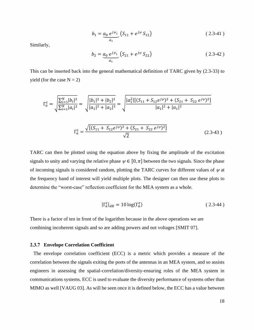
𝑏1 = 𝑎0 𝑒𝑗1 ⏟
𝑎1
(𝑆11 + 𝑒𝑗 𝑆12) ( 2.3-41 )
Similarly,
𝑏2 = 𝑎0 𝑒𝑗1 ⏟
𝑎1
(𝑆21 + 𝑒𝑗 𝑆22) ( 2.3-42 )
This can be inserted back into the general mathematical definition of TARC given by (2.3-33) to
yield (for the case N = 2)
Γ𝑎𝑡 = √
∑ |𝑏𝑖|2𝑁𝑖=1
∑ |𝑎𝑖|2𝑁𝑖=1
= √|𝑏1|2 + |𝑏2|2
|𝑎1|2 + |𝑎2|2= √
|𝑎12|[(𝑆11 + 𝑆12𝑒𝑗)2 + (𝑆21 + 𝑆22 𝑒𝑗)2]
|𝑎1|2 + |𝑎1|2
Γ𝑎𝑡 =
√[(𝑆11 + 𝑆12𝑒𝑗)2 + (𝑆21 + 𝑆22 𝑒𝑗)2]
√2 (2.3-43 )
TARC can then be plotted using the equation above by fixing the amplitude of the excitation
signals to unity and varying the relative phase ∈ [0, 𝜋] between the two signals. Since the phase
of incoming signals is considered random, plotting the TARC curves for different values of at
the frequency band of interest will yield multiple plots. The designer can then use these plots to
determine the “worst-case” reflection coefficient for the MEA system as a whole.
|Γ𝑎𝑡|𝑑𝐵 = 10 log(Γ𝑎
𝑡) ( 2.3-44 )
There is a factor of ten in front of the logarithm because in the above operations we are
combining incoherent signals and so are adding powers and not voltages [SMIT 07].
Envelope Correlation Coefficient
The envelope correlation coefficient (ECC) is a metric which provides a measure of the
correlation between the signals exiting the ports of the antennas in an MEA system, and so assists
engineers in assessing the spatial-correlation/diversity-ensuring roles of the MEA system in
communications systems. ECC is used to evaluate the diversity performance of systems other than
MIMO as well [VAUG 03]. As will be seen once it is defined below, the ECC has a value between

19
0 and 1; it approaches 1 in the presence of poor multipath propagation environment when the
different antenna elements start behaving like a single antenna [VAUG 87] [SHAR 13b]. On the
other hand, the MEA’s are said to ‘excite’ isolated wireless channels if the ECC value is equal to
zero [SHAR 17]. We can conclude that in order to obtain a high degree of diversity, and achieve
the improvements offered by MIMO (for example), one should aim to have zero or very low ECC
values for the individual antennas in an MEA system.
A. Basic Definition of ECC in Terms of Far-Zone Radiation Patterns
A truly rigorous derivation of the expression given below is very involved12, and so will not be
considered here. The envelope correlation coefficient between the i-th and j-th antennas in the
MEA system can be expressed, with integration over all solid angles (and an asterisk denoting
complex conjugation), as
𝜌𝑖𝑗 = ||∬𝑋𝑃𝐷×𝐸𝑖
𝜃(𝛺)𝐸𝑗𝜃∗(𝛺) 𝑃𝜃(𝛺)+𝐸𝑖
𝜙(𝛺)𝐸𝑗𝜙∗(𝛺) 𝑃𝜙(𝛺) 𝑑𝛺
√∬𝑋𝑃𝐷×𝐺𝑖𝜃(𝛺) 𝑃𝜃(𝛺)+𝐺
𝑖𝜙(𝛺) 𝑃𝜙(𝛺) 𝑑𝛺 √∬𝑋𝑃𝐷×𝐺𝑗
𝜃(𝛺) 𝑃𝜃(𝛺)+𝐺𝑗𝜙(𝛺) 𝑃𝜙(𝛺) 𝑑𝛺
||
2
(2.3-45)
where
𝐺𝑖𝜃(𝛺) = 𝐸𝑖
𝜃(𝛺)𝐸𝑖𝜃∗(𝛺) (2.3-46)
and denotes solid angle. XPD is the cross-polarization discrimination factor of the propagation
environment in which the MEA operates (and usually needs to be determined experimentally).
Functions 𝑃𝜃 and 𝑃𝜙 are the statistical distributions (one for each polarisation) describing the
probability of the incident field approaching from a specific direction. In a so-called isotropic
propagation environment XPD = 1 and 𝑃𝜃 = 𝑃𝜙 = 𝜋 4⁄ [VAUG 03]. In an isotropic
propagation environment expression (2.3-45) can be re-written as
12 R.Vaughan, Department of Engineering Science, Simon Fraser University, Canada. Private communication.

20
𝜌𝑖,𝑗 =|∬[ 𝐸𝑖 (𝛺) ∙ 𝐸𝑗∗ (𝛺) ] 𝑑𝛺 |
2
∬𝐸𝑖 (𝛺) ∙ 𝐸𝑖∗ (𝛺) 𝑑𝛺 ∬𝐸𝑗 (𝛺) ∙ 𝐸𝑗∗ (𝛺)𝑑𝛺
(2.3-47)
The electric field of the n-th antenna can be written
𝐸𝑛 (𝜃, 𝜙) = 𝐸𝑛𝜃(𝜃, 𝜙) 𝜃 + 𝐸𝑛
𝜙(𝜃, 𝜙)
(2.3-48)
Substituting this expression into the ECC definition (2.3-45), we obtain
𝜌𝑖,𝑗 =
|∫ ∫ 𝐸𝑖𝜃(𝜃,𝜙) 𝐸𝑗
𝜃∗(𝜃,𝜙) +𝐸𝑖𝜙(𝜃,𝜙) 𝐸𝑗
𝜙∗(𝜃,𝜙) 𝑠𝑖𝑛 𝜃 𝑑𝜃𝑑𝜙𝜋
𝜃=0
2𝜋
𝜙=0
|
2
∫ ∫ 𝐸𝑖𝜃(𝜃,𝜙) 𝐸𝑖
𝜃∗(𝜃,𝜙) +𝐸𝑖𝜙(𝜃,𝜙) 𝐸𝑖
𝜙∗(𝜃,𝜙) 𝑠𝑖𝑛 𝜃 𝑑𝜃𝑑𝜙𝜋
𝜃=0
2𝜋
𝜙=0
∫ ∫ 𝐸𝑗𝜃(𝜃,𝜙) 𝐸𝑗
𝜃∗(𝜃,𝜙) +𝐸𝑗𝜙(𝜃,𝜙) 𝐸𝑗
𝜙∗(𝜃,𝜙) 𝑠𝑖𝑛 𝜃 𝑑𝜃𝑑𝜙𝜋
𝜃=0
2𝜋
𝜙=0
(2.3-49)
The surface integrals in (2.3-49) can be converted into discrete summations for computation
purposes, a process that yields
𝜌𝑖,𝑗 =
|𝐹𝑖𝑗(𝜃, 𝜙)|2
𝐹𝑖𝑖(𝜃, 𝜙) 𝐹𝑗𝑗(𝜃, 𝜙)
(2.3-50)
where13,
𝐹𝑖𝑗(𝜃, 𝜙) = ∑ ∑[𝐸𝑖𝜃(𝜃𝑛, 𝜙𝑚) 𝐸𝑗
𝜃∗(𝜃𝑛, 𝜙𝑚) + 𝐸𝑖𝜙(𝜃𝑛, 𝜙𝑚) 𝐸𝑗
𝜙∗(𝜃𝑛, 𝜙𝑚)] ∆𝜃 ∆𝜙 𝑠𝑖𝑛 𝜃𝑛
𝑁
𝑛=0
𝑀
𝑚=0
(2.3-51)
𝐹𝑖𝑖(𝜃, 𝜙) = ∑ ∑ 𝐸𝑖𝜃(𝜃𝑛, 𝜙𝑚) 𝐸𝑖
𝜃∗(𝜃𝑛, 𝜙𝑚) + 𝐸𝑖𝜙(𝜃𝑛, 𝜙𝑚) 𝐸𝑖
𝜙∗(𝜃𝑛, 𝜙𝑚)𝑁𝑛=0 ∆𝜃 ∆𝜙 𝑠𝑖𝑛 𝜃𝑛
𝑀𝑚=0
(2.3-52)
𝐹𝑗𝑗(𝜃, 𝜙) = ∑ ∑ 𝐸𝑗𝜃(𝜃𝑛, 𝜙𝑚) 𝐸𝑗
𝜃∗(𝜃𝑛, 𝜙𝑚)+𝐸𝑗
𝜙(𝜃𝑛, 𝜙𝑚) 𝐸𝑗
𝜙∗(𝜃𝑛, 𝜙𝑚)
𝑁𝑛=0 ∆𝜃 ∆𝜙 𝑠𝑖𝑛 𝜃𝑛
𝑀𝑚=0
(2.3-53)
13 In Chapters 3 and 4, where these terms will be evaluated, the individual antenna patterns are sufficiently broad (and
the angular variations of the fields thus sufficiently ‘slow’) that use of = = 5 provides accurate evaluation of
the integrals.

21
The above expressions for computing ECC provide accurate results. However, a major drawback
to using this method is the requirement to measure or compute the 3D complex14 far-field patterns,
at every frequency point within the desired bandwidth of the MEA system. Therefore a simpler,
but approximate expression, has been derived in the literature for ECC calculation, as we will next
discuss.
B. Calculation in Terms of Multi-Port Scattering Parameters
Driven by the copious measurements and simulations which are involved in obtaining the
complex far-field 3D patterns, as well as the lengthy computation time required to calculate the
ECC via expression (2.3-50), researchers developed a simplified expression for the ECC [BLAN
03], namely
𝜌i,j =|𝑆𝑖𝑖∗ 𝑆𝑖𝑗 + 𝑆𝑗𝑖
∗ 𝑆𝑗𝑗|2
(1 − |𝑆𝑖𝑖|2 − |𝑆𝑗𝑖|2)(1 − |𝑆𝑗𝑗|
2− |𝑆𝑖𝑗|
2)
( 2.3-54 )
Expression (2.3-54) makes the assumption that antennas are lossless15, so that their radiation
efficiencies are unity (𝑒𝑖𝑟𝑎𝑑 = 𝑒𝑗
𝑟𝑎𝑑 = 1). Moreover, it should be highlighted that as the antenna
losses increase (efficiency decreases), the discrepancy between the correct values obtained from
(2.3-50) and those found using (2.3-54) becomes more significant [HALL 05]. One must be careful
when using the S-parameter approach as it often produces unrealistically low (optimistic) ECC
values which might lead the designer down the “garden path” [BHAT 17]. A good way of
understanding why finding the ECC using S-parameters is not accurate for lossy antennas is this16:
“Imagine going to the limit of extremely high loss. Then [S] just gives us the noise, which is
uncorrelated!". Finally, it should be noted that enhancing the isolation between the elements does
not guarantee a low ECC. This is because by definition the ECC is a measure of the signal
correlations and thus depends on the extent to which the radiated fields overlap [ASHR 21].
14 Amplitude and phase. 15 It s important to realise that this assumption is needed in order to arrive at (2.3-54) from the fundamental definition
of ECC. One should not assume that by using, in (2.3-54), the S-parameters for the actual lossy antennas that this
assumption is somehow removed. 16 R.Vaughan, Department of Engineering Science, Simon Fraser University, Canada. Private communication.

22
C. ECC Requirements for MIMO Antennas
Typically, an ECC value of less than 0.7 is sufficiently low for MEA at base stations. This
requirement drops to less than 0.5 for mobile terminals in order to achieve good diversity [VAUG
03]. Due to the presence of more elements in massive MIMO, signal correlation between non-
adjacent elements must be taken into account, and thus the ECC requirement in M-MIMO is
typically more stringent.
D. ECC Calculation Examples
In this section the expression (2.3-50) that we will call the far-field method, and expression
(2.3-54) that will be called the S-parameter method, will be used to compute the ECC for three
different examples. The resonances of three example antennas were chosen to be within the ISM
band (2.45 GHz - 5.8 GHz) to ensure that no discrepancies occur between the models studied due
to large frequency differences. The first deals with a lossless case, with two dipoles in free space
within proximity of each other. The second is like the first (that is, lossless) but with a loosely
coupled additional wire object present. The third case will be for two microstrip patch antennas
printed on a lossy substrate.
Figure 2.3-3 shows the two dipole antennas parallel to each other and separated along the x-axis,
in free space. The dipoles are identical, and each has a dedicated port. This two-dipole MEA was
modelled as consisting of thin wires using the full-wave electromagnetic simulation software based
on the method of moments [FEKO 18], and the antennas’ scattering parameters and far-field
patterns computed.
Figure 2.3-3: Two closely spaced dipole antennas

23
The simulation data from FEKO was then run through a script17 to calculate the ECC. Figure 2.3-4
shows the computed ECC for the two-dipole example using the far-field method and the S-
parameter method. The two sets of results are identical, as might be expected because the dipoles
are lossless (perfect conductors).
Figure 2.3-4: ECC plots for dipole antennas
Since Figure 2.3-4 shows identical results using either method, we decided to try the slightly
altered arrangement shown in Figure 2.3-5, in which a loosely-coupled additional wire has been
introduced at the origin and lies along the y-axis. The passive wire introduces some slight
discrepancy between the two ECC curves, as seen in Figure 2.3-6, but are still practically identical.
We can conclude that the S-parameter approach for computing the ECC is a very good
approximation for lossless antennas. The comparison also serves to validate the script that
implements expression (2.3-50) to find the ECC based on the definition of this quantity.
17 Developed by the author in MATLAB.

24
Figure 2.3-5: Two dipole antenna and a passive wire.
Figure 2.3-6: ECC results for two dipole antennas and a passive wire
We now compare the outcomes of the two expressions for the ECC when the antennas in the MEA
are lossy. Figure 2.3-7 shows a simple symmetrical design of two pin-fed patch antennas etched
on a substrate with r 4 = and tan 0.005 = is simulated. Figure 2.3-8 reveals a slight discrepancy
between the computed ECC values which is roughly about 1%. Moreover, Figure 2.3-9 shows how
the S-parameter approach can lead to inaccurately low ECC values.

25
Figure 2.3-7: Two patch antennas on a lossy substrate with 𝜺𝒓 = 𝟎. 𝟎𝟒 and 𝒕𝒂𝒏(𝜹) = 𝟎. 𝟎𝟎𝟓.
Figure 2.3-8: ECC curves for the two patch antennas shown in Figure 2.3-7.

26
To develop a sense of how the lossy-ness affects the ECC calculation, we recalculated the ECC
for the same two-patch MEA design, but with the loss tangent of the substrate increased to
tan 0.01 = and then tan 0.025 = , the results being provided in Figure 2.3-9 and Figure 2.3-10,
respectively. These show that as the amount of loss increases the ECC computed using (2.3-50) -
the correct result - stays largely the same but that the result found using the S-parameters moves
further from the correct result to increasingly lower (over optimistic) values. This serves to
highlight the importance of using complex 3D far-field patterns in the calculation of the ECC.
Figure 2.3-9: ECC curves for the two patch antennas shown in Figure 2.3-7 but with tan𝛿 = 0.01.

27
Figure 2.3-10: ECC curves for the two patch antennas shown in Figure 2.3-7 but with tan𝛿 = 0.025
The Need for Low Mutual Coupling Between MIMO Antennas
It is widely accepted18 among MIMO antenna designers that low mutual coupling is required in
order to achieve good diversity. Numerous studies have shown that mutual coupling can have a
negative effect on the correlation between channels, and thus ultimately a deleterious effect on the
capacity of the MIMO system. In cases where the inter-element separation distance is less
than 0.5 𝜆, strong mutual coupling exists and it can cause a decrease in the channel capacity,
especially so as the number of antenna elements increases [JANA 02], [ABOU 06]. The conclusion
is that mutual coupling effects are detrimental to MIMO performance. We would like it to be as
low as possible.
As stated in [OZDE 03], arguments both for and against mutual coupling in MIMO are correct for
different scenarios. In environments with poor scattering (highly correlated environment), if the
mutual coupling effect is allowed to deform19 the far-field radiation pattern, this might serve as a
decorrelation factor. However, if the environment is rich in multipath scattering, and the separation
18 The are some works which suggest that mutual coupling can in fact serve as a decorrelation factor (and thus be
advantageous), thereby increasing the channel capacity [SVAN 01] [CLER 03] [BORJ 03], but this does not at present
to be the majority opinion of wireless communication theory experts. 19 Which might be undesirable for other reasons.

28
distance between adjacent elements is less than 0.5𝜆, mutual coupling between the antenna
elements is non-negligible and it increases the correlation.
It should be noted that even for signals propagating in a poor environment, the decorrelation effect
due to mutual coupling is only significant for very small separation distances(0.1𝜆 − 0.2𝜆)
between the MIMO antennas.
MIMO was developed to overcome the deep fades resulting from multipath propagations in rich
scattering environments. Knowing this, we will in this thesis always assume that mutual coupling
impedes MIMO performance and we will work to reduce it.
Technical Definition of Mutual Coupling
We can quantify mutual coupling between any number of antennas via network theory. If we
assume an MEA with N-elements, then we can develop and equivalent N-port network; that is a
network with N-inputs or N-outputs [VAUG 03]. For simplicity we will consider two antennas,
which form a two-port network, and can then formulate the impedance matrix [𝑍] so that
[ ] [ ][ ]V Z I= , in other words
[𝑉1𝑉2] = [
𝑍11 𝑍12𝑍21 𝑍22
] [𝐼1𝐼2] ( 2.3-55 )
where 𝑍𝑚𝑛 = 𝑅𝑚𝑛 + 𝑗𝑋𝑚𝑛 and is known as the self-impedance for (𝑚 = 𝑛), and the mutual
impedance (𝑚 ≠ 𝑛) between ports 𝑚 and 𝑛. If we write out the compact notation (2.3-55) in full,
we of course have [STUT 13]
𝑉1 = 𝑍11 𝐼1 + 𝑍12 𝐼2 ( 2.3-56 )
𝑉2 = 𝑍21 𝐼1 + 𝑍22 𝐼2 ( 2.3-57 )
where the mutual impedances are
𝑍12 =𝑉1
𝐼2|𝐼1=0
, 𝑍21 =𝑉2
𝐼1|𝐼2=0
( 2.3-58 )
and the self-impedances of the antennas are
𝑍11 =𝑉1
𝐼1|𝐼2=0
, 𝑍22 =𝑉2
𝐼2|𝐼1=0
(2.3-59 )
The input impedances seen by each of the antenna elements are (under operational conditions)
𝑍𝑖𝑛1 =
𝑉1𝐼1= 𝑍11 + 𝑍12 (
𝐼2𝐼1)
( 2.3-60 )

29
𝑍𝑖𝑛2 =
𝑉2𝐼2= 𝑍21 (
𝐼1𝐼2) + 𝑍22
( 2.3-61 )
This implies that the impedance seen at one antenna is affected by the impedance of the “other”
antenna due to mutual coupling. The amount of mutual coupling in a system is captured in the off-
diagonal terms in the scattering matrix, or 𝑆12 in this two-antenna case. We are able to transform
impedance matrix terms [𝑍] into scattering matrix parameters [𝑆] by using the following equations
[POZA 98].
𝑆11 = (𝑍11 − 𝑍0)(𝑍22 + 𝑍0) − 𝑍12𝑍21(𝑍11 + 𝑍0)(𝑍22 + 𝑍0) − 𝑍12𝑍21
( 2.3-62 )
𝑆12 =2𝑍12𝑍0
(𝑍11 + 𝑍0)(𝑍22 + 𝑍0) − 𝑍12𝑍21
( 2.3-63 )
𝑆21 =2𝑍21𝑍0
(𝑍11 + 𝑍0)(𝑍22 + 𝑍0) − 𝑍12𝑍21
( 2.3-64 )
𝑆22 = (𝑍11 + 𝑍0)(𝑍22 − 𝑍0) − 𝑍12𝑍21(𝑍11 + 𝑍0)(𝑍22 + 𝑍0) − 𝑍12𝑍21
( 2.3-65 )
This enables us to connect the S-parameter representations (used previously in Sections 2.3.6 and
2.3.7) to the mutual impedance viewpoint. In this thesis ‘mutual coupling’ will mean ijS .
Inter-Element Coupling Requirements in MIMO Systems
Having established that mutual coupling can degrade the performance of MIMO systems, an
important question arises: How low does the mutual coupling need to be? An attempt to answer
this question was made in [MEI 18], by conducting a measurement campaign for antennas with
different mutual coupling values. The antennas studied were inverted-F antennas (IFA’s) which
made use of a lumped capacitor for decoupling. The capacitance of the lumped element was varied
to yield different decoupling (mutual coupling) values, while all other antenna parameters
remained the same. The testing was performed in a chamber which made use of the Umi (micro-

30
cell) and Uma (macro-cell) channel models which are the standard channel models for urban LTE
MIMO micro- and macro- cell testing, respectively.
Figure 2.3-11: Data throughput versus received power for antennas with different levels of mutual coupling.
Macro-cell on the left and micro-cell on the right. (After [MEI 18])
The results are shown in Figure 2.3-11. They display the maximum data throughput achieved by
the antennas for different received power levels. The mutual coupling levels of the labelled
antennas are : A (-11 dB), B (-13 dB), C (-16 dB), D (-20 dB) and E (-30 dB). The return loss is
between -14 and -15 dB for all antenna types, and the effeciency between 80% and 84%. The
measured results, for both scenarios, show that the throughput seems to increase as the mutual
coupling is decreased. From the observation that there is no significant throughput increase in
going from type E (-30 dB) to type D (-20 dB) it was concluded that -20 dB of mutual coupling
is sufficient for good MIMO performance [MEI 18].
Other works have reported that mutual coupling of -15 dB is enough for ultra-wide-band MIMO
[LEI 13]. For massive-MIMO basestations, the industry rule of thumb rule is more restrictive, as
it requires mutual coupling to be -30 dB or lower [CHEN 18]. In Chapters 3 and 4 of this thesis
we will work to decouple antennas by setting an upper limit to the mutual coupling and not defining
a lower limit. This will allow the shaping process to minimize mutual coupling as much as possible
within the rules of physics.

31
Radiation Pattern Requirement for MIMO Antennas
Different propagation environments require different antennas, yet we should design an antenna
which would yield acceptable performance in a range of environments. For an antenna to be
effective in a MIMO system it must enhance the channel capacity by illuminating as much of the
propagation environment as possible to encourage multipath propagation. Antennas which allow
signals to be transimitted and received over a wide range of angles increase the channel capacity
in MIMO systems [BALA 16]. For this reason, an isotropic antenna would be ideal for MIMO
applications, but of course such antennas are not physically possible. The conclusion of a number
of MIMO measurement campaigns [WITT 09] [LI 14] was that antennas with broad beams are
best.
Existing Coupling Reduction Methods in MEA Systems
Preliminary Notes
This section will deal with the existing methods for antenna decoupling in the literature. We
will attempt to briefly explain the principles of each method and discuss selected examples, and
list reported advantages and disadvantages offered by each approach. We will classify the methods
that have so far been used for coupling reduction as eigenmode decomposition schemes, inserted
component schemes, coupled resonator schemes, and decoupling surface schemes. We also
indicate where some sort of automated optimization has been used in in the design of MEA systems
for MIMO applications. There are some existing methods which attempt to mitigate the effects of
mutual coupling using various digital signal processing schemes. However as [CHEN 18] stated it
is never a good idea to hope that the unwanted coupling can be completely removed using such an
approach. It is better to design the MEA elements so that they have low coupling, and then (if
necessary) use signal processing to make relatively small improvements.
Eigenmode Decomposition Schemes
This method is based on the excitation of N orthogonal modes denoted as (𝐽𝑛) for an N-element
MIMO system. The modes correspond to surface currents which exist on the conductor geometry
under study. Each mode has an associated radiation pattern. The orthogonal electromagnetic
modes are obtained for the eigenvalues of the method of moment impedance matrix. Essentially,

32
the (orthogonal) modes are (orthogonal) solutions to Maxwell’s equations. Since each
characteristic mode yields a radiation pattern, in a multipath environment one radiation pattern of
the antenna might undergo fading while the other radiation pattern does not. As a result, if the right
modes are excited good antenna diversity can be achieved [SVAN 02]. This method has been
shown to provide significant improvement in cases where the antennas are highly correlated over
a narrow bandwidth. Characteristic modes research in MIMO has given rise to a multimode
antenna which is essentially a single antenna structure fed through one or more ports. Each feed
excites a set of orthogonal modes which allow the antenna to behave as a multi antenna system.
One of the obvious advantages of such designs is their compactness which waive the need for
multiple physical antenna or decoupling surface structures. The authors of [SVAN 02] propose the
use of multi-mode antennas to increase MIMO channel capacity without the use of additional
antenna elements. The additional modes which are excited essentially represent different solutions
to Maxwell’s equations that fulfill the boundary conditions for the geometry at hand. The author
shows how a single circular microstrip antenna can be excited with two modes to achieve higher
diversity.
In [MANT 16], the theory of characteristic modes is utilized to design massive MIMO MEA’s.
The design is comprised of an 11 by 11 planar array arrangement of physical antennas which are
excited by four ports each. Figure 2.4-1 shows the four ports carefully placed in order to excite
four orthogonal characteristic modes effectively yielding 121 × 4 = 484 antennas with good
isolation and reflection coefficients.
Figure 2.4-1: Four ports feeding a single multimode antenna [MANT 16]

33
Among the many interesting works which were conducted on MEA design using theory of
characteristic modes (TCM), is that of [LI 12], where the characteristic modes excited on the
mobile station’s chassis (ground) were studied in order to determine the different antenna
placements. In this study, it was revealed that if one considers the magnitude of the electric field
resulting from the first characteristic mode shown in Figure 2.4-2, the designer could obtain better
isolation by placing the antennas closer to each other. This is of course done by studying the results
in Figure 2.4-2 which shows the normalized magnitude of the E-field of the dominant characteristic
mode (at 𝑓 = 1.35 GHz) over the entire area (100 mm x 40 mm) of the mobile device’s chassis
which is shown at the bottom of the figure. The characteristic mode (CM) has a sinusoidal
behaviour. Therefore, placing one antenna at the location of the electric field’s maxima (edge of
vertical component of chassis) and the other at the electric field’s minima (center of chassis) will
yield better isolation. The insight offered by TCM analysis produced an unintuitive result in which
the center-edge placement (less distance) yields better isolation compared to the edge-edge
placements (more distance).
Figure 2.4-2: Normalized magnitude of the total electric field of first CM vs. chassis geometry [LI 12]
Inserted Component Schemes
The most popular inserted component schemes entail inserting a parasitic element which acts as
a decoupling structure. Such structures are usually made of perfect electric conductor (PEC) and
work to deflect surface and space waves radiated by an antenna away from the other antennas in
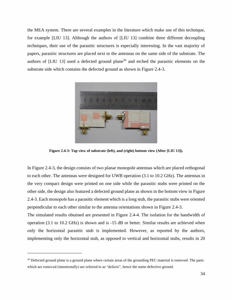
34
the MEA system. There are several examples in the literature which make use of this technique,
for example [LIU 13]. Although the authors of [LIU 13] combine three different decoupling
techniques, their use of the parasitic structures is especially interesting. In the vast majority of
papers, parasitic structures are placed next to the antennas on the same side of the substrate. The
authors of [LIU 13] used a defected ground plane20 and etched the parasitic elements on the
substrate side which contains the defected ground as shown in Figure 2.4-3.
Figure 2.4-3: Top view of substrate (left), and (right) bottom view (After [LIU 13]).
In Figure 2.4-3, the design consists of two planar monopole antennas which are placed orthogonal
to each other. The antennas were designed for UWB operation (3.1 to 10.2 GHz). The antennas in
the very compact design were printed on one side while the parasitic stubs were printed on the
other side, the design also featured a defected ground plane as shown in the bottom view in Figure
2.4-3. Each monopole has a parasitic element which is a long stub, the parasitic stubs were oriented
perpendicular to each other similar to the antenna orientations shown in Figure 2.4-3.
The simulated results obtained are presented in Figure 2.4-4. The isolation for the bandwidth of
operation (3.1 to 10.2 GHz) is shown and is -15 dB or better. Similar results are achieved when
only the horizontal parasitic stub is implemented. However, as reported by the authors,
implementing only the horizontal stub, as opposed to vertical and horizontal stubs, results in 20
20 Defected ground plane is a ground plane where certain areas of the grounding PEC material is removed. The parts
which are removed (intentionally) are referred to as “defects”, hence the name defective ground.

35
dB increase for S11 in the 8 - 10 GHz bandwidth. As such two stubs are implemented to isolate the
antennas and minimize the return loss.
Figure 2.4-4: S21 Plots: (- . - ) no parasitic stubs, (- - -) only vertical stub, (....) horizontal stub only, and (____)
both stubs (After[ LIU 14]).
A thorough study presented in [YANG 03] focused on decoupling MEA antennas using
electromagnetic bandgap (EBG) structures. An EBG structure is a periodic structure consisting of
small parasitically-excited elements usually placed in between the antenna elements and is used to
decouple the antenna elements by supressing the surface waves present on the substrate.
Effectively, the EBG can be thought of as a band-stop filter for surface waves. Two rectangular
microstrip antennas operating at 5.8 GHz [YANG 03], with their E-planes coincident (“E-plane
coupling” case is the term used) were considered as depicted in Figure 2.4-5, with the spacing
between the patches being about 38.8 mm (or 0.75 𝜆5.8 𝐺𝐻𝑧).
Figure 2.4-5: EBG and two patch antennas coupled in E-Plane. (After [YANG 03])

36
The EBG structure presented in [YANG 03] consists of 3 mm square mushroom-like patches and
has an inter-element spacing of 0.5 mm. This mushroom-like EBG consists of 4 main components:
a ground plane, a dielectric substrate, square patches, and vias which connect the patches to the
ground plane. As seen in Figure 2.4-6, the introduction of the EBG resulted in 8 dB reduction in
the coupling levels and enhanced the return loss of the antennas by about 3 dB. However, one
general drawback of EBG’s is the valuable space which is wasted in inter-element separation.
Additionally, this particular mushroom-like EBG is inherently difficult to implement as it requires
intricate manufacturing to connect the EBG elements’ vias to ground.
Figure 2.4-6: Measured results of microstrip antennas with and without EBG.
Coupled Resonator Schemes
This method includes the neutralization line (NL) and the defected ground (DG) methods. The
neutralization line (NL) is a microstrip link that connects two antennas and acts as a neutralization
device by picking up some of the mutual coupling signal on antenna B and returning it out of phase
to Antenna A, hence reducing or “neutralizing” the mutual coupling effect [DIAL 06]. Good
results are achieved when the NL technique is implemented. However, it has been shown that this
method is only effective for narrow band applications. Since the dimensions of microstrip lines
are dependent on frequency, decoupling antennas at low frequencies such as the GSM band (800-

37
900 MHz) would require a NL with large physical area and is not feasible. Other coupled resonator
methods include the defected ground plane method which entails removing parts of the PEC that
makes up the ground plane of a substrate. The dimensions of the removed parts are selected
carefully in order to reduce mutual coupling between the antenna elements. However, this method
can lead to a decrease in the gain of the MEA. Specifically, in printed MEA’s having a defected
ground will always lead to a deteriorated Front-to-Back ratio in the far-field patterns. This is a
result of radiation which “leaks” through the defected ground plane.
The first design intended to decouple antennas using the NL technique is [DIAL 06]. Although the
term is not explicitly mentioned in this paper, the author makes use of a microstrip line suspended
between two PIFA’s to neutralize the coupling by producing an opposite coupling signal in order
to enhance isolation. The PIFA’s consisted of different sizes which were intended to operate at
different frequencies. Both PIFAs were placed on top of a finite ground structure as shown in
Figure 2.4-7.
Figure 2.4-7: PIFA antennas on PCB (After [DIAL 06])
Before arriving at the arrangement shown above, [DIAL 06] conducted a study to better understand
how different positioning would affect the S-parameter response of the entire system. It was later
found that placing the PIFAs in the above arrangement provides maximum isolation for the entire
desired band of operation. Figure 2.4-9 shows the S-parameter response of the antenna
arrangement shown above, where the shorting strips of the antennas are facing each other and the
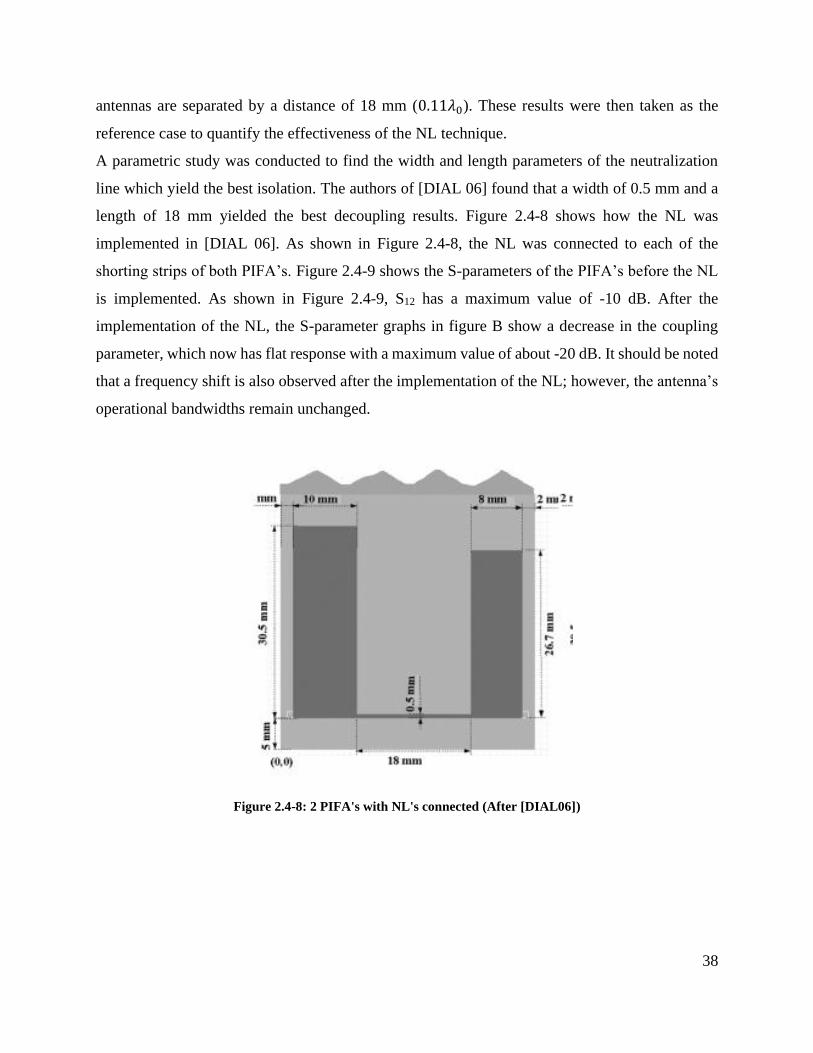
38
antennas are separated by a distance of 18 mm (0.11𝜆0). These results were then taken as the
reference case to quantify the effectiveness of the NL technique.
A parametric study was conducted to find the width and length parameters of the neutralization
line which yield the best isolation. The authors of [DIAL 06] found that a width of 0.5 mm and a
length of 18 mm yielded the best decoupling results. Figure 2.4-8 shows how the NL was
implemented in [DIAL 06]. As shown in Figure 2.4-8, the NL was connected to each of the
shorting strips of both PIFA’s. Figure 2.4-9 shows the S-parameters of the PIFA’s before the NL
is implemented. As shown in Figure 2.4-9, S12 has a maximum value of -10 dB. After the
implementation of the NL, the S-parameter graphs in figure B show a decrease in the coupling
parameter, which now has flat response with a maximum value of about -20 dB. It should be noted
that a frequency shift is also observed after the implementation of the NL; however, the antenna’s
operational bandwidths remain unchanged.
Figure 2.4-8: 2 PIFA's with NL's connected (After [DIAL06])

39
Figure 2.4-9: The S-parameter response before introducing the NL (After [DIAL 06])
Figure 2.4-10: The S-parameter response after introducing the NL (After [DIAL 06])

40
During the parametric study which was conducted by [DIAL 06] for the NL, it was noted that
increasing the width and/or the length of the NL, results in shift of the null in S12 graph. As such,
if the antenna designer intends to decouple antennas at lower frequencies, a longer and/or thicker
NL is needed. This relationship between the size of the NL and frequency is a limitation of this
method. Although the NL provides good results for decoupling at high frequencies, implementing
a NL on a mobile unit operating at lower frequencies (eg 900 MHz) is not feasible.
NL have been also reported to have narrow decoupling bandwidth for antennas other than PIFA’s.
There have been recent studies which were successful at introducing variations to the NL in an
effort to increase the decoupling bandwidth. Among those studies is [ZHAN 16] where the two
monopoles shown in Figure 2.4-11, were designed for an (3.1 – 5 GHz) Ultra Wide Band (UWB)
MIMO application. As seen in Figure 2.4-11, a circular disk was inserted in the NL in order to
widen the decoupling bandwidth of the NL. Moreover, the NL was placed on top of the ground
plane to allow for a more compact design.
s
Figure 2.4-11: Design of two Antennas with NL (After [ZHAN 16])
Impressive decoupling results were achieved as shown in Figure 2.4-12 below, the maximum S21
value was reduced from -8 dB to – 20 dB. However, the S11 graph value was degraded by a few
dB. Nonetheless, the authors successfully decoupled the UWB monopole antennas using NL.

41
Figure 2.4-12: S-parameters with and without NL (After [ZHAN 16])
Decoupling Surface Schemes
The decoupling surface is similar to an EBG, however, one key difference is that the decoupling
surface (DS) is not usually made up of regular shapes, such as rectangles or squares, and is not
periodic. Additionally, EBG’s are usually placed in the same plane of the antennas (coplanar)
whereas DS can be implemented in a non-coplanar fashion. In such schemes a decoupling surface
might or might not be coplanar with the radiating elements.
Before we begin the discussion of Decoupling Surfaces (DS), we must first take note of the
differences between EBG’s and DS. Designs which entail the use of EBG’s have the EBG typically
placed in between the antenna elements, whereas a DS can be placed anywhere near the antennas.
As such, the DS offers more flexibility in design. Among the studies completed on DS schemes is
that of [WEI 17] where a simple decoupling surface was used to decouple four printed quasi-yagi
antennas, operating at 5.5 GHz. The antennas are co-linear as shown in Figure 2.4-13. The DS
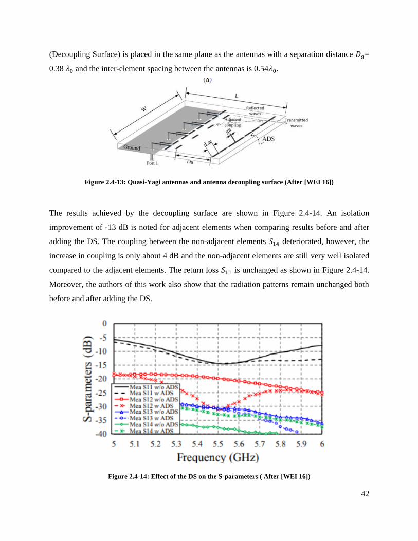
42
(Decoupling Surface) is placed in the same plane as the antennas with a separation distance 𝐷𝑎=
0.38 𝜆0 and the inter-element spacing between the antennas is 0.54𝜆0.
Figure 2.4-13: Quasi-Yagi antennas and antenna decoupling surface (After [WEI 16])
The results achieved by the decoupling surface are shown in Figure 2.4-14. An isolation
improvement of -13 dB is noted for adjacent elements when comparing results before and after
adding the DS. The coupling between the non-adjacent elements 𝑆14 deteriorated, however, the
increase in coupling is only about 4 dB and the non-adjacent elements are still very well isolated
compared to the adjacent elements. The return loss 𝑆11 is unchanged as shown in Figure 2.4-14.
Moreover, the authors of this work also show that the radiation patterns remain unchanged both
before and after adding the DS.
Figure 2.4-14: Effect of the DS on the S-parameters ( After [WEI 16])

43
A more sophisticated DS was designed in [WU 17]; a cross section of the design is shown in Figure
2.4-15. The setup comprised of 2-by-2 dual polarized dipole antennas. Each of the dual polarized
antennas was made of two perpendicularly oriented dipole antennas, which the authors refer to as
cross-dipole antennas. The individual antennas in the cross-dipole elements were oriented at
45𝑜and at 135𝑜 with respect to the horizontal axis. This arrangement yielded a total of eight
antenna elements. The antennas were designed to operate at 3 GHz – 3.8 GHz and were placed on
top of a ground plane while the decoupling surface was etched on a separate substrate which was
placed on top (non-coplanar) of the antenna elements.
Figure 2.4-15: (a) Antennas and DS (b) Cross dipole arrangement (after [WU 17])
The substrate was selected to be a low-loss one with tan(𝛿) = 0.001 and a thickness of 1 mm in
order to maintain the radiation efficiency of the antennas. Horizontally adjacent antennas were
separated by 45 mm (0.51 𝜆0) and vertically adjacent antennas were separated by 60
mm (0.68 𝜆0). The results reported in [WU 17] are shown in Figure 2.4-16 where it can be seen
that that the decoupling surface greatly reduces the mutual coupling between co-polarized and
horizontally adjacent elements as in the case of 𝑆13 which is reduced from -14 dB to -25 dB. In the
case of cross-polarized horizontally adjacent elements, such as 𝑆14 and 𝑆23, the coupling is slightly
improved by 2 dB and about 6 dB, respectively.
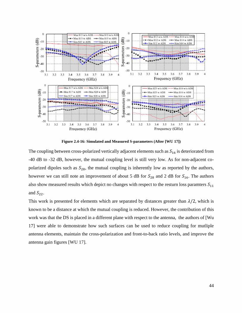
44
Figure 2.4-16: Simulated and Measured S-parameters (After [WU 17])
The coupling between cross-polarized vertically adjacent elements such as 𝑆16 is deteriorated from
-40 dB to -32 dB, however, the mutual coupling level is still very low. As for non-adjacent co-
polarized dipoles such as 𝑆28, the mutual coupling is inherently low as reported by the authors,
however we can still note an improvement of about 5 dB for 𝑆28 and 2 dB for 𝑆16. The authors
also show measured results which depict no changes with respect to the resturn loss paramters 𝑆11
and 𝑆22.
This work is presented for elements which are separated by distances greater than 𝜆/2, which is
known to be a distance at which the mutual coupling is reduced. However, the contribution of this
work was that the DS is placed in a different plane with respect to the antenna, the authors of [Wu
17] were able to demonstrate how such surfaces can be used to reduce coupling for mutliple
antenna elements, maintain the cross-polarization and front-to-back ratio levels, and improve the
antenna gain figures [WU 17].

45
Existing Use of Optimization in MIMO Antenna Design
There is limited literature for MIMO MEA system designs involving optimization, and none that
use actual shape synthesis21. In [KARL 09], three cases are presented as examples for utilizing
particle swarm optimization in MEA design. In this study, a feeding network for the MEA’s is
optimized, the antenna’s impedances as well as the feeding network are modeled in an equivalent
circuit with lumped elements, the value of each of the lumped elements (capacitance, inductance
or resistance) is then optimized in order to arrive at a desired design objective. In the first example
included in [KARL 09], an RLC circuit is used as an equivalent model to a feed network for two
dipole antennas of equal length, the circuit’s lumped element values are then optimized to achieve
a higher radiation efficiency. The optimization does result in ~ 8% increase in the radiation
efficiency. The second example studies two inverted-F antennas (IFA’s) which are placed in an
orthogonal arrangement with respect to each other. The IFA’s were designed to operate at 1.8 GHz,
the portion of IFA’s which extends parallel to the ground was then shortened (physically cut), and
the optimization process was run for the feeding network of the antennas. Optimization was
conducted for two objectives: first, to arrive at the highest possible diversity gain between both
antennas and second, to recover the radiation efficiency lost after the antennas were shortened.
Diversity gain is a measure of the effect of diversity on the communication system with respect to
SNR, uncorrelated signals received on different channel paths will increase the SNR level at the
receiver when these signals are combined [SHAR 13]. The measurement results of the second
optimized design are shown in Figure 2.4-17 and Figure 2.4-18.
21 This is done in the present thesis for the first time.

46
Figure 2.4-17: Efficiency of the antennas before and after optimization (After [KARL 09])
Figure 2.4-18: Diversity Gain before and after optimization (After [KARL 09])
In [BEKA 16], parameter optimization is performed for two monopole antennas in order to obtain
a reduced size antenna with good electrical performance. The design process starts with a pre-
defined geometry of the UWB printed monopole antenna in Figure 2.4-19. The dimensions of the
geometrical features shown in Figure 2.4-19 are then optimised to reduce the value of some
objective function defined in terms of the desired performance parameters, as needs to be done
whenever optimization is used.

47
Figure 2.4-19: Monopole parameters to be optimized, (b) 3D view of the monopole antenna
(After [BEKA 16])
The fitness function reported by the authors contains an objective function which selects the
antenna with the smallest footprint (𝑎1 × 𝑎2) as the most-fit antenna, as well as a constraint
function which calculates the value of (max|𝑆11| + 𝑆𝑚𝑎𝑥)/𝑆𝑚𝑎𝑥 , where 𝑆𝑚𝑎𝑥 = −12.5 𝑑𝐵.
Both the objective function and the penalty function are summed to yield the final value of the
fitness function. Keeping in mind that the goal of the optimizer is to arrive at a design which
minimizes the fitness function, if the value of S11 exceeds the threshold of -12.45 dB, the fitness
function value increases and the design is considered “less fit”. Similarly, if the design yields a
large footprint, it is considered “less fit”. Figure 2.4-20 shows the simulated S11 results of the initial
and the optimized antenna.
Figure 2.4-20: S11 simulation results for initial (- -) and optimized (___) antennas (After [BEKA 16])
After the optimization process is completed the “most-fit” antenna is replicated and combined by
the designer to arrive at the final MIMO antenna design. Figure 2.4-21 shows the optimum design
from [BEKA 16], while Figure 2.4-22 shows simulated results of the combined antennas in the
final design. It should be noted that this study takes advantage of two other isolation methods in
addition to optimization. First, there is a neutralization line connecting the two different antennas
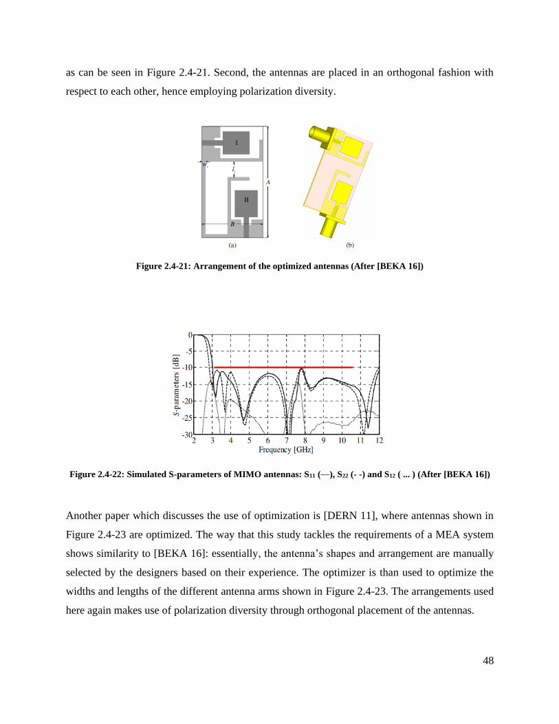
48
as can be seen in Figure 2.4-21. Second, the antennas are placed in an orthogonal fashion with
respect to each other, hence employing polarization diversity.
Figure 2.4-21: Arrangement of the optimized antennas (After [BEKA 16])
Figure 2.4-22: Simulated S-parameters of MIMO antennas: S11 (___), S22 (- -) and S12 ( ... ) (After [BEKA 16])
Another paper which discusses the use of optimization is [DERN 11], where antennas shown in
Figure 2.4-23 are optimized. The way that this study tackles the requirements of a MEA system
shows similarity to [BEKA 16]: essentially, the antenna’s shapes and arrangement are manually
selected by the designers based on their experience. The optimizer is than used to optimize the
widths and lengths of the different antenna arms shown in Figure 2.4-23. The arrangements used
here again makes use of polarization diversity through orthogonal placement of the antennas.

49
Figure 2.4-23: Initial antenna arrangement "pre-optimization" (After [DERN 11])
The objectives are selected to maximize the radiation efficiency, minimize the envelope correlation
coefficient (ECC), and to minimize the total enclosed antenna area. The authors describe the
scattering efficiency of an element “a” as 𝜂𝑥.
𝜂1 = 1 − |𝑆11|2 − |𝑆21|
2 ( 2.4-1 )
𝜂2 = 1 − |𝑆12|2 − |𝑆22|
2 ( 2.4-2 )
The “scattering efficiencies” for both elements can then be averaged,
𝜂𝑎𝑣𝑔 =
𝜂1 + 𝜂22
( 2.4-3 )
The ECC can be calculated below as shown below,
𝜌𝑒 =
|𝑆11 𝑆12∗ + 𝑆12𝑆22
∗ |
𝜂1𝜂2
( 2.4-4 )
The authors of [DERN 11] then use what they refer to as MIMO efficiency which is calculated
from the correlation coefficient
𝜂𝑀𝐼𝑀𝑂 = √𝜂1𝜂2(1 − 𝜌𝑒) ( 2.4-5 )

50
Each of the above objectives (antenna area, 𝜂𝑀𝐼𝑀𝑂 and average radiation efficicncy) was treated
as a separate fitness function therefore the designer had to select the weights for each of the
objectives. It should be noted that this is a multi-objective optimization which is different from the
single objective optimization where the values are summed, as was done in [BEKA 16]. Using a
multi-objective approach allows the designer to select the weights of the objectives after the
simulation begins. In contrast, in a single objective design environment the weights of each term
must be determined by the designer before the optimization process starts.
Figure 2.4-24: Different results of the simulation.
Figure 2.4-24 shows a selected sample of the results achieved by different design trials of the
optimizer. The vertical axis represents the total area (footprint) of the antenna in millimeters, the
horizontal axis represents the average radiation efficiency in decibels (𝜂𝑎𝑣𝑔), and the color
gradient represents the “MIMO efficiency” (𝜂𝑀𝐼𝑀𝑂) which is used by the author to calculate the
correlation coefficient. The optimum design selected is highlighted with a circle in Figure 2.4-24,
this selection is based on a trade-off between all three objectives considered in this study (average
radiation efficiency, antenna area, and MIMO efficiency). The weights of the optimum design
were found to be 0.38, 0.36 and 0.26 for (𝜂𝑎𝑣𝑔), (𝜂𝑀𝐼𝑀𝑂) and antenna area, respectively. The

51
simulated results of the optimized design are shown in Figure 2.4-25 and Figure 2.4-26.
Unfortunately, the design does not report any initial (pre-optimization) results for comparison.
Figure 2.4-25: Simulated S-parameter of the optimized design (After [DERN 11]).
Figure 2.4-26: Simulated radiation efficiencies, average efficiency, and MIMO efficiency (After [DERN 11]).

52
Computational Approach Harnessed in the Thesis for Shape Synthesis
The research in this thesis makes heavy use of computational electromagnetics (CEM) to achieve
its goals. It does not, however, undertake research or development on CEM methods themselves.
Instead, it uses the commercially available computational engine known as the Hyperworks/FEKO
suite [FEKO 18]. The background material is truly well-known, and adequately described in the
textbook literature, amongst which are [PETE 97], [VOLA 12] and [KRIS 16]. The structure under
study is composed of perfectly conducting shapes located on dielectric substrates of finite
thickness, some of which may be backed by perfectly conducting “ground planes”. The
electromagnetics problem to be modelled is driven by concentrated sources that allow one to define
antenna feedpoint locations (ports). The electric current density on the conducting surfaces forms
the unknown quantity in an integral equation that constitutes the rigorous full-wave
electromagnetic model of the geometry. This model is solved numerically using the moment
method (MM), the presence of the substrate material being accounted for through the use of a
special Green’s function [JAKO 00] in the integral equation. Once the current density has been
found in this way, the electromagnetic fields everywhere (eg. far-zone patterns; near-zone fields)
may be found, and all the antenna figures of merit22 defined in Section 2.3.
A software code associated with FEKO, called Hyperstudy [HYPE 20], allows the user to divide
the conducting surfaces into rectangular cells, define objective functions in terms of the
performance of the antenna structure being modelled, and perform shape optimization using a
genetic algorithm inherent to [HYPE 20] by removing/retaining these cells. In Chapters 3 and 4
we will use this to shape antenna decoupling surfaces, and so more detail will be provided there.
22 Not all are computed automatically by FEKO. In such cases the author has developed scripts (in MATLAB) that
use the FEKO outputs to do this.

53
Conclusions
This chapter assembled the definitions of, and useful expressions for, the performance metrics
needed to evaluate MEA systems. Some numerical studies were performed to assess and compare
(eg. for ECC and TARC) the suitability of some of these expressions for the stated purpose. These
will be used in Chapters 3 and 4 in order to define objective functions whose minimization,
accomplished through an optimization algorithm that controls the shape synthesis of the MEA
structure (its overall geometry, namely the elements proper and any decoupling surfaces) to arrive
at an MEA shape that has good performance. The different approaches used by others to achieve
MEA systems with low inter-element coupling were also surveyed, in order to put the new
approaches developed in this thesis, which follows this chapter, into perspective.

54
Chapter 3 The Shape Synthesis of Coplanar Decoupling Surfaces
Goals
The series of computational experiments presented in this chapter will feature a parasitically
excited rectangular structure placed between two printed rectangular microstrip patch antennas.
The parasitic rectangular structure will be used as a decoupling surface (DS). After the shape
synthesis process is completed, we expect to arrive at a completely different geometric shape than
the one we started with. The ultimate goal driving the shaping process is the reduction of mutual
coupling (𝑆12) as well as improving other multi-element antenna (MEA) figures of merit for the
design. It should be noted that for all the numerical experiments presented in this chapter, both
radiating elements and the decoupling surface are placed on the same geometrical plane.
Section 3.2 describes the construction of the objective functions that will be used in the shape
synthesis work of this chapter. The computational basis/tool for the implementation of the shape
synthesis process has already been mentioned in Section 2.5; some further details are given here
in Section 3.3. The shape synthesis example (the first to be shown in this thesis) in Section 3.4
concerns two adjacent microstrip patches, separated along their common H-plane, with a
decoupling surface between them. The shape synthesis example in Section 3.5 is for two such
patches that are separated along their common E-plane. Some additional problem-specific
comments on the topic will be included in Section 3.4.5 and Section 3.5.5, the need for such
additions being explained there as well. Section 3.6 discusses polarizations of the antennas and
Section 3.7 concludes the chapter.
Objective Functions
The objective function is an important quantity as it must encapsulate the set of performance
goals such that, once it has been minimised through execution of the shape synthesis process, the
resulting MEA actually has the desired performance. The numerical value that the objective
function yields is used to determine how “fit” an offspring geometry is. We have found that
objective functions can be hard to realize without a few trials. Several mathematical expressions
can be used when wanting to minimize the mutual coupling (𝑆12) parameter for instance. One can
for example use a very simple expression where 𝐹𝑂𝑏𝑗 = min( 𝑎𝑣𝑔(𝑆12)) or 𝐹𝑂𝑏𝑗 =

55
min (max(𝑆12)) and so on, where the average is taken over a set of frequencies (about some center
frequency) where S12 is shaped to be low. From our numerical experiments, we found that use of
the averaging objective function achieved good results, but it resulted in a shift of the lowest value
away from the center. On the other hand, we were not able to achieve good isolation using the
𝑚𝑖𝑛 (𝑚𝑎𝑥(𝑆12)) objective function.
Several other objective function variations, which will not be discussed, were tested in this
numerical experimentation. It was found that the best approach is to employ a mask objective
function. When we speak of a mask, we are referring to a line that is drawn by the antenna designer,
and which resembles the desired S-parameter response the designer would like to achieve. An
example of a mask objective function is shown in Figure 3.2-1.
dB
ijS
( )dB
ij qT f
Lf Ufofaf bfqf
0.0
Figure 3.2-1: An example of S-parameter mask function
The dashed line mask selected by the designer is denoted as 𝑇𝑖𝑗. We see that in this example the
mask is “relaxed” around frequencies 𝑓𝑎 and 𝑓𝑏, but tougher at frequencies close to the centre
frequency 𝑓0. The mask is specified at several frequency points 1 2, ,....., ,......q Qf f f f in the band

56
of interest. We then subtract the mask value (desired, 𝑇𝑖𝑗) from the simulated S-parameter
(actual, 𝑆𝑖𝑗) of the device under design value for each frequency point of interest as
𝑒𝑖𝑗(𝑓𝑞) = |𝑆𝑖𝑗(𝑓𝑞)|
𝑑𝐵− |𝑇𝑖𝑗(𝑓𝑞)|
𝑑𝐵 𝑖𝑓 |𝑆𝑖𝑗(𝑓𝑞)|
𝑑𝐵− |𝑇𝑖𝑗(𝑓𝑞)|
𝑑𝐵< 0
𝐴0 𝑂𝑡ℎ𝑒𝑟𝑤𝑖𝑠𝑒
( 3.2-1 )
for 𝑖, 𝑗 = (1,2) and 𝑞 = 1,2, … , 𝑄.
The difference value 𝑒𝑖𝑗(𝑓𝑞) is referred to as the error contribution; the term “error” is used as this
value captures the discrepancy between the desired value and the actual value of 𝑆𝑖𝑗. Notice that
for values where 𝑆𝑖𝑗(𝑓𝑞) ≤ 𝑇𝑖𝑗(𝑓𝑞) the error contribution is zero. This is because any value of
𝑆𝑖𝑗(𝑓𝑞) which is less than or equal to the (desired) mask 𝑇𝑖𝑗(𝑓𝑞) value is considered a “good” value
that meets the objective and therefore should not contribute to the error sum. In other words, if
𝑆𝑖𝑗(𝑓𝑞) is less than or equal to the mask value, the model actual performance is considered to be
“fit “ at this frequency point, and no further enhancement is needed by the algorithm. On the other
hand, an error value greater than zero signifies the actual performance which has not met the fitness
requirement, the shaping algorithm will then try a different shape to achieve an error value of zero.
We can similarly set up a masked objective function value for the ECC as
𝑒𝐸𝐶𝐶(𝑓𝑞) = |𝐸𝐶𝐶(𝑓𝑞)|
𝑑𝐵− |𝑇𝐸𝐶𝐶(𝑓𝑞)|
𝑑𝐵 𝑖𝑓 |𝐸𝐶𝐶(𝑓𝑞)|
𝑑𝐵− |𝑇𝐸𝐶𝐶(𝑓𝑞)|
𝑑𝐵< 0
𝐴0 𝑂𝑡ℎ𝑒𝑟𝑤𝑖𝑠𝑒
( 3.2-2 )
for, 1,2,.....,q Q= .
After the error contributions are calculated for each performance-related quantity, the sum of the
various error contribution terms is calculated in order to obtain the component objective functions.
For example, the component objective function, 𝐹𝑜𝑏𝑗11 , is the sum of error contribution terms of

57
𝑆11, 𝐹𝑜𝑏𝑗12 is the sum of error contribution terms of 𝑆12 , and 𝐹𝑜𝑏𝑗
𝐸𝐶𝐶 is the sum of error contribution
terms of 𝐸𝐶𝐶 23.
21111
1
( )Q
obj q
q
F e f=
= ( 3.2-3 )
𝐹𝑜𝑏𝑗12 =∑|𝑒12(𝑓𝑞)|
2
𝑄
𝑞=1
( 3.2-4 )
2
1
( )ECC
QECC
obj q
q
F e f=
= ( 3.2-5 )
The final step of formulating the objective function is to combine the component objective
functions into a single expression, which allows the shaping algorithm to assign a single fitness
value to a particular shape. This is done by squaring each error term then multiplying each
component objective function by a weight value and finally taking the sum of the products (sum-
of-squares) as seen in the expression below.
𝐹𝑜𝑏𝑗 = 𝑤1𝐹𝑜𝑏𝑗11 + 𝑤2𝐹𝑜𝑏𝑗
12 + 𝑤3𝐹𝑜𝑏𝑗𝐸𝐶𝐶 ( 3.2-6 )
1 2 3w w w 1+ + = ( 3.2-7 )
Since the genetic algorithm will work to reduce the objective function’s value, the error term
contribution must always be a positive number, therefore the absolute value is taken when the
terms are combined in the objective function. The weight values allow the shaping algorithm to
set a preference for one objective component over the others. For example, if we were to set 𝑤1 =
0,𝑤2 = 1,𝑤3 = 0, the algorithm would focus all of its efforts on minimizing 𝑆12 and simply
ignore minimizing 𝑆11 and ECC. But doing so could yield an antenna that has a very high 𝑆11,
ECC, and a very low 𝑆12. Clearly, an “antenna” with high return loss would not be of practical use.
23 The objective function can include other design parameters as well such as directivity for example, although in
this work far-zone pattern related quantities will be incorporated instead as constraints.

58
Thus, care must be taken when selecting the weighting values. In this thesis, the value for a given
weighting term was selected by considering the importance of achieving the design goal
corresponding with the given weighting term, as well as the level difficulty associated with
achieving the desired design goal.
The Shape Synthesis Process
The shape synthesis process begins by setting up an initial antenna geometry. This initial shape
is referred to as the mother structure24. Each cell is encoded with a binary design variable equal to
one or zero. In genetic algorithm (GA) terminology, this is referred to as a gene. If the gene variable
is equal to one then the metallic cell of the structure physically exists, whereas a gene equal to zero
means that the metallic cell is removed, forcing the current on the corresponding cell of the model
to be zero. The mother configuration is then exported into the GA optimizer in HyperStudy, along
with the number of genes and their values. HyperStudy then triggers the CEM simulator FEKO in
order to simulate the mother structure. The simulation results include the antenna figures of merit
which are to be optimized. The simulation results are passed to HyperStudy allowing it to build a
reference case for fitness evaluation of future shapes.
The desired objective function specified in HyperStudy is evaluated for the mother structure. At
this point the GA algorithm can be run in HyperStudy to begin the shape optimization process.
There are a number of parameters related to the GA, these parameters are configurable in
HyperStudy at the designer’s discretion, and these include:
• Population: This value controls the number of individuals (shapes) in a single generation
(iteration). A generation is one iteration of the GA algorithm.
• Chromosome: The genetic material that represents an individual, for the purpose of this thesis a
chromosome will be a binary string of 1’s and 0’s.
• Minimum Number of Generations: This value allows the user to set a minimum number of
generations (iterations); the GA is not allowed to terminate before reaching the minimum number
of generations.
24 We adopt the terminology used in [JOHN 99].

59
• Maximum Number of Generations: This number allows the user to set a maximum number of
generations; once reached the optimizer will terminate whether or not convergence has been
achieved.
• Convergence: This is the optimum fitness value, an individual (shape) achieving this value
indicates that the desired objective function value has been met.
• Mutation: A value typically set between 0.01 – 0.1, it allows the GA to negate a random gene in a
chromosome. Mutation is used by the GA to add new genetic material to the population pool, which
allows it to better explore the solution space.
After the GA settings are selected, the iteration process of the GA begins by initializing a starting
population25. The sequence that then takes place within HyperStudy is outlined in the flowchart in
Figure 3.3-1. In the first step, the GA randomly selects the chromosomes of each individual
(shape), these individuals make up the initial population. The fit individuals26 of a population are
carried forward to the next generation. Populations are replaced with new offspring, which are
generated by crossing the chromosomes of fit individuals, mutation also occurs in this step. This
iterative process carries on until an individual is found with an acceptably low objective function
value (“convergence”) or the maximum number of generations is reached. In this thesis, the values
for the different GA parameters were selected in a two-step process. We first selected values based
on what was used in previous studies that used GA for antenna optimizations such as [JOHN 97]
and [JOHN 99], some values were then slightly adjusted based on trial and error.
25 This will be a population of different structure shapes.
26 These shapes with the lowest objective function values.
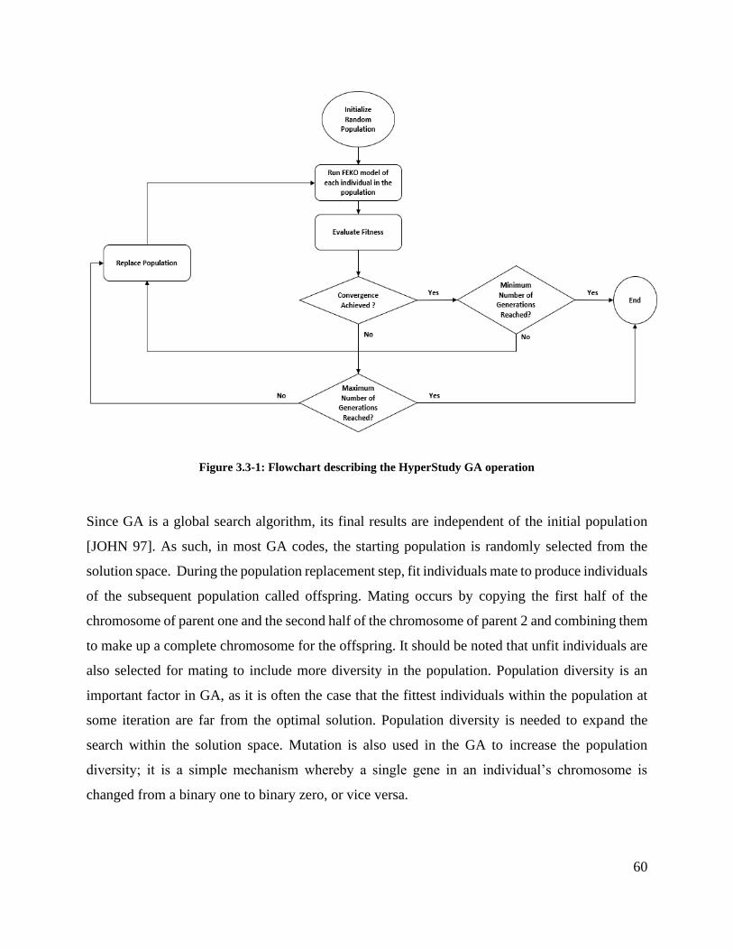
60
Figure 3.3-1: Flowchart describing the HyperStudy GA operation
Since GA is a global search algorithm, its final results are independent of the initial population
[JOHN 97]. As such, in most GA codes, the starting population is randomly selected from the
solution space. During the population replacement step, fit individuals mate to produce individuals
of the subsequent population called offspring. Mating occurs by copying the first half of the
chromosome of parent one and the second half of the chromosome of parent 2 and combining them
to make up a complete chromosome for the offspring. It should be noted that unfit individuals are
also selected for mating to include more diversity in the population. Population diversity is an
important factor in GA, as it is often the case that the fittest individuals within the population at
some iteration are far from the optimal solution. Population diversity is needed to expand the
search within the solution space. Mutation is also used in the GA to increase the population
diversity; it is a simple mechanism whereby a single gene in an individual’s chromosome is
changed from a binary one to binary zero, or vice versa.

61
Linearly Polarized Microstrip Patches: H-Plane Coupling
Goals
In this section, a simple antenna configuration is shaped in order to achieve low mutual coupling
while maintaining the return loss levels. Figure 3.4-1 shows the initial antenna arrangement before
the shaping. This configuration is comprised of two patch antennas intended to operate within the
ISM band with a center frequency 𝑓0 = 5.7 GHz and a bandwidth of 300 MHz. The antennas are
placed along the x-axis and a decoupling surface is inserted between them. An infinite substrate
and ground plane are used in the FEKO model with 휀𝑟 = 4.5, tan(𝛿) = 0.0037, and a thickness of
1.57 mm. Since the microstrip antennas are positioned collinearly along the H-plane we will refer
to this as the H-plane co-planar coupling case, this is to follow the terminology used in similar
works in the literature [BALA 16], [YANG 03]. The antenna arrangement is geometrically
symmetrical about the yz-plane, and therefore 𝑆11 = 𝑆22. Since the materials used are isotropic
𝑆12 = 𝑆21. Hence, we will only consider 𝑆11 and 𝑆12 to capture the return loss and mutual coupling
of the antennas.
Figure 3.4-1: Unshaped MEA (mother structure)

62
Single Probe-fed Microstrip Patch
The first step in this study is to analyze the properties of a single microstrip patch antenna, which
is placed on an infinite substrate. This patch was designed using the cavity model approximation
[BALA 16] to obtain the initial length, width and probe feed location. The same parameters were
then “tuned” using FEKO modeling to arrive at the microstrip antenna shown in Figure 3.4-2. The
diameter of the feed probe is 0.8 mm.
Figure 3.4-2: Dimensions of a single probe-fed microstrip patch antenna
We begin the numerical experiment by examining the properties of the single antenna’s reflection
coefficient in addition to the far-field radiation pattern.
Figure 3.4-3: Computed reflection coefficient for the single patch antenna in Figure 3.4-2

63
Figure 3.4-4: Computed total directivity patterns for a single antenna at 5.7 GHz. The pattern coordinate
system is shown in Fig 3.4-1, and defines angle ϕ.
Figure 3.4-3 and Figure 3.4-4 show that the single microstrip patch antenna has good properties
considering that pin-fed microstrip antennas offer a bandwidth of 2%-5% [POZA 92]. Given that
a reflection coefficient value of even -6 dB is acceptable for mobile communication applications
[REHM 18] the bandwidth of this patch antenna is 5.3%.
MEA consisting of two microstrip patch antennas
Having examined an isolated single antenna, we add a second one shifted by 8.9 mm (0.17𝜆0) as
shown in Figure 3.4-5. This will establish the microstrip antenna’s performance as an element of
MEA, when there is no decoupling method applied between the MEA elements.

64
Figure 3.4-5:Dimensions of MEA design
Figure 3.4-6 shows the simulated results for the geometry in Figure 3.4-5. The values of 𝑆11 are
below −5 dB across the entire bandwidth while the mutual coupling is lower than −12 dB. In
Figure 3.4-7, we see a diagram of the surface current on the structure when port 1 is excited and
port 2 terminated with a matched load. The magnitude of the induced surface current density at
the location of port#2 is about 12 dB below that at the driven port#1. Having an induced current
on the load-terminated antenna is an undesired result of mutual coupling which we hope to reduce
using shape synthesis. We aim to reduce the mutual coupling across the 300 MHz bandwidth from
5.55 GHz to 5.85 GHz.

65
Figure 3.4-6: Computed S-parameter plot for MEA
Figure 3.4-7: Surface current density for MEA at 5.7 GHz
To ensure that the microstrip patch remains functional as antenna we will also consider the
radiation pattern when the second patch is added to the geometry. Figure 3.4-8 shows the far-field
pattern when antenna 1 is excited and antenna 2 terminated in a matched load. Comparing this far-
field pattern to the pattern of a single antenna shown in Figure 3.4-4, we note that in the 𝜙 = 0 cut

66
(xz-plane) the pattern is slightly skewed towards antenna 2, with the maximum directivity D(θ =
300, ϕ = 00) = 5 dBi. We will aim to correct this tilt in the peak directivity by using the shape
synthesis process to have the peak point back in the broadside direction.
Figure 3.4-8: Computed total directivity patterns of antenna 1, when antenna 2 is terminated in a matched
load, at 5.7 GHz.
Insertion of an unshaped decoupling surface
An unshaped decoupling surface (DS) was placed in between the antennas as shown in Figure
3.4-9. Thus maintaining the original separation distance between the antennas. As expected, we
notice some change in the S-parameter plots of the antennas now shown in Figure 3.4-10 compared
to that in Figure 3.4-6. The 𝑆11 values where the lowest value deteriorated slightly, but the mutual
coupling 𝑆12 was reduced by 4 dB to less than −16 dB. This reduction is an expected result of
adding the DS surface, which is that it acts as a “shield” between the antennas’ radiating edges.

67
Figure 3.4-9: Dimensions of MEA after introducing the DS.
Figure 3.4-10: Computed S-parameter plots after the DS is introduced

68
The reduction in coupling is also reflected in Figure 3.4-11 which shows a reduction in the induced
surface currents on the terminated antenna. In the absence of the DS, we saw that the maximum
induced current on antenna 2 was about 8 dBA/m, this was reduced to about 4 dBA/m after the
introduction of the DS. Additionally, we note that the portions of the DS closest to the exited
antenna, are more strongly excited than the rest of the DS. This is due to the geometric proximity
of the DS to the excited antenna. The magnitude of the induced surface current density at the
location of port#2 is about 18 dB below that at location of port#1, after the introduction of the DS
(compared to 12 dB without the DS).
Figure 3.4-11: Surface current density of MEA with DS, with antenna 1 excited and antenna 2 terminated
with a matched load, at 5.7 GHz.
From Figure 3.4-12 we see that the introduction of the DS tilts the far-field pattern (in the xz-
plane) more severely than, and in a direction opposite to that in, Figure 3.4-8, although the
maximum value of total directivity remains 5 dBi. This pattern “skewing” is due to the presence
of induced currents on both the terminated radiating element and the unshaped DS.

69
Figure 3.4-12: Computed total directivity patterns at 5.7 GHz, when antenna 1 is excited, with the unshaped
DS present.
Application of Shape Synthesis
We aim to minimize the mutual coupling and return loss levels by shape synthesizing not only
the decoupling surface but also the two antennas. The main goal of the shape synthesis is to
reduce 𝑆12, and adjust the magnitude and direction of the peak directivity in the far-field. The far-
field pattern skewing will be corrected in the shaping process through introducing constraints. The
constraints do not alter the objective function expression. Instead, individuals in a population (at
each iteration of the GA) that do not satisfy the constraint are effectively assigned very-high
objective function values. For example, in this case, the constraint was set such that the peak
directivity must be at least 5 dBi and occur within +/- 10 degrees of broadside. The GA will thus
work to minimize the objective function defined via the S-parameter masks while ensuring that
the above directivity pattern constraint is not violated. If an individual in a population has “good”
S-parameter properties but violates the constraint, it will be deemed unfeasible by the GA. This is
not to say that such individuals will be disqualified from being passed on to the next generations;
although such shapes (individuals) will not be considered optimum solutions in the overall process,
some of their chromosomes might still be passed on to next generations. Implementing constraints
in this manner offers flexibility in the shape synthesis process as it allows the designer to eliminate
undesired characteristics and thereby have greater control over the final solution. However, as with

70
any optimization process, one should be careful to not impose constraints that are not physically
possible. Imposing too many constraints can also shrink the solution space of feasible shapes. A
reduced solution space could ultimately prevent the shaping process from arriving at a shape that
meets the fitness criteria. The far-field directivity pattern of the two antennas and DS at the center
frequency (𝑓0 = 5.7 GHz) was simulated in FEKO and was passed to HyperStudy as a string of
36 values (𝑎1, 𝑎2, … , 𝑎36). Each magnitude value corresponds to a value in theta ranging from
−90𝑜 to 90𝑜 in increments of 5𝑜. If the maximum directivity value 𝑚𝑎𝑥(𝑎1, 𝑎2…𝑎36) is
not 𝑎16, 𝑎17, 𝑎18, 𝑎19, or 𝑎20 which corresponds to the values measured at −10𝑜 , −5𝑜 , 0𝑜 , 5𝑜 , and
10𝑜 then the peak directivity is not pointing in broadside and the shape (individual) is considered
“not feasible”. Similarly, if 𝑚𝑎𝑥(𝑎1, 𝑎2…𝑎36) < 5 dBi the shape will be considered not feasible.
The S-parameter masks for the present “H-plane coupling” case is shown in Figure 3.4-13.
Although the associated objective function is written in general form in section 3.2, for clarity we
repeat it here for this specific case:
We begin by defining the error contribution terms as shown below27:
𝑒11(𝑓𝑞) = |𝑆11(𝑓𝑞)|
𝑑𝐵− | − 5|𝑑𝐵 𝑖𝑓 |𝑆11(𝑓𝑞)|
𝑑𝐵− | − 5|𝑑𝐵 < 0
𝐴0 𝑂𝑡ℎ𝑒𝑟𝑤𝑖𝑠𝑒
( 3.4-1 )
and
27 Note that we are merely “asking” the shaping process to maintain the S11 performance and not improve it. The
“mask” value for S11 was selected to be flat with a relatively high maximum value in order to simplify this introductory
example and focus all of the optimization efforts on reducing S12.

71
𝑒12(𝑓𝑞)
=
|𝑆12(𝑓𝑞)|
𝑑𝐵− |−20|𝑑𝐵 𝑖𝑓 |𝑆12(𝑓𝑞)|
𝑑𝐵− | − 20|𝑑𝐵 < 0 𝑓𝑜𝑟 5.55 𝐺𝐻𝑧 ≤ 𝑓𝑞 < 5.65 𝐺𝐻𝑧
0 𝑂𝑡ℎ𝑒𝑟𝑤𝑖𝑠𝑒 𝑓𝑜𝑟 5.55 𝐺𝐻𝑧 ≤ 𝑓𝑞 < 5.65 𝐺𝐻𝑧
𝐴
|𝑆12(𝑓𝑞)|𝑑𝐵− |−25|𝑑𝐵 𝑖𝑓 |𝑆12(𝑓𝑞)|
𝑑𝐵− | − 25|𝑑𝐵 < 0 𝑓𝑜𝑟 5.65 𝐺𝐻𝑧 ≤ 𝑓𝑞 < 5.75 𝐺𝐻𝑧
0 𝑂𝑡ℎ𝑒𝑟𝑤𝑖𝑠𝑒 𝑓𝑜𝑟 5.55 𝐺𝐻𝑧 ≤ 𝑓𝑞 < 5.65 𝐺𝐻𝑧 0
|𝑆12(𝑓𝑞)|𝑑𝐵− |−20|𝑑𝐵 𝑖𝑓 |𝑆12(𝑓𝑞)|
𝑑𝐵− | − 20|𝑑𝐵 < 0 𝑓𝑜𝑟 5.75 𝐺𝐻𝑧 ≤ 𝑓𝑞 < 5.85 𝐺𝐻𝑧
0 𝑂𝑡ℎ𝑒𝑟𝑤𝑖𝑠𝑒 𝑓𝑜𝑟 5.55 𝐺𝐻𝑧 ≤ 𝑓𝑞 < 5.65 𝐺𝐻𝑧
( 3.4-2 )
Figure 3.4-13: Selected masks for S11 and S12
Finally, as explained in section 3.2, we combine the error contribution terms into a single
expression, which will define the fitness function of the shaping process using 13 frequency points
over the band 5.55 GHz – 5.85 GHz. By evaluating the difficulty and importance associated with
achieving the design objectives for this numerical experiment, we found that the ideal weights for
the weighting terms of this objective function to be 0.45 and 0.55. These weighting values allow
the shaping process to meet both requirements formulated in the objective function.
𝐹𝑂𝑏𝑗(𝑓) = 0.45∑|𝑒11(𝑓𝑞)|2
13
𝑞=1
+ 0.55∑|𝑒12(𝑓𝑞)|2
13
𝑞=1
( 3.4-3 )

72
Figure 3.4-14 shows the starting geometry (which will be shaped) divided into pixels28. To ensure
left/right symmetry is retained for all shapes that are synthesized, we made sure that each single
optimization bit (gene) only controls two pixels which are mirrored reflections of each other about
the yz-plane. For example, in Figure 3.4-14, only a single bit is set to zero with all the remaining
variables in the chromosome are set to 1. Yet corresponding cells are removed on either side. Note
that two of the pixels (are on either side) are larger than others. The reason is that these are points
on the geometry where the probe-feeds are attached to the patches. FEKO plants special attachment
expansion functions there. It may not fall at the intersection of two pixels, and so in this case the
two pixels in question were simply enlarged to encompass the feed points.
Figure 3.4-14: Symmetry enforced on the pixelated shape of the MEA to be shaped.
Figure 3.4-15 shows the objective function value of the fittest shape in each shaping. Significant
reductions are achieved in the first few iterations. As the iterations progress the room for
improvement decreases due to the governing physics and progress is slower.
28 This is not identical to the mesh used or the computational electromagnetic analysis done by FEKO.
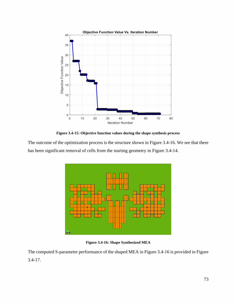
73
Figure 3.4-15: Objective function values during the shape synthesis process
The outcome of the optimization process is the structure shown in Figure 3.4-16. We see that there
has been significant removal of cells from the starting geometry in Figure 3.4-14.
Figure 3.4-16: Shape Synthesized MEA
The computed S-parameter performance of the shaped MEA in Figure 3.4-16 is provided in Figure
3.4-17.

74
Figure 3.4-17: Simulated S-parameters of shaped MEA
In order to evaluate what the shaping has achieved, we will use the result in Figure 3.4-10 as a
reference; recall that it applies to the geometry in Figure 3.4-9. We notice from Figure 3.4-17 that
S11 remains below -5 dB ( which is all we asked for via the objective function), but that the largest
S12 value has decreased by roughly 10 dB compared to Figure 3.4-10. We can also examine the
surface current diagram shown in Figure 3.4-18 to gain an insight on how the shaping process
affected the current flow from the excited port 1 to the terminated port 2. We see that there is a
significant reduction in the parasitic excitation of antenna 2. Compared to the reference model (no
DS), where the maximum surface current density on antenna 2. Recall that the magnitude of the
induced surface current density at the location of port#2 was only 12 dB below that at the driven
port#1 when there was no DS. After adding and shaping the DS, Figure 3.4-18 shows that this
difference is around 36 dB. The results presented in the surface current diagram are clearly aligned
with reduction in mutual coupling (S12) which was noted in Figure 3.4-17. As such, we can
conclude that the shaping synthesis process was successful in improving the decoupling between
the antennas. Note that the cells which are only attached through corners in the CEM model have

75
no current flowing in them, and therefore, during the fabrication process these cells must be
physically disconnected from each other.
Figure 3.4-18: Surface current density for shaped H-plane model
Figure 3.4-19 shows the pattern of the shaped MEA. We can see that the peak directivity is slightly
larger than 5dBi and lies within an angular sector centered on the broadside direction. The
constraints set on the pattern have been satisfied; the xz-plane pattern skewing recorded in Figure
3.4-8 and Figure 3.4-12 has been largely removed.
Figure 3.4-19: Computed total directivity pattern of the shaped MEA.

76
The simulated radiation efficiency plots in Figure 3.4-20 show that there is no significant change
of this metric after the shaping. We note a 10% improvement in the lower half of the bandwidth
after the shaping. In the upper half, the efficiency plots do not show any significant changes.
Figure 3.4-20: Simulated radiation efficiency before and after shaping

77
Linearly Polarized Microstrip Patches: E-Plane Coupling
Preamble
We next apply the shaping process to a case similar to that in Section 3.4, except that the two
patches are aligned along their E-plane, as shown in Figure 3.5-1. The feedpoint locations of the
antennas are on opposite sides (out-of-phase) in order to maintain symmetry. It should be noted
that the dimensions of all the elements making up the MEA arrangement in Figure 3.5-1 were
slightly altered from those used for the H-plane case. The substrate used is the same in every way
to that specified in Section 3.4.1. In Section 3.4 the shaping process was required to maintain 11S
at its unshaped value, and reduce 12S to values below a specified mask, while constraining the
total directivity pattern to have its peak within a prescribed angular sector about the broadside
direction. In the present section we add additional requirements : In addition to lowering 12S below
a prescribed mask and constraining the total directivity pattern as before, we will require the
shaping process to decrease 11S and the ECC below their unshaped values. This will be done by
adjusting the mask level for 11S and adding an ECC-term to the composite objective function. As
was done in Section 3.4, we will study this “E-plane” case in steps.
Single Microstrip Patch Reference
The computed performance of single probe-fed patch with dimensions shown in Figure 3.5-1 is
shown in Figure 3.5-2 and Figure 3.5-3, for reference. The reflection coefficient 11S of the single
patch shows acceptable properties within the frequency range 5.4 GHz to 5.7 GHz, and this will
be the frequency range of interest. Figure 3.5-3 shows the total directivity patterns with expected
maxima (5 dBi in this case, similar to Figure 3.4-4) in the broadside direction.

78
Figure 3.5-1:Dimensions of the unshaped MEA arrangement (E-plane coupling) that will form the starting
shape for the shape synthesis application.

79
Figure 3.5-2: Computed reflection coefficient of the single isolated patch antenna.
Figure 3.5-3: Computed total directivity radiation pattern of the single patch antenna in the two principal
planes. The frequency is 5.55 GHz.

80
MEA Consisting of Two Patch Antennas: E-Plane Alignment
Before proceeding to shaping, we examine the properties of the two patches shown in Figure
3.5-1 but with the unshaped DS absent. The patches are separated by 9.6. The Antenna’s combined
computed characteristics will be used as a reference and compared to the results that will be
produced through shape optimization. Figure 3.5-4 reveals that there is not a significant change in
11S compared to what it was (Figure 3.5-2) when the 2nd patch was absent. The 12S rises as high
as -12 dB; in MIMO applications [MEI 18] the coupling between any two elements should
preferably be below -20 dB.
Figure 3.5-4: Computed S-parameters of the MEA (two patches without a DS).
The surface current density when antenna 1 is excited and antenna 2 is terminated with a 50Ω load
is shown in Figure 3.5-5. The magnitude of the induced surface current density at the location of
port#2 is about 11dB below29 that at the driven port#1. The radiation pattern of antenna#1 under
29 We aim to reduce this through the shape synthesis process with a DS present.

81
the same conditions is now, as expected, skewed in the yz-plane ( 90 = plane), as is clear from
Figure 3.5-6.
Figure 3.5-5: Surface current density on the MEA(two patches and no DS) when port#1 is driven and port#2
terminated. The frequency is 5.55 GHz.
Figure 3.5-6: Computed principal plane total directivity patterns of the MEA (two patches and no DS) when
port#1 is driven and port#2 terminated. The frequency is 5.55 GHz.

82
If the antennas are intended for MIMO operation, the ECC figure of merit would be of interest.
Figure 3.5-7 shows the computed30 ECC plotted over the frequency band of interest. It is
interesting to observe, by comparing Figure 3.5-4 and Figure 3.5-7 that low mutual coupling ( 12S
) values alone are not sufficient to achieve low ECC values. In Figure 3.5-4 the highest 12S values
occur around 5.6GHz, yet the ECC value is not peaked there, but has its highest value at 5.7 GHz.
This is because the 𝑆12 only measures the coupling between the antenna ports and not the radiated
far-field coupling [SHAR 13]. This provides motivation to include explicit ECC terms in the
objective function, as we will do here31.
Figure 3.5-7: ECC for the MEA (two patches and no DS).
Although it will not be included in the objective function, we out of interest will monitor the
total active reflection coefficient32 (TARC) figure of merit in order to simply record any
enhancements in the TARC brought about by the shape synthesis process. Since the TARC is
30 This is done using the radiation patterns, as explained in Section 2.3.7.
31 The EEC is actually already sufficiently low, as the maximum value of 0.12 is still well below the 0.5 requirement
mentioned for mobile terminals. Nevertheless, we wish to explore what the shape optimization process is able to
achieve as regards further reducing the ECC.
32 Defined in Section 2.3.6.

83
calculated strictly from the S-parameters, enhancing the port isolation between the antennas should
as a consequence reduce the TARC values. For the current MEA configuration (that is, two patches
and no DS) the TARC plotted in Figure 3.5-8 shows a worst-case value of -3 dB, which is
considered high for a MIMO implementation [BROW 06]. We will see in Section 3.5.5 that adding
a DS and shaping the entire resulting MEA is able to decrease this.
Figure 3.5-8: Computed TARC for the MEA (two patches and no DS).
MEA Consisting of Two Patch Antennas and an (Unshaped) Decoupling Surface
The next step in this study, once again for later reference, is to examine the behavior of an MEA
consisting of the two patches and the unshaped DS, precisely as shown in Figure 3.5-1. Figure
3.5-9 shows that (compared to Figure 3.5-4) the location of the minimum 11S value (the
“resonance”) and the maximum 12S value has shifted from 5.6 GHz to 5.53 GHz. The presence of
the unshaped DS has detuned the antennas. From Figure 3.5-10 we see that the magnitude of the
induced surface current density at the location of port#2 is about still about 11dB below that at the
driven port#1, as it was in Figure 3.5-5. The radiation pattern of antenna#1 under the same
conditions is now that in Figure 3.5-11. Surprisingly, introduction of the unshaped DS corrected

84
the skewing of the radiation pattern in the 90 = plane that was observed (without the unshaped
DS present) in Figure 3.5-6, across the whole frequency band. The maximum total directivity has,
however, decreased to 4.3 dBi, which is less than the 5 dBi we wish to achieve in the broadside
direction. The ECC plot in Figure 3.5-12 is similar to the DS-less case in Figure 3.5-7; the
maximum ECC value has fallen to 0.10 from 0.12 with the DS present (due to a small amount of
additional isolation), but we do not attach too much significance to this.
Figure 3.5-9: Computed S-parameters of the MEA consisting of two patches and the unshaped DS.

85
Figure 3.5-10: Surface current density on the MEA consisting of two patches and the unshaped DS when
port#1 is driven and port#2 terminated. The frequency is 5.55 GHz.
Figure 3.5-11: Computed total directivity principal plane patterns of the MEA consisting of two patches and
the unshaped DS. The frequency is 5.55 GHz

86
Figure 3.5-12: Computed ECC for the MEA consisting of two patches and the unshaped DS.
3.5.5 MEA Consisting of Two Patch Antennas and a Shaped Decoupling Surface
We now apply the shaping procedure to the starting shape shown in Figure 3.5-1. The pixelated
form is that in Figure 3.5-13. Top/down symmetry will be enforced during shaping.
Figure 3.5-13: Starting Structure of E-Plane coupled MEA

87
The objective function was formulated in a similar manner to that used for the “H-plane coupling”
case in Section 3.4. The S-parameters masks were simply upper limit values of -10 dB and -20
dB for 𝑆11 ancd 𝑆12, respectively. As promised in Section 3.5.1, a new term is added to the
objective function to allow the GA to include the ECC between the pair of antennas when taking
decisions on the shapes that arise in each iteration. The 𝑒𝐸𝐶𝐶 error term can be formulated in the
same way as 𝑒11 and 𝑒12, and will be assigned an upper mask value33 of 0.05 or -13 dB over the
frequency band of interest. Thus, the objective function component error terms are
𝑒11(𝑓𝑞) = |𝑆11(𝑓𝑞)|
𝑑𝐵− |−10|𝑑𝐵 𝑖𝑓 |𝑆11(𝑓𝑞)|
𝑑𝐵− | − 10|𝑑𝐵 < 0
𝐴 0 𝑂𝑡ℎ𝑒𝑟𝑤𝑖𝑠𝑒
( 3.5-1 )
𝑒12(𝑓𝑞) = |𝑆12(𝑓𝑞)|
𝑑𝐵− |−20|𝑑𝐵 𝑖𝑓 |𝑆11(𝑓𝑞)|
𝑑𝐵− |−20|𝑑𝐵 < 0
𝐴0 𝑂𝑡ℎ𝑒𝑟𝑤𝑖𝑠𝑒
( 3.5-2 )
and
𝑒𝐸𝐶𝐶(𝑓𝑞) = |𝜌𝑒 (𝑓𝑞)|
𝑑𝐵− |−13|𝑑𝐵 𝑖𝑓 |𝜌𝑒(𝑓𝑞)|
𝑑𝐵− | − 13|𝑑𝐵 < 0
𝐴0 𝑂𝑡ℎ𝑒𝑟𝑤𝑖𝑠𝑒
( 3.5-3 )
with
𝜌𝑒|𝑑𝐵 = 10 𝑙𝑜𝑔 𝜌𝑒 ( 3.5-4 )
33 It should be noted that in the literature ECC is not often quoted in decibels; however, to formulate the objective
function we had to make the decision to convert the values to dB in order to ensure consistency since 11S and 12S are
expressed in decibels. This is because the ECC values expressed in decimal are less than 1, and when squared in the
error term, ECC will have no or negligible impact on the objective function.

88
The complete objective function is
𝐹𝑂𝑏𝑗(𝑓) = 0.55∑|𝑒11(𝑓𝑞)|2
13
𝑞=1
+ 0.35∑|𝑒12(𝑓𝑞)|2
13
𝑞=1
+ 0.1∑|𝑒𝐸𝐶𝐶(𝑓𝑞)|2
13
𝑞=1
( 3.5-5 )
In addition to minimizing 𝑆11, 𝑆12, and ECC, we constrain the total directivity pattern when port#1
is driven and port#2 is terminated to be at least 5 dBi with the peak34 in a 10 cone centered on the
broadside direction at the centre frequency 𝑓𝑜= 5.55 GHz, as was also done (and explained) in
Section 3.4.
During pilot runs for this shape optimization problem we found that minimizing 𝑆11 was
significantly harder to achieve by the GA compared to minimizing 𝑆12. We initially formulated
the objective function with equal weights on the 𝑒11 and 𝑒12 parts, but found that such weights
always caused the process to terminate without achieving the 𝑆12 and 𝑆11 goals. A larger weighting
multiplier was therefore assigned to 𝑒11, as seen in expression (3.5-5). A low weight was assigned
to the 𝑒𝐸𝐶𝐶 terms because the ECC of the starting shape was already close to the target value of -
13 dB (0.05).
The progress of the shaping process is represented by the plot of the objective function value versus
the iteration number in Figure 3.5-14. Because of the similarity of the problem to that in Section
3.4, it is not surprising that the behaviour is much like that in Figure 3.4-15. The outcome is the
shape synthesized MEA in Figure 3.4-15.
34 This is an important issue. In a session of the 18th International Symposium on Antenna Technology and Applied
Electromagnetics (ANTEM), Waterloo, Canada, August 2018, comments were made to the effect that one cannot reap
the MIMO benefits of low correlation between MEA elements if the patterns of these elements are not pointed in their
intended directions. By using the shaping process we could demand slightly different pattern peak directions for the
elements in an MEA if the system concepts require it. This would allow us to remove the geometrical symmetry that
has been enforced during the shaping process here and in Section 3.4, but 22S would need to be included in the
objective function as well since it will no longer be identical to 11S .

89
Figure 3.5-15: The MEA consisting of two patches and a DS after the shaping is completed
We see in Figure 3.4-16 that the S-parameter performance meets the mask limits specified. As
“requested”, the shaping procedure has lowered the maximum value of 11S from (the reference
case value of) -6dB to -10dB, and decreased the maximum value of 12S by 6dB so that 12S is
below -20dB over the whole band. The latter is reflected in the magnitude of the induced surface
current density at the location of port#2 (in Figure 3.4-17) which is now roughly than 21dB below
Figure 3.5-14: Objective function value during the shape optimization of the MEA consisting of two patches and DS
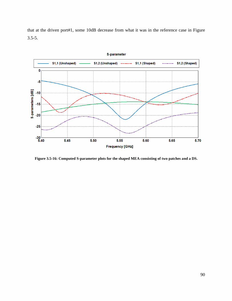
90
that at the driven port#1, some 10dB decrease from what it was in the reference case in Figure
3.5-5.
Figure 3.5-16: Computed S-parameter plots for the shaped MEA consisting of two patches and a DS.

91
Figure 3.5-17: Surface current density on the shaped MEA consisting of two patches and a DS, when port#1 is
driven and port#2 terminated. The frequency is 5.55 GHz.
The individual MEA element pattern35 is shown in Figure 3.5-18. The peak total directivity is
indeed 5 dBi, and in the 𝜙 = 900 this peak occurs about 10 off broadside instead of 30 as for
the skewed MEA with the two patches and no DS, as depicted in Figure 3.5-6. It is possible to
“draw” the peak closer to the broadside direction, but only by sacrificing some isolation. The shape
process can be used to establish such trade-offs, with the wider “design space” offered by
performing shaping instead of accepting the geometry restrictions of pre-selected geometries.
Although the ECC behaviour (for the shaped MEA) in Figure 3.5-19 is much improved compared
to the reference cases in Figure 3.5-7 and Figure 3.5-12, the ECC mask value of 0.05 has not been
satisfied36 over the complete frequency band, even though the shaping process terminated. This
could be prevented by using a larger weight in front of the ECC term in expression (3.5-5), or
lowering expectations on the other performance quantities, and so on. It became clear from many
other shaping runs that one is always trying to “play the physics”, given the starting shape (in this
case Figure 3.5-13). Another possibility would be to alter the geometry (eg. it need not be
35 Recall that the geometrical symmetry enforced during shaping
36 The ECC rises to about 0.067 at the upper end of the frequency band.

92
rectangular) of the unshaped DS to give the synthesis algorithm more conductor “to play with”.
The possibilities are endless, and could be driven by specific size constraints in some particular
application, for instance. The TARC curves in Figure 3.5-20 show a worst-case value of about -6
dB. Although TARC was not included in the objective function, we still see an improvement of
about 3 dB compared to the worst case in Figure 3.5-8. If TARC were deemed to be a more
important figure of merit than 11S it could in principle be included in the objective function37
instead of 11S .
Figure 3.5-18: Computed total directivity principal plane patterns on the shaped MEA consisting of two
patches and a DS when port#1 is driven and port#2 terminated. The frequency is 5.55 GHz.
37 The ability to use the S-parameter information to determine the TARC, as described in Section 2.3.6, and then
incorporate this in the objective function, is at present not possible in the Hyperstudy suite [HYPE 20].
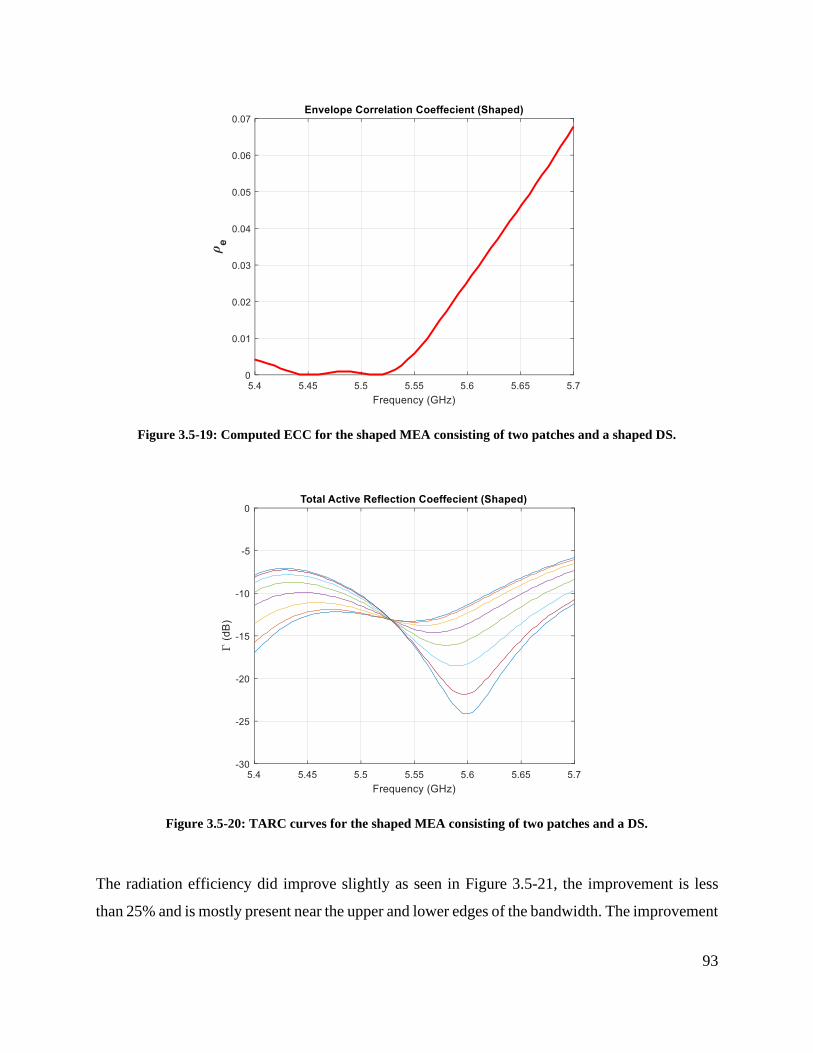
93
Figure 3.5-19: Computed ECC for the shaped MEA consisting of two patches and a shaped DS.
Figure 3.5-20: TARC curves for the shaped MEA consisting of two patches and a DS.
The radiation efficiency did improve slightly as seen in Figure 3.5-21, the improvement is less
than 25% and is mostly present near the upper and lower edges of the bandwidth. The improvement

94
in efficiency was not intended in the initial design, however as with any other antenna metric the
radiation efficiency can be included in the objective function if need be.
Figure 3.5-21: Simulated radiation efficiency plots before and after shaping two patches and DS
Patch Antenna Polarization
As discussed in sections 3.4 and 3.5, we have opted to optimize the farfield radiation patterns
based on the total directivity pattern rather than the co-polarization directivity component. The
reason for this is that MEA antennas are typically used for MIMO systems that rely on multipath
to achieve the increased channel capacity. As a result, the polarization of the signals arriving at the
antennas after traversing the multipath environment is not known and will likely be randomly
varying. Therefore, optimizing for a high co-polarization (low cross-polarization) component
would not have provided us with the complete radiation performance of the antenna for MIMO
application. Nevertheless, the cross-polarization components (Ludwig-III) were examined for both
H-plane and E-Plane cases. The cross-polarization components for the H-plane and E-plane cases
are shown in Figure 3.6-1 and Figure 3.6-2, respectively. In both cases we can see that the cross-
pol components have increased from less than -20dBi before the shaping, to about 2.5 dBi after
the shaping. These results show that the shaping process has changed the polarization of the
antennas from having vertical polarization to having 45o polarization. Since both E-plane and H-

95
plane cases are symmetrical, the polarizations of antenna #1 and antenna #2 will point in opposite
directions after the shaping is completed. The results in this section demonstrate that global search
algorithm for the shaping process forced the antennas to have orthogonal polarizations to meet the
requirements set in the objective function.
Figure 3.6-1: Computed cross-polarization directivity components in the farfield for two antennas and DS
before and after shaping (H-plane case)
Figure 3.6-2: Computed cross-polarization directivity components in the farfield for two antennas and DS
before and after shaping (E-plane case)

96
Concluding Remarks
In this chapter, we described the shape synthesis process. This included the decision flowchart
of the genetic algorithm that controls the shape synthesis process. Importantly, the construction of
the objective functions, which is key to the success of the shape optimisation, was discussed at
length in Sections 3.2, 3.4.5 and 3.5.5. Two examples of the application of shape synthesis in the
design of decoupling surfaces were presented. Both examples involved probe-fed microstrip patch
antennas separated by a decoupling surface located on the same plane as the patches. To
demonstrate the effectiveness of the shape synthesis algorithm, the examples were purposefully
selected so that the patches were closely spaced along their common H-plane and common E-
plane, respectively.
In the first example (“H-plane” case in Section 3.4) we initially concentrated on reducing mutual
coupling (S12 = S12) while preserving the input reflection coefficients (S11 = S22) through
incorporating these in the objective function, and shaping both the decoupling surface and the
patches. It was observed (even without shaping or without the decoupling surface) that there is a
tilt in the far-field directivity pattern in the 𝜙 = 00 cut. To rectify this tilt, we introduced an
additional term in the optimizer’s software tool to “pin” the peak directivity on broadside. The
final result produced by the shape synthesis process showed that we were able to reduce the mutual
coupling from -16 dB to less than -25 dB and correct the tilt in the far-field directivity pattern. In
the second example (“E-plane” case in Section 3.5) we were successful in showing the flexibility
of the shaping process by including yet additional goals in the objective function. This enabled us
to not only reduce Sii and Sij, but also directly the ECC, all the while preserving the value and
direction of the maximum directivity of the individual patches that would have otherwise (without
shaping) been tilted in the 𝜙 = 900 cut. Through the shape synthesis process, we were able to
reduce the 𝑆𝑖𝑖, 𝑆𝑖𝑗, and ECC by 6 dB, 6 dB, and 50% respectively. As far as the author is aware,
this is the first time that shape synthesis has been used for the automated shaping of an MEA
system with a decoupling surface.

97
Chapter 4 The Shape Synthesis of Non-Coplanar Decoupling
Surfaces
Preliminary Remarks
In Chapter 3, we explored how shape synthesis can be used as a method to decouple closely
packed antennas, with the antennas and the decoupling structures lying on the same plane
(‘coplanar’). We demonstrated the flexibility of this method by incorporating several performance
goals in the objective function. In the present chapter, our aim is to further demonstrate, also for
the first time, the use of shape synthesis for an antenna arrangement where the decoupling surface
(DS) is not located in the same plane as the antenna elements proper (‘non-coplanar’). The MEA
system is extended to one consisting of four elements (albeit still probe-fed patches) that lie in a
single plane.
The MEA system, without a DS, is introduced in Section 4.3 and its performance parameters (Sij,
TARC, ECC and radiation patterns) computed. These serve as a reference for the performance
achieved when a DS is later added. In Section 4.4 a DS is introduced into the MEA system (still
consisting of four elements), consisting of an unshaped rectangular conducting plate located above
(not in the same plane as) the four rectangular patch elements. The performance parameters are
again computed and, as expected when one simply “invades” a radiating structure by inserting an
additional piece of conductor, all are degraded. In Section 4.6 the shape synthesis process is applied
to this structure by the shaping of the DS, utilising an objective function defined in Section 4.5.
The contrast between the performance with the shaped DS and those in Section 4.3 (no DS) and
Section 4.4 (unshaped DS) are very satisfactory indeed. Section 4.7 concludes the chapter.
Single Probe-Fed Microstrip Patch
The shape synthesis process used in this chapter is similar to that developed in Chapter 3.
However, since we are dealing with a four-element MEA system, there are some adjustments
which have to be made on the fitness function side to account for the additional S-parameters
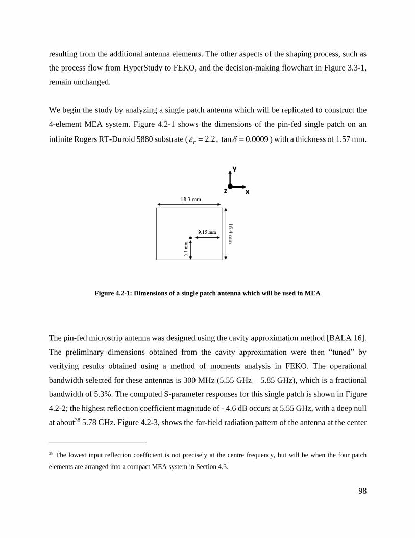
98
resulting from the additional antenna elements. The other aspects of the shaping process, such as
the process flow from HyperStudy to FEKO, and the decision-making flowchart in Figure 3.3-1,
remain unchanged.
We begin the study by analyzing a single patch antenna which will be replicated to construct the
4-element MEA system. Figure 4.2-1 shows the dimensions of the pin-fed single patch on an
infinite Rogers RT-Duroid 5880 substrate ( 2.2r = , tan 0.0009 = ) with a thickness of 1.57 mm.
Figure 4.2-1: Dimensions of a single patch antenna which will be used in MEA
The pin-fed microstrip antenna was designed using the cavity approximation method [BALA 16].
The preliminary dimensions obtained from the cavity approximation were then “tuned” by
verifying results obtained using a method of moments analysis in FEKO. The operational
bandwidth selected for these antennas is 300 MHz (5.55 GHz – 5.85 GHz), which is a fractional
bandwidth of 5.3%. The computed S-parameter responses for this single patch is shown in Figure
4.2-2; the highest reflection coefficient magnitude of - 4.6 dB occurs at 5.55 GHz, with a deep null
at about38 5.78 GHz. Figure 4.2-3, shows the far-field radiation pattern of the antenna at the center
38 The lowest input reflection coefficient is not precisely at the centre frequency, but will be when the four patch
elements are arranged into a compact MEA system in Section 4.3.
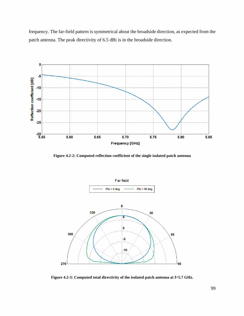
99
frequency. The far-field pattern is symmetrical about the broadside direction, as expected from the
patch antenna. The peak directivity of 6.5 dBi is in the broadside direction.
Figure 4.2-2: Computed reflection coefficient of the single isolated patch antenna
Figure 4.2-3: Computed total directivity of the isolated patch antenna at f=5.7 GHz.

100
MEA System Consisting of Four Patch Antennas
After validating the results for the single patch antenna, we introduce three additional yet
identical antennas that are placed an equal distance from each other. Figure 4.3-1 shows the layout
and dimensions of this 4-element MEA system. The antennas are equidistant from each other to
maintain symmetry about the vertical and horizontal axes. The antennas are mirrored about the
axes and separated by 7.6 mm or 0.14𝜆0. The design was forced to be symmetric to simplify the
shaping process as will be discussed in the following sections.
Figure 4.3-1: Dimension of MEA consisting of four patch antennas
Similar to the situation in Chapter 3, due to the symmetric nature of this design and the isotropic
nature of the materials, many of the S-parameters are equal to each other. As such, we can focus

101
on examining a subset of the S-parameters when studying the S-parameter response of this MEA
system. The equivalences are as follows:
• S11 = S33 = S22 = S44
• S12 = S21 = S34 = S43
• S13 = S42 = S24 = S31
• S14 = S23 = S32 = S41
For simplicity, we will only examine four S-parameters (S11, S12, S13, and S14) since they capture
all the information needed to evaluate the S-parameter properties of this model. Figure 4.3-2 shows
the S-parameter response for the four antennas. We note that there is a slight improvement in the
reflection coefficient (S11) where the maximum value is now 0.5 dB lower compared to the single
antenna case in Figure 4.2-2. The highest coupling magnitude is 𝑆12 which is between the
horizontally adjacent antennas #1 and #2, where the maximum value is -15 dB. The coupling
coefficients for vertically adjacent antennas, 𝑆13, also shows a plot with values which is similar to
𝑆12. These are expected results since the horizontally and vertically adjacent elements are
geometrically closer to each other than the diagonal elements pairs. Nonetheless, these coupling
values are still significantly higher than the -20 dB mutual coupling requirement for MIMO
applications [MEI 18].
Figure 4.3-2: Computed S-parameters of the MEA (four patches without DS).

102
Figure 4.3-3 shows the surface currents on the model when antenna#1 is excited while the
remaining three antennas are terminated with a 50 Ohm load. We can see that there are induced
surface currents on the non-excited antennas due to coupling. The induced currents are highest on
antenna#2; at the location of port#2 has an induced current which is 9 dB lower than that at port#1.
At the location of ports #3 and #4 the induced surface currents are 18 dB lower than that at port#1.
Figure 4.3-3: Surface current density on the MEA (four patches and no DS) when port#1 is driven, and the
remaining ports are terminated. The frequency is 5.7 GHz.
Figure 4.3-3 shows the far-field radiation pattern of antenna#1 while the remaining antennas are
terminated. The mutual coupling between antenna#1 and the remaining antennas has slightly
deformed the radiation pattern. Compared to the isolated patch case in Figure 4.2-3, we see that
Figure 4.3-4 shows the peak of the pattern is no longer pointing to broadside. We also note a slight
decrease of 1.5 dB in the peak directivity; this is especially clear in the 𝜙 = 900 cut. However,
there is no significant change noted with respect to the beam-width of the patterns.
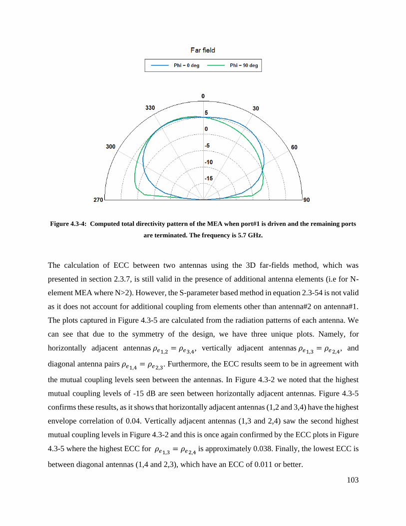
103
Figure 4.3-4: Computed total directivity pattern of the MEA when port#1 is driven and the remaining ports
are terminated. The frequency is 5.7 GHz.
The calculation of ECC between two antennas using the 3D far-fields method, which was
presented in section 2.3.7, is still valid in the presence of additional antenna elements (i.e for N-
element MEA where N>2). However, the S-parameter based method in equation 2.3-54 is not valid
as it does not account for additional coupling from elements other than antenna#2 on antenna#1.
The plots captured in Figure 4.3-5 are calculated from the radiation patterns of each antenna. We
can see that due to the symmetry of the design, we have three unique plots. Namely, for
horizontally adjacent antennas 𝜌𝑒1,2 = 𝜌𝑒3,4, vertically adjacent antennas 𝜌𝑒1,3 = 𝜌𝑒2,4, and
diagonal antenna pairs 𝜌𝑒1,4 = 𝜌𝑒2,3. Furthermore, the ECC results seem to be in agreement with
the mutual coupling levels seen between the antennas. In Figure 4.3-2 we noted that the highest
mutual coupling levels of -15 dB are seen between horizontally adjacent antennas. Figure 4.3-5
confirms these results, as it shows that horizontally adjacent antennas (1,2 and 3,4) have the highest
envelope correlation of 0.04. Vertically adjacent antennas (1,3 and 2,4) saw the second highest
mutual coupling levels in Figure 4.3-2 and this is once again confirmed by the ECC plots in Figure
4.3-5 where the highest ECC for 𝜌𝑒1,3 = 𝜌𝑒2,4 is approximately 0.038. Finally, the lowest ECC is
between diagonal antennas (1,4 and 2,3), which have an ECC of 0.011 or better.
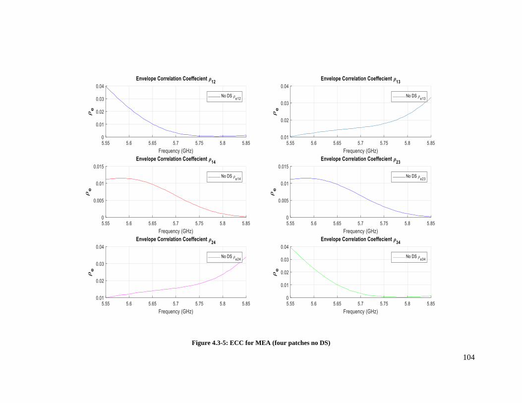
104
Figure 4.3-5: ECC for MEA (four patches no DS)
105
The specific expression for the TARC of a four-element MEA is slightly different compared to
that of the 2-element MEA written down in Section 2.3.6. Starting from the general defination for
TARC provided in expression (2.3-33), namely
Γ𝑎𝑡 = √
∑ |𝑏𝑖|2𝑁𝑖=1
∑ |𝑎𝑖|2𝑁𝑖=1
( 4.3-1 )
the relation
𝒃 = 𝑺𝒂 ( 4.3-2 )
for the 4-element case becomes
[
𝑏1𝑏2𝑏3𝑏4
] = [
𝑆11 𝑆12 𝑆13 𝑆14𝑆21 𝑆22 𝑆23 𝑆24𝑆31𝑆41
𝑆32𝑆42
𝑆33𝑆43
𝑆34𝑆44
] [
𝑎1𝑎2𝑎3𝑎4
] ( 4.3-3 )
Defining 𝑎1 = 𝑎0𝑒𝑗0 as the reference excitation phase and amplitude; we can define the
excitations of the remaining three antennas as having the same amplitude as well as a phase shift
relative to 𝑎1.
[
𝑎1𝑎2𝑎3𝑎4
]=
[ 𝑎0
𝑎0𝑒𝑗1
𝑎0𝑒𝑗2
𝑎0𝑒𝑗3]
( 4.3-4 )
The system of equations can then be expanded to:
𝑏1 = 𝑎0(𝑆11 + 𝑆12𝑒𝑗1 + 𝑆13𝑒
𝑗2 + 𝑆14𝑒𝑗3) ( 4.3-5 )
𝑏2 = 𝑎0(𝑆21 + 𝑆22𝑒𝑗1 + 𝑆23𝑒
𝑗2 + 𝑆24𝑒𝑗3) ( 4.3-6 )
𝑏3 = 𝑎0(𝑆31 + 𝑆32𝑒𝑗1 + 𝑆33𝑒
𝑗2 + 𝑆34𝑒𝑗3) ( 4.3-7 )

106
𝑏4 = 𝑎0(𝑆41 + 𝑆42𝑒𝑗1 + 𝑆43𝑒
𝑗2 + 𝑆44𝑒𝑗3) ( 4.3-8 )
finally,
Γ𝑎𝑡 = √
𝑎02 (𝑏1
2 + 𝑏22 + 𝑏3
2 + 𝑏42)
4 𝑎02 ( 4.3-9 )
Capturing all possible variations between the variable phases will be difficult. So we will only
consider a subset of plots by keeping one psi variable constant and changing the other two psi’s in
steps of 45o. For example, Figure 4.3-6 shows the TARC curves calculated when 1 is kept
constant39 while 2,
3 are varied from 0o to 180o in steps of 45o. Figure 4.3-6 captures the TARC
when excitation signals have constant phase between antenna#1 and antenna#2 and when antennas
#3 and #4 have excitition signals with changing phase. The worst-case TARC in this scenario is
less than -6 dB, which is acceptable.
39 In this context, the constant phase is fixed to 0o. Note that in all cases 0 which corresponds to antenna#1 is
always fixed to 0o.

107
Figure 4.3-6: TARC of MEA consisting of 4 patch antennas and no DS. These plots are taken when Antenna
#1 and #2 have constant phase, while antenna #3 and #4 have a varying phase.
Figure 4.3-7: TARC of MEA consisting of 4 patch antennas and no DS. These plots are taken when Antenna
#1 and #3 have constant phase, while antenna #2 and #4 have a varying phase.

108
Figure 4.3-8: TARC of MEA consisting of 4 patch antennas and no DS. These plots are taken when Antenna
#1 and #4 have constant phase, while antenna #2 and #3 have a varying phase.
In all three TARC scenarios presented above, Figure 4.3-7 shows that the worst TARC case is
when antennas #1 and #3 are kept in phase while varying the phases for antennas #2 and #4.
Particularly, this happens when antennas #2 and #4 are both 180o or completely out of phase with
antennas #1 and #3. The TARC values in all scenarios are acceptable as they are close to the -6 dB
requirement for MIMO, with the exception of scenario 2 in Figure 4.3-7 where the worst case plot
is consistently greater than -6 dB [SHAR 13].
The 4-Element MEA & an Unshaped Decoupling Surface
Having established the benchmark performance of the 4-element antenna as MIMO antenna in
section 4.3, we can introduce the non-coplanar decoupling surface. Figure 4.4-1 below shows the
added decoupling surface which is printed on the same substrate material as the microstrip
antennas RT-Duroid 5880 (thickness 1.57 mm). The substrate containing the DS is raised 20 mm
above the antennas (along the normal axis), the DS is pixelated in 3.5 mm square cells. The 20
mm distance of separation between the antennas and DS was slected as such in order for the DS
to be suffeciently close to the antennas so that any changes on the DS shape would have an impact

109
on the antennas S-parameters. The copper-backing on the board removed in order to allow for
proper far-field transmission and decoupling40 of the antennas. The DS is divided into small cells
for shaping, as was done in Chapter 3, the dimensions are shown in Figure 4.4-2. To limit the
number of variables controlling the shaping process, we have chosen to only shape the DS.
Figure 4.4-1: Top and Iso view of the MEA after introducing the DS
Figure 4.4-2: Dimensions of the DS
The S-parameter plots after introducing the DS are shown in Figure 4.4-3. We can see that all the
reflection and mutual coupling coefficients (S12) deteriorate significantly. The maximum value for
40 Decoupling will not occur until after the DS is shaped.

110
𝑆11 is now over -5 dB in the upper frequencies. 𝑆14 shows significant increase with a maximum
value of -6 dB after introducing the DS. This is due to the effect of the unshaped DS acting as
reflector in close proximity to the antennas.
Figure 4.4-3: Computed S-parameter plots of the MEA consisting of four patches and the unshaped DS.
The introduction of the DS also deforms the far-field radiation pattern of antenna#1 as seen in
Figure 4.4-4, since the unshaped decoupling surface is a sheet of copper the radiation pattern is
reflected which causes deformation in the pattern. The setup and results here show that the far-
fields are transmitted in the direction parallel to the antennas and the DS, thus resembling the far-
field behaviour of waveguide antenna without the sidewalls.

111
Figure 4.4-4: Computed total directivity pattern of the MEA consisting of four patches and the unshaped DS,
when port#1 is driven and remaining ports are terminated. The frequency is 5.7 GHz
Figure 4.4-5: Surface current on DS when port#1 is driven and the remaining ports are terminated. The
frequency is 5.7 GHz

112
Figure 4.4-6: Surface current on the MEA when port#1 is driven and the remaining ports are terminated.
The frequency is 5.7 GHz.
Figure 4.4-5 and Figure 4.4-6 show the surface currents on the structure when antenna#1 is excited
while the remaining antennas are terminated. There is a significant increase of 9 dB for the induced
surface currents on antennas #2, #3 and #4. Prior to introducing the DS, Figure 4.3-3 was showing
that the current at port#2 was 9 dB lower than that at port#1; after introducing the unshaped DS,
the induced current at port#2 is roughly equal to that at port#1. This validates the results seen in
the S-parameter where there was a significant increase in the coupling after introducing the DS
into this model. However, such a result is expected since the DS is constructed from copper, which
reflects any incoming waves from antenna #1 (excited) back to the terminated antennas causing
an increase in the induced currents on the surfaces of neighboring antennas, thus increasing the
magnitude of induced currents.
Objective Function Used in the Shape Synthesis Process The objective function for this numerical experiment was formulated with the following goals:
To reduce the coupling between all antenna elements (𝑆12, 𝑆13, 𝑆14) to a value of -20 dB or lower.
To maintain the reflection coefficient at less than -5 dB.
To ensure the total directivity peak in the far-field is no less than 5 dBi and points within +/- 5o
of broadside.

113
One of the difficulties faced when completing this numerical experiment was the computation
duration needed to complete a full-wave analysis of the model and evaluate the fitness function.
The reason for the extended computation time is the large design footprint combined with a fine
moment method meshing and a more sophisticated fitness function. In order to reduce the
computational cost of this experiment, we opted not to include the ECC in the objective function,
as this value was sufficiently low in the starting mother structure (without DS). Additionally, we
chose to enforce left/right and up/down symmetry on the DS41. This was achieved by configuring
a single binary bit (gene) to control retention/removal of four cells that are mirrored across the
axes. Figure 4.5-1 shows an example where a single binary bit was set to zero whilst the remaining
variables are set to one.
Figure 4.5-1: Symmetry is retained after removal of cells in the DS
To achieve the optimization goals for this section, we can formulate the objective function for the
reflection coefficient value as follows42:
41 No pixelization was performed on the actual antenna elements since we do not plan to shape them.
42 Note that we are once again merely asking the shape synthesizer to maintain the reflection coefficient at -5 dB and
not improve it.

114
𝑒11(𝑓𝑞) = |𝑆11(𝑓𝑞)|
𝑑𝐵− |−5|𝑑𝐵 𝑖𝑓 |𝑆11(𝑓𝑞)|
𝑑𝐵− |−5|𝑑𝐵 < 0
𝑘𝑘𝑘𝑘𝑘𝑘𝐴0 𝑂𝑡ℎ𝑒𝑟𝑤𝑖𝑠𝑒
( 4.5-1 )
The mutual coupling requirements can be encoded into the objective function:
𝑒12(𝑓𝑞) = |𝑆12(𝑓𝑞)|
𝑑𝐵− |−20|𝑑𝐵 𝑖𝑓 |𝑆12(𝑓𝑞)|
𝑑𝐵− | − 20|𝑑𝐵 < 0
𝐴0 𝑂𝑡ℎ𝑒𝑟𝑤𝑖𝑠𝑒
( 4.5-2 )
𝑒13(𝑓𝑞) = |𝑆13(𝑓𝑞)|
𝑑𝐵− |−20|𝑑𝐵 𝑖𝑓 |𝑆13(𝑓𝑞)|
𝑑𝐵− | − 20|𝑑𝐵 < 0
𝐴0 𝑂𝑡ℎ𝑒𝑟𝑤𝑖𝑠𝑒
( 4.5-3 )
𝑒14(𝑓𝑞) = |𝑆14(𝑓𝑞)|
𝑑𝐵− |−20|𝑑𝐵 𝑖𝑓 |𝑆14(𝑓𝑞)|
𝑑𝐵− |−20|𝑑𝐵 < 0
𝐴0 𝑂𝑡ℎ𝑒𝑟𝑤𝑖𝑠𝑒
( 4.5-4 )
After selecting the appropriate weights for each error term, we can combine these terms into a
single function.
𝐹𝑂𝑏𝑗(𝑓) = 0.35∑|𝑒11(𝑓𝑞)|2
13
𝑞=1
+ 0.3∑|𝑒12(𝑓𝑞)|2
13
𝑞=1
+ 0.2∑|𝑒13(𝑓𝑞)|2
13
𝑞=1
+ 0.15∑|𝑒14(𝑓𝑞)|2
13
𝑞=1
( 4.5-5 )
To apply the far-field pattern requirement, we enforced a constraint on the far-field results for the
function similar to what was done in Section 3.5. Figure 4.5-2 shows the objective function value
during each iteration. We can see a big drop after the first iteration; this is because, as discussed
earlier in this chapter, after adding the unshaped DS the S-parameter and radiation pattern plots
were very far from meeting the objectives defined, and so there was a lot of room for rapid
improvement. In the subsequent iterations, as the objective values approach the set values, the

115
improvements get less and less significant. The objective function values finally plateau at the
110th iteration.
Figure 4.5-2: Objective function value during the shape synthesis of the MEA consisting of four patches and a
DS.
Shape Synthesis Results
The optimum result from the shape synthesis process is shown in Figure 4.6-1. Symmetry is
retained about the vertical and horizontal axes. No changes or shaping was done on the actual
antennas that reside in the bottom board of this model.
Figure 4.6-1: DS after the shaping process

116
In Figure 4.6-2 the S-parameter plots are shown after the shaping process is completed. The
reflection coefficient 𝑆11 has been maintained and is still better than the -5 dB requirement. The
mutual coupling S-parameters 𝑆12, 𝑆13, 𝑆14 show improved isolation between the antenna
elements. Prior to introducing the DS, in the reference model, 𝑆12 and 𝑆13 showed a maximum
value of -15 dB. These values have been reduced to -20 dB or better. Similarly, 𝑆14 in the reference
model had a maximum value of -20 dB; after shaping the DS this reduced to -22.5 dB.
Figure 4.6-2: Computed S-parameter plots of the 4 patch MEA and shaped DS.
The radiation patterns meet the required constraints imposed in the objective function. Figure
4.6-3 shows the far-field total directivity patterns in the 𝜙 = 0𝑜 and 𝜙 = 90𝑜 cuts now have
peaks of 5dBi in the broadside direction. Recall that Figure 4.3-4 revealed the distortion of the
far-field pattern (before introduction of the DS), where the peak directivity was in the 𝜃 = 30𝑜
direction in the 𝜙 = 0 cut, and in the 𝜃 = −25 in the 𝜙 = 90𝑜 cut.

117
Figure 4.6-3: Computed total directivity principal plane patterns of the MEA and shaped DS when port#1 is
driven and the remaining ports are terminated. The frequency is 5.7 GHz
The induced surface current density at the location of port#2 has been reduced to 18 dB lower than
that at the driven port#1, as shown in Figure 4.6-4. Prior to introducing the DS, the induced current
at port#2 was only 9 dB lower than at port#1, as was previously shown in Figure 4.3-3.

118
Figure 4.6-4: The surface current density on the MEA after the DS has been shaped when port#1 is driven
and the remaining ports are terminated. The frequency is 5.7 GHz.
Figure 4.6-5: The surface current density on the shaped DS when port#1 is driven and the remaining ports
are terminated. The frequency is 5.7 GHz.
The ECC plots are provided in Figure 4.6-6 for the structure without a DS, as well as the structure
with a shaped DS. Although the ECC was not explicitly included in the objective function, the
shaping process nevertheless still improve the value in most cases. The only exception was the
ECC for diagonal pairs 𝜌𝑒1,4 = 𝜌𝑒2,3 where the ECC values increased compared to the reference
case, but only in the upper portion of the band of interest. Nevertheless, in all scenarios the ECC
is still sufficiently low for MIMO applications.

119
Figure 4.6-6: ECC plots for MEA consisting of four patch antennas without a DS, compared to adding a shaped DS.

120
The TARC plots in Figures 4.6-7, 4.6-8 and 4.6-9 show a worst-case value of about -5 dB, with
significant improvement in the lower frequencies of the band. Prior to introducing and shaping the
DS, the highest TARC values were those shown in Figure 4.3-7, close to -5 dB across the entire
bandwidth. After introducing and shaping the DS, we see that the values drop to -10 dB or lower
in all cases over a significant portion of the frequency band.
Figure 4.6-7:TARC of MEA consisting of 4 patch antennas and shaped DS. These plots are taken when
Antenna #1 and #2 are constant while antenna #3 and #4 have a varying phase.
Figure 4.6-8:TARC of MEA consisting of 4 patch antennas and shaped DS, taken when antenna 1 and 3 are
constant and antenna 2 and 4 are varying phase.

121
Figure 4.6-9: :TARC of MEA consisting of 4 patch antennas and shaped DS Taken when Antenna #1 and #4
are constant and antennas #2 and #3 are varying phase.
The radiation efficiency plots provided in Figure 4.6-10 show that there are no significant changes
between the reference case (4 patches without DS) and the 4 patches with a shaped DS.
Figure 4.6-10: Simulated radiation efficiency plots before and after shaping DS

122
Concluding Remarks
In this chapter we built on the numerical experiments in Chapter 3. We extended the application
of the shape synthesis process to a 4-element MEA system, and one in which the decoupling
surface (DS) is located in a different plane to that of the four rectangular patch elements of the
MEA system. The success of the shape synthesis process was again demonstrated in a number of
steps (viz. four elements without a DS; four elements with an unshaped DS, four elements with a
shape synthesized DS). The shaping process was able to improve the inter-element isolation while
maintaining acceptable input reflection coefficients and correcting the skewing of the radiation
patterns of the individual elements43.
43 That had been present before introduction of the DS.

123
Chapter 5 General Conclusions
Contributions
The main contribution of this thesis is the introduction, for the first time, of a shape synthesis
process for the design of decoupling surfaces as a novel technique for decreasing the mutual
coupling (and related performance parameters) between the elements of an MEA system. The
procedure presented combines the use of a decoupling surface (DS) in an MEA system to decrease
such coupling, and the use of shape synthesis to provide the physical structure of the antenna
elements and the DS. The current state of knowledge in MEA decoupling contains several research
works that start with having two or more antenna elements with relatively good characteristics
which are then decoupled further using one or more schemes44. It appears to be rarely the case that
the decoupling is considered in the initial antenna design stage. Although most of the existing
works on this topic makes use of a DS, the procedure followed to arrive at a particular DS geometry
is seldom explained in a quantitative manner. Much time-consuming (and no doubt ingenious) cut-
and-try is most likely needed.
This inspired the author to introduce and apply the systematic method described in this thesis,
which provides a detailed insight on how one can come up with a DS structure via an optimization
algorithm. The optimization process utilizes the GA which makes use of inputs collected from the
electromagnetic simulations in order to reduce the mutual coupling between different antenna
elements without sacrificing other antenna characteristics.
Strong evidence supporting the soundness of the proposed shaping method is provided in this
thesis by demonstrating its application to three different classes of radiating-element/DS
arrangements. These are the 2-element “H-plane” case (Section 3.4) and the “E-plane” case
(Section 3.5), in which the DS resides on the same plane as the radiating elements, and the 4-
element case of Chapter 4 where the radiating elements and DS are located on different planes.
In the first numerical experiment, the 2-element co-planar “H-plane” case, we demonstrated how
shape synthesizing both the antenna elements and the DS reduced the mutual coupling levels by
at least 9 dB while maintaining the required input reflection coefficient levels. This was similarly
44 Reviewed in Section 2.4.
124
achieved for the 2-element coplanar “E-plane” case, but for the latter we showed how the skewing
of the radiation pattern from the broadside direction45 could be successfully included in the
objective function used in the shaping process. Such flexibility, offered by the shape synthesis
process for the class of problem at hand, has not been shown to be possible using any other
approach. In the said coplanar “E-plane” case (the second numerical experiment), the ECC was
incorporated into the objective function in addition to the pattern control, coupling levels and input
reflection coefficients. We demonstrated how the shape synthesis process was able to reduce the
input reflection coefficients and mutual coupling by up to 5 dB and 6 dB, respectively. The ECC
was reduced by more than 30%.
The third numerical experiment consisted of a 4-element element MEA system with the decoupling
surface placed on a plane some distance above that on which the four radiating elements reside.
This demonstrated that the shape synthesis method can be applied to all classes of decoupling
surface configuration thus far published in the open literature. The experiment also showed that
the shaping approach can be applied to MEA systems with more than just two elements. By
shaping the DS, the levels of the mutual coupling between elements were reduced by at least 5dB
at their highest points over the frequency band and more so over the remainder of the band, and
the “skewing” of the total directivity pattern removed.
A lesser yet noteworthy contribution of this thesis is the analysis and examples provided in Section
2.3.7. This showed the significant discrepancy in calculating ECC using the precise approach (in
terms of radiation patterns) and that using the approximate (but convenient) route utilizing the
multiport S-parameters, when lossless versus low-loss radiating elements are assumed. Although
this discrepancy is often mentioned in the literature, it does not appear to have been presented as
conspicuously as was done in Section 2.3.7, with actual numerical examples that emphasize how
the discrepancy increases as the radiating elements become more lossy.
45 The skewing of the peak total directivity direction in the 𝜙 = 0𝑜 principal plane was corrected from 30𝑜 to be the
broadside direction. We note that shaping could be done with pattern peaks pointing in directions other than
broadside.

125
Possible Future Work
The work presented in this thesis provides adequate information to form a good starting point
for incorporating shape synthesis tools in the development of MEA systems. Important future work
in this topic could include the use of additional “non-shape related” variables in the optimization
algorithm. For example, one could include the substrate material properties and thicknesses in the
shaping algorithm as additional “optimizable” parameters (eg. a set of feasible values could be
defined based on what is available commercially) to meet bandwidth and radiation efficiency
design optimization goals. When performing DS shape synthesis for non-coplanar arrangements,
one could also include the separation between the two substrates46 as an optimization variable.
The shape synthesis procedure described is enormously computationally intensive. The numerical
experiments completed in section 3.4 and 3.5 took the GA roughly one week to reach convergence.
However, with constant increases computational power coupled with advancements in artificial
intelligence and machine learning, the shape synthesis process could become increasingly
attractive. The work in this thesis has brought together tools, to implement the novel shape
synthesis application, that were not specifically developed for antenna problems. It is possible that
customization of these tools to be more antenna-specific47 would speed up the shaping procedure
considerably. Given both the facts just mentioned, it might be that antenna designers could even
explore shape synthesizing decoupling structures for the many-element MEA systems needed for
massive MIMO applications that can contain tens or hundreds of antenna elements.
46 One for the radiating elements, and one for the decoupling surface. The properties of these two substrates also
need not be the same.
47 This would take considerable effort.

126
Appendix A: Multiple-Input Multiple-output (MIMO) Systems
A.1 MIMO Diversity Techniques
The principle of operation of MIMO systems is to divide the communication channel into several
sub-channels. This is done in order to provide the receiver with multiple copies of the same signal,
as shown in Figure A-1. That way, the likelihood of all the channels fading simultaneously is
reduced.
Figure A-1: Multipath Propagation in MIMO
The concept of MIMO has been enabled by the enhancements in modern signal processing
systems. As mentioned in chapter 1, diversity is key in order to excite uncorrelated sub-channels
and achieve good MIMO performance. Antenna diversity can be done in three different ways
[FRAN 08]. The first method is spatial diversity where antennas are physical separated by a
distance. The second method is polarization diversity, where the signals transmitted have
orthogonal polarizations. It should be noted that the diversity techniques mentioned are not
mutually exclusive [FRAN 08], as it is possible to have a system which combines different antenna
diversity schemes. One example of this is two antennas which are physically separated, and one is
rotated 90o with respect to other. Finally, the third method is pattern diversity; in this method the
radiation patterns are orthogonal to each other. Pattern diversity can be achieved using a single or
multiple physical structure. In other words, some pattern diversity designs are comprised of a
N- Transmit Antennas N- Receive Antennas
.
.
.
.
.
.

127
single physical antenna which excites different modes in order to achieve orthogonal radiation
patterns, such designs are known as multi-mode antennas. In this thesis we are not interested in
multi-mode antennas, we will only focus on decoupling antennas as a part of spatial diversity setup.
There are two main frequency band at which wireless communication MIMO is expected to
operate. 1) 2.45 GHz - 6 GHz, conventional SISO systems have been operating at this frequency.
The other frequency band is expected to be mm-wave band, namely 30-300 GHz. In this study we
are interested in reducing the mutual coupling (decoupling) of antennas at microwave frequencies
as it has been established that decoupling antennas is harder at lower frequencies [CHEN 18].
MEA’s operating at the mm-wave bands undergo scattering differently, ultimately mm-wave
MIMO faces a greater challenge which is ensuring that the environment has rich enough scattering
and tackling the issue of increased material losses which ultimately leads to a higher pathloss
[JENS 04].
A.2 Massive MIMO
Massive MIMO is an extension of conventional MIMO where the number of antennas on a base
station is in the order of tens or hundreds. The motivation for M-MIMO is the possibility to exploit
the highly directive farfield pattern of MEA’s in order to combat pathlosses at mm-wave
frequencies. Implementation of M-MIMO has opened the door for non-linear MEA designs,
typical designs are 2D and 3D (ex. cylindrical arrangement) MEA configurations. While such
designs offer more compactness, they amplify the issues resulting from mutual coupling. In 2D
and 3D designs an antenna element can have up to 6 adjacent elements [RUS13]. Although there
is not a set number of antennas to define M-MIMO system, it has been reported that M-MIMO
will employ a few hundred antennas [LARS 14]. As such, M-MIMO is strictly for base station
applications as the geometric requirements for base station antennas is less stringent.

128
References
[ABOU 06] A. A. Abouda and S. G. Häggman, "Effect of mutual coupling on capacity of
MIMO wireless channels in high SNR scenario," Progress in Electromagnetics
Research, Vol. 65, 27-40, 2006.
[ALLE 66] J. L. Allen and B. L. Diamond, “Mutual Coupling in array antennas,” Technical
Report EDS-66–443, Lincoln Lab., MIT, October 4, 1966.
[ASHR 21] M. N. Ashraf, M. U. Khan, T. Hassan and M. S. Sharawi, “Reduction of
Correlation Coeffecient Using Frequency Selective Surface for Multi-band
MIMO Antenna”, 15th European Conference on Antennas and Propagation, 2021.
[BALA 16] C.A. Balanis. Antenna Theory: Analysis and Design. John Wiley & sons, 2016.
[BEVE 31] H. H. Beverage and H. O. Peterson, "Diversity receiving system of R.C.A.
Communications, Inc., for Radiotelegraphy," Proceedings of the Institute of
Radio Engineers, vol. 19, no. 4, pp. 529-561, April 1931.
[BEKA16] A. Bekasiewicz, S. Koziel and T. Dhaene, "Optimization-driven design of
compact UWB MIMO antenna," 2016 10th European Conference on Antennas
and Propagation (EuCAP), Davos, 2016, pp. 1-4.
[BHAT 90] A. K. Bhattacharyya, "Characteristics of space and surface waves in a
multilayered structure (microstrip antennas)," IEEE Transactions on Antennas
and Propagation, vol. 38, no. 8, pp. 1231-1238, Aug. 1990.
[BHAT 17] A. Bhattacharya and R. Vaughan, "The antenna correlation coefficient in
wireless sensor networks," 2017 XXXIInd General Assembly and Scientific
Symposium of the International Union of Radio Science (URSI GASS),
Montreal, QC, 2017, pp. 1-4.
[BLAN 03] S. Blanch, J. Romeu and I. Corbella, "Exact representation of antenna
system diversity performance from input parameter description," Electronics
Letters, vol. 39, no. 9, pp. 705-707, 1 May 2003
[BROW 06] D. W. Browne, M. Manteghi, M. P. Fitz and Y. Rahmat-Samii, "Experiments
with compact antenna arrays for MIMO radio communications," IEEE
Transactions on Antennas and Propagation, vol. 54, no. 11, pp. 3239-3250,
Nov. 2006.
[BORJ 03] C. Borja, A. Algans, M. Royo, J. Anguera and C. Puente, "Impact of the
antenna technology and the antenna parameters on the performance of MIMO
systems," IEEE Antennas and Propagation Society International Symposium.
Digest. Held in conjunction with: USNC/CNC/URSI North American Radio
Sci. Meeting (Cat. No.03CH37450), Columbus, OH, 2003, pp. 507-510 vol.2.

129
[CHAE 07] Chae, S.H., Oh, S.K., Park, A.O.: ‘Analysis of mutual coupling, correlations,
and TARC in WiBro MIMO array antenna’, IEEE Antennas Wireless.
Propagation Letters, 2007, 6, pp. 122–125
[CHEN 18] X. Chen, S. Zhang and Q. Li, "A Review of mutual coupling in MIMO
Systems," in IEEE Access, vol. 6, pp. 24706-24719, 2018.
[CLER 03] B. Clerckx, D. Vanhoenacker-Janvier, C. Oestges and L. Vandendorpe, "Mutual
coupling effects on the channel capacity and the space-time processing of
MIMO communication systems," IEEE International Conference on
Communications, 2003. ICC '03., Anchorage, AK, 2003, pp. 2638-2642 vol.4.
[DERN 11] A. Derneryd, A. Stjernman, H. Strandberg and B. Wästberg, "Multi-objective
optimization of MIMO antennas for dual-band user devices," 2011 IEEE
International Symposium on Antennas and Propagation (APSURSI), Spokane,
WA, 2011, pp. 2449-2452.
[DIAL 06] Diallo, A. et al., 2006. “Study and reduction of the mutual coupling between
two mobile phone PIFAs operating in the DCS1800 and UMTS bands”. IEEE
Transactions on Antennas and Propagation, 54(11), pp.3063–3074.
[ELFR 17] A.Elfrgani and C.J.Reddy, “Design of a 5.9 GHz high directivity planar antenna
using topology optimization for V2V applications”, SAE Int. J. Passenger Cars,
Vol.10, No.1, pp.254-259, May 2017.
[ETHI 09] J.Ethier & D.A.McNamara, “An interpretation of mode-decoupled MIMO
antennas in terms of characteristic port modes”, IEEE Trans. Magnetics,
Vol.45, No.3, pp.1128-1131, March 2009.
[ETHI 14] J.Ethier and D.A.McNamara, “Antenna shape synthesis without prior
specification of the feedpoint locations”, IEEE Trans. Antennas Propagation,
Vol.62, No.10, pp.4919-4934, Oct.2014.
[FEKO 20] Altair Engineering, Inc., FEKO Suite, www.altairhyperworks.
com/product/FEKO/, Accessed 2020.
[FISH 04] E. Fishler, A. Haimovich, R. Blum, D. Chizhik, L. Cimini and R. Valenzuela,
"MIMO radar: an idea whose time has come," Proceedings of the 2004 IEEE
Radar Conference (IEEE Cat. No.04CH37509), Philadelphia, PA, USA, 2004,
pp. 71-7.
[HALL 05] P. Hallbjorner, “The significance of radiation efficiencies when using S-
Parameters to calculate the received signal correlation from two antennas,”
IEEE Antennas and Wireless Propagation Letters, vol. 4, pp. 97 – 99, 2005.
[HYPE 20] Altair Engineering, Inc., HyperStudy,
www.altairhyperworks. com/product/HyperStudy/, Accessed 2020.

130
[JACK 93] D. R. Jackson, J. T. Williams, A. K. Bhattacharyya, R. L. Smith, S. J. Buchheit
and S. A. Long, "Microstrip patch designs that do not excite surface waves,"
in IEEE Transactions on Antennas and Propagation, vol. 41, no. 8, pp. 1026-
1037, Aug. 1993.
[JEDL 81] R. Jedlicka, M. Poe and K. Carver, "Measured mutual coupling between
microstrip antennas," in IEEE Transactions on Antennas and Propagation, vol.
29, no. 1, pp. 147-149, January 1981.
[JENS 04] M. A. Jensen and J. W. Wallace, "A review of antennas and propagation for
MIMO wireless communications," in IEEE Transactions on Antennas and
Propagation, vol. 52, no. 11, pp. 2810-2824, Nov. 2004.
[FOSC 96] G. J. Foschini, "Layered space-time architecture for wireless communication in
a fading environment when using multi-element antennas," in Bell Labs
Technical Journal, vol. 1, no. 2, pp. 41-59, 1996
[FRAN 08] F. de Flaviis, L. Jofre, J. Romeu, and A. Grau, 2008. Multiantenna systems for
MIMO communications. Synthesis Lectures on Antennas, 3(1), pp.1-250.,
Morgan and Calypool Publishers.
[IEEE 13] “IEEE Standard for Definitions of Terms for Antennas," in IEEE Std 145-2013
(Revision of IEEE Std 145-1993), vol., no., pp.1-50, 6 March 2014.
[JANA 02] R. Janaswamy, "Effect of element mutual coupling on the capacity of fixed
length linear arrays," IEEE Antennas and Wireless Propagation Letters, vol. 1,
pp. 157-160, 2002.
[JOHN 97] J.M. Johnson and V. Rahmat-Samii, "Genetic algorithms in engineering
electromagnetics," IEEE Antennas and Propagation Magazine, vol. 39, no. 4,
pp. 7-21, Aug. 1997.
[JOHN 99] J.M.Johnson and Y.Rahmat-Samii, "Evolutionary designs of integrated
antennas using genetic algorithms and method of moments (GA/MoM)",
Chapt.9 in : Y. Rahmat-Samii and E. Michielssen (Edits.), Electromagnetic
Optimization by Genetic Algorithms (Wiley, 1999)
[KARL 09] K. Karlsson and J. Carlsson, "Circuit based optimization of radiation
characteristics of single and multi-port antennas," 2009 3rd European
Conference on Antennas and Propagation, Berlin, 2009, pp. 1513-1516
[KRIS 16] G. Kristensson, Scattering of Electromagnetic Waves by Obstacles (SciTech
Publ., 2016).
[LARS 14] E. G. Larsson, O. Edfors, F. Tufvesson and T. L. Marzetta, "Massive MIMO for
next generation wireless systems," IEEE Communications Magazine, vol. 52,
no. 2, pp. 186-195, February 2014.

131
[LI 12] H. Li, Y. Tan, B. K. Lau, Z. Ying and S. He, "Characteristic mode based
tradeoff analysis of antenna-chassis interactions for multiple antenna
terminals," IEEE Transactions on Antennas and Propagation, vol. 60, no. 2, pp.
490-502, Feb. 2012.
[LI 14] K. Li, K. Honda and K. Ogawa, "Three-dimensional OTA design considerations
based on MIMO antenna radiation and multipath interactions," 2014 IEEE
International Workshop on Electromagnetics (iWEM), Sapporo, 2014, pp. 215-
216.
[LIU 13] L. Liu, S. W. Cheung and T. I. Yuk, "Compact MIMO antenna for portable
devices in UWB applications," IEEE Transactions on Antennas and
Propagation, vol. 61, no. 8, pp. 4257-4264, Aug. 2013.
[MANT 03] M. Manteghi and Y. Rahmat-Samii, "Broadband characterization of the total
active reflection coefficient of multiport antennas," IEEE Antennas and
Propagation Society International Symposium. Digest. Held in conjunction
with: USNC/CNC/URSI North American Radio Sci. Meeting, Columbus, OH,
2003, pp. 20-23 vol.3.
[MANT 16] D. Manteuffel and R. Martens, "Compact multimode multielement antenna for
indoor UWB massive MIMO," IEEE Transactions on Antennas and
Propagation, vol. 64, no. 7, pp. 2689-2697, July 2016.
[MATL 20] MATLAB, Mathworks Inc. (www.mathworks.com), Accessed 2020.
[MEI 18] X. Mei and K. Wu, "How low does mutual coupling need to be for MIMO
antennas," 2018 IEEE International Symposium on Antennas and Propagation
& USNC/URSI National Radio Science Meeting, Boston, MA, 2018, pp. 1579-
1580.
[OZDE 03] M. K. Ozdemir, H. Arslan and E. Arvas, "Mutual coupling effect in
multiantenna wireless communication systems," GLOBECOM '03. IEEE Global
Telecommunications Conference (IEEE Cat. No.03CH37489), San Francisco,
CA, 2003, pp. 829-833 Vol.2.
[RAZM 18] M.Razmhosseini, A.Bhattacharya & R.G.Vaughan, "Benchmark diversity
results for generic spaced patch antennas", Proc. 18th International Symposium
on Antenna Technology and Applied Electromagnetics (ANTEM), Waterloo,
Canada, July 2018.
[REHM 18] M.U.Rehman and G.A.Safdar (Edits.), LTE Communications and Networks:
Femtocells and Antenna Design Challenges. (John Wiley & Sons, 2018)
[RUSE 13] F. Rusek et al., “Scaling up MIMO: Opportunities and challenges with very
large arrays,” IEEE Signal Process. Mag., vol. 30, no. 1, pp. 40-60, Jan. 2013.

132
[PETE 97] A. Peterson, S. Ray, and R. Mittra, Computational Methods for
Electromagnetics (IEEE Press, 1997).
[POZA 98] D.M. Pozar, 1998. Microwave Engineering, JohnWiley & Sons. Inc., New
York, pp.367-368.
[POZA 12] D. M. Pozar, Microwave Engineering (Wiley, 2012).
[SHAR 13] M. S. Sharawi, "Printed multi-band MIMO antenna systems and their
performance metrics [Wireless Corner]," IEEE Antennas and Propagation
Magazine, vol. 55, no. 5, pp. 218-232, Oct. 2013.
[SHAR 17] M. S. Sharawi, “Current misuses and future prospects for printed multiple-
input, multiple-output antenna systems,” IEEE Antennas and Propagation
Magazine, vol. 59, no. 2, pp. 162–170, April 2017.
[SMIT 07] Mathematics of the Discrete Fourier Transform (DFT) (W3K Publishing, 2007)
[STUT 08] W.Stutzman and S.Licul, “Synthesis Methods for Antennas” in C.A.Balanis
(Edit.), Modern Antenna Handbook (Wiley, 2008) pp.631.
[STUT13] W.L. Stutzman, and Thiele, G.A. Antenna theory and design. John Wiley &
Sons., 2013
[SVAN 01] T. Svantesson and A. Ranheim, "Mutual coupling effects on the capacity of
multielement antenna systems," 2001 IEEE International Conference on
Acoustics, Speech, and Signal Processing. Proceedings (Cat. No.01CH37221),
Salt Lake City, UT, USA, 2001, pp. 2485-2488 vol.4.
[SVAN 02] T. Svantesson, “Correlation and channel capacity of MIMO systems employing
multimode antennas,” IEEE Trans. Veh. Technol., vol. 51, pp. 1304–1312, Nov.
2002.
[VAUG 87] R. G. Vaughan and J. B. Andersen, "Antenna diversity in mobile
communications," IEEE Transactions on Vehicular Technology, vol. 36, no. 4,
pp. 149-172, Nov. 1987
[VAUG 03] R. Vaughan, J.B. Andersen, Channels, propagation and antennas for mobile
communications (Vol. 50). IET,2003, pp. 590.
[VOLA 07] J. L. Volakis (Edit.), Antenna Engineering Handbook (McGraw-Hill, 2007).
[VOLA 12] J. L. Volakis and K. Sertel, Integral Equation Methods for Electromagnetics
(SciTech Publ., 2012).
[WEI 17] C. Wei and K. Wu, "Array-antenna decoupling surfaces for quasi-yagi antenna
arrays," 2017 IEEE International Symposium on Antennas and Propagation &
USNC/URSI National Radio Science Meeting, San Diego, CA, 2017, pp. 2103-
2104.
[WITT 09] D. Wittwer, S. Azulay, M. Ellioot, M. Martiskainen, and S. Krupa, "The
influence of antenna directivity on physical layer simulations of 802.11n
devices," Proceedings of IEEE International Conference on Microwaves,
Communications, Antennas and Electronic Systems; Tel Aviv, Israel. 2009; pp
1–4
[WU 17] K. Wu, C. Wei, X. Mei and Z. Zhang, "Array-antenna decoupling
surface," IEEE Transactions on Antennas and Propagation, vol. 65, no. 12, pp.
6728-6738, Dec. 2017.

133
[XU 07] L. Xu and J. Li, "Iterative generalized-likelihood ratio test for MIMO
radar," IEEE Transactions on Signal Processing, vol. 55, no. 6, pp. 2375-2385,
June 2007.
[YANG 01] Fan Yang and Y. Rahmat-Samii, "Mutual coupling reduction of microstrip
antennas using electromagnetic band-gap structure," IEEE Antennas and
Propagation Society International Symposium. 2001 Digest. Held in
conjunction with: USNC/URSI National Radio Science Meeting (Cat.
No.01CH37229), Boston, MA, USA, 2001, pp. 478-481 vol.2.
[YANG 03] Fan Yang and Y. Rahmat-Samii, "Microstrip antennas integrated with
electromagnetic band-gap (EBG) structures: a low mutual coupling design for
array applications," in IEEE Transactions on Antennas and Propagation, vol.
51, no. 10, pp. 2936-2946, Oct. 2003
[YUN 11] Yun, J.X., 2011. “Design and evaluation of slot multiple element antennas”
(Doctoral dissertation, Applied Science: School of Engineering Science). Simon
Fraser University, Burnaby, Canada.
[ZHAN 16] S. Zhang and G. F. Pedersen, "Mutual coupling reduction for UWB MIMO
antennas with a wideband neutralization line," IEEE Antennas and Wireless
Propagation Letters, vol. 15, pp. 166-169, 2016.