the set of vertices with positive curvature - … vertices with positive curvature in a planar graph...

THE SET OF VERTICES WITH POSITIVE CURVATURE

IN A PLANAR GRAPH WITH NONNEGATIVE

CURVATURE

BOBO HUA AND YANHUI SU

Abstract. In this paper, we give the sharp upper bound for the numberof vertices with positive curvature in a planar graph with nonnegativecombinatorial curvature. Based on this, we show that the automorphismgroup of a planar graph with nonnegative combinatorial curvature andpositive total curvature is a finite group, and give an upper bound esti-mate for the order of the group.

Contents

1. Introduction 12. Preliminaries 73. Upper bound estimates for the size of TG 114. Constructions of large planar graphs with nonnegative curvature 245. Automorphism groups of planar graphs with nonnegative

curvature 26References 30

Mathematics Subject Classification 2010: 31C05, 05C10.

1. Introduction

The combinatorial curvature for a planar graph, embedded in the sphereor the plane, was introduced by [Nev70, Sto76, Gro87, Ish90]: Given a pla-nar graph, one may canonically endow the ambient space with a piecewiseflat metric, i.e. replacing faces by regular polygons and gluing them togetheralong common edges. The combinatorial curvature of a planar graph is de-fined via the generalized Gaussian curvature of the metric surface. Many in-teresting geometric and combinatorial results have been obtained since then,see e.g. [Z97, Woe98, Hig01, BP01, HJL02, LPZ02, HS03, SY04, RBK05,BP06, DM07, CC08, Zha08, Che09, Kel10, KP11, Kel11, Oh17, Ghi17].

Let (V,E) be a (possibly infinite) locally finite, undirected simple graphwith the set of vertices V and the set of edges E. It is called planar ifit is topologically embedded into the sphere or the plane. We write G =(V,E, F ) for the combinatorial structure, or the cell complex, induced by

1

arX

iv:1

801.

0296

8v1

[m

ath.

DG

] 9

Jan

201

8

2 BOBO HUA AND YANHUI SU

the embedding where F is the set of faces, i.e. connected components of thecomplement of the embedding image of the graph (V,E) in the target. Wesay that a planar graph G is a planar tessellation if the following hold, seee.g. [Kel11]:

(i) Every face is homeomorphic to a disk whose boundary consists offinitely many edges of the graph.

(ii) Every edge is contained in exactly two different faces.(iii) For any two faces whose closures have non-empty intersection, the

intersection is either a vertex or an edge.

In this paper, we only consider planar tessellations and call them planargraphs for the sake of simplicity. For a planar tessellation, we always assumethat for any vertex x and face σ,

deg(x) ≥ 3, deg(σ) ≥ 3

where deg(·) denotes the degree of a vertex or a face. For any planar graphG = (V,E, F ), we write

(1) DG := supσ∈F

deg(σ).

For a planar graph G, the combinatorial curvature, the curvature for short,at the vertex is defined as

(2) Φ(x) = 1− deg(x)

2+

∑σ∈F :x∈σ

1

deg(σ), x ∈ V,

where the summation is taken over all faces σ whose closure σ contains x. Todigest the definition, we endow the ambient space, S2 or R2, with a canonicalpiecewise flat metric structure and call it the (regular) polyhedral surface,denoted by S(G): The length of each edge is set to one, each face is set tobeing isometric to a Euclidean regular polygon of side length one with samefacial degree, and the metric is induced by gluing faces along their commonedges, see [BBI01] for the definition of gluing metrics. It is well-known thatthe generalized Gaussian curvature on a polyhedral surface, as a measure,concentrates on the vertices. And one is ready to see that the combina-torial curvature at a vertex is in fact the mass of the generalized Gaussiancurvature at that vertex up to the normalization 2π, see e.g. [Ale05, HJL15].

In this paper, we study planar graphs with nonnegative combinatorialcurvature. We denote by

PC>0 := {G = (V,E, F ) : Φ(x) > 0, ∀x ∈ V }the class of planar graphs with positive curvature everywhere, and by

PC≥0 := {G = (V,E, F ) : Φ(x) ≥ 0, ∀x ∈ V }the class of planar graphs with nonnegative curvature. For any finite planargraph G ∈ PC≥0, by Alexandrov’s embedding theorem, see e.g. [Ale05],its polyhedral surface S(G) can be isometrically embedded into R3 as aboundary of a convex polyhedron. This yields many examples for the class

PLANAR GRAPHS WITH NONNEGATIVE CURVATURE 3

PC>0, e.g. the 1-skeletons of 5 Planotic solids, 13 Archimedean solids, and 92Johnson solids. Besides these, the class PC>0 contains many other examples[RBK05, NS11], since in general a face of G, which is a regular polygon inS(G), may split into several pieces of non-coplanar faces in the embeddedimage of S(G) in R3.

We review some known results on the class PC>0. Stone [Sto76] firstobtained a Myers type theorem: A planar graph with the curvature boundedbelow uniformly by a positive constant is a finite graph. Higuchi [Hig01]conjectured that it is finite even if the curvature is positive everywhere,which was proved by DeVos and Mohar [DM07], see [SY04] for the case ofcubic graphs. There are two special families of graphs in PC>0 called prismsand anti-prisms, both consisting of infinite many examples, see e.g. [DM07].Besides them, DeVos and Mohar [DM07] proved that there are only finitelymany graphs in PC>0 and proposed the following problem to find out thelargest graph among them.

Problem 1.1 ([DM07]). What is the number

CS2 := maxG=(V,E,F )

]V ,

where the maximum is taken over graphs in PC>0, which are not prisms orantiprisms, and ]V denotes the cardinality of V ?

On one hand, the main technique to obtain the upper bound of CS2 is so-called discharging method, which was used in the proof of the Four ColourTheorem, see [AH77, RSST97]. DeVos and Mohar [DM07] used this methodto show that CS2 ≤ 3444, which was improved to CS2 ≤ 380 by Oh [Oh17].By a refined argument, Ghidelli [Ghi17] proved that CS2 ≤ 208. On the otherhand, for the lower bound many authors [RBK05, NS11, Old17] attemptedto construct large examples in this class, and finally found some examplespossessing 208 vertices. Hence, this completely answers the problem thatCS2 = 208.

In this paper, we study the class of planar graphs with nonnegative cur-vature PC≥0. It turns out the class PC≥0 is much larger than PC>0 andcontains many interesting examples. Finite planar graphs in PC≥0 containa family of so-called fullerenes. A fullerene is a finite cubic planar graphwhose faces are either pentagon or hexagon. There are plenty of examplesof fullerenes which are important in the real-world applications, to cite a few[KHO+85, Thu98, BD97, BGM12, BE17b, BE17a]. Infinite planar graphsin PC≥0 contain a family of all planar tilings with regular polygons as tiles,see e.g. [GS89, Gal09]. These motivate our investigations of the structureof the class PC≥0. For a planar graph G, we denote by

Φ(G) :=∑x∈V

Φ(x)


the total curvature of G. For a finite planar graph G, Gauss-Bonnet theoremstates that Φ(G) = 2. For an infinite planar graph G ∈ PC≥0, the Cohn-Vossen type theorem, see [DM07, CC08], yields that

(3) Φ(G) ≤ 1.

The authors of the paper [HS17] proved that the total curvature for a planargraph with nonnegative curvature is an integral multiple of 1

12 .For any G = (V,E, F ) ∈ PC≥0, we denote by

TG := {v ∈ V : Φ(x) > 0}the set of vertices with non-vanishing curvature. For any infinite planargraph in PC≥0, Chen and Chen [CC08, Che09] obtained an interesting re-sult that TG is a finite set. By Alexandrov’s embedding theorem [Ale05],the polyhedral surface S(G) can be isometrically embedded into R3 as aboundary of a noncompact convex polyhedron. The set TG serves as the setof the vertices/corners of the convex polyhedron, so that much geometricinformation of the polyhedron is contained in TG. We are interested in thestructure of the set TG.

Analogous to the prisms and antiprisms in PC>0, we define some similarfamilies of planar graphs in PC≥0.

Definition 1.2. We call a planar graph G = (V,E, F ) ∈ PC≥0 a prism-likegraph if either

(1) G is an infinite graph and DG ≥ 43, where DG is defined in (1), or(2) G is a finite graph and there are at least two faces with degree at

least 43.

The name of “prism-like” graph stands for the graph whose structure issimple in some sense, analogous to a prism or an antiprism, and can becompletely determined, see Theorem 2.2 and Theorem 2.3. One may askthe following problem analogous to that of DeVos and Mohar.

Problem 1.3. What are the numbers

KS2 := maxfinite G

]TG, KR2 := maxinfinite G

]TG,

where the maxima are taken over finite and infinite graphs in PC≥0 whichare not prism-like graphs respectively?

The second part of the problem was proposed in [HL16] and an elementaryresult was obtained therein,

KR2 ≤ 1722.

In this paper, we give the answer to the second part of the problem.

Theorem 1.4.KR2 = 132.

Moreover, a graph in this class attains the maximum if and only if its poly-hedral surface contains 12 disjoint hendecagons.


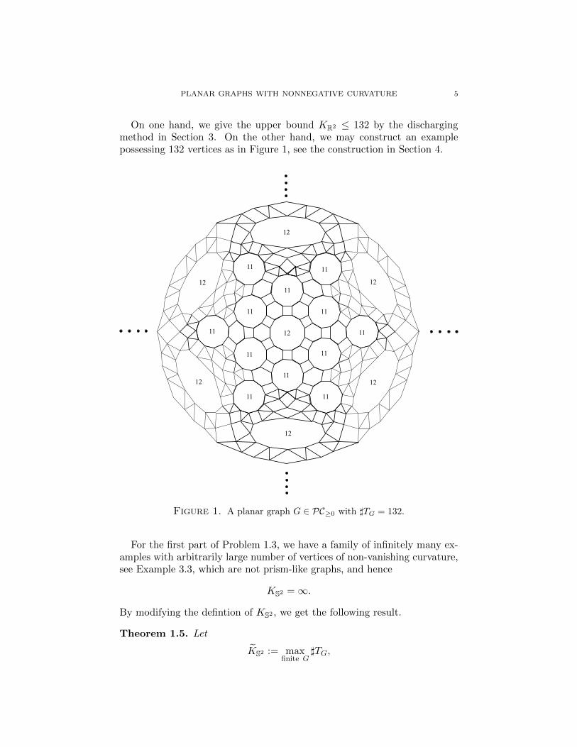
On one hand, we give the upper bound KR2 ≤ 132 by the dischargingmethod in Section 3. On the other hand, we may construct an examplepossessing 132 vertices as in Figure 1, see the construction in Section 4.

12

12

12

12

12

12

12

11

11

11 11

11

11

11

11

1111

11

11

Figure 1. A planar graph G ∈ PC≥0 with ]TG = 132.

For the first part of Problem 1.3, we have a family of infinitely many ex-amples with arbitrarily large number of vertices of non-vanishing curvature,see Example 3.3, which are not prism-like graphs, and hence

KS2 =∞.

By modifying the defintion of KS2 , we get the following result.

Theorem 1.5. Let

KS2 := maxfinite G

]TG,


where the maximum is taken over finite graphs in PC≥0 whose maximalfacial degree is less than 132. Then

KS2 = 264.

Moreover, a graph in this class attains the maximum if and only if its poly-hedral surface contains 24 disjoint hendecagons.

The proof of the theorem follows from the same argument as in Theo-rem 1.4, see Section 3 and Section 4.

As an application, we may estimate the order of automorphism groupsof planar graphs with nonnegative curvature. The automorphism groupsof planar graphs have been extensively studied in the literature, to cite afew [Man71, Bab75, CBGS08, SS98]. Let G = (V,E, F ) be a planar graph.A bijection R : V → V is called a graph automorphism if it preserves thegraph structure of (V,E). A triple (HV , HE , HF ) with bijections on V, Eand F respectively is called a cellular automorphism of G = (V,E, F ) ifthey preserve the incidence structure of the cell complex G. We denote by

Aut(G) the graph automorphism group of the graph (V,E), and by Aut(G)the cellular automorphism group of the planar graph G, see Section 5 fordefinitions. We prove for any graph G ∈ PC≥0 with positive total curvature,the cellular automorphism group is finite, and give the estimate for the orderof the group.

Theorem 1.6. Let G = (V,E, F ) be a planar graph with nonnegative com-binatorial curvature and Φ(G) > 0. Then we have the following:

(1) If G is infinite, then

]Aut(G) ≤{

132!× 5!, for DG ≤ 42,2DG, for DG > 42.

(2) If G is finite, then

]Aut(G) ≤{

264!× 5!, for DG ≤ 42,4DG, for DG > 42.

Note that Whitney [Whi33] proved a well-known theorem that any finite3-connected planar graph, i.e. remaining connected after deleting any twovertices, can be uniquely embedded into S2. This has been generalized toinfinite graphs by Mohar [Moh88] that a locally finite, 3-connected planargraph, whose faces are bounded by cycles of finite size, has a unique embed-ding in the plane, see also [Imr75, Tho82]. These results imply that for any3-connected planar graph G = (V,E, F ) in our setting,

Aut(G) ∼= Aut(G).

Hence all results in Theorem 1.6 apply to the graph automorphism group ifthe graph is 3-connected.

The paper is organized as follows: In next section, we recall some basicfacts on the combinatorial curvature of planar graphs. Section 3 is devoted to


the upper bound estimates for Theorem 1.4 and Theorem 1.5. In Section 4,we construct examples to show the lower bound estimates for Theorem 1.4and Theorem 1.5. The last section contains the proof of Theorem 1.6.

2. Preliminaries

Let G = (V,E, F ) be a planar graph induced by an embedding of a graph(V,E) into S2 or R2. We only consider the appropriate embedding such thatG is a tessellation of S, see the definition in the introduction. Hence G isa finite graph if and only if it embeds into S2, and G is an infinite graph ifand only if it embeds into R2.

We say that a vertex x is incident to an edge e, denoted by x ≺ e,(similarly, an edge e is incident to a face σ, denoted by e ≺ σ; or a vertexx is incident to a face σ, denoted by x ≺ σ) if the former is a subset of theclosure of the latter. For any face σ, we denote by

∂σ := {x ∈ V : x ≺ σ}the vertex boundary of σ. Two vertices are called neighbors if there is anedge connecting them. We denote by deg(x) the degree of a vertex x, i.e.the number of neighbors of a vertex x, and by deg(σ) the degree of a faceσ, i.e. the number of edges incident to a face σ (equivalently, the number ofvertices incident to σ). Two faces σ and τ are called adjacent, denoted byσ ∼ τ, if there is an edge incident to both of them, i.e. they share a commonedge.

For a planar graph G = (V,E, F ), let S(G) denote the polyhedral surfacewith piecewise flat metric defined in the introduction. For S(G), it is locallyisometric to a flat domain in R2 near any interior point of an edge or aface, while it might be non-smooth near some vertices. As a metric surface,the generalized Gaussian curvature K of S(G) vanishes at smooth pointsand can be regarded as a measure concentrated on the isolated singularities,i.e. on vertices. One can show that the mass of the generalized Gaussiancurvature at each vertex x is given by K(x) = 2π−Σx, where Σx denotes thetotal angle at x in the metric space S(G), see [Ale05]. Moreover, by directcomputation one has K(x) = 2πΦ(x), where the combinatorial curvatureΦ(x) is defined in (2). Hence one can show that a planar graph G hasnonnegative combinatorial curvature if and only if the polyhedral surfaceS(G) is a generalized convex surface.

In a planar graph, the pattern of a vertex x is defined as a vector

(deg(σ1), deg(σ2), · · · , deg(σN )),

whereN = deg(x), {σi}Ni=1 are the faces which x is incident to, and deg(σ1) ≤deg(σ2) ≤ · · · ≤ deg(σN ).

Table 1 is the list of all possible patterns of a vertex with positive cur-vature (see [DM07, CC08]); Table 2 is the list of all possible patterns of avertex with vanishing curvature (see [GS89, CC08]).


Patterns Φ(x)(3, 3, k) 3 ≤ k 1/6 + 1/k(3, 4, k) 4 ≤ k 1/12 + 1/k(3, 5, k) 5 ≤ k 1/30 + 1/k(3, 6, k) 6 ≤ k 1/k(3, 7, k) 7 ≤ k ≤ 41 1/k − 1/42(3, 8, k) 8 ≤ k ≤ 23 1/k − 1/24(3, 9, k) 9 ≤ k ≤ 17 1/k − 1/18(3, 10, k) 10 ≤ k ≤ 14 1/k − 1/15(3, 11, k) 11 ≤ k ≤ 13 1/k − 5/66(4, 4, k) 4 ≤ k 1/k(4, 5, k) 5 ≤ k ≤ 19 1/k − 1/20(4, 6, k) 6 ≤ k ≤ 11 1/k − 1/12(4, 7, k) 7 ≤ k ≤ 9 1/k − 3/28(5, 5, k) 5 ≤ k ≤ 9 1/k − 1/10(5, 6, k) 6 ≤ k ≤ 7 1/k − 2/15(3, 3, 3, k) 3 ≤ k 1/k(3, 3, 4, k) 4 ≤ k ≤ 11 1/k − 1/12(3, 3, 5, k) 5 ≤ k ≤ 7 1/k − 2/15(3, 4, 4, k) 4 ≤ k ≤ 5 1/k − 1/6(3, 3, 3, 3, k) 3 ≤ k ≤ 5 1/k − 1/6

Table 1. The patterns of a vertex with positive curvature.

(3, 7, 42), (3, 8, 24), (3, 9, 18), (3, 10, 15), (3, 12, 12),(4, 5, 20), (4, 6, 12), (4, 8, 8), (5, 5, 10), (6, 6, 6),(3, 3, 4, 12), (3, 3, 6, 6), (3, 4, 4, 6), (4, 4, 4, 4), (3, 3, 3, 3, 6),(3, 3, 3, 4, 4), (3, 3, 3, 3, 3, 3).

Table 2. The patterns of a vertex with vanishing curvature.

The following lemma is useful for our purposes, see [CC08, Lemma 2.5].

Lemma 2.1. If there is a face σ such that deg(σ) ≥ 43 and Φ(x) ≥ 0 forany vertex x incident to σ, then∑

x∈V :x≺σΦ(x) ≥ 1.

For an infinite planar graph G with nonnegative curvature if there is aface of degree at least 43, then the graph has rather special structure, see[HJL15, Theorem 2.10]. As in the introduction, we call it an infinite prisim-like graph. By dividing hexagons into triangles, one may assume that thereis no hexagon in G.

Theorem 2.2 ([HJL15]). Let G = (V,E, F ) be a planar graph with non-negative curvature and DG ≥ 43. Then there is only one face σ of degree at


least 43. Suppose that there is no hexagonal face. Then the set of faces Fconsists of σ, triangles or squares. Moreover,

S(G) = σ ∪ (∪∞i=1Li),

where Li, i ≥ 1, is a set of faces of the same type (triangle or square) whichcomposite a band, i.e. an annulus, such that

minx∈∪τ∈Li∂τ,

y∈∂σ

d(x, y) = i− 1,

where d is the graph distance in (V,E). And S(G) is isometric to the bound-ary of a half flat-cylinder in R3, see Figure 2.

σ

Figure 2. A half flat-cylinder in R3.

We collect some properties of an infinite prism-like graph:

• There is only one face σ of degree at least 43, and deg(σ) = DG;• TG consists of all vertices incident to the largest face σ;• Any face, which is not σ, is either a triangle, a square or a hexagon;• The polygonal surface S(G) is isometric to the boundary of a half

flat-cylinder in R3.• Φ(G) = 1.

Next, we study finite prism-like graphs. Recall that a finite graph G withnonnegative curvature is called prism-like if the number of faces with degreeat least 43 is at least two.

Theorem 2.3. Let G = (V,E, F ) be a finite prism-like graph. Then thereare exactly two disjoint faces σ1 and σ2 of same facial degree at least 43.Suppose that there is no hexagonal face. Then the set of faces F consists ofσ1 and σ2, triangles or squares. Moreover,

S(G) = σ1 ∪ (∪Mi=1Li) ∪ σ2,

where M ≥ 1, Li, 1 ≤ i ≤M, is a set of faces of the same type (triangle orsquare) which composite a band, i.e. an annulus, such that

minx∈∪τ∈Li∂τ,y∈∂σ1

d(x, y) = i− 1.


And S(G) is isometric to the boundary of a cylinder barrel in R3, see Fig-ure 3.

σ1 σ2

Figure 3. A cylinder barrel in R3.

Proof. We adopt the same argument as in the proof of Theorem 2.2 in[HJL15]. Since the curvature is nonnegative, one is ready to see that theboundaries of any two faces of degree at least 43 are disjoint. By Lemma 2.1,for any face σ of degree at least 43,∑

x∈V :x≺σΦ(x) ≥ 1.

Since the graph is finite, by Gauss-Bonnet theorem, Φ(G) = 2. Hence thereare exactly two faces of degree at least 43, denoted by σ1 and σ2. Moreover,we have ∑

x∈V :x≺σi

Φ(x) = 1, i = 1, 2,

and Φ(x) = 0, for any x ∈ V \(∂σ1∪∂σ2). For any x ∈ ∂σ1∪∂σ2, the patternof x is (4, 4, ki) or (3, 3, 3, ki), where ki = deg(σi) for i = 1, 2. Suppose thatthere is a vertex x ∈ ∂σ1 whose pattern is (4, 4, k1) ((3, 3, 3, k1) resp.), thenthe patterns of all vertices in ∂σ1 are (4, 4, k1) ((3, 3, 3, k1) resp.). Sameresults hold for ∂σ2. We denote by L1 the set of all faces incident to σ1

which composite a band. Inductively, for any i ≥ 1 define Li+1 as the setof faces incident to one of Li, which are not in σ1 ∪ (∪i−1

j=1Lj). Note thatLi, i ≥ 1, consists of faces of same degree, triangles or squares. Since thegraph is finite, there is some M such that σ2 is incident to some face in LM .Considering the properties of faces incident to σ2 similarly, we have all facesin LM are incident to σ2. This yields that deg(σ1) = deg(σ2) and proves thetheorem. �

A finite prism-like graph G has the following properties:

• There are exactly two faces σ1 and σ2 of degree at least 43;• deg(σ1) = deg(σ2);• TG consists of all vertices in ∂σ1 ∪ ∂σ2;• Any face, which is not σ1 and σ2, is either a triangle, a square or a

hexagon;


• The polygonal surface S(G) the boundary of a cylinder barrel in R3.

3. Upper bound estimates for the size of TG

In this section, we prove the upper bound estimates for the number ofvertices in TG for planar graph G with nonnegative curvature.

Definition 3.1. We say that a vertex x ∈ TG is bad if 0 < Φ(x) < 1132 , and

good if Φ(x) ≥ 1132 .

Let G ∈ PC≥0 be either an infinite graph or a finite graph with DG < 132,which is not a prism-like graph. Then direct computation shows that allpatterns of bad vertices of G are given by

(3, 7, k), 32 ≤ k ≤ 41, (3, 8, k), 21 ≤ k ≤ 23, (3, 9, k), 16 ≤ k ≤ 17

(3, 10, 14), (3, 11, 13), (4, 5, k), 18 ≤ k ≤ 19, (4, 7, 9).

Our main tool to prove the results is the discharging method, see e.g.[AH77, RSST97, Moh02, DM07, Oh17, Ghi17]. The curvature at vertices ofa planar graph can be regarded as the charge concentrated on vertices. Thedischarging method is to redistribute the charge on vertices, via transferringthe charge on good vertices to bad vertices, such that the final/terminalcharge on involved vertices is uniformly bounded below. In the following,we don’t distinguish the charge with the curvature. We need to show thatfor each bad vertex in TG, one can find some nearby vertices with a fairamount of curvature, from which the bad vertex will receive some amount ofcurvature. By the discharging process, we get the final curvature uniformlybounded below on TG by the constant 1

132 , so that it yields the upper boundof the cardinality of TG by the upper bound of total curvature. Generallyspeaking, since the discharging method is divided into several steps, one shallcheck that there remains enough amount of curvature at the vertices whichare involved in two or more steps to contribute the curvature. However,in our discharging method, we distribute the curvature at each vertex onlyonce.

Proof of Theorem 1.4 (Upper bound). In the following, we prove the upperbound estimate

KR2 ≤ 132.

Let G ∈ PC≥0 be an infinite graph which is not a prism-like graph. We willintroduce a discharging process to distribute some amount of the curvatureat good vertices to bad vertices via the discharging rules. We denoted by Φ

the curvature at vertices of G and by Φ the final curvature at vertices aftercarrying out the following discharging rules. We will show that the final

curvature satisfies∑

x∈V Φ(x) =∑

x∈V Φ(x), and

Φ(x) ≥ 1

132, ∀x ∈ TG.

This will imply the upper bound estimate ]TG ≤ 132 since the total curva-ture Φ(G) ≤ 1.


The proof consists of three steps: In the first step, we consider the casesfor bad vertices, (3, 8, k), 21 ≤ k ≤ 23, (3, 9, k), 16 ≤ k ≤ 17, (3, 10, 14) and(3, 11, 13); In the second step, we deal with the cases, (3, 7, k), 32 ≤ k ≤ 41and (4, 7, 9); The last step is devoted to the cases, (4, 5, k), 18 ≤ k ≤ 19.

Step 1. In this step, we divide it into the following three cases:

Case 1.1: There is at least one bad vertex on some k-gon with 21 ≤k ≤ 23. In this case, the pattern of bad vertices must be (3, 8, k). Fixa bad vertex a of the k-gon, see Figure 4. Then we will show that thevertices x, y of the octagon in Figure 4 and the good vertices on thek-gon have enough curvature to be distributed to all bad vertices of

k-gon such that the final curvature Φ at vertices involved is greaterthan 1

132 . In fact, all the possible patterns of x and y are

(4) (3,m, 8), 3 ≤ m ≤ 8, (3, 3, 3, 8) and (3, 3, 4, 8).

a

x y

x' y'

A

8

k

Figure 4. The case for bad vertices of the pattern (3, 8, k) for21 ≤ k ≤ 23.

Note that the curvature of vertices on the k-gon is at least 1k −

124 ,

and for 21 ≤ k ≤ 23,

(5) 2× 13

176+ k

(1

k− 1

24

)≥ k + 2

132.

By the above equation (5), if we can find the sets of good verticeson the k-gon, Ax and Ay, satisfying that• Ax ∩Ay = ∅,• Φ(x) +

∑z∈Ax

Φ(z)− ]Ax ·(

1k −

124

)> 13

176 and

• Φ(y) +∑z∈Ay

Φ(z)− ]Ay ·(

1k −

124

)> 13

176 ,

then x, y, Ax and Ay have enough curvature to be distributed to allbad vertices of the k-gon. In the following, we try to find the setsAx and Ay case by case.


x

z

8

k

(a)

x

z

8

k

(b)

x

z

8

k

(c)

Figure 5. Three situations in Subcase 1.1.2.

Note that all possible patterns listed in (4) except (3, 3, 4, 8) havecurvature at least 1

12 which is strictly greater than 13176 . First, we

consider the pattern of the vertex x. It splits into the following twosubcases:

Subcase 1.1.1: x is not of the pattern (3, 3, 4, 8). We take Ax =∅.

Subcase 1.1.2: x is of the pattern (3, 3, 4, 8). In this situation,we have three cases, as depicted in Figure 5. In either case,Φ(z) ≥ 1

k , i.e. z has a fair amount of curvature, and

Φ(x) + Φ(z)−(

1

k− 1

24

)≥ 1

12>

13

176.

We take Ax = {z}.Considering the pattern of the vertex y, we may choose the set

Ay similarly as Ax above. It is easy to check that Ax and Ay satisfythe conditions as required. This finishes the proof for this case.

Remark 3.2. Note that the only edge of the octagon which could beincident to another l-gon with 21 ≤ l ≤ 23 is the edge A, see Figure4. Hence we can distribute the curvature of vertices x′ and y′ to badvertices on the l-gon. This means that the curvature at every vertexon the octagon is transferred to other bad vertices in the dischargingprocess no more than once.

Case 1.2: There is at least one bad vertex on some k-gon with 16 ≤k ≤ 17. In this case, the pattern of bad vertices must be (3, 9, k).The situation is similar to Case 1.1. We can argue verbatim as aboveto conclude the results, and hence omit the proof here.

Case 1.3: There is at least one bad vertex on some 14-gon. In thiscase, the pattern of bad vertices must be (3, 10, 14). We can use asimilar argument as in Case 1.1 and omit the proof here.

Case 1.4: There is at least one bad vertex on some tridecagon, de-noted by σ. In this case, the pattern of bad vertices must be


(3, 11, 13), see Figure 6. Note that all possible patterns of x andy are

(3,m, 11), 3 ≤ m ≤ 11, (3, 3, 3, 11) and (3, 3, 4, 11).

13, σ

11x

ya

Figure 6. The case for bad vertices of the pattern (3, 11, 13).

Note that the curvature of vertices on the tridecagon σ is at least1

858 and the following holds,

2× 13

264+ 13× 1

858=

13 + 2

132.

Suppose that we can find the sets of good vertices, Ax, Ay, Bx andBy, satisfying that• (Ax ∪Ay) ⊂ ∂σ, (Bx ∪By) ∩ (∂σ ∪ {x, y}) = ∅,• (Ax ∪Bx) ∩ (Ay ∪By) = ∅,• Φ(x) +

∑z∈Ax

Φ(z)− ]Ax858 +

∑z∈Bx

Φ(z)− ]Bx132 >

13264 and

• Φ(y) +∑z∈Ay

Φ(z)− ]Ay858 +

∑z∈By

Φ(z)− ]By132 >

13264 .

Then x, y, Ax, Ay, Bx and By have enough curvature to be dis-tributed to all bad vertices of the tridecagon.

For our purposes, we first consider the case that the pattern of xis not of the pattern (3, 11, 11). Then we have the following cases,A–D.

A: The pattern of x is one of (3, 3, 11), (3, 4, 11), (3, 5, 11), (3, 6, 11),(3, 7, 11) and (3, 3, 3, 11). In this subcase, since Φ(x) > 13

264 , wetake Ax = ∅ and Bx = ∅.

B: x is of the pattern (3, 8, 11) or (3, 9, 11), see Figure 7. In thissubcase, noting that Φ(x) + Φ(z) − 1

858 > 13264 , we can take

Ax = {z} and Bx = ∅.


13

x

y

118,9

az

Figure 7. The case that the pattern of x is (3, 8, 11) or (3, 9, 11).

C: x is of the pattern (3, 10, 11), see Figure 8. In this subcase,noting that Φ(w′) ≥ 1

60 , we have

Φ(x) + Φ(z) + Φ(w) +

(Φ(w′)− 1

132

)− 2

858>

13

264.

We can take Ax = {z, w} and Bx = {w′}. Note that in thissituation, the curvature at the vertex w′ is not distributed tothe vertices of some 14-gon or other tridecagon, since the edgeA cannot be incident to any 14-gon or tridecagon. That is, weonly distribute the curvature of w′ to other vertices once.

13

1110x

yzww'

a

A

Figure 8. The case that the pattern of x is (3, 10, 11).

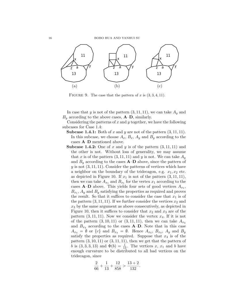
D: x is of the pattern (3, 3, 4, 11). There are three possible sit-uations, as depicted in Figure 9. In either case, Φ(z) ≥ 1

13 ,hence

Φ(x) + Φ(z)−(

1

13− 5

66

)≥ 13

264.

We take Ax = {z} and Bx = ∅.


13

11x

yz a

(a)

13

11x

yaz

(b)

13

11x

yz a

(c)

Figure 9. The case that the pattern of x is (3, 3, 4, 11).

In case that y is not of the pattern (3, 11, 11), we can take Ay andBy according to the above cases, A–D, similarly.

Considering the patterns of x and y together, we have the followingsubcases for Case 1.4:

Subcase 1.4.1: Both of x and y are not of the pattern (3, 11, 11).In this subcase, we choose Ax, Bx, Ay and By according to thecases A–D mentioned above.

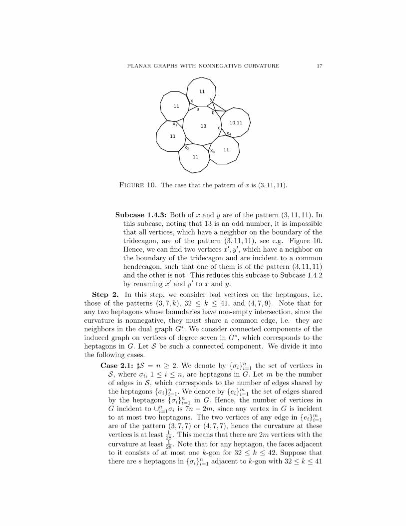
Subcase 1.4.2: One of x and y is of the pattern (3, 11, 11) andthe other is not. Without loss of generality, we may assumethat x is of the pattern (3, 11, 11) and y is not. We can take Ayand By according to the cases A–D above, since the pattern ofy is not (3, 11, 11). Consider the patterns of vertices which havea neighbor on the boundary of the tridecagon, e.g. x1, x2 etc.as depicted in Figure 10. If x1 is not of the pattern (3, 11, 11),then we can take Ax1 and Bx1 for the vertex x1 according to thecases A–D above. This yields four sets of good vertices Ax1 ,Bx1 , Ay and By satisfying the properties as required and provesthe result. So that it suffices to consider the case that x1 is ofthe pattern (3, 11, 11). If we further consider the vertices x2 andx3 by the same argument as above consecutively, as depicted inFigure 10, then it suffices to consider that x2 and x3 are of thepattern (3, 11, 11). Now we consider the vertex x4. If it is notof the pattern (3, 10, 11) or (3, 11, 11), then we can take Ax4and Bx4 according to the cases A–D. Note that in this caseAx4 = ∅ or {c} and Bx4 = ∅. Hence Ax4 , Bx4 , Ay and Bysatisfy the properties as required. Suppose that x4 is of thepattern (3, 10, 11) or (3, 11, 11), then we get that the pattern ofb is (3, 3, 3, 13) and Φ(b) = 1

13 . The vertices x, x1 and b haveenough curvature to be distributed to all bad vertices on thetridecagon, since

2

66+

1

13+

12

858>

13 + 2

132.


13

11

11

11

11

11

10,11

yx

x1

x2 x3

x4

ab

c

Figure 10. The case that the pattern of x is (3, 11, 11).

Subcase 1.4.3: Both of x and y are of the pattern (3, 11, 11). Inthis subcase, noting that 13 is an odd number, it is impossiblethat all vertices, which have a neighbor on the boundary of thetridecagon, are of the pattern (3, 11, 11), see e.g. Figure 10.Hence, we can find two vertices x′, y′, which have a neighbor onthe boundary of the tridecagon and are incident to a commonhendecagon, such that one of them is of the pattern (3, 11, 11)and the other is not. This reduces this subcase to Subcase 1.4.2by renaming x′ and y′ to x and y.

Step 2. In this step, we consider bad vertices on the heptagons, i.e.those of the patterns (3, 7, k), 32 ≤ k ≤ 41, and (4, 7, 9). Note that forany two heptagons whose boundaries have non-empty intersection, since thecurvature is nonnegative, they must share a common edge, i.e. they areneighbors in the dual graph G∗. We consider connected components of theinduced graph on vertices of degree seven in G∗, which corresponds to theheptagons in G. Let S be such a connected component. We divide it intothe following cases.

Case 2.1: ]S = n ≥ 2. We denote by {σi}ni=1 the set of vertices inS, where σi, 1 ≤ i ≤ n, are heptagons in G. Let m be the numberof edges in S, which corresponds to the number of edges shared bythe heptagons {σi}ni=1. We denote by {ei}mi=1 the set of edges sharedby the heptagons {σi}ni=1 in G. Hence, the number of vertices inG incident to ∪ni=1σi is 7n − 2m, since any vertex in G is incidentto at most two heptagons. The two vertices of any edge in {ei}mi=1are of the pattern (3, 7, 7) or (4, 7, 7), hence the curvature at thesevertices is at least 1

28 . This means that there are 2m vertices with the

curvature at least 128 . Note that for any heptagon, the faces adjacent

to it consists of at most one k-gon for 32 ≤ k ≤ 42. Suppose thatthere are s heptagons in {σi}ni=1 adjacent to k-gon with 32 ≤ k ≤ 41


x yz

k

77

w

u

(a)

7

9

k

x

y z

(b)

x

k

7

9

y z

(c)

Figure 11. The heptagon is adjacent to a k-gon for 32 ≤ k ≤ 41.

and there are t heptagons in {σi}ni=1 adjacent to 42-gon. Clearlys + t ≤ n. Hence, there are 2s vertices with the curvature at least

11722 and 2t vertices with vanishing curvature. The curvature of other

vertices is at least 1252 . Since m ≥ n− 1 > 46

109n for n ≥ 2, we have

2m

28+

2s

1722+

7n− 2m− 2(s+ t)

252≥ 2m

28+

5n− 2m

252>

7n− 2m

132.

This means that good vertices on these heptagons have enough cur-vature to be distributed to bad vertices on them.

Case 2.2: ]S = 1. For the heptagon in S, the intersection of its bound-ary and the boundary of any other heptagon in G is empty. Weconsider this isolated heptagon and divide it into the following threesubcases:

Subcase 2.2.1: The heptagon is adjacent to a k-gon for 32 ≤k ≤ 41, and there is no vertices on the heptagon of the pattern(4, 7, 9), see Figure 11(a). In this subcase, all possible patternsof the vertices on k-gon are (3, 3, k), (3, 4, k), (3, 5, k), (3, 6, k),(3, 7, k), (4, 4, k) and (3, 3, 3, k). Except the pattern (3, 7, k), allpatterns have the curvature at least 1

k . Note that the patternof z cannot be (3, 7, k). Otherwise, the vertex u, as depicted inFigure 11(a), would be of pattern (3, 7, 7) which will imply thattwo heptagons are adjacent to each other and yields a contradic-tion to the assumption. Hence Φ(z) ≥ 1

k . Denote by w the firstvertex on the boundary of the k-gon in the direction from y to xwhich is of the pattern (3, 7, k). If the heptagon which containsw belongs to Case 2.1, i.e. it is incident to another heptagon,then we distribute the curvature at z only to x. Otherwise, wedistribute the curvature at z to both x and w. For the vertexy, we can use a similar argument to derive the result.

Subcase 2.2.2: The heptagon is adjacent to a k-gon for 32 ≤ k ≤41, and there exists at least one vertex on the heptagon of thepattern (4, 7, 9). In this subcase, there are two situations, see


Figure 11(b, c). In either case, note that the pattern of x mustbe (3, 3, 4, 7) and Φ(x) = 5

84 , which is enough to be distributedto bad vertices of the pattern (4, 7, 9), since there are at mosttwo such bad vertices on the heptagon. And bad vertices of thepattern (3, 7, k), i.e. the vertices y, z in Figure 11 (b, c), can betreated in the same way as in Subcase 2.2.1.

Subcase 2.2.3: The heptagon is not adjacent to any k-gon for32 ≤ k ≤ 41. That is, all bad vertices are of the pattern (4, 7, 9).Fix a vertex x on the heptagon of the pattern (4, 7, 9), see Figure12. For the vertex y, we have the following possible situations:

Subcase 2.2.3(A): If the pattern of y is (3, 7, 9) and z isnot of the pattern (3, 7, l) for 16 ≤ l ≤ 17, then the curva-ture at y has not been distributed to other vertices before.And by the fact that Φ(y) = 11

126 > 7132 , y has enough

curvature to be distributed to all bad vertices on the hep-tagon.If the pattern of y is (3, 7, 9) and z is of the pattern(3, 7, l) for 16 ≤ l ≤ 17, see Figure 12(a), then the cur-vature at y might have been distributed to bad verticesof the l-gon in Step 1. However, since z and w, as de-picted in Figure 12(a), must be of the pattern (3, 7, l) andmin{Φ(z),Φ(w)} ≥ 25

714 , they have enough curvature tobe distributed to all bad vertices of the heptagon.

Subcase 2.2.3(B): If the pattern of y is (4, 7, 9), then weconsider the vertex z, see Figure 12(b). By the assump-tion, z cannot be of pattern (4, 7, 7). If z is not of thepattern (4, 7, 8) or (4, 7, 9), then Φ(z) ≥ 5

84 >7

132 , hencez has enough curvature to be distributed to bad verticeson the heptagon. If the pattern of z is (4, 7, 8) ((4, 7, 9)resp.) and the pattern of w is (3, 7, 8) ((3, 7, 9) resp.),we can get the conclusion by a similar argument as inthe situation Subcase 2.2.3(A) above where y is of thepattern (3, 7, 9). If the pattern of w is (4, 7, 8), which im-plies that the pattern of z must be (4, 7, 8), then we haveΦ(z) + Φ(w) = 1

28 . They have enough curvature to bedistributed to bad vertices of the heptagon, since

1

28+

5

252>

7

132.

If the pattern of w is (4, 7, 9), then the pattern of z mustbe (4, 7, 9). Similarly, we consider s and t, if s or t isnot (4, 7, 9), the conclusion is obvious. If all of them are(4, 7, 9), then u is of the pattern (4, 4, 7) which has enoughcurvature to distribute.


7

9

yx

z

w

l

(a)

9

7

x y

z

ws

t

u

(b)

Figure 12. The heptagon is not adjacent to any k-gon for 32 ≤k ≤ 41.

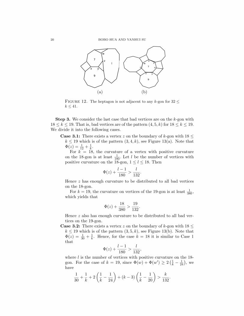
Step 3. We consider the last case that bad vertices are on the k-gon with18 ≤ k ≤ 19. That is, bad vertices are of the pattern (4, 5, k) for 18 ≤ k ≤ 19.We divide it into the following cases.

Case 3.1: There exists a vertex z on the boundary of k-gon with 18 ≤k ≤ 19 which is of the pattern (3, 4, k), see Figure 13(a). Note thatΦ(z) = 1

12 + 1k .

For k = 18, the curvature of a vertex with positive curvatureon the 18-gon is at least 1

180 . Let l be the number of vertices withpositive curvature on the 18-gon, 1 ≤ l ≤ 18. Then

Φ(z) +l − 1

180>

l

132.

Hence z has enough curvature to be distributed to all bad verticeson the 18-gon.

For k = 19, the curvature on vertices of the 19-gon is at least 1380 ,

which yields that

Φ(z) +18

380>

19

132.

Hence z also has enough curvature to be distributed to all bad ver-tices on the 19-gon.

Case 3.2: There exists a vertex z on the boundary of k-gon with 18 ≤k ≤ 19 which is of the pattern (3, 5, k), see Figure 13(b). Note thatΦ(z) = 1

30 + 1k . Hence, for the case k = 18 it is similar to Case 1

that

Φ(z) +l − 1

180>

l

132,

where l is the number of vertices with positive curvature on the 18-gon. For the case of k = 19, since Φ(w) + Φ(w′) ≥ 2

(1k −

124

), we

have

1

30+

1

k+ 2

(1

k− 1

24

)+ (k − 3)

(1

k− 1

20

)>

k

132.


18,19z

(a)

18,19a w

w'

(b)

18,19ax y

(c)

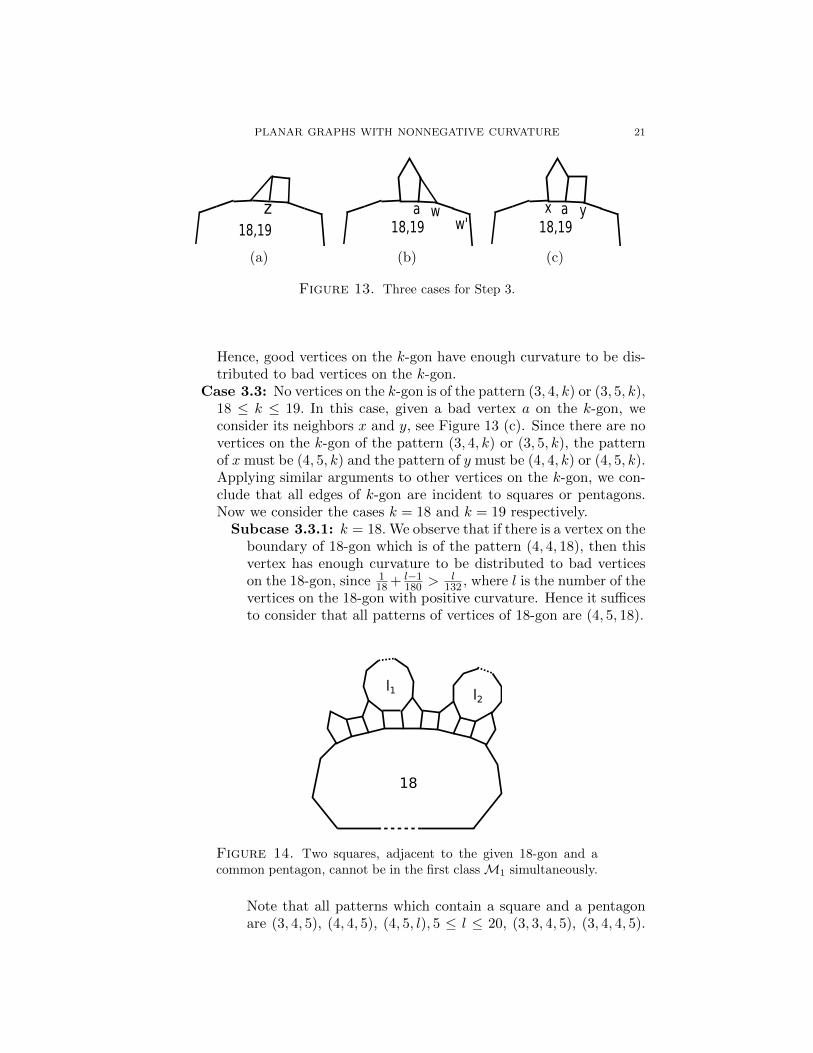
Figure 13. Three cases for Step 3.

Hence, good vertices on the k-gon have enough curvature to be dis-tributed to bad vertices on the k-gon.

Case 3.3: No vertices on the k-gon is of the pattern (3, 4, k) or (3, 5, k),18 ≤ k ≤ 19. In this case, given a bad vertex a on the k-gon, weconsider its neighbors x and y, see Figure 13 (c). Since there are novertices on the k-gon of the pattern (3, 4, k) or (3, 5, k), the patternof x must be (4, 5, k) and the pattern of y must be (4, 4, k) or (4, 5, k).Applying similar arguments to other vertices on the k-gon, we con-clude that all edges of k-gon are incident to squares or pentagons.Now we consider the cases k = 18 and k = 19 respectively.

Subcase 3.3.1: k = 18.We observe that if there is a vertex on theboundary of 18-gon which is of the pattern (4, 4, 18), then thisvertex has enough curvature to be distributed to bad verticeson the 18-gon, since 1

18 + l−1180 >

l132 , where l is the number of the

vertices on the 18-gon with positive curvature. Hence it sufficesto consider that all patterns of vertices of 18-gon are (4, 5, 18).

18

l1 l2

Figure 14. Two squares, adjacent to the given 18-gon and acommon pentagon, cannot be in the first classM1 simultaneously.

Note that all patterns which contain a square and a pentagonare (3, 4, 5), (4, 4, 5), (4, 5, l), 5 ≤ l ≤ 20, (3, 3, 4, 5), (3, 4, 4, 5).


18,19

a b c d

(a)

19

a b c d

(b)

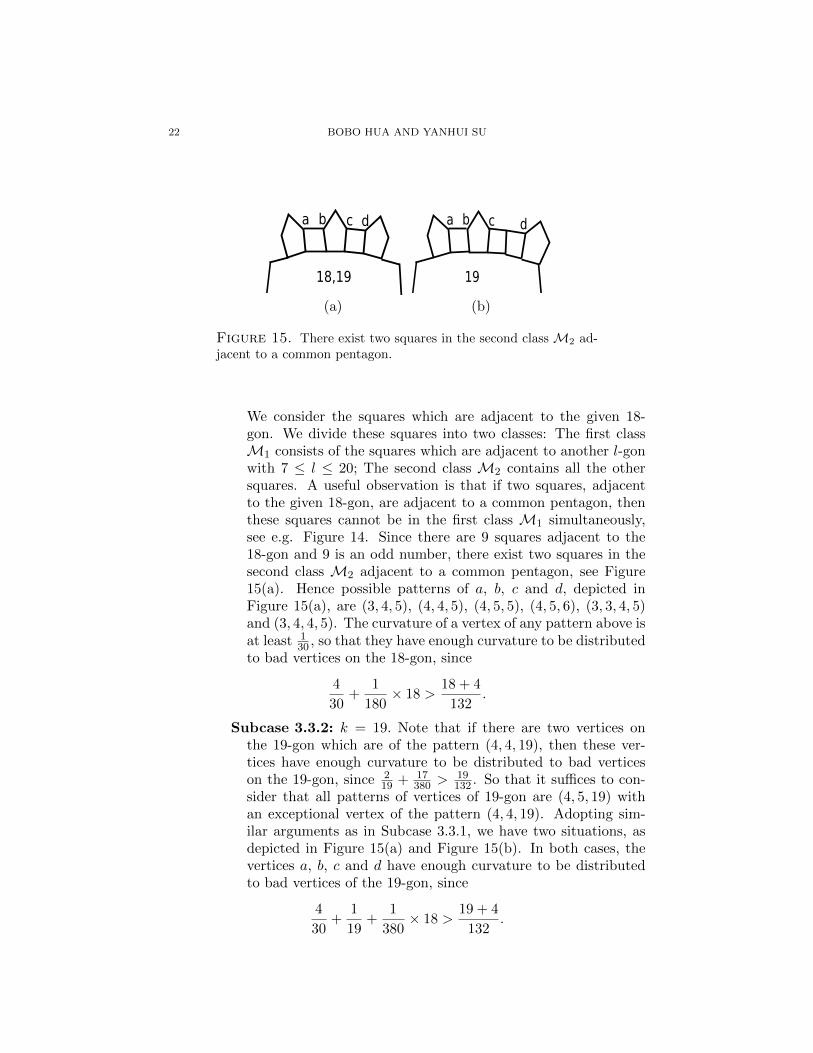
Figure 15. There exist two squares in the second class M2 ad-jacent to a common pentagon.

We consider the squares which are adjacent to the given 18-gon. We divide these squares into two classes: The first classM1 consists of the squares which are adjacent to another l-gonwith 7 ≤ l ≤ 20; The second class M2 contains all the othersquares. A useful observation is that if two squares, adjacentto the given 18-gon, are adjacent to a common pentagon, thenthese squares cannot be in the first class M1 simultaneously,see e.g. Figure 14. Since there are 9 squares adjacent to the18-gon and 9 is an odd number, there exist two squares in thesecond class M2 adjacent to a common pentagon, see Figure15(a). Hence possible patterns of a, b, c and d, depicted inFigure 15(a), are (3, 4, 5), (4, 4, 5), (4, 5, 5), (4, 5, 6), (3, 3, 4, 5)and (3, 4, 4, 5). The curvature of a vertex of any pattern above isat least 1

30 , so that they have enough curvature to be distributedto bad vertices on the 18-gon, since

4

30+

1

180× 18 >

18 + 4

132.

Subcase 3.3.2: k = 19. Note that if there are two vertices onthe 19-gon which are of the pattern (4, 4, 19), then these ver-tices have enough curvature to be distributed to bad verticeson the 19-gon, since 2

19 + 17380 >

19132 . So that it suffices to con-

sider that all patterns of vertices of 19-gon are (4, 5, 19) withan exceptional vertex of the pattern (4, 4, 19). Adopting sim-ilar arguments as in Subcase 3.3.1, we have two situations, asdepicted in Figure 15(a) and Figure 15(b). In both cases, thevertices a, b, c and d have enough curvature to be distributedto bad vertices of the 19-gon, since

4

30+

1

19+

1

380× 18 >

19 + 4

132.


Combining all cases above, we distribute the curvature at good vertices

to bad vertices such that all vertices in TG has final curvature Φ uniformlybounded below by 1

132 . This proves the upper bound ]TG ≤ 132. For theequality case, suppose that G has ]TG = 132, since all the inequalities inthe discharge method is strictly, then there are no bad vertices in TG andall of them have curvature 1

132 . The vertex pattern of curvature 1132 is given

by (3, 3, 4, 11), (4, 6, 11), or (3, 11, 12). Hence, G has exactly 12 disjoint hen-decagons. �

Now we study finite planar graphs with nonnegative curvature. First atall, we show that there are infinitely many finite planar graphs with a largeface which are not prism-like graphs. This indicates that the upper boundof maximal facial degree 132 in Theorem 1.5 is somehow necessary.

Example 3.3. For any even number m ≥ 8, there is a finite planar graphGm ∈ PC≥0, which is not a prism-like graph, such that it has a unique faceof degree m and all the other faces are triangles and squares. Moreover,

]TG = m+ 4

which yields that KS2 =∞, see Problem 1.3 for the definition.

Figure 16. A finite graph has many vertices with positive cur-vature, which is not prism-like.

Proof. Write m = 2(a+b+2) for some a ≥ 1, b ≥ 1. We construct a rectangleof side length a and b, consisting of a×b squares, and attach 2(a+b) squaresalong the sides of the rectangle and 4 triangles to four corners. We obtain aconvex domain as in Figure 16 whose boundary consisting of m edges. Nowglue an m-gon along the boundary of the domain, we get a planar graph asdesired. �

Proof of Theorem 1.5 (Upper bound). LetG be a finite planar graph in PC≥0

with DG < 132, which is not a prism-like graph. Note that our dischargingmethod in the proof of Theorem 1.4 is local, one can distribute the curvature

to bad vertices such that the modified curvature Φ ≥ 1132 on TG. Then by

Φ(G) = 2, one gets the upper bound 264. For the equality case, one canargue similarly as in the proof of Theorem 1.4. �


4. Constructions of large planar graphs with nonnegativecurvature

In this section, we prove the lower bound estimates for the number of ver-tices in TG for a planar graph G with nonnegative curvature in Theorem 1.4and Theorem 1.5 by constructing examples.

In the first part of the section, we consider infinite planar graphs. Asshown in the introduction, there is an infinite planar graph G ∈ PC≥0 whichis not a prism-like graph with ]TG = 132, see Figure 1. By this example, wegive the lower bound estimate of KR2 ≥ 132 in Theorem 1.4. However, in arigorous manner we need to show that the graph in Figure 1 can be furtherextended up to infinity, so as to guarantee that it is a planar tessellation.

We cut off a central part of Figure 1 and denote it by PA, shown inFigure 17. Then the annular part surrounding it in Figure 1 is denoted byPB, shown in Figure 18, in which we have modified the sizes of faces toobtain a nice-looking annular domain.

a3

a1a2

a5

a4

a9

a6a8a7

a11

a10

a12

12

11

11

11

11

11

11

11

11

11

11

11

11

Figure 17. A central part in Figure 1, denoted by PA.

We make infinitely many copies of PB, denoted by {PBi}∞i=1, and gluethese pieces together with PA as follows, see Figure 19:

PA ↔ PB1 ↔ PB2 ↔ PB3 ↔ · · · ↔ PBi ↔ · · · · · · ,

where we denote by G1 ↔ G2 the gluing of two graphs G1 and G2 along theboundaries following the rules:


a1a2

a3

a6

a5

a4

a7

a9

a8

a11

a10

a12

12

12

12

12

1212

b9

b8

b7

b6

b5

b4

b3

b1

b2

b11

b10

b12

Figure 18. An annular part in Figure 1, denoted by PB .

PA PB1 PB2 PB3

Figure 19. The gluing process for the construction of Figure 1.


(1) For G1 = PA and G2 = PB1 , we glue the red boundary in PA withthe red boundary of PB1 by identifying the vertices {ai}12

i=1 in bothgraphs.

(2) For G1 = PBi and G2 = PBi+1 with i ≥ 1, we glue the blue boundaryin PBi with the red boundary of PBi+1 by identifying the vertices

{bi}12i=1 in PBi with the vertices {ai}12

i=1 in PBi+1 .

This constructs the example in Figure 1. One is ready to see that there isa periodic structure for this construction, so that it extends to an infiniteplanar graph embedded into R2.

For the second part of the section, we consider finite planar graphs. Wewill construct a finite planar graph G ∈ PC≥0 with ]TG = 264, which isnot a prism-like graph and has DG = 12. This will give the lower bound

estimate of KS2 ≥ 264 in Theorem 1.5. We make two copies of PA and PBrespectively, denote by PA1 , PA2 , PB1 and PB2 . We glue them together alongthe boundaries as follows

PA1 ↔ PB1 ↔ PB2 ↔ PA2 ,

where PA1 is glued with PB1 along the red boundaries, the blue boundaryof PB1 is glued with the red boundary of PB2 by identifying the vertices{bi}12

i=1 in the former with the vertices {ai}12i=1 in the latter, and the blue

boundary of PB2 is glued with the red boundary of PA2 by identifying thevertices {bi}12

i=1 in the former with the vertices {ai}12i=1 in the latter. This

gives us an example of ]TG = 264.

5. Automorphism groups of planar graphs with nonnegativecurvature

In this section, we study automorphism groups of planar graphs withnonnegative curvature.

First, we introduce several definitions of isomorphisms on planar graphs.

Definition 5.1. Let G1 = (V1, E1, F1) and G2 = (V2, E2, F2) be two planargraphs.

(1) G1 and G2 are said to be graph-isomorphic if there is a graph iso-morphism between (V1, E1) and (V2, E2), i.e. R : V1 → V2 such thatfor any v, w ∈ V, v ∼ w if and only if R(v) ∼ R(w).

(2) G1 and G2 are said to be cell-isomorphic if there is a cellular iso-morphism H = (HV , HE , HF ) between (V1, E1, F1) and (V2, E2, F2)in the sense of cell complexes, i.e. three bijections HV : V1 → V2,HE : E1 → E2 and HF : F1 → F2 preserving the incidence rela-tions, that is, for any v ∈ V, e ∈ E, σ ∈ F, v ≺ e if and only ifHV (v) ≺ HE(e) and e ≺ σ if and only if HE(e) ≺ HF (σ);

(3) G1 and G2 are said to be metric-isomorphic if there is an isomet-ric map in the sense of metric spaces L : S(G1) → S(G2), suchthat the restriction map L is cell-isomorphic between (V1, E1, F1)and (V2, E2, F2).


One is ready to see that metric-isomorphic planar graphs are cell-isomorphic,and hence graph-isomorphic. For a planar graph G, a graph (cellular, met-ric resp.) isomorphism between G and G, i.e. setting G1 = G2 = G in theabove definitions, is called a graph (cellular, metric resp.) automorphism of

G. We denote by Aut(G), (Aut(G), L(G) resp.) the group of graph (cel-lular, metric resp.) automorphisms of a planar graph G. By the standardidentification,

L(G) ≤ Aut(G) ≤ Aut(G),

where ≤ indicates that the former can be embedded as a subgroup of thelatter. By our definition of polyhedral surfaces, it is easy to see that

L(G) ∼= Aut(G).

Moreover, by the results in [Whi33, Moh88] for a 3-connected planar graphG, any graph automorphism R of G can be uniquely realized as a cellularautomorphism H such that HV = R, which is called the associated cellularautomorphism of R. This implies that

L(G) ∼= Aut(G) ∼= Aut(G).

For any G ∈ PC≥0, let H = (HV , HE , HF ) be a cellular automorphismof G. Since for any vertex v ∈ V, Φ(v) = Φ(HV (v)), HV : TG → TG. Thisyields a group homomorphism,

(6) ρ : Aut(G)→ STG , H 7→ HV |TGwhere STG is the permutation group on TG and HV |TG is the restriction ofHV to TG. The kernel of the homomorphism ρ, denoted by ker ρ, consists

of H ∈ Aut(G) such that HV |TG is the identity map on TG. By the groupisomorphism theorem,

Aut(G)/ ker ρ ∼= im(ρ) ≤ STG ,

where im(ρ) denotes the image of the map ρ in STG . To show that Aut(G)is a finite group, it suffices to prove that ker ρ is finite.

We need some basic properties of cellular automorphisms of planar graphs.Recall that for σ1, σ2 ∈ F, we denote by σ1 ∼ σ2 if there is an edge e suchthat e ≺ σ1 and e ≺ σ2. By the definition of planar tessellation in theintroduction, the edge e satisfying the above property is unique. For anyface σ ∈ F, we write the vertex boundary of σ as

∂σ = {v1, v2, · · · , vdeg(σ)}

such that vi ∼ vi+1 for any 1 ≤ i ≤ deg(σ) by setting vdeg(σ)+1 = v1. For acellular automorphism H of a planar graph G, we say that H fixes a face σif HV (v) = v,HE(e) = e and HF (σ) = σ for any v ∈ ∂σ, e ≺ σ, e ∈ E. It iseasy to check that H fixes σ if and only if HV (v) = v for any v ∈ ∂σ. Thefollowing lemma is useful.


Lemma 5.2. Let G = (V,E, F ) be a planar graph and H ∈ Aut(G). Supposethat there are a face σ and {v1, v2} ⊂ ∂σ with v1 ∼ v2 satisfying

HF (σ) = σ,HV (v1) = v1, HV (v2) = v2,

then H fixes the face σ, i.e. HV (v) = v for any v ∈ ∂σ. Moreover, H is theidentity map on G.

Proof. For the first assertion, by HF (σ) = σ we have HV (∂σ) = ∂σ. Wewrite ∂σ = {v1, v2, · · · , vdeg(σ)} such that vi ∼ vi+1 for any 1 ≤ i ≤ deg(σ)by setting vdeg(σ)+1 = v1. Noting that HV (v1) = v1 and HV (v2) = v2, we getthat HV (v3) = v3 since the cellular automorphism H preserves the incidencestructure. The result follows from the induction argument on vi for i ≥ 3.

For the second assertion, it suffices to show that H fixes any face σ ∈ F.Since the dual graph of the planar graph G is connected, there is a sequenceof faces {σj}Mj=0 ⊂ F, M ≥ 1, such that

σ = σ0 ∼ σ1 ∼ · · · ∼ σM = σ.

By the above result, H fixes the face σ0 = σ. Let {v, w} = ∂σ0∩∂σ1. Notingthat HF (σ0) = σ0, HV (v) = v and HV (w) = w, we have HF (σ1) = σ1 bythe incidence preserving property of H. Then one applies the first assertionto σ1, and yields that H fixes σ1. Similarly, the induction argument impliesthat H fixes σj for any 0 ≤ j ≤M. Hence H fixes σ which proves the secondassertion.

�

For any v ∈ TG, we denote by N(v) the set of neighbours of v and by SN(v)

the permutation group on N(v). For any H ∈ ker ρ, it is easy to see thatHV : N(v)→ N(v) since HV (v) = v. This induces a group homomorphism

(7) π : ker ρ→ SN(v), H 7→ HV |N(v).

Lemma 5.3. Let G = (V,E, F ) be a planar graph with nonnegative combi-natorial curvature and positive total curvature. For any v ∈ TG, the map π,defined as in (7), is a group monomorphism.

Proof. It suffices to show that the map π is injective. For any H ∈ kerπ,HV (w) = w, for any w ∈ N(v) ∪ {v}. Let w1, w2 ∈ N(v) such that there isa face σ such that {w1, w2, v} ⊂ ∂σ. By the incidence preserving propertyof H, HF (σ) = σ. Then Lemma 5.2 yields that H is the identity on G. Thisimplies that kerπ is trivial and π is injective. �

Now we are ready to estimate the order of the automorphism group of aplanar graph with nonnegative curvature and positive total curvature.

Theorem 5.4. Let G = (V,E, F ) be a planar graph with nonnegativecombinatorial curvature and positive total curvature. Then the automor-

phism group of G is finite. Set Q(G) := ]Aut(G), a := ]TG and b :=maxv∈TG deg(v). We have the following:


(1) If DG ≤ 42,Q(G) | a!b!.

(2) If DG > 42, then

Q(G) divides

{2DG, G is infinite,4DG, G is finite.

Proof. Suppose that DG ≤ 42, then by Lemma 5.2,

](Aut(G)/ker ρ) | a!,

where ρ is defined in (6). By Lemma 5.3,

] ker ρ | b!.This yields the result.

Suppose that DG > 42, then the planar graph G has some special struc-ture. For simplicity, we write m := DG. We divide it into two cases:

Case 1.: G is infinite. In this case, G is a prism-like graph. By The-orem 2.2, there is only one face σ with deg(σ) = m > 42, andTG = ∂σ. For any H ∈ ker ρ, HF (σ) = σ and HV (v) = v for anyv ∈ TG, so that by Lemma 5.2, H is the identity map on G. Thisyields that

Aut(G) ∼= im(ρ) ≤ STG .For any H ∈ Aut(G), ρ(H) ∈ im(ρ) induces a graph isomorphism onthe cycle graph Cm, which is given by the dihedral group Dm. Thatyields that

im(ρ) ≤ Dm and Q(G)|2m.Case 2.: G is finite. We have two subcases.

Subcase 2.1.: Suppose that ]{σ ∈ F : deg(σ) > 42} ≥ 2, then Gis a finite prism-like graph. By Theorem 2.3, there are exactlytwo faces σ1 and σ2, which are disjoint, of same degree m > 42,

and TG = ∂σ1 ∪ ∂σ2. For any H ∈ Aut(G), HF : {σ1, σ2} →{σ1, σ2}, which yields a group homomorphism

ρ : Aut(G)→ S{σ1,σ2}, H 7→ HF |{σ1,σ2},where S{σ1,σ2} is the permutation group on {σ1, σ2}. This im-plies that

(8) ](Aut(G)/ ker ρ) = 1 or 2.

For any H ∈ ker ρ, HF (σi) = σi for i = 1, 2. Hence HV : ∂σ1 →∂σ1. This yields a group homomorphism

η : ker ρ→ S∂σ1 , H 7→ HV |∂σ1 ,where S∂σ1 is the permutation group on ∂σ1. The same argu-ment as in Case 1 implies that ker η is trivial and im(η) ≤ Dm.Hence

] ker ρ |2m.


By combining it with (8) we have

Q(G)|4m.Subcase 2.2.: Suppose that ]{σ ∈ F : deg(σ) > 42} = 1, then

there is only one face σ ∈ F such that deg(σ) = m. The sameargument as in Case 1 yields that

Q(G)|2m.Combining all cases above, we prove the theorem.

�

By combining the estimates of the size of TG in Theorem 1.4 and The-orem 1.5 with the above result, we obtain the estimates for the orders ofcellular automorphism groups.

Proof of Theorem 1.6. For any G ∈ PC≥0 with DG ≤ 42, we obtain that]TG ≤ 132 if G is infinite by Theorem 1.4, and ]TG ≤ 264 if G is finite byTheorem 1.4. Then the theorem follows from Theorem 5.4. �

Acknowledgements. We thank Wenxue Du for many helpful discus-sions on automorphism groups of planar graphs. Y. S. is supported byNSFC, grant no. 11771083 and NSF of Fujian Province through Grants2017J01556, 2016J01013.

References

[AH77] K. Appel and W. Haken. Every planar map is four colorable. I. Discharging.Illinois J. Math., 21(3):429–490, 1977.

[Ale05] A. D. Alexandrov. Convex polyhedra. Springer Monographs in Mathematics.Springer-Verlag, Berlin, 2005. Translated from the 1950 Russian edition byN. S. Dairbekov, S. S. Kutateladze and A. B. Sossinsky, With comments andbibliography by V. A. Zalgaller and appendices by L. A. Shor and Yu. A.Volkov.

[Bab75] L. Babai. Automorphism groups of planar graphs. II. pages 29–84. Colloq.Math. Soc. Janos Bolyai, Vol. 10, 1975.

[BBI01] D. Burago, Yu. Burago, and S. Ivanov. A course in metric geometry, vol-ume 33 of Graduate Studies in Mathematics. American Mathematical Society,Providence, RI, 2001.

[BD97] G. Brinkmann and A. W. M. Dress. A constructive enumeration of fullerenes.J. Algorithms, 23(2):345–358, 1997.

[BE17a] V. Buchstaber and N. Erokhovets. Finite sets of operations sufficient to con-struct any fullerene from C20. Structural Chemistry, 28(1):225–234, 2017.

[BE17b] V. M. Buchstaber and N. Yu. Erokhovets. Constructions of families of three-dimensional polytopes, characteristic patches of fullerenes, and Pogorelov poly-topes. Izv. Ross. Akad. Nauk Ser. Mat., 81(5):15–91, 2017.

[BGM12] G. Brinkmann, J. Goedgebeur, and B. D. McKay. The generation of fullerenes.J. Chem. Inf. Model., 52(11):2910–2918, 2012.

[BP01] O. Baues and N. Peyerimhoff. Curvature and geometry of tessellating planegraphs. Discrete Comput. Geom., 25(1):141–159, 2001.

[BP06] O. Baues and N. Peyerimhoff. Geodesics in non-positively curved plane tessel-lations. Adv. Geom., 6(2):243–263, 2006.


[CBGS08] J. H. Conway, H. Burgiel, and C. Goodman-Strauss. The symmetries of things.A K Peters, Ltd., Wellesley, MA, 2008.

[CC08] B. Chen and G. Chen. Gauss-Bonnet formula, finiteness condition, and char-acterizations of graphs embedded in surfaces. Graphs Combin., 24(3):159–183,2008.

[Che09] B. Chen. The Gauss-Bonnet formula of polytopal manifolds and the charac-terization of embedded graphs with nonnegative curvature. Proc. Amer. Math.Soc., 137(5):1601–1611, 2009.

[DM07] M. DeVos and B. Mohar. An analogue of the Descartes-Euler formula for infi-nite graphs and Higuchi’s conjecture. Trans. Amer. Math. Soc., 359(7):3287–3300, 2007.

[Gal09] B. Galebach. n-Uniform tilings. Available online athttp://probabilitysports.com/tilings.html, 2009.

[Ghi17] L. Ghidelli. On the largest planar graphs with everywhere positive combina-torial curvature. arXiv:1708.08502, 2017.

[Gro87] M. Gromov. Hyperbolic groups. In Essays in group theory, volume 8 of Math.Sci. Res. Inst. Publ., pages 75–263. Springer, New York, 1987.

[GS89] B. Grunbaum and G. C. Shephard. Tilings and patterns. A Series of Books inthe Mathematical Sciences. W. H. Freeman and Company, New York, 1989.

[Hig01] Y. Higuchi. Combinatorial curvature for planar graphs. J. Graph Theory,38(4):220–229, 2001.

[HJL02] O. Haggstrom, J. Jonasson, and R. Lyons. Explicit isoperimetric constants andphase transitions in the random-cluster model. Ann. Probab., 30(1):443–473,2002.

[HJL15] B. Hua, J. Jost, and S. Liu. Geometric analysis aspects of infinite semiplanargraphs with nonnegative curvature. J. Reine Angew. Math., 700:1–36, 2015.

[HL16] B. Hua and Y. Lin. Curvature notions on graphs. Front. Math. China,11(5):1275–1290, 2016.

[HS03] Y. Higuchi and T. Shirai. Isoperimetric constants of (d, f)-regular planargraphs. Interdiscip. Inform. Sci., 9(2):221–228, 2003.

[HS17] B. Hua and Y. Su. Total curvature of planar graphs with nonnegative curva-ture. arXiv:1703.04119, 2017.

[Imr75] W. Imrich. On Whitney’s theorem on the unique embeddability of 3-connectedplanar graphs. pages 303–306. (loose errata), 1975.

[Ish90] M. Ishida. Pseudo-curvature of a graph. In lecture at Workshop on topologicalgraph theory. Yokohama National University, 1990.

[Kel10] M. Keller. The essential spectrum of the Laplacian on rapidly branching tes-sellations. Math. Ann., 346(1):51–66, 2010.

[Kel11] M. Keller. Curvature, geometry and spectral properties of planar graphs. Dis-crete Comput. Geom., 46(3):500–525, 2011.

[KHO+85] H. W. Kroto, J. R. Heath, S. C. O’Brien, R. F. Curl, and R. E. Smalley. C60

: Buckminsterfullerene. Nature, 318:162–163, 1985.[KP11] M. Keller and N. Peyerimhoff. Cheeger constants, growth and spectrum of

locally tessellating planar graphs. Math. Z., 268(3-4):871–886, 2011.[LPZ02] Serge Lawrencenko, Michael D. Plummer, and Xiaoya Zha. Isoperimetric con-

stants of infinite plane graphs. Discrete Comput. Geom., 28(3):313–330, 2002.[Man71] P. Mani. Automorphismen von polyedrischen Graphen. Math. Ann., 192:279–

303, 1971.[Moh88] B. Mohar. Embeddings of infinite graphs. J. Combin. Theory Ser. B, 44(1):29–

43, 1988.[Moh02] B. Mohar. Light structures in infinite planar graphs without the strong isoperi-

metric property. Trans. Amer. Math. Soc., 354(8):3059–3074, 2002.


[Nev70] R. Nevanlinna. Analytic functions. Translated from the second German editionby Phillip Emig. Die Grundlehren der mathematischen Wissenschaften, Band162. Springer-Verlag, New York-Berlin, 1970.

[NS11] R. Nicholson and J. Sneddon. New graphs with thinly spread positive combi-natorial curvature. New Zealand J. Math., 41:39–43, 2011.

[Oh17] B.-G. Oh. On the number of vertices of positively curved planar graphs. Dis-crete Math., 340(6):1300–1310, 2017.

[Old17] P. R. Oldridge. Characterizing the polyhedral graphswith positive combinatorial curvature. thesis, available athttps://dspace.library.uvic.ca/handle/1828/8030, 2017.

[RBK05] T. Reti, E. Bitay, and Z. Kosztolanyi. On the polyhedral graphs with positivecombinatorial curvature. Acta Polytechnica Hungarica, 2(2):19–37, 2005.

[RSST97] N. Robertson, D. Sanders, P. Seymour, and R. Thomas. The four-colour the-orem. J. Combin. Theory Ser. B, 70(1):2–44, 1997.

[SS98] B. Servatius and H. Servatius. Symmetry, automorphisms, and self-duality ofinfinite planar graphs and tilings. In International Scientific Conference onMathematics. Proceedings (Zilina, 1998), pages 83–116. Univ. Zilina, Zilina,1998.

[Sto76] D. A. Stone. A combinatorial analogue of a theorem of Myers. Illinois J. Math.,20(1):12–21, 1976.

[SY04] L. Sun and X. Yu. Positively curved cubic plane graphs are finite. J. GraphTheory, 47(4):241–274, 2004.

[Tho82] C. Thomassen. Duality of infinite graphs. J. Combin. Theory Ser. B, 33(2):137–160, 1982.

[Thu98] W. P. Thurston. Shapes of polyhedra and triangulations of the sphere. In TheEpstein birthday schrift, volume 1 of Geom. Topol. Monogr., pages 511–549.Geom. Topol. Publ., Coventry, 1998.

[Whi33] H. Whitney. 2-Isomorphic Graphs. Amer. J. Math., 55(1-4):245–254, 1933.[Woe98] W. Woess. A note on tilings and strong isoperimetric inequality. Math. Proc.

Camb. Phil. Soc., 124:385–393, 1998.[Z97] A. Zuk. On the norms of the random walks on planar graphs. Ann. Inst.

Fourier (Grenoble), 47(5):1463–1490, 1997.[Zha08] L. Zhang. A result on combinatorial curvature for embedded graphs on a sur-

face. Discrete Math., 308(24):6588–6595, 2008.

E-mail address: [email protected]

Bobo Hua: School of Mathematical Sciences, LMNS, Fudan University,Shanghai 200433, China; Shanghai Center for Mathematical Sciences, FudanUniversity, Shanghai 200433, China

E-mail address: [email protected]

Yanhui Su: College of Mathematics and Computer Science, Fuzhou Univer-sity, Fuzhou 350116, China

the set of vertices with positive curvature - … vertices with positive curvature in a planar graph...

Documents