the sem approach to longitudinal data analysis using the ... · the sem approach to longitudinal...

Paper SAS1745-2015

The SEM Approach to Longitudinal Data AnalysisUsing the CALIS Procedure

Xinming An and Yiu-Fai Yung, SAS Institute Inc.Qing Yang, Duke University

ABSTRACT

Researchers often use longitudinal data analysis to study the development of behaviors or traits. For example, theymight study how an elderly person’s cognitive functioning changes over time or how a therapeutic intervention affectsa certain behavior over a period of time. This paper introduces the structural equation modeling (SEM) approach toanalyzing longitudinal data. It describes various types of latent curve models and demonstrates how you can use theCALIS procedure in SAS/STAT® software to fit these models. Specifically, the paper covers basic latent curve models,such as unconditional and conditional models, as well as more complex models that involve multivariate responsesand latent factors. All illustrations use real data that were collected in a study that looked at maternal stress and therelationship between mothers and their preterm infants. This paper emphasizes the practical aspects of longitudinaldata analysis. In addition to illustrating the program code, it shows how you can interpret the estimation results andrevise the model appropriately. The final section of the paper discusses the advantages and disadvantages of theSEM approach to longitudinal data analysis.

INTRODUCTION

In longitudinal studies, data are collected from subjects at several time points. The main purpose of longitudinalanalysis is to study the trends or trajectories of the variables of interest. For example, after a medical intervention,health measures might be taken every few months to monitor the health status of patients. Will their health improve,decline, or stay the same in the subsequent months or years? Do all the patients show the same health trajectory?What variables might explain the health trajectories after intervention?

You can use many different statistical approaches to analyze this kind of data, including, but not limited to, econometrictime series (for example, see Chatfield 2003), linear mixed models (for example, see Verbeke and Molenberghs2000), and structural equation modeling (SEM; for example, see Bollen 1989). Gao et al. (2006) show how to analyzelongitudinal data by using different SAS® procedures that are based on different statistical approaches. Differentfields have different traditions, and a particular field might favor one of these approaches or methodologies. Thispaper does not compare these approaches. Rather, it simply adopts the SEM approach and shows how the CALISprocedure can handle several types of models for analyzing longitudinal data. It uses examples to show the modelingflexibility of the SEM approach.

Structural equation modeling has been developed mainly in the social and behavioral sciences. Earlier contributionsare found in the sociological and psychological literature. Structural equation modeling represents the complexrelationships of variables as a sequence of linear equations. A prominent feature that distinguishes SEM from themore mainstream linear statistical modeling is the inclusion of latent factors in SEM. The SEM approach to analyzinglongitudinal data that is described in this paper is often referred to as latent (growth) curve modeling; it is thoroughlydiscussed in an excellent book by Bollen and Curran (2006), where you can find an extensive treatment of themethodology and useful references. Preacher et al. (2008) also provide an excellent introduction to the topic.

The CALIS procedure in SAS/STAT software provides general structural equation modeling capabilities that areuseful for analyzing longitudinal data. Lu and Pearson (2013) use the CALIS procedure to demonstrate the fitting ofunconditional and conditional latent curve models. They also provide a SAS macro to compute some incremental fitindices that are based on more reasonable baseline models. The PROC CALIS chapter in the SAS/STAT manualprovides a simple example of fitting a basic latent curve model. Beyond these sources, there seems to be a scarcity ofPROC CALIS examples to demonstrate the related applications. This paper fills this gap by providing data examplesthat analyze basic and complex latent curve models.

The paper is organized as follows. In the next section, five data-analysis examples demonstrate how to use the CALISprocedure to fit different types of longitudinal models, including unconditional, conditional, and multivariate latent curvemodels. The final section discusses some general advantages and disadvantages of the SEM approach to analyzinglongitudinal data.

1

DATA AND EXAMPLES

This section uses a common data set to illustrate various latent curve models. The data were collected in a researchstudy by Holditch-Davis et al. (2014). The main purpose of the study is to look at the effects of maternally administeredinterventions for preterm infants on the psychological distress of the mother and on the mother-child relationship. Theresearchers recruited 240 mothers who gave birth to preterm infants and randomly assigned them to three treatmentconditions: auditory-tactile-visual-vestibular (ATVV) intervention, kangaroo care (KC), and control. Measurementsand responses, such as demographic information and measures of several psychological symptoms (for example,depression, anxiety, stress, and worry), were taken from these mothers at five time points: during hospitalization; atrelease; and at 2, 6, and 12 months of the corrected age of the infants. See Holditch-Davis et al. (2014) for the detailsof the measurements.

This paper does not use all the responses collected by the researchers. For demonstration purposes, it considers onlythe KC and control conditions and their effects on two specific maternal psychological distress variables: anxiety andworry. These variables were measured using a questionnaire in which the mothers rated themselves on four-pointLikert scales for related items. Twenty items were used for measuring anxiety, and seven items were used formeasuring worry.

Example 1: Basic Unconditional Latent Curve Models for Maternal Anxiety

This example applies the so-called unconditional latent curve model to study the anxiety changes over time underthe KC condition. In this example, anxiety is defined as the sum score of the 20 anxiety items. Only 42 mothersparticipated at every time point, and they have all five anxiety sum scores: anxiety_t1, anxiety_t2, anxiety_t3,anxiety_t4, and anxiety_t5; 38 mothers have incomplete records because they were not present for at least one ofthe time points.

In the unconditional latent curve model, each subject (mother) is assumed to have her own intercept (initial anxietylevel at time point 1) and slope (linear change in anxiety level for each unit change of time). In linear mixed modelterminology, these parameters are called random intercepts and random slopes. In the latent curve modeling approach,these random intercepts and slopes are represented by latent variables that have a multivariate-normal distribution inthe population. These latent variables take the role of factors in structural models.

The following statements specify two unconditional latent curve models for anxiety over time for the KC patients(mothers):

proc calis method=fiml outfit=kang_base; /* Intercept-Only Baseline Model */lineqs

anxiety_t1 = 0. * Intercept + F_Intercept + e1,anxiety_t2 = 0. * Intercept + F_Intercept + e2,anxiety_t3 = 0. * Intercept + F_Intercept + e3,anxiety_t4 = 0. * Intercept + F_Intercept + e4,anxiety_t5 = 0. * Intercept + F_Intercept + e5;

variancee1-e5 = 5 * errv;

meanF_Intercept;

run;

proc calis method=fiml basefit=kang_base; /** Fixed-Loadings Model **/lineqs

anxiety_t1 = 0. * Intercept + F_Intercept + 0. * F_Slope + e1,anxiety_t2 = 0. * Intercept + F_Intercept + 1. * F_Slope + e2,anxiety_t3 = 0. * Intercept + F_Intercept + 2. * F_Slope + e3,anxiety_t4 = 0. * Intercept + F_Intercept + 6. * F_Slope + e4,anxiety_t5 = 0. * Intercept + F_Intercept + 12. * F_Slope + e5;

variancee1-e5 = 5*errv;

meanF_Slope = mean_slope, F_Intercept = mean_inter;

covF_Slope F_Intercept = cov_int_slope;

run;

2

To understand the PROC CALIS model specifications, you first need some syntax rules for naming variables in theLINEQS specifications:

� Observed variables are those defined in the data set.

� Unobserved variables are those not defined in the data set. They could be latent factors or error terms.

� Latent factors are named with the ‘F’ or ‘f’ prefix.

� Error terms are named with the ‘E’, ‘e’, ‘D’, or ‘d’ prefix.

� ‘Intercept’ is a reserved name for the constant unit vector. A coefficient that is attached to the ‘Intercept’ variableis actually the (fixed) intercept parameter.

In the first PROC CALIS model, the LINEQS statement specifies the linear equations of the anxiety measures at eachof the five time points. The 0.*Intercept terms in the equations turn off the default fixed intercepts. This termis necessary here because the model assumes a random intercept, which is defined as F_Intercept, instead. Bythe syntax rules, F_Intercept is a normally distributed latent factor, and its (unobserved) value is different for eachindividual. This means that each mother can have a unique initial anxiety level. Therefore, each equation in the firstmodel basically specifies that the anxiety at that time point is the sum of the random intercept, F_Intercept, and anerror term in e, which is also normally distributed. This model represents a “no-growth” model in which responsesover time remain at the same average elevation.

In contrast, the second PROC CALIS model adds the random slope, F_Slope, to each equation. By the syntax rules,F_Slope is a normally distributed latent factor, and its (unobserved) value is different for each individual. This meansthat each mother can have a different rate of change in anxiety over time. The numbers that are attached to F_Slopeare the coding of the time and are considered to be fixed parameters in the model. Hence, this latent curve modelassumes that, in general, anxiety level would change over time (if the mean of F_Slope is not zero). If this mean ispositive, anxiety is increasing linearly with time; otherwise, anxiety is decreasing linearly with time.

In the SEM literature, the second model is usually referred to as a confirmatory factor analysis (CFA) model becauseit hypothesizes that some latent factors or constructs (for example, intelligence) generate the observed responses.The coefficients that are attached to the latent factors are called factor loadings, or simply loadings; they are usuallyestimated from the data. In contrast, in the current unconditional latent curve model, these latent factors serve asrandom effects (random intercepts or random slopes), and the loadings are the fixed time codes (0, 1, 2, 6, 12).

The following explains the PROC CALIS options used in the specifications:

� The METHOD=FIML option invokes the full information maximum likelihood method so that you can analyze theincomplete observations (with missing data) together with the complete observations in PROC CALIS (Yungand Zhang 2011). The default ML estimation uses only the complete observations and would lose preciousinformation. The FIML method does need to assume that the data are missing at random (MAR).

� The OUTFIT= and BASEFIT= pair of options customize the baseline model for assessing incremental model fit(see Lu and Pearson 2013 and references therein). The OUTFIT= option in the first PROC CALIS specificationsaves the model fit information in a SAS data file. The BASEFIT= option in the second PROC CALIS specificationreads the fit information of the saved file and uses it as the baseline model for computing the incremental fitindices of the second model.

� The VARIANCE statement specifies the variance parameters in the models. In the current example, it requeststhat all five error variances for the error terms be labeled as errv. This in effect constrains the error variancesto be the same. By default, error variances are unconstrained.

� The MEAN statement specifies variables that have nonzero mean parameters in the model. This is necessaryonly for latent factors, as for F_Slope and F_Intercept in the current example. Latent factor means are fixedzeros by default.

� The COV statement specifies the variable pairs that have nonzero covariance parameters in the model. Inthe second model, F_Slope and F_Intercept have a covariance parameter called cov_int_slope. Althoughcovariances between exogenous latent factors are assumed by default, you can use this specification to labelparameters more meaningfully.

3

Like other SEM software, the CALIS procedure can produce a large amount of output. Not all output is presented here.Table 1 shows the fit summary and estimates of the first model (baseline) and the second model (unconditional fixedloadings), among two other models that are discussed in “Example 2: Searching for a Better Unconditional LatentCurve Model for Maternal Anxiety” on page 5.

Table 1 Fit Summary of Various Unconditional Models

(N=42 complete observations; N=38 incomplete observations)

Baseline Fixed Loadings Freed Loadings ConstantChange

Chi-square 124.65 98.46 18.20 21.81df 17 14 11 14p-value <0.0001 <0.0001 0.077 0.0825RMSEA 0.281 0.275 0.090 0.084SRMR 0.280 0.251 0.075 0.081CFI 0.216 0.933 0.927IFI 0.041 0.774 0.788AIC 2362.45 2342.26 2268.00 2265.62SBC 2369.60 2356.55 2289.44 2279.91

Random interceptMean 32.735 34.598 39.479 39.440

p-value <0.0001 <0.0001 <0.0001 <0.0001Variance 39.495 34.234 97.370 97.670

p-value <0.0001 0.003 <0.0001 <0.0001

Random slopeMean –0.516 –8.378 –9.266

p-value <0.0001 <0.0001 <0.0001Variance –0.258 61.593 76.477

p-value 0.044 0.0020 0.0004

Covariance 1.090 –57.803 –64.504p-value 0.237 0.0014 0.0008

Correlation . –0.746 –0.746p-value <0.0001 <0.0001

Error variance 73.205 73.036 35.962 36.652p-value <0.0001 <0.0001 <0.0001 <0.0001

RMSEA: root mean square error of approximation; SRMR: standardized root mean square residual;CFI: Bentler comparative fit index; IFI: Bollen normed incremental fit index;AIC: Akaike’s information criterion; SBC: Schwarz Bayesian criterion

Table 1 shows that both the baseline model and the fixed-loadings unconditional latent curve model produce significantchi-square, meaning that you should reject the hypothesis that these models fit the population perfectly. However,because no model is ever perfectly true, researchers in SEM emphasize the use of other fit indices. RMSEA andSRMR are two such important and popular indices. For both indices, the criteria for a good model are below 0.05.Hence, by these criteria the fixed-loadings unconditional latent curve model is not a good model.

The CFI and IFI are incremental fit indices that are based on comparing the target model with a baseline model.Standard practice is for each index to be higher than 0.9 in order for the target model to qualify as a good model. Thesmall CFI and IFI values indicate that the fixed-loadings unconditional latent curve model is not much better than thebaseline model, which does not predict any changes in anxiety levels over time for the KC patients. Because the modeldoes not fit well, you do not need to interpret the parameter estimates. In addition, the negative variance estimate(–0.258) of the random slope in the model is alarming. It challenges the appropriateness of using the fixed-loadingsunconditional latent curve model for the data.

4

Example 2: Searching for a Better Unconditional Latent Curve Model for Maternal Anxiety

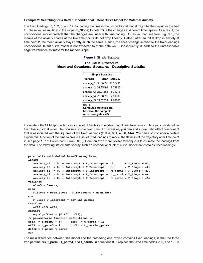
The fixed loadings (0, 1, 2, 6, and 12) for coding the time in the unconditional model might be the culprit for the badfit. These values multiply to the slope (F_Slope) to determine the changes at different time lapses. As a result, theunconditional model predicts that the changes are linear with time coding. But as you can see from Figure 1, themeans of the anxiety scores at the five time points do not drop linearly. Rather, after an initial drop in anxiety attime point 2, the mean anxiety stays pretty much the same. Hence, the linear change implied by the fixed-loadingsunconditional latent curve model is not expected to fit the data well. Consequently, it leads to the unreasonablenegative variance estimate for the random slope.

Figure 1 Simple Statistics

The CALIS ProcedureMean and Covariance Structures: Descriptive Statistics

The CALIS ProcedureMean and Covariance Structures: Descriptive Statistics

Simple Statistics

Variable Mean Std Dev

anxiety_t1 38.86555 10.12231

anxiety_t2 31.25494 9.79926

anxiety_t3 28.94361 8.31015

anxiety_t4 28.38095 7.91909

anxiety_t5 29.02632 9.02868

NOTE:Computed statistics arebased on the completerecords only (N = 42).

Fortunately, the SEM approach gives you a lot of flexibility in modeling nonlinear trajectories. It lets you consider otherfixed loadings that reflect the nonlinear curve over time. For example, you can add a quadratic effect componentthat is associated with the squares of the fixed loadings (that is, 0, 1, 4, 36, 144). You can also consider a certainexponential function of the time to create a set of fixed loadings to model the flatness of the trajectory after time point2 (see page 107 of Bollen and Curran 2006). Here, an even more flexible technique is to estimate the loadings fromthe data. The following statements specify such an unconditional latent curve model that contains freed loadings:

proc calis method=fiml basefit=kang_base;lineqs

anxiety_t1 = 0. * Intercept + F_Intercept + 0. * F_Slope + e1,anxiety_t2 = 0. * Intercept + F_Intercept + 1. * F_Slope + e2,anxiety_t3 = 0. * Intercept + F_Intercept + t_parm3 * F_Slope + e3,anxiety_t4 = 0. * Intercept + F_Intercept + t_parm4 * F_Slope + e4,anxiety_t5 = 0. * Intercept + F_Intercept + t_parm5 * F_Slope + e5;


meanF_Slope = mean_slope, F_Intercept = mean_int;


testfunceff3 eff4 eff5;

simtestequal_effect = [diff1 diff2];

/* parameteric function definitions */eff3 = t_parm3 - 1; eff4 = t_parm4 - 1;eff5 = t_parm5 - 1; diff1 = t_parm3-t_parm4;diff2 = t_parm4-t_parm5;run;

The main difference between this model and the preceding one, which contains fixed loadings, is that the threefree parameters, t_parm3, t_parm4, and t_parm5, in equations 3–5 replace the fixed time codes 2, 6, and 12. In

5

addition to the observed nonlinear trajectory of the mean anxiety, there are other reasons to believe that the currentfreed-loadings unconditional model is more reasonable.

First of all, the coding for the last three time points at 2, 6, and 12 is the number of months for the corrected age of theinfants. However, the “0” code for time point 1 was actually not two months before the third time point. It occurred atsome time during the hospitalization. The “1” code for time point 2 was actually not one month before the third timepoint, either. It was the time when the preterm infant was discharged from the hospital.

Knowing these facts, you can interpret the freed loadings as follows. The mean of the random slope (F_Slope) isinterpreted as the change in the mean anxiety level at discharge. The freed loadings in t_parm3, t_parm4, andt_parm5 represent the multiples of this initial change at 2, 6, and 12 months of corrected age of the infants. If themean anxiety level stays the same at each of these time points after discharge, then the estimates of these loadingsshould all be close to 1. If the mean anxiety level is decreasing over time, then these loadings should get larger overtime (assuming that the mean of F_Slope is negative). Hence, the estimates of t_parm3, t_parm4, and t_parm5 stillprovide useful information about the trajectory when you do not have a hypothesized curve pattern in advance.

Table 1 shows that the freed-loadings unconditional model fits much better than the model that contains fixed loadings.For example, the chi-square model fit test is not significant at the 0.05 ˛-level. RMSEA and SRMR are much reduced,and the CFI value is higher than 0.9. Smaller AIC and SBC values also indicate that this is a better model than thefixed-loadings model.

More importantly, you can interpret the estimates of this model meaningfully. The random intercept has a mean of39.48 and a variance of 97.37 (standard deviation is about 10). This shows considerable variability in the initial anxietylevels of the mothers. The mean slope, –8.38, represents the drop in the mean anxiety level at discharge from thehospital. This drop has a variance of 61.59, so the standard deviation is about 8. The negative covariance estimatemeans that the random intercept and the random slope are negatively related. The higher the initial anxiety, thesmaller the slope. Because the mean slope is negative in the current model, this actually means that patients whohave higher initial anxiety would see their anxiety drop more at the time of discharge. This covariance translates to acorrelation of –0.746, which is pretty strong. The common error variance is estimated at 35.96, which is considerablysmaller than those obtained from the baseline and fixed-loadings models.

Figure 2 shows the loading estimates at time points 3–5 in the equations.

Figure 2 Linear Equations

The CALIS ProcedureMean and Covariance Structures: Full Information Maximum Likelihood Estimation


Linear Equations

anxiety_t1 = 0 Intercept + 1.0000 F_Intercept + 0 F_Slope + 1.0000 e1

anxiety_t2 = 0 Intercept + 1.0000 F_Intercept + 1.0000 F_Slope + 1.0000 e2

anxiety_t3 = 0 Intercept + 1.0000 F_Intercept + 1.1940 (**) F_Slope + 1.0000 e3



All these loadings are significant at the 0.01 ˛-level. They are all close to 1 and show a slightly decreasing trend. Thismeans that the anxiety level at the second month of corrected age dropped a little more but then slowly climbed uptoward the same level as at discharge. You can test some interesting hypotheses about these loading estimates byusing the TESTFUNC and SIMTEST statements.

In the TESTFUNC statement, you test whether parametric functions eff3, eff4, and eff5 are significantly different from0. These functions are defined as programming statements toward the end of the specification. For example, eff3 isdefined as the difference between the constant 1 and the loading at time point 3. Hence, the TESTFUNC statementtests whether the loading estimates are significantly different from 1. Figure 3 shows that each loading estimate is notsignificantly different from 1. This implies that the patients’ anxiety levels stay pretty much the same after discharge.

6

Figure 3 Tests for Parametric Functions

Tests for Parametric Functions

ParametricFunction Estimate

StandardError t Value Pr > |t|

eff3 0.19396 0.11617 1.6696 0.0950

eff4 0.15397 0.12290 1.2528 0.2103

eff5 0.12122 0.11944 1.0149 0.3102

In the SIMTEST statement, the parametric functions diff1=0 and diff2=0 are tested simultaneously. In the program-ming statements, diff1 is further defined as the difference between the first two freed loadings, and diff2 is defined asthe difference between the last two freed loadings. The simultaneous test (diff1=0 and diff2=0) is for the hypothesisof equal loadings for time points 3–5. Figure 4 shows nonsignificant results, meaning that you cannot reject thehypothesis that these loadings are the same in the general population.

Figure 4 Simultaneous Tests

Simultaneous Tests

SimultaneousTest

ParametricFunction

FunctionValue DF Chi-Square p Value

equal_effect 2 0.47342 0.7892

diff1 0.03999 1 0.13588 0.7124

diff2 0.03275 1 0.08720 0.7678

Considering all these results about the freed loadings, you might wonder whether a model that defines only a singledrop in anxiety level at discharge would be a better model. You can specify such a constant-change model by usingthe following statements:

proc calis data=kangaroo_sum method=fiml basefit=kang_base;lineqs

anxiety_t1 = 0. * Intercept + F_Intercept + 0. * F_Slope + e1,anxiety_t2 = 0. * Intercept + F_Intercept + 1. * F_Slope + e2,anxiety_t3 = 0. * Intercept + F_Intercept + 1. * F_Slope + e3,anxiety_t4 = 0. * Intercept + F_Intercept + 1. * F_Slope + e4,anxiety_t5 = 0. * Intercept + F_Intercept + 1. * F_Slope + e5;


meanF_Slope = mean_slope, F_Intercept = mean_int;


run;

The last column of Table 1 shows the estimation results of this model. The estimates of this model are similar to thoseobserved for the model that contains freed loadings. Fit indices that take model parsimony into account (RMSEA,AIC, and SBC) do show that the constant-change model is the best one. However, you might not want to jump to theconclusion that anxiety levels did not change after discharge. First, this model has been derived in an exploratorymanner, so overfitting might be a problem. Second, the insignificant test results of the freed loadings might have beendue to the lack of power in the test. Hence, it would be safer to conclude that this model gives you some workinghypothesis for further testing but that you should interpret your results mainly by using the freed-loadings unconditionalmodel.

Example 3: Conditional Latent Curve Models for Maternal Anxiety

So far, only KC patients have been used in the modeling. To get a more complete picture of the change in anxiety, itwould be useful to also include the patients from the control group. This example includes the control patients andadds a binary variable, trt, that distinguishes the KC patients from the control patients in the analysis.

You could study the group differences in two ways. One way is to use a multiple-group setting that uses two constrainedlatent curves for the two groups. The other is to add trt as a covariate to a single latent curve model. There are pros

7

and cons to both strategies. This example adopts the latter strategy to demonstrate the conditional latent curve model.Henceforth, trt is referred to as the treatment covariate in the model.

What would be a useful baseline model for this conditional model? You could use the baseline model from Example 1,but it does not include the treatment covariate. Therefore, it constrains the KC group and the control group to haveexactly the same no-growth curve in the baseline model. Alternatively, you can consider a baseline model that allowsseparate no-growth curves for the two groups of patients, as specified by the following statements:

proc calis method=fiml outfit=cond_base;lineqs

anxiety_t1 = 0. * Intercept + F_Intercept + e1,anxiety_t2 = 0. * Intercept + F_Intercept + e2,anxiety_t3 = 0. * Intercept + F_Intercept + e3,anxiety_t4 = 0. * Intercept + F_Intercept + e4,anxiety_t5 = 0. * Intercept + F_Intercept + e5,F_Intercept = mean_Int * Intercept + trteff * trt + e6;

variancee1-e5 = 5 * errv, e6 = var_Int;

run;

The most distinctive feature of this baseline model is that it includes the treatment covariate in a new equation for therandom intercept F_Intercept, as shown in the last equation of the LINEQS statement. In this equation, the mean_intparameter serves as an overall mean anxiety for all patients. Because the treatment covariate, trt, is binary, the trteffparameter represents the treatment effect of KC as compared with the control. The variance of e6, labeled as var_Intin the VARIANCE statement, is the conditional variance of the random intercept. In sum, the current specificationallows two different no-growth curves: one for the treatment group and one for the control group. The difference inelevation of the two conditions is characterized by the trteff parameter.

You specify the conditional latent curve model that you want to evaluate by using the following statements:

proc calis method=fiml basefit=cond_base;lineqs

anxiety_t1 = 0. * Intercept + F_Intercept + 0. * F_Slope + e1,anxiety_t2 = 0. * Intercept + F_Intercept + 1. * F_Slope + e2,anxiety_t3 = 0. * Intercept + F_Intercept + t_parm3 * F_Slope + e3,anxiety_t4 = 0. * Intercept + F_Intercept + t_parm4 * F_Slope + e4,anxiety_t5 = 0. * Intercept + F_Intercept + t_parm5 * F_Slope + e5,F_Intercept = mean_Int * Intercept + trteff * trt + e6,F_Slope = mean_Slope * Intercept + trtTimeInt * trt + e7;

variancee1-e5 = 5 * errv, e6 = var_Int, e7 = var_Slope;

cove6 e7 = cov_int_slope;

testfunceff3 eff4 eff5;

simtestequal_effect = [diff1 diff2];

/* parameteric function definitions */diff1 = t_parm3-t_parm4; diff2 = t_parm4-t_parm5;eff3 = t_parm3 - 1; eff4 = t_parm4 - 1;eff5 = t_parm5 - 1;

run;

Like the unconditional latent curve model, the current target conditional model adds the random slope F_Slope topredict the anxiety levels over time. The loadings t_parm3–t_parm5 at time points 3–5 are free parameters to modelthe latent curve with an arbitrary shape. They have the same interpretations as their counterparts in the unconditionalmodel. That is, they represent the multiples of the initial change (when being discharged) at 2, 6, and 12 months ofcorrected ages. Other important features of the model specification are explained as follows:

� The trteff parameter represents the fixed treatment effect that contrasts the KC group with the control group.

� The trtTimeInt parameter represents the fixed interaction effect of treatment and time (freed loadings).

8

� The VARIANCE statement labels the conditional variance of the random intercept as var_Int and the conditionalvariance of random slope as var_Slope.

� The TESTFUNC and SIMTEST statements define statistical tests for testing, respectively, whether the loadingsare different from 1 or whether the loadings are the same.

There are 93 complete observations and 71 incomplete observations in the analysis. Table 2 summarizes theestimation results.

Table 2 Fit Summary of Various Conditional Models


Baseline Freed Loadings

Chi-square 281.12 43.32df 21 14p-value <0.0001 <0.0001RMSEA 0.275 0.113SRMR 0.319 0.097CFI – 0.887IFI – 0.769AIC 5193.48 4969.68SBC 5212.08 5009.98

TreatmentEffect (trteff) –0.465 (p=0.714) –2.121 (p=0.300)Interaction with time (trtTimeInt) 1.601 (p=0.309)

Random interceptMean 33.170 (p<0.0001) 41.472 (p<0.0001)Variance 40.535 (p<0.0001) 126.488 (p<0.0001)

Random slopeMean –9.073 (p<0.0001)Variance 60.122 (p<0.0001)

Covariance –70.749 (p<0.0001)Correlation –0.803 (p<0.0001)Error variance 88.333 (p<0.0001) 41.723 (p<0.0001)


The target conditional latent curve model (last column) shows the appropriate fit of the data. RMSEA (0.113) andSRMR (0.097) seem to be acceptable as a crude model for the data. The CFI value is 0.887, and the IFI value is 0.769.These values are not too bad, considering that they could have been higher if you had chosen a more restrictivebaseline model that assumed the same no-growth curve for the two groups of patients.

A novel feature in this conditional model is the inclusion of the treatment covariate that differentiates the KC groupfrom the control group. The estimate of trteff is –2.121, indicating a slightly lower anxiety level for the KC condition.However, this estimate is not significant (p = 0.300). Neither is the interaction of treatment and time (p = 0.309 for thetrtTimeInt estimate). Interpretations of the random intercept and random slope parameters are similar to those forthe unconditional model, and therefore they are not repeated here. The main conclusion is that the KC group and thecontrol group did not differ in their anxiety levels at all time points.

Figure 5 shows the estimated equations, including those for freed loadings. Figure 6 shows that all loading estimatesare significantly different from 1 at the 0.05 ˛-level. This is different from the corresponding results for the unconditionalmodel where you find no significance difference. Apparently, the tests here gain more power by including the patientsfrom the control group.

9




Linear Equations

anxiety_t1 = 0 Intercept + 1.0000 F_Intercept + 0 F_Slope + 1.0000 e1

anxiety_t2 = 0 Intercept + 1.0000 F_Intercept + 1.0000 F_Slope + 1.0000 e2




F_Intercept = 41.4725 (**) Intercept + -2.1219 (ns) trt + 1.0000 e6

F_Slope = -9.0725 (**) Intercept + 1.6012 (ns) trt + 1.0000 e7

Figure 6 Tests for Parametric Functions

Tests for Parametric Functions

ParametricFunction Estimate

StandardError t Value Pr > |t|

eff3 0.36254 0.09611 3.7719 0.0002

eff4 0.35503 0.09976 3.5590 0.0004

eff5 0.22828 0.09377 2.4346 0.0149

Figure 7 shows the simultaneous test of the equality of the freed loadings. Again, it appears that all these loadingscould have been the same in the population.

Figure 7 Simultaneous Tests

Simultaneous Tests

SimultaneousTest

ParametricFunction

FunctionValue DF Chi-Square p Value

equal_effect 2 3.35073 0.1872

diff1 0.00751 1 0.00916 0.9238

diff2 0.12675 1 2.32297 0.1275

Example 4: Multivariate Latent Curve Models for Maternal Anxiety and Worry

In theory, you can fit as many responses as you want in a latent curve model. In addition to the anxiety measures, thisexample includes the worry measures (worry about child’s health) and demonstrates the so-called multivariate latentcurve model.

First, you use the following statements to set up a baseline conditional model that assumes no change in either theanxiety level or the worry level over time:

proc calis method=fiml outfit=mult_base;lineqs

anxiety_t1 = 0. * Intercept + F_Int_anxi + e1,anxiety_t2 = 0. * Intercept + F_Int_anxi + e2,anxiety_t3 = 0. * Intercept + F_Int_anxi + e3,anxiety_t4 = 0. * Intercept + F_Int_anxi + e4,anxiety_t5 = 0. * Intercept + F_Int_anxi + e5,worry_t1 = 0. * Intercept + F_Int_worry + e6,worry_t2 = 0. * Intercept + F_Int_worry + e7,worry_t3 = 0. * Intercept + F_Int_worry + e8,worry_t4 = 0. * Intercept + F_Int_worry + e9,worry_t5 = 0. * Intercept + F_Int_worry + e10,F_Int_anxi = mean_Int_anxi * Intercept + trteff_anxi * trt + e11,F_Int_worry = mean_Int_worry * Intercept + trteff_worry * trt + e12;

10

variancee1-e5 = 5 * errv_anxi, e6-e10 = 5 * errv_worry,e11 = var_Int_anxi, e12 = var_Int_worry;

cove11 e12 = cov_int;

run;

The basic idea of this baseline model is similar to that in Example 3, except that equations are now duplicated for theworry variable. Notice that the trt variable is also included as a covariate in the last two equations. The elevations inanxiety and worry, though assumed to be flat over time, are allowed to be different for the KC and control groups in thisbaseline model. A new specification here is the covariance of e11 and e12 in the COV statement. This specificationallows the random intercepts to be correlated.

You specify the target multivariate (conditional) model by using the following statements:

proc calis method=fiml basefit=mult_base;lineqs

anxiety_t1 = 0. * Intercept + F_Int_anxi + 0. * F_Slope_anxi + e1,anxiety_t2 = 0. * Intercept + F_Int_anxi + 1. * F_Slope_anxi + e2,anxiety_t3 = 0. * Intercept + F_Int_anxi + t3_anxi * F_Slope_anxi + e3,anxiety_t4 = 0. * Intercept + F_Int_anxi + t4_anxi * F_Slope_anxi + e4,anxiety_t5 = 0. * Intercept + F_Int_anxi + t5_anxi * F_Slope_anxi + e5,worry_t1 = 0. * Intercept + F_Int_worry + 0. * F_Slope_worry + e6,worry_t2 = 0. * Intercept + F_Int_worry + 1. * F_Slope_worry + e7,worry_t3 = 0. * Intercept + F_Int_worry + t3_worry * F_Slope_worry + e8,worry_t4 = 0. * Intercept + F_Int_worry + t4_worry * F_Slope_worry + e9,worry_t5 = 0. * Intercept + F_Int_worry + t5_worry * F_Slope_worry + e10,F_Int_anxi = mean_Int_anxi * Intercept + trteff_anxi * trt + e11,F_Int_worry = mean_Int_worry * Intercept + trteff_worry * trt + e12,F_Slope_anxi = mean_Slope_anxi * Intercept + trtTimeInt_anxi * trt + e13,F_Slope_worry = mean_Slope_worry * Intercept + trtTimeInt_worry * trt + e14;

variancee1-e5 = 5 * errv_anxi, e6-e10 = 5 * errv_worry,e11 = var_Int_anxi, e12 = var_Int_worry,e13 = var_Slope_anxi, e14 = var_Slope_worry;

cove11 e12 = cov_int, e13 e14 = cov_slope,e11 e13 = cov_int_slope_anxi, e12 e14 = cov_int_slope_worry,e11 e14 = cov_int_anxi_slope_worry, e12 e13 = cov_slope_anxi_int_worry;

run;

Essentially, you add the random slopes for the anxiety and worry variables into the system of equations just asyou did for the single-response latent curve model in Example 3. Interpretations of the multivariate model would besimilar to that of the univariate counterpart, such as that in Example 3. Now you just need to interpret more responsevariables from the estimation results.

Additional parameters in this multivariate model might need more explanation. In the COV statement, you spec-ify the covariance between the random slope and random intercept for each stress measure, respectively, ascov_int_slope_anxi and cov_int_slope_worry. This is the same practice that you used for the univariate case inExample 3. In addition, the COV statement specifies cross-covariances among the random intercepts and slopesbetween the two stress measures. For example, the covariance of e11 and e12 is labeled as cov_int, which is theconditional covariance between the two random intercepts given the treatment. The covariance of e11 and e14 islabeled as cov_int_anxi_slope_worry, which is the conditional covariance between the random intercept of anxietyand the random slope of worry given the treatment, and so on.

There are 92 complete observations and 72 incomplete observations in the analysis. Table 3 summarizes the mainestimation results.

11

Table 3 Fit Summary of Multivariate Latent Curve Models for MaternalAnxiety and Worry


Baseline Freed Loadings

Chi-square 574.30 132.15df 66 49p-value <0.0001 <0.0001RMSEA 0.217 0.102SRMR 0.253 0.087CFI – 0.836IFI – 0.690AIC 9401.60 8993.45SBC 9435.70 9080.24

AnxietyTreatmentEffect –0.375 (p=0.769) –2.117 (p=0.300)Interaction with time 1.597 (p=0.307)Random interceptMean 33.317 (p<0.0001) 41.468 (p<0.0001)Variance 42.037 (p<0.0001) 126.395 (p<0.0001)Random slopeMean –8.978 (p<0.0001)Variance 59.456 (p<0.0001)Covariance(Int,Slope) –70.423 (p<0.0001)Error variance 87.971 (p<0.0001) 41.797 (p<0.0001)

WorryTreatmentEffect –1.095 (p=0.234) –0.006 (p=0.996)Interaction with time –1.147 (p=0.105)Random interceptMean 17.123 (p<0.0001) 20.380 (p<0.0001)Variance 26.221 (p<0.0001) 47.086 (p<0.0001)Random slopeMean –3.180 (p<0.0001)Variance 10.312 (p=0.0006)Covariance(Int,Slope) –15.306 (p<0.0001)Error variance 27.482 (p<0.0001) 14.849 (p<0.0001)

Correlations between Slopes and InterceptsInt and slope of anxiety –0.804(p<0.0001)Int and slope of worry –0.684(p<0.0001)Cross-intercepts 0.842 (p<0.0001) 0.628(p<0.0001)Cross-slopes 0.427(p=0.0006)Int-anxiety and slope-worry –0.432(p<0.0001)Int-worry and slope-anxiety –0.379(p=0.0003)


With RMSEA = 0.102 and SRMR = 0.087, the multivariate model seems to have an appropriate fit of the data. TheCFI value is 0.836, and the IFI value is 0.690, which are not very good; they would have appeared to be better if youhad used a more restrictive baseline model (for example, a baseline model that assumed the same latent curve forthe two variables and for all the treatment conditions).

Although the numerical estimates are different, the anxiety and worry variables have similar patterns regarding the

12

random intercepts, random slopes, and treatment effects. First, being in the KC group or the control group doesnot result in different anxiety and worry levels, because the treatment effects, –2.1166 and –0.00633, on the twomeasures are both insignificant. The interaction effects, 1.597 and –1.147, for these measures, respectively, are alsoinsignificant.

The means of random slopes are –8.98 and –3.28 for the anxiety and worry measures, respectively. Therefore, thesevalues indicate that generally the patients in both the KC and control groups have lower anxiety and worry levels atdischarge. Finally, the random intercept and random slope in each stress measure are negatively correlated. Thisconfirms the previous results that a higher initial level of anxiety or worry tends to lead to a greater decrease in anxietyor worry at discharge. The same negative correlations (–0.432 and –0.379) are also observed between random slopeand random intercept in cross measures.

The estimation of correlations shows that the random intercepts between the two stress measures are positivelycorrelated (0.628). This means that patients who have a high initial anxiety level also tend to have a high initial worrylevel. The strong correlation (0.427) of the random slopes between the two stress measures suggests that patientswho have a greater decrease in their anxiety level at discharge (time point 2) also tend to have a greater decrease intheir worry level at discharge.

Figure 8 displays the equation output from the CALIS procedure. All the freed loadings are statistical significant. Itseems that both sets of loadings for the two measures stay pretty much the same at time points 3–5. To conservespace, no significance tests are conducted here. Notice that the magnitudes of these loadings are not comparablebetween measures, because measures could be based on quite different scales.




Linear Equations

anxiety_t1 = 0 Intercept + 1.0000 F_Int_anxi + 0 F_Slope_anxi + 1.0000 e1

anxiety_t2 = 0 Intercept + 1.0000 F_Int_anxi + 1.0000 F_Slope_anxi + 1.0000 e2

anxiety_t3 = 0 Intercept + 1.0000 F_Int_anxi + 1.3723 (**) F_Slope_anxi + 1.0000 e3



worry_t1 = 0 Intercept + 1.0000 F_Int_worry + 0 F_Slope_worry + 1.0000 e6

worry_t2 = 0 Intercept + 1.0000 F_Int_worry + 1.0000 F_Slope_worry + 1.0000 e7

worry_t3 = 0 Intercept + 1.0000 F_Int_worry + 1.4907 (**) F_Slope_worry + 1.0000 e8



F_Int_anxi = 41.4682 (**) Intercept + -2.1166 (ns) trt + 1.0000 e11

F_Int_worry = 20.3801 (**) Intercept + -0.00633 (ns) trt + 1.0000 e12

F_Slope_anxi = -8.9780 (**) Intercept + 1.5967 (ns) trt + 1.0000 e13

F_Slope_worry = -3.1799 (**) Intercept + -1.1467 (ns) trt + 1.0000 e14

Example 5: Latent Curve Models for Latent Factors

Latent curve modeling is not limited to modeling the trajectories of measured variables. It can also model thetrajectories of latent factors. This example considers such a model for the worry measures.

Recall that seven items were used to assess worry level. Example 4 uses the sum scores of these seven items asan overall measure. However, there are two disadvantages to using the sum scores. The first is the missing dataproblem, which occurs quite often in practice. When you have missing values, computing sum scores must involvesome ad hoc imputations. Unfortunately, ad hoc imputations are often biased. Multiple-imputation methods mightwork well in such cases, but they could be very time-consuming (see Yung and Zhang 2011). Second, computing sumscores assumes that each item contributes equally to the measurement of the underlying factor. Hence, sum scoresmight not be statistically optimum for representing the underlying construct. Instead of using sum scores, a possibleremedy is to do a factor analysis at each time point and then use the estimated factor scores instead. The problemwith this strategy is that factor scores from different time points are based on separate factor analyses, so they mightbe defined quite differently at different time points.

13

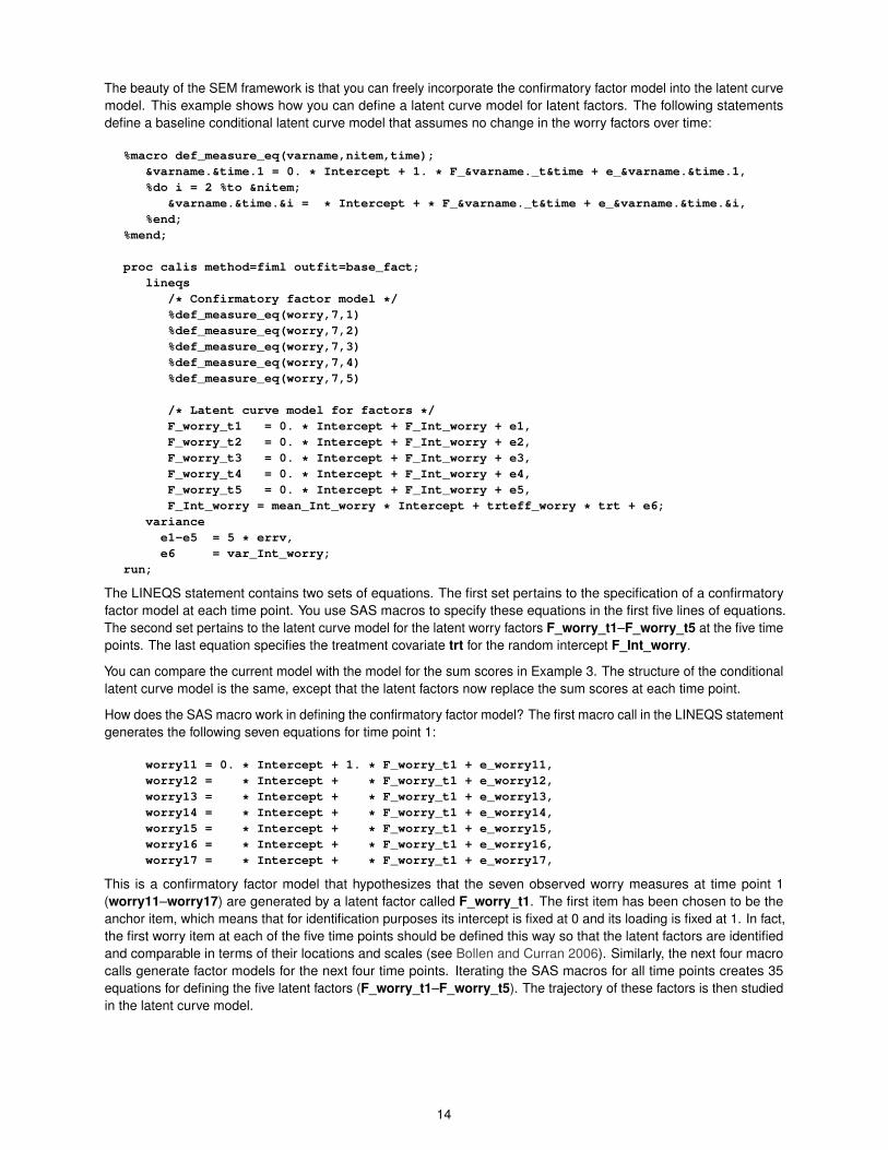
The beauty of the SEM framework is that you can freely incorporate the confirmatory factor model into the latent curvemodel. This example shows how you can define a latent curve model for latent factors. The following statementsdefine a baseline conditional latent curve model that assumes no change in the worry factors over time:

%macro def_measure_eq(varname,nitem,time);&varname.&time.1 = 0. * Intercept + 1. * F_&varname._t&time + e_&varname.&time.1,%do i = 2 %to &nitem;

&varname.&time.&i = * Intercept + * F_&varname._t&time + e_&varname.&time.&i,%end;

%mend;

proc calis method=fiml outfit=base_fact;lineqs

/* Confirmatory factor model */%def_measure_eq(worry,7,1)%def_measure_eq(worry,7,2)%def_measure_eq(worry,7,3)%def_measure_eq(worry,7,4)%def_measure_eq(worry,7,5)

/* Latent curve model for factors */F_worry_t1 = 0. * Intercept + F_Int_worry + e1,F_worry_t2 = 0. * Intercept + F_Int_worry + e2,F_worry_t3 = 0. * Intercept + F_Int_worry + e3,F_worry_t4 = 0. * Intercept + F_Int_worry + e4,F_worry_t5 = 0. * Intercept + F_Int_worry + e5,F_Int_worry = mean_Int_worry * Intercept + trteff_worry * trt + e6;

variancee1-e5 = 5 * errv,e6 = var_Int_worry;

run;

The LINEQS statement contains two sets of equations. The first set pertains to the specification of a confirmatoryfactor model at each time point. You use SAS macros to specify these equations in the first five lines of equations.The second set pertains to the latent curve model for the latent worry factors F_worry_t1–F_worry_t5 at the five timepoints. The last equation specifies the treatment covariate trt for the random intercept F_Int_worry.

You can compare the current model with the model for the sum scores in Example 3. The structure of the conditionallatent curve model is the same, except that the latent factors now replace the sum scores at each time point.

How does the SAS macro work in defining the confirmatory factor model? The first macro call in the LINEQS statementgenerates the following seven equations for time point 1:

worry11 = 0. * Intercept + 1. * F_worry_t1 + e_worry11,worry12 = * Intercept + * F_worry_t1 + e_worry12,worry13 = * Intercept + * F_worry_t1 + e_worry13,worry14 = * Intercept + * F_worry_t1 + e_worry14,worry15 = * Intercept + * F_worry_t1 + e_worry15,worry16 = * Intercept + * F_worry_t1 + e_worry16,worry17 = * Intercept + * F_worry_t1 + e_worry17,

This is a confirmatory factor model that hypothesizes that the seven observed worry measures at time point 1(worry11–worry17) are generated by a latent factor called F_worry_t1. The first item has been chosen to be theanchor item, which means that for identification purposes its intercept is fixed at 0 and its loading is fixed at 1. In fact,the first worry item at each of the five time points should be defined this way so that the latent factors are identifiedand comparable in terms of their locations and scales (see Bollen and Curran 2006). Similarly, the next four macrocalls generate factor models for the next four time points. Iterating the SAS macros for all time points creates 35equations for defining the five latent factors (F_worry_t1–F_worry_t5). The trajectory of these factors is then studiedin the latent curve model.

14

Likewise, you specify the target conditional latent curve model by using the following statements:

proc calis method=fiml basefit=base_fact;lineqs

/* Confirmatory Factor Model */%def_measure_eq(worry,7,1)%def_measure_eq(worry,7,2)%def_measure_eq(worry,7,3)%def_measure_eq(worry,7,4)%def_measure_eq(worry,7,5)

/* Latent curve model for factors */F_worry_t1 = 0. * Intercept + F_Int_worry + 0. * F_Slope_worry + e1,F_worry_t2 = 0. * Intercept + F_Int_worry + 1. * F_Slope_worry + e2,F_worry_t3 = 0. * Intercept + F_Int_worry + t_parm3 * F_Slope_worry + e3,F_worry_t4 = 0. * Intercept + F_Int_worry + t_parm4 * F_Slope_worry + e4,F_worry_t5 = 0. * Intercept + F_Int_worry + t_parm5 * F_Slope_worry + e5,F_Int_worry = mean_Int_worry * Intercept + trteff_worry * trt + e6,F_Slope_worry = mean_Slope * Intercept + trtTimeInt_worry * trt + e7;

variancee1-e5 = 5 * errv,e6 = var_Int_worry,e7 = var_Slope_worry;

cove6 e7 = cov_int_slope;

run;

Not surprisingly, the current latent curve model specification has the same structure as the conditional latent curvemodel in Example 3, which is for sum scores. You add the random slope F_Slope_worry and the treatment variabletrt into the model in exactly the same way that you do for the conditional latent curve model for sum scores.

Table 4 summarizes the main estimation results of the baseline model and the latent curve model for the worry factors.The freed-loadings latent curve model has a reasonable fit, as indicated by the RMSEA and SRMR values. The CFIand IFI values are exceedingly small, indicating that the latent curve model is not much better than the baseline model.

As reflected by the insignificance of the treatment effect (–0.009, p = 0.965) and its interaction effect with the time(–0.236, p = 0.060), the KC group and the control group are not different in their patterns of worry level during theperiod of the study. The mean of the random slope is –0.390 (p = 0.003), showing a general decrease in worry level atdischarge. The negative correlation (–0.402) between the random intercept and the random slope echoes a consistentpattern of maternal distress: the higher the initial level, the higher the drop in the distress level at discharge.

Table 4 Fit Summary of Various Conditional Models


Baseline Freed Loadings Correlated Errors

Chi-square 1623.11 1546.97 1296.79df 601 594 566p-value <0.0001 <0.0001 <0.0001RMSEA 0.102 0.099 0.0887SRMR 0.114 0.101 0.0966CFI – 0.068 0.285IFI – 0.036 0.152AIC 13770.23 13708.09 13513.90SBC 14083.32 14042.87 13935.49

TreatmentEffect (trteff) –0.236 (p=0.140) –0.009 (p=0.965) –0.013 (p=0.946)Interaction with time(trtTimeInt)

–0.236 (p=0.060) –0.242 (p=0.065)

Random interceptMean 2.838 (p<0.0001) 3.301 (p<0.0001) 3.326 (p<0.0001)

15

Table 4 continued

Baseline Freed Loadings Correlated Errors

Variance 0.833 (p<0.0001) 0.985 (p<0.0001) 97.670 (p<0.0001)

Random slopeMean –0.390 (p=0.003) –0.417(p=0.001)Variance 0.250 (p<0.0001) 76.477(p=0.001)

Covariance –0.204 (p=0.118) –05209 (p=0.135)Correlation –0.402 (p=0.011) –0.398 (p=0.016)Error variance 0.498 (p<0.0001) 0.339 (p<0.0001) 0.366 (p<0.0001)


Because the worry measures were administered repeatedly, it would be reasonable to assume that responses tothe same items at different time points are correlated beyond what can be explained by the common latent factors.With the SEM approach, you can easily incorporate this idea into the model. To demonstrate, this example assumesthat the residual of each worry item correlates only with the residual of the same item at adjacent time points. Forexample, the residual of worry11 correlates with the residual of worry21, the residual of worry21 correlates with theresidual of worry31, and so on. To specify these correlations, you can add the error covariances of these variablesinto the COV statement of the preceding PROC CALIS model. That is, the COV statement in the preceding codewould become the following:

cove6 e7 = cov_int_slope,e_worry11 e_worry21, e_worry21 e_worry31, e_worry31 e_worry41, e_worry41 e_worry51,e_worry12 e_worry22, e_worry22 e_worry32, e_worry32 e_worry42, e_worry42 e_worry52,e_worry13 e_worry23, e_worry23 e_worry33, e_worry33 e_worry43, e_worry43 e_worry53,e_worry14 e_worry24, e_worry24 e_worry34, e_worry34 e_worry44, e_worry44 e_worry54,e_worry15 e_worry25, e_worry25 e_worry35, e_worry35 e_worry45, e_worry45 e_worry55,e_worry16 e_worry26, e_worry26 e_worry36, e_worry36 e_worry46, e_worry46 e_worry56,e_worry17 e_worry27, e_worry27 e_worry37, e_worry37 e_worry47, e_worry47 e_worry57;

The last column of Table 4 shows the main estimation results. RMSEA is 0.0887, and SRMR is 0.0966; they show areasonable fit of the model. The CFI value (0.283) and IFI value (0.152) are higher than in the preceding model thatdoes not assume correlated errors. However, these indices still appear to be low. This model is not a big improvementover the baseline model chosen in this example. Estimates about the random slope and random intercept have similarpatterns to those of the preceding model. Therefore, there is no need to repeat the interpretations here.

CONCLUSION

This paper illustrates how you can use the SEM approach to model longitudinal data. The main idea is that you canrepresent the random intercept and random slope in longitudinal modeling as latent factors in the SEM approach.After you define these parameters properly in the model, you can benefit from the advantages that the flexible andgeneral SEM framework gives you, including the following:

� flexible nonlinear trajectories, such as freed loadings (estimated time code), piecewise linear trajectory, andmany other nonlinearity specifications (see Bollen and Curran 2006)

� trajectory of latent factors, in addition to that of observed variables. This is especially useful for high-dimensionaldata.

� flexible parameterization in models such as arbitrary linear and nonlinear constraints

� multiple-group models. In multiple-group analysis, you can fit either the same or different models for differentgroups. You can constrain any parameters across groups. In the context of longitudinal data analysis, forexample, you can use multiple-group analysis to test whether there is a difference in the variance of the slopefactor. Such a difference might have very useful substantive meanings.

16

The SEM approach also has some disadvantages, including the following:

� As a general modeling tool, SEM software tends to be harder to use. For simpler and standard mixed models,analytic software such as PROC MIXED, which is dedicated to mixed modeling, is much easier to use.

� The SEM methodology has not been designed specifically for latent curve modeling. Existing SEM methods andtechniques might not be appropriate. For example, choosing a good baseline model for latent curve analysis isa challenge that has not been completely resolved. Although the no-growth model seems to serve as a goodbaseline model for simple unconditional models, it is unclear whether it is suitable for more complex modelssuch as conditional models, possibly combined with latent factor trajectory.

� Somewhat related to the previous point, in SEM you need to generate initial estimates and obtain the finalestimates through iterations. Because the strategy of generating initial estimates in SEM software doesnot consider latent curve modeling specifically, bad initial estimates are possible, and they could lead tononconverged or bad solutions. In the process of writing this paper, the authors encountered some cases(about 10%–20% of the time) in which PROC CALIS converged to bad solutions. By means of the OUTEST=and INEST= options, the problem was solved by fitting another model with similar characteristics (for example,with some fixed loadings) and then feeding the final estimates into the target model as “good” initial values.However, this certainly is a heuristic but not a general solution to all convergence problems.

Despite these disadvantages, the modeling flexibility of the SEM approach has a lot of potential for longitudinal dataanalysis. This potential has not been fully explored. Hopefully, this paper has provided some useful initial steps forapplying this approach by using the CALIS procedure.

REFERENCES

Bollen, K. A. (1989). Structural Equations with Latent Variables. New York: John Wiley & Sons.

Bollen, K. A., and Curran, P. J. (2006). Latent Curve Models: A Structural Equation Perspective. Hoboken, NJ: JohnWiley & Sons.

Chatfield, C. (2003). The Analysis of Time Series: An Introduction. 6th ed. Boca Raton, FL: Chapman & Hall/CRC.

Gao, F., Thompson, P., Xiong, C., and Miller, J. P. (2006). “Analyzing Multivariate Longitudinal Data Using SAS.” InProceedings of the Thirty-First Annual SAS Users Group International Conference, 187–31. Cary, NC: SAS InstituteInc. http://www2.sas.com/proceedings/sugi31/187-31.pdf.

Holditch-Davis, D., White-Traut, R. C., Levy, J. A., O’Shea, T. M., Geraldo, V., and David, R. J. (2014). “MaternallyAdministered Interventions for Preterm Infants in the NICU: Effects on Maternal Psychological Distress andMother-Infant Relationship.” Infant Behavior and Development 37:695–710.

Lu, P.-C., and Pearson, R. (2013). “Modeling Change over Time: A SAS Macro for Latent Growth Curve Modeling.” InProceedings of the SAS Global Forum 2013 Conference. Cary, NC: SAS Institute Inc. http://support.sas.com/resources/papers/proceedings13/452-2013.pdf.

Preacher, K. J., Wichman, A. L., MacCallum, R. C., and Briggs, N. E. (2008). Latent Growth Curve Modeling.Thousand Oaks, CA: Sage Publications.

Verbeke, G., and Molenberghs, G. (2000). Linear Mixed Models for Longitudinal Data. New York: Springer.

Yung, Y.-F., and Zhang, W. (2011). “Making Use of Incomplete Observations in the Analysis of Structural EquationModels: The CALIS Procedure’s Full Information Maximum Likelihood Method in SAS/STAT 9.3.” In Proceed-ings of the SAS Global Forum 2011 Conference. Cary, NC: SAS Institute Inc. http://support.sas.com/resources/papers/proceedings11/333-2011.pdf.

17

http://www2.sas.com/proceedings/sugi31/187-31.pdf

http://support.sas.com/resources/papers/proceedings13/452-2013.pdf




ACKNOWLEDGMENTS

The authors are grateful to Ed Huddleston of the Advanced Analytics Division at SAS Institute Inc. for his valuableassistance in the preparation of this paper.

CONTACT INFORMATION

Your comments and questions are valued and encouraged. Contact the authors:

Xinming An Yiu-Fai Yung Qing YangSAS Institute Inc. SAS Institute Inc. Duke UniversitySAS Campus Drive SAS Campus Drive 307 Trent DriveCary, NC 27513 Cary, NC 27513 Durham, NC [email protected] [email protected] [email protected]

SAS and all other SAS Institute Inc. product or service names are registered trademarks or trademarks of SASInstitute Inc. in the USA and other countries. ® indicates USA registration.

Other brand and product names are trademarks of their respective companies.

18

the sem approach to longitudinal data analysis using the ... · the sem approach to longitudinal...

Documents