the scf-anderson method for a non-linear eigenvalue problem

The SCF-Anderson method for a Non-linear Eigenvalue Problemin Electronic Structure Computations

by

Peng Ni

A Project Report

Submitted to the Faculty

of

WORCESTER POLYTECHNIC INSTITUTE

in Partial Fulfillment of the Requirements for the

Degree of Doctor of Philosophy

in

Mathematical Sciences

by

August 2007

APPROVED:

Dr. Homer Walker, Project Advisor

1

1 Introduction

1.1 Background introduction

In the field of nanomaterials and devices, people often need to identify un-known structures.

Any material has a unique “ground state” — that is, the minimum-energylevel where the material’s electrons remain unless the material is perturbedby external sources. If it is possible to determine a material’s ground state,then it is possible to identify the material itself.

A current approach is to find out the charge density associated with theground state, and this envolves setting up nonlinear eigenvalue problems inthe process.

Dr. Chao Yang from Lawrence Berkeley National Laboratory is working onthis nonlinear eigenvalue problem. He is interested in finding out the proper-ties of a particular existing algorithm, improving the performance of it, anddeveloping alternative approaches if possible.

I got this project topic from Dr. Yang, and worked under the instructionfrom him and my advisor Dr. Walker. Thanks to both of them.

1.2 Problem introduction

In most situations in chemistry, it is legitimate to consider the nuclei as clas-sical objects and as point-like particles with charges (λ1,λ2,...,λp) at positions(x1,x2,...,xp), while treating the electrons as quantum particles. This is theso-called Born-Oppenheimer approximation. In view of this approximation,the determination of the ground state (that is, the state of minimum en-ergy) structure of a molecular system consisting of p nuclei and n electronsamounts to solving a minimization problem. See details in [3].

The specific mathematical problem under this background is to minimize the

2

total energy function:minEtotal(X)s.t. X ′X = Ip

This problem is transformed into a nonlinear eigenvalue problem (the Kohn-Sham equation from [7]):

H(X)X = XΛp

X ′X = Ip,(1)

where the columns of X ∈ Rn×p (p < n) are approximate electron wavefunctions, H ∈ Rn×n is the discrete Hamiltonian and is dependent on X,Λp ∈ Rp×p is a diagonal matrix with the p smallest eigenvalues of H on thediagonal, and Ip ∈ Rp×p is identity matrix. ρ = diag(XX ′) is called thecharge density.

Current approaches to this problem include the Self-Consistent Field (SCF)method [7] and the SCF method accelerated by the Anderson Acceleration[1] (SCF-Anderson).

1.3 Algorithm introduction

In the following, some MATLAB notation is used. In particular, for A ∈Rp×p, diag(A) denotes the vector in Rp the components of which are thediagonal entries of A, and [ ] denotes the “empty” matrix.

1.3.1 The SCF method

Use X ∈ Rn×p from previous iteration to calculate H(X) ∈ Rn×n, and view itas a constant matrix in the current iteration. Find the p smallest eigenvaluesof H(X), and use the corresponding eigenvectors to form the columns of anew X for next iteration.

3

Algorithm 1 SCF Method

Given X ∈ Rn×p, and tol > 0, evaluate H(X) ∈ Rn×n.for iter = 1 to Max iter do

Find the p smallest eigenvalues d ∈ Rp×1 and corresponding eigenvectorsfor H(X) to form columns of X+ ∈ Rn×p.Evaluate ∆ρ = diag(X+X

′+)− diag(XX ′).

Evaluate err = ‖∆ρ‖.Update X ←− X+.if err < tol then

Break.end ifUpdate H(X)←− H(X+).

end for

In practice, the SCF method is less effective than expected: the convergenceis slow, and sometimes it even diverges. So for the following parts of thisreport, we will focus on the SCF-Anderson method outlined in §1.3.2, inwhich SCF is augmented with a certain procedure to improve convergence.

1.3.2 The SCF-Anderson method

Actually, in the formula forH(X), X always appears in the form of diag(XX ′),which is the electron density ρ. Basically, what we need to determine H(X)is only ρ, so for simplicity, we will just use H(ρ) instead from now on.

Based on the SCF method, instead of directly letting ρ+ = diag(X+X′+),

choose ρ+ to be a linear combination of the previous values of ρ to strengthenself-consistency.

4

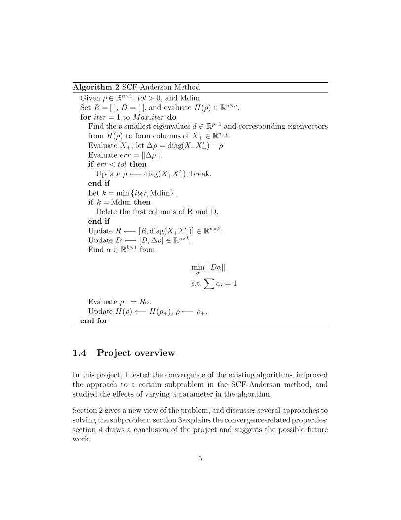
Algorithm 2 SCF-Anderson Method

Given ρ ∈ Rn×1, tol > 0, and Mdim.Set R = [ ], D = [ ], and evaluate H(ρ) ∈ Rn×n.for iter = 1 to Max iter do

Find the p smallest eigenvalues d ∈ Rp×1 and corresponding eigenvectorsfrom H(ρ) to form columns of X+ ∈ Rn×p.Evaluate X+; let ∆ρ = diag(X+X

′+)− ρ

Evaluate err = ||∆ρ||.if err < tol then

Update ρ←− diag(X+X′+); break.

end ifLet k = min {iter,Mdim}.if k = Mdim then

Delete the first columns of R and D.end ifUpdate R←− [R, diag(X+X

′+)] ∈ Rn×k.

Update D ←− [D,∆ρ] ∈ Rn×k.Find α ∈ Rk×1 from

minα||Dα||

s.t.∑

αi = 1

Evaluate ρ+ = Rα.Update H(ρ)←− H(ρ+), ρ←− ρ+.

end for

1.4 Project overview

In this project, I tested the convergence of the existing algorithms, improvedthe approach to a certain subproblem in the SCF-Anderson method, andstudied the effects of varying a parameter in the algorithm.

Section 2 gives a new view of the problem, and discusses several approaches tosolving the subproblem; section 3 explains the convergence-related properties;section 4 draws a conclusion of the project and suggests the possible futurework.

5

2 Implementation of the SCF and SCF-Anderson

method

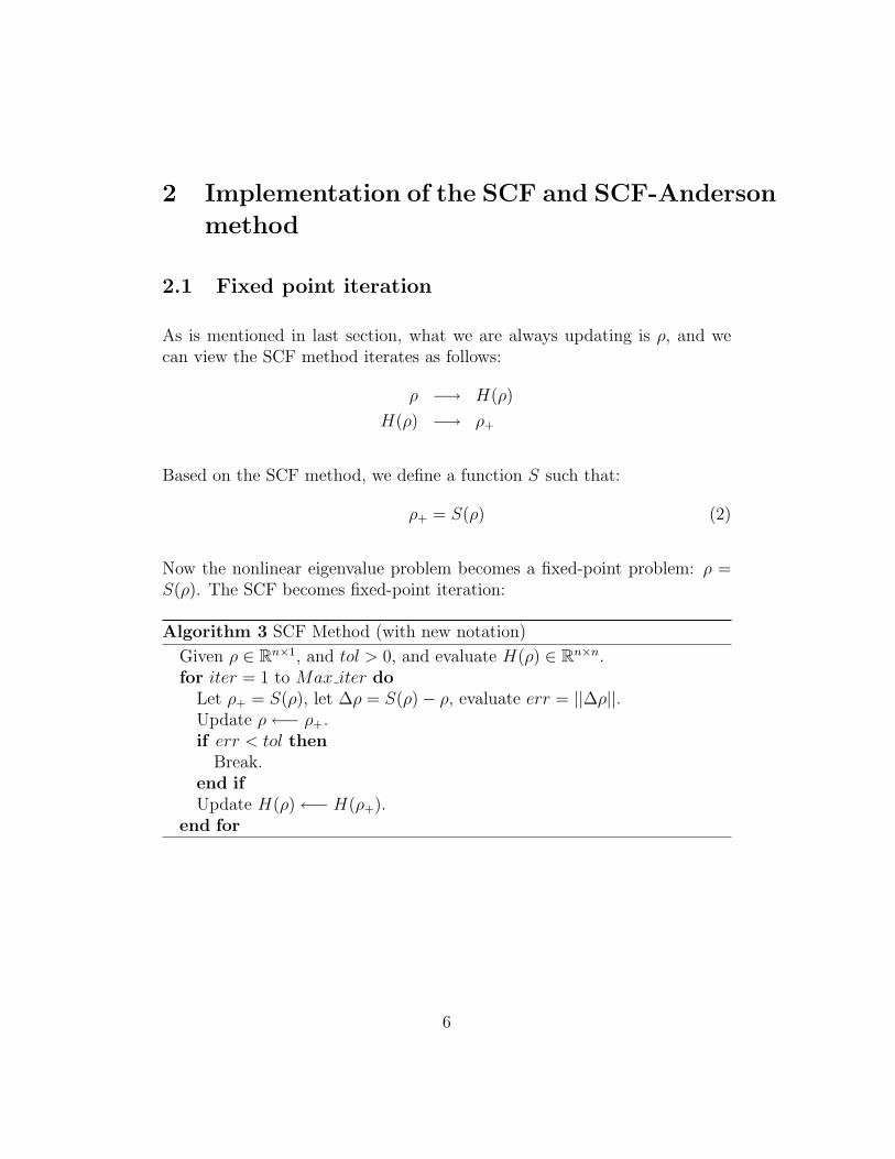
2.1 Fixed point iteration

As is mentioned in last section, what we are always updating is ρ, and wecan view the SCF method iterates as follows:

ρ −→ H(ρ)

H(ρ) −→ ρ+

Based on the SCF method, we define a function S such that:

ρ+ = S(ρ) (2)

Now the nonlinear eigenvalue problem becomes a fixed-point problem: ρ =S(ρ). The SCF becomes fixed-point iteration:

Algorithm 3 SCF Method (with new notation)

Given ρ ∈ Rn×1, and tol > 0, and evaluate H(ρ) ∈ Rn×n.for iter = 1 to Max iter do

Let ρ+ = S(ρ), let ∆ρ = S(ρ)− ρ, evaluate err = ||∆ρ||.Update ρ←− ρ+.if err < tol then

Break.end ifUpdate H(ρ)←− H(ρ+).

end for

6

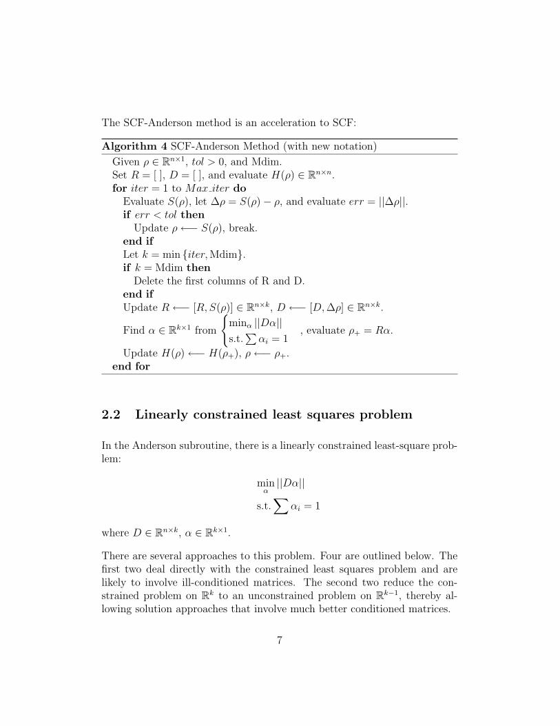
The SCF-Anderson method is an acceleration to SCF:

Algorithm 4 SCF-Anderson Method (with new notation)

Given ρ ∈ Rn×1, tol > 0, and Mdim.Set R = [ ], D = [ ], and evaluate H(ρ) ∈ Rn×n.for iter = 1 to Max iter do

Evaluate S(ρ), let ∆ρ = S(ρ)− ρ, and evaluate err = ||∆ρ||.if err < tol then

Update ρ←− S(ρ), break.end ifLet k = min {iter,Mdim}.if k = Mdim then

Delete the first columns of R and D.end ifUpdate R←− [R, S(ρ)] ∈ Rn×k, D ←− [D,∆ρ] ∈ Rn×k.

Find α ∈ Rk×1 from

{minα ||Dα||s.t.∑αi = 1

, evaluate ρ+ = Rα.

Update H(ρ)←− H(ρ+), ρ←− ρ+.end for

2.2 Linearly constrained least squares problem

In the Anderson subroutine, there is a linearly constrained least-square prob-lem:

minα||Dα||

s.t.∑

αi = 1

where D ∈ Rn×k, α ∈ Rk×1.

There are several approaches to this problem. Four are outlined below. Thefirst two deal directly with the constrained least squares problem and arelikely to involve ill-conditioned matrices. The second two reduce the con-strained problem on Rk to an unconstrained problem on Rk−1, thereby al-lowing solution approaches that involve much better conditioned matrices.

7

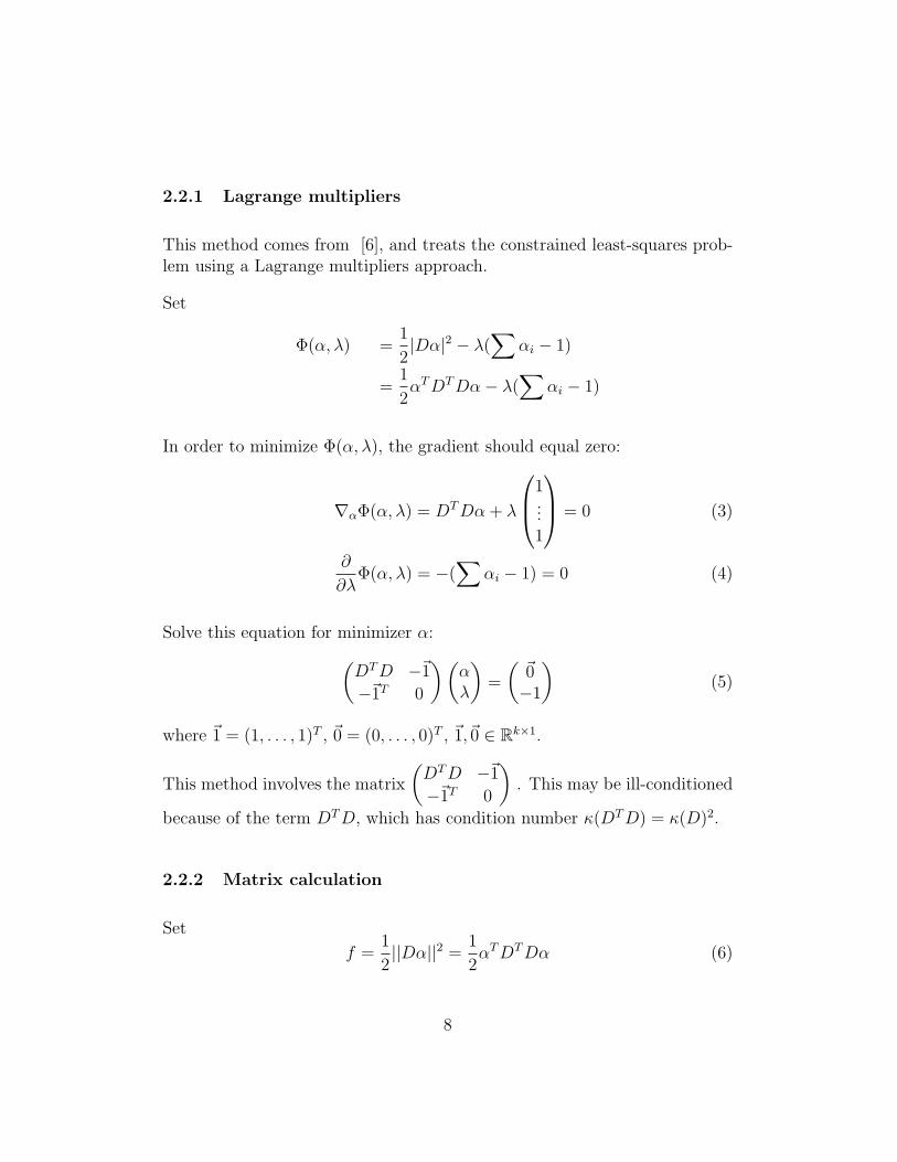
2.2.1 Lagrange multipliers

This method comes from [6], and treats the constrained least-squares prob-lem using a Lagrange multipliers approach.

Set

Φ(α, λ) =1

2|Dα|2 − λ(

∑αi − 1)

=1

2αTDTDα− λ(

∑αi − 1)

In order to minimize Φ(α, λ), the gradient should equal zero:

∇αΦ(α, λ) = DTDα + λ

1...1

= 0 (3)

∂

∂λΦ(α, λ) = −(

∑αi − 1) = 0 (4)

Solve this equation for minimizer α:(DTD −~1−~1T 0

)(αλ

)=

(~0−1

)(5)

where ~1 = (1, . . . , 1)T , ~0 = (0, . . . , 0)T , ~1,~0 ∈ Rk×1.

This method involves the matrix

(DTD −~1−~1T 0

). This may be ill-conditioned

because of the term DTD, which has condition number κ(DTD) = κ(D)2.

2.2.2 Matrix calculation

Set

f =1

2||Dα||2 =

1

2αTDTDα (6)

8

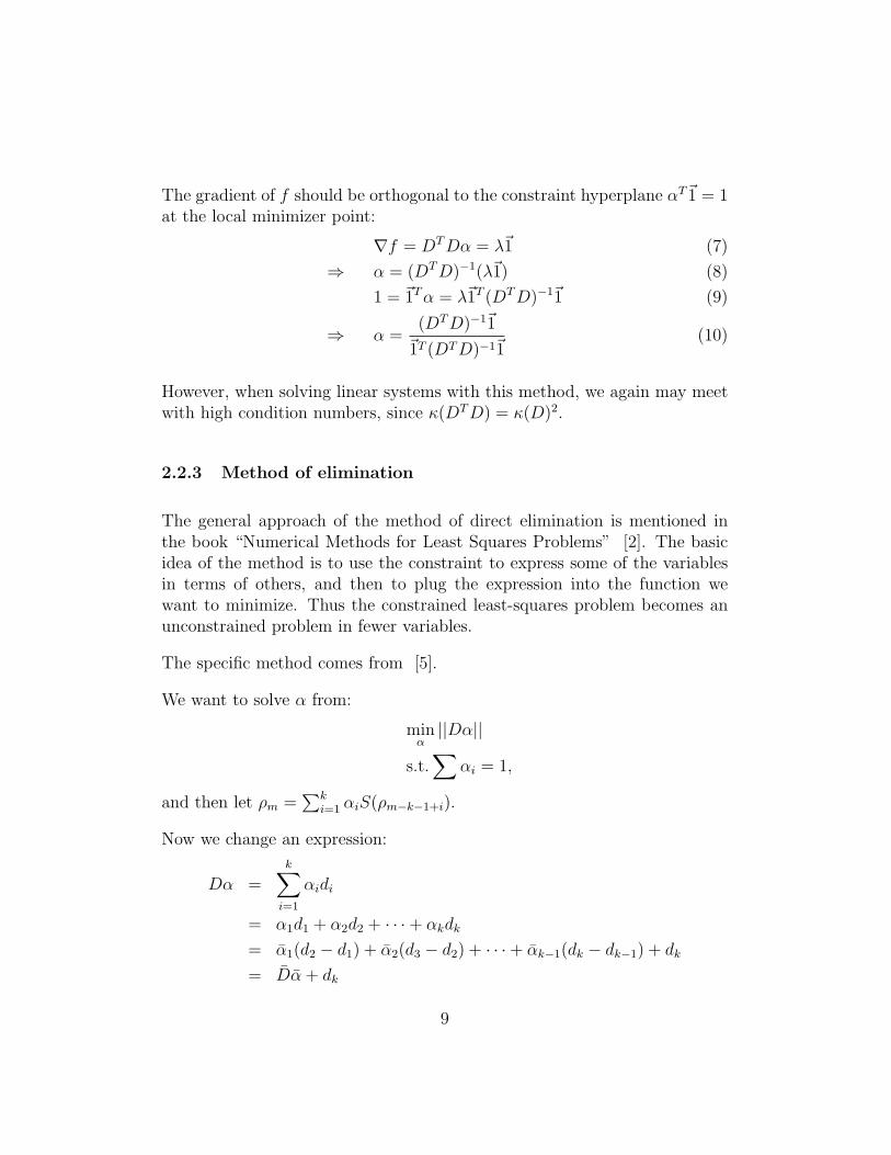
The gradient of f should be orthogonal to the constraint hyperplane αT~1 = 1at the local minimizer point:

∇f = DTDα = λ~1 (7)

⇒ α = (DTD)−1(λ~1) (8)

1 = ~1Tα = λ~1T (DTD)−1~1 (9)

⇒ α =(DTD)−1~1

~1T (DTD)−1~1(10)

However, when solving linear systems with this method, we again may meetwith high condition numbers, since κ(DTD) = κ(D)2.

2.2.3 Method of elimination

The general approach of the method of direct elimination is mentioned inthe book “Numerical Methods for Least Squares Problems” [2]. The basicidea of the method is to use the constraint to express some of the variablesin terms of others, and then to plug the expression into the function wewant to minimize. Thus the constrained least-squares problem becomes anunconstrained problem in fewer variables.

The specific method comes from [5].

We want to solve α from:

minα||Dα||

s.t.∑

αi = 1,

and then let ρm =∑k

i=1 αiS(ρm−k−1+i).

Now we change an expression:

Dα =k∑i=1

αidi

= α1d1 + α2d2 + · · ·+ αkdk

= α1(d2 − d1) + α2(d3 − d2) + · · ·+ αk−1(dk − dk−1) + dk

= Dα + dk

9

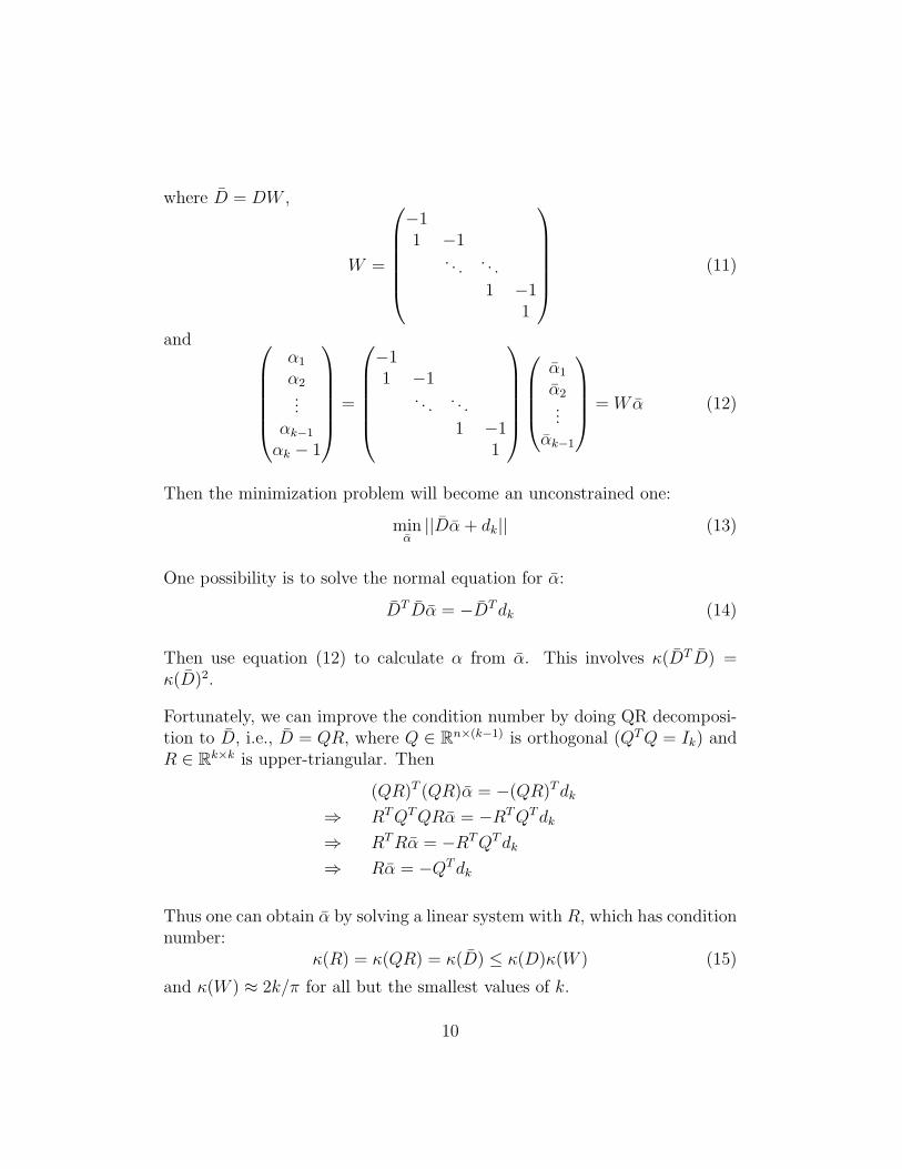
where D = DW ,

W =

−11 −1

. . . . . .

1 −11

(11)

and α1

α2...

αk−1

αk − 1

=

−11 −1

. . . . . .

1 −11

α1

α2...

αk−1

= Wα (12)

Then the minimization problem will become an unconstrained one:

minα||Dα + dk|| (13)

One possibility is to solve the normal equation for α:

DT Dα = −DTdk (14)

Then use equation (12) to calculate α from α. This involves κ(DT D) =κ(D)2.

Fortunately, we can improve the condition number by doing QR decomposi-tion to D, i.e., D = QR, where Q ∈ Rn×(k−1) is orthogonal (QTQ = Ik) andR ∈ Rk×k is upper-triangular. Then

(QR)T (QR)α = −(QR)Tdk

⇒ RTQTQRα = −RTQTdk

⇒ RTRα = −RTQTdk

⇒ Rα = −QTdk

Thus one can obtain α by solving a linear system with R, which has conditionnumber:

κ(R) = κ(QR) = κ(D) ≤ κ(D)κ(W ) (15)

and κ(W ) ≈ 2k/π for all but the smallest values of k.

10

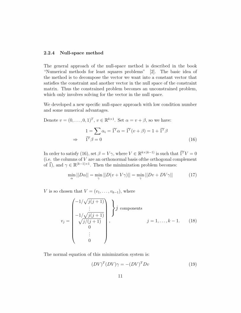
2.2.4 Null-space method

The general approach of the null-space method is described in the book“Numerical methods for least squares problems” [2]. The basic idea ofthe method is to decompose the vector we want into a constant vector thatsatisfies the constraint and another vector in the null space of the constraintmatrix. Thus the constrained problem becomes an unconstrained problem,which only involves solving for the vector in the null space.

We developed a new specific null-space approach with low condition numberand some numerical advantages.

Denote v = (0, . . . , 0, 1)T , v ∈ Rk×1. Set α = v + β, so we have:

1 =∑

αi = ~1Tα = ~1T (v + β) = 1 +~1Tβ

⇒ ~1Tβ = 0 (16)

In order to satisfy (16), set β = V γ, where V ∈ Rk×(k−1) is such that ~1TV = 0(i.e. the columns of V are an orthonormal basis ofthe orthogonal complementof ~1), and γ ∈ R(k−1)×1. Then the minimization problem becomes:

minα||Dα|| = min

γ||D(v + V γ)|| = min

γ||Dv +DV γ|| (17)

V is so chosen that V = (v1, . . . , vk−1), where

vj =

−1/√j(j + 1)...

−1/√j(j + 1)√

j/(j + 1)0...0

,

}j components

j = 1, . . . , k − 1. (18)

The normal equation of this minimization system is:

(DV )T (DV )γ = −(DV )TDv (19)

11

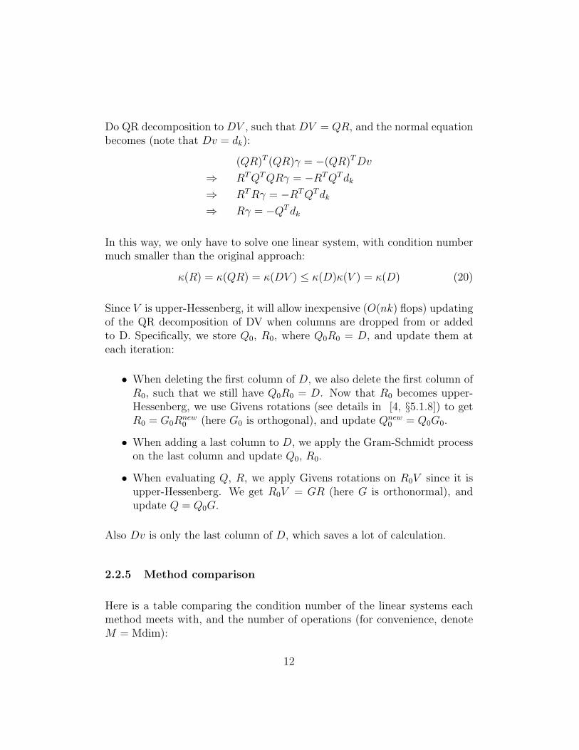
Do QR decomposition to DV , such that DV = QR, and the normal equationbecomes (note that Dv = dk):

(QR)T (QR)γ = −(QR)TDv

⇒ RTQTQRγ = −RTQTdk

⇒ RTRγ = −RTQTdk

⇒ Rγ = −QTdk

In this way, we only have to solve one linear system, with condition numbermuch smaller than the original approach:

κ(R) = κ(QR) = κ(DV ) ≤ κ(D)κ(V ) = κ(D) (20)

Since V is upper-Hessenberg, it will allow inexpensive (O(nk) flops) updatingof the QR decomposition of DV when columns are dropped from or addedto D. Specifically, we store Q0, R0, where Q0R0 = D, and update them ateach iteration:

• When deleting the first column of D, we also delete the first column ofR0, such that we still have Q0R0 = D. Now that R0 becomes upper-Hessenberg, we use Givens rotations (see details in [4, §5.1.8]) to getR0 = G0R

new0 (here G0 is orthogonal), and update Qnew

0 = Q0G0.

• When adding a last column to D, we apply the Gram-Schmidt processon the last column and update Q0, R0.

• When evaluating Q, R, we apply Givens rotations on R0V since it isupper-Hessenberg. We get R0V = GR (here G is orthonormal), andupdate Q = Q0G.

Also Dv is only the last column of D, which saves a lot of calculation.

2.2.5 Method comparison

Here is a table comparing the condition number of the linear systems eachmethod meets with, and the number of operations (for convenience, denoteM = Mdim):

12

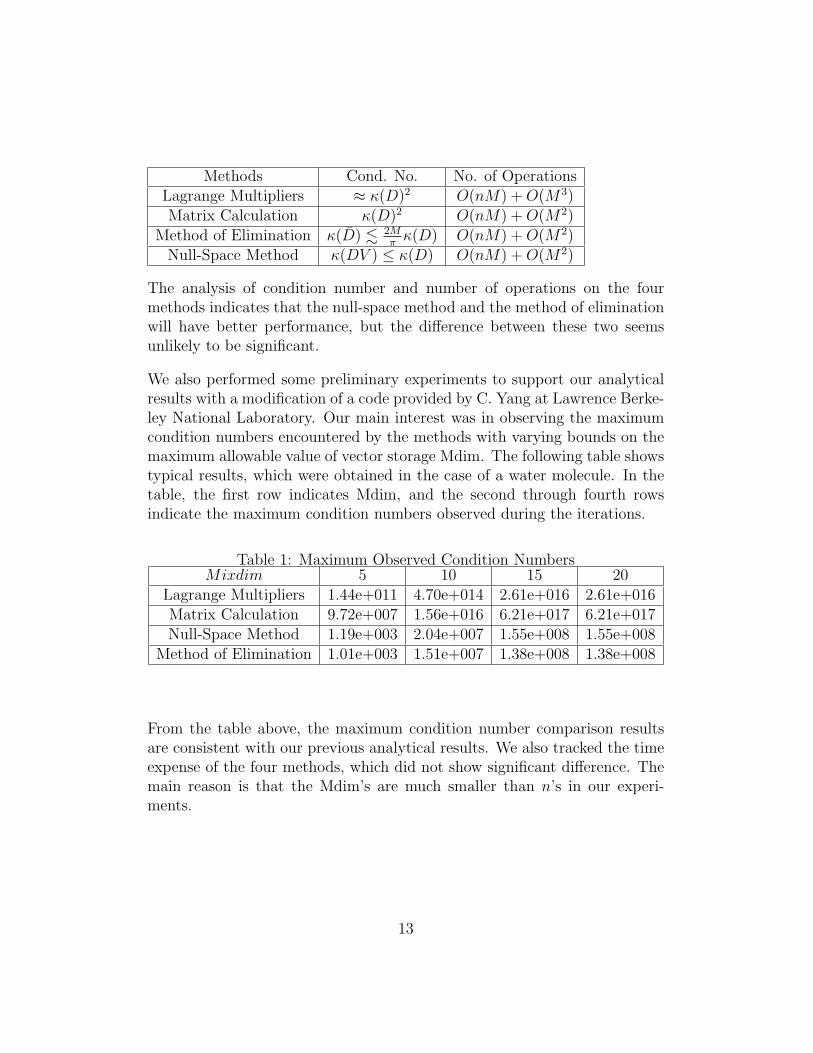
Methods Cond. No. No. of OperationsLagrange Multipliers ≈ κ(D)2 O(nM) +O(M3)Matrix Calculation κ(D)2 O(nM) +O(M2)

Method of Elimination κ(D) . 2Mπκ(D) O(nM) +O(M2)

Null-Space Method κ(DV ) ≤ κ(D) O(nM) +O(M2)

The analysis of condition number and number of operations on the fourmethods indicates that the null-space method and the method of eliminationwill have better performance, but the difference between these two seemsunlikely to be significant.

We also performed some preliminary experiments to support our analyticalresults with a modification of a code provided by C. Yang at Lawrence Berke-ley National Laboratory. Our main interest was in observing the maximumcondition numbers encountered by the methods with varying bounds on themaximum allowable value of vector storage Mdim. The following table showstypical results, which were obtained in the case of a water molecule. In thetable, the first row indicates Mdim, and the second through fourth rowsindicate the maximum condition numbers observed during the iterations.

Table 1: Maximum Observed Condition NumbersMixdim 5 10 15 20

Lagrange Multipliers 1.44e+011 4.70e+014 2.61e+016 2.61e+016Matrix Calculation 9.72e+007 1.56e+016 6.21e+017 6.21e+017Null-Space Method 1.19e+003 2.04e+007 1.55e+008 1.55e+008

Method of Elimination 1.01e+003 1.51e+007 1.38e+008 1.38e+008

From the table above, the maximum condition number comparison resultsare consistent with our previous analytical results. We also tracked the timeexpense of the four methods, which did not show significant difference. Themain reason is that the Mdim’s are much smaller than n’s in our experi-ments.

13

3 Empirical convergence studies

3.1 The test problems

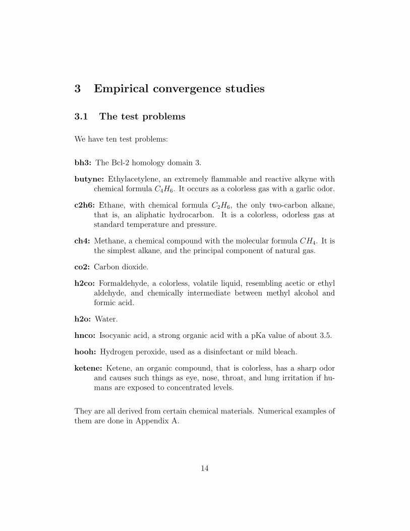
We have ten test problems:

bh3: The Bcl-2 homology domain 3.

butyne: Ethylacetylene, an extremely flammable and reactive alkyne withchemical formula C4H6. It occurs as a colorless gas with a garlic odor.

c2h6: Ethane, with chemical formula C2H6, the only two-carbon alkane,that is, an aliphatic hydrocarbon. It is a colorless, odorless gas atstandard temperature and pressure.

ch4: Methane, a chemical compound with the molecular formula CH4. It isthe simplest alkane, and the principal component of natural gas.

co2: Carbon dioxide.

h2co: Formaldehyde, a colorless, volatile liquid, resembling acetic or ethylaldehyde, and chemically intermediate between methyl alcohol andformic acid.

h2o: Water.

hnco: Isocyanic acid, a strong organic acid with a pKa value of about 3.5.

hooh: Hydrogen peroxide, used as a disinfectant or mild bleach.

ketene: Ketene, an organic compound, that is colorless, has a sharp odorand causes such things as eye, nose, throat, and lung irritation if hu-mans are exposed to concentrated levels.

They are all derived from certain chemical materials. Numerical examples ofthem are done in Appendix A.

14

3.2 Details of the SCF-Anderson implementations

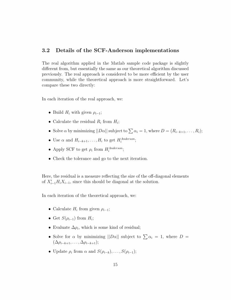
The real algorithm applied in the Matlab sample code package is slightlydifferent from, but essentially the same as our theoretical algorithm discussedpreviously. The real approach is considered to be more efficient by the usercommunity, while the theoretical approach is more straightforward. Let’scompare these two directly:

In each iteration of the real approach, we:

• Build Hi with given ρi−1;

• Calculate the residual Ri from Hi;

• Solve α by minimizing ||Dα|| subject to∑αi = 1, whereD = (Ri−k+1, . . . , Ri);

• Use α and Hi−k+1, . . . , Hi to get HAndersoni ;

• Apply SCF to get ρi from HAndersoni ;

• Check the tolerance and go to the next iteration.

Here, the residual is a measure reflecting the size of the off-diagonal elementsof X ′i−1HiXi−1, since this should be diagonal at the solution.

In each iteration of the theoretical approach, we:

• Calculate Hi from given ρi−1;

• Get S(ρi−1) from Hi;

• Evaluate ∆ρi, which is some kind of residual;

• Solve for α by minimizing ||Dα|| subject to∑αi = 1, where D =

(∆ρi−k+1, . . . ,∆ρi−k+1);

• Update ρi from α and S(ρi−k), . . . , S(ρi−1);

15

• Check the tolerance and go to the next iteration.

We can see that the real approach is mixing the Hamiltonian H, i.e., applyingthe Anderson Acceleration to H; while the theoretical approach is mixing thecharge density ρ. Now let’s look at the three critical steps in both approaches:

In the real approach:

• Mix H;

• Update ρ;

• Update H.

In the theoretical approach:

• Mix ρ;

• Update H;

• Update ρ.

Since H depends linearly on ρ, then mixing ρ and updating H would beequivalent to mixing H, and the two sets of algorithms would be identical.

Also, since ∆ρ is getting smaller in norm as the iteration converges, theD matrix may become more ill-conditioned if the columns from later itera-tionsare significantly smaller than those from earlier iterations. One possibleway to overcome this disadvantage is the strategy of dropping: to delete thefirst several columns of D as necessary, when ill conditioning occurs.

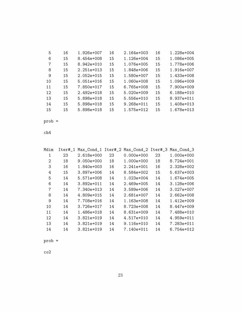
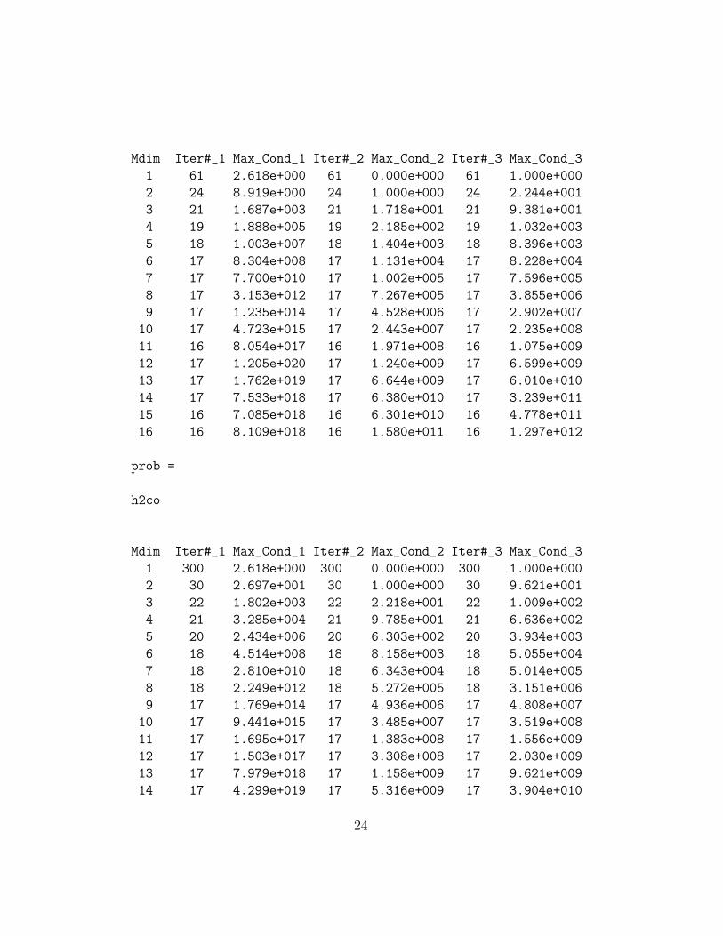
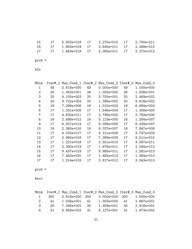
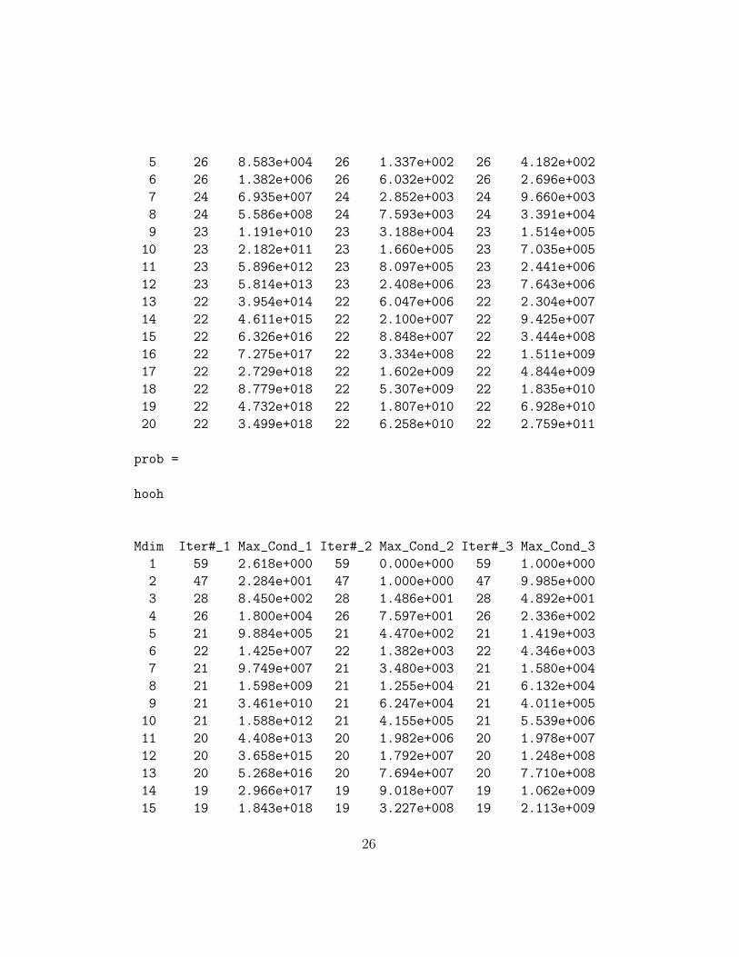
3.3 Effects of varying Mdim

There is one important variable in the Anderson Acceleration method, Mdim,which is the number of S(ρ)’s that are stored. There are four points relatingto this variable:

16

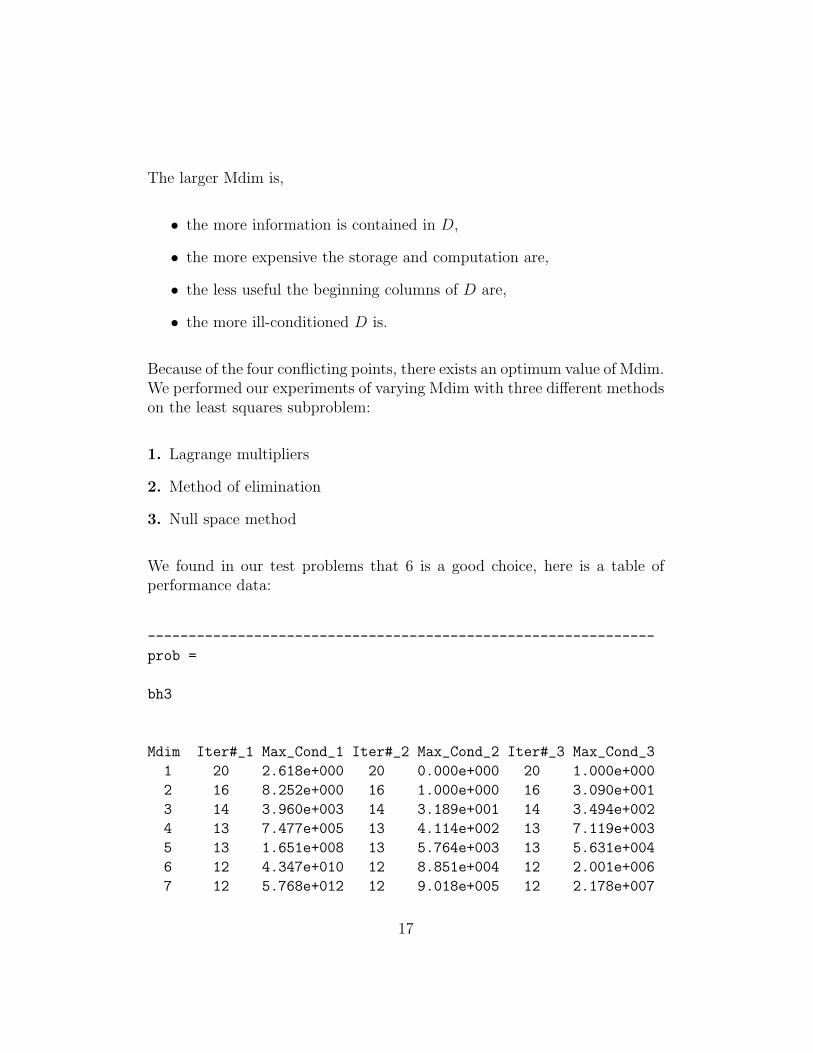
The larger Mdim is,

• the more information is contained in D,

• the more expensive the storage and computation are,

• the less useful the beginning columns of D are,

• the more ill-conditioned D is.

Because of the four conflicting points, there exists an optimum value of Mdim.We performed our experiments of varying Mdim with three different methodson the least squares subproblem:

1. Lagrange multipliers

2. Method of elimination

3. Null space method

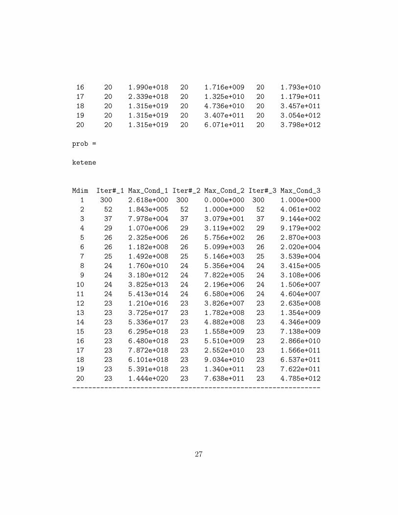
We found in our test problems that 6 is a good choice, here is a table ofperformance data:

--------------------------------------------------------------

prob =

bh3

Mdim Iter#_1 Max_Cond_1 Iter#_2 Max_Cond_2 Iter#_3 Max_Cond_3

1 20 2.618e+000 20 0.000e+000 20 1.000e+000

2 16 8.252e+000 16 1.000e+000 16 3.090e+001

3 14 3.960e+003 14 3.189e+001 14 3.494e+002

4 13 7.477e+005 13 4.114e+002 13 7.119e+003

5 13 1.651e+008 13 5.764e+003 13 5.631e+004

6 12 4.347e+010 12 8.851e+004 12 2.001e+006

7 12 5.768e+012 12 9.018e+005 12 2.178e+007

17

8 12 1.468e+015 12 1.523e+007 12 3.690e+008

9 12 4.550e+016 12 6.752e+007 12 1.739e+009

10 12 1.466e+019 12 1.116e+009 12 1.787e+010

11 12 9.221e+017 12 1.609e+010 12 3.334e+011

12 12 2.158e+018 12 3.262e+011 12 5.049e+012

--------------------------------------------------------------

Here, Iter# is the number of iterations before convergence; the upper limitis set to be 300. Max Cond is the maximum condition number of the linearsystems we solve.

We performed all the experiments without the strategy of dropping; completedata are in Appendix A.

3.4 Local and global convergence

In order to test the convergence properties of the SCF-Anderson method, ex-periments were performed in this way: We got an initial guess by perturbingthe solution (X∗) with random matrices,

X0 = X∗ + ε · randn(size(X∗)), (21)

where randn(n, k) is an n × k matrix with random entries normally dis-tributed, and size(X) with X ∈ Rn×k equals (n, k). If one of the initialguesses made from ε led to divergence, we reduce ε by half until we got con-vergence for 1000 trials with the same ε, and the last ε, which we denote byεr, will be the approximate radius of convergence.

Here is the experiment data:

Problem bh3 butyne c2h6 ch4 co2εr 1.0000e-04 6.2500e-06 2.5000e-05 2.5000e-05 5.0000e-05

Problem h2co h2o hnco hooh keteneεr 5.0000e-05 1.0000e-04 5.0000e-05 1.0000e-04 1.0000e-04

In these experiments, the SCF-Anderson method was locally convergent butnot globally convergent. Beyond the radius of convergence, as the perturba-tion gets bigger, convergence became less likely.

18

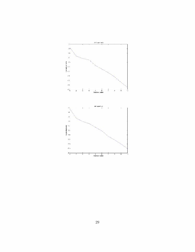
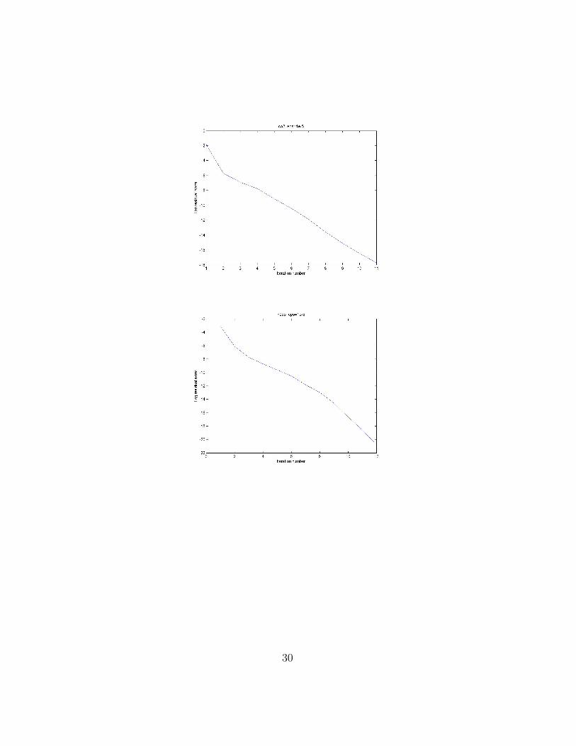
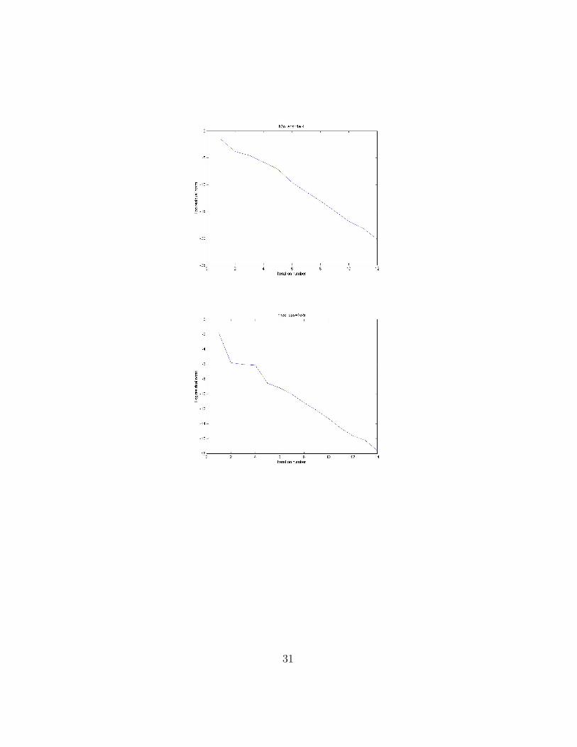
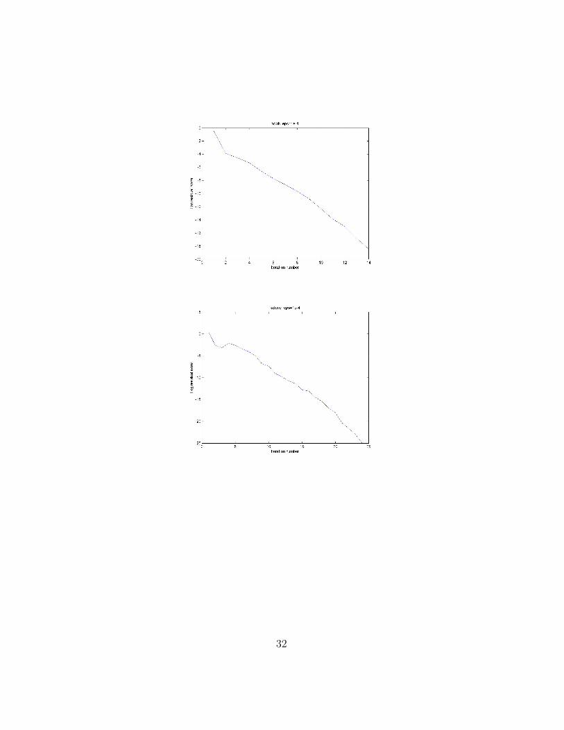
When the iterates converges, the convergence is linear, we use plots of itera-tion number versus log residual norm to illustrate this.

Here is an example of convergence under a “good” initial guess with ε = εr =1e− 4 for the bh3 problem:

Figure 1: Convergence

Note that the convergence is approximately linear, see Apprendix A2 foradditional examples.

Here is an example of divergence under a “bad” initial guess:

Figure 2: Divergence

19

4 Concluding summary

In this project, I:

• Learned the properties of SCF method and SCF-Anderson method,and found a new way to look at the problem.

• Studied several different approaches to the linearly constrained least-square subroutine.

• Studied the influence of the variable Mdim in the Anderson Accelera-tion method.

and I conclude that:

• For every Hamiltonian considered, there exists an optimal Mdim value.

• The Null-space method is better than the other three.

• The experiments suggest that the SCF-Anderson method could havelocal linear convergence.

For future work, I will:

• Find theoritical support for the Anderson Acceleration method, andimprove the performance from it.

• Apply the Anderson Acceleration method as an acceleration algorithmto general fixed point problems.

20

Appendix

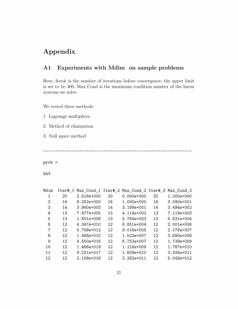
A1 Experiments with Mdim on sample problems

Here, Iter# is the number of iterations before convergence; the upper limitis set to be 300, Max Cond is the maximum condition number of the linearsystems we solve.

We tested three methods:

1. Lagrange multipliers

2. Method of elimination

3. Null space method

--------------------------------------------------------------

prob =

bh3


1 20 2.618e+000 20 0.000e+000 20 1.000e+000

2 16 8.252e+000 16 1.000e+000 16 3.090e+001

3 14 3.960e+003 14 3.189e+001 14 3.494e+002

4 13 7.477e+005 13 4.114e+002 13 7.119e+003

5 13 1.651e+008 13 5.764e+003 13 5.631e+004

6 12 4.347e+010 12 8.851e+004 12 2.001e+006

7 12 5.768e+012 12 9.018e+005 12 2.178e+007

8 12 1.468e+015 12 1.523e+007 12 3.690e+008

9 12 4.550e+016 12 6.752e+007 12 1.739e+009

10 12 1.466e+019 12 1.116e+009 12 1.787e+010

11 12 9.221e+017 12 1.609e+010 12 3.334e+011

12 12 2.158e+018 12 3.262e+011 12 5.049e+012

21

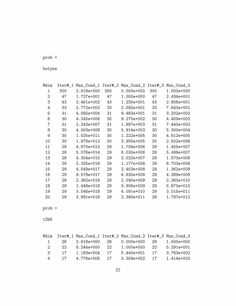
prob =

butyne


1 300 2.618e+000 300 0.000e+000 300 1.000e+000

2 47 1.727e+001 47 1.000e+000 47 2.434e+001

3 43 2.461e+002 43 1.230e+001 43 2.858e+001

4 33 2.772e+003 33 2.582e+001 33 7.643e+001

5 31 4.565e+004 31 9.483e+001 31 3.202e+002

6 30 4.245e+006 30 9.275e+002 30 4.459e+003

7 31 2.243e+007 31 1.887e+003 31 7.443e+003

8 30 4.003e+008 30 5.914e+003 30 5.300e+004

9 30 1.025e+011 30 1.222e+005 30 4.612e+005

10 30 1.878e+012 30 3.955e+005 30 2.502e+006

11 29 4.670e+013 29 1.706e+006 29 1.455e+007

12 29 5.076e+014 29 6.030e+006 29 5.499e+007

13 29 4.304e+015 29 2.022e+007 29 1.573e+008

14 29 2.325e+018 29 1.177e+008 29 8.703e+008

15 29 4.549e+017 29 2.453e+008 29 1.362e+009

16 29 9.578e+017 29 6.630e+008 29 4.389e+009

17 29 2.382e+018 29 2.590e+009 29 2.363e+010

18 29 1.448e+018 29 9.906e+009 29 5.870e+010

19 29 3.546e+018 29 4.091e+010 29 3.015e+011

20 29 3.891e+018 29 2.390e+011 29 1.797e+012

prob =

c2h6


1 28 2.618e+000 28 0.000e+000 28 1.000e+000

2 22 8.244e+000 22 1.000e+000 22 5.291e+001

3 17 1.183e+004 17 5.440e+001 17 3.763e+002

4 17 4.776e+005 17 3.309e+002 17 1.414e+003

22

5 16 1.926e+007 16 2.164e+003 16 1.228e+004

6 15 8.454e+008 15 1.126e+004 15 1.086e+005

7 15 8.942e+010 15 1.076e+005 15 1.778e+006

8 15 2.251e+013 15 1.848e+006 15 1.916e+007

9 15 2.052e+015 15 1.580e+007 15 1.433e+008

10 15 5.051e+016 15 1.060e+008 15 1.096e+009

11 15 7.850e+017 15 6.765e+008 15 7.900e+009

12 15 2.492e+018 15 5.020e+009 15 6.188e+010

13 15 5.898e+018 15 5.556e+010 15 8.937e+011

14 15 5.898e+018 15 9.268e+011 15 1.408e+013

15 15 5.898e+018 15 1.575e+012 15 1.678e+013

prob =

ch4


1 23 2.618e+000 23 0.000e+000 23 1.000e+000

2 18 9.050e+000 18 1.000e+000 18 8.724e+001

3 16 1.840e+003 16 2.241e+001 16 2.328e+002

4 15 3.897e+006 14 8.584e+002 15 5.637e+003

5 14 5.571e+008 14 1.023e+004 14 1.674e+005

6 14 3.892e+011 14 2.469e+005 14 3.128e+006

7 14 7.340e+013 14 3.589e+006 14 3.027e+007

8 14 4.809e+015 14 2.681e+007 14 2.662e+008

9 14 7.708e+016 14 1.163e+008 14 1.412e+009

10 14 3.726e+017 14 8.723e+008 14 8.447e+009

11 14 1.486e+018 14 8.631e+009 14 7.488e+010

12 14 3.821e+019 14 4.517e+010 14 4.959e+011

13 14 3.821e+019 14 9.116e+010 14 7.283e+011

14 14 3.821e+019 14 7.140e+011 14 6.754e+012

prob =

co2

23


1 61 2.618e+000 61 0.000e+000 61 1.000e+000

2 24 8.919e+000 24 1.000e+000 24 2.244e+001

3 21 1.687e+003 21 1.718e+001 21 9.381e+001

4 19 1.888e+005 19 2.185e+002 19 1.032e+003

5 18 1.003e+007 18 1.404e+003 18 8.396e+003

6 17 8.304e+008 17 1.131e+004 17 8.228e+004

7 17 7.700e+010 17 1.002e+005 17 7.596e+005

8 17 3.153e+012 17 7.267e+005 17 3.855e+006

9 17 1.235e+014 17 4.528e+006 17 2.902e+007

10 17 4.723e+015 17 2.443e+007 17 2.235e+008

11 16 8.054e+017 16 1.971e+008 16 1.075e+009

12 17 1.205e+020 17 1.240e+009 17 6.599e+009

13 17 1.762e+019 17 6.644e+009 17 6.010e+010

14 17 7.533e+018 17 6.380e+010 17 3.239e+011

15 16 7.085e+018 16 6.301e+010 16 4.778e+011

16 16 8.109e+018 16 1.580e+011 16 1.297e+012

prob =

h2co


1 300 2.618e+000 300 0.000e+000 300 1.000e+000

2 30 2.697e+001 30 1.000e+000 30 9.621e+001

3 22 1.802e+003 22 2.218e+001 22 1.009e+002

4 21 3.285e+004 21 9.785e+001 21 6.636e+002

5 20 2.434e+006 20 6.303e+002 20 3.934e+003

6 18 4.514e+008 18 8.158e+003 18 5.055e+004

7 18 2.810e+010 18 6.343e+004 18 5.014e+005

8 18 2.249e+012 18 5.272e+005 18 3.151e+006

9 17 1.769e+014 17 4.936e+006 17 4.808e+007

10 17 9.441e+015 17 3.485e+007 17 3.519e+008

11 17 1.695e+017 17 1.383e+008 17 1.556e+009

12 17 1.503e+017 17 3.308e+008 17 2.030e+009

13 17 7.979e+018 17 1.158e+009 17 9.621e+009

14 17 4.299e+019 17 5.316e+009 17 3.904e+010

24

15 17 5.932e+018 17 2.275e+010 17 2.740e+011

16 17 1.663e+019 17 2.645e+011 17 2.268e+012

17 17 1.663e+019 17 4.065e+011 17 2.270e+012

prob =

h2o


1 49 2.618e+000 49 0.000e+000 49 1.000e+000

2 26 1.062e+001 26 1.000e+000 26 1.838e+001

3 20 4.105e+003 20 3.750e+001 20 2.469e+002

4 20 9.722e+004 20 1.386e+002 20 9.818e+002

5 18 7.298e+006 18 1.015e+003 18 6.684e+003

6 17 1.331e+009 17 1.546e+004 17 1.356e+005

7 17 4.830e+011 17 2.796e+005 17 2.783e+006

8 16 2.688e+012 16 5.123e+005 16 1.264e+007

9 17 6.057e+014 17 8.096e+006 17 8.439e+007

10 16 2.390e+016 16 6.027e+007 16 7.847e+008

11 17 4.032e+017 17 9.211e+008 17 9.747e+009

12 17 2.990e+018 17 7.369e+009 17 9.511e+010

13 17 1.221e+018 17 2.551e+010 17 4.267e+011

14 17 2.290e+019 17 1.878e+011 17 2.044e+012

15 17 9.437e+019 17 8.985e+011 17 1.281e+013

16 17 7.450e+020 17 1.465e+012 17 1.383e+013

17 17 1.214e+018 17 2.817e+012 17 3.543e+013

prob =

hnco


1 300 2.618e+000 300 0.000e+000 300 1.000e+000

2 41 1.539e+001 41 1.000e+000 41 2.667e+001

3 35 7.285e+002 35 1.359e+001 35 3.918e+001

4 31 9.958e+003 31 6.137e+001 31 1.973e+002

25

5 26 8.583e+004 26 1.337e+002 26 4.182e+002

6 26 1.382e+006 26 6.032e+002 26 2.696e+003

7 24 6.935e+007 24 2.852e+003 24 9.660e+003

8 24 5.586e+008 24 7.593e+003 24 3.391e+004

9 23 1.191e+010 23 3.188e+004 23 1.514e+005

10 23 2.182e+011 23 1.660e+005 23 7.035e+005

11 23 5.896e+012 23 8.097e+005 23 2.441e+006

12 23 5.814e+013 23 2.408e+006 23 7.643e+006

13 22 3.954e+014 22 6.047e+006 22 2.304e+007

14 22 4.611e+015 22 2.100e+007 22 9.425e+007

15 22 6.326e+016 22 8.848e+007 22 3.444e+008

16 22 7.275e+017 22 3.334e+008 22 1.511e+009

17 22 2.729e+018 22 1.602e+009 22 4.844e+009

18 22 8.779e+018 22 5.307e+009 22 1.835e+010

19 22 4.732e+018 22 1.807e+010 22 6.928e+010

20 22 3.499e+018 22 6.258e+010 22 2.759e+011

prob =

hooh


1 59 2.618e+000 59 0.000e+000 59 1.000e+000

2 47 2.284e+001 47 1.000e+000 47 9.985e+000

3 28 8.450e+002 28 1.486e+001 28 4.892e+001

4 26 1.800e+004 26 7.597e+001 26 2.336e+002

5 21 9.884e+005 21 4.470e+002 21 1.419e+003

6 22 1.425e+007 22 1.382e+003 22 4.346e+003

7 21 9.749e+007 21 3.480e+003 21 1.580e+004

8 21 1.598e+009 21 1.255e+004 21 6.132e+004

9 21 3.461e+010 21 6.247e+004 21 4.011e+005

10 21 1.588e+012 21 4.155e+005 21 5.539e+006

11 20 4.408e+013 20 1.982e+006 20 1.978e+007

12 20 3.658e+015 20 1.792e+007 20 1.248e+008

13 20 5.268e+016 20 7.694e+007 20 7.710e+008

14 19 2.966e+017 19 9.018e+007 19 1.062e+009

15 19 1.843e+018 19 3.227e+008 19 2.113e+009

26

16 20 1.990e+018 20 1.716e+009 20 1.793e+010

17 20 2.339e+018 20 1.325e+010 20 1.179e+011

18 20 1.315e+019 20 4.736e+010 20 3.457e+011

19 20 1.315e+019 20 3.407e+011 20 3.054e+012

20 20 1.315e+019 20 6.071e+011 20 3.798e+012

prob =

ketene


1 300 2.618e+000 300 0.000e+000 300 1.000e+000

2 52 1.843e+005 52 1.000e+000 52 4.061e+002

3 37 7.978e+004 37 3.079e+001 37 9.144e+002

4 29 1.070e+006 29 3.119e+002 29 9.179e+002

5 26 2.325e+006 26 5.756e+002 26 2.870e+003

6 26 1.182e+008 26 5.099e+003 26 2.020e+004

7 25 1.492e+008 25 5.146e+003 25 3.539e+004

8 24 1.760e+010 24 5.356e+004 24 3.415e+005

9 24 3.180e+012 24 7.822e+005 24 3.108e+006

10 24 3.825e+013 24 2.196e+006 24 1.506e+007

11 24 5.413e+014 24 6.580e+006 24 4.604e+007

12 23 1.210e+016 23 3.826e+007 23 2.635e+008

13 23 3.725e+017 23 1.782e+008 23 1.354e+009

14 23 5.336e+017 23 4.882e+008 23 4.346e+009

15 23 6.295e+018 23 1.558e+009 23 7.138e+009

16 23 6.480e+018 23 5.510e+009 23 2.866e+010

17 23 7.872e+018 23 2.552e+010 23 1.566e+011

18 23 6.101e+018 23 9.034e+010 23 6.537e+011

19 23 5.391e+018 23 1.340e+011 23 7.622e+011

20 23 1.444e+020 23 7.638e+011 23 4.785e+012

--------------------------------------------------------------

27

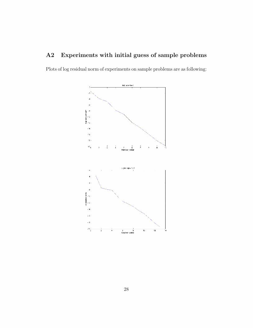
A2 Experiments with initial guess of sample problems

Plots of log residual norm of experiments on sample problems are as following:

28

References

[1] D. G. Anderson. Iterative procedures for nonlinear integral equations. J.Assoc. Comput. Mach., 12:547–560, 1965.

[2] Ake Bjorck. Numerical methods for least squares problems. Society forIndustrial and Applied Mathematics (SIAM), Philadelphia, PA, 1996.

[3] Claude Le Bris. Computational chemistry from the perspective of nu-merical analysis. Acta Numerica, 14:363–444, 2005.

[4] Gene H. Golub and Charles F. Van Loan. Matrix computations. JohnsHopkins Studies in the Mathematical Sciences. Johns Hopkins UniversityPress, Baltimore, MD, third edition, 1996.

[5] Georg Kresse and Jurgen Furthmuller. Efficiency of ab-initio total energycalculations for metals and semiconductors using a plane-wave basis set.Computational Materials Science, 6:15–50, 1996.

[6] Peter Pulay. Convergence acceleration of iterative sequences. the case ofscf iteration. Chem. Phys. Letters, 73(2):393–398, 1980.

[7] Chao Yang, Juan C. Meza, and Lin-Wang Wang. A trust region directconstrained minimization algorithm for the Kohn-Sham equation. SIAMJ. Sci. Comput., 29(5):1854–1875 (electronic), 2007.

33

the scf-anderson method for a non-linear eigenvalue problem

Documents