the safety analysis concept of welded components … d… · the safety analysis concept of welded...
TRANSCRIPT
THE SAFETY ANALYSIS CONCEPT OF WELDED
COMPONENTS UNDER CYCLIC LOADS USING
FRACTURE MECHANICS METHOD
Von der Fakultät für Werkstoffwissenschaft und Werkstofftechnologie
der Technischen Universität Bergakademie Freiberg
genehmigte
DISSERTATION
zur Erlangung des akademischen Grades
Doktor-Ingenieur
Dr.-Ing.
vorgelegt
von M.Sc. Ahmed M. Al-Mukhtar geboren am 10. November 1976 in Bagdad, Irak
Gutachter: Prof. Dr.-Ing. habil. Horst Biermann, Freiberg
Prof. Dr.-Ing. Peter Hübner, Mittweida
Prof. Dr.-Ing. Uwe Zerbst, Berlin
Tag der Verleihung: 16.06.2010
Institute of Materials Engineering Faculty of Materials Science and Technology Technische Universität Bergakademie Freiberg, Germa ny
THE SAFETY ANALYSIS CONCEPT OF WELDED
COMPONENTS UNDER CYCLIC LOADS USING
FRACTURE MECHANICS METHOD
By
M.Sc. Ahmed M. Al-Mukhtar
Approved by:
Prof. Dr.-Ing. habil. Horst Biermann Faculty of Materials Science and Technology Institute of Materials Engineering TUB Freiberg
Prof. Dr.-Ing. Peter Hübner Faculty of Mechanical Engineering University of Applied Science, Mittweida
Prof. Dr.-Ing. Uwe Zerbst Federal Institute for Materials Research and Testin g BAM, Berlin
Prof. Dr.-Ing. Lutz Krüger Faculty of Materials Science and Technology Institute of Materials Engineering TUB Freiberg
Prof. Dr.-Ing. Matthias Kröger Institute for Machine Elements, Design and Manufacturing Faculty of Mechanical, Process and Energy Engineering, TUB Freiberg
Prof. Dr.-Ing. Klaus Eigenfeld Faculty of Materials Science and Technology Foundry Institute, TUB Freiberg
Date of Approved: 16.06.2010

To the people who are always by my side,
My wonderful mother, my wife and my children
I
ACKNOWLEDGEMENTS
I would like to acknowledge the Free State of Saxony “Freistaates Sachsen” for the
award of scholarship that enabled me to undertake this research work at Technische
Universität Bergakademie Freiberg, Institute of Materials Engineering, Germany.
My special thanks go to my supervisor, Prof. Dr.-Ing. habil. H. Biermann, Head of
the Institute of Materials Engineering for the support, encouragement and provide me
the supportive things to my life and study during the period of my research.
Also, I would like to thank my supervisor, Prof. Dr.-Ing. P. Hübner, Faculty of
Mechanical Engineering, University of Applied Science, Mittweida.
Thanks also to Prof. Dr.-Ing. Uwe Zerbst from Federal Institute for Materials
Research and Testing (BAM) for many fruitful discussions and comments.
My thanks go to my colleague Dipl.-Ing. S. Henkel, Institute of Materials
Engineering, for his guidance, technical support and helpful discussions during the
course of this research.
I have to remember with warm affection and thanks, the sympathetic woman Mrs.
Edda Paul, for her kind help during my study application through the frame of PhD
program (TUBA Freiberg). Also I have to thank the coordinator of PhD program, Dr.
Corina Dunger for supporting.
I have to thank Prof. Dr. M. Mirzaei, Department of Mechanical Engineering, TM
University, for his help and benefit discussions during the time of this work.
I would also like to thank all my fellow graduate students in Institute of Materials
Engineering, for their kind response with my all requests. In particular, I’m grateful to,
Gundis Sacher, Marco Klemm, Tomas Mottitschka and Kai Nagel for their help and
fellowship. All members in Institute of Materials Engineering are gratefully
acknowledged. Thanks for Dr.-Ing. Abdulkader Kadauw, Institute of Mechanical
Engineering, and Dr.-Ing. A. Al-Zoubi, Institute of Thermal Engineering (TUBA
Freiberg).
Thanks for Dr. Ebtihal Abas, College of Engineering, University of Baghdad, for her
kind responses with my requests. My thanks also for Mr. Ahmed Qadoury Abed, Al-
Mustansiriyah University, College of Arts, Department of Translation for his help.
Finally, I would like to express my profound gratitude to my family, especially my
mother, for their support and encouragement throughout my education and professional
career and for putting up with me the past few years. To my father, Mr. Majeed Al-

II
Mukhtar, and father in law Mr. Abdulelah Jwair in grateful memory. My thanks go to
my wife Rawa Abdul Elah Jwair, who has sacrificed time to complete this work. To my
daughters Dania and Bainat, who makes my life worth I dedicate this work.
III
ABSTRACT
Fracture Mechanics process of Welded Joint is a very vast research area and has
many possibilities for solution and prediction. Although the fatigue strength (FAT) and
stress intensity factor (SIF) solutions are reported in several handbooks and
recommendations, these values are available only for a small number of specimens,
components, loading and welding geometries. The available solutions are not always
adequate for particular engineering applications. Moreover, the reliable solutions of SIF
are still difficult to find in spite of several SIF handbooks have been published
regarding the nominal applied SIF. The effect of residual stresses is still the most
challenge in fatigue life estimation. The reason is that the stress distributions and SIF
modified by the residual stresses have to be estimated. The stress distribution is
governed by many parameters such as the materials type, joint geometry and welding
processes.
In this work, the linear elastic fracture mechanics (LEFM), which used crack tip SIFs
for cases involving the effect of weld geometry, is used to calculate the crack growth
life for some different notch cases.
The variety of crack configurations and the complexity of stress fields occurring in
engineering components require more versatile tools for calculating SIFs than available
in handbook’s solutions that were obtained for a range of specific geometries and load
combinations.
Therefore, the finite element method (FEM) has been used to calculate SIFs of
cracks subjected to stress fields. LEFM is encoded in the FEM software, FRANC,
which stands for fracture analysis code.
The SIFs due to residual stress are calculated in this work using the weight function
method.
The fatigue strength (FAT) of load-carrying and non-load carrying welded joints
with lack of penetration (LOP) and toe crack, respectively, are determined using the
LEFM. In some studied cases, the geometry, material properties and loading conditions
of the joints are identical to those of specimens for which experimental results of fatigue
life and SIF were available in literature so that the FEM model could be validated.
For a given welded material and set of test conditions, the crack growth behavior is
described by the relationship between cyclic crack growth rate, da/dN, and range of the
stress intensity factor (∆K) , i.e., by Paris’ law. Numerical integration of the Paris’
IV
equation is carried out by a FORTRAN computer routine. The obtained results can be
used for calculating FAT values. The computed SIFs along with the Paris’ law are used
to predict the crack propagation. The typical crack lengths for each joint geometry are
determined using the built language program by backward calculations.
To incorporate the effect of residual stresses, the fatigue crack growth equations
which are sensitive to stress ratio R are recommended to be used. The Forman, Newman
and de Konig (FNK) solution is considered to be the most suitable one for the present
purpose.
In spite of the recent considerable progress in fracture mechanics theories and
applications, there seems to be no, at least to the author’s knowledge, systematic study
of the effect of welding geometries and residual stresses upon fatigue crack propagation
based completely on an analytical approach where the SIF due to external applied load
(Kapp) is calculated using FEM. In contrast, the SIF due to residual stresses (Kres) is
calculated using the analytical weight function method and residual stress distribution.
To assess the influence of the residual stresses on the failure of a weldment, their
distribution must be known.
Although residual stresses in welded structures and components have long been
known to have an effect on the components fatigue performance, access to reliable,
spatially accurate residual stress field data are limited. This work constitutes a
systematic research program regarding the concept for the safety analysis of welded
components with fracture mechanics methods, to clarify the effect of welding residual
stresses upon fatigue crack propagation.
V
KURZREFERAT
Al-Mukhtar, Ahmed Doktorarbeit, Technische Universität Bergakademie F reiberg Fakultät für Werkstoffwissenschaft und Werkstofftec hnologie Institut für Werkstofftechnik
Die Bewertung einer Schweißnaht ist ein großes Forschungsgebiet und hat viele
Möglichkeiten für Lösungskonzepte und Vorhersagen. Obwohl für die
Schwingfestigkeit und die Spannungsintensitätsfaktor (SIF)-Lösungen in verschiedenen
Handbüchern Empfehlungen ausgewiesen sind, sind diese Werte nur für eine geringe
Anzahl von Proben, Komponenten, Belastungsfälle und Schweißgeometrien verfügbar.
Die vorhandenen Lösungsansätze sind nicht immer für spezielle technische
Anwendungen geeignet. Darüber hinaus sind zuverlässige bewährte Lösungen von
Spannungsintensitätsfaktoren immer noch schwierig zu finden, obwohl verschiedene
SIF-Handbücher mit Hinweis auf den anliegenden nominalen SIF veröffentlicht sind.
Der Einfluss von Eigenspannungen ist eine der größten Herausforderungen bei der
Lebensdauerabschätzung. Aufgrund der Tatsache, dass infolge der Eigenspannungen
sowohl die Spannungsverteilung als auch der SIF verändert werden, muss eine
Abschätzung erfolgen. Die Spannungsverteilung wird durch viele Parameter beeinflusst,
wie zum Beispiel den Werkstoff, die Nahtgeometrie und den Schweißprozess.
In der vorliegenden Arbeit wurde für die Berechnung des Ermüdungsrisswachstums
unter verschiedenen Kerbfällen das Konzept der linear-elastischen Bruchmechanik
(LEBM) verwendet, welches K-Lösungen für die Rissspitze bei unterschiedlichen
Fällen der Schweißgeometrie berücksichtigt.
Aufgrund der Komplexität der Risskonfigurationen und der Spannungsfelder in
praxisrelevanten Komponenten werden weitere Hilfsmittel zur Berechnung von
Spannungsintensitätsfaktoren benötigt, welche die herkömmlichen Lösungen in
Handbüchern erweitern.
Deshalb wurde die Finite Elemente Methode (FEM) zur Berechnung von
Spannungsintensitätsfaktoren an Rissen verwendet. Die LEBM wird in der FEM-
Software FRANC berücksichtigt.
Die aus Eigenspannungen resultierenden Spannungsintensitätsfaktoren wurden mit
Hilfe der Gewichtsfunktionsmethode berechnet.
VI
Die Ermüdungslebensdauer (Schwingfestigkeit) von tragenden und nichttragenden
Schweißnähten mit ungenügender Durchschweißung beziehungsweise Kerbriss wurden
mit Hilfe der LEBM durch Integration der Zyklischen Risswachstumskurve ermittelt.
Zur Validierung des FEM-Modells konnte in einigen untersuchten Fällen auf
experimentelle Ergebnisse zur Lebensdauer und zum SIF aus der Literatur
zurückgegriffen werden, wo identische Geometrien, Materialeigenschaften und
Belastungsverhältnisse der Naht vorlagen.
Unter Vorgabe des Werkstoffes und der Prüfbedingungen wurde das
Risswachstumsverhalten mit dem Zusammenhang von Risswachstumsgeschwindigkeit
da/dN und zyklischem Spannungsintensitätsfaktor ∆K mit dem Paris-Gesetz
beschrieben. Eine numerische Integration der Paris-Gleichung erfolgte über ein
FORTRAN-Programm. Die damit erhaltenen Ergebnisse sind als
Ermüdungslebensdauer (Schwingfestigkeit) verwendbar. Die berechneten SIF‘en
entlang der Paris-Geraden werden zur Vorhersage des Risswachstums benutzt. Die
typischen Risslängen für jede Nahtgeometrie wurden mit Hilfe des eigens integrierten
Programmes ermittelt.
Zur Berücksichtigung des Einflusses von Eigenspannungen wird empfohlen,
Risswachstumsgleichungen zu nutzen, die empfindlich auf das Spannungsverhältnis R
reagieren. Für die vorliegende Zielsetzung gilt der Lösungsansatz nach Forman,
Newman und de Konig (FNK) als der am besten geeignete.
Trotz der jüngsten, beträchtlichen Fortschritte in den bruchmechanischen Theorien
und Anwendungen sind systematische Studien zum Einfluss der Schweißgeometrie und
der Eigenspannungen auf das Ermüdungsrisswachstum, in welchen der SIF aufgrund
extern anliegender Beanspruchungen (Kapp) mit der FEM berechnet wurde, in der
Literatur kaum vorhanden. Im Gegensatz dazu wurde der SIF infolge von
Eigenspannungen (Kres) mit Hilfe der analytischen Gewichtsfunktionsmethode und der
Eigenspannungsverteilung berechnet. Um den Einfluss von Eigenspannungen auf das
Versagen einer Schweißverbindung abzuschätzen, muss deren Verteilung bekannt sein.
Obwohl die Wirkung von Eigenspannungen auf das Ermüdungsverhalten in
geschweißten Strukturen und Komponenten schon lange bekannt ist, ist der Zugriff auf
verlässliche und präzise Daten von räumlichen Eigenspannungsfeldern begrenzt.
Bezüglich einer konzeptionellen Sicherheitsanalyse von geschweißten Komponenten
mit bruchmechanischen Methoden begründet diese Arbeit einen systematischen Ansatz,
VII
um den Einfluss von Schweißeigenspannungen auf das Ermüdungsrisswachstum zu
verdeutlichen.

VIII
LIST OF PUBLICATIONS FROM THIS RESEACH
A. Published or Accepted
1. Al-Mukhtar A., Biermann H., Hübner P. and Henkel S., Lebensdauerberechnung
von Schweissverbindungen mit bruchmechanischen Meth oden (Fatigue Life
Calculation of Welded Joints with Fracture Mechanic s Methods) , 41 Tagung des DVM-
Arbeitskreises Bruchvorgänge, Wuppertal, Germany, pp. 63–72, February 17–18, 2009, (In
German).
2. Al-Mukhtar A., Biermann H., Hübner P. and Henkel S., Fatigue Life Prediction of
Fillet Welded Cruciform Joints Based on Fracture Me chanics Method , Proceedings of
2nd International Conference on Fatigue and Fracture in the Infrastructure, Philadelphia,
USA, July 26–29, 2009.
3. Al-Mukhtar A., Biermann H., Hübner P. and Henkel S., Fatigue Crack Propagation
Life Calculation in Welded Joints , CD of International Conference on Crack Paths (CP
2009), Italy, pp. 391–397, September 23–25, 2009.
4. Al-Mukhtar A., Biermann H., Hübner P. and Henkel S., A Finite Element Calculation
of Stress Intensity Factors of Cruciform and Butt W elded Joints for Some
Geometrical Parameters , Jordan J. Mech. Indus. Eng. (JJMIE), Vol. 3, No. 4, pp. 236–245,
2009. ISSN 1995-6665.
5. Al-Mukhtar A., Biermann H., Hübner P. and Henkel S., Comparison of the Stress
Intensity Factor of Load-Carrying Cruciform Welded Joints with Different Geometries ,
Journal of Materials Engineering and Performance (JMEP), ASM International, (Accepted
for publication), 2010. Doi: 10.1007/s11665-009-9552-1.
6. Al-Mukhtar A., Biermann H., Hübner P. and Henkel S., Determination of Some
Parameters for Fatigue Life in Welded Joints Using Fracture Mechanics Method ,
Journal of Materials Engineering and Performance (JMEP), ASM International, (Accepted
for publication), 2010. Doi: 10.1007/s11665-010-9621-5.
B. Submitted and under Review Process
7. Al-Mukhtar A., Biermann H., Hübner P. and Henkel S.,The Effect of Weld Profile and
Geometries of Butt Weld Joints on Fatigue Life Unde r Cyclic Tensile Loading , Journal
of Materials Engineering and Performance (JMEP), ASM International, (In review).
IX
TABLE OF CONTENTS
ACKNOWLEDGEMENTS................................... .........................................................I ABSTRACT........................................... .....................................................................III KURZREFERAT ........................................ ................................................................ V LIST OF PUBLICATIONS FROM THIS RESEACH............. ................................... VIII TABLE OF CONTENTS.................................. .......................................................... IX NOMENCLATURE AND ABBREVIATIONS..................... ....................................... XII Chapter One INTRODUCTION.........................................................................................................1
1.1. Background and Motivation of the Research ....................................................1 1.2. Fatigue Failure..................................................................................................2 1.3. Failure of Welded Joints ...................................................................................5 1.3.1. Butt Welded Joints .........................................................................................6 1.3.2. Cruciform Fillet Welded Joints .......................................................................7 1.3.2.1. Non-Load Carrying Fillet Weld....................................................................8 1.3.2.2. Load-Carrying Fillet Weld ...........................................................................8 1.4. Concept of Fracture Mechanics Methods .........................................................9 1.5. Residual Stresses in Welding .........................................................................10 1.6. Objectives and Scope.....................................................................................11 1.7. Outline of the Thesis .......................................................................................12 1.8. The Present Work...........................................................................................13
Chapter Two LITERATURE REVIEW.................................. ...........................................................15
2.1. Introduction .....................................................................................................15 2.2. Fracture Mechanics of Fillet Welded Joints ....................................................15 2.3. Crack Propagation Curve................................................................................22 2.4. Simulation of Fatigue Crack Growth ...............................................................25 2.5. Fracture Analysis Code...................................................................................27 2.6. Factors Affecting the Fatigue Strength of Welded Joints ................................28 2.6.1. Weld Geometry............................................................................................29 2.6.2. Weld Defects and Metallurgy .......................................................................36 2.6.3. Materials and Welding Techniques..............................................................37 2.6.4. Weld Residual Stresses...............................................................................37 2.7. Residual Stress Effects on Fatigue Life of Welded Joints...............................38 2.7.1. Crack Closure and Effective SIF..................................................................40 2.7.2. Determination of Residual Stresses.............................................................42 2.8. Superposition Method.....................................................................................45 2.8.1. Residual Stresses Distribution .....................................................................46 2.8.1.1. R6 Distributions for T-Plate.......................................................................47 2.8.1.2. Polynomial Distributions for T-Plate and Butt Welds.................................47 2.8.2. Residual Stress Intensity Factor ..................................................................48 2.9. Conclusions and Discussion of Current Work.................................................54
Chapter Three MODELING OF WELDED JOINTS AND SIF CALCULATION...... ...........................58
3.1. Introduction .....................................................................................................58

X
3.2. Two Dimensional Analysis of Welded Joints...................................................59 3.3. Finite Element Analysis...................................................................................61 3.4. Mesh Description and Boundary Conditions ...................................................61 3.5. Material Properties..........................................................................................63 3.6. Solution Procedure .........................................................................................64 3.6.1. Mesh Generation .........................................................................................65 3.6.2. Selection of Material Model..........................................................................65 3.6.3. Crack Propagation .......................................................................................66 3.6.4. Modeling Procedures...................................................................................66 3.7. Results Convergence......................................................................................68 3.7.1. Influence of Mesh Size.................................................................................69 3.7.2. Influence of Crack Increment .......................................................................71 3.7.3. Influence of Mesh Type................................................................................73 3.7.4. Influence of Symmetry .................................................................................75 3.8. Selection of the Notch Cases..........................................................................77 3.9. Stress Intensity Factor Calculations................................................................78 3.9.1. SIF of Load-Carrying Cruciform Joints.........................................................79 3.9.2. SIF of Non-Load-Carrying Cruciform Joints .................................................82 3.9.3. SIF of Transverse Butt Weld Joints having Toe Crack.................................84 3.9.4. SIF of Transverse Butt Weld joints having LOP...........................................85 3.10. Results and Discussion.................................................................................86 3.10.1. Cruciform Fillet Weld Model.......................................................................86 3.10.2. Stress Distribution......................................................................................86 3.10.3. Butt Weld Model.........................................................................................90 3.10.4. Results of Verifications ..............................................................................91 3.10.4.1. SIF of Non-Load-Carrying Cruciform Joints ............................................91 3.10.4.2. SIF of Load-Carrying Cruciform Joints....................................................93 3.10.4.3. SIF of Transverse Butt Weld Joints having Toe Crack............................94 3.10.4.4. SIF of Transverse Butt Weld Joints having LOP.....................................95 3.11. Effect of Geometry in Load-Carrying Cruciform Joints..................................96 3.11.1. Effect of Weld Shape .................................................................................96 3.11.2. Effect of Plate Thickness Ratio ..................................................................98 3.12. Conclusions ..................................................................................................99
Chapter Four FATIGUE LIFE CALCULATIONS AND VERIFICATIONS ........ .............................101
4.1. Introduction ...................................................................................................101 4.2. Fracture Mechanics Analysis ........................................................................103 4.3. Fatigue Life Calculations Using Paris’ Law...................................................104 4.4. Fatigue Life Calculation Using NASGRO Equation.......................................107 4.5. Parameters of Crack Propagation Life..........................................................109 4.6. Selection of the Notch Cases........................................................................110 4.7. Backward Calculation of Fatigue Strength ....................................................111 4.8. Results and Discussion.................................................................................114 4.8.1. Fatigue life Calculations.............................................................................114 4.8.1.1. Cruciform Weld Joints having Toe Crack................................................115 4.8.1.2. Transverse Butt Weld Joints having Toe Crack ......................................119 4.8.1.3. Cruciform Weld Joints having LOP .........................................................120 4.8.1.4. Transverse Butt Weld Joints having LOP ...............................................123 4.9. Experimental Verifications ............................................................................127
XI
4.10. Effect of Residual Stresses.........................................................................135 4.11. Effect of Sheet Thickness ...........................................................................135 4.12. Geometrical Verification of Butt Weld Joints ...............................................143 4.12.1. Simulation of Fatigue Crack Growth ........................................................143 4.12.2. Failure Mode............................................................................................145 4.12.3. Weld Metallurgy and Defects ...................................................................145 4.12.4. Fatigue Life and Crack Growth ................................................................147 4.12.5. Modeling ..................................................................................................148 4.12.6. Verification Results ..................................................................................148 4.12.7. Standards Verifications ............................................................................153 4.13. Conclusions ................................................................................................155
Chapter Five RESIDUAL STRESSES IN WELDED JOINTS................. ......................................157
5.1. Introduction ...................................................................................................157 5.2. Assumptions in Finite Element Model...........................................................158 5.3. Residual Stresses Assessment ....................................................................159 5.4. Residual Stress Intensity Factor ...................................................................161 5.5. Residual Stresses Distribution ......................................................................164 5.6. BSI 7910 Distribution ....................................................................................166 5.7. Total Stress Intensity Factor .........................................................................167 5.8. Crack Growth Propagation Life.....................................................................169 5.9. The FNK Equation ........................................................................................169 5.10. Results Verification and Procedures...........................................................170 5.11. Effect of Residual Stresses Distribution on SIF ..........................................173 5.12. Predicting Fatigue Crack Growth Rates......................................................175 5.13. Effect of Residual Stresses and Stress Ratio on FCG Rate .......................178 5.14. S-N Curve ...................................................................................................185 5.15. Conclusions ................................................................................................188
Chapter Six CONCLUSIONS AND RECOMMENDATIONS FOR FUTURE WORK .... ..............190
6.1. Conclusions ..................................................................................................190 6.2. The Originality of the Dissertation.................................................................192 6.3. Recommendations for Future Work ..............................................................194
REFERENCES........................................................................................................195
XII
NOMENCLATURE AND ABBREVIATIONS
Notations Meaning a Crack length. ai Initial crack length. af Final crack length. A0, A1 and A2 Polynomial function of weld size. A0,n, A1,n, A2,n, and A3,n
Polynomial coefficient in Newman’s equation.
BEM Boundary element method. B Attached plate thickness (Cruciform joint). BSI British Standard Institution. C Material depend constant (Paris’ law).
Cmean The mean fatigue crack growth rate coefficient corresponding to 50% survival probability value.
Cchar The characteristic value corresponding to 95% survival probability value.
CESA Materials depend constant (NASGRO Equation). da/dN Crack growth rate. E Young’s modulus. FEM Finite element method. FNK Forman, Newman and de Konig. f Newman’s effective stress ratio. FATmean, (FAT95%) The fatigue strength corresponding to 50% survival probability. FATchar, (FAT50%) The fatigue strength corresponding to 95% survival probability. f(a/t) Geometrical function (crack length/thickness). f(t) Reduction factor. FAT Fatigue strength at two million cycles (FAT95%). FCG Fatigue crack growth. h Fillet welds leg length on main plate side (Cruciform joint). H Weld bead height (Butt weld). HAZ Heat-affected zone. IIW International Institute of Welding. K Linear elastic stress intensity factor (SIF). ∆Kapp Applied stress intensity factor. ∆K Stress intensity factor range (∆K=Kmax–Kmin). Kmax or Kmax,app Stress intensity factor due to maximum applied load. Kmin or Kmin,app Stress intensity factor due to minimum applied load. Kt Theoretical stress concentration factor. KIC Fracture toughness. KI Stress intensity factor mode-I. KII Stress intensity factor mode-II. Kc Critical stress intensity factor. Kth Threshold stress intensity factor. Keff Effective stress intensity factor. Kop Crack opening stress intensity factor. Kres Stress intensity factor introduced by residual stresses field. KT Total stress intensity factor (KT =Kapp+Kres).
XIII
k Material constant. q Arc welding power. v Weld travel speed. η Welding process efficiency. LOP Lack of penetration. L Plate length. LEFM Linear elastic fracture mechanics. m(x,a) Weight function. m Material depends constant (Paris’ law). n Material depends constant (NASGRO Equation). nred Reduction factor exponent. N Number of cycles. Np Propagation number of cycles. NI Initial number of cycles. NT Total number of cycles (NT =NI+ Np). ro Size of plastic zone. R Stress ratio (σmin/σmax). Rapp Applied stress ratio (σmin/σmax). Rres Residual stress ratio (σmin+σres)/(σmax+σres). Reff Effective stress ratio (Kmax–Kopen)/(Kmax–Kmin) . R’ Crack opening ratio (σmax–σopen)/( σmax–σmin). S Fillet welds leg length on attached plate side (Cruciform joint). STDV Standard deviation. So Material flow stress. SIF Stress intensity factor. S-N curve Fatigue design curve (Wöhler curve). Smax Peak stress. t Plate thickness. to, teff Reference thickness used in reduction factor. T Main plate thickness (Cruciform joint). WRS Welding residual stress. W Weld bead width (Butt weld). w Fillet welds width in cruciform joint (w=B+h).
x Vector direction from the edge of crack surface to a for each ∆a.
ρ Weld toe radius. θ Weld toe angle (γ=180–θ). ε Strain. σ, Stress. σn Nominal stress. σy Yield strength (same as Sys). α Material constant (NASGRO Equation). υ Poisson’s ratio. σmax Maximum stress. σmin Minimum stress. σopen Crack opening stress. σ(x) Stress distributions. ∆σ Stress range. σcr Critical stress.
XIV
∆σe Endurance stress range. σres Residual stress distribution. 2-D Two dimensional models. 3-D Three dimensional models. Exp. Experimental (Experimental verification section). Prop. Propagation (Fatigue life calculation and comparison section). SINT. SINTAP profiles (Residual stress distribution).
Chapter One Introduction
1
Chapter One
INTRODUCTION
1.1. Background and Motivation of the Research
Engineering structures and components consist of single or several parts which connect
each to other by joining processes. These parts are manufactured by several processes such
as casting, forging, rolling and extrusion etc. The components can be fabricated by joining
theses parts by riveting, bolting or welding the parts together.
Welding is today the most common joining method for metallic structures. Its industrial
application is extremely important and many of the large structures designed and erected in
the last decades would not have been possible without modern welding technology. Typical
examples are steel bridges, ship structures, and large offshore structures for oil exploitation.
The strength analysis of welded structures does not deviate much from that for other types
of structures. Various failure mechanisms have to be avoided through appropriate design,
choice of material, and structural dimensions. Design criteria such as yielding, buckling,
creep, corrosion, and fatigue must be carefully checked for specific loading conditions and
environments. It is, however, a fact that welded joints are particularly vulnerable to fatigue
damage when subjected to repetitive loading. Fatigue cracks may initiate and grow in the
vicinity of the welds during service life even if the dynamic stresses are modest and well
below the yield limit. The problem becomes very pronounced if the structure is optimized
by the choice of high strength steel. The very reason for this choice is to allow for higher
stresses and reduced dimensions, taking benefits of the high strength material with respect
to the yield criterion. However, the fatigue strength of a welded joint is not primarily
governed by the strength of the base material of the joining members; the governing
parameters are mainly the global and local geometry of the joint. Hence, the yield stress is
increased, but the fatigue strength does not improve significantly [1]. This makes the
Chapter One Introduction
2
fatigue criterion a major issue. The fatigue strength will alone give the requirements for the
final dimensions of the structural members such as plates and stiffeners as well as welding
processes and geometries.
Welding processes lead to deformation and creation of local and global residual stress
fields. Moreover, they are the source of crack-like defects. Although of these
disadvantages, welding is one of the major tools for production of components, machines
and constructions, respectively. It is a cost saving and weight reducing process.
Weld crack-like defects such as the weld toe and the weld root cracks are partially
present in welded engineering structures. The ability to evaluate the effect of these cracks
on fatigue life of the welded joints is necessary. To carry out this evaluation, linear elastic
fracture mechanics (LEFM) is recommended and highly attractive.
There are special problems in the fracture mechanics assessments of welded components
that are the lack of the information on the local notch action of the welding joints and the
residual stresses that were induced during the welding. Therefore, up to date these
assessments are based on conservative limits of crack lengths and in most cases, the
residual stress distributions are not taken into account.
The assumption of high residual stress distributions produces mostly too short lives
which are not in correlation with the real experimental results. In addition, the assumption
of an incorrect crack length leads to serious misinterpretations.
Researches to date are based mainly on experimental tests to evaluate the fatigue
properties, which mainly require high time and cost in case of testing lot of welded joints
and materials. Little attention is paid on the analytical modelling of fatigue and fracture
behaviour.
1.2. Fatigue Failure
Fatigue is defined as damage accumulation due to oscillating stresses and strains in the
material. Therefore, fatigue cracks do occur in welded details that are subjected to
repetitive loading. In significant structural items they may lead to failures with severe
consequences [1].
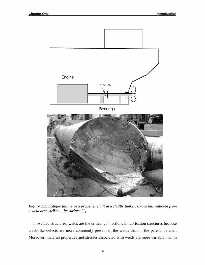
Fatigue is the main cause of damage, followed by groups that can be designated as
accidental damage. Figure 1.1 shows a fatigue failure of a propeller shaft in a shuttle tanker.
Chapter One Introduction
3
The fracture occurred in the intermediate part of the shaft. The crack started from the
surface of the shaft due to a weld arch strike. The fatigue surface is characterized by its
smooth appearance with almost no plastic strain. At several stages during crack
propagation, marks which are due to low stress variations are left as traces on the fatigue
surface. These so-called beach marks correspond to changes in the fatigue loading; the
crack front will make a mark during the time of slow growth due to smaller stress cycles.
These marks are analogous to the dark winter rings found in the cross section of a tree. As
can be seen, the beach marks have a typical semi-elliptical shape indicating the position of
the crack front at various stages during the crack propagation. When the fatigue crack has
reached the size of about three-quarters of the shaft diameter (D = 360 mm), the final
fracture has occurred due to lack of the remaining ligament of the shaft cross section. It is a
ductile fracture governed by the maximum occurring shear stress [1].
Chapter One Introduction
4
Figure 1.1: Fatigue failure in a propeller shaft in a shuttle tanker. Crack has initiated from a weld arch strike at the surface [1]
In welded structures, welds are the critical connections in fabrication structures because
crack-like defects are more commonly present in the welds than in the parent material.
Moreover, material properties and stresses associated with welds are more variable than in
Chapter One Introduction
5
parent material. Thus, failure is more likely to occur at welds. In 1968, a catastrophic
failure occurred in a 350 MW turbine at the intermediate pressure loop-pipe to steam chest
weldment in U.K. The failure was traced to the circumferential cracking at the interface
between the 1 Cr-1 Mo-0.3 V cast steam chest and the 2 ¼ Cr-1 Mo weld metal. The crack
was believed to have been introduced during the heat treatment operation or within a short
time of commissioning of the turbine. A fracture mechanics approach was adopted to
analyse the safety of the components and those found not suitable were replaced. Thus,
application of fracture mechanics can be applied in the broad area of determining the
acceptable defect’s size.
In the same time the incidence of fatigue cracking has become a problem of critical
importance. Welded joints have normally complicated geometries and are subjected to
complicated service environments and stress conditions which may finally lead to early
fatigue cracking.
Fatigue and fracture analysis of cracks are therefore of great practical interest and
require the accurate determination of the stress state at a crack tip which is defined in terms
of the stress intensity factor, SIF for the case under analysis. They are necessary for
calculating the fatigue life.
1.3. Failure of Welded Joints
Welds can introduce severe stress concentrations which differ from one structural
element to another [1, 2].
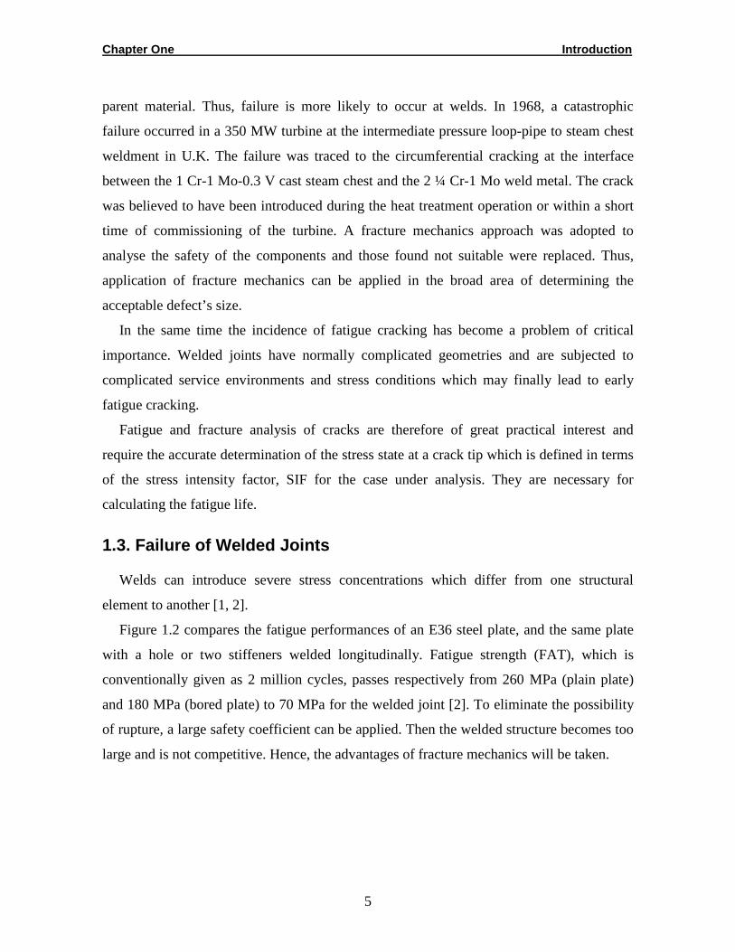
Figure 1.2 compares the fatigue performances of an E36 steel plate, and the same plate
with a hole or two stiffeners welded longitudinally. Fatigue strength (FAT), which is
conventionally given as 2 million cycles, passes respectively from 260 MPa (plain plate)
and 180 MPa (bored plate) to 70 MPa for the welded joint [2]. To eliminate the possibility
of rupture, a large safety coefficient can be applied. Then the welded structure becomes too
large and is not competitive. Hence, the advantages of fracture mechanics will be taken.
Chapter One Introduction
6
Figure 1.2: Fatigue life curves for various details [1, 2]
Welding operation result in the existence of stress concentrated areas where fatigue
crack may originate and expand from. Welded joint geometries, internal defects (lack of
penetration, LOP) or external defects (undercuts, slag inclusions), and loading types will
determine the crack path (CP) and fatigue life of a specific joint. The most traditional
welded joints are described below.
1.3.1. Butt Welded Joints
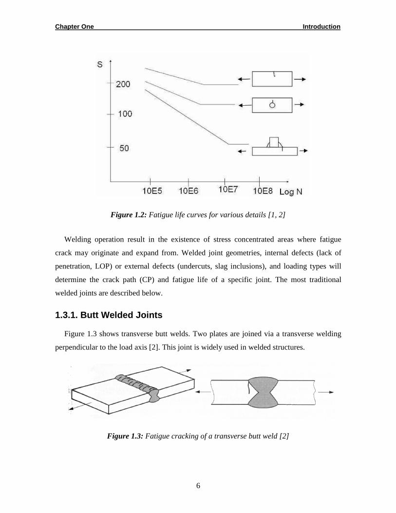
Figure 1.3 shows transverse butt welds. Two plates are joined via a transverse welding
perpendicular to the load axis [2]. This joint is widely used in welded structures.
Figure 1.3: Fatigue cracking of a transverse butt weld [2]
Chapter One Introduction
7
For this type of joint, the fatigue crack starts at the weld toe and propagates through the
thickness of the sheet, perpendicular to the load direction. The crack is thus not the result of
a defect including welding or bad properties of the deposit metal, but the consequence of
stress concentrations at the weld toe.
In this type of butt welded joint, the influence of the shape of the weld bead is important
for determining the endurance characteristics of the joint. This depends greatly on the
welding conditions.
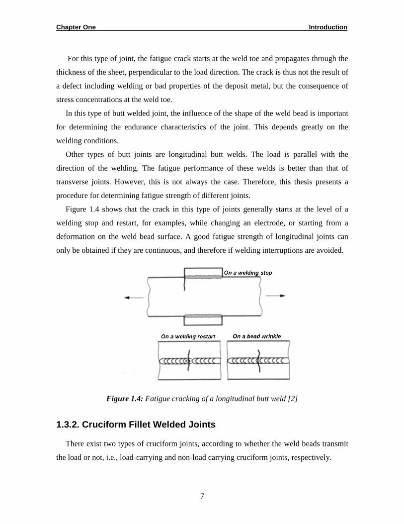
Other types of butt joints are longitudinal butt welds. The load is parallel with the
direction of the welding. The fatigue performance of these welds is better than that of
transverse joints. However, this is not always the case. Therefore, this thesis presents a
procedure for determining fatigue strength of different joints.
Figure 1.4 shows that the crack in this type of joints generally starts at the level of a
welding stop and restart, for examples, while changing an electrode, or starting from a
deformation on the weld bead surface. A good fatigue strength of longitudinal joints can
only be obtained if they are continuous, and therefore if welding interruptions are avoided.
Figure 1.4: Fatigue cracking of a longitudinal butt weld [2]
1.3.2. Cruciform Fillet Welded Joints
There exist two types of cruciform joints, according to whether the weld beads transmit
the load or not, i.e., load-carrying and non-load carrying cruciform joints, respectively.
Chapter One Introduction
8
1.3.2.1. Non-Load Carrying Fillet Weld
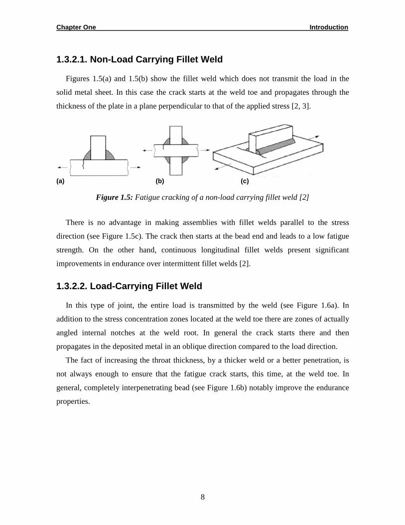
Figures 1.5(a) and 1.5(b) show the fillet weld which does not transmit the load in the
solid metal sheet. In this case the crack starts at the weld toe and propagates through the
thickness of the plate in a plane perpendicular to that of the applied stress [2, 3].
(a) (b) (c)
Figure 1.5: Fatigue cracking of a non-load carrying fillet weld [2]
There is no advantage in making assemblies with fillet welds parallel to the stress
direction (see Figure 1.5c). The crack then starts at the bead end and leads to a low fatigue
strength. On the other hand, continuous longitudinal fillet welds present significant
improvements in endurance over intermittent fillet welds [2].
1.3.2.2. Load-Carrying Fillet Weld
In this type of joint, the entire load is transmitted by the weld (see Figure 1.6a). In
addition to the stress concentration zones located at the weld toe there are zones of actually
angled internal notches at the weld root. In general the crack starts there and then
propagates in the deposited metal in an oblique direction compared to the load direction.
The fact of increasing the throat thickness, by a thicker weld or a better penetration, is
not always enough to ensure that the fatigue crack starts, this time, at the weld toe. In
general, completely interpenetrating bead (see Figure 1.6b) notably improve the endurance
properties.

Chapter One Introduction
9
(a) (b)
Figure 1.6: Fatigue cracking of a load-carrying fillet weld [2]: (a) root crack; (b) toe crack
1.4. Concept of Fracture Mechanics Methods
With the consideration of welding as the major method of fabrication, cracking in the
heat-affected zone (HAZ) and weld metal has become a serious problem particularly in
large and continuous structures. The inevitable cracking in weld joints makes the estimation
of initial crack length (ai) to be very important to calculate the time of fatigue crack growth
propagation (FCG). In particular, the fact that fatigue cracks initiate very readily at the weld
toe, virtually eliminating a crack initiation period and giving a fatigue life which is spent
largely in crack propagation [4].
The weld cracks are induced due to various factors. For example, one of the major
problems in the welding of steels is the type of cracking which is generally known as
hydrogen induced cold cracking. At high carbon levels, the HAZ cracking was severe
because of the formation of brittle martensite as a result of rapid cooling in welding. In the
presence of hydrogen gross cracking is inevitable. The combination between the residual
stress and corrosive media also produce a cracking called stress corrosion cracking.
Regardless the reasons for crack formations, fracture mechanics is mostly used in life
prediction of a welded structure with an existing crack or under assumptions of the
presence of a crack not found by non-destructive testing.
The initiation phase is assumed negligible for welded joints in the fracture mechanics
approach and the life calculation is based upon a stress intensity factor SIF, which accounts
for the magnitude of stress, crack size and joint details geometries.
Chapter One Introduction
10
Regarding the first crack nucleation phase, it is possible to use a local, cyclic stress
strain approach at the weld notch to calculate the time to crack initiation. However, the
same practical result can be obtained by a fracture mechanics approach using a fictitious,
small, initial crack size [1].
It is to be interested that these small, initial cracks must be regarded as fictitious cracks
chosen to make LEFM describe the entire fatigue process. They are not real, physical
cracks (flaws, intrusions) created by the welding procedures. It is therefore difficult to
relate the derived model to actual detected flaws in the weld. Furthermore, the initial cracks
are often so small that LEFM is not applicable, typical values being from ai= 0.01 to 0.05
mm [1], or even 0.15 which is recommended by IIW [3, 34]. This crack size is close to the
microstructural features of the material. Ordinary structural steel qualities often have a
grains size near 0.01 mm. Therefore, it is to be emphasized that it may be dubious to apply
LEFM at crack depths of less than 0.1 mm. Before this stage the crack initiation
phenomenon is probably better modeled by the Coffin and Manson equation. This equation
is based on a local stress-strain approach [1]. The J-integral method and Paris’ crack growth
law have used also to predict crack growth rates and identical fatigue behaviour in short
crack propagation. Nevertheless, fracture mechanics approach is used in this work, and the
evaluation of the ability of this tool in fatigue life calculation is presented.
1.5. Residual Stresses in Welding
Residual stresses are internal forces in equilibrium themselves. These stresses are
produced due to various manufacturing processes such as forging, casting, rolling,
machining, cutting, heat treatment, surface treatment, hardening and shot peening. The
formation of some microstructures such as bainite and martensite lead also to residual
stresses. Moreover, residual stresses develop due to the welding processes which are
concerned in the current work.
Residual stresses are important in fatigue life, stress corrosion resistance, dimensional
stability and brittle fracture. In general, the effect of residual stresses may either be
beneficial or detrimental, depending on magnitude, sign and distribution of the stresses
with respect to the load-induced stresses. Tensile residual stresses are detrimental and often
in the magnitude of the materials yield strength. The tensile residual stresses will reduce the

Chapter One Introduction
11
fatigue life of the structure by increasing the growth of a fatigue crack, while compressive
residual stresses are very beneficial and will decrease the fatigue crack growth rate [5-9].
In welding the residual stresses are developed due to non-uniform thermal expansion
caused by the local heating of the structure. The yield stress is strongly temperature
dependent, so the maximum stress at any point in the metal depends on the local
temperature. The temperature will vary in three dimensions as the weld progresses, through
the thickness, across the width of the weld and along the length. This gives rise to a
complex stress distribution throughout the weldment which will be further complicated as a
weld subsequently is deposited.
Residual stresses will never contribute to failure by plastic collapse but they will make a
significant contribution to failure by brittle fracture (linear elastic fracture), or stress
corrosion cracking in susceptible environments. Thus to assess the influence of the residual
stresses on the failure of a weldment, their distribution must be known.
It is duly expected that in a notched specimen not only the phenomenon of the
redistribution of welding residual stresses with fatigue crack extension occurs but also the
phenomenon of the relaxation of welding residual stress with the fatigue loading might
possibly occur at the same time and this would make the problem quite difficult [10].
Therefore, the effects of applied stress ratio (Rapp) in correlation with residual stress ratio
(Rres) and residual stresses distribution have to be investigated.
1.6. Objectives and Scope
From the design point of view, fatigue properties of welded structures such as the initial
crack length, the final crack length, crack growth data and fatigue strength curve (S-N or
Wöhler curve) should be determined accurately. Then, the fatigue life of welded structures
can be correctly evaluated. Unfortunately, the real value of crack lengths and crack growth
properties according to notch cases are not known sufficiently for most cases.
The welding standards contain descriptions of a number of possible weld geometries,
with limits for the accepted dimensions of the defects. The fatigue life calculation of
different weld classes as based on fracture mechanics approach requires fixed values of
crack length and SIFs. The latter can be calculated due to applied load and due to residual
stress.
Chapter One Introduction
12
Limited work is published for the calculation of SIFs under residual stress fields [11]
and the effect of residual stresses on the crack growth life.
The aim of this work is to calculate the fatigue strength of notch cases using fracture
mechanics based method and comparison with the solutions of the International Institute of
Welding (IIW) [3], Eurocode 3 [12], Germanischer Lloyd Aktiengesellschaft (GL) [13] and
British Standards Institution (BSI) [14].
The fatigue strengths have been calculated based on real values of crack length for each
notch case that is calculated in this work. Moreover, the distributions of residual stresses
and their influences on crack growth life were determined. In addition, the correlation
between the residual stress distribution effect and load ratio R was investigated.
With the current fracture mechanics models, different notch cases could be defined
including fatigue strength that is called FAT (fatigue strength at 2 million cycles) and
residual stress distributions. The fatigue strength for unknown notch cases not listed yet in
the standards can be calculated under the effect of different weld geometries and different
residual stress profiles.
1.7. Outline of the Thesis
This study includes fatigue life calculations and comparisons with literature using
fracture mechanics methods and is divided into six chapters.
Chapter One gives a brief Introduction to the main topics of the thesis.
In Chapter Two, a comprehensive Literature Review for fatigue life of welded joints,
fracture mechanics approach and residual stresses is presented. The focus lies on LEFM
(linear elastic fracture mechanics), which is used in this thesis. The Modeling of Welded
Joints and SIF Calculation are thoroughly described in Chapter Three.
In Chapter Four, Fatigue Life Calculations and Verifications, analytical techniques and
procedures that are used to predict the fatigue life of various structures are described in
detail.
Data published in the open literature and the fatigue test results are presented as a part of
comparisons and experimental verifications in the fourth chapter. Re-analysis and re-
calculation of notch cases in the literature and standards are shown also in the fourth
chapter. A discussion of Residual Stresses in Welded Joints is given in Chapter Five.
Chapter One Introduction
13
Finally, Conclusions and Recommendations for Future Work are presented in Chapter Six.
The evaluation of design codes is restricted to IIW, BS, Eurocode 3, and GL
recommendations.
1.8. The Present Work
The fatigue testing of welded joints and large scale structures is time consuming and
expensive. Therefore, the analytical procedures and software have been developed to
predict the crack initiation, crack path and propagation time. However, the initiation time
for cracks in weld joints is neglected in fracture mechanics approaches by supposing an
initial crack length.
Linear elastic fracture mechanics can then be used to calculate the propagation portion
of the total life by integrating the crack growth rate (da/dN)-stress intensity factor (∆K)
relation from a specific crack size to the critical crack size at fracture. However, the
application of ordinary fracture mechanics parameters like K-factor to very small cracks
(below 1 mm) is criticized (particularly in fatigue).
For each case the geometry is modeled and SIFs are obtained to calculate the fatigue
life. The weld joint geometry with an initial crack is modeled in the FEM program
FRANC2D. In this program a crack is propagated automatically or step by step according
to the maximum stress direction. For every crack length, the SIFs were calculated. The
results have been used to determine the SIF as function of crack length for the particular
case in form of a polynomial function with suitable order. These FE results were
benchmarked for the effects of mesh size, mesh type, mesh density, crack increment and
effect of symmetry to evaluate the reliability of current FE mode in SIFs calculations.
The introduced function has been used for calculating the fatigue life by using fracture
mechanics method. The life was assumed to be finished when the crack reaches half the
sheet thickness; however, the final crack length has negligible effect on fatigue life. All
steps of the procedure were described thoroughly in the following chapters.
The following points summarize procedures of the current approach:
1. FE modeling that gives accurate stress intensity factors.
2. With knowledge of the stress intensity factors at different crack depths, it was possible to
make curve fits between SIF and crack length, then calculate KI (a) for different loading
Chapter One Introduction
14
due to the linear relation between KI and load. Also the effects of crack increment and mesh
elements have been studied to give satisfactory results.
3. Insert the polynomial equation into fatigue life formula (da/dN-∆K) and carry out the
numerical integration to calculate the expected fatigue life of the specimens and construct
the fatigue life curve (S-N).
4. Carry out the backward calculations for the fatigue life curve as compared with known
cases from the standards for the value of fatigue strength life (FAT). Crack growth
parameters are fixed which give coalescence between the fatigue life curve from the current
calculations and those from standards.
5. Determine the initial crack length for different notch cases and reveal the typical length
which would give satisfactory results for specific types of cracking joints and loading
conditions. Crack growth parameters and final crack lengths have been fixed while the
initial crack was manipulated. Final crack length was chosen to be equal to one-half of the
plate thickness.
6. Investigate the effect of the residual stresses on the crack propagation life based on the
calculated parameters from point 5.
7. Investigate the effect of applied stress ratio (Rapp) and residual stress ratio (Rres) on
fatigue life by incorporating them in addition to residual stress distributions into the fatigue
life formula.
The incorporation all above steps in one approach was the task of the current work.
These approaches are validated and compared through the following chapters of this work.

Chapter Two Literature Review
15
Chapter Two
LITERATURE REVIEW
2.1. Introduction
With welded joints, stress concentrations occur at the weld toe and at the weld root,
which make these regions the points from which fatigue cracks may initiate. To calculate
the fatigue life of welded structures and to analyze the progress of these cracks, fracture
mechanics technique is used.
In most cases, the welded components are designed using S-N nominal curves which
predict only the fatigue life of the component. However, in weldment, the fatigue crack
propagation was more significant and takes a majority of total fatigue life.
Since the crack initiation occupies only a small portion of the life it can be assumed
negligible. The fracture mechanics method is suitable for assessment of fatigue life and
inspection intervals in weld structures.
2.2. Fracture Mechanics of Fillet Welded Joints
The inevitable parameter in fracture mechanics is the stress intensity factor (SIF) which
is used in fatigue life calculation. SIF tightly knit with the fracture mechanics to predict the
stress state near the tip of a crack caused by a remote load which should take into account
the residual stresses in conjunction with geometry.
Nykänen et al. [15] investigated the fatigue behavior of 12 common types of welded
joints parametrically and the tools which would allow more precise assessment of the effect
of dimensional variations on the fatigue strength (FAT) were given [15]. They mentioned
that in parallel joints toe cracks and lack of penetration (LOP) are frequently encountered
defects in fillet welded joints. Toe cracks occur because of the stress concentration in the
weld toe region, while LOP results from inaccessibility of the root region during welding.
Chapter Two Literature Review
16
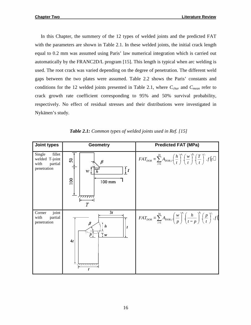
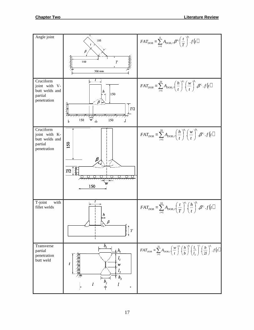
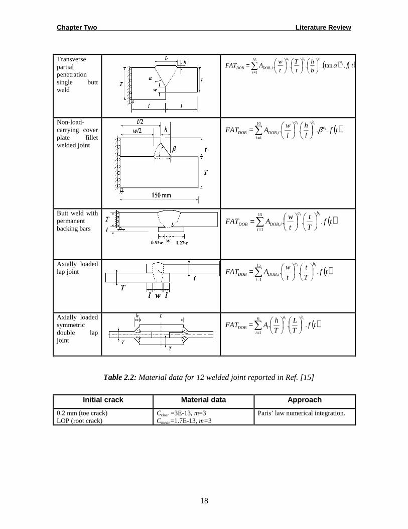
In this Chapter, the summery of the 12 types of welded joints and the predicted FAT
with the parameters are shown in Table 2.1. In these welded joints, the initial crack length
equal to 0.2 mm was assumed using Paris’ law numerical integration which is carried out
automatically by the FRANC2D/L program [15]. This length is typical when arc welding is
used. The root crack was varied depending on the degree of penetration. The different weld
gaps between the two plates were assumed. Table 2.2 shows the Paris’ constants and
conditions for the 12 welded joints presented in Table 2.1, where Cchar and Cmean refer to
crack growth rate coefficient corresponding to 95% and 50% survival probability,
respectively. No effect of residual stresses and their distributions were investigated in
Nykänen’s study.
Table 2.1: Common types of welded joints used in Ref. [15]
Joint types Geometry Predicted FAT (MPa)
Single fillet welded T-joint with partial penetration
( )tft
T
t
w
t
hAFAT
iii cba
iiDOBDOB ....
20
1,
=∑=
Corner joint with partial penetration
(ft
p
pt
h
p
wAFAT
iii cba
iiDOBDOB ....
56
1,
−
=∑=
Chapter Two Literature Review
17
Angle joint
( )tfT
tAFAT
i
i
ba
iiDOBDOB ..
6
1,
=∑=
β
Cruciform joint with V-butt welds and partial penetration
( )tft
w
t
hAFAT i
ii
cba
iiDOBDOB ....
20
1, β
=∑=
Cruciform joint with K-butt welds and partial penetration
( )tft
w
t
hAFAT i
ii
cba
iiDOBDOB ....
20
1, β
=∑=
T-joint with fillet welds
( )tft
h
T
tAFAT i
ii
cba
iiDOBDOB ....
10
1, β
=∑=
Transverse partial penetration butt weld
( )tfl
b
l
l
b
h
t
wAFAT
iiii dcba
iiDOBDOB .
2....
2
135
1,
=∑=
Chapter Two Literature Review
18
Transverse partial penetration single butt weld
( ) ( )tfb
h
t
T
t
wAFAT i
iiid
cba
iiDOBDOB .tan....
35
1, α
=∑=
Non-load-carrying cover plate fillet welded joint
( )tfl
h
l
wAFAT i
ii
cba
iiDOBDOB ....
10
1, β
=∑=
Butt weld with permanent backing bars
( )tfT
t
t
wAFAT
ii ba
iiDOBDOB ...
15
1,
=∑=
Axially loaded lap joint
( )tfT
t
t
wAFAT
ii ba
iiDOBDOB ...
15
1,
=∑=
Axially loaded symmetric double lap joint
( )tfT
L
T
hAFAT
ii ba
iiDOB ...
6
1
=∑=
Table 2.2: Material data for 12 welded joint reported in Ref. [15]
Initial crack Material data Approach
0.2 mm (toe crack) LOP (root crack)
Cchar =3E-13, m=3 Cmean=1.7E-13, m=3
Paris’ law numerical integration.
Chapter Two Literature Review
19
From literature [16-18], it is evident that most of the investigations on fatigue life
prediction of the fillet welded joints are based on toe failure. Some other studies have
considered the fatigue behavior of fillet welded joints failing from the root region.
Motarjemi et al. [19], Balasubramanian and Guha [20], Frank and Fisher [21], Usami
and Kusumoto [22], have also studied the fatigue behavior and SIF of cruciform and T
welded joints of carbon steels failing from the root (LOP).
Motarjemi et al. [19] evaluated SIFs at the crack roots of T and cruciform welded joints
with LOP defects by FEM using ABAQUS package to analyze the different joint
geometries. They found that the SIFs for cruciform welded joints were nearly always higher
than those for the comparable T-welded joints.
Fatigue failure typically takes place at sites of high stress in either the base material or
weldments. Weld toe contains the stress concentration site and small crack-like
discontinuities [4, 23-26]. Such cracks tend to be along the line normal to the transverse
stress.
Considering fatigue crack growth in welded joints, the percentage of the crack
propagation phase in the total fatigue life depends very much on the quality of the weld
comprising; weld geometry, initial defects in the weld, weld residual stresses and local
stress conditions. Since welding defects can frequently exist in the vicinity of weldments,
local stress concentrations around discontinuities and weld defects are fairly common.
These crack-like defects begin to grow almost immediately when subjected to external
cyclic fatigue loads, so that, for welded joints, the total fatigue life is mainly dominated by
the crack propagation phase. Moreover, weld defects that were the source of crack initiation
and growth were characterized. Internal discontinuities include porosity, entrapped oxides,
and lack of fusion sites located in the longitudinal fillet welds and the groove welds [27].
Therefore, fracture mechanics approach assumes the existence of an initial crack ai. It
can be used to predict fatigue life and strength of the growth of the crack to its final size af.
For welds in structural metals, crack initiation occupies only a small fraction of the life and
it can be assumed negligible [8, 28]. Therefore, this method is suitable for assessment of
fatigue life, inspection intervals, and crack-like weld imperfections that are likely present in
weld joints. Initial cracks used in fatigue analyses are often in the range of 0.05-0.2 mm
[29]. However, Engesvik [30] has also analyzed the fatigue life of welded joints and
Chapter Two Literature Review
20
concluded that it may be dubious to apply LEFM at crack depths less than 0.1 mm.
Nevertheless, this value can vary depending on the welding operation parameters, geometry
and materials properties. Lindqvist [31] showed a 12 mm specimen’s fracture surface after
it was fatigue tested and afterwards broken up. Probably there were several small cracks
along the weld toe. When the cracks grew in the direction normal to the applied load, they
united into one large semi-elliptical crack. For load-carrying cruciform welded joints, lack
of penetration (LOP) is considered to act as initial crack. Initial crack, ai is usually
measured or approximated to 0.1-0.2 mm for welds. Table 2.3 shows the parameters used in
Lindqvist’s study [31].
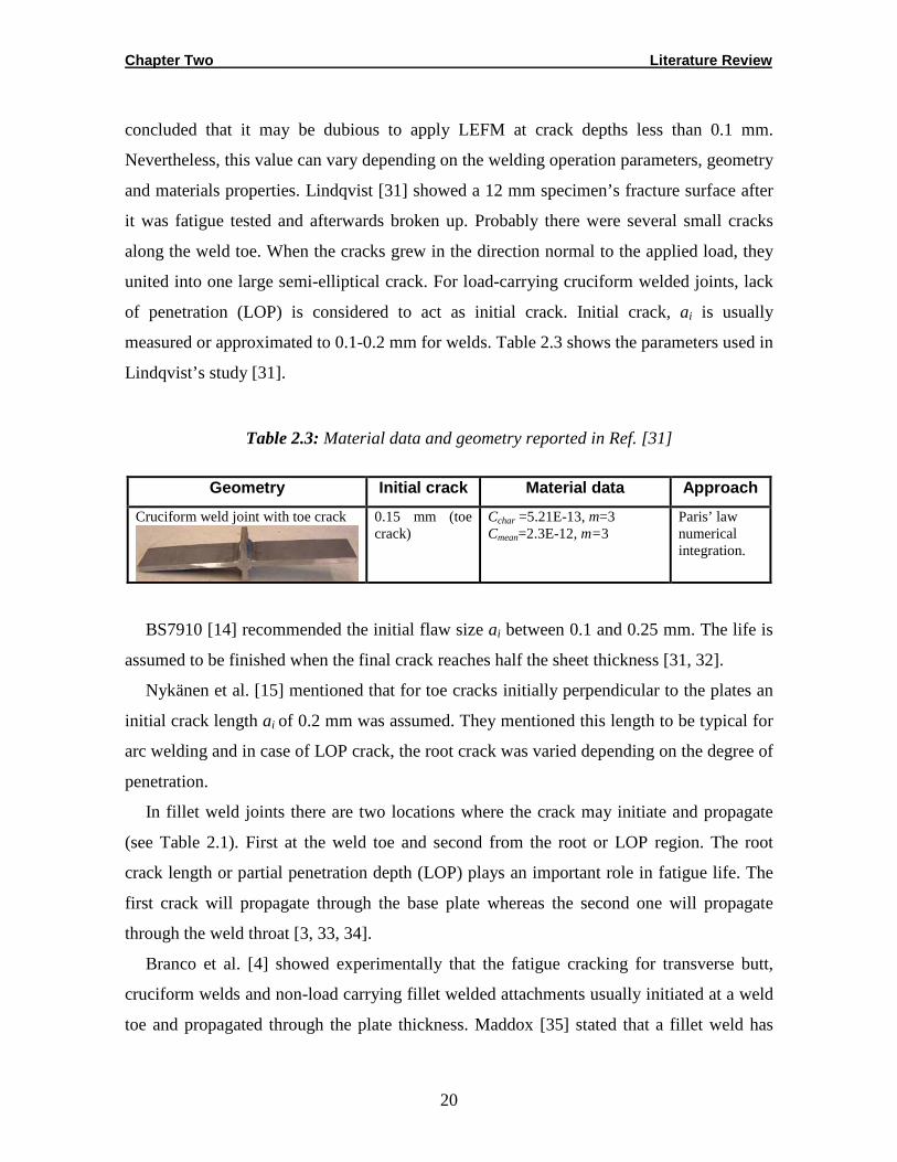
Table 2.3: Material data and geometry reported in Ref. [31]
Geometry Initial crack Material data Approach
Cruciform weld joint with toe crack
0.15 mm (toe crack)
Cchar =5.21E-13, m=3 Cmean=2.3E-12, m=3
Paris’ law numerical integration.
BS7910 [14] recommended the initial flaw size ai between 0.1 and 0.25 mm. The life is
assumed to be finished when the final crack reaches half the sheet thickness [31, 32].
Nykänen et al. [15] mentioned that for toe cracks initially perpendicular to the plates an
initial crack length ai of 0.2 mm was assumed. They mentioned this length to be typical for
arc welding and in case of LOP crack, the root crack was varied depending on the degree of
penetration.
In fillet weld joints there are two locations where the crack may initiate and propagate
(see Table 2.1). First at the weld toe and second from the root or LOP region. The root
crack length or partial penetration depth (LOP) plays an important role in fatigue life. The
first crack will propagate through the base plate whereas the second one will propagate
through the weld throat [3, 33, 34].
Branco et al. [4] showed experimentally that the fatigue cracking for transverse butt,
cruciform welds and non-load carrying fillet welded attachments usually initiated at a weld
toe and propagated through the plate thickness. Maddox [35] stated that a fillet weld has
Chapter Two Literature Review
21
small sharp defects along the weld toe from which fatigue cracks propagate. This effect
combines with the stress concentration so that the fatigue life is effective in propagating the
crack.
In most cases toe cracks have been considered [4, 31, 32, 36, 37] because they are easier
to observe with the naked eye as well as with dye penetration tests. In addition to high
stress concentration, the tensile residual stresses are located in this point. The tensile
residual stresses of yield strength magnitude exist at the weld toe regions reducing the
fatigue life [24].
Singh et al. [38] presented the findings of a study of the axial fatigue performance of
AISI 304L load-carrying cruciform joints which failed in the weld metal with and without
cryogenic treatment. The fatigue properties of cryogenically treated samples have shown
improvement due to strain induced martensite that formed during cryogenic treatment and
the associated generation of compressive stresses in the weld metal.
Hou et al. [39] mentioned that a crack depth of 0.25 mm was commonly used as
terminate of crack initiation phase. Many strain gages placed along the weld direction in T-
joint, near the weld toe and the size and location of initiated surface cracks by was detected
change in the strain gages readings. They claimed that cracks with a depth of 0.5 mm or
even smaller could be detected. They recorded the total fatigue life of the T-joints and the
crack propagation life from a crack depth of 0.5 mm to the final failure. They showed that
fillet weld joints like T-joint have high stress concentrations at the weld toe. Therefore, it is
easier to initiate a crack from the weld toe, hence, the value of initial number to total
number of cycle (NI/NT) become smaller.
Balasubramanian et al. [20] analyzed the influences of two welding processes, namely,
shielded metal arc welding (SMAW) and flux cored arc welding (FCAW), on fatigue life of
cruciform joints containing LOP defects.
Finally, it should be mentioned that the lists of fatigue strength of fillet welded joints
failing from toe and root cracks, respectively, are presented in the International Institute of
Welding (IIW) [3, 34], Germanischer Lloyd Aktiengesellschaft (GL) [13], and British
Standard Institution (BSI) [14].
Chapter Two Literature Review
22
2.3. Crack Propagation Curve
The fatigue of welded joints is a vast area and gives many possibilities for research. It
has been found from experience that most common failures of engineering structures such
as welded components are associated with fatigue crack growth caused by cyclic loading.
Engineering analysis of fatigue crack growth is frequently required for structural design,
such as in Damage Tolerance Design (DTD) and residual life prediction when an
unexpected fatigue crack is found in a component of engineering structure. For analysis, the
fatigue life of welded structures can be divided into two parts: crack initiation phase and
propagation phase. The initiation life is defined by the number of loading or straining
cycles, Ni, required to develop a crack of some specific size, ai. The propagation stage then
corresponds to that portion of the total cyclic life, Np, which involves growth of that crack
to some critical dimension at fracture, af. Hence NT=Ni+Np, where NT, is the total fatigue
life. Therefore, fatigue crack propagation behavior is typically described in terms of crack
growth rate or crack length extension per cycle of loading (da/dN) plotted against the SIF
range (∆K) or the change in SIF from the maximum to the minimum load (see Figure 2.1)
[28].
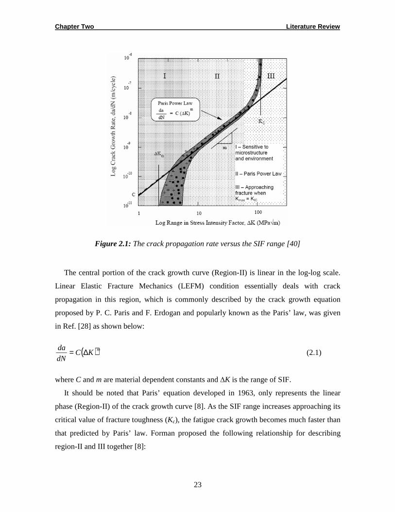
The first region (I) in Figure 2.1 is referred to as the near threshold region. It indicates a
threshold value, below which there is no observable crack growth. The second region (II) is
a linear region, which is known today as the Paris’ law region. During this period, fatigue
crack growth (FCG) corresponds to stable macroscopic crack growth. In the third region
(III), FCG is very high as it approaches instability and point of fracture. There is little FCG
life involved and it is primarily controlled by the fracture toughness (KIC). The main part of
the log-log plot of da/dN versus ∆K that is of most concern in most works is the Paris’
region (Region-II). This region describes the crack growth behaviour using the relationship
between cyclic crack growth rate da/dN, and the stress intensity range, ∆K [9, 40].
Chapter Two Literature Review
23
Figure 2.1: The crack propagation rate versus the SIF range [40]
The central portion of the crack growth curve (Region-II) is linear in the log-log scale.
Linear Elastic Fracture Mechanics (LEFM) condition essentially deals with crack
propagation in this region, which is commonly described by the crack growth equation
proposed by P. C. Paris and F. Erdogan and popularly known as the Paris’ law, was given
in Ref. [28] as shown below:
( )mKCdN
da ∆= (2.1)
where C and m are material dependent constants and ∆K is the range of SIF.
It should be noted that Paris’ equation developed in 1963, only represents the linear
phase (Region-II) of the crack growth curve [8]. As the SIF range increases approaching its
critical value of fracture toughness (Kc), the fatigue crack growth becomes much faster than
that predicted by Paris’ law. Forman proposed the following relationship for describing
region-II and III together [8]:
Chapter Two Literature Review
24
KKR
KC
dN
da
c
m
∆−−∆=)1(
)( (2.2)
where R is the stress ratio, equal to σmin/σmax.
Note that the above relationship (2.2) accounts for stress ratio, R effects, while Paris law
assumes that da/dN depends only on ∆K. Based on the above relationship, fatigue crack
propagation life can be predicted by integrating both sides of these functions if a suitable
SIF solution is obtained.
It is to be emphasized that fatigue crack growth equation which is sensitive to R like
NASGRO equation is recommended to use, or add to the Paris’ model the crack closure
phenomenon or any other model accounting for the state of affairs at the crack tip.
The equation is used in the most recent release of the crack growth prediction program,
NASGRO. The NASGRO equation is written as:
q
c
p
thn
ESA
K
K
K
K
KR
fC
dN
da
−
∆
∆−
∆
−−=
max1
1
1
1 (2.3)
where CESA and n are empirical parameters describing the linear region of the curve (similar
to the Paris’ model), and p and q are empirical constants describing the curvature in fatigue
crack growth rate (FCG) data that occur near threshold (Region-I) and near instability
(Region-III), respectively. The Newman’s effective stress ratio (f), the threshold value of
SIF range for a given R, (∆Kth) and the critical SIF (Kc) are presented in Chapter Four. The
unit for the fatigue crack growth rate (FCG) da/dN is mm/cycle, and the SIF range ∆K is
MPa (m)1/2.
Research to date used the modified Paris’ or Forman’ law and incorporating them with
residual stress intensity factor and total SIF to calculate lives which consider only the linear
region of crack growth curve.
Chapter Two Literature Review
25
2.4. Simulation of Fatigue Crack Growth
In spite of the fact that several SIF handbooks have been published, it is still difficult to
find solutions adequate to many welded configurations [27, 41]. This is mainly due to a
wide variety of complex welded geometries, loading systems and the suitable solutions are
not always available.
When no analytical solutions are available, several modeling methods may be used. The
most modern ways to solve the SIFs are Finite Element (FE) or Boundary Element (BE)
software. Automatic meshing during the crack growth is included in some software.
The finite element method (FEM) has been widely employed for solving linear elastic
and elastic-plastic fracture problems. The evaluation of SIFs in 2D geometries by FEM is a
technique widely used for non-standard crack configurations. As regards to through
thickness weld toe cracks, no 3-D analysis results have yet been reported to the author’s
knowledge.
Over the years, the complexity of problems increased significantly and that makes it
important to convert and provide a more useful method that can be used for fatigue
problems.
Although the complexity of models has increased, the first applications were for
relatively simple purposes such as the determination of SIFs for different crack
configurations and different joint geometries.
Andersen [7] presented models of 2-dimensional crack simulation. In addition, the
effects of residual stresses have been studied using the FE-based optimization program
ODESSY. The stress intensity state at each location of the crack tip was used to predict the
direction of the next crack increment. The procedure involved re-meshing of the domain
containing the continuously changing crack geometry and a model for prediction of the
crack growth direction. Thus, the procedure was used to simulate the crack growth. The
obtained results showed a reasonable agreement with experimentally obtained data. The
weakness of the approach was the missing ability of the re-meshing algorithm to produce a
high quality mesh in the domain around the crack tip.
The main problem of using FE-based software is that the simulation of the crack growth
is very time consuming. While the main problem using BE method is that the engineers are
Chapter Two Literature Review
26
not familiar with this method and the solving of the BE model is not as fast as the FEM
[42].
Caccese et al. [23] performed FE analyses on the cruciform-shaped test articles to
ascertain the stress concentration factor for various shaped fillet geometries. The ANSYSTM
FE program was used for this purpose. Results of the FE analysis were processed using
several analytical methods and these data were used to estimate the relative change in
fatigue life due to the geometry of the fillet. Since it is desirable to use these methods with
a multitude of weld profiles, the FE method was chosen for the analysis procedure to
determine the stress concentration factor.
In ANSYS, to model the crack a small cut in the geometry is performed. This means that
there is a relatively small distance between the points at the opening of the crack. In all
models, the growth of the crack is perpendicular to the horizontal sheet. Crack growth is
simulated by moving the crack tip key point into the material. Moreover, the crack can be
difficult to mesh because the elements must be relatively small near the crack tip. In order
to get around that problem the total area of the sheet is divided into smaller areas. Since the
elements around the crack tip must be relatively small and larger elements are used far
away from the crack it is extremely time consuming to use these small elements’ model.
Problems may occur in the transition area between smaller and larger elements. This is
done by creating a box around the crack tip, containing small elements. Although large
efforts have been made to control the meshes, sometimes some bad elements appear around
the box.
Therefore, Karlsson [32] found that using a smaller element side length on the global
areas, 0.2 mm instead of 1 mm, the badly shaped elements disappear. The calculation time,
however, is about 10 to 20 times longer and the calculated SIFs improve less than 1.5%.
Since several geometries are to be calculated, the coarser mesh is used to save time.
Boundary Element Analysis System software (BEASY) [43] which is now a simple
extension of the standard stress analysis is performed by engineers. Simply select the shape,
size, and location of the crack and BEASY will automatically re-mesh the model to include
the crack and compute the stress intensity data.
Moreover, BEASY not only provides stress intensity data but can also predict how the
crack will grow and provide the automatic crack growth re-meshing which is automatically
Chapter Two Literature Review
27
performed by BEASY where necessary. The procedure is highly automated with a crack
growth wizard guiding the user. High accuracy historically, SIF and crack growth data have
been approximated using standard reference solutions.
Fricke et al. [44, 45] performed BEM analysis using the code BEASY where the
displacement method is used for the SIFs solution. The crack propagation has been
calculated based on Paris’ crack growth law using the computed SIFs along the crack front.
It can be seen that the highest crack propagation occurs at two points namely at the end of
the root gap and close to the corner.
2.5. Fracture Analysis Code
The FE program (FRANC2D) was developed by the Cornell Fracture Group from
Cornell University, USA [46]. FRANC provides higher time saving and is more familiar
with application and mesh generation.
The analysis was undertaken based on the assumption of an initially isotropic elastic
material, in which a crack was subsequently allowed to form and grow according to a
fracture criterion. Therefore, it combines with BEASY by the easy crack modeling and
meshing.
In FRANC there is no reality for using the box which is used in ANSYS and there is not
necessarily to use the fine mesh near the crack tip thereby saving time. It can be shown that
FRANC has advantages over other FE software to calculate SIFs. It can be applied for
mechanical component crack growing in addition to civil engineering applications.
Moreover, FRANC2D can be used to represent the crack geometry in a fuselage, and to
simulate crack interaction with various structural elements. However, Mashiri et al. [25]
discussed the nature of 2-dimensional models and they assume that undercut is continuous
throughout the whole length of the weld toe. This should give a conservative value of
fatigue crack propagation life as compared to real cruciform joints under tensile cyclic
loading where cracks can initiate at multiple points along the weld toe of the cruciform
joints and propagate before coalescence occurs.
The simulation of fatigue assessment method by FEM using FRANC2D depends on
SIFs. The analysis can be undertaken using a version of the program downloaded from the
website and by using the support documentation provided.

Chapter Two Literature Review
28
Nykänen et al. [15] evaluated the two-dimensional finite element models of the joint
using plane strain linear elastic fracture mechanics (LEFM) calculations. The as-welded
condition was assumed with the result that no crack initiation period was considered and
stress ranges were fully effective. In a wide variety of cases crack growth problems can be
solved within the frame of linear elastic fracture mechanics (LEFM). This is the case when
the yield zone at the crack tip is small with respect to both the crack size and the remaining
ligament. By characterizing subcritical crack growth using the concept such as stress
intensity factor K, it is possible to predict the crack growth rate of a weld under cyclic
loading, and hence the number of cycles necessary for a crack to extend from some initial
size, i.e., the size of pre-existing crack or crack-like defects, to a maximum permissible size
to avoid catastrophic failures [15].
Hee et al. [47] showed that the FE program, FRANC2D is able to predict the growth of
cracks for dam structure. The initially isotropic elastic material was assumed, in which a
crack was subsequently allowed to form and grow according to a fracture criterion. In
welded joints, the same assumptions are exploited.
FRANC2D program is highly interactive and has a user-friendly working environment.
The Cornell Fracture Group [46] has also developed a more advanced FE program,
FRANC3D for simulating 3-dimensional fracture growth. This program is capable of
modeling multiple, non-planar and arbitrary shaped cracks as well as unstable cracks which
have a non-linearity motion during the growth.
2.6. Factors Affecting the Fatigue Strength of Weld ed Joints
In welded structures, local stress concentration is inevitable due to structural geometry
or discontinuity. Therefore, the fracture occurs at these stress concentration points.
Although fatigue crack growth are negative characteristics of materials, many factors
have to be taken into account when fatigue crack growth data (curves) are to be measured
or to be applied for fatigue life prediction, especially in welded joints [8]. Some of such
factors are described below.
Chapter Two Literature Review
29
2.6.1. Weld Geometry
The local stress concentrations due to weld geometries and irregularities at the weld toe
and crack-like defects are known to have influence on fatigue strength.
Fatigue life of a weldment is influenced by the material, environment, welding
techniques, weld quality, connection details and the geometric profile of the weld. Welded
joints are regions of stress concentration where fatigue cracks are likely to initiate [23].
Geometry is one of the primary factors that control the fatigue life. Accordingly,
procedures that improve weld geometry profiles by reducing stress concentrations will have
a beneficial impact on fatigue life. Most fatigue-life improvement methods implemented to
date are post-weld operations.
Ferrica and Branco [48] investigated the effects of weld geometry factors on the fatigue
properties of cruciform and T-weld joints. The results showed that the thickness of main
plate and the radius of weld-toe are the most important factors for the fatigue properties of
welded joints.
Kainuma and Mori [49] carried out experimental fatigue tests on load-carrying welded
cruciform joint specimens to study the effect of weld shape on fatigue strength of load-
carrying cruciform joints failed from root. They showed that the fatigue crack originated
from the weld root and propagated into the weld metal in a direction roughly perpendicular
to the applied load. This direction coincided with that of the unwelded line. A failure line
leaning approximately 45˚ toward the unwelded line was generated by the final and static
failures. A fatigue crack propagation analysis for joints with various weld shapes, plate
thickness values, weld sizes, and weld penetration depths was also performed, and a
quantitative fatigue strength evaluation method for the joints was derived. Kainuma et al.
[49] found that the plate thickness has a more remarkable effect on the fatigue strength in
non-load carrying cruciform fillet welded joints and in joints where a fatigue crack initiates
from the weld toe. In these cases, the fatigue strength decreases inversely to the 1/4th
power with the plate thickness. As demonstrated above, the degree of the thickness effect in
non-load carrying cruciform fillet welded joints differ from that in load carrying joints that
fail from the weld root. This is because the thickness affects different mechanisms in the
two joints. When a fatigue crack originates from a weld toe, the thickness affects the stress
Chapter Two Literature Review
30
concentration at the weld toe, but when a fatigue crack originates from a weld root, the
thickness affects the initial crack size.
Kainuma and Mori [49] also studied the effect of five different weld shapes, an
isosceles triangle, scalene triangles with longer leg lengths on either the main plate side or
the cross plate side, and concave or convex curvatures, in order to determine the influence
of the weld shape on the fatigue strength. They stated that one type of fatigue cracks
originates from the weld roots of load-carrying fillet welded cruciform joints. The main
conclusions were the fatigue strengths of joints with scalene-triangle-shaped welds with a
longer leg length on the cross plate side, joints with concave welds, or joints with convex
welds were similar or slightly greater than those of joints with isosceles triangle-shaped
welds for a given weld size. Compared with the fatigue strength of these joints, the fatigue
strength of joints with a scalene-triangle-shaped weld with a longer leg length on the main
plate side was high. As the weld penetration depth increased, the fatigue strength also
increased. This latter effect was evaluated by applying the idea that the weld penetration
depth reduced the plate thickness.
Nguyen et al. [50] studied the effect of important butt weld geometry parameters e.g. tip
radius of undercut at weld toe, weld toe radius, flank angle, plate thickness and edge
preparation angle, and the effect of initial crack geometry on the fatigue crack propagation
life by using LEFM. A simple mathematical model has been developed to predict the co-
influence effect of the above-mentioned weld geometry parameters on the fatigue stress
range vs life (S-N) curve. This model gives an explanation for the overall effect of weld
geometry parameters as the main reason of scatter phenomenon in fatigue testing practice.
Nguyen et al. [37] showed that the fatigue life of the welded joint is increased as the
weld toe radius increases. Moreover, the fatigue life of the welded joint is increased by
decreasing the values of flank angle. They have shown that significant effects occur in
specified range for weld toe angle and toe radius. Outside these ranges, insignificant
improvement is obtained. Weld toe radius and toe angle are kept constant to study the effect
of plate thickness on SIF for transverse butt weld. It shows that the value of SIF is
increased as the value of plate thickness increases. This can explain the well known effect
of plate thickness in reducing the fatigue life of a weld joint. The fatigue life is significantly
increased as the plate thickness decreases from 32 mm to 9 mm. However, the
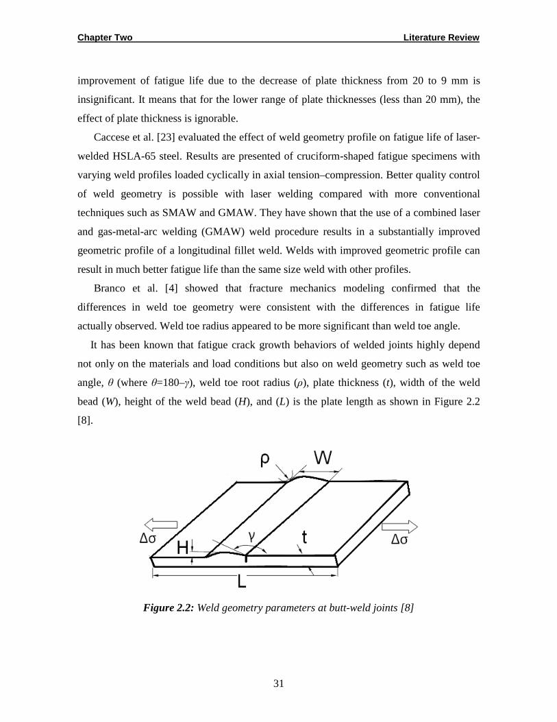
Chapter Two Literature Review
31
improvement of fatigue life due to the decrease of plate thickness from 20 to 9 mm is
insignificant. It means that for the lower range of plate thicknesses (less than 20 mm), the
effect of plate thickness is ignorable.
Caccese et al. [23] evaluated the effect of weld geometry profile on fatigue life of laser-
welded HSLA-65 steel. Results are presented of cruciform-shaped fatigue specimens with
varying weld profiles loaded cyclically in axial tension–compression. Better quality control
of weld geometry is possible with laser welding compared with more conventional
techniques such as SMAW and GMAW. They have shown that the use of a combined laser
and gas-metal-arc welding (GMAW) weld procedure results in a substantially improved
geometric profile of a longitudinal fillet weld. Welds with improved geometric profile can
result in much better fatigue life than the same size weld with other profiles.
Branco et al. [4] showed that fracture mechanics modeling confirmed that the
differences in weld toe geometry were consistent with the differences in fatigue life
actually observed. Weld toe radius appeared to be more significant than weld toe angle.
It has been known that fatigue crack growth behaviors of welded joints highly depend
not only on the materials and load conditions but also on weld geometry such as weld toe
angle, θ (where θ=180–γ), weld toe root radius (ρ), plate thickness (t), width of the weld
bead (W), height of the weld bead (H), and (L) is the plate length as shown in Figure 2.2
[8].
Figure 2.2: Weld geometry parameters at butt-weld joints [8]

Chapter Two Literature Review
32
Ferrica and Branco [48] investigated the effects of weld geometry factors on the fatigue
properties of cruciform and T-weld joints. The results showed that the ratio of thickness of
main plate and the radius of weld-toe (t/ρ) are the most important factors for the fatigue
properties of welded joints. As the thickness of plates is reduced, the fatigue strength and
life will increase in the case of T and cruciform joints. These results have been confirmed
by other researchers [51, 52] studied GMAW as welded butt welds in 25-30 mm AA5083-
O, AA5083-H116, AA5456-H116 and AA5456-H117 aluminum alloys. The investigations
concluded that the angle at the toe of the reinforcement is the most critical factor in the
determination of the fatigue life of as welded joints and actual maximum stress at the weld
toe.
The removal of weld reinforcement may increase the fatigue life, whether exposed to
air or seawater, if care is taken to prevent surface defects during the bead-removal process.
Niu and Glinka [53] derived an empirical relation, accounting for the stress concentration
Kt at weld toe, by FE methods [8, 28] as follows:
469.0
572.0512.01
+=ρ
θ tK t (2.4)
where θ is the weld toe corner (then θ =180 - γ) angle in radian, t is the plate thickness, and
ρ is the weld toe root radius (see Figure 2.2).
Figure 2.3 shows the stress concentration factor as a function of weld angle and
thickness for a weld toe radius equal 1 mm. It was shown that the stress near a notch tip is
dependent mainly on the stress concentration factor Kt, the notch tip radius, ρ, and the weld
toe corner angle θ. Therefore, it can be concluded that any changes in the weld toe radius
mostly affect the stress concentration factor Kt, and the stress field in the close vicinity of
the weld toe.

Chapter Two Literature Review
33
0
0.5
1
1.5
2
2.5
3
3.5
4
4.5
0 10 20 30 40t/ρ
Kt
θ=30 θ=45 θ=90
Figure 2.3: Stress concentration factor as a function of weld angle (radian) and thickness (mm) for weld toe radius equal to 1 mm
The welds with their reinforcement removed were more sensitive to porosity compared
with the weld with reinforcement intact, although the former gave longer life than as
welded joints when porosity level was lower. In other words, when a relatively higher level
of weld inner-defects such as porosity, inclusions, lack of fusion and LOP, exist in a
weldment, welds with bead reinforcement removed may exhibit shorter life than those of
welds with bead on. This situation could be fairly true for weldments with a high level of
weld inner-defects, for example weld repaired structures. Therefore, the as-welded joints
can exhibit different fatigue crack growth performance behavior compared to that of the
weld with bead reinforcement intact, depending on the situation.
Motarjemi et al. [54] studied for cruciform joints the effect of attachment thickness,
main plate thickness, weld leg length, and initial LOP size on fatigue life by integration of
the Paris’ law. For T-welded joints, the effect of different support span has also been
investigated. The results are reported as fatigue life curves for both types of joints. All the
curves show higher fatigue life for T-joints than for cruciform joints. The studied
parameters include the attachment and main plate thickness (B and T, respectively), weld
leg length (h), support span (D) (for the T joints only) and initial lack of root penetration
size (2ai). The details of the parameters covered in this study are shown in Figure 2.4.
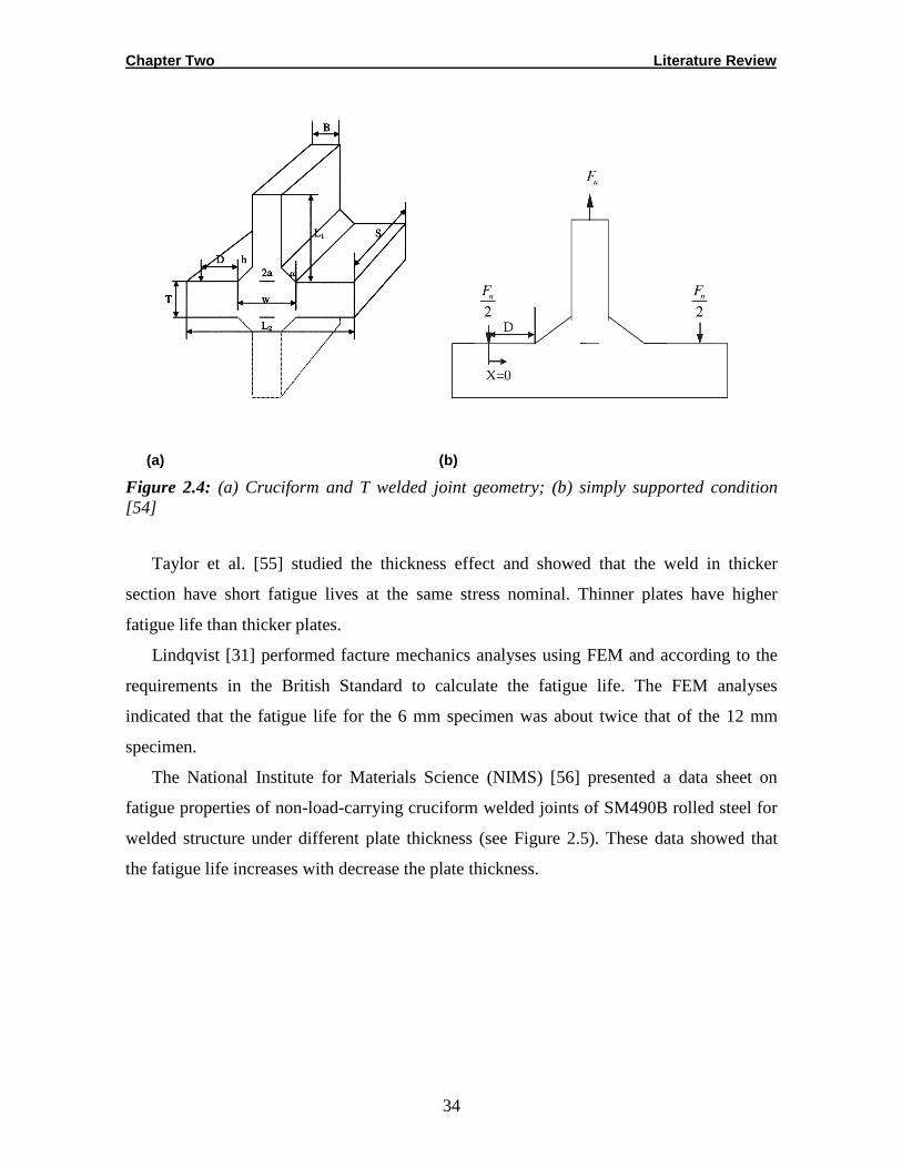
Chapter Two Literature Review
34
(a) (b)
Figure 2.4: (a) Cruciform and T welded joint geometry; (b) simply supported condition [54]
Taylor et al. [55] studied the thickness effect and showed that the weld in thicker
section have short fatigue lives at the same stress nominal. Thinner plates have higher
fatigue life than thicker plates.
Lindqvist [31] performed facture mechanics analyses using FEM and according to the
requirements in the British Standard to calculate the fatigue life. The FEM analyses
indicated that the fatigue life for the 6 mm specimen was about twice that of the 12 mm
specimen.
The National Institute for Materials Science (NIMS) [56] presented a data sheet on
fatigue properties of non-load-carrying cruciform welded joints of SM490B rolled steel for
welded structure under different plate thickness (see Figure 2.5). These data showed that
the fatigue life increases with decrease the plate thickness.
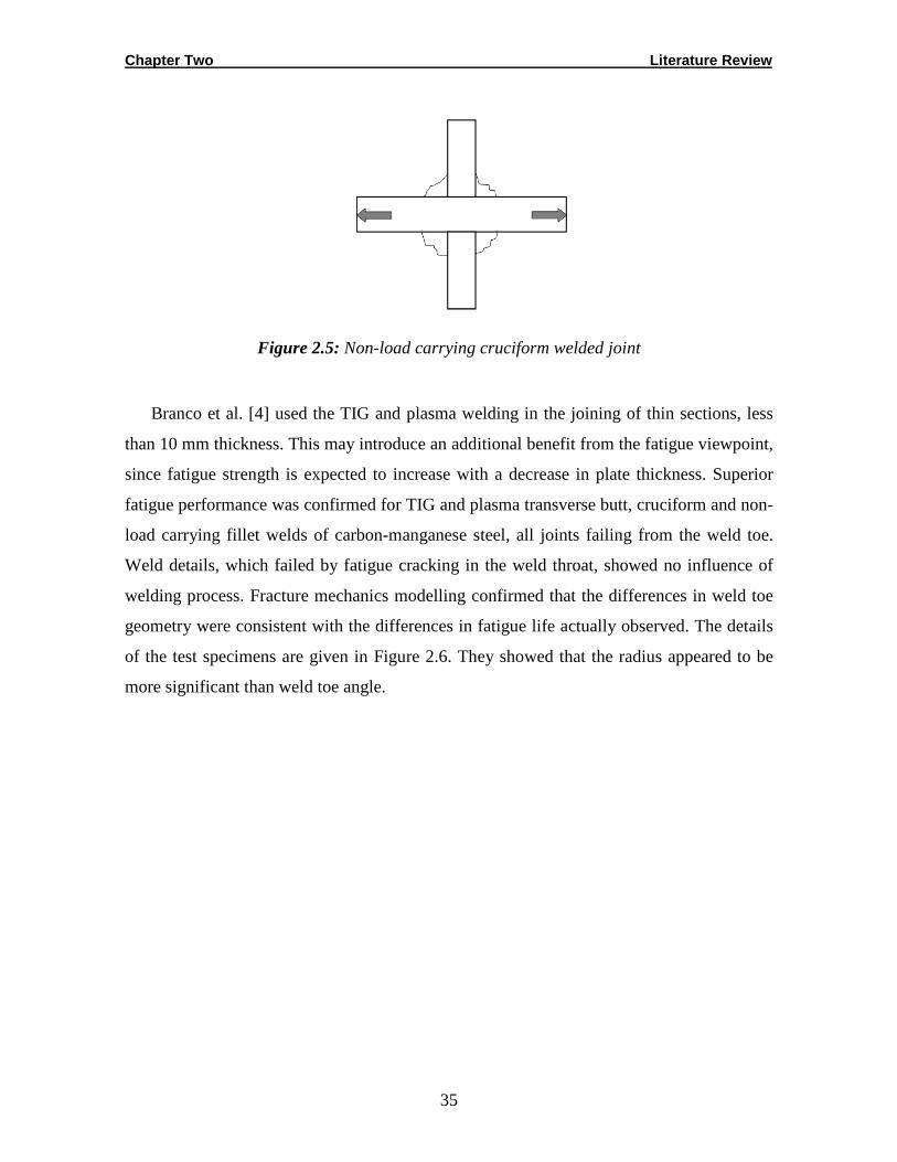
Chapter Two Literature Review
35
Figure 2.5: Non-load carrying cruciform welded joint
Branco et al. [4] used the TIG and plasma welding in the joining of thin sections, less
than 10 mm thickness. This may introduce an additional benefit from the fatigue viewpoint,
since fatigue strength is expected to increase with a decrease in plate thickness. Superior
fatigue performance was confirmed for TIG and plasma transverse butt, cruciform and non-
load carrying fillet welds of carbon-manganese steel, all joints failing from the weld toe.
Weld details, which failed by fatigue cracking in the weld throat, showed no influence of
welding process. Fracture mechanics modelling confirmed that the differences in weld toe
geometry were consistent with the differences in fatigue life actually observed. The details
of the test specimens are given in Figure 2.6. They showed that the radius appeared to be
more significant than weld toe angle.

Chapter Two Literature Review
36
(a)
(b)
(c)
Figure 2.6: Details of the tested welded joints: (a) butt welds from one side (TIG and plasma); (b) butt welds from both sides (MMA and 6mm TIG); (c) cruciform fillet welded specimens designed to fail in a plate at weld toe (non-load carrying attachments) and failing a weld throat (load carrying) [4]
2.6.2. Weld Defects and Metallurgy
Weld defects are those imperfections or discontinuities produced in the weldments
because of the weld process, such as porosity, LOP, slag inclusions, incomplete fusion,
misalignment, undercut, weld profile etc. These weld defects can significantly influence the
local stress field in the vicinity of welds when the welded component is subjected to cyclic
fatigue load. In most cases, weld defects lead to severe stress concentrations and thus
accelerate fatigue crack growth. Several works studied the effects of LOP on the fatigue
behavior of welds. They concluded that LOP defects can seriously reduce the fatigue life of
both types of weld, those with the reinforcement intact and those with the reinforcement
removed. They reported that the effects of internal discontinuities on fatigue performance
of welds with reinforcements are minimal. The effect of weld reinforcement is so marked
that only critical defects would affect the fatigue behavior and this is related to the loss of
cross section area. Porosity only becomes a factor when the reinforcement is removed.
Weld toe cracks are often found in many important welded structures. The ability to
assess the effects of these defects on fatigue life of the welded structures is therefore of
Chapter Two Literature Review
37
practical significance. To carry out this assessment, it is necessary to have reliable SIF
solutions.
2.6.3. Materials and Welding Techniques
Chemical composition and condition of welding materials, including base metal and
fillet material can directly affect fatigue crack growth rates of welded joints [57]. Different
materials have different mechanical properties and characteristics under cyclic loading.
Phase change will occur in most kinds of steels when subjected to the welding process and
residual stresses are introduced by these phase changes in areas like the weld toe and heat-
affected zone. Generally these residual stresses tend to be tensile stress on hot spots and
hence reduce the fatigue performance of welded joints.
The magnitude of this influence is dependent on the type of material. However, in the
case of austenite stainless steel and 5083 aluminum alloys, no phase change occurs and
hence no residual stresses due to phase change exist, although the latter may suffer
substantial strength loss due to heating during the weld process. Different welding
processes also have different effects on the fatigue properties of welded joints. Some
welding methods such as submerged arc welding cause heavy heat input in the weld joints,
producing higher thermal residual stresses. As mentioned previously, defects introduced
during the weld process such as undercut, lack of fusion, lack of penetration, misalignment,
porosity and poor profiles can also have a significant influence on the fatigue properties of
welded joints [8].
2.6.4. Weld Residual Stresses
Residual stresses are known since many years as one of the most critical factors which
can significantly influence the fatigue properties of welded joints. Many researchers have
reported on the basis of their experiments that the magnitude of the highest tensile residual
stress may approach the yield strength of the parent material in some critical locations of
weldments [5].
Previous investigations [24, 37] indicated that the WRS have also significant effects on
the fatigue crack initiation phase and the early stage of crack propagation.

Chapter Two Literature Review
38
2.7. Residual Stress Effects on Fatigue Life of Wel ded Joints
Residual stresses are stresses that remain in components after the applied external load
is removed. Residual stresses in engineering structures occur from welding and other
manufacturing processes such as rolling, forging and casting. These stresses have a
significant influence on the fatigue lives of structural components [5].
Weld residual stress (WRS) introduced by the welding process can come from the
expansion and shrinkage of weldments during heating and cooling [24], misalignment and
microstructure variation in weldments and heat-affected zone (HAZ). Residual stresses in
weldments have two effects. Firstly, they produce distortion, and second, they can be the
cause of premature failure especially in fatigue fracture under lower external cyclic loads
[8].
It has been confirmed that WRS is quite large and will be tensile in the vicinity of the
weld, where their magnitude is approximately equal to the yield strength of the weld metal,
as shown in Figure 2.7.
(a) (b)
(c)
Figure 2.7: Typical longitudinal WRS distribution at butt weld [28]: (a) mild steel; (b) aluminum alloy; (c) high alloyed structural steel [8]
Some researchers confirmed that the tensile residual stresses could significantly decrease
the fatigue properties of welded joints. It has been shown that tensile residual stresses in
Chapter Two Literature Review
39
welded structures can be as high as the yield strength of the material and have a detrimental
effect on the fatigue behaviour. On the other hand, compressive stresses on the surface of
weldments could have a favorable effect on fatigue life and they can significantly improve
the fatigue strength of welded structures [5, 9, 59].
Itoh et al. [58] studied the effect of residual stress on fatigue crack propagation rate in
longitudinal welded residual stress field and found that the effect of crack growth rate in a
weld residual stress field could be evaluated in terms of the effective stress intensity range,
based on the measurement of effective stress ratio and crack opening ratio. The effective
SIF and the effective stress ratio can be applied to predict the fatigue crack growth rate in
both tensile and compressive residual stress field by using base material’s crack growth rate
data with different stress ratios.
Other works investigated residual stresses on the crack initiation phase only such as
Teng et al. [24], who studied the effect of residual stresses on the fatigue crack initiation
(FCI) life in high cycle fatigue of butt welded joints. They found that the localized heating
caused by welding and subsequent rapid cooling can cause tensile residual stresses at the
weld toe of butt-welded joints. These tensile residual stresses were considered one of the
major influences on fatigue strength.
O’Dowd et al. [60] determined the SIF value for cracks of different sizes at the weld toe
due to the weld residual stress using the FEM. They also compared the SIFs for the stress
distributions provided in R6 and BS7910 and from neutron diffraction measurements along
the weld toe line which determines the stress field directly from the measured elastic strain
for three mutually perpendicular stress components (transverse, longitudinal and normal
stress), see Figure 2.8 The three stresses are obtained from three strain components using
Hook’s law. Very dense mesh has been used near the weld toe of the T-plate weld joint.
All calculations were carried out using the commercial FE software package, ABAQUS.
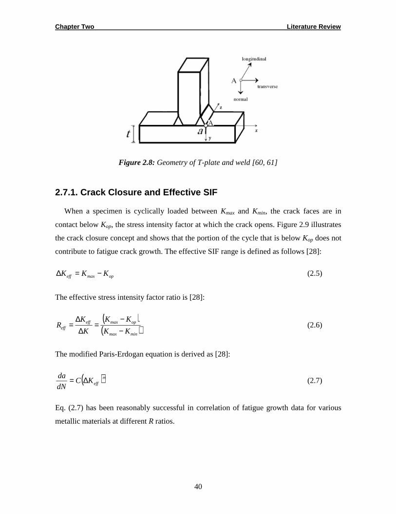
Chapter Two Literature Review
40
Figure 2.8: Geometry of T-plate and weld [60, 61]
2.7.1. Crack Closure and Effective SIF
When a specimen is cyclically loaded between Kmax and Kmin, the crack faces are in
contact below Kop, the stress intensity factor at which the crack opens. Figure 2.9 illustrates
the crack closure concept and shows that the portion of the cycle that is below Kop does not
contribute to fatigue crack growth. The effective SIF range is defined as follows [28]:
opmaxeff KKK −=∆ (2.5)
The effective stress intensity factor ratio is [28]:
( )( )minmax
opmaxeffeff KK
KK
K
KR
−−
=∆
∆= (2.6)
The modified Paris-Erdogan equation is derived as [28]:
( )meffKC
dN
da ∆= (2.7)
Eq. (2.7) has been reasonably successful in correlation of fatigue growth data for various
metallic materials at different R ratios.
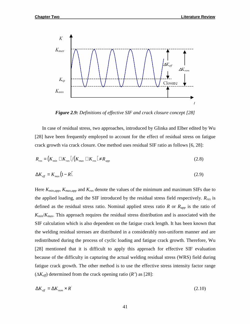
Chapter Two Literature Review
41
Figure 2.9: Definitions of effective SIF and crack closure concept [28]
In case of residual stress, two approaches, introduced by Glinka and Elber edited by Wu
[28] have been frequently employed to account for the effect of residual stress on fatigue
crack growth via crack closure. One method uses residual SIF ratio as follows [6, 28]:
( ) ( ) appresmaxresminres RKKKKR ≠++= (2.8)
( )RKK maxeff −=∆ 1 (2.9)
Here Kmin,app, Kmax,app and Kres denote the values of the minimum and maximum SIFs due to
the applied loading, and the SIF introduced by the residual stress field respectively. Rres is
defined as the residual stress ratio. Nominal applied stress ratio R or Rapp is the ratio of
Kmin/Kmax. This approach requires the residual stress distribution and is associated with the
SIF calculation which is also dependent on the fatigue crack length. It has been known that
the welding residual stresses are distributed in a considerably non-uniform manner and are
redistributed during the process of cyclic loading and fatigue crack growth. Therefore, Wu
[28] mentioned that it is difficult to apply this approach for effective SIF evaluation
because of the difficulty in capturing the actual welding residual stress (WRS) field during
fatigue crack growth. The other method is to use the effective stress intensity factor range
(∆Keff) determined from the crack opening ratio (R’) as [28]:
'RKK nomeff ×∆=∆ (2.10)
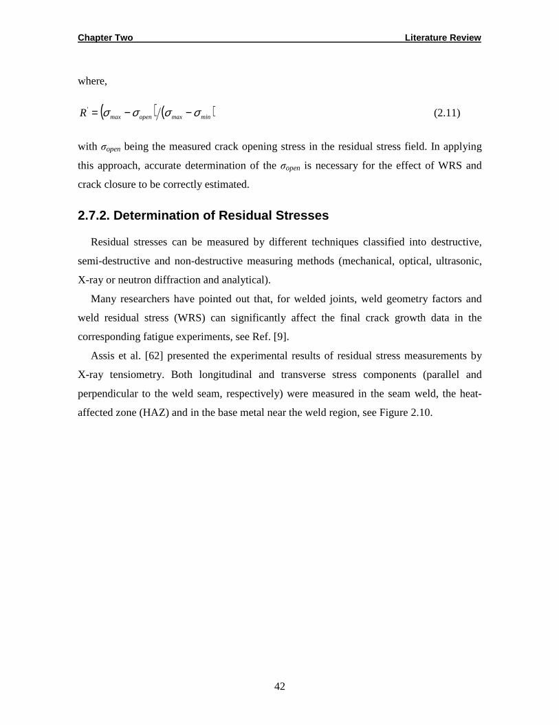
Chapter Two Literature Review
42
where,
( ) ( )minmaxopenmaxR σσσσ −−=' (2.11)
with σopen being the measured crack opening stress in the residual stress field. In applying
this approach, accurate determination of the σopen is necessary for the effect of WRS and
crack closure to be correctly estimated.
2.7.2. Determination of Residual Stresses
Residual stresses can be measured by different techniques classified into destructive,
semi-destructive and non-destructive measuring methods (mechanical, optical, ultrasonic,
X-ray or neutron diffraction and analytical).
Many researchers have pointed out that, for welded joints, weld geometry factors and
weld residual stress (WRS) can significantly affect the final crack growth data in the
corresponding fatigue experiments, see Ref. [9].
Assis et al. [62] presented the experimental results of residual stress measurements by
X-ray tensiometry. Both longitudinal and transverse stress components (parallel and
perpendicular to the weld seam, respectively) were measured in the seam weld, the heat-
affected zone (HAZ) and in the base metal near the weld region, see Figure 2.10.
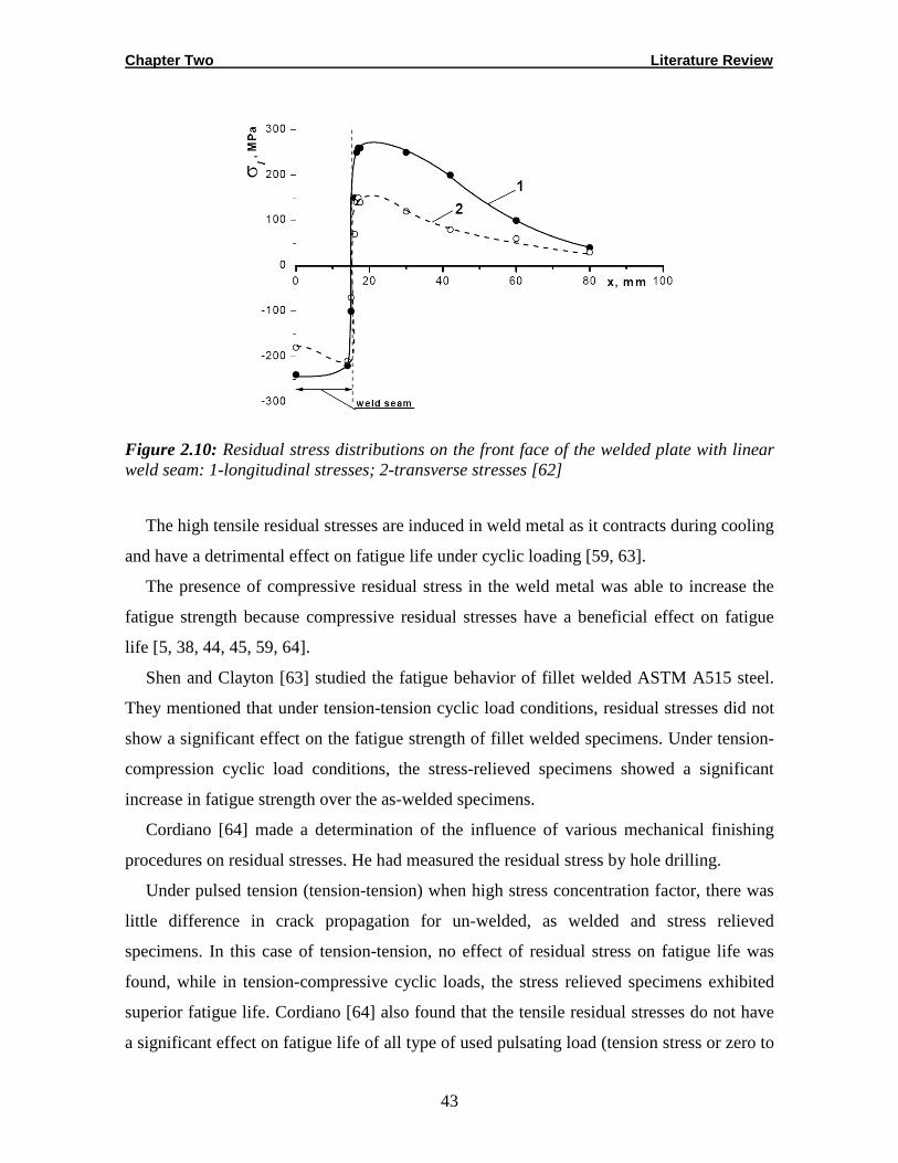
Chapter Two Literature Review
43
Figure 2.10: Residual stress distributions on the front face of the welded plate with linear weld seam: 1-longitudinal stresses; 2-transverse stresses [62]
The high tensile residual stresses are induced in weld metal as it contracts during cooling
and have a detrimental effect on fatigue life under cyclic loading [59, 63].
The presence of compressive residual stress in the weld metal was able to increase the
fatigue strength because compressive residual stresses have a beneficial effect on fatigue
life [5, 38, 44, 45, 59, 64].
Shen and Clayton [63] studied the fatigue behavior of fillet welded ASTM A515 steel.
They mentioned that under tension-tension cyclic load conditions, residual stresses did not
show a significant effect on the fatigue strength of fillet welded specimens. Under tension-
compression cyclic load conditions, the stress-relieved specimens showed a significant
increase in fatigue strength over the as-welded specimens.
Cordiano [64] made a determination of the influence of various mechanical finishing
procedures on residual stresses. He had measured the residual stress by hole drilling.
Under pulsed tension (tension-tension) when high stress concentration factor, there was
little difference in crack propagation for un-welded, as welded and stress relieved
specimens. In this case of tension-tension, no effect of residual stress on fatigue life was
found, while in tension-compressive cyclic loads, the stress relieved specimens exhibited
superior fatigue life. Cordiano [64] also found that the tensile residual stresses do not have
a significant effect on fatigue life of all type of used pulsating load (tension stress or zero to

Chapter Two Literature Review
44
maximum tension range). While under reversed cyclic load, the effect becomes apparent
and increases with decrease the stress range to some limit.
Nguyen et al. [37] studied the effect of residual stresses and weld geometry on the
fatigue life of butt welded joints by developing an analytical model using LEFM,
superposition and FE approaches. They aimed to find the theoretical explanations for the
improvement of fatigue life due to the compressive residual stresses introduced by various
post-weld surface treatments and improved weld geometry because of the theoretical
analysis of the effect of compressive residual stresses and weld geometry on the
improvement of fatigue life of welded structures is still not clear. The residual stress
distributions are not measured but assumed based on numbers of studies related to residual
stresses in as-welded and shot peened welded joints.
O’Dowd et al. [60] obtained the residual stresses in welded ferritic steel T-plates,
determined using neutron diffraction.
The measured data for the T-plate are shown in Figure 2.11. It has been found that the
transverse residual stress distribution for different plate sizes and yield strength are of
similar shape and magnitude when normalized appropriately and peak stresses are on the
order of the material yield strength. The magnitude of the peak transverse stress is about
450 MPa (approximately 60 percent of the material yield strength) and occurs at a distance,
y, about 5 mm from the weld toe (see Figure 2.11). SIFs corresponding to this residual
stress field due to a crack of varying size at the weld toe will be calculated and discussed in
Chapter 5 in relevant comparisons between the current work and the Refs. [60, 61].

Chapter Two Literature Review
45
(a) (b)
Figure 2.11: Residual stress distributions for the high strength steel T-plate, Grade SE702 [10]: (a) stress in MPa and (b) normalised stress [60, 61]
Servetti et al. [65] predicted fatigue crack growth rate in welded butt joints. They
presented a simple method for predicting fatigue crack growth (FCG) using base material
coupon test data and the effective stress ratio to account for the residual stress effect. FEM
was used for calculation the SIF due to the applied and residual stress field.
2.8. Superposition Method
A quantitative assessment of the influence of a residual stress field on failure can be
made by applying the principle of superposition to calculate an effective stress intensity
factor, Keff.
Stacey and Webster [66] quantified the influence of residual stress distributions on the
SIFs developed in thick-walled cylinders containing line cracks and they evaluated the SIF
caused by residual stress field, Kres using the superposition principle.
Nguyen, Wahab and Maksymowicz et al. [37, 67, 68] developed an analytical model
using LEFM, FEA, dimensional analysis and superposition approaches to determine the
effect of residual stresses, weld geometry and undercut on the fatigue life of butt welded
joints.
Ramesh [6] found that the effects of the compressive residual stresses obtained from
overloads and cold expansion of holes are included in the calculation of fatigue crack
propagation by using the superposition method. The superposition method can account for
Chapter Two Literature Review
46
residual stresses by a superposition of applied and residual SIFs, Kapp and Kres respectively,
to give the total SIFs, KT under mode-I conditions [6] i.e.:
resappT KKK += (2.12)
With the assumption that the applied cyclic stress does not significantly alter the state of
the residual stress during crack propagation, the total SIF range is [6]:
( ) ( ) ( ) ( )appappminappmax
resappminresappmaxTminTmaxT
KKK
KKKKKKK
∆=−=
+−+=−=∆
,,
,, (2.13)
and Rres is the residual SIF ratio as stated in Eq. (2.8).
The SIF range does not change since the SIF from the residual stress is negated, but the
residual SIFs have an effect on the stress ratio. Hence, fatigue crack growth is predicted
using the following correlation [6]:
),( resRKfdN
da ∆= (2.14)
2.8.1. Residual Stresses Distribution
Profiles for residual stresses are presented in structural integrity assessment procedures
for European industry (SINTAP). The aim of SINTAP document (Task 4) [69] is to
propose a single reference source for residual stress profiles taken from open literature and
SINTAP project. The profiles presented in SINTAP are more realistic than those proposed
in the recent codes (except BS 7910 [14]) but still conservative [69].
Lee et al. [70] carried out reviews of through thickness transverse residual stress
distribution measurements in a number of components, manufactured from a range of
steels. They considered the residual stresses introduced by welding and mechanical
deformation. The geometries consisted of welded T-plate joints, pipe butt joints, tube-on-
plate joints, tubular Y-joints and tubular T-joints as well as cold bent tubes and repair
welds.
Chapter Two Literature Review
47
Lee et al. [71] determined the residual stress distributions for plate T-butt welds from a
detailed FEA of the welding process and they were compared with those of the measured
data for validation. The residual stress distributions from the analyses and measurements
were shown to be in similar shape. The distributions were found to be below the master
curve (upper bound curve) for the residual stresses that were previously determined from a
statistical analysis for a range of weld geometries and materials. A failure assessment for
the T-butt weld with cracks under residual stress distributions has been carried out.
2.8.1.1. R6 Distributions for T-Plate
In the R6 procedure, two approaches for defining residual stress profiles in welded T-
plates are provided, depending on the available information about welding conditions [61].
If the welding conditions are known or can be estimated, then the residual stress profiles
will be given according to the size of the plastic zone (r0) [61]. If the welding conditions are
unknown, then BSI7910 polynomial distribution functions are provided (see Eq. 2.15).
More details are found elsewhere [61, 69].
2.8.1.2. Polynomial Distributions for T-Plate and B utt Welds
If weld informations is unavailable then the BS7910 polynomial distribution is used
[61]. BS7910 provides two transverse residual stress distributions for T-plate joints. The
first transverse residual stress distribution is a polynomial function representing an upper
bound fit to experimental data and is given by Eq. (2.15) as follows [69, 70]:
( ) ( ) ( ) ( )( )432 /087.21/485.42/125.24/3267.297.0/ tatatatay −+−+= σσ (2.15)
The transverse through thickness profile of butt welds is given as follows [69]:
( ) ( ) ( ) ( ) ( ) ( )( )65432 /36.96/16.244/45.215/115.83/533.14/917.01/ tatatatatatay −+−+−−= σσ (2.16)
This distribution is here referred to as BS7910 [107]. The second distribution follows
that in R6, with the distribution depending on the size of the plastic zone [61]. The distance
ro represents the size of the yielded zone (mm).
If ro ≤t, where t is the plate thickness (mm) as shown in Figure 2.8, then:
Chapter Two Literature Review
48
v
qkr
yo
ησ
= (2.17)
where k is a material constant that depends on the coefficients of thermal expansion,
Young’s modulus, density and specific heat of a material (Nmm/J), σy is yield or 0.2%
proof strength of the parent metal, q is arc power, v is weld travel speed and η is process
efficiency (fraction of arc power entering plate as heat). Typical values of k and η for a
range of materials are provided in the R6 documents. For ferritic steels the values provided
are k = 153 Nmm/J, and η= 0.8, more details are found in Ref. [61].
When the plastic zone size ro calculated by Eq. (2.17) is less than the base plate
thickness, the residual stress is taken to be that of the parent material yield stress level at the
weld toe, reducing linearly to zero over the size of the yielded zone as in R6. If Eq. (2.17)
results in a plastic zone greater than the base plate width, the stress is taken to be equal to
the yield strength across the whole specimen thickness [61].
This distribution as a function of the welding conditions and of the mechanical
properties of the materials was preferred because it is less conservative than the first one
(polynomial function from experimental measurements) [69].
The recommended transverse residual stress profile for the tubular T-joints is the same
polynomial function as that provided for T-plate welds (Eq. 2.15). Lee [61] mentioned that
the BS7910 provides a more conservative residual stress profile than R6 for the T-plate
while R6 is more conservative for the tubular T-joint.
2.8.2. Residual Stress Intensity Factor
Fracture assessment for cracks will generally require the linear elastic SIF due to the
weld residual stress and variation of weld geometry and any additional primary mechanical
loading.
It is well known that fatigue performance of a welded structure depends upon local
effects, such as local stress fields, defect conditions and material properties. Since the
defects of welded structures are in most cases so severe, the crack initiation phase can be
neglected.
Chapter Two Literature Review
49
LEFM principles can be used to evaluate the fatigue crack growth behavior and thus, to
predict fatigue life of welded structures. In order to appropriately assess fatigue crack
growth process in welded joints it is necessary to obtain accurate results for SIF solutions in
the crack propagation phase [8]. Generally the SIF for a crack in a welded joint depends on
the global geometry of the joint which includes the weld profile, crack geometry, residual
stress conditions and the type of loading. Therefore, the calculation of the SIF, even for
simple types of weldments, requires detailed analysis of the several geometric parameters
and loading systems. The two approaches that have mostly been used till now for assessing
SIFs for crack in weldments are weight function method and the FEM. The weight function
method is an analytical technique for deriving SIFs from knowledge of the stress
distribution in the un-cracked body. The numerical approach is based on basic weight
functions applied for SIF calculation:
∫=a
dxaxmxK0
),()(σ (2.18)
Usually in this equation, σ(x) is the stress distribution over the crack depth center line for
a body without cracks. The weight function m(x, a) is a unique property for a given body
geometry.
The stress distribution, σ(x) can be calculated by FE method. Weight functions m(x, a)
have been derived by Bueckner and Rice which are presented in Ref. [53] for 2-D and 3-D
model edge crack and surface semi-elliptical crack in finite thickness plate, respectively.
Equation (2.18) reflects the fact that when a crack slits over a highly-stressed area (i.e.,
σ(x) is high), the material ahead of the crack front will act as an alternative stress path, i.e. it
will be highly-stressed locally. The results from a 3-D analysis are shown in Figure 2.12
[1]. F(a) is shown for a plane plate and T-butt joint.
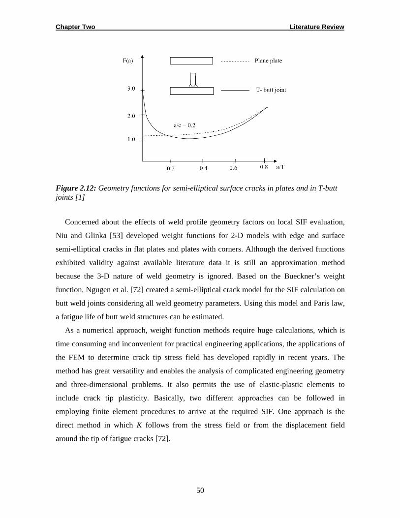
Chapter Two Literature Review
50
Figure 2.12: Geometry functions for semi-elliptical surface cracks in plates and in T-butt joints [1]
Concerned about the effects of weld profile geometry factors on local SIF evaluation,
Niu and Glinka [53] developed weight functions for 2-D models with edge and surface
semi-elliptical cracks in flat plates and plates with corners. Although the derived functions
exhibited validity against available literature data it is still an approximation method
because the 3-D nature of weld geometry is ignored. Based on the Bueckner’s weight
function, Ngugen et al. [72] created a semi-elliptical crack model for the SIF calculation on
butt weld joints considering all weld geometry parameters. Using this model and Paris law,
a fatigue life of butt weld structures can be estimated.
As a numerical approach, weight function methods require huge calculations, which is
time consuming and inconvenient for practical engineering applications, the applications of
the FEM to determine crack tip stress field has developed rapidly in recent years. The
method has great versatility and enables the analysis of complicated engineering geometry
and three-dimensional problems. It also permits the use of elastic-plastic elements to
include crack tip plasticity. Basically, two different approaches can be followed in
employing finite element procedures to arrive at the required SIF. One approach is the
direct method in which K follows from the stress field or from the displacement field
around the tip of fatigue cracks [72].
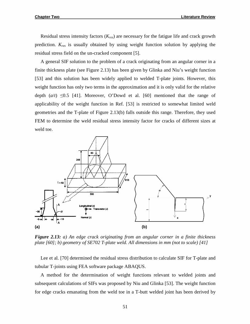
Chapter Two Literature Review
51
Residual stress intensity factors (Kres) are necessary for the fatigue life and crack growth
prediction. Kres is usually obtained by using weight function solution by applying the
residual stress field on the un-cracked component [5].
A general SIF solution to the problem of a crack originating from an angular corner in a
finite thickness plate (see Figure 2.13) has been given by Glinka and Niu’s weight function
[53] and this solution has been widely applied to welded T-plate joints. However, this
weight function has only two terms in the approximation and it is only valid for the relative
depth (a/t) ≤0.5 [41]. Moreover, O’Dowd et al. [60] mentioned that the range of
applicability of the weight function in Ref. [53] is restricted to somewhat limited weld
geometries and the T-plate of Figure 2.13(b) falls outside this range. Therefore, they used
FEM to determine the weld residual stress intensity factor for cracks of different sizes at
weld toe.
(a) (b)
Figure 2.13: a) An edge crack originating from an angular corner in a finite thickness plate [60]; b) geometry of SE702 T-plate weld. All dimensions in mm (not to scale) [41]
Lee et al. [70] determined the residual stress distribution to calculate SIF for T-plate and
tubular T-joints using FEA software package ABAQUS.
A method for the determination of weight functions relevant to welded joints and
subsequent calculations of SIFs was proposed by Niu and Glinka [53]. The weight function
for edge cracks emanating from the weld toe in a T-butt welded joint has been derived by
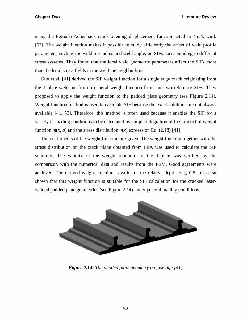
Chapter Two Literature Review
52
using the Petroski-Achenback crack opening displacement function cited in Niu’s work
[53]. The weight function makes it possible to study efficiently the effect of weld profile
parameters, such as the weld toe radius and weld angle, on SIFs corresponding to different
stress systems. They found that the local weld geometric parameters affect the SIFs more
than the local stress fields in the weld toe neighborhood.
Guo et al. [41] derived the SIF weight function for a single edge crack originating from
the T-plate weld toe from a general weight function form and two reference SIFs. They
proposed to apply the weight function to the padded plate geometry (see Figure 2.14).
Weight function method is used to calculate SIF because the exact solutions are not always
available [41, 53]. Therefore, this method is often used because it enables the SIF for a
variety of loading conditions to be calculated by simple integration of the product of weight
function m(x, a) and the stress distribution σ(x) expression Eq. (2.18) [41].
The coefficients of the weight function are given. The weight function together with the
stress distribution on the crack plane obtained from FEA was used to calculate the SIF
solutions. The validity of the weight function for the T-plate was verified by the
comparison with the numerical data and results from the FEM. Good agreements were
achieved. The derived weight function is valid for the relative depth a/t ≤ 0.8. It is also
shown that this weight function is suitable for the SIF calculation for the cracked laser-
welded padded plate geometries (see Figure 2.14) under general loading conditions.
Figure 2.14: The padded plate geometry on fuselage [41]
Chapter Two Literature Review
53
Applied SIF has been calculated from weight function given by Niu and Glinka.
However, this weight function is only valid for the relative depth a/t≤0.5. Therefore, Guo et
al. [41] presented widely applicable weight function solutions with a crack of relative depth
(a/t) up to 0.8 originating from the weld toe. They used the σ (x) distribution from FEA
[41].
More recently Glinka and Shen cited in Refs. [41, 73] have found that the following
general weight function expression can be used to approximate weight functions for a
variety of geometrical crack configurations subjected to one-dimensional mode-I stress
field [41]:
−+
−+
−+
−=
23
32
2/1
1 1111
12
2),(
a
xM
a
xM
a
xM
a
xa
axm
π (2.19)
where, a is the crack length and x the distance along the face of crack. Mi (i=1, 2, 3) are
parameters which depend only on the geometrical configuration of the cracked body.
In order to determine the weight function m(x, a) for a particular cracked body, it is
sufficient to determine the three parameters M1, M2, and M3 in expression (2.19). Because
the mathematical form of the weight function (2.19) is the same for all cracks, the same
method can be used for the determination of parameters M1, M2, and M3 and calculation of
SIFs from Eq. (2.18). The method of finding the Mi parameters was discussed in Ref. [41].
A variety of line load weight functions [72, 74] have been derived and published already.
The further details of the Mi determination were discussed in Ref. [41].
6.1)2(23
3
8.4)3(2
13
2
11
+−=
=−−=
YYM
M
YYM
u
u
π
π (2.20)
where,
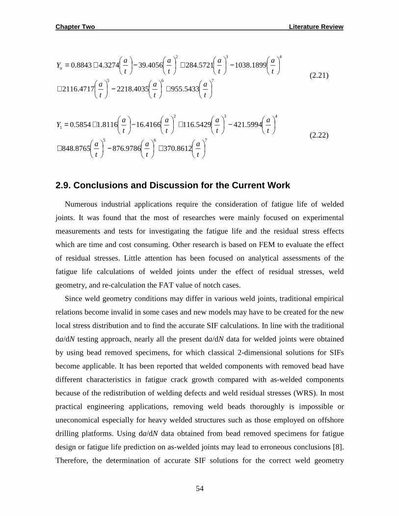
Chapter Two Literature Review
54
765
432
5433.9554035.22184717.2116
1899.10385721.2844056.393274.48843.0
+
−
+
−
+
−
+=
t
a
t
a
t
a
t
a
t
a
t
a
t
aYu
(2.21)
765
432
1
8612.3709786.8768765.848
5994.4215429.1164166.168116.15854.0
+
−
+
−
+
−
+=
t
a
t
a
t
a
t
a
t
a
t
a
t
aY
(2.22)
2.9. Conclusions and Discussion for the Current Wor k
Numerous industrial applications require the consideration of fatigue life of welded
joints. It was found that the most of researches were mainly focused on experimental
measurements and tests for investigating the fatigue life and the residual stress effects
which are time and cost consuming. Other research is based on FEM to evaluate the effect
of residual stresses. Little attention has been focused on analytical assessments of the
fatigue life calculations of welded joints under the effect of residual stresses, weld
geometry, and re-calculation the FAT value of notch cases.
Since weld geometry conditions may differ in various weld joints, traditional empirical
relations become invalid in some cases and new models may have to be created for the new
local stress distribution and to find the accurate SIF calculations. In line with the traditional
da/dN testing approach, nearly all the present da/dN data for welded joints were obtained
by using bead removed specimens, for which classical 2-dimensional solutions for SIFs
become applicable. It has been reported that welded components with removed bead have
different characteristics in fatigue crack growth compared with as-welded components
because of the redistribution of welding defects and weld residual stresses (WRS). In most
practical engineering applications, removing weld beads thoroughly is impossible or
uneconomical especially for heavy welded structures such as those employed on offshore
drilling platforms. Using da/dN data obtained from bead removed specimens for fatigue
design or fatigue life prediction on as-welded joints may lead to erroneous conclusions [8].
Therefore, the determination of accurate SIF solutions for the correct weld geometry

Chapter Two Literature Review
55
conditions is of practical significance for structural design and fatigue life evaluation of
welded structures as carried out in the current work.
Then, the assessment of fatigue life by fracture mechanics method is presented a useful
tool to avoid catastrophic failure of any structures and to provide FAT-data.
In spite of considerable fatigue design data which exist for welded joints in the
recommendations, the studies of the effects of crack growth parameters and initial crack
length are still not clear and have not been discussed enough.
Most researches have presented a limit of ranges for the initial crack length which will
affect fatigue life. Therefore, the current work presents the crack lengths and
recommendations to use an appropriate length of initial crack.
Different crack lengths were assumed, in addition the activity of the two types of cracks
(toe and LOP crack) are considered in some literature, i.e. independent crack growth at the
weld toe and weld root was assumed [15]. Then, the lowest FAT values were calculated. In
mind of the author, this consideration will conflict with the statistical nature of fracture.
This nature states that the normal crack in perpendicular direction to the load will
participate only in final failure effectively. Moreover, an initial crack length of 0.2 mm will
give a more conservative fatigue life.
In the current work, the gap distance was neglected between two plates to make
constancy in results for different geometries which are used. Some other literature used
different gap distances for some geometries and neglects for other, and this distance
according to the geometry was changed.
In the present work, the SIFs were calculated using the fracture analyses code 2-D
program (FRANC2D) due to limited available solutions of SIFs. FRANC2D simulator
provides reliable SIF solutions and is more familiar with mesh generation. No 3-D analysis
results in welded joints have yet been reported to the author’s knowledge.
From the available studies, the effects of weld residual stresses on the variation of
fatigue crack growth behavior still remains unclear. However, these effects are critical for
fatigue life evaluation of welded joints. In order to evaluate these effects on fatigue life of
welded joint structures, SIFs due to residual stresses have to be calculated accurately from
the product of weight function and residual stress distributions. In meanwhile, the effects of
Chapter Two Literature Review
56
different residual stress profiles and weld geometries on SIF and fatigue life still need to be
explained.
The superposition of Kres and Kapp (i.e., Kmax,app+Kres and Kmin,app+Kres) can be used.
However, such a superposition will change the resultant R ratio (Rres≠R) but the SIF ranges
(∆K) will remain the same (∆KT=∆Kapp). Therefore, it is needed to use the fatigue crack
growth equation which is sensitive to R like NASGRO equation or add the crack closure
phenomenon to the Paris’ model or any other model accounting for the state of affairs at the
crack tip. Research to date uses the modified Paris’ or Forman’ law and incorporates them
with residual SIF and total SIF to calculate lives which consider only the linear region of
crack growth curve. Little studies deal with NASGRO equation to incorporate residual
stress effects.
Most studies use the residual stresses measured by neutron diffraction or those
calculated from the FEM to calculate the Kres.
In mind of the author, up to date no studies were carried out on the numerical calculation
of Kres for each crack step using the weight function and residual stress distributions that
are issued in standards.
According to the above mentioned conclusions there are lacks in some points which will
be discussed in the current work. Therefore, the one aim of this thesis is to calculate the
entire crack growth rate with more analytical approach using weight function, polynomial
residual stress distributions and calculated initial crack length together with applied SIFs
which are calculated firstly from FRANC2D.
Therefore, the following models are used in calculations of the fatigue life. All models
have a theoretically-based calculation of the SIF from FE-FRANC2D program as follows:
1. Model-A : Numerical integration of Paris’ law using IIW-characteristic parameters (C,
and m). Then, the backward calculation by manipulating the initial crack length was carried
out to select the appropriate initial crack length, in turn to determine the FAT values. In this
model and due to linear relation between load and SIF, the calculating SIF was scaled with
different loads. By using the manipulated ai, the S-N curves and FAT can be obtained for
any new geometry.
Chapter Two Literature Review
57
2. Model-B : Numerical integration of NASGRO equation. The effect of stress ratio, R,
without the residual stresses were studied using the crack parameters which were calculated
from Model-A.
3. Model-C : Using Model-B with the effect of residual stresses. Therefore, the residual
stress ratio, residual stress distribution and the residual SIF have to be calculated in this
case. The latter was calculated from the product of the residual stresses distribution and the
weight function. In turn, different residual stress distributions can be used.
According to the current approaches the new FAT under the effects of geometries and
residual stresses can be calculated.
Chapter Three Modeling of Welded Joints and SIF Calculation
58
Chapter Three
MODELING OF WELDED JOINTS AND SIF
CALCULATION
3.1. Introduction
The stress intensity factor range (SIF) is the inevitable parameter, which must be
studied and calculated in fracture mechanics methods. The stress intensity factor, SIF
describes the fatigue action at a crack tip in terms of crack propagation. In this work,
SIFs have been calculated using fracture analysis code 2-dimensional program,
FRANC2D [46].
In welded joints, stress concentrations occur at the weld toe and at the weld root
which make these regions the points from which fatigue cracks may initiate [19]. These
cracks have been considered in the verification processes using FRANC2D software in
this chapter.
Calculating the fatigue life of welded structures and analyzing the progress of these
cracks using fracture mechanics technique requires an accurate calculation of the SIF.
The existing SIFs were usually derived for one particular geometry and type of loading.
In this study, the finite element method FEM (FRANC2D) was used to calculate the
SIF during crack propagation steps. It is verified to be highly accurate, with the
direction of crack propagation being predicted by using the maximum normal stress
criterion. A developed analytical approach for toe cracks in cruciform welded joints has
been used. On the other hand, in case of lack of penetration (LOP) a classical equation
from Frank and Fisher [21] is used. The calculated SIF results for some notch cases
have been verified with available solutions from International Institute of Welding
(IIW) [3, 34], British Standards Institution (BSI) [14, 75, 76] and literature.
A fairly good correlation was obtained and the results have confirmed the use of
FRANC2D to simulate different weld geometries. The results are shown and the
agreements are pretty good.
Chapter Three Modeling of Welded Joints and SIF Calculation
59
3.2. Two Dimensional Analysis of Welded Joints
This chapter describes the 2-dimensional analysis of welded joints using a FE
program (FRANC2D). The program was developed by the Cornell Fracture Group from
Cornell University, USA [46].
The objectives of this chapter are as follows:
1. Describing the details of welded joint analyses using FE program.
2. Presenting the possibility of two dimensional models to obtain accurate SIF
solutions.
3. Validation of the models by studying the effect of mesh size, mesh type and effect
of crack increment on SIF values.
4. Studying the effects of joints’ geometrical parameters on SIFs.
5. Validation with available solutions from literature (bench marking).
6. Using the validated model to find the SIF for new geometries with insurance of
accuracy.
In the application of fracture mechanics to fatigue problems, accurate determinations
of the SIF solutions for the case under analysis in the crack propagation phase are
needed in order to use the Paris’ equation in next steps to calculate the fatigue life.
Table 3.1 shows the cross-section of some welded joints used in this work.
Discarding major weld defects, fatigue cracks will originate from the weld toe, and then
propagate through the base material, or from the weld root, and then propagate through
the weld throat. More details are presented by Hobbacher [3, 32, 34].

Chapter Three Modeling of Welded Joints and SIF Calculation
60
Table 3.1: Fatigue cracking of some welded joints that used in this work
Transverse loaded butt weld (X-groove or V-groove) with
edges machined or ground flush to plate.
Double side complete weld penetration. Toe crack.
Transverse butt weld with weld reinforcement. Double side
complete penetration. Toe crack.
Transverse partial penetration butt welds, lack of penetration
(LOP) considered to be as a root crack.
Double side incomplete weld penetration.
Cruciform joint or T-joint, fillet welds or partial penetration K-
butt welds, toe and root crack.
Load can also be applied at the end of attached plate or main
plate, in y-, or in x-direction, respectively, in case of weld root
or weld toe crack consideration, respectively. θ is the weld toe
angle, a is the crack length, T is the main plate thickness.
Cruciform joint or T-joint, K-butt welds, full penetration, toe
crack.
Load can be applied at the end of attached plate in y-direction.
Weld toe crack will be considered in this case.
Usually toe cracks have been considered because they are easier to be observed with
the naked eye as well as with dye penetration tests and they are often found in many
important engineering welded structures. Moreover, there is a high stress concentration
located at this point [31, 32].
Chapter Three Modeling of Welded Joints and SIF Calculation
61
Shen and Clayton [63] stated that all the cracks were found to be initiated at the weld
end toe, in the location of the maximum stress concentration site. SIFs for these cracks
have to be determined.
For fracture mechanics treatments, in spite of the fact that several SIF handbooks
have been published, it is still difficult to find solutions adequate to many welded
configurations [41, 53]. This is mainly due to a wide variety of complex welded
geometries and loading systems.
It is known that the SIF for a crack in welded joints depends on the overall geometry
of the joint, the weld profile and the type of loading. Thus, the derivation of SIF even
for one type of weldment such as a T-butt, cruciform and butt joint requires detailed
analysis of several parameters such as plate thickness, weld thickness, weld angle, weld
toe radius and loading system.
By characterizing stable macroscopic crack growth using ∆K, it is possible to predict
the crack growth rate of a weld under cyclic loading, and hence the number of cycles
necessary for a crack to extend from some initial size, i.e., the size of pre-existing crack
or crack-like defects, to a maximum permissible size just before catastrophic failures
[77].
3.3. Finite Element Analysis
The analysis was undertaken based on the assumption of an initially isotropic elastic
material for both the base and its weld metal, in which a crack was subsequently
allowed to form and grow according to a fracture criterion. The advantage of symmetry
was considered to model quarter or half of the complete geometry.
The FRANC2D is a FE-based simulator for curvilinear crack propagation in planar
structures (plane stress, plane strain, and axisymmetric structures). CASCA which is
used for the creation the meshes, is a preprocessor for generating initial input files for
FRANC2D. FRANC2D program has the ability to analyze a cracked body using special
iso-parametric crack tip elements to describe the singularity ahead of the crack tip.
3.4. Mesh Description and Boundary Conditions
Figure 3.1 shows one type of the FE meshes used in the present study, which
comprises 8-nodded quadrilateral elements. Also the boundary conditions for T-joint or
cruciform joint and for butt joints are shown.
Chapter Three Modeling of Welded Joints and SIF Calculation
62
One side of the models was supported in the x-direction or y-direction and a uniform
stress distribution was applied at the other side along x-axis or y-axis, respectively. To
prevent the model from performing rigid body motions and rotation, one node on the
side where the model is supported in the x-direction or y-direction, is also locked in the
y-direction or x-direction, respectively, as shown in Figure 3.1.

Chapter Three Modeling of Welded Joints and SIF Calculation
63
(a)
(b)
(c)
(d)
Figure 3.1: Mesh configurations: (a) quarter cruciform model; (b) half cruciform model; (c) complete butt model; (d) half butt model
3.5. Material Properties
The material used in this study for the base material and weld metal was an extra
high strength hot rolled steel with the minimum yield strength 550 MPa and the tensile
strength minimum 600 MPa and maximum 760 MPa, respectively [31]. Fatigue testing
was calculated for an applied loading such that the maximum stress was maintained
x x x x x x x x x x
x x x x
y y y y y y y y y x, y
x, y
x x x x
x, y
x x x x
Chapter Three Modeling of Welded Joints and SIF Calculation
64
constant at 200 MPa and 104 MPa for cruciform and butt weld joints, respectively,
which fail from the weld toe.
It has to be emphasized in this part, that the input load is distributed with a constant
value in tensile direction. Keep in mind that this input load was as force per unit cross
section, i.e., in MPa.
Values of Poisson’s ratio υ and the modulus of elasticity E were chosen as 0.293 and
210 GPa, respectively.
Experimentally, many structures are optimized by the choice of high strength steel.
The reason for this choice is to allow higher stresses and to reduce dimensions taking
benefit of the high strength material with respect to the yield criterion. In fracture
mechanics, the fatigue strength of a welded joint is not primarily governed by the
strength of the base material of the joining members. Hence, the governing parameters
in fracture mechanics are mainly the local and global geometry of the joint, i.e., fatigue
strength is known to be closely related to the precise geometrical discontinuity of the
welded joint [77]. Therefore, the similar material as a single joint between the weld
metal and a base metal has been assumed in the simulation. The same steel was used in
case of LOP in load-carrying and non-load carrying cruciform and butt joints which fail
from LOP with a uniform tensile stress range of 96 MPa and 104 MPa, respectively.
In the absence of specified or measured material parameters, the values given below
are recommended to use with fatigue life calculation as characteristic values, Cchar=3e-
13, and m=3 for steel (units in Nmm-3/2 and mm).
3.6. Solution Procedure
The determination of the SIF for the 2-dimensional cruciform and butt welded joints
has been carried out using LEFM analysis. This method is well encoded in automatic
crack propagation in FE analyses FRANC2D. In general, the behavior of crack path
propagation (CP) in FRANC2D is almost the same as compared with available
experimental results. For every crack length, the values of the SIF were calculated
during crack propagation steps by FRANC2D program with suitable boundary
conditions, loading, crack growth criteria, and crack direction criteria.
In the following the FE analysis using FRANC2D is described.

Chapter Three Modeling of Welded Joints and SIF Calculation
65
3.6.1. Mesh Generation
A mesh generating program CASCA, which is distributed with FRANC2D, was used
to create the initial mesh configuration for FRANC2D simulations. Other mesh
generating programs can also be used, provided that a translator is available to convert
the mesh description to the FRANC2D *.inp format [78, 79]. The procedure for creating
a mesh is straightforward, as illustrated in Figure 3.2. To begin with, the problem
outline is first created, followed by the division of sub-regions within the problem
boundary in Figure 3.2(a). Prior to assigning the type of elements to each of the sub-
regions, the boundaries for all sub-regions are divided into the required number of
segments, Figure 3.2(b). The resulting mesh for the present simulation is shown in
Figure 3.2(c).
(a) (b)
(c)
Figure 3.2: Mesh generating procedure for cruciform joint, (CASCA program) [46]: (a) geometry with subdivided areas; (b) subdivided areas into segments; (c) generated mesh
Only one quarter of a cruciform specimen is modeled in FE analysis due to
symmetry. The material is assumed to be isotropic linear elastic.
3.6.2. Selection of Material Model
A linear elastic material model coupled to a linear elastic discrete fracture model was
used in the analysis. For this analysis and based on fracture mechanics for which linear
elastic fracture theory is considered reasonable, it was decided to restrict the analysis of
Chapter Three Modeling of Welded Joints and SIF Calculation
66
SIF solutions to the linear material behavior. The material assumed to be isotropic linear
elastic for base and weld metal.
3.6.3. Crack Propagation
A crack could propagate both from the weld toe and from the root. All calculations
of the present work were made on cracks propagating from either the toe or from the
weld root separately.
In order to study the capability of the program to simulate crack growth, an initial
non-cohesive edge crack was placed at the weld toe of the cruciform and butt weld
joints of the weld-base material interface, where it was predicted that critical tensile
stresses would occur.
The existence of crack-like imperfections and LOP in the welded joint is normally
considered to eliminate the so-called crack initiation stage of fatigue life. Therefore,
most of fatigue assessment of welded joints is concentrated on the crack growth stage of
the fatigue life. Having specified the location of the crack, the code was able to predict
the direction in which the crack would propagate. Prior to performing the analysis, it
was necessary to specify the magnitude of crack increment (∆a) and the number of steps
over which the crack would propagate. In the present study, a crack increment of 0.5
mm was chosen for all cases. However, this value could be changed according to
stability of fatigue life’s numerical integration (shown in next chapter). The crack
growth was simulated over 10 steps of increment depending on the plate thickness.
Moreover, in this study, the crack path was not pre-selected, but crack direction was
allowed to change according to the maximum tangential stress criterion [77]. Moreover,
the auto-mesh function was carried out automatically.
3.6.4. Modeling Procedures
For every crack length, the values of the SIF factor were calculated during crack
propagation steps by FRANC2D program with suitable boundary conditions, loading,
crack growth criteria, and crack direction criteria. The results were used to determine
the SIF as a function of crack length (a) for a particular case. Then, this function was
used to calculate the fatigue life using numerical integration of Paris’ equation (see
Chapter 4).
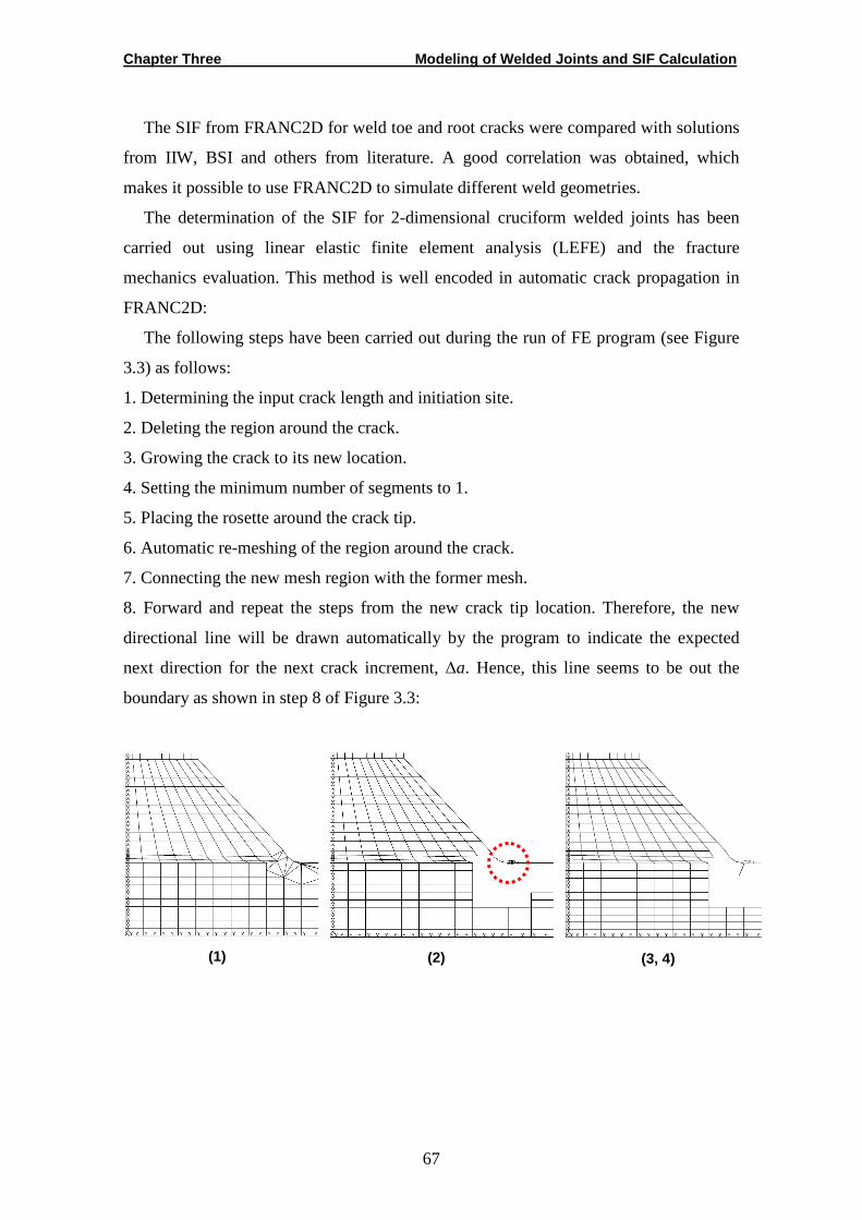
Chapter Three Modeling of Welded Joints and SIF Calculation
67
The SIF from FRANC2D for weld toe and root cracks were compared with solutions
from IIW, BSI and others from literature. A good correlation was obtained, which
makes it possible to use FRANC2D to simulate different weld geometries.
The determination of the SIF for 2-dimensional cruciform welded joints has been
carried out using linear elastic finite element analysis (LEFE) and the fracture
mechanics evaluation. This method is well encoded in automatic crack propagation in
FRANC2D:
The following steps have been carried out during the run of FE program (see Figure
3.3) as follows:
1. Determining the input crack length and initiation site.
2. Deleting the region around the crack.
3. Growing the crack to its new location.
4. Setting the minimum number of segments to 1.
5. Placing the rosette around the crack tip.
6. Automatic re-meshing of the region around the crack.
7. Connecting the new mesh region with the former mesh.
8. Forward and repeat the steps from the new crack tip location. Therefore, the new
directional line will be drawn automatically by the program to indicate the expected
next direction for the next crack increment, ∆a. Hence, this line seems to be out the
boundary as shown in step 8 of Figure 3.3:
(1) (2) (3, 4)
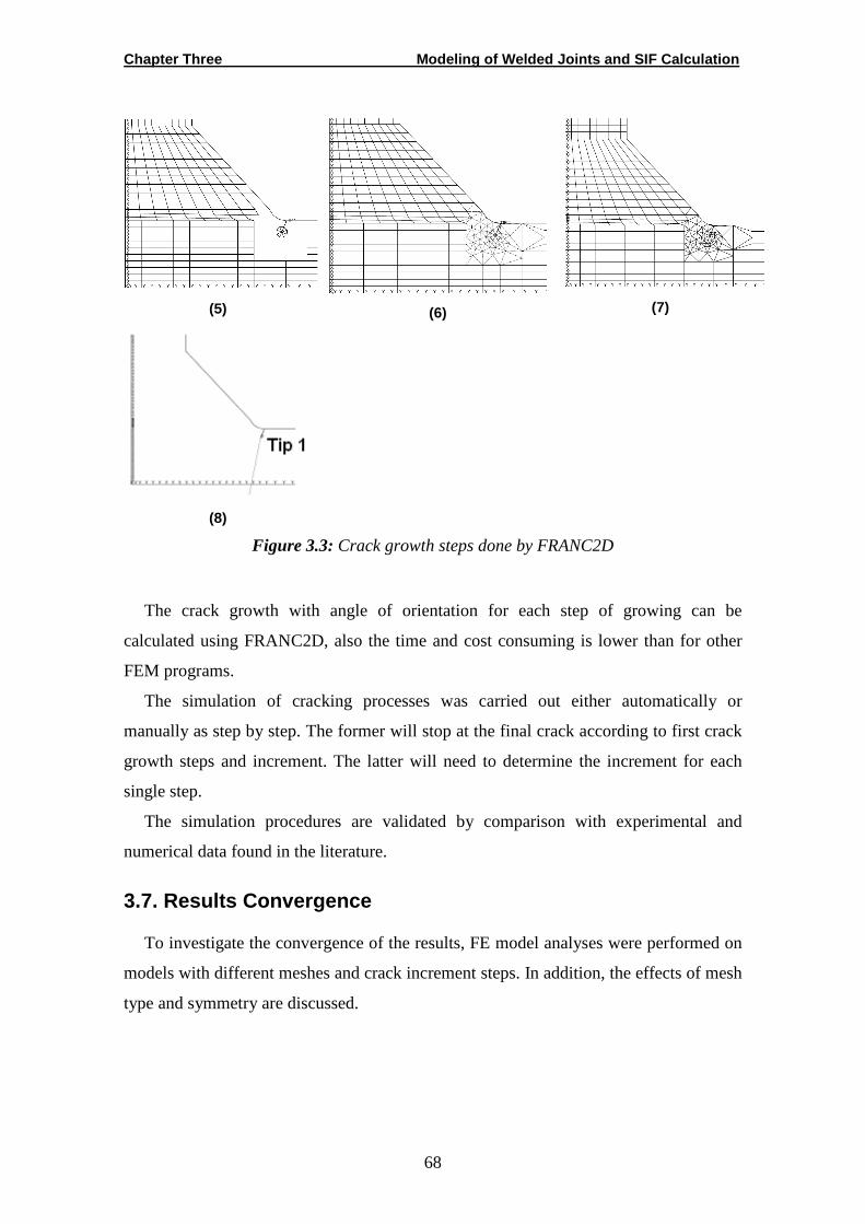
Chapter Three Modeling of Welded Joints and SIF Calculation
68
(5)
(6) (7)
(8)
Figure 3.3: Crack growth steps done by FRANC2D
The crack growth with angle of orientation for each step of growing can be
calculated using FRANC2D, also the time and cost consuming is lower than for other
FEM programs.
The simulation of cracking processes was carried out either automatically or
manually as step by step. The former will stop at the final crack according to first crack
growth steps and increment. The latter will need to determine the increment for each
single step.
The simulation procedures are validated by comparison with experimental and
numerical data found in the literature.
3.7. Results Convergence
To investigate the convergence of the results, FE model analyses were performed on
models with different meshes and crack increment steps. In addition, the effects of mesh
type and symmetry are discussed.
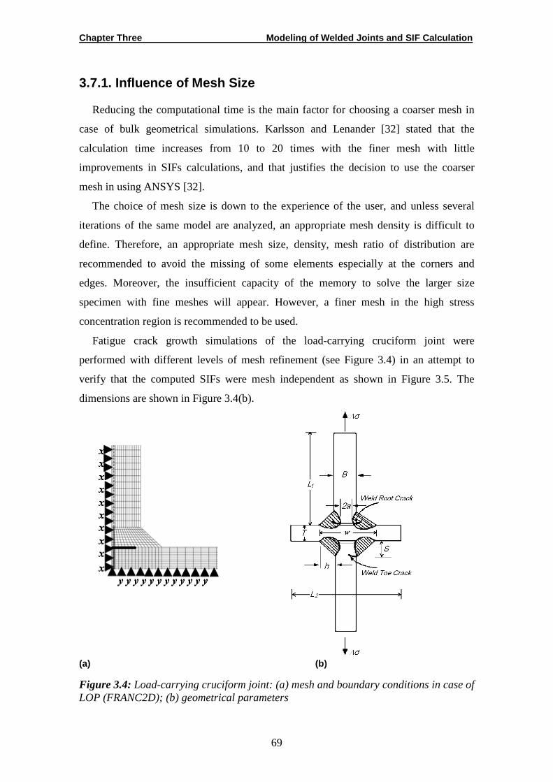
Chapter Three Modeling of Welded Joints and SIF Calculation
69
3.7.1. Influence of Mesh Size
Reducing the computational time is the main factor for choosing a coarser mesh in
case of bulk geometrical simulations. Karlsson and Lenander [32] stated that the
calculation time increases from 10 to 20 times with the finer mesh with little
improvements in SIFs calculations, and that justifies the decision to use the coarser
mesh in using ANSYS [32].
The choice of mesh size is down to the experience of the user, and unless several
iterations of the same model are analyzed, an appropriate mesh density is difficult to
define. Therefore, an appropriate mesh size, density, mesh ratio of distribution are
recommended to avoid the missing of some elements especially at the corners and
edges. Moreover, the insufficient capacity of the memory to solve the larger size
specimen with fine meshes will appear. However, a finer mesh in the high stress
concentration region is recommended to be used.
Fatigue crack growth simulations of the load-carrying cruciform joint were
performed with different levels of mesh refinement (see Figure 3.4) in an attempt to
verify that the computed SIFs were mesh independent as shown in Figure 3.5. The
dimensions are shown in Figure 3.4(b).
(a) (b)
Figure 3.4: Load-carrying cruciform joint: (a) mesh and boundary conditions in case of LOP (FRANC2D); (b) geometrical parameters
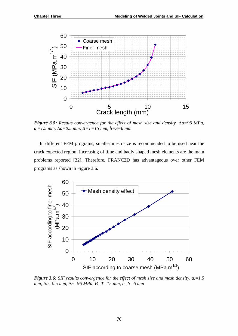
Chapter Three Modeling of Welded Joints and SIF Calculation
70
0
10
20
30
40
50
60
0 5 10 15Crack length (mm)
SIF
(M
Pa.
m1/
2 )
Coarse meshFiner mesh
Figure 3.5: Results convergence for the effect of mesh size and density. ∆σ=96 MPa, ai=1.5 mm, ∆a=0.5 mm, B=T=15 mm, h=S=6 mm
In different FEM programs, smaller mesh size is recommended to be used near the
crack expected region. Increasing of time and badly shaped mesh elements are the main
problems reported [32]. Therefore, FRANC2D has advantageous over other FEM
programs as shown in Figure 3.6.
0
10
20
30
40
50
60
0 10 20 30 40 50 60SIF according to coarse mesh (MPa.m1/2)
SIF
acc
ordi
ng to
fine
r m
esh
(MP
a.m
1/2 )
Mesh density effect
Figure 3.6: SIF results convergence for the effect of mesh size and mesh density. ai=1.5 mm, ∆a=0.5 mm, ∆σ=96 MPa, B=T=15 mm, h=S=6 mm
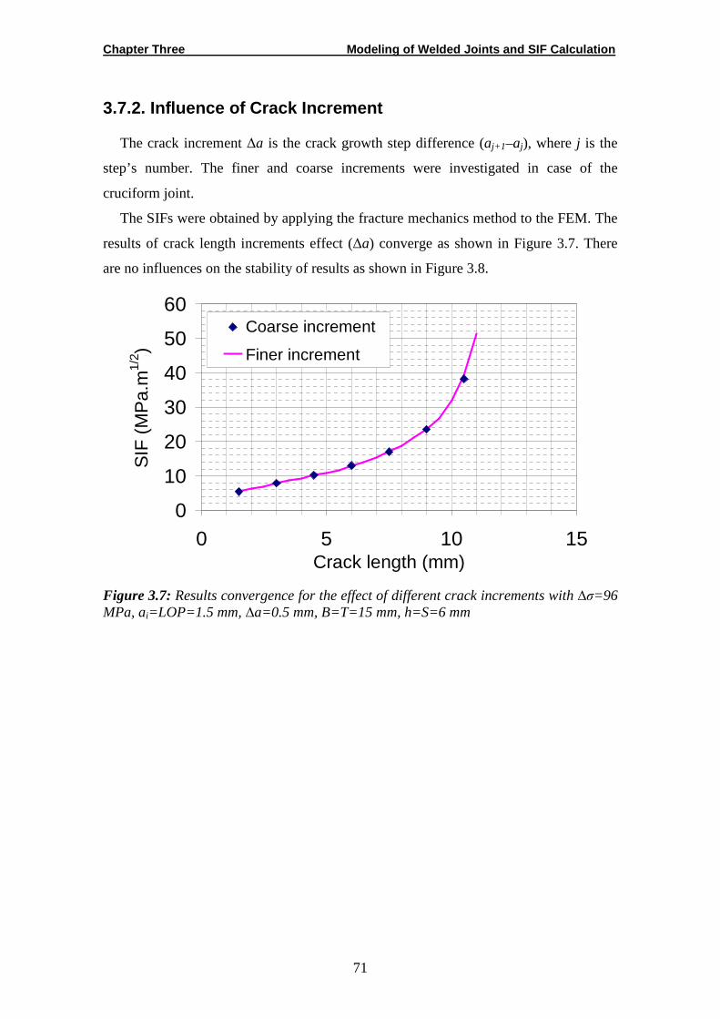
Chapter Three Modeling of Welded Joints and SIF Calculation
71
3.7.2. Influence of Crack Increment
The crack increment ∆a is the crack growth step difference (aj+1–aj), where j is the
step’s number. The finer and coarse increments were investigated in case of the
cruciform joint.
The SIFs were obtained by applying the fracture mechanics method to the FEM. The
results of crack length increments effect (∆a) converge as shown in Figure 3.7. There
are no influences on the stability of results as shown in Figure 3.8.
0
10
20
30
40
50
60
0 5 10 15Crack length (mm)
SIF
(M
Pa.
m1/
2 )
Coarse increment
Finer increment
Figure 3.7: Results convergence for the effect of different crack increments with ∆σ=96 MPa, ai=LOP=1.5 mm, ∆a=0.5 mm, B=T=15 mm, h=S=6 mm
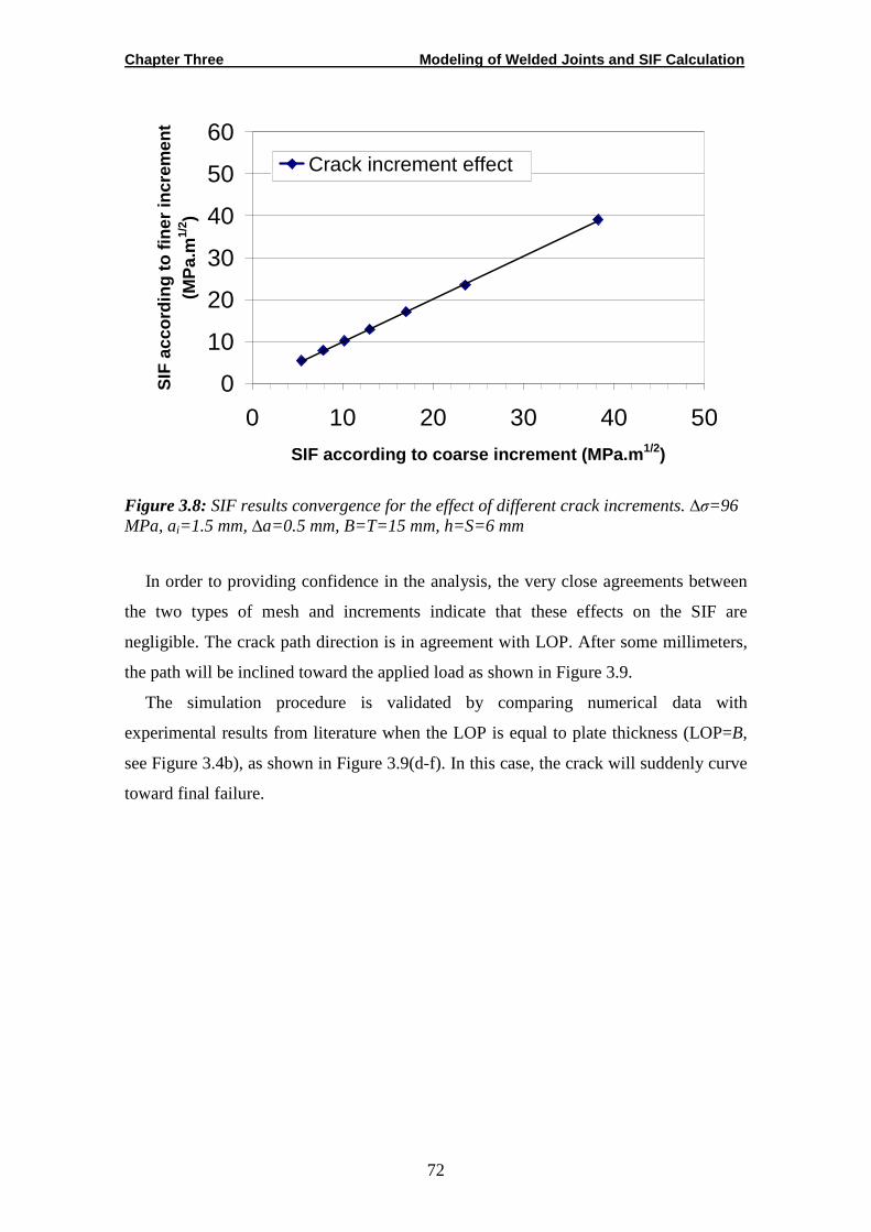
Chapter Three Modeling of Welded Joints and SIF Calculation
72
0
10
20
30
40
50
60
0 10 20 30 40 50
SIF according to coarse increment (MPa.m 1/2)
SIF
acc
ordi
ng to
fine
r in
crem
ent
(MP
a.m
1/2 )
Crack increment effect
Figure 3.8: SIF results convergence for the effect of different crack increments. ∆σ=96 MPa, ai=1.5 mm, ∆a=0.5 mm, B=T=15 mm, h=S=6 mm
In order to providing confidence in the analysis, the very close agreements between
the two types of mesh and increments indicate that these effects on the SIF are
negligible. The crack path direction is in agreement with LOP. After some millimeters,
the path will be inclined toward the applied load as shown in Figure 3.9.
The simulation procedure is validated by comparing numerical data with
experimental results from literature when the LOP is equal to plate thickness (LOP=B,
see Figure 3.4b), as shown in Figure 3.9(d-f). In this case, the crack will suddenly curve
toward final failure.
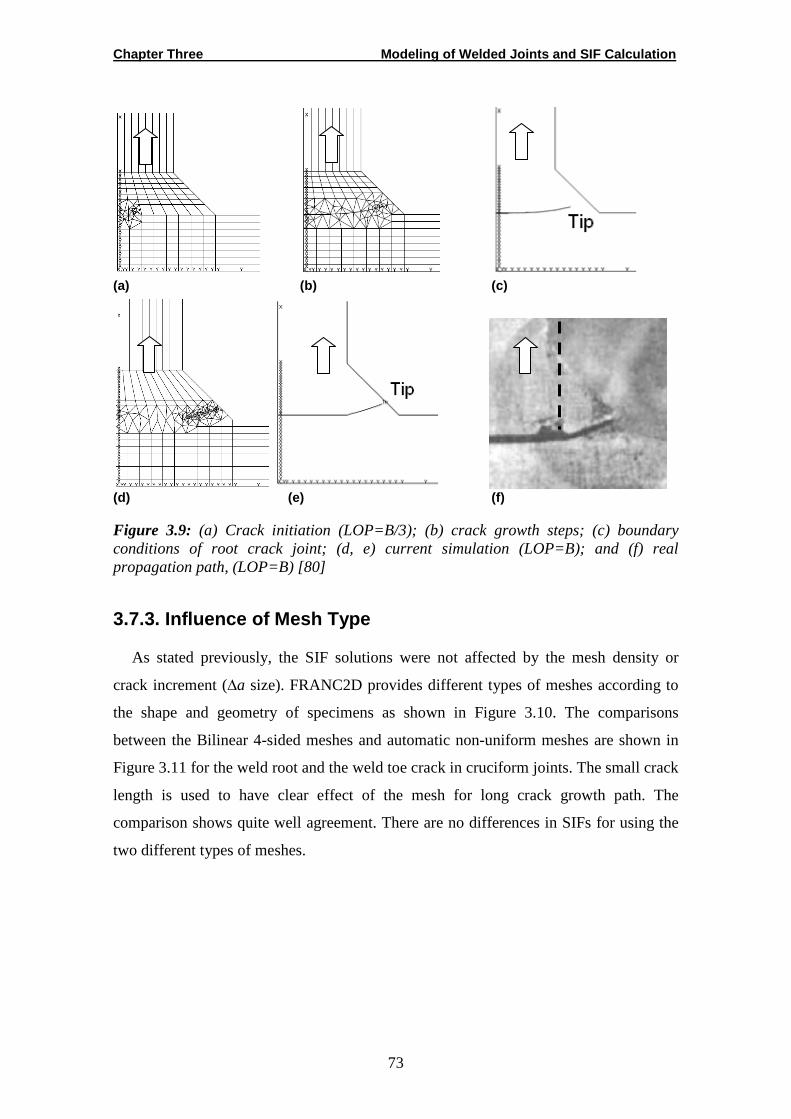
Chapter Three Modeling of Welded Joints and SIF Calculation
73
(a) (b) (c)
(d) (e) (f)
Figure 3.9: (a) Crack initiation (LOP=B/3); (b) crack growth steps; (c) boundary conditions of root crack joint; (d, e) current simulation (LOP=B); and (f) real propagation path, (LOP=B) [80]
3.7.3. Influence of Mesh Type
As stated previously, the SIF solutions were not affected by the mesh density or
crack increment (∆a size). FRANC2D provides different types of meshes according to
the shape and geometry of specimens as shown in Figure 3.10. The comparisons
between the Bilinear 4-sided meshes and automatic non-uniform meshes are shown in
Figure 3.11 for the weld root and the weld toe crack in cruciform joints. The small crack
length is used to have clear effect of the mesh for long crack growth path. The
comparison shows quite well agreement. There are no differences in SIFs for using the
two different types of meshes.
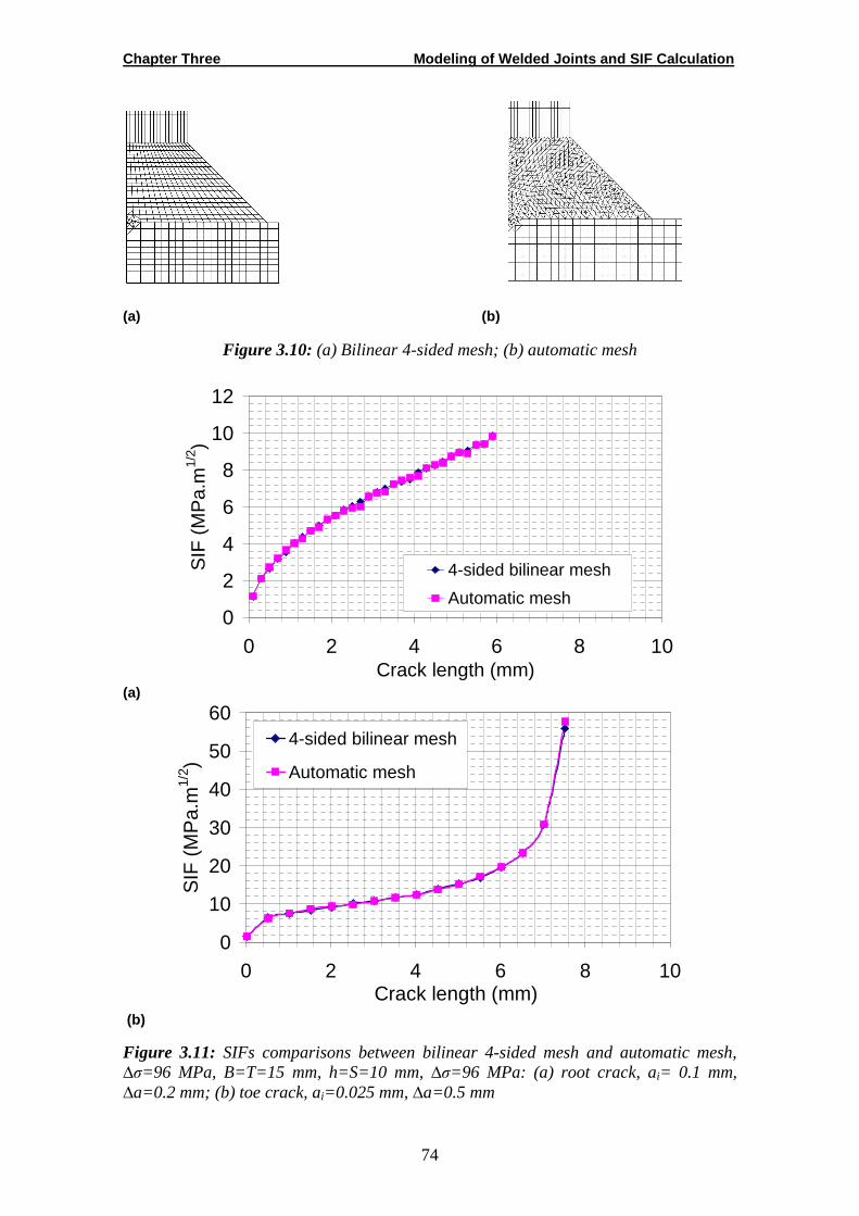
Chapter Three Modeling of Welded Joints and SIF Calculation
74
(a) (b)
Figure 3.10: (a) Bilinear 4-sided mesh; (b) automatic mesh
0
2
4
6
8
10
12
0 2 4 6 8 10Crack length (mm)
SIF
(M
Pa.
m1/
2 )
4-sided bilinear mesh
Automatic mesh
(a)
0
10
20
30
40
50
60
0 2 4 6 8 10Crack length (mm)
SIF
(M
Pa.
m1/
2 )
4-sided bilinear mesh
Automatic mesh
(b)
Figure 3.11: SIFs comparisons between bilinear 4-sided mesh and automatic mesh, ∆σ=96 MPa, B=T=15 mm, h=S=10 mm, ∆σ=96 MPa: (a) root crack, ai= 0.1 mm, ∆a=0.2 mm; (b) toe crack, ai=0.025 mm, ∆a=0.5 mm
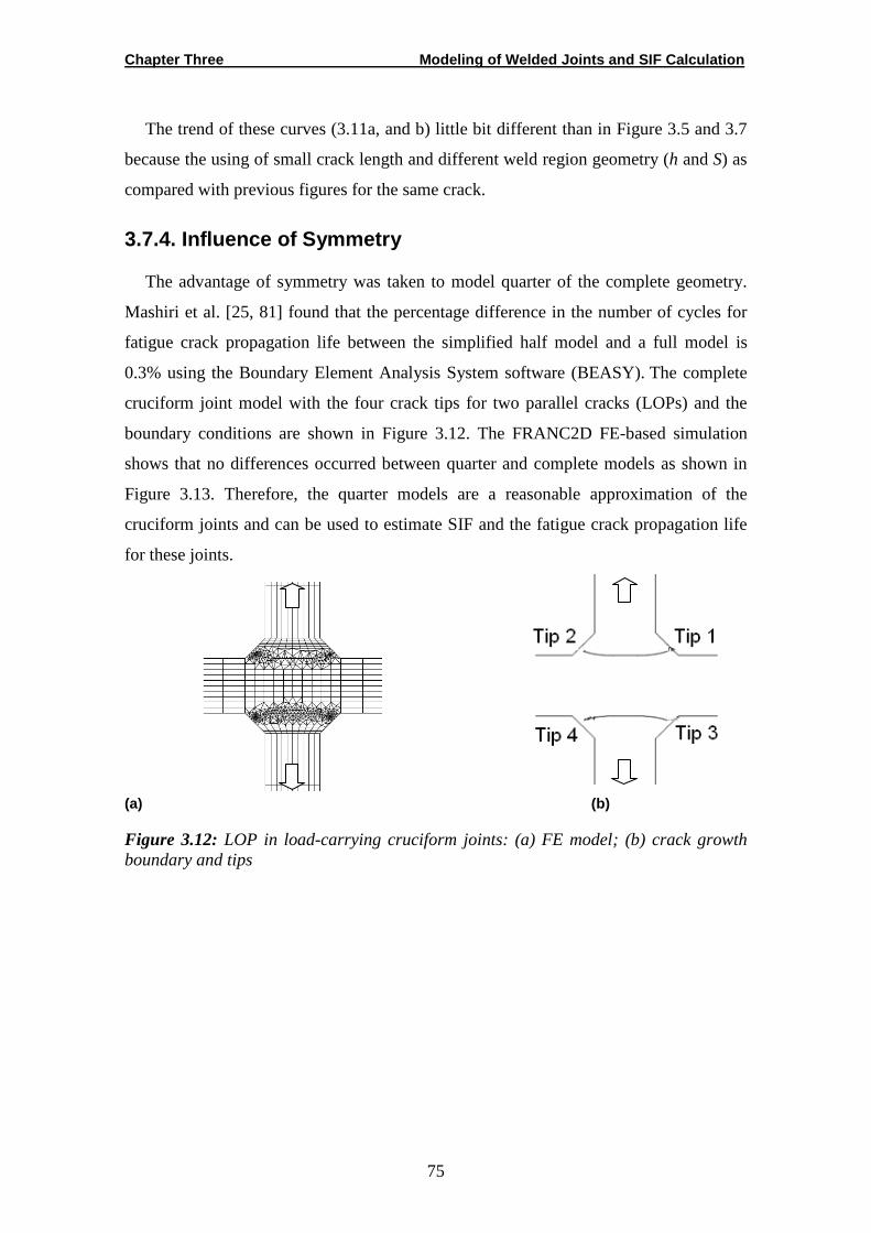
Chapter Three Modeling of Welded Joints and SIF Calculation
75
The trend of these curves (3.11a, and b) little bit different than in Figure 3.5 and 3.7
because the using of small crack length and different weld region geometry (h and S) as
compared with previous figures for the same crack.
3.7.4. Influence of Symmetry
The advantage of symmetry was taken to model quarter of the complete geometry.
Mashiri et al. [25, 81] found that the percentage difference in the number of cycles for
fatigue crack propagation life between the simplified half model and a full model is
0.3% using the Boundary Element Analysis System software (BEASY). The complete
cruciform joint model with the four crack tips for two parallel cracks (LOPs) and the
boundary conditions are shown in Figure 3.12. The FRANC2D FE-based simulation
shows that no differences occurred between quarter and complete models as shown in
Figure 3.13. Therefore, the quarter models are a reasonable approximation of the
cruciform joints and can be used to estimate SIF and the fatigue crack propagation life
for these joints.
(a) (b)
Figure 3.12: LOP in load-carrying cruciform joints: (a) FE model; (b) crack growth boundary and tips
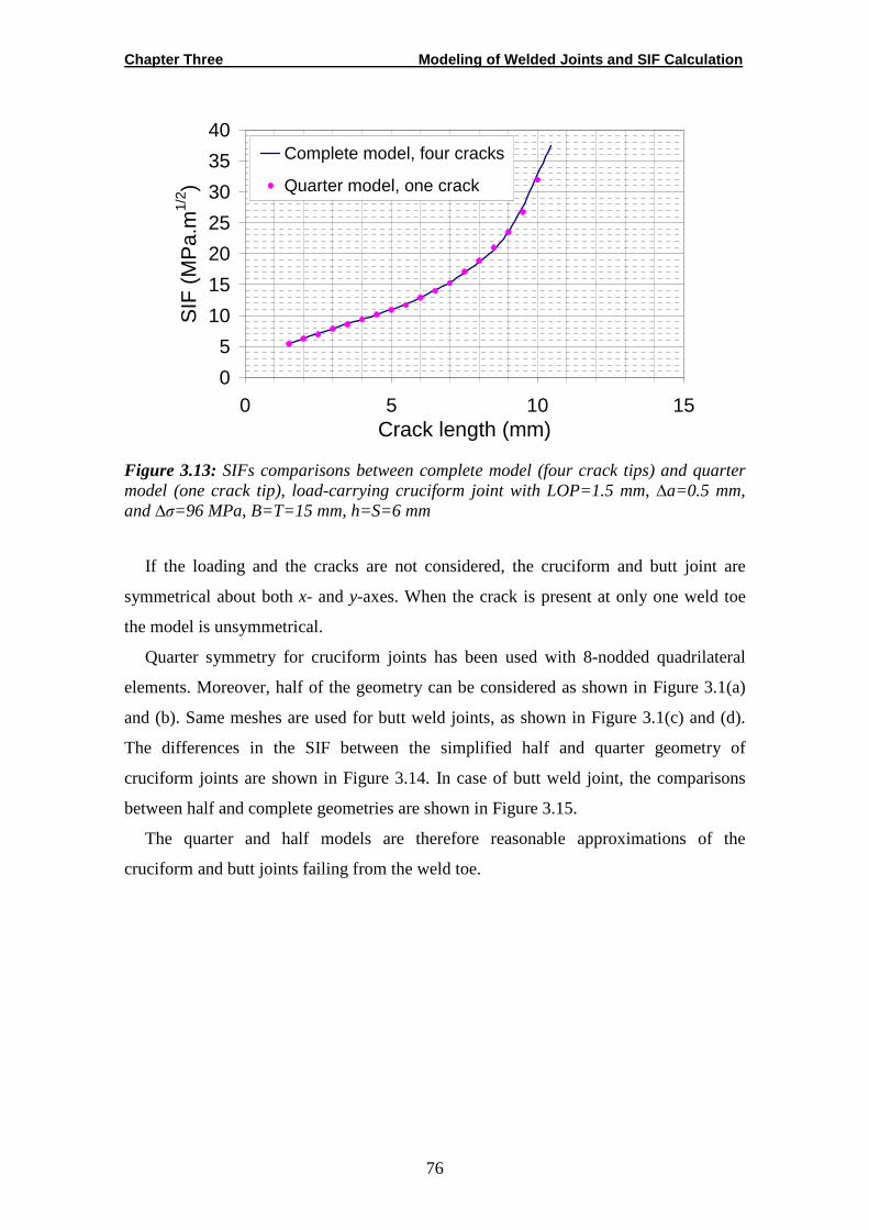
Chapter Three Modeling of Welded Joints and SIF Calculation
76
0
5
10
15
20
25
30
35
40
0 5 10 15Crack length (mm)
SIF
(M
Pa.
m1/
2 )
Complete model, four cracks
Quarter model, one crack
Figure 3.13: SIFs comparisons between complete model (four crack tips) and quarter model (one crack tip), load-carrying cruciform joint with LOP=1.5 mm, ∆a=0.5 mm, and ∆σ=96 MPa, B=T=15 mm, h=S=6 mm
If the loading and the cracks are not considered, the cruciform and butt joint are
symmetrical about both x- and y-axes. When the crack is present at only one weld toe
the model is unsymmetrical.
Quarter symmetry for cruciform joints has been used with 8-nodded quadrilateral
elements. Moreover, half of the geometry can be considered as shown in Figure 3.1(a)
and (b). Same meshes are used for butt weld joints, as shown in Figure 3.1(c) and (d).
The differences in the SIF between the simplified half and quarter geometry of
cruciform joints are shown in Figure 3.14. In case of butt weld joint, the comparisons
between half and complete geometries are shown in Figure 3.15.
The quarter and half models are therefore reasonable approximations of the
cruciform and butt joints failing from the weld toe.

Chapter Three Modeling of Welded Joints and SIF Calculation
77
0
10
20
30
40
50
60
0 2 4 6Crack length (mm)
SIF
(M
Pa.
m1/
2 )Quarter symmetry
Half symmetry
Figure 3.14: SIFs comparison between half and quarter non-load carrying cruciform joints, toe crack, ∆σ=200 MPa, ai=0.1 mm, ∆a=0.5 mm, B=T=12 mm, h=S=8.5 mm
0
20
40
60
80
100
120
140
0 2 4 6 8Crack length (mm)
SIF
(M
Pa.
m1/
2 )
Complete jointHalf symmetry
Figure 3.15: SIFs comparison between half and complete transverse butt weld joints, toe crack, ∆σ=104 MPa, ai=0.1 mm, ∆a=0.5 mm, thickness=10 mm
3.8. Selection of the Notch Cases
Typical notch cases which are used in this work are presented in Table 3.1. In
parallel joints toe cracks and LOP are frequently encountered defects.
Toe cracks have been simulated in case of non-load carrying welded joints, namely
cruciform and butt welded joints where the weld metals have been assumed as complete
penetration. The root cracks are found in load-carrying joints.
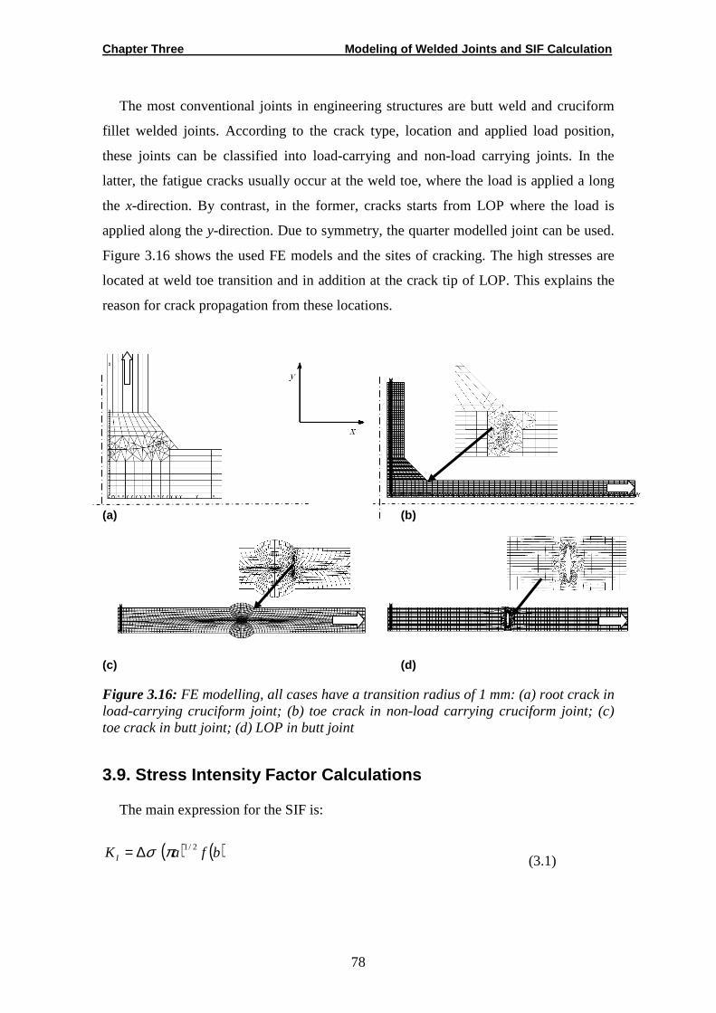
Chapter Three Modeling of Welded Joints and SIF Calculation
78
The most conventional joints in engineering structures are butt weld and cruciform
fillet welded joints. According to the crack type, location and applied load position,
these joints can be classified into load-carrying and non-load carrying joints. In the
latter, the fatigue cracks usually occur at the weld toe, where the load is applied a long
the x-direction. By contrast, in the former, cracks starts from LOP where the load is
applied along the y-direction. Due to symmetry, the quarter modelled joint can be used.
Figure 3.16 shows the used FE models and the sites of cracking. The high stresses are
located at weld toe transition and in addition at the crack tip of LOP. This explains the
reason for crack propagation from these locations.
(a) (b)
(c) (d)
Figure 3.16: FE modelling, all cases have a transition radius of 1 mm: (a) root crack in load-carrying cruciform joint; (b) toe crack in non-load carrying cruciform joint; (c) toe crack in butt joint; (d) LOP in butt joint
3.9. Stress Intensity Factor Calculations
The main expression for the SIF is:
( ) ( )bfaK I2/1πσ∆=
(3.1)
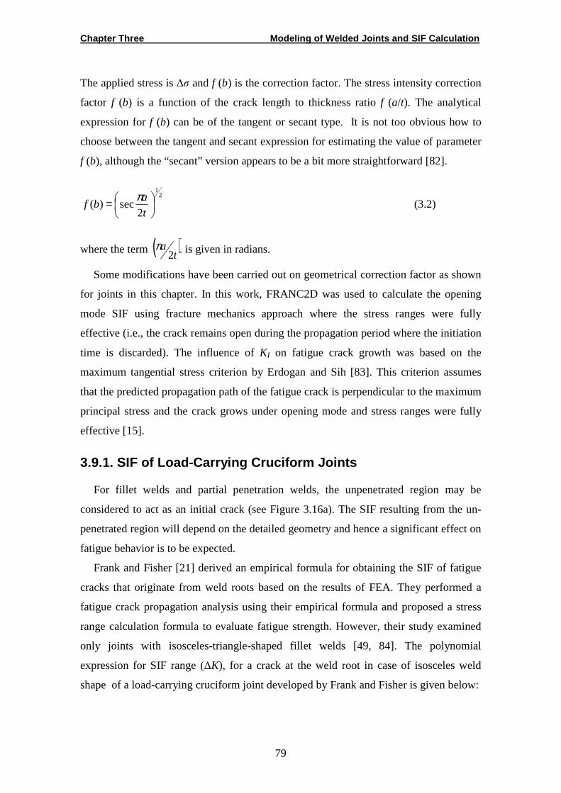
Chapter Three Modeling of Welded Joints and SIF Calculation
79
The applied stress is ∆σ and f (b) is the correction factor. The stress intensity correction
factor f (b) is a function of the crack length to thickness ratio f (a/t). The analytical
expression for f (b) can be of the tangent or secant type. It is not too obvious how to
choose between the tangent and secant expression for estimating the value of parameter
f (b), although the “secant” version appears to be a bit more straightforward [82].
21
2sec)(
=t
abf
π (3.2)
where the term ( )ta2
π is given in radians.
Some modifications have been carried out on geometrical correction factor as shown
for joints in this chapter. In this work, FRANC2D was used to calculate the opening
mode SIF using fracture mechanics approach where the stress ranges were fully
effective (i.e., the crack remains open during the propagation period where the initiation
time is discarded). The influence of KI on fatigue crack growth was based on the
maximum tangential stress criterion by Erdogan and Sih [83]. This criterion assumes
that the predicted propagation path of the fatigue crack is perpendicular to the maximum
principal stress and the crack grows under opening mode and stress ranges were fully
effective [15].
3.9.1. SIF of Load-Carrying Cruciform Joints
For fillet welds and partial penetration welds, the unpenetrated region may be
considered to act as an initial crack (see Figure 3.16a). The SIF resulting from the un-
penetrated region will depend on the detailed geometry and hence a significant effect on
fatigue behavior is to be expected.
Frank and Fisher [21] derived an empirical formula for obtaining the SIF of fatigue
cracks that originate from weld roots based on the results of FEA. They performed a
fatigue crack propagation analysis using their empirical formula and proposed a stress
range calculation formula to evaluate fatigue strength. However, their study examined
only joints with isosceles-triangle-shaped fillet welds [49, 84]. The polynomial
expression for SIF range (∆K), for a crack at the weld root in case of isosceles weld
shape of a load-carrying cruciform joint developed by Frank and Fisher is given below:
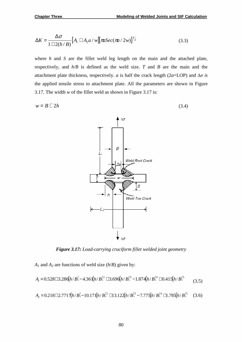
Chapter Three Modeling of Welded Joints and SIF Calculation
80
[ ][ ] 21
21 )2/(/)/(21
waaSecwaAABh
K ππσ
++
∆=∆ (3.3)
where h and S are the fillet weld leg length on the main and the attached plate,
respectively, and h/B is defined as the weld size. T and B are the main and the
attachment plate thickness, respectively. a is half the crack length (2a=LOP) and ∆σ is
the applied tensile stress to attachment plate. All the parameters are shown in Figure
3.17. The width w of the fillet weld as shown in Figure 3.17 is:
hBw 2+= (3.4)
Figure 3.17: Load-carrying cruciform fillet welded joint geometry
A1 and A2 are functions of weld size (h/B) given by:
( ) ( ) ( ) ( ) ( )54321 /415.0/874.1/696.3/361.4/286.3528.0 BhBhBhBhBhA +−+−+= (3.5)
( ) ( ) ( ) ( ) ( )54322 /785.1/775.7/122.13/171.10/7717.2218.0 BhBhBhBhBhA +−+−+= (3.6)

Chapter Three Modeling of Welded Joints and SIF Calculation
81
The International Institute of Welding (IIW) adopted Frank, Fisher formula’s for the
SIF which is valid for h/B from 0.2 to 1.2 and for (a/w) from 0.0 to 0.7 [21]. This
formula was then improved by British Standards Institution PD6493 [85] and by
BSI7910 [86], where the range of the SIF, ∆K, can be written as:
w
aaSecMK kI
ππσ∆=∆ (3.7)
The parameter KI is known as the opening mode-I stress intensity and represents the
strength of the stress surrounding the crack tip. Mk is the stress concentration
magnification factor which is defined as the ratio of the SIF of a cracked plate with a
stress concentration to the SIF with the same cracked plate without the stress
concentration [77].
2
210
22
+
+=w
aA
w
aAAM k (3.8)
The values of A0, A1 and A2 for equal leg length fillet welds and unity ratio of main
plate to attachment plate thickness are as follows [19]:
−=B
hA 343.0956.00 (3.9)
432
1 741.2704.9220.12210.6219.1
−
+
−
+−=B
h
B
h
B
h
B
hA (3.10)
432
2 513.2541.9299.13938.7954.1
+
−
+
−=B
h
B
h
B
h
B
hA (3.11)
The limits of validity for this formula are within the following range:
,1=T
B 2.12.0 ⟨⟨
B
h , and, 7.0
21.0 ⟨⟨
w
a
In all above formulas, the unity leg lengths have been assumed (h=S). Motarjemi et
al. [19] calculated numerically the SIFs for cruciform and T-steel welded joints using
ABAQUS. SIF results of the cruciform joint were firstly compared with the above
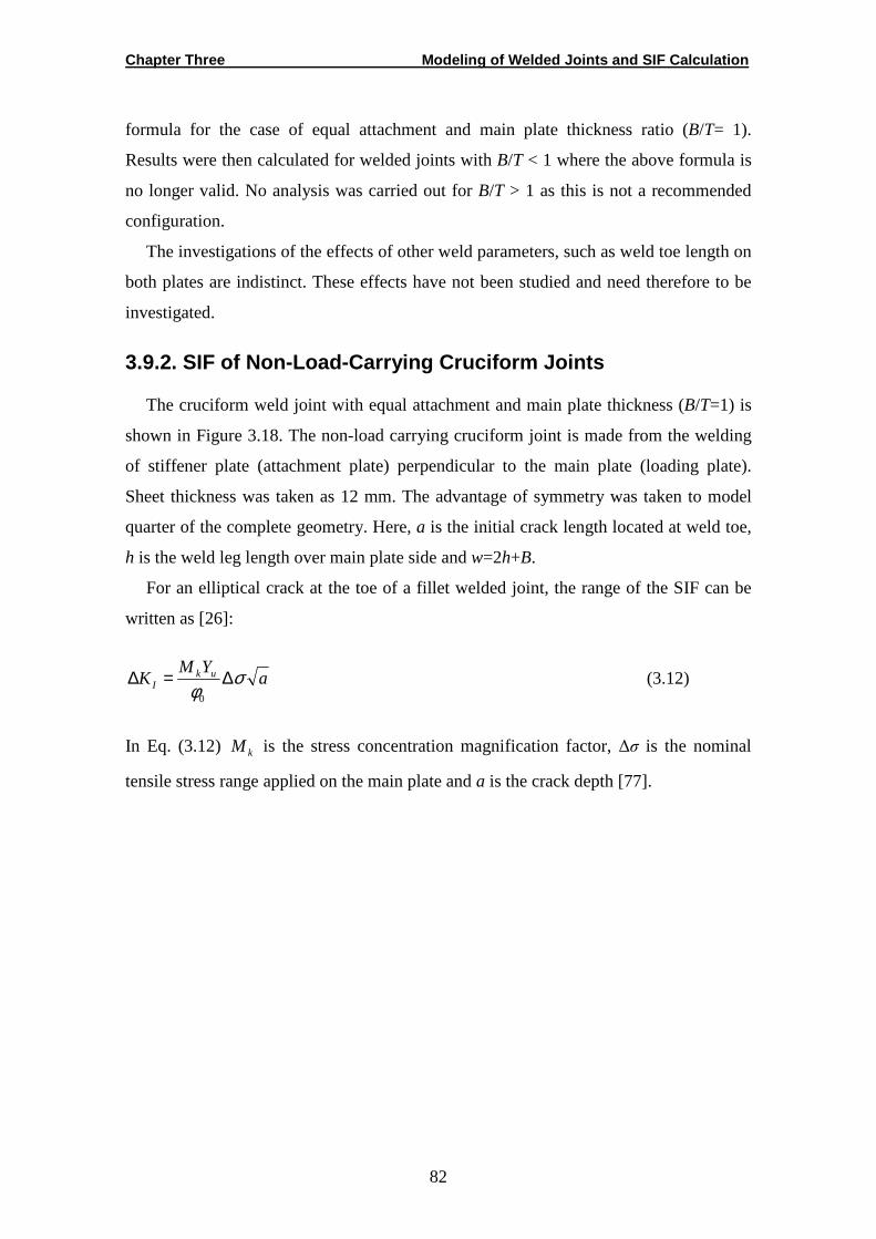
Chapter Three Modeling of Welded Joints and SIF Calculation
82
formula for the case of equal attachment and main plate thickness ratio (B/T= 1).
Results were then calculated for welded joints with B/T < 1 where the above formula is
no longer valid. No analysis was carried out for B/T > 1 as this is not a recommended
configuration.
The investigations of the effects of other weld parameters, such as weld toe length on
both plates are indistinct. These effects have not been studied and need therefore to be
investigated.
3.9.2. SIF of Non-Load-Carrying Cruciform Joints
The cruciform weld joint with equal attachment and main plate thickness (B/T=1) is
shown in Figure 3.18. The non-load carrying cruciform joint is made from the welding
of stiffener plate (attachment plate) perpendicular to the main plate (loading plate).
Sheet thickness was taken as 12 mm. The advantage of symmetry was taken to model
quarter of the complete geometry. Here, a is the initial crack length located at weld toe,
h is the weld leg length over main plate side and w=2h+B.
For an elliptical crack at the toe of a fillet welded joint, the range of the SIF can be
written as [26]:
aYM
K ukI σ
φ∆=∆
0
(3.12)
In Eq. (3.12) kM is the stress concentration magnification factor, ∆σ is the nominal
tensile stress range applied on the main plate and a is the crack depth [77].
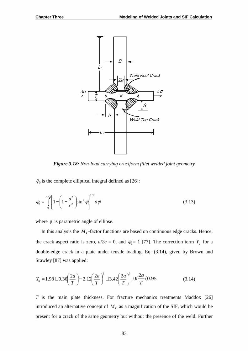
Chapter Three Modeling of Welded Joints and SIF Calculation
83
Figure 3.18: Non-load carrying cruciform fillet welded joint geometry
0φ is the complete elliptical integral defined as [26]:
φφφπ
dc
a2/12/
0
22
2
0 sin11∫
−−= (3.13)
where φ is parametric angle of ellipse.
In this analysis the kM -factor functions are based on continuous edge cracks. Hence,
the crack aspect ratio is zero, a/2c = 0, and 0φ = 1 [77]. The correction term uY for a
double-edge crack in a plate under tensile loading, Eq. (3.14), given by Brown and
Srawley [87] was applied:
322
42.32
12.22
36.098.1
+
−
+=T
a
T
a
T
aYu , 95.0
20 ⟨⟨
T
a (3.14)
T is the main plate thickness. For fracture mechanics treatments Maddox [26]
introduced an alternative concept of kM as a magnification of the SIF, which would be
present for a crack of the same geometry but without the presence of the weld. Further
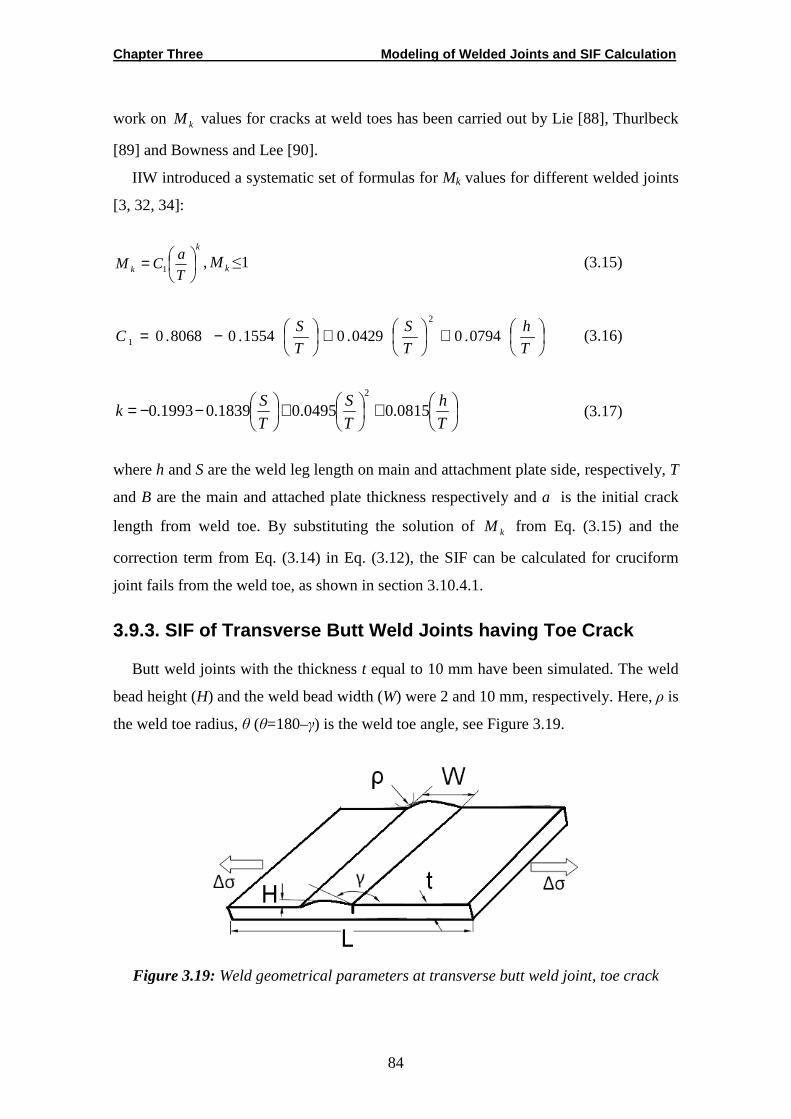
Chapter Three Modeling of Welded Joints and SIF Calculation
84
work on kM values for cracks at weld toes has been carried out by Lie [88], Thurlbeck
[89] and Bowness and Lee [90].
IIW introduced a systematic set of formulas for Mk values for different welded joints
[3, 32, 34]:
k
k T
aCM
= 1 , kM ≤1 (3.15)
+
+
−=T
h
T
S
T
SC 0794.00429.01554.08068.0
2
1 (3.16)
+
+
−−=T
h
T
S
T
Sk 0815.00495.01839.01993.0
2
(3.17)
where h and S are the weld leg length on main and attachment plate side, respectively, T
and B are the main and attached plate thickness respectively and a is the initial crack
length from weld toe. By substituting the solution of kM from Eq. (3.15) and the
correction term from Eq. (3.14) in Eq. (3.12), the SIF can be calculated for cruciform
joint fails from the weld toe, as shown in section 3.10.4.1.
3.9.3. SIF of Transverse Butt Weld Joints having To e Crack
Butt weld joints with the thickness t equal to 10 mm have been simulated. The weld
bead height (H) and the weld bead width (W) were 2 and 10 mm, respectively. Here, ρ is
the weld toe radius, θ (θ=180–γ) is the weld toe angle, see Figure 3.19.
Figure 3.19: Weld geometrical parameters at transverse butt weld joint, toe crack
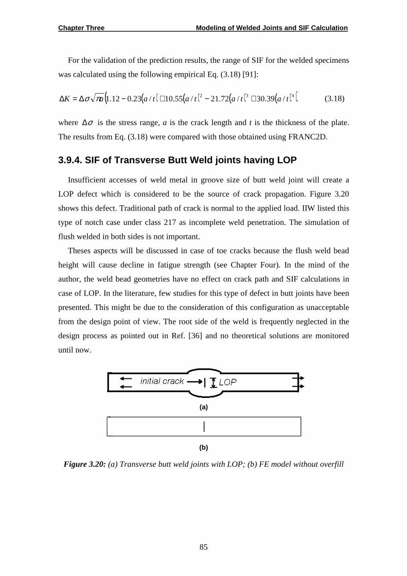
Chapter Three Modeling of Welded Joints and SIF Calculation
85
For the validation of the prediction results, the range of SIF for the welded specimens
was calculated using the following empirical Eq. (3.18) [91]:
( ) ( ) ( ) ( )( )432 /39.30/72.21/55.10/23.012.1 tatatataaK +−+−∆=∆ πσ (3.18)
where σ∆ is the stress range, a is the crack length and t is the thickness of the plate.
The results from Eq. (3.18) were compared with those obtained using FRANC2D.
3.9.4. SIF of Transverse Butt Weld joints having LO P
Insufficient accesses of weld metal in groove size of butt weld joint will create a
LOP defect which is considered to be the source of crack propagation. Figure 3.20
shows this defect. Traditional path of crack is normal to the applied load. IIW listed this
type of notch case under class 217 as incomplete weld penetration. The simulation of
flush welded in both sides is not important.
Theses aspects will be discussed in case of toe cracks because the flush weld bead
height will cause decline in fatigue strength (see Chapter Four). In the mind of the
author, the weld bead geometries have no effect on crack path and SIF calculations in
case of LOP. In the literature, few studies for this type of defect in butt joints have been
presented. This might be due to the consideration of this configuration as unacceptable
from the design point of view. The root side of the weld is frequently neglected in the
design process as pointed out in Ref. [36] and no theoretical solutions are monitored
until now.
(a)
(b)
Figure 3.20: (a) Transverse butt weld joints with LOP; (b) FE model without overfill

Chapter Three Modeling of Welded Joints and SIF Calculation
86
3.10. Results and Discussion
The crack growth simulation and SIF calculation are presented in the following
sections for cruciform and butt welded joints.
3.10.1. Cruciform Fillet Weld Model
Particularly, there are competing sites for initiation of fracture at the weld toe and at
the weld root for fillet weld joints. At these points, a high stress concentration occurs
which makes these regions the easier points from which fatigue cracks may initiate [19].
It is important to recognize that for both fracture and fatigue, the cracks may initiate and
grow in the vicinity of the welds during service life even if the applied stresses are well
below the yield limit.
3.10.2. Stress Distribution
Figure 3.21 shows the stress near the weld toe is equal to 364 MPa whereas the
applied load is 200 MPa.
The maximum and minimum principal stress distributions for uniform load
distributions of cruciform without crack are shown in Figure 3.21 for uncracked edge.
The local stress will increase with existence of a crack because of the local stress field at
the crack tip of 0.1 mm will be more severe. Figure 3.22 gives the principal stress
distributions in case of presence of an edge crack.
A maximum tangential stress criterion was used to predict the crack growth direction
under mixed mode KI -KII conditions, so that according to this criterion, the crack path
direction will change automatically and was not pre-selected. In the FRANC2D, the site
and curved crack growth path of continuous toe cracks were taken into account as
shown in Figures 3.23 and 3.24, respectively. Normally this kind of non-load carrying
welded attachments always fails from the weld toe as shown in Figure 3.25.
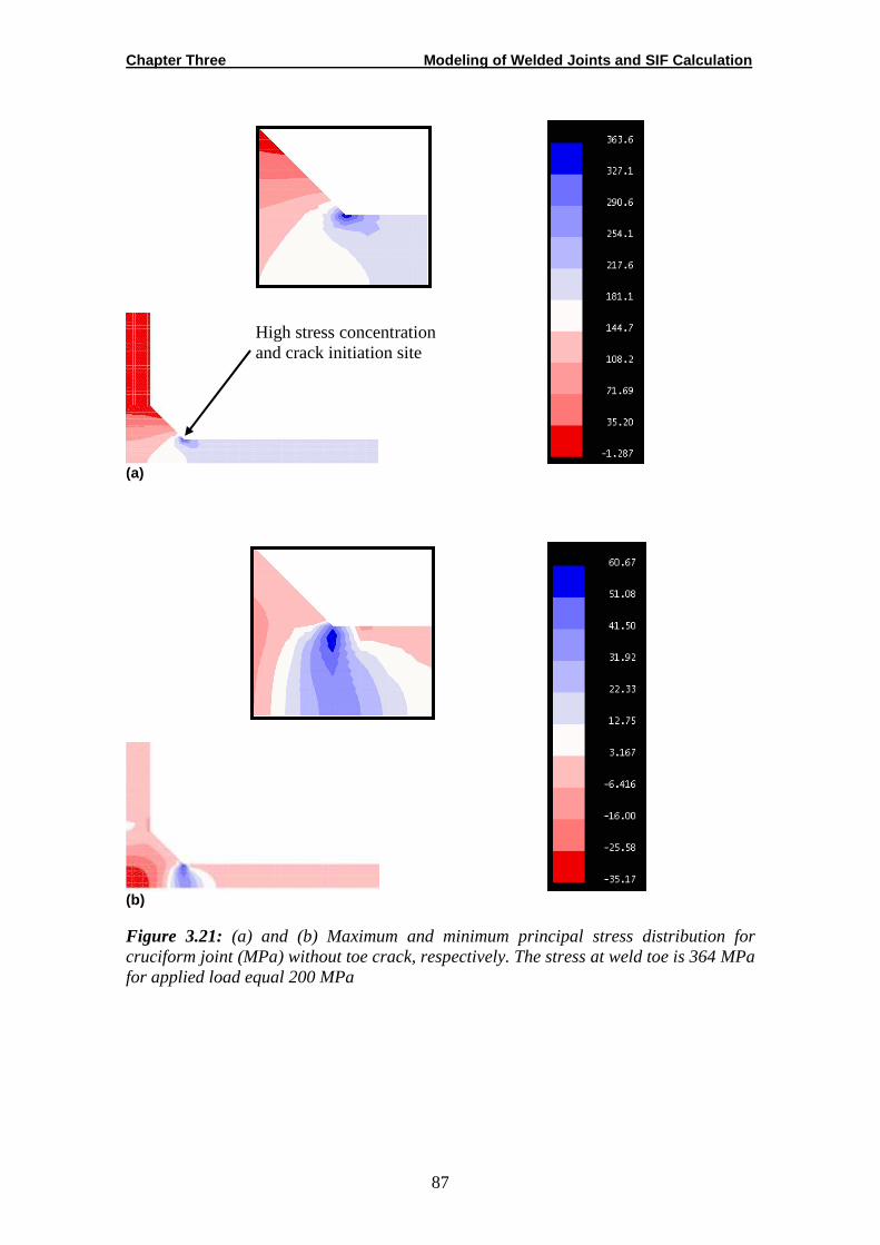
Chapter Three Modeling of Welded Joints and SIF Calculation
87
(a)
(b)
Figure 3.21: (a) and (b) Maximum and minimum principal stress distribution for cruciform joint (MPa) without toe crack, respectively. The stress at weld toe is 364 MPa for applied load equal 200 MPa
High stress concentration and crack initiation site
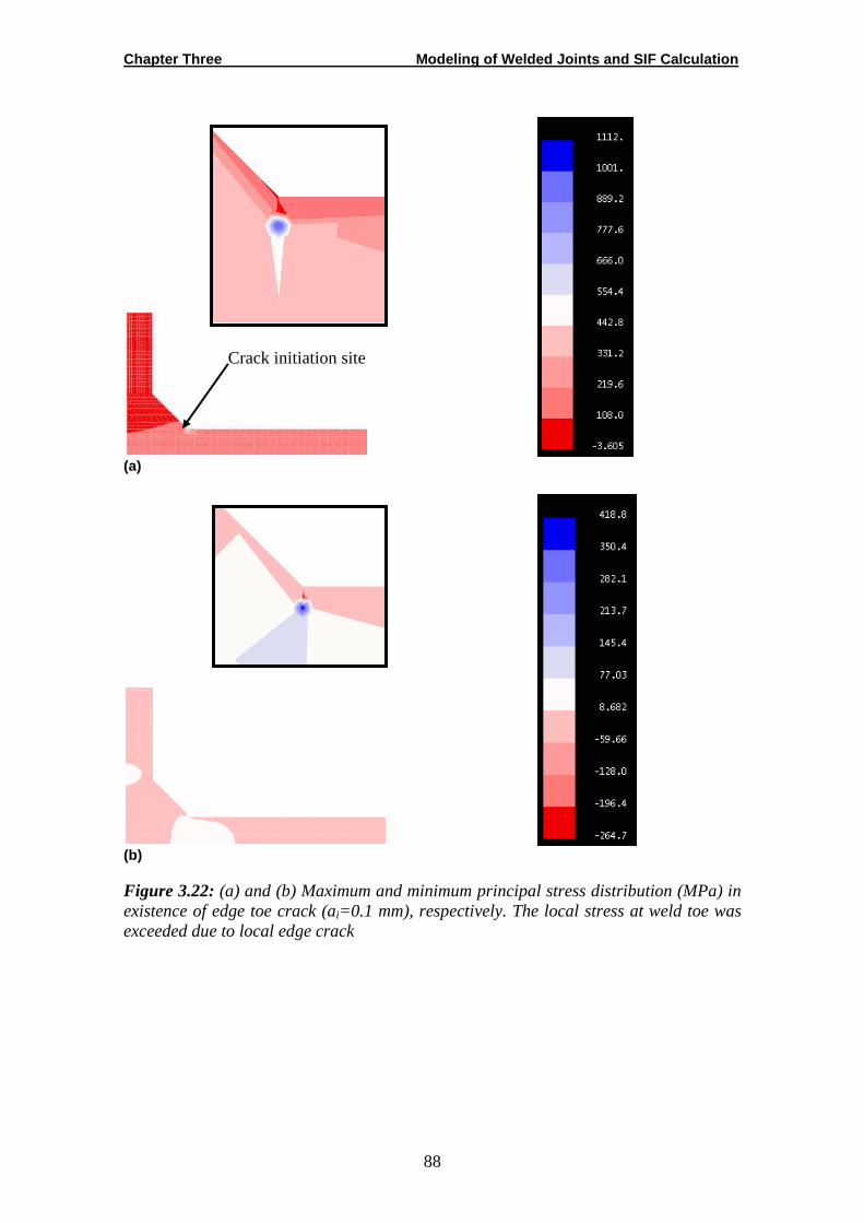
Chapter Three Modeling of Welded Joints and SIF Calculation
88
(a)
(b)
Figure 3.22: (a) and (b) Maximum and minimum principal stress distribution (MPa) in existence of edge toe crack (ai=0.1 mm), respectively. The local stress at weld toe was exceeded due to local edge crack
Crack initiation site
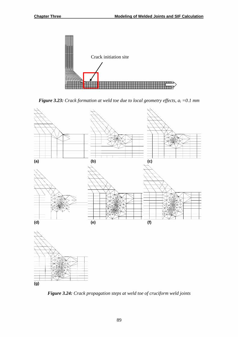
Chapter Three Modeling of Welded Joints and SIF Calculation
89
Figure 3.23: Crack formation at weld toe due to local geometry effects, ai =0.1 mm
(a) (b) (c)
(d) (e) (f)
(g)
Figure 3.24: Crack propagation steps at weld toe of cruciform weld joints
Crack initiation site

Chapter Three Modeling of Welded Joints and SIF Calculation
90
Figure 3.25: Crack deformation of cruciform weld joint
3.10.3. Butt Weld Model
The same steel was used for welding the butt welded joints. Weld toe crack initiated
and grows through the sheet thickness of 10 mm.
Figure 3.1(c, and d) shows the modelling and boundary conditions of butt weld joint
that are used to calculate the SIF. Figures 3.26 and 3.27 show the crack initiation and
propagation, respectively. The final crack deformation is shown in Figure 3.28.
Figure 3.26: Screenshot from FRANC2D crack tip at weld toe, ai =0.1 mm
Figure 3.27: Screenshot from FRANC2D of the crack growth direction, toe crack
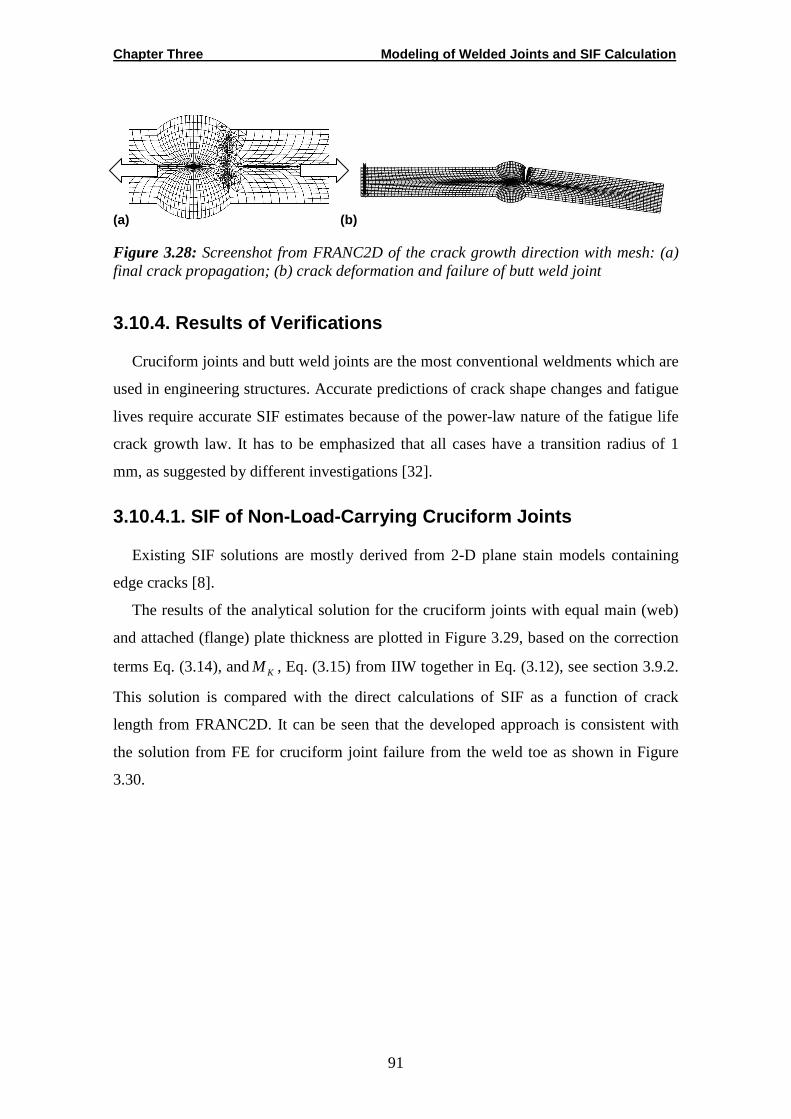
Chapter Three Modeling of Welded Joints and SIF Calculation
91
(a) (b)
Figure 3.28: Screenshot from FRANC2D of the crack growth direction with mesh: (a) final crack propagation; (b) crack deformation and failure of butt weld joint
3.10.4. Results of Verifications
Cruciform joints and butt weld joints are the most conventional weldments which are
used in engineering structures. Accurate predictions of crack shape changes and fatigue
lives require accurate SIF estimates because of the power-law nature of the fatigue life
crack growth law. It has to be emphasized that all cases have a transition radius of 1
mm, as suggested by different investigations [32].
3.10.4.1. SIF of Non-Load-Carrying Cruciform Joints
Existing SIF solutions are mostly derived from 2-D plane stain models containing
edge cracks [8].
The results of the analytical solution for the cruciform joints with equal main (web)
and attached (flange) plate thickness are plotted in Figure 3.29, based on the correction
terms Eq. (3.14), and KM , Eq. (3.15) from IIW together in Eq. (3.12), see section 3.9.2.
This solution is compared with the direct calculations of SIF as a function of crack
length from FRANC2D. It can be seen that the developed approach is consistent with
the solution from FE for cruciform joint failure from the weld toe as shown in Figure
3.30.
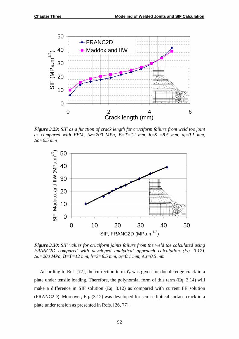
Chapter Three Modeling of Welded Joints and SIF Calculation
92
0
10
20
30
40
50
0 2 4 6Crack length (mm)
SIF
(M
Pa.
m1/
2 )
FRANC2DMaddox and IIW
Figure 3.29: SIF as a function of crack length for cruciform failure from weld toe joint as compared with FEM, ∆σ=200 MPa, B=T=12 mm, h=S =8.5 mm, ai=0.1 mm, ∆a=0.5 mm
0
10
20
30
40
50
0 10 20 30 40 50SIF, FRANC2D (MPa.m1/2)
SIF
, Mad
dox
and
IIW (
MP
a.m
1/2 )
Figure 3.30: SIF values for cruciform joints failure from the weld toe calculated using FRANC2D compared with developed analytical approach calculation (Eq. 3.12). ∆σ=200 MPa, B=T=12 mm, h=S=8.5 mm, ai=0.1 mm, ∆a=0.5 mm
According to Ref. [77], the correction term Yu was given for double edge crack in a
plate under tensile loading. Therefore, the polynomial form of this term (Eq. 3.14) will
make a difference in SIF solution (Eq. 3.12) as compared with current FE solution
(FRANC2D). Moreover, Eq. (3.12) was developed for semi-elliptical surface crack in a
plate under tension as presented in Refs. [26, 77].
Chapter Three Modeling of Welded Joints and SIF Calculation
93
FRANC2D has predicted the solution for edge crack at the weld toe of cruciform
fillet weld joint. This single edge crack has a different crack path according to the
assumption of maximum stress criteria. The crack has inclined at first with respect to
the applied load and then turned to direction normal to the applied load (see Figure
3.24). Therefore, the differences started at the beginning of crack propagation and after
some millimeters, there are some consistencies with analytical solution and the two
solutions become closer for larger crack depths (see Figure 3.29). The reason is that the
crack path will become similar to the behavior of double edge crack in a plate under
tensile loading.
3.10.4.2. SIF of Load-Carrying Cruciform Joints
From literature [16, 17, 18] it is evident that most of the investigations on fatigue life
prediction of fillet welded joints are based on the weld toe failure. Some other studies
have considered the fatigue behavior of fillet welded cruciform joints failing from the
root region.
In studies [19, 20, 21, 22, 54, 84, 92] the fatigue behavior and SIF of cruciform and
T-welded joints of steels failing from the root (LOP) have been studied.
The maximum stress intensities develop when the plane of the crack path is normal
to the direction of the primary tensile stress. The SIFs for cruciform joints with LOP
were calculated using FRANC2D and were compared with solutions from Frank and
Fisher [21], BSI 7910 [14, 85] and IIW [3, 34] and are compared in Figure 3.31.
To study the effect of curved crack path and convergence of results, two FE solutions
have been used. In the first solution, the SIFs are calculated only for initial crack step,
i.e., ai= 1.5, 2, 5, 7.5, 9, 10, and 11.5 mm, where the crack growth plane still straight
forward. In the second solution, the SIF was calculated, when the initial LOP crack is
allowed to grow to its final length (from 2ai=LOP to failure) i.e., the crack growth plane
is curved. The comparison of both solutions in Figure 3.31 shows that the solutions
from BSI 7910 are more realistic and have quite good agreement with FEA, more than
IIW solution. The latter solution is worse because the non-modified SIFs equation was
used.
The first FRANC2D calculation is more consistent with that from BSI up to the
finally calculated crack length, however, the first FRANC solution assumed a straight
line crack path normal to the applied load.
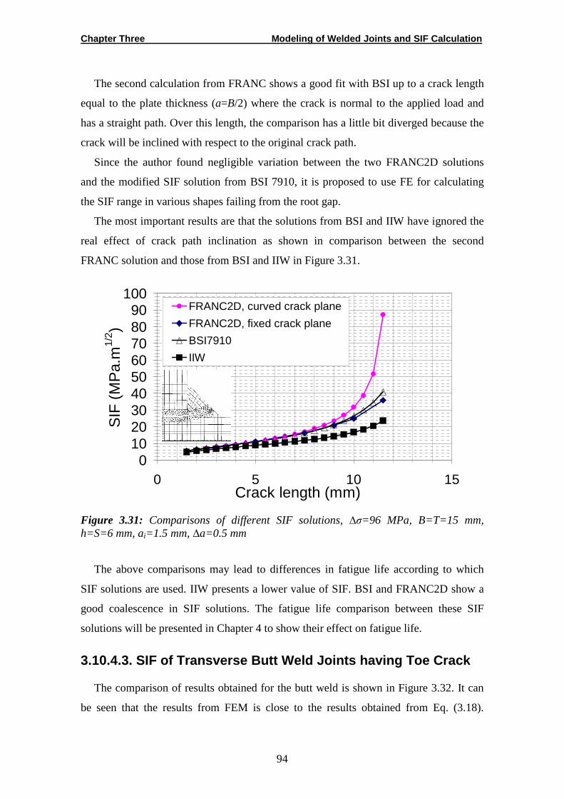
Chapter Three Modeling of Welded Joints and SIF Calculation
94
The second calculation from FRANC shows a good fit with BSI up to a crack length
equal to the plate thickness (a=B/2) where the crack is normal to the applied load and
has a straight path. Over this length, the comparison has a little bit diverged because the
crack will be inclined with respect to the original crack path.
Since the author found negligible variation between the two FRANC2D solutions
and the modified SIF solution from BSI 7910, it is proposed to use FE for calculating
the SIF range in various shapes failing from the root gap.
The most important results are that the solutions from BSI and IIW have ignored the
real effect of crack path inclination as shown in comparison between the second
FRANC solution and those from BSI and IIW in Figure 3.31.
0102030405060708090
100
0 5 10 15Crack length (mm)
SIF
(M
Pa.
m1/
2 )
FRANC2D, curved crack plane
FRANC2D, fixed crack plane
BSI7910
IIW
Figure 3.31: Comparisons of different SIF solutions, ∆σ=96 MPa, B=T=15 mm, h=S=6 mm, ai=1.5 mm, ∆a=0.5 mm
The above comparisons may lead to differences in fatigue life according to which
SIF solutions are used. IIW presents a lower value of SIF. BSI and FRANC2D show a
good coalescence in SIF solutions. The fatigue life comparison between these SIF
solutions will be presented in Chapter 4 to show their effect on fatigue life.
3.10.4.3. SIF of Transverse Butt Weld Joints having Toe Crack
The comparison of results obtained for the butt weld is shown in Figure 3.32. It can
be seen that the results from FEM is close to the results obtained from Eq. (3.18).

Chapter Three Modeling of Welded Joints and SIF Calculation
95
FRANC2D compares well with empirical equations and appears to be more realistic
because different deviations from ideal geometries can be realised.
0
20
40
60
80
100
120
140
0 2 4 6 8 10Crack length (mm)
SIF
(M
Pa.
m1/
2 )FRANC2D
Empirical solution (Eq. 3.18)
Figure 3.32: FRANC2D and empirical solutions of SIF for butt weld joint according to Broek [91], ∆σ=104 MPa, ai=0.1 mm, ∆a=0.5 mm, thickness=10 mm
3.10.4.4. SIF of Transverse Butt Weld Joints having LOP
The crack is simply propagating in direction normal to the applied load due to the
nature of these defects and this butt joint. The SIF traditionally increases as the crack
length increases as shown in Figure 3.33. There are no effects of weld bead dimensions
on the SIF results for this type of joints, i.e., the effect of weld bead height and width.
0
5
10
15
20
25
0 1 2 3 4 5Crack length (mm)
SIF
(M
Pa.
m1/
2 )
FRANC2D
Figure 3.33: SIF of transverse butt weld joint having LOP, ∆σ=104 MPa, ai=LOP=1.1 mm, ∆a=0.5 mm, thickness=10 mm
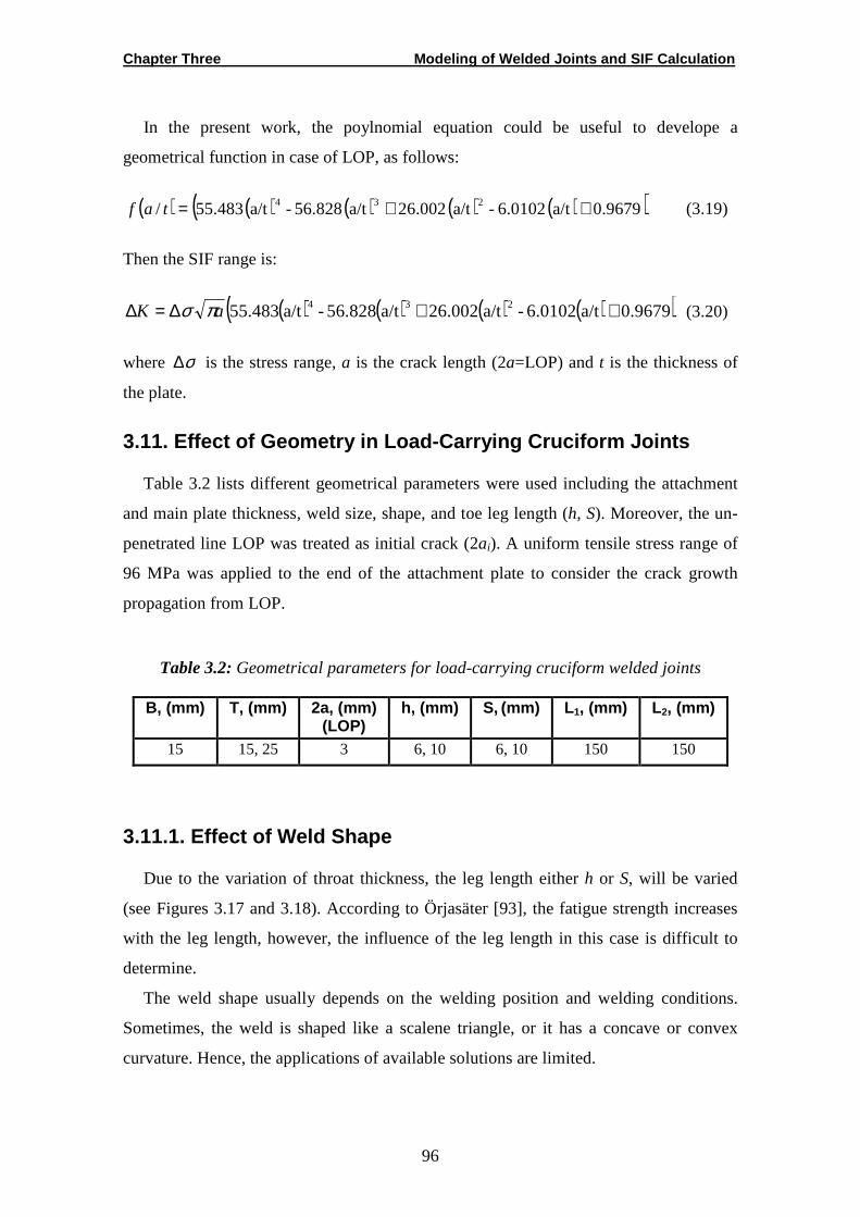
Chapter Three Modeling of Welded Joints and SIF Calculation
96
In the present work, the poylnomial equation could be useful to develope a
geometrical function in case of LOP, as follows:
( ) ( ) ( ) ( ) ( )( )0.9679 a/t6.0102 - a/t26.002 a/t56.828 - a/t55.483/ 234 ++=taf (3.19)
Then the SIF range is:
( ) ( ) ( ) ( )( )0.9679 a/t6.0102 - a/t26.002 a/t56.828 - a/t55.483 234 ++∆=∆ aK πσ (3.20)
where σ∆ is the stress range, a is the crack length (2a=LOP) and t is the thickness of
the plate.
3.11. Effect of Geometry in Load-Carrying Cruciform Joints
Table 3.2 lists different geometrical parameters were used including the attachment
and main plate thickness, weld size, shape, and toe leg length (h, S). Moreover, the un-
penetrated line LOP was treated as initial crack (2ai). A uniform tensile stress range of
96 MPa was applied to the end of the attachment plate to consider the crack growth
propagation from LOP.
Table 3.2: Geometrical parameters for load-carrying cruciform welded joints
B, (mm) T, (mm) 2a, (mm) (LOP)
h, (mm) S, (mm) L1, (mm) L2, (mm)
15 15, 25 3 6, 10 6, 10 150 150
3.11.1. Effect of Weld Shape
Due to the variation of throat thickness, the leg length either h or S, will be varied
(see Figures 3.17 and 3.18). According to Örjasäter [93], the fatigue strength increases
with the leg length, however, the influence of the leg length in this case is difficult to
determine.
The weld shape usually depends on the welding position and welding conditions.
Sometimes, the weld is shaped like a scalene triangle, or it has a concave or convex
curvature. Hence, the applications of available solutions are limited.
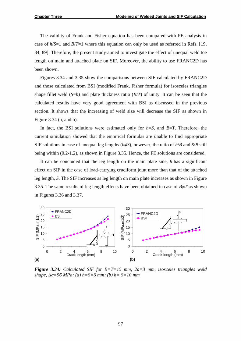
Chapter Three Modeling of Welded Joints and SIF Calculation
97
The validity of Frank and Fisher equation has been compared with FE analysis in
case of h/S=1 and B/T=1 where this equation can only be used as referred in Refs. [19,
84, 89]. Therefore, the present study aimed to investigate the effect of unequal weld toe
length on main and attached plate on SIF. Moreover, the ability to use FRANC2D has
been shown.
Figures 3.34 and 3.35 show the comparisons between SIF calculated by FRANC2D
and those calculated from BSI (modified Frank, Fisher formula) for isosceles triangles
shape fillet weld (S=h) and plate thickness ratio (B/T) of unity. It can be seen that the
calculated results have very good agreement with BSI as discussed in the previous
section. It shows that the increasing of weld size will decrease the SIF as shown in
Figure 3.34 (a, and b).
In fact, the BSI solutions were estimated only for h=S, and B=T. Therefore, the
current simulation showed that the empirical formulas are unable to find appropriate
SIF solutions in case of unequal leg lengths (h≠S), however, the ratio of h/B and S/B still
being within (0.2-1.2), as shown in Figure 3.35. Hence, the FE solutions are considered.
It can be concluded that the leg length on the main plate side, h has a significant
effect on SIF in the case of load-carrying cruciform joint more than that of the attached
leg length, S. The SIF increases as leg length on main plate increases as shown in Figure
3.35. The same results of leg length effects have been obtained in case of B≠T as shown
in Figures 3.36 and 3.37.
0
5
10
15
20
25
30
0 2 4 6 8 10Crack length (mm)
SIF
(M
Pa.
m1/
2)
FRANC2DBSI
0
5
10
15
20
25
30
0 2 4 6 8 10Crack length (mm)
SIF
(M
Pa.
m1/
2)
FRANC2DBSI
(a) (b)
Figure 3.34: Calculated SIF for B=T=15 mm, 2a=3 mm, isosceles triangles weld shape, ∆σ=96 MPa: (a) h=S=6 mm; (b) h= S=10 mm
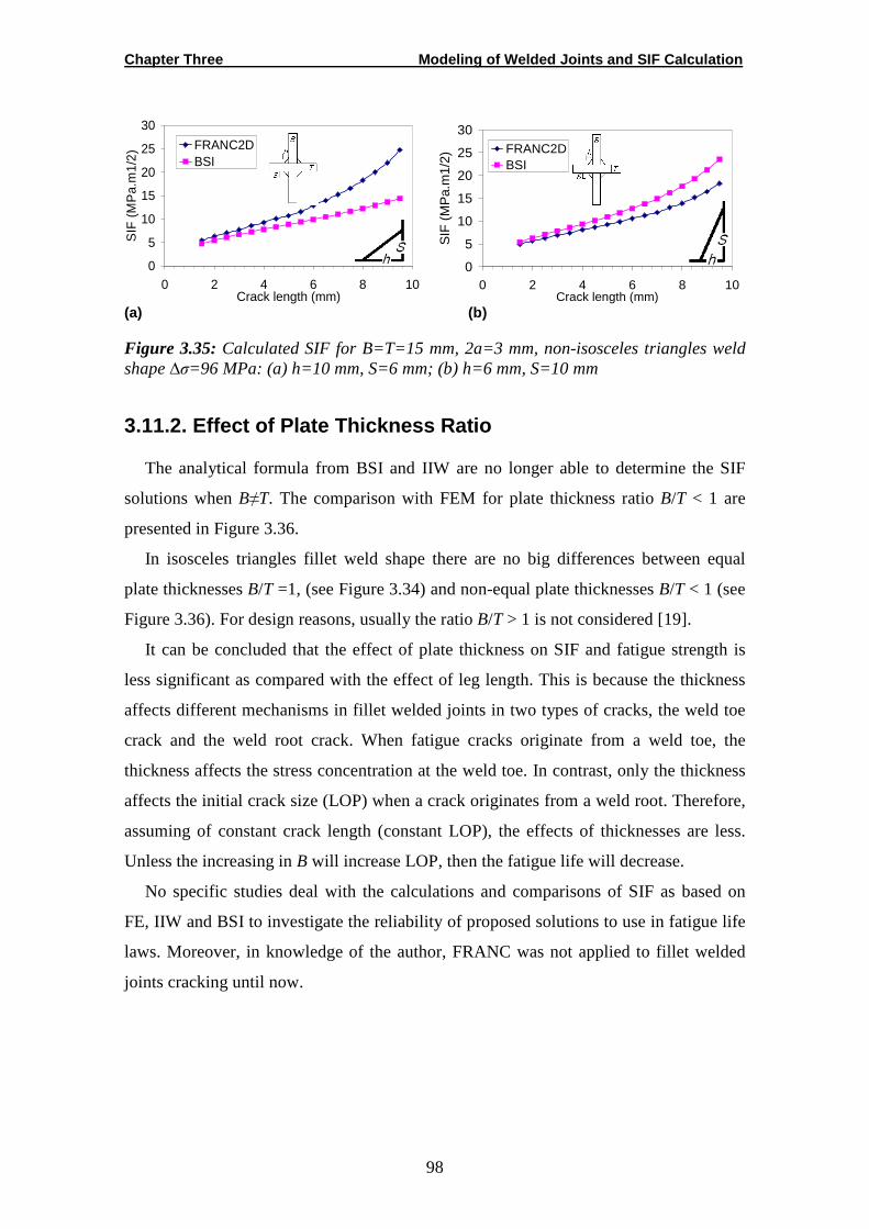
Chapter Three Modeling of Welded Joints and SIF Calculation
98
0
5
10
15
20
25
30
0 2 4 6 8 10Crack length (mm)
SIF
(M
Pa.
m1/
2)FRANC2DBSI
0
5
10
15
20
25
30
0 2 4 6 8 10Crack length (mm)
SIF
(M
Pa.
m1/
2)
FRANC2DBSI
(a) (b)
Figure 3.35: Calculated SIF for B=T=15 mm, 2a=3 mm, non-isosceles triangles weld shape ∆σ=96 MPa: (a) h=10 mm, S=6 mm; (b) h=6 mm, S=10 mm
3.11.2. Effect of Plate Thickness Ratio
The analytical formula from BSI and IIW are no longer able to determine the SIF
solutions when B≠T. The comparison with FEM for plate thickness ratio B/T < 1 are
presented in Figure 3.36.
In isosceles triangles fillet weld shape there are no big differences between equal
plate thicknesses B/T =1, (see Figure 3.34) and non-equal plate thicknesses B/T < 1 (see
Figure 3.36). For design reasons, usually the ratio B/T > 1 is not considered [19].
It can be concluded that the effect of plate thickness on SIF and fatigue strength is
less significant as compared with the effect of leg length. This is because the thickness
affects different mechanisms in fillet welded joints in two types of cracks, the weld toe
crack and the weld root crack. When fatigue cracks originate from a weld toe, the
thickness affects the stress concentration at the weld toe. In contrast, only the thickness
affects the initial crack size (LOP) when a crack originates from a weld root. Therefore,
assuming of constant crack length (constant LOP), the effects of thicknesses are less.
Unless the increasing in B will increase LOP, then the fatigue life will decrease.
No specific studies deal with the calculations and comparisons of SIF as based on
FE, IIW and BSI to investigate the reliability of proposed solutions to use in fatigue life
laws. Moreover, in knowledge of the author, FRANC was not applied to fillet welded
joints cracking until now.

Chapter Three Modeling of Welded Joints and SIF Calculation
99
0
5
10
15
20
25
30
0 2 4 6 8 10Crack length (mm)
SIF
(M
Pa.
m1/
2)FRANC2DBSI
0
5
10
15
20
25
30
0 2 4 6 8 10Crack length (mm)
SIF
(M
Pa.
m1/
2)
FRANC2DBSI
(a) (b)
Figure 3.36: Calculated SIF B=15, T=25 mm, 2a=3 mm, isosceles triangles weld shape ∆σ=96 MPa: (a) h=S=6 mm; (b) h=S=10 mm
0
5
10
15
20
25
30
0 2 4 6 8 10Crack length (mm)
SIF
(M
Pa.
m1/
2)
FRANC2D
BSI
0
5
10
15
20
25
30
0 2 4 6 8 10Crack length (mm)
SIF
(M
Pa.
m1/
2)
FRANC2D
BSI
(a) (b)
Figure 3.37: Calculated SIF B=15, T=25 mm, 2a=3 mm, non-isosceles triangles weld shape ∆σ=96 MPa: (a) h=10 mm, S=6 mm; b) h=6 mm, S=10 mm
3.12. Conclusions
The main objective of this chapter is to show the reliability of FRANC2D program to
calculate SIF in fillet welded joints. This factor will be used to calculate fatigue life.
Several formulas were used to calculate SIF via crack length.
SIF at the weld toe and weld root of cruciform and butt welded joints have been
evaluated using the FEM where the influence of the weld geometry was incorporated in
the solutions. Meanwhile, the analytical SIF solutions have been derived for transverse
butt joints having LOP.
The assumption was used that in the as-welded condition the crack remains open
during the loading cycle due to the tensile residual stresses caused by welding are high
enough. Therefore, the SIFs range corresponding to the nominal stress range is effective
and independent of the R-ratio of nominal stresses. To include the effect of crack
closure, other SIFs due to residual stresses should be calculated as will be discussed in
Chapter Three Modeling of Welded Joints and SIF Calculation
100
Chapter Five. The FRANC2D software and quadrilateral elements were used to
calculate the SIF of the joints from elementary of fracture mechanics.
This program has the ability to analyse a cracked body and to describe the singularity
ahead of the crack tip. Thus, it can be concluded that for specific crack propagation, the
SIF can be calculated under mode-I loading conditions. The efficiency of the current
calculations was demonstrated for two examples of joints. In the present study, a
developed analytical approach for toe crack in cruciform joints has been used. Frank
and Fisher’s formula was used in limited geometries in case LOP.
For the LOP forms of root cracks recommendations were given to use the modified
solution from BSI 7910 instead of that from IIW. The reason for the difference between
these two solutions (BSI and IIW) is that IIW uses the old Frank, Fisher formula
whereas recently BSI modified this formula. These difference effects will be presented
in Chapter 4 in fatigue life calculations.
The new modified solution from BSI is compared with that from FRANC2D and
good agreements have been observed. However, FRANC2D has advantages over both
solutions because it provides good crack path descriptions and considers the curved
crack path. Hence, a more accurate SIF solution has been obtained. The crack path
orientation angle has been investigated by using two crack propagation manners.
In the case of other geometries, the current solution of FE will be adequate to be used
due to the limitation in available analytical and empirical solutions. The effect of weld
toe length on main plate and cross plate was not sufficiently investigated and explained
in literature. Therefore, this is an other purpose of the present study which shows the
effect of leg length on the SIF and crack propagation of fillet welded joints.
The main findings of the weld geometry effects are as follows:
1. The increase of weld size in isosceles triangles fillet weld shape will decrease the
SIF.
2. The weld leg length, h and S have a major effect on SIF. The new ratio (S/h) was
presented for SIF calculation in root crack of cruciform joints. The conclusions showed
that the value of SIF is strongly affected by the leg length on the main plate side. The
increasing h will significantly increase the SIF.
3. The effects of unequal plate thicknesses (B/T < 1) were studied, and there are no
effects of plate thickness ratio on SIF solutions for load-carrying cruciform joints.
Chapter Four Fatigue Life Calculations and Verifications
101
Chapter Four
FATIGUE LIFE CALCULATIONS AND
VERIFICATIONS
4.1. Introduction
Fatigue life prediction of welded joints is very complex, costly and time consuming.
This is due to its complex geometry, number of stress concentration points, and
heterogeneous weld metal properties. To avoid the costly and complex procedure, fatigue
life estimation of a joint for structural applications follows the S-N type of approach
covered by recommendations and standards such as IIW [3, 34], BSI [14, 75, 76] GL [13],
and Eurcode [12] etc. Though these recommendations have a considerable fatigue design
data set, the studies of the effect of crack growth parameters C and m, initial crack length
determinations and stress intensity factor calculations of welded structures are still not clear
and have not been discussed enough.
To assess appropriately fatigue crack growth life of welded joints, it is necessary to
obtain accurate results for the stress intensity factor (SIF) in the crack propagation phase.
In the previous chapter, the SIFs of weld notch cracks were calculated by FRANC2D
program and the results have been verified. There is often a considerable amount of scatter
in fatigue data even when carefully machined standard specimens out of the same lot of
material are used. Therefore, a reduction factor is often applied to the S-N curves to provide
conservative values of fatigue strength for the design of components that are called FAT
class, listed in IIW, and are measured at two million cycles. Moreover, the fatigue life, and
the fatigue strength FAT of load-carrying and non-load-carrying welded joints were
analyzed using linear elastic fracture mechanics LEFM.
Therefore, the aim of this work is to develop procedures to find the initial and final crack
depth for welded geometries, and in turn to determine the FAT-values. In this work, FAT-
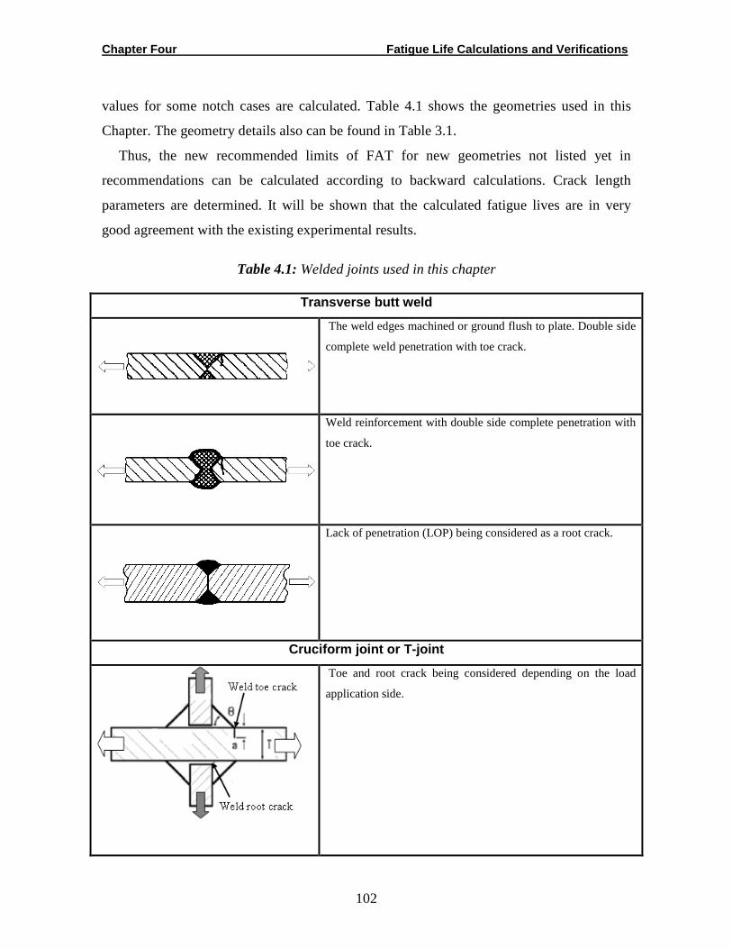
Chapter Four Fatigue Life Calculations and Verifications
102
values for some notch cases are calculated. Table 4.1 shows the geometries used in this
Chapter. The geometry details also can be found in Table 3.1.
Thus, the new recommended limits of FAT for new geometries not listed yet in
recommendations can be calculated according to backward calculations. Crack length
parameters are determined. It will be shown that the calculated fatigue lives are in very
good agreement with the existing experimental results.
Table 4.1: Welded joints used in this chapter
Transverse butt weld
The weld edges machined or ground flush to plate. Double side
complete weld penetration with toe crack.
Weld reinforcement with double side complete penetration with
toe crack.
Lack of penetration (LOP) being considered as a root crack.
Cruciform joint or T-joint
Toe and root crack being considered depending on the load
application side.
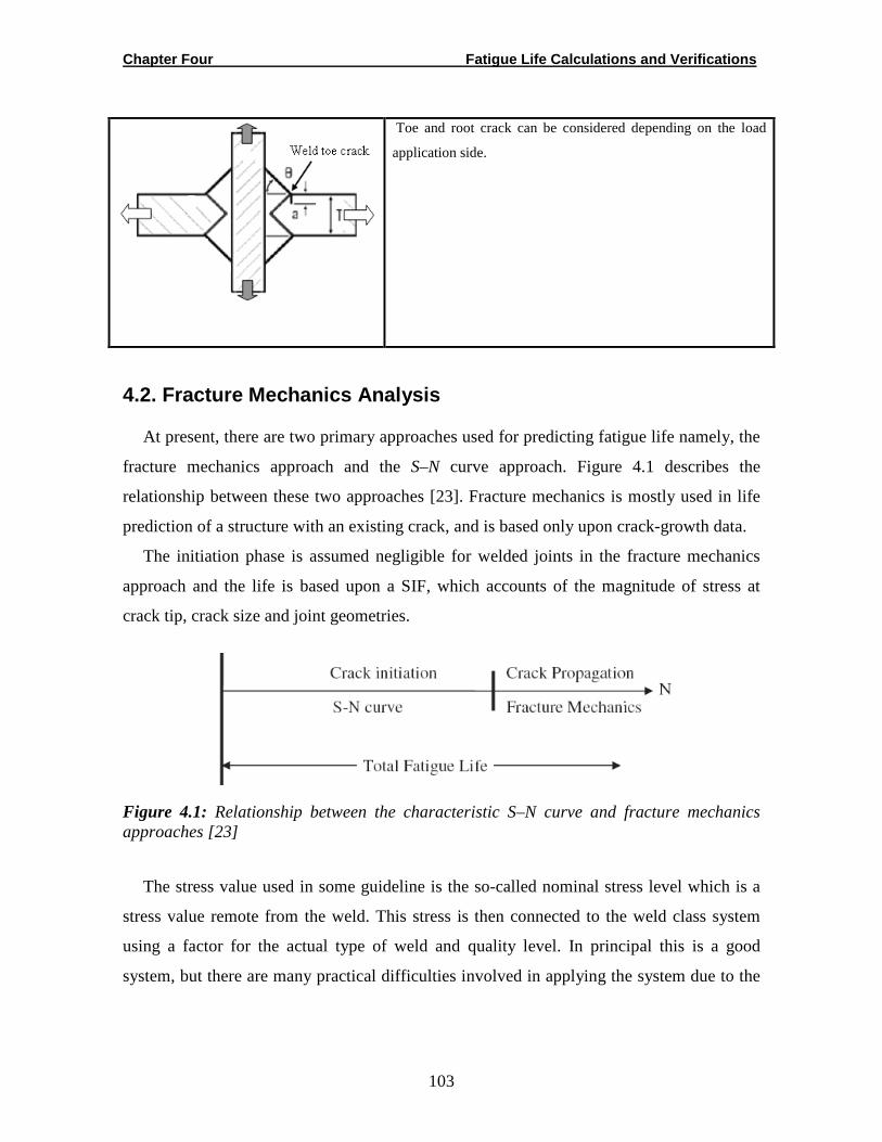
Chapter Four Fatigue Life Calculations and Verifications
103
Toe and root crack can be considered depending on the load
application side.
4.2. Fracture Mechanics Analysis
At present, there are two primary approaches used for predicting fatigue life namely, the
fracture mechanics approach and the S–N curve approach. Figure 4.1 describes the
relationship between these two approaches [23]. Fracture mechanics is mostly used in life
prediction of a structure with an existing crack, and is based only upon crack-growth data.
The initiation phase is assumed negligible for welded joints in the fracture mechanics
approach and the life is based upon a SIF, which accounts of the magnitude of stress at
crack tip, crack size and joint geometries.
Figure 4.1: Relationship between the characteristic S–N curve and fracture mechanics approaches [23]
The stress value used in some guideline is the so-called nominal stress level which is a
stress value remote from the weld. This stress is then connected to the weld class system
using a factor for the actual type of weld and quality level. In principal this is a good
system, but there are many practical difficulties involved in applying the system due to the
Chapter Four Fatigue Life Calculations and Verifications
104
difficulties and impossibilities to define in complex structures, where many points for stress
concentrations and different loading conditions are present [32, 36].
For complex welded structures with many attachments and loads, fracture mechanics
based methods can be used to determine fatigue strength of an unknown notch case of
welded connections. The actual weld toe geometry is considered and an initial crack is
assumed. Moreover, the S-N model cannot deal with the presence of cracks; therefore,
fracture mechanics is an indispensable tool in situations where a crack is detected and sized
[1].
Finally, to be able to use the nominal stress method, the current structure must be
similar to one of the structures available for the method. Misalignments and defects must
lie within the weld class, which means the nominal stress method is only applicable to the
toe side of the weld, and the root side of the weld is frequently neglected in the design
process [36]. In case of welded root cracking, it is usually not possible to measure the stress
in the vicinity of the initiation point since the crack initiation location is embedded inside
the weld [94].
All the above mentioned drawbacks using the nominal stress method in design can be
avoided if local methods are being used. There are at least two such methods: the so called
effective notch method and linear fracture mechanics, which both have proven to work
well. In these methods, the results are taken in direct connection to the weld and all
drawbacks in the nominal method are avoided [32, 36].
The above-mentioned local methods are typically more accurate than the nominal stress
method, especially as the geometric complexity of a structure increases.
4.3. Fatigue Life Calculations Using Paris’ Law
Several equations are proposed by different researchers, usually semi- or wholly-
empirical, to correlate fatigue crack growth rate data with the range of the single parameter
∆K, the range of SIF. Among the proposed equations, Paris–Erdogan relationship is
commonly accepted and used in practice for a wide range of mode-I crack [77]. This
equation is also recommended by IIW to calculate fatigue life for steel and aluminium
welded joints and is still in use today for many applications:
Chapter Four Fatigue Life Calculations and Verifications
105
( )mIKC
dN
da ∆= (4.1)
where da/dN is the crack growth rate per cycle, C and m are material constants determined
from a curve fit (da/dN-∆K curve) to the test data, and ∆KI is the range of the SIF opening
mode [15]. The SIF will be calculated from a FEA as described in the previous chapter.
Paris’ law can be used when it is known that the welding process introduces inherent
surface crack-like flaws at the weld toe, i.e., along the fusion lines when these lines are
brittle and at the weld root. These flaws are regarded as initiated cracks, which is a
somewhat conservative assumption [31].
The calculated fatigue lives are compared with the real experimental test results. In
addition, a fracture mechanics analysis based on accepted standards is done as a reference.
With this local stress fracture mechanics approach, Paris’ equation can be used to
appropriately predict the fatigue crack propagation Np and fatigue life NT of a welded
structure.
The total life NT of a welded joint consists of two phases, namely the crack initiation life
NI and the crack propagation life NP, where the initial crack grows to a certain point and
affects the safety of the structure.
Furthermore, crack initiation in fracture mechanics is defined as a number of cycles that
cause a certain length of crack. Hence, because of welded joints may contain inherent
crack-like defects, discontinuities and stress concentration points, the crack initiation life is
assumed to be negligible.
In this work the determination of the number of cycles N until failure is done by
integration for the crack growth relation from the initial crack depth (ai) up to reaching a
critical crack depth at break-through (af) with the use of the Paris-Erdogan equation:
∫ ∫ ∆=⇒
∆=
N a
am
Im
I
f
iKC
dadN
KC
dadN
0 )()( (4.2)
The SIF range inside is:
aYK I πσ∆=∆ (4.3)
Chapter Four Fatigue Life Calculations and Verifications
106
where ∆σ is the applied stress range, a is the crack length, and Y is the correction factor
mentioned in Chapter Three as a function of f(a/t).
∫ ∫
∆
=N a
am
f
i aY
da
CdN
02
1
)(
1
πσ
(4.4)
Thus, the number of cycles for one increment is:
21)(
1)
21()
21(
1
2m
aa
CY
N
m
i
m
i
mmm −
−
∆=
−−+
πσ (4.5)
In the above equations, the geometry factor Y is assumed as constant, since the inclusion
of a function of (a/t) within the integral sign will usually lead to a formulation that cannot
be integrated analytically. Moreover, the integration cannot be performed directly since the
geometrical factor changes with a. Therefore, to calculate the geometry factor Y in the
above formulas, the SIF has to be evaluated. This is done numerically by using the FEM.
Then, according to SIF, the number of cycles N can be calculated for different loads.
Paris’ equation (Eq. 4.1), which is used to calculate fatigue life in FRANC2D, is very
simple and may not be appropriate for some materials, nonzero load ratios, and very high or
very low SIF ranges. Moreover, the simple application of Paris’ equation does not take into
account the effects of residual stresses and crack closure, where the latter effects are being
included within the stress ratio R. Thus, in many cases, it is more appropriate to calculate
the extract SIF vs. crack length history within FRANC2D, and use this information with a
more sophisticated growth model [78, 79].
Then, other growth equations can be used as Forman, Walker and NASGRO. Finally,
the addition of the crack closure phenomenon to Paris’ model is successfully solved.
In practice, Paris’ law is more straightforward and very often sufficiently accurate to
solve the fatigue life equation by splitting the crack growth history into a series of crack
increments (∆a) in which ∆a is determined according to the stability of the a-N curve.
Chapter Four Fatigue Life Calculations and Verifications
107
Through dividing the crack path into (n) increments, between the initial size ai and the
final size af, then the number of cycles Nj for each increment (between the size aj and the
size aj+∆a) can be calculated. The crack length vector and calculated SIF are transferred to
Excel and integrated numerically according to Eq. (4.2). Then, the total life N can be
calculated by summation of the Nj for each increment as:
( )∑ ∑= = ∆
∆==n
j
n
jm
jI
jKC
aNN
1 1
(4.6)
where j is the steps number. Thus, a numerical integration for a crack growth rate is carried
out at various stress levels, and the results of fatigue life are recorded to determine the S-N
curve. This original model (Model-A) is still used today for many applications.
More advanced models essentially build on the Paris’ equation by addressing mean
stress effects, threshold behavior (Region-I) of da/dN-∆K curve, the instability asymptote
(Region-III), and fatigue crack closure effects. The NASGRO equation is a full range
model that mathematically includes all three regions of FCG curve (Model-B).
4.4. Fatigue Life Calculation Using NASGRO Equation
The superposition method originally is based on the principle of LEFM [65]. Under the
cyclic load and residual stresses, the SIF range and stress ratio are calculated as:
( ) ( ) appminmaxresmin,appresmax,app KKKKKKKK ∆=−=+−+=∆ (4.7)
( ) ( )resmax,appresmin,appres KKKKR ++= (4.8)
Therefore, under cyclic loads, only Rres changes due to the presence of residual stresses.
Considering the welding residual stress effect the original NASGRO equation is expressed
as:
q
c
max
p
thn
ESA
K
K
K
K
KR
fC
dN
da
−
∆
∆−
∆
−−=
1
1
11
(4.9)
Chapter Four Fatigue Life Calculations and Verifications
108
where f is Newmans effective stress ratio and ∆Kth is the threshold value of ∆K for a given
applied stress ratio R=Kmin/Kmax. The parameter CESA, and the exponents n, p, q determine
the shape of the da/dN curve. Kmax is the stress intensity factor at the maximum load for a
given R ratio, and Kc is the critical stress intensity factor which relates to the thickness of
the specimens; more details can be found elsewhere [95].
The solutions, then, use implemented SIF solutions (FEM) and crack growth concepts to
propagate the crack until failure occurs. The Newman’s equation for f is defined as:
3,
2,,, RARARAAf n3n2n1n0 +++= (4.10a)
For R≥0, and for –1≤R<0 as;
RAAf n1n0 ,, += (4.10b)
The polynomial coefficients are defined as:
( ) α
σπαα1
2, /
2cos05.034.0825.0
+−= 0maxn0 SA (4.11a)
( ) 0maxn SA σα /071.0415.0,1 −= (4.11b)
nnn0n AAAA ,3,1,,2 1 −−−= (4.11c)
12 ,1,,3 −+= nn0n AAA (4.11d)
where α is a material constant, its value varies form 1 for plane stress to 3 for plane stain;
Smax is the peak stress of a stress cycle, and σ0 is the material flow stress (i.e., the average of
the tensile yield and ultimate strengths) [96].
NASGRO equation incorporates fatigue crack closure analysis for calculating the effect
of the stress ratio on the crack growth rate under constant amplitude loading.
The threshold stress intensity factor range in Eq. (4.9), ∆Kth, is approximated as a
function of the stress ratio, R, the Newman’s closure function f, the threshold stress
Chapter Four Fatigue Life Calculations and Verifications
109
intensity factor range at R = 0, ∆K0, the crack length, a, and an intrinsic crack length, a0, by
the following empirical equation:
( )( )( )RC
000th
th
RA
f
aa
aKK
+
−−−
+∆=∆
121
11
1/ (4.12)
The values of Cth and ∆K0 are stored as constants in the NASGRO materials files, and a0
has been assigned a fixed value of 0.0015 in. (0.0381 mm). The materials data necessary
for the used materials are obtained from AFGROW database [97] and Ref. [98] (see Table
5.1 of Chapter Five). The SIF due to maximum applied load is defined as:
( )R
KKmax −
∆=1
(4.13)
where ∆K varies between ∆Kth and Kmax.
The current calculation using Model-B becomes more complex for structures which
have the distributions of residual stresses. The use of NASGRO equation under the effect of
residual stresses (Model-C) will be discussed in the next chapter.
4.5. Parameters of Crack Propagation Life
The problem that arises to determine the fatigue life is to choose the appropriate
parameters of C, m, ai, and af. Some studies have presented a range of length for these
crack-like defects in welded joints, and they have given conservative values of lives. Due to
the complex joint geometry, a number of stress concentration points and heterogeneities of
weld metal properties exist in addition to the effect of residual stresses.
The accurate crack lengths and growth parameters have not been established yet. And
this is one of the purposes for the present work.
Traditionally, the fatigue design of welded joints for structural applications has used the
S-N curve type of approach based on experimental results for different weld geometries
[54], included for example in Eurocode 3, BSI7910, BS5400, BS7608 [12, 14, 75, 76] and
IIW [3, 34] where the initial crack length is non-measurable yet and no guidance is found.
However, initial cracks used in fatigue analyses are often in the range of 0.05–0.2 mm [29].
Chapter Four Fatigue Life Calculations and Verifications
110
Nevertheless, these values can vary depending on the welding operation parameters,
geometry and materials properties.
Engesvik [30] has also analyzed the fatigue life of welded joints and concluded that it
may be dubious to apply LEFM at crack depths less than 0.1 mm. In other literature, ai is
usually measured or approximated to 0.1-0.2 mm for welds [31].
BS7910 [14] recommended the initial flaw size, ai between 0.1 and 0.25 mm. The life is
assumed to be finished when the final crack, af reaches one-half of the sheet thickness [31,
32]. Therefore, in this work, trails are carried out to clamp down on bogus sizes of ai and af.
The parameters ai, and af are determined when the C, and m were fixed. Moreover, the
actual weld toe geometry is considered and an initial crack is calculated.
4.6. Selection of the Notch Cases
Cruciform and butt welded joints are the most used geometries in engineering structures.
The factors that presently inhibit the full use of cruciform components are the lack of
standard and suitable specimen design. This aspect is now being addressed through FEM
program with help of fracture mechanics approach through this work to find the values of
the fatigue life and initial crack depths for cruciform weld geometries. The new
recommended limits of FAT and initial crack growth parameter are calculated.
There are two locations of crack initiation that exist at cruciform joints with fillet welds,
at the weld toe, transition between weld and plate, and at the weld root, see Figure 4.2. The
first crack will propagate through the base plate, whereas the second one will propagate
through the weld throat [3, 33].
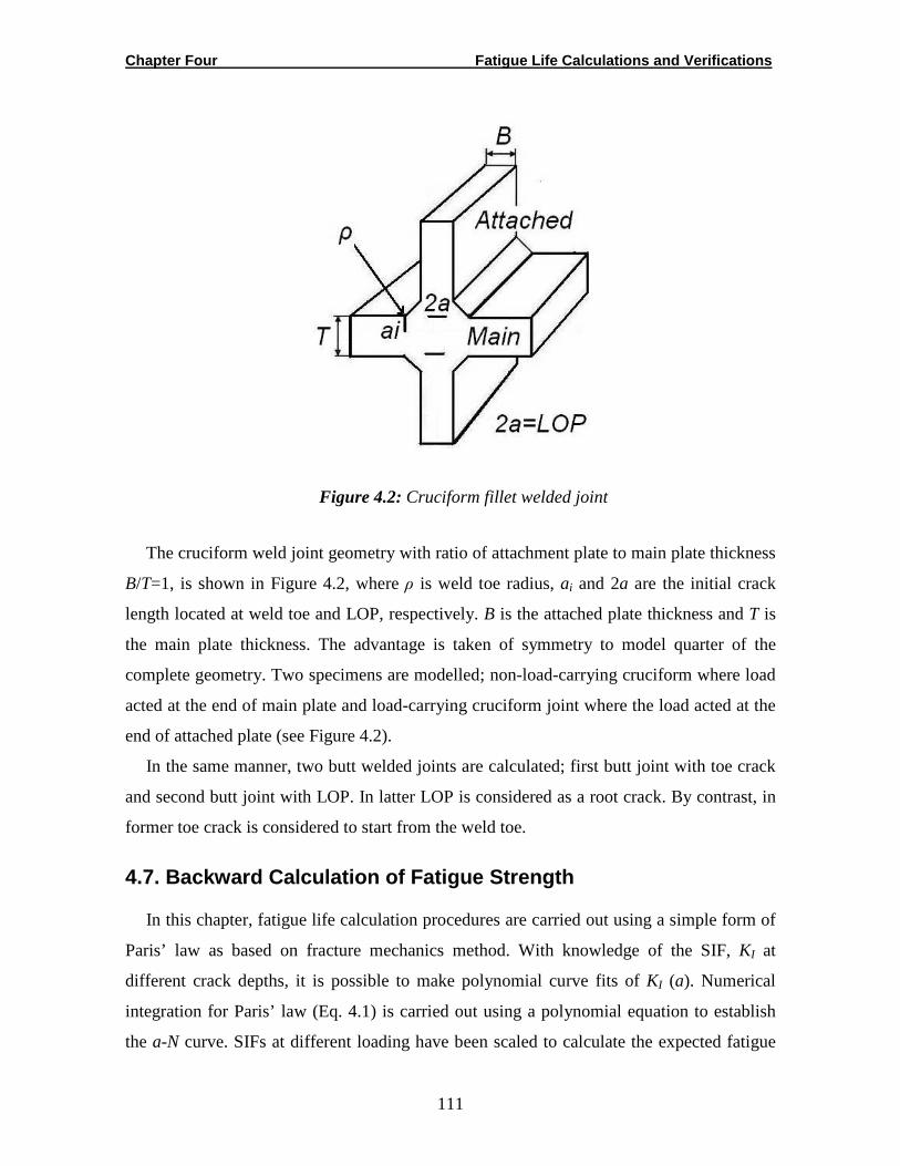
Chapter Four Fatigue Life Calculations and Verifications
111
Figure 4.2: Cruciform fillet welded joint
The cruciform weld joint geometry with ratio of attachment plate to main plate thickness
B/T=1, is shown in Figure 4.2, where ρ is weld toe radius, ai and 2a are the initial crack
length located at weld toe and LOP, respectively. B is the attached plate thickness and T is
the main plate thickness. The advantage is taken of symmetry to model quarter of the
complete geometry. Two specimens are modelled; non-load-carrying cruciform where load
acted at the end of main plate and load-carrying cruciform joint where the load acted at the
end of attached plate (see Figure 4.2).
In the same manner, two butt welded joints are calculated; first butt joint with toe crack
and second butt joint with LOP. In latter LOP is considered as a root crack. By contrast, in
former toe crack is considered to start from the weld toe.
4.7. Backward Calculation of Fatigue Strength
In this chapter, fatigue life calculation procedures are carried out using a simple form of
Paris’ law as based on fracture mechanics method. With knowledge of the SIF, KI at
different crack depths, it is possible to make polynomial curve fits of KI (a). Numerical
integration for Paris’ law (Eq. 4.1) is carried out using a polynomial equation to establish
the a-N curve. SIFs at different loading have been scaled to calculate the expected fatigue

Chapter Four Fatigue Life Calculations and Verifications
112
life for different stress ranges and to develop the S-N curve. A FORTRAN language
program is developed to carry out the numerical integration of Paris’ law at various stress
ranges. The initial crack length is changed to get characteristic and mean FAT values. In
this work, these calculations are referred to Model-A.
If the correct constants for steel (DOMEX 550 MC, high-strength hot rolled steel with
the minimum yield strength 550 MPa and the tensile strength minimum 600 MPa and
maximum 760 MPa, respectively) were not available, the BSI7910 [14] and IIW [3, 34]
recommendations were used, as shown in Table 4.2.
Table 4.2: Characteristic values of recommended materials parameters for steel. Units used are in N and mm
BSI 7910 IIW
C95%=5.21×10⁻¹³, and m=3
C95%=5×10–13, and m=3
Most of fatigue results are distributed and scattered around the mean life value and
further away. If these data are plotted, it will have a bell-shaped curved. The standard
deviation (STDV) is given for data that are distributed normally. According to IIW, all
fatigue resistance data (FAT values) are given as characteristic values, which are assumed
to have a survival probability (reliability) of at least 95% (i.e., 5% failure probability)
within two standard deviations equal to 0.178 calculated from the mean value of a two-
sided 75% confidence level [3]. The initial crack length should be considered in
determination of fatigue life of welded joints. Emphasis is laid on how to choose initial
crack length, ai with the fixed crack growth parameters (C, and m). With the backward
calculations the initial crack length value has been determined which coalescence with the
FAT95% according to characteristic value of C and m. In case of FAT50%, a new value of
C50% is needed to be determined, which is equal to C95%±2STDV. Both curves of these
FAT values are plotted, as shown in Figure 4.3, using the straight line equation with slop m,
i.e.,:
Chapter Four Fatigue Life Calculations and Verifications
113
mLogFATLogCLogN −= (4.14)
Then the characteristic fatigue strength FAT95% is calculated by:
FAT95%: %95%95)102( 6 mLogFATLogCLog −=× (4.14.1)
The mean fatigue strength FAT50% is then:
FAT50%: %50)2%95()102( 6 mLogFATSTDVCLogLog −×+=× (4.14.2)
Finally, the S-N curves are obtained (see Figure 4.3) according to:
)102()/%95( 6××∆= mFATN σ (4.15)
)102()/%50( 6××∆= mFATN σ (4.16)
The mean values of materials constants calculated in this work are given in Table 4.3 for
steel (DOMEX 550 MC steel [31]). The value of C50% is only 8.5% larger than that from
BSI 7910 which is given equal to 2E–13 [14]. These values can be used to calculate
FAT50% for new notch cases.
Table 4.3: Mean values of recommended materials parameters for steel. Units used are in N and mm
According to the current procedures using Model-A (backward calculations), the crack
length value is changed just to fit the curve of FAT95% which is plotted using Eq. (4.15),
as shown in Figure 4.3. Then, these determined values (C, m) from Table 4.1 and initial
crack length from the backward calculations can be used to find FAT95% for new notch
cases which have the same crack classifications (weld toe or weld root crack). Curve of
BSI 7910 Current work
C50%=2×10–13, and m=3
C50%=2.17×10 –13, and m=3
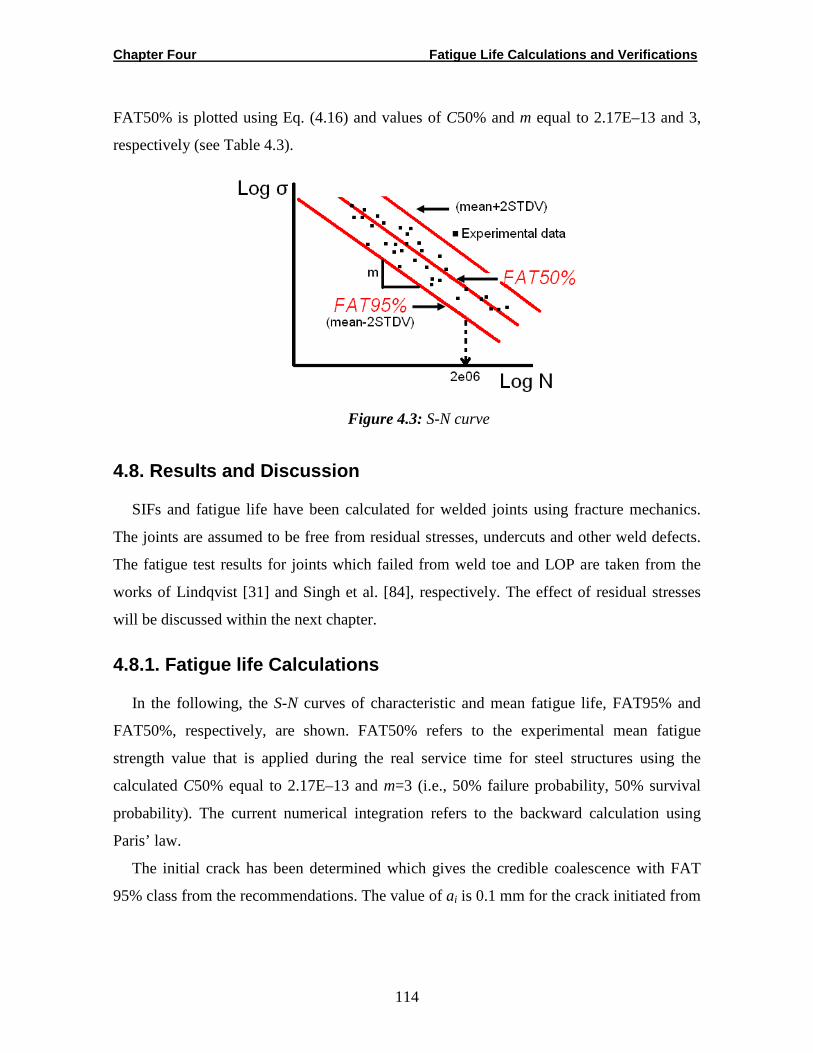
Chapter Four Fatigue Life Calculations and Verifications
114
FAT50% is plotted using Eq. (4.16) and values of C50% and m equal to 2.17E–13 and 3,
respectively (see Table 4.3).
Figure 4.3: S-N curve
4.8. Results and Discussion
SIFs and fatigue life have been calculated for welded joints using fracture mechanics.
The joints are assumed to be free from residual stresses, undercuts and other weld defects.
The fatigue test results for joints which failed from weld toe and LOP are taken from the
works of Lindqvist [31] and Singh et al. [84], respectively. The effect of residual stresses
will be discussed within the next chapter.
4.8.1. Fatigue life Calculations
In the following, the S-N curves of characteristic and mean fatigue life, FAT95% and
FAT50%, respectively, are shown. FAT50% refers to the experimental mean fatigue
strength value that is applied during the real service time for steel structures using the
calculated C50% equal to 2.17E–13 and m=3 (i.e., 50% failure probability, 50% survival
probability). The current numerical integration refers to the backward calculation using
Paris’ law.
The initial crack has been determined which gives the credible coalescence with FAT
95% class from the recommendations. The value of ai is 0.1 mm for the crack initiated from
Chapter Four Fatigue Life Calculations and Verifications
115
the weld toe, while ai is equal to the un-penetrated line for the joints having LOP or
incomplete melting.
To verify the current calculations (Model-A), the results are then compared with
experimental data. It is found that these initial crack lengths of each case are uniform and
have been confirmed for all types of joints. In contrast, final cracks defined in many
researches to be equal to one-half of the parts thickness. In case of LOP, the af was set to be
0.8× (leg length on attached plate side) + (attached plate thickness)/2. The coefficient
multiplying leg length is varied between 0.6 and 0.9 [49]. In all cases, af has a less
significant effect on the fatigue life [31, 40], and the variation can be considered as
negligible.
4.8.1.1. Cruciform Weld Joints having Toe Crack
To determine fatigue life curves for the particular weld details, various standard groups
are put together into categories with similar fatigue behaviour. The compiled results are
from fatigue life testes in several large experimental investigations carried out in Europe,
where the applied stress ranges are in the region of 80 to 105 MPa and the thickness of the
plates is from 16 to 38 mm and stress ratio R between 0 and 0.3 [1]. Linqvist [31] tested
experimentally 12 mm non-load-carrying cruciform specimens under tension made of the
steel DOMEX 550 MC, which is an extra high-strength hot rolled steel with minimum yield
strength 550 MPa. The tensile strength is minimum 600 MPa and maximum 760 MPa,
respectively. The weld toe radius is set at 0.6 mm. The model started with the initial crack
ai from the weld toe. The initial crack will grow in depth regularly. The reported test results
are compared with calculated results from backward calculations procedure used in the
current study.
Fatigue life calculation is defined as the stage when the crack has reached its final
length, which is defined in many researches to be equal to one-half of the parts thickness
[31]. In this work, af values equal to one-half of the sheet thickness is adopted. In addition,
these values of af have been verified which give the fix number of cycles in the a-N curve,
i.e when the increase in fatigue life was negligible [15]. Figure 4.4 shows that af is about
5.2 mm in case of sharp weld toe (no radius). The value of af increases to approximately 6
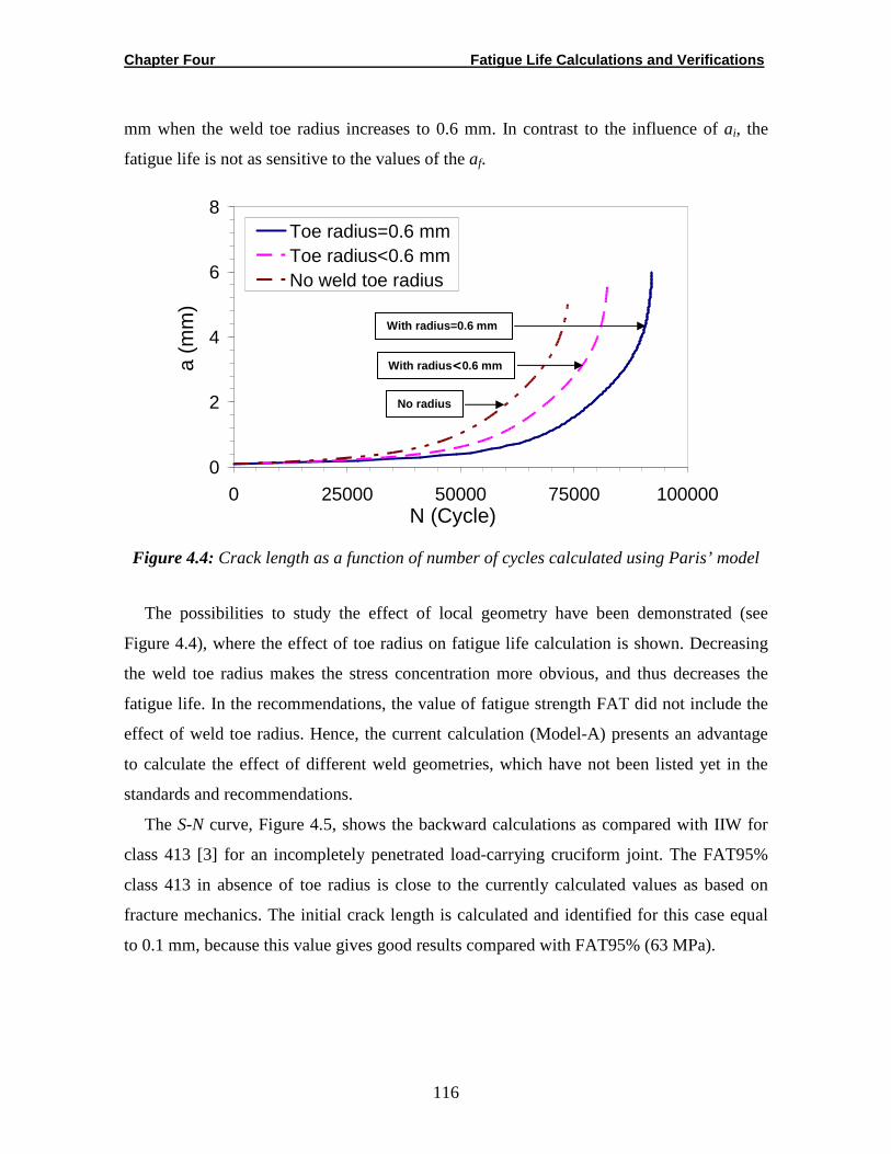
Chapter Four Fatigue Life Calculations and Verifications
116
mm when the weld toe radius increases to 0.6 mm. In contrast to the influence of ai, the
fatigue life is not as sensitive to the values of the af.
0
2
4
6
8
0 25000 50000 75000 100000N (Cycle)
a (m
m)
Toe radius=0.6 mmToe radius<0.6 mmNo weld toe radius
Figure 4.4: Crack length as a function of number of cycles calculated using Paris’ model
The possibilities to study the effect of local geometry have been demonstrated (see
Figure 4.4), where the effect of toe radius on fatigue life calculation is shown. Decreasing
the weld toe radius makes the stress concentration more obvious, and thus decreases the
fatigue life. In the recommendations, the value of fatigue strength FAT did not include the
effect of weld toe radius. Hence, the current calculation (Model-A) presents an advantage
to calculate the effect of different weld geometries, which have not been listed yet in the
standards and recommendations.
The S-N curve, Figure 4.5, shows the backward calculations as compared with IIW for
class 413 [3] for an incompletely penetrated load-carrying cruciform joint. The FAT95%
class 413 in absence of toe radius is close to the currently calculated values as based on
fracture mechanics. The initial crack length is calculated and identified for this case equal
to 0.1 mm, because this value gives good results compared with FAT95% (63 MPa).
No radius
With radius=0.6 mm
With radius <0.6 mm
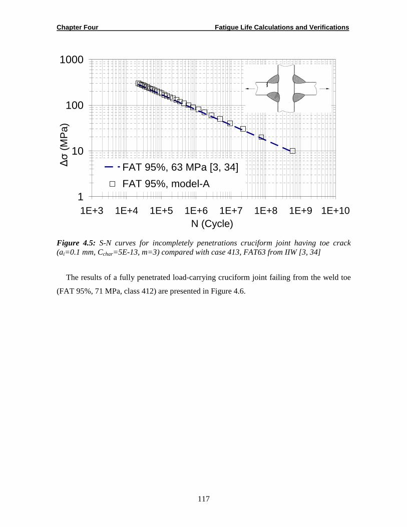
Chapter Four Fatigue Life Calculations and Verifications
117
1
10
100
1000
1E+3 1E+4 1E+5 1E+6 1E+7 1E+8 1E+9 1E+10N (Cycle)
∆σ
(M
Pa)
FAT 95%, 63 MPa [3, 34]
FAT 95%, model-A
Figure 4.5: S-N curves for incompletely penetrations cruciform joint having toe crack (ai=0.1 mm, Cchar=5E-13, m=3) compared with case 413, FAT63 from IIW [3, 34]
The results of a fully penetrated load-carrying cruciform joint failing from the weld toe
(FAT 95%, 71 MPa, class 412) are presented in Figure 4.6.

Chapter Four Fatigue Life Calculations and Verifications
118
1
10
100
1000
1E+3 1E+4 1E+5 1E+6 1E+7 1E+8 1E+9 1E+10N (Cycle)
∆σ
(M
Pa)
FAT 95%, 71 MPa [3, 34]
FAT 95%, model-A
Figure 4.6: S-N curves for full penetration cruciform joint having toe crack (ai=0.1 mm, Cchar=5E-13, m=3) compared with case 412, FAT71 from IIW [3, 34]
From Figures 4.5 and 4.6, it is noticed that the value of initial crack 0.1 mm is creditable
for the case of toe crack in two types of cruciform joints. The currently calculated life is
located between these two lives. The calculated lives, characteristic and mean life
(FAT95% and FAT50%, respectively) are presented in Figure 4.7, in comparison with the
values from IIW.
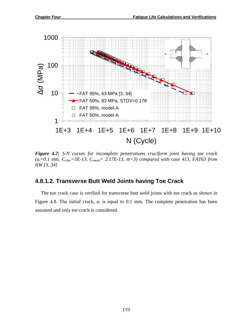
Chapter Four Fatigue Life Calculations and Verifications
119
1
10
100
1000
1E+3 1E+4 1E+5 1E+6 1E+7 1E+8 1E+9 1E+10
N (Cycle)
∆σ
(M
Pa)
FAT 95%, 63 MPa [3, 34]
FAT 50%, 83 MPa, STDV=0.178
FAT 95%, model-A
FAT 50%, model-A
Figure 4.7: S-N curves for incomplete penetrations cruciform joint having toe crack (ai=0.1 mm, Cchar=5E-13, Cmean= 2.17E-13, m=3) compared with case 413, FAT63 from IIW [3, 34]
4.8.1.2. Transverse Butt Weld Joints having Toe Cra ck
The toe crack case is verified for transverse butt weld joints with toe crack as shown in
Figure 4.8. The initial crack, ai is equal to 0.1 mm. The complete penetration has been
assumed and only toe crack is considered.
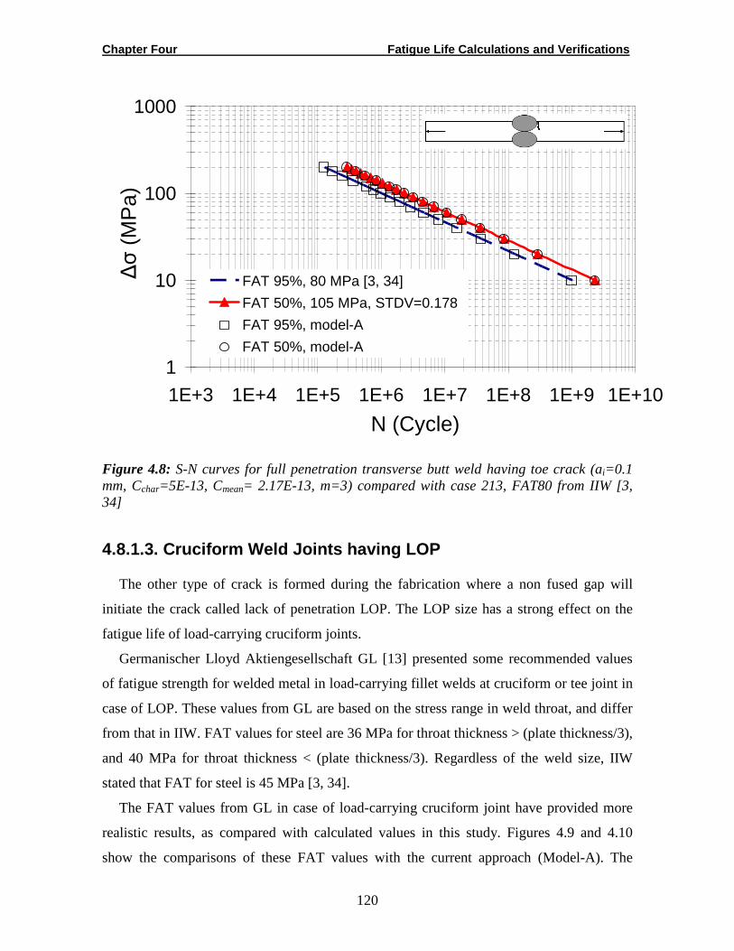
Chapter Four Fatigue Life Calculations and Verifications
120
1
10
100
1000
1E+3 1E+4 1E+5 1E+6 1E+7 1E+8 1E+9 1E+10
N (Cycle)
∆σ
(M
Pa)
FAT 95%, 80 MPa [3, 34]
FAT 50%, 105 MPa, STDV=0.178
FAT 95%, model-A
FAT 50%, model-A
Figure 4.8: S-N curves for full penetration transverse butt weld having toe crack (ai=0.1 mm, Cchar=5E-13, Cmean= 2.17E-13, m=3) compared with case 213, FAT80 from IIW [3, 34]
4.8.1.3. Cruciform Weld Joints having LOP
The other type of crack is formed during the fabrication where a non fused gap will
initiate the crack called lack of penetration LOP. The LOP size has a strong effect on the
fatigue life of load-carrying cruciform joints.
Germanischer Lloyd Aktiengesellschaft GL [13] presented some recommended values
of fatigue strength for welded metal in load-carrying fillet welds at cruciform or tee joint in
case of LOP. These values from GL are based on the stress range in weld throat, and differ
from that in IIW. FAT values for steel are 36 MPa for throat thickness > (plate thickness/3),
and 40 MPa for throat thickness < (plate thickness/3). Regardless of the weld size, IIW
stated that FAT for steel is 45 MPa [3, 34].
The FAT values from GL in case of load-carrying cruciform joint have provided more
realistic results, as compared with calculated values in this study. Figures 4.9 and 4.10
show the comparisons of these FAT values with the current approach (Model-A). The

Chapter Four Fatigue Life Calculations and Verifications
121
fatigue strength increases with a decrease of weld size (throat thickness) due to the effect of
the stress concentration.
1
10
100
1000
1E+3 1E+4 1E+5 1E+6 1E+7 1E+8 1E+9 1E+10
N (Cycle)
∆σ
(M
Pa)
FAT 95%, 36 MPa [13]FAT 50%, 47 MPa, STDV=0.178 FAT 95%, model-AFAT 50%, model-A
Figure 4.9: S-N curves for incomplete penetration cruciform joint having LOP (2ai=LOP=7 mm, Cchar=5E-13, Cmean= 2.17E-13, m=3 and throat thick>t/3) compared with type No. 23, FAT36 from GL [13]
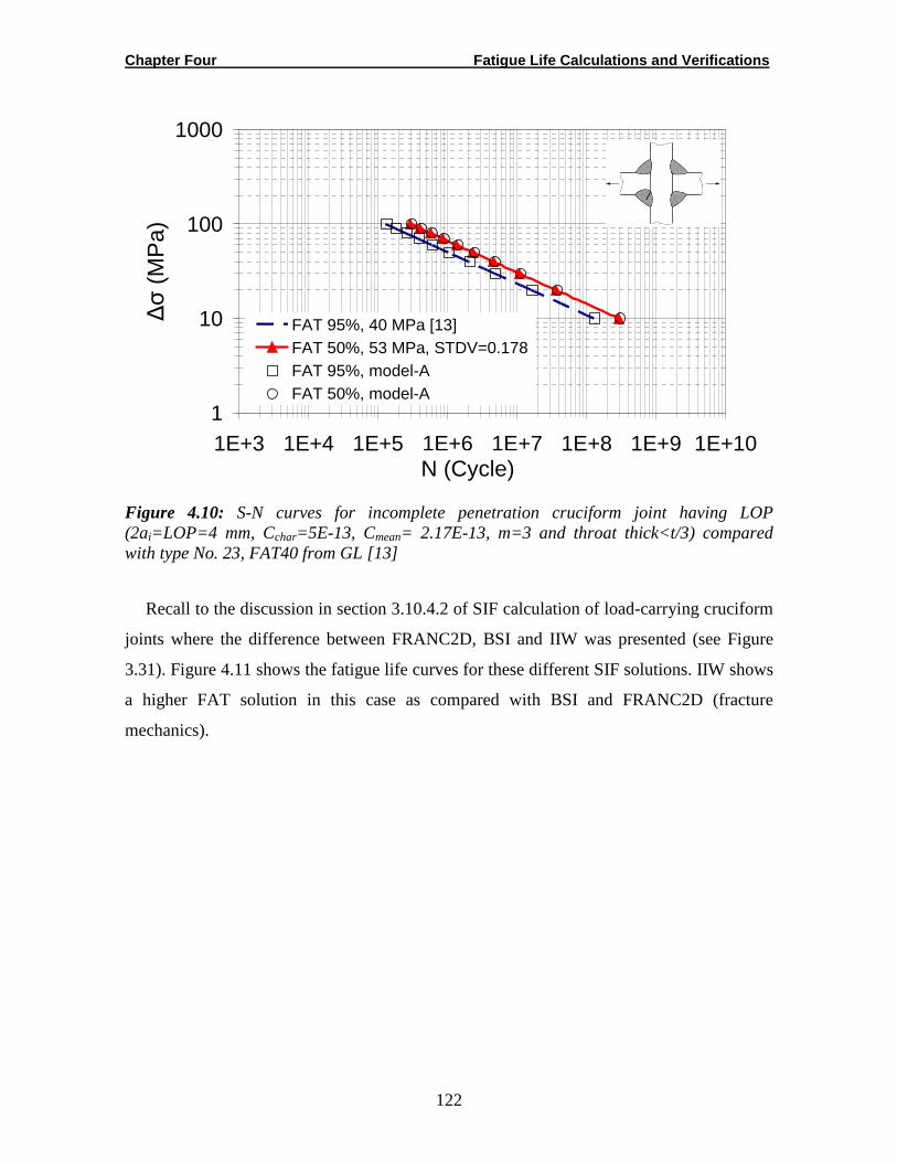
Chapter Four Fatigue Life Calculations and Verifications
122
1
10
100
1000
1E+3 1E+4 1E+5 1E+6 1E+7 1E+8 1E+9 1E+10N (Cycle)
∆σ
(M
Pa)
FAT 95%, 40 MPa [13]FAT 50%, 53 MPa, STDV=0.178FAT 95%, model-AFAT 50%, model-A
Figure 4.10: S-N curves for incomplete penetration cruciform joint having LOP (2ai=LOP=4 mm, Cchar=5E-13, Cmean= 2.17E-13, m=3 and throat thick<t/3) compared with type No. 23, FAT40 from GL [13]
Recall to the discussion in section 3.10.4.2 of SIF calculation of load-carrying cruciform
joints where the difference between FRANC2D, BSI and IIW was presented (see Figure
3.31). Figure 4.11 shows the fatigue life curves for these different SIF solutions. IIW shows
a higher FAT solution in this case as compared with BSI and FRANC2D (fracture
mechanics).
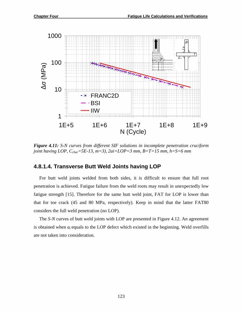
Chapter Four Fatigue Life Calculations and Verifications
123
1
10
100
1000
1E+5 1E+6 1E+7 1E+8 1E+9N (Cycle)
∆σ
(M
Pa)
FRANC2DBSI IIW
Figure 4.11: S-N curves from different SIF solutions in incomplete penetration cruciform joint having LOP, Cchar=5E-13, m=3), 2ai=LOP=3 mm, B=T=15 mm, h=S=6 mm
4.8.1.4. Transverse Butt Weld Joints having LOP
For butt weld joints welded from both sides, it is difficult to ensure that full root
penetration is achieved. Fatigue failure from the weld roots may result in unexpectedly low
fatigue strength [15]. Therefore for the same butt weld joint, FAT for LOP is lower than
that for toe crack (45 and 80 MPa, respectively). Keep in mind that the latter FAT80
considers the full weld penetration (no LOP).
The S-N curves of butt weld joints with LOP are presented in Figure 4.12. An agreement
is obtained when ai equals to the LOP defect which existed in the beginning. Weld overfills
are not taken into consideration.
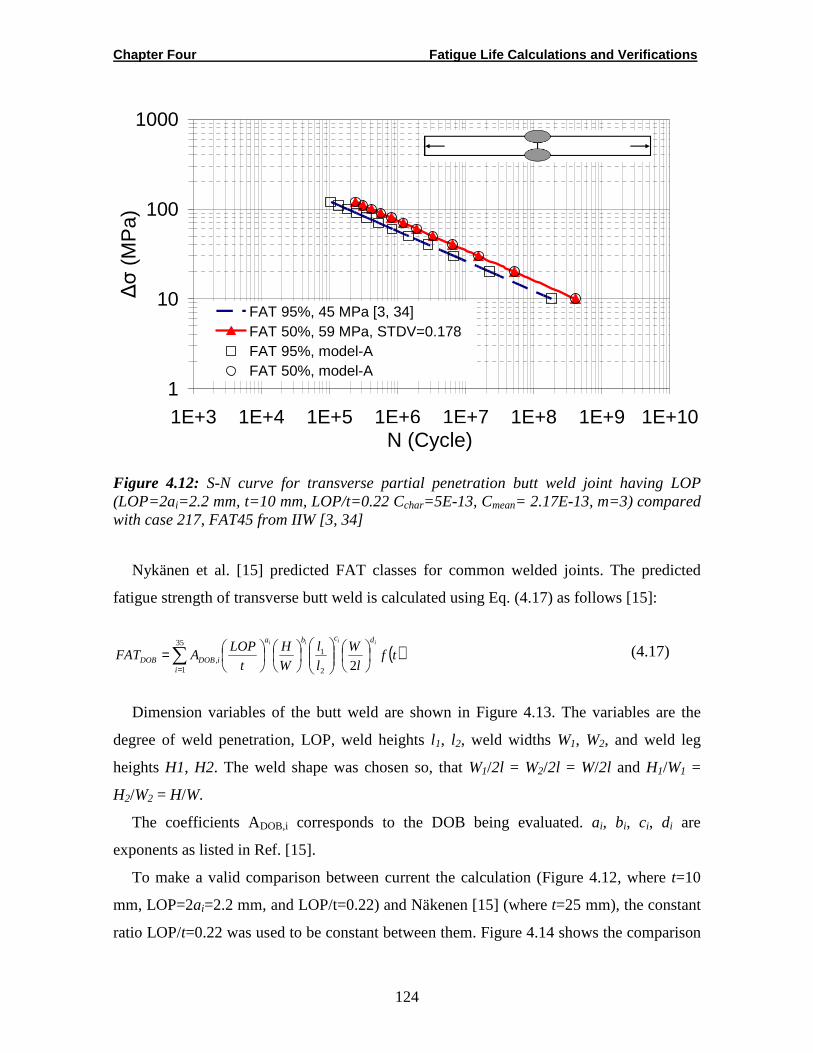
Chapter Four Fatigue Life Calculations and Verifications
124
1
10
100
1000
1E+3 1E+4 1E+5 1E+6 1E+7 1E+8 1E+9 1E+10N (Cycle)
∆σ
(M
Pa)
FAT 95%, 45 MPa [3, 34]FAT 50%, 59 MPa, STDV=0.178FAT 95%, model-AFAT 50%, model-A
Figure 4.12: S-N curve for transverse partial penetration butt weld joint having LOP (LOP=2ai=2.2 mm, t=10 mm, LOP/t=0.22 Cchar=5E-13, Cmean= 2.17E-13, m=3) compared with case 217, FAT45 from IIW [3, 34]
Nykänen et al. [15] predicted FAT classes for common welded joints. The predicted
fatigue strength of transverse butt weld is calculated using Eq. (4.17) as follows [15]:
( )tfl
W
l
l
W
H
t
LOPAFAT
iiii dcba
iiDOBDOB
=∑= 22
135
1,
(4.17)
Dimension variables of the butt weld are shown in Figure 4.13. The variables are the
degree of weld penetration, LOP, weld heights l1, l2, weld widths W1, W2, and weld leg
heights H1, H2. The weld shape was chosen so, that W1/2l = W2/2l = W/2l and H1/W1 =
H2/W2 = H/W.
The coefficients ADOB,i corresponds to the DOB being evaluated. ai, bi, ci, di are
exponents as listed in Ref. [15].
To make a valid comparison between current the calculation (Figure 4.12, where t=10
mm, LOP=2ai=2.2 mm, and LOP/t=0.22) and Näkenen [15] (where t=25 mm), the constant
ratio LOP/t=0.22 was used to be constant between them. Figure 4.14 shows the comparison
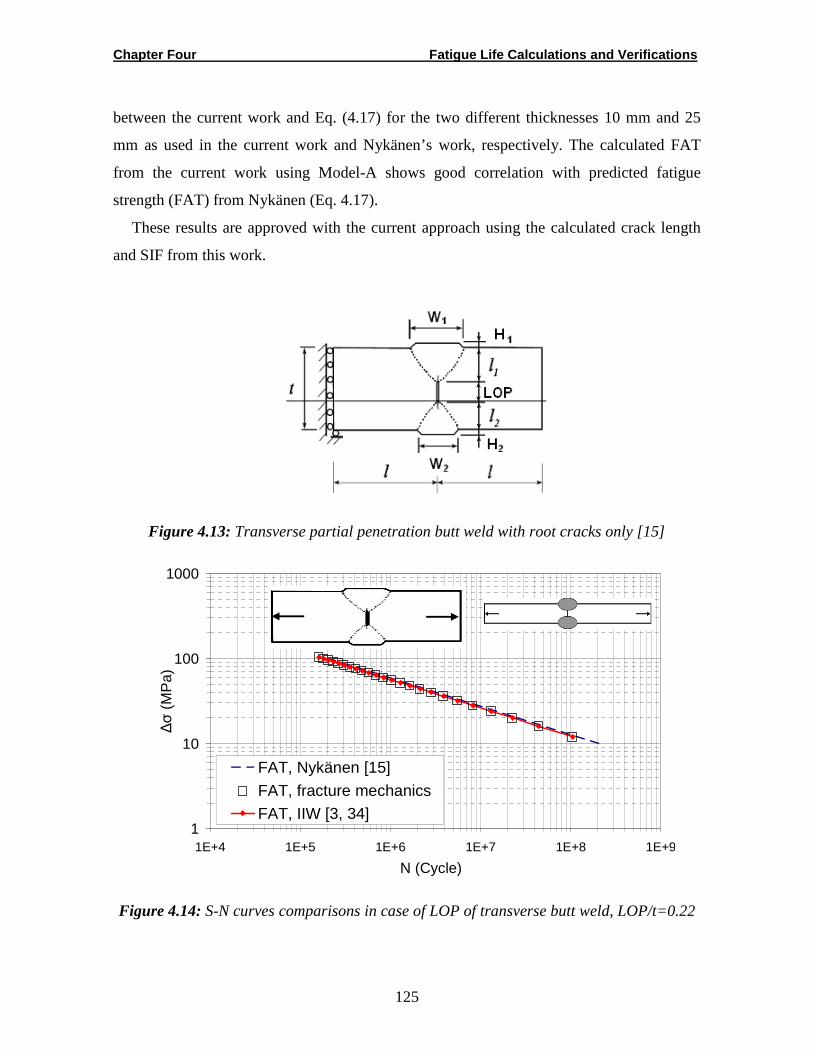
Chapter Four Fatigue Life Calculations and Verifications
125
between the current work and Eq. (4.17) for the two different thicknesses 10 mm and 25
mm as used in the current work and Nykänen’s work, respectively. The calculated FAT
from the current work using Model-A shows good correlation with predicted fatigue
strength (FAT) from Nykänen (Eq. 4.17).
These results are approved with the current approach using the calculated crack length
and SIF from this work.
Figure 4.13: Transverse partial penetration butt weld with root cracks only [15]
1
10
100
1000
1E+4 1E+5 1E+6 1E+7 1E+8 1E+9
N (Cycle)
∆σ
(M
Pa)
FAT, Nykänen [15]
FAT, fracture mechanics
FAT, IIW [3, 34]
Figure 4.14: S-N curves comparisons in case of LOP of transverse butt weld, LOP/t=0.22

Chapter Four Fatigue Life Calculations and Verifications
126
The FE direct simulation for butt weld joint from Nykänen (Figure 4.13) is carried out
using FRANC2D where the thickness=25 mm. Then, SIF was calculated and Eq. (4.18) is
developed to be used in Paris’ numerical integration program.
57.344)(86.100)(708.45)(8122.5)(2914.0 234 +−+−= aaaaK (4.18)
The initial crack equals to the LOP is assumed using Model-A, with Paris’ law constants m
= 3, and Cchar = 3 E-13 (da/dN in mm/cycle and ∆K in Nmm-3/2) as used by Nykänen [15],
the fatigue life curves are presented in Figure 4.15. Good agreement between the two
solutions is shown in this case.
It is to be emphasized that the predicted FAT from Eq. (4.17), are calculated for H/W =
0.1, W/2l = 0.5 and t = 25 mm. This mean that for the unequal weld dimension (W1≠W2,
l1≠l2), Eq. 4.17 is not able to find a corresponding FAT. Therefore the recommendation to
use the current approach (Model-A) with the calculated parameters will take an advantage,
because only SIFs with ai are needed to find an appropriate FAT for different geometries
(see Figure 4.15).
1
10
100
1000
1E+4 1E+5 1E+6 1E+7 1E+8 1E+9
N (Cycle)
∆σ
(M
Pa)
FAT 95%, fracture mechanics
FAT 95%, Nykänen [15]
Figure 4.15: S-N curves using Eq 4.17 and the current approach (Model-A) for LOP of transverse butt weld, thickness=25 mm, 2ai=LOP=5.5 mm, LOP/t=0.22
Chapter Four Fatigue Life Calculations and Verifications
127
4.9. Experimental Verifications
From literature [16, 17, 18], it is evident that most of fatigue life predictions of fillet
welded joints are based on toe failure. Some other studies [20, 22, 84, 92] have considered
the fatigue behaviour of fillet welded cruciform joints failing from the root region.
For fillet welds, the high stress concentration locates at the weld toe due to the fact that
these locations are rarely sound and usually weldment contains flaws, crack-like defects
and stress concentrations. Therefore, the presence of the weld toe radius inevitably will
reduce these concentrations of stresses near the weld toe.
The effect of the toe radius is not included in FAT values from IIW and BSI 7910
recommendations. This will provide a good example to evaluate the current approach
(Model-A) from this work. Lindqvist [31] conducted the fatigue test for toe crack in a non-
load-carrying cruciform weld joint having 0.6 mm toe radius. The reported results are
compared with the current approach (Model-A) under tension mode only.
In this study, the new value of FAT95% for non-load carrying fillet weld having toe
radius have been calculated equal to 71 MPa.
The new calculated FAT value is higher than that from IIW recommendations
(FAT95%, 63 MPa) due to the effect of improved local weld geometries and stress
concentration.
To verify the predicted value, the mean or design curve is drawn as shown in Figure
4.16. The mean curve fatigue life (FAT50%) calculated is based on FAT95%+2STDV.
FAT50% is compared with reported test results from Lindqvist [31]. An initial crack length
equal to 0.1 mm was adopted.
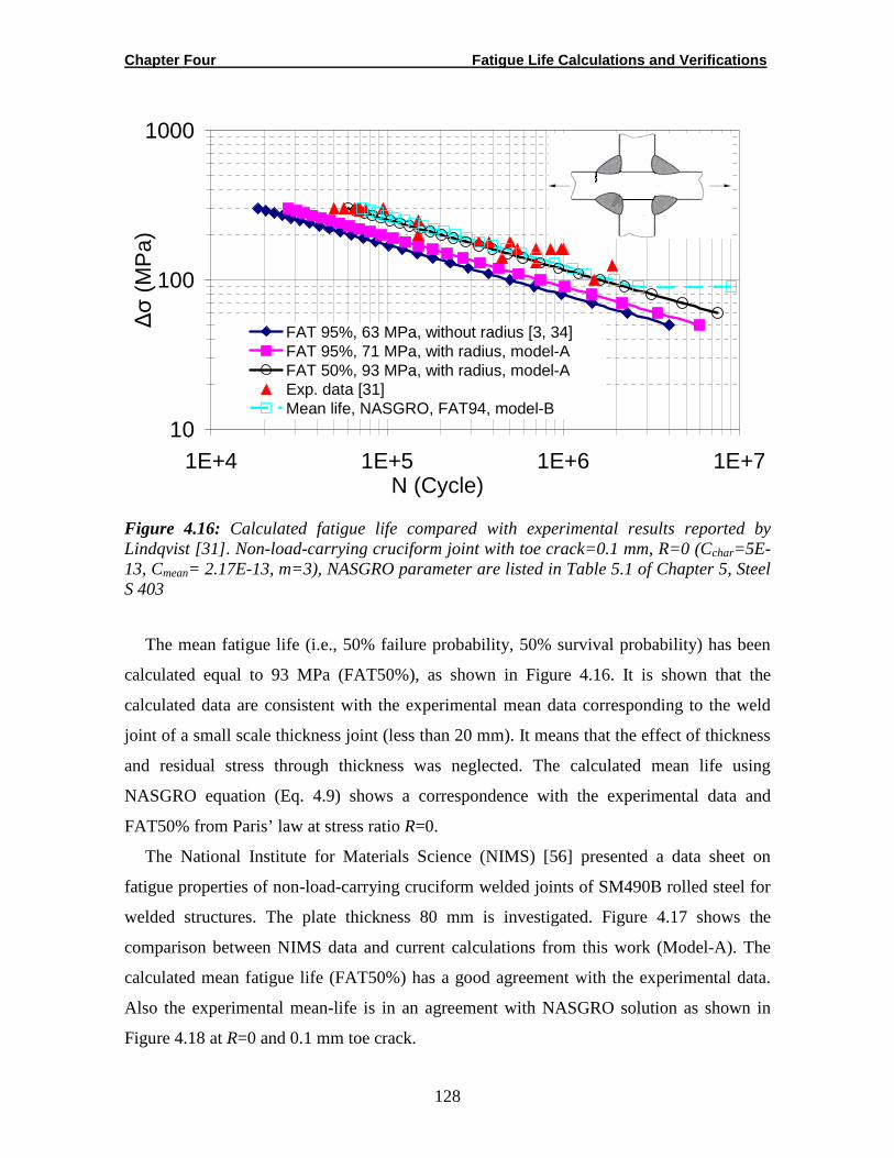
Chapter Four Fatigue Life Calculations and Verifications
128
10
100
1000
1E+4 1E+5 1E+6 1E+7
∆σ
(M
Pa)
FAT 95%, 63 MPa, without radius [3, 34]FAT 95%, 71 MPa, with radius, model-AFAT 50%, 93 MPa, with radius, model-AExp. data [31]Mean life, NASGRO, FAT94, model-B
N (Cycle)
Figure 4.16: Calculated fatigue life compared with experimental results reported by Lindqvist [31]. Non-load-carrying cruciform joint with toe crack=0.1 mm, R=0 (Cchar=5E-13, Cmean= 2.17E-13, m=3), NASGRO parameter are listed in Table 5.1 of Chapter 5, Steel S 403
The mean fatigue life (i.e., 50% failure probability, 50% survival probability) has been
calculated equal to 93 MPa (FAT50%), as shown in Figure 4.16. It is shown that the
calculated data are consistent with the experimental mean data corresponding to the weld
joint of a small scale thickness joint (less than 20 mm). It means that the effect of thickness
and residual stress through thickness was neglected. The calculated mean life using
NASGRO equation (Eq. 4.9) shows a correspondence with the experimental data and
FAT50% from Paris’ law at stress ratio R=0.
The National Institute for Materials Science (NIMS) [56] presented a data sheet on
fatigue properties of non-load-carrying cruciform welded joints of SM490B rolled steel for
welded structures. The plate thickness 80 mm is investigated. Figure 4.17 shows the
comparison between NIMS data and current calculations from this work (Model-A). The
calculated mean fatigue life (FAT50%) has a good agreement with the experimental data.
Also the experimental mean-life is in an agreement with NASGRO solution as shown in
Figure 4.18 at R=0 and 0.1 mm toe crack.
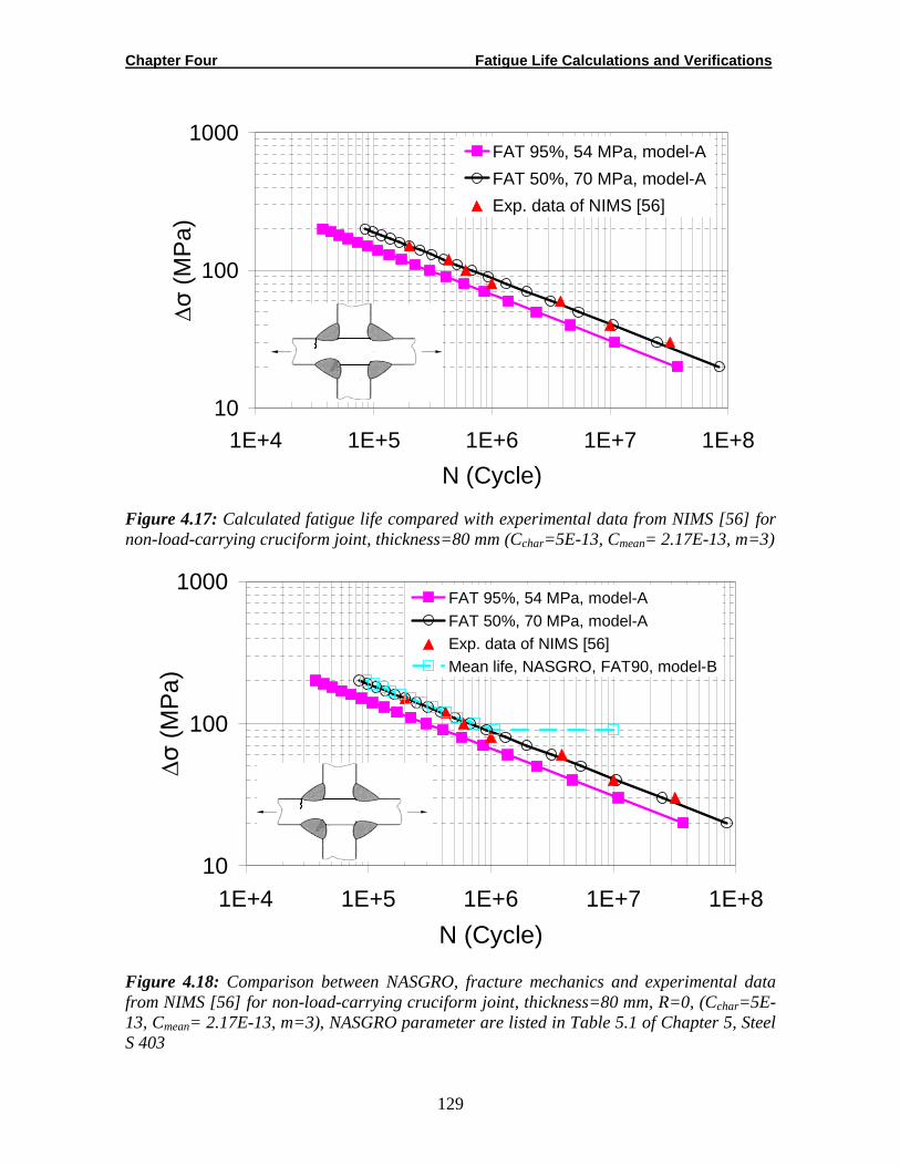
Chapter Four Fatigue Life Calculations and Verifications
129
10
100
1000
1E+4 1E+5 1E+6 1E+7 1E+8
N (Cycle)
∆σ
(M
Pa)
FAT 95%, 54 MPa, model-A
FAT 50%, 70 MPa, model-A
Exp. data of NIMS [56]
Figure 4.17: Calculated fatigue life compared with experimental data from NIMS [56] for non-load-carrying cruciform joint, thickness=80 mm (Cchar=5E-13, Cmean= 2.17E-13, m=3)
10
100
1000
1E+4 1E+5 1E+6 1E+7 1E+8
N (Cycle)
∆σ
(M
Pa)
FAT 95%, 54 MPa, model-AFAT 50%, 70 MPa, model-AExp. data of NIMS [56]Mean life, NASGRO, FAT90, model-B
Figure 4.18: Comparison between NASGRO, fracture mechanics and experimental data from NIMS [56] for non-load-carrying cruciform joint, thickness=80 mm, R=0, (Cchar=5E-13, Cmean= 2.17E-13, m=3), NASGRO parameter are listed in Table 5.1 of Chapter 5, Steel S 403
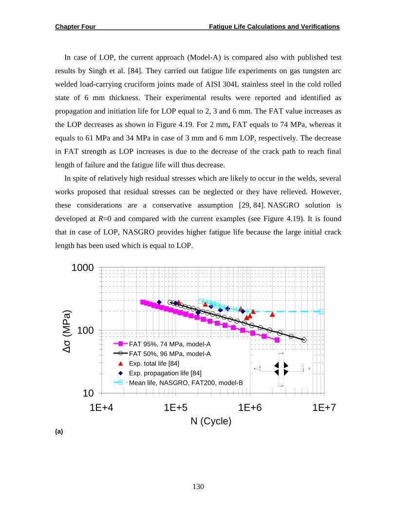
Chapter Four Fatigue Life Calculations and Verifications
130
In case of LOP, the current approach (Model-A) is compared also with published test
results by Singh et al. [84]. They carried out fatigue life experiments on gas tungsten arc
welded load-carrying cruciform joints made of AISI 304L stainless steel in the cold rolled
state of 6 mm thickness. Their experimental results were reported and identified as
propagation and initiation life for LOP equal to 2, 3 and 6 mm. The FAT value increases as
the LOP decreases as shown in Figure 4.19. For 2 mm, FAT equals to 74 MPa, whereas it
equals to 61 MPa and 34 MPa in case of 3 mm and 6 mm LOP, respectively. The decrease
in FAT strength as LOP increases is due to the decrease of the crack path to reach final
length of failure and the fatigue life will thus decrease.
In spite of relatively high residual stresses which are likely to occur in the welds, several
works proposed that residual stresses can be neglected or they have relieved. However,
these considerations are a conservative assumption [29, 84]. NASGRO solution is
developed at R=0 and compared with the current examples (see Figure 4.19). It is found
that in case of LOP, NASGRO provides higher fatigue life because the large initial crack
length has been used which is equal to LOP.
10
100
1000
1E+4 1E+5 1E+6 1E+7N (Cycle)
∆σ
(M
Pa)
FAT 95%, 74 MPa, model-A
FAT 50%, 96 MPa, model-A
Exp. total life [84]
Exp. propagation life [84]
Mean life, NASGRO, FAT200, model-B
(a)

Chapter Four Fatigue Life Calculations and Verifications
131
10
100
1000
1E+4 1E+5 1E+6 1E+7N (Cycle)
∆σ
(M
Pa)
FAT 95%, 61 MPa, model-AFAT 50%, 79 MPa, model-AExp. total life [84]Exp. propagation life [84]Mean life, NASGRO, FAT170, model-B
(b)
10
100
1000
1E+4 1E+5 1E+6 1E+7N (Cycle)
∆σ
(M
Pa)
FAT 95%, 34 MPa, model-AFAT 50%, 44 MPa, model-AExp. total life [84]Exp. propagation life [84]Mean life, NASGRO, FAT100, model-B
(c)
Figure 4.19: Calculated fatigue life based on Paris and NASGRO equations compared with experimental data reported by Singh [84] at R=0, (Cchar=5E-13, Cmean= 2.17E-13, m=3): NASGRO parameter are listed in Table 5.1 of Chapter 5, Steel S 403(a) LOP= 2 mm; (b) LOP=3 mm; (c) LOP=6 mm
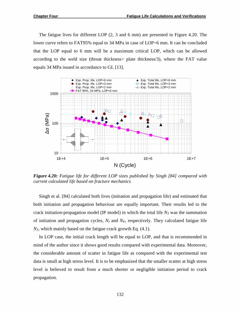
Chapter Four Fatigue Life Calculations and Verifications
132
The fatigue lives for different LOP (2, 3 and 6 mm) are presented in Figure 4.20. The
lower curve refers to FAT95% equal to 34 MPa in case of LOP=6 mm. It can be concluded
that the LOP equal to 6 mm will be a maximum critical LOP, which can be allowed
according to the weld size (throat thickness> plate thickness/3), where the FAT value
equals 34 MPa issued in accordance to GL [13].
10
100
1000
1E+4 1E+5 1E+6 1E+7
N (Cycle)
∆σ
(M
Pa)
Exp. Prop. life, LOP=6 mm Exp. Total life, LOP=6 mmExp. Prop. life, LOP=3 mm Exp. Total life, LOP=3 mmExp. Prop. life, LOP=2 mm Exp. Total life, LOP=2 mmFAT 95%, 34 MPa, LOP=6 mm
Figure 4.20: Fatigue life for different LOP sizes published by Singh [84] compared with current calculated life based on fracture mechanics
Singh et al. [84] calculated both lives (initiation and propagation life) and estimated that
both initiation and propagation behaviour are equally important. Their results led to the
crack initiation-propagation model (IP model) in which the total life NT was the summation
of initiation and propagation cycles, NI and NP, respectively. They calculated fatigue life
NT, which mainly based on the fatigue crack growth Eq. (4.1).
In LOP case, the initial crack length will be equal to LOP, and that is recommended in
mind of the author since it shows good results compared with experimental data. Moreover,
the considerable amount of scatter in fatigue life as compared with the experimental test
data is small at high stress level. It is to be emphasized that the smaller scatter at high stress
level is believed to result from a much shorter or negligible initiation period to crack
propagation.
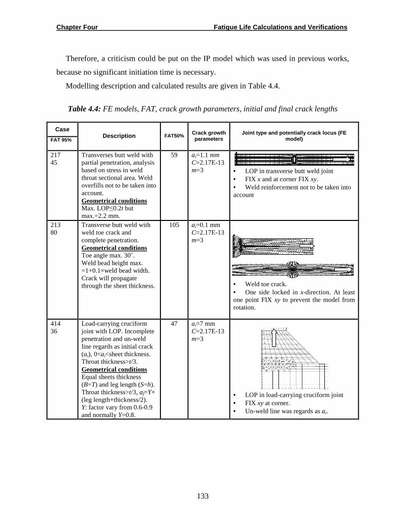
Chapter Four Fatigue Life Calculations and Verifications
133
Therefore, a criticism could be put on the IP model which was used in previous works,
because no significant initiation time is necessary.
Modelling description and calculated results are given in Table 4.4.
Table 4.4: FE models, FAT, crack growth parameters, initial and final crack lengths
Case
FAT 95% Description FAT50% Crack growth
parameters Joint type and potentially crack locus (FE
model)
217 45
Transverses butt weld with partial penetration, analysis based on stress in weld throat sectional area. Weld overfills not to be taken into account. Geometrical conditions Max. LOP≤0.2t but max.=2.2 mm.
59 ai=1.1 mm C=2.17E-13 m=3
• LOP in transverse butt weld joint • FIX x and at corner FIX xy. • Weld reinforcement not to be taken into account
213 80
Transverse butt weld with weld toe crack and complete penetration. Geometrical conditions Toe angle max. 30˚. Weld bead height max. =1+0.1×weld bead width. Crack will propagate through the sheet thickness.
105 ai=0.1 mm C=2.17E-13 m=3
• Weld toe crack. • One side locked in x-direction. At least one point FIX xy to prevent the model from rotation.
414 36
Load-carrying cruciform joint with LOP. Incomplete penetration and un-weld line regards as initial crack (ai), 0<ai<sheet thickness. Throat thickness>t/3. Geometrical conditions Equal sheets thickness (B=T) and leg length (S=h). Throat thickness>t/3, af=Y× (leg length+thickness/2). Y: factor vary from 0.6-0.9 and normally Y=0.8.
47 ai=7 mm C=2.17E-13 m=3
• LOP in load-carrying cruciform joint • FIX xy at corner. • Un-weld line was regards as ai.
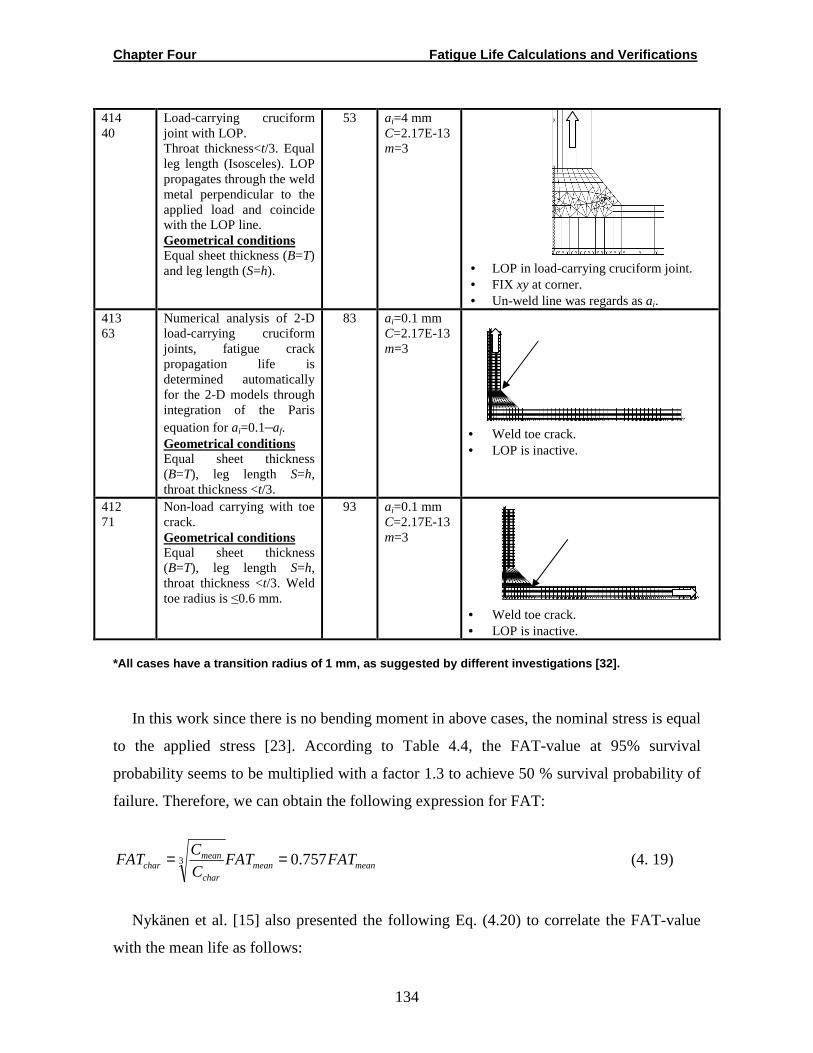
Chapter Four Fatigue Life Calculations and Verifications
134
414 40
Load-carrying cruciform joint with LOP. Throat thickness<t/3. Equal leg length (Isosceles). LOP propagates through the weld metal perpendicular to the applied load and coincide with the LOP line. Geometrical conditions Equal sheet thickness (B=T) and leg length (S=h).
53 ai=4 mm C=2.17E-13 m=3
• LOP in load-carrying cruciform joint. • FIX xy at corner. • Un-weld line was regards as ai.
413 63
Numerical analysis of 2-D load-carrying cruciform joints, fatigue crack propagation life is determined automatically for the 2-D models through integration of the Paris equation for ai=0.1–af. Geometrical conditions Equal sheet thickness (B=T), leg length S=h, throat thickness <t/3.
83 ai=0.1 mm C=2.17E-13 m=3
• Weld toe crack. • LOP is inactive.
412 71
Non-load carrying with toe crack. Geometrical conditions Equal sheet thickness (B=T), leg length S=h, throat thickness <t/3. Weld toe radius is ≤0.6 mm.
93 ai=0.1 mm C=2.17E-13 m=3
• Weld toe crack. • LOP is inactive.
*All cases have a transition radius of 1 mm, as suggested by different investigations [32].
In this work since there is no bending moment in above cases, the nominal stress is equal
to the applied stress [23]. According to Table 4.4, the FAT-value at 95% survival
probability seems to be multiplied with a factor 1.3 to achieve 50 % survival probability of
failure. Therefore, we can obtain the following expression for FAT:
meanmeanchar
meanchar FATFAT
C
CFAT 757.03 == (4. 19)
Nykänen et al. [15] also presented the following Eq. (4.20) to correlate the FAT-value
with the mean life as follows:
Chapter Four Fatigue Life Calculations and Verifications
135
meanmeanchar
meanchar FATFAT
C
CFAT 8275.03 == (4.20)
4.10. Effect of Residual Stresses
The residual stress has an important role on fatigue crack growth. Some researches have
investigated the influence of welding residual stresses for crack growth analyses. The
residual stresses might greatly influence the life or the geometry of the crack after growth.
The influence has been investigated for through-wall cracks by some investigators, but
there were only a few investigations for surface cracks, and the influence has not been
revealed [99]. Usually, the effect of residual stresses and thickness are ignorable for sheet
thickness less than 20 mm [20, 84].
The suggestion for the next Chapter Five is to investigate the influence of residual
stresses on fatigue life curves for a surface crack analytically using the weight function
which assumed a nonlinear stress field present through the thickness.
4.11. Effect of Sheet Thickness
FAT takes an increasing thickness of more than 25 mm into account with a reduction
factor f(t). As a complement to the testing, fracture mechanics calculations are made in an
attempt to evaluate the effect of the stress concentration thickness dependence.
The stress concentration is defined as a local rise of stresses due to a geometrical change
cross section reduction or discontinuity. A more or less abrupt change in geometry is often
referred to as a notch.
Typical stress concentrations due to notches are shown in Figure 4.21. In this case, no
reduction of the cross section is presented, but overfill of the weld metal will act as a stress
riser. The stress will rise at the transition between the base plate and weld metal. This area
is often referred to as the weld toe. This is the potential crack initiation position [1].
The local geometry can be characterized by its flank angle θ and radius ρ. According to
Figure 4.21, the stress concentration factor is defined as [1]:

Chapter Four Fatigue Life Calculations and Verifications
136
ntK
σσ1= (4.21)
where, σn is nominal stress which can be defined in the section away from the notch or
the nominal stress in the notch section, σ1 the local notch stress.
Figure 4.21: Stress concentrations at notches of butt joint [1]
The geometry of the item is important and is one of the issues that must be addressed at
the design stage to achieve improved fatigue durability. The main issue is to reduce the
stress concentration factor Kt in areas susceptible to fatigue [1].
To compile the geometric part of the thickness effects and validate the testing, a fracture
mechanics analysis is carried out. Therefore, the plate thickness correction factor is not
required in the case of assessment based on fracture mechanics procedures or effective
notch stress [3, 34].
It is regarded that this neglecting of thickness’ effect in fracture mechanics method
return to the stress concentration phenomena. As the sheet thickness increases the stress
concentration (Kt) will increase in local points where the crack has assumed and expected
to initiate and propagate according to mechanisms of fracture mechanics method of
materials.
Chapter Four Fatigue Life Calculations and Verifications
137
From a fracture mechanics point of view the stress gradient effect can be understood
because a crack at the surface of a thick plate will grow for a greater distance at a higher
stress level as compared to a crack of the same length in a thin plate for the same surface
stress. Thus, the thinner specimen will have a longer fatigue life [15]. Therefore, as the
sheet thickness increases, the fatigue life strength (FAT) decreases without needs to the
reduction factor as based on fracture mechanics point of view.
To verify this situation, one example of transverse butt weld joint was studied with FE
simulation. Figure 4.22 shows the effect of sheet thickness on the stress distribution of
transverse butt weld joints. The maximum stress at the weld toe decreases when the
thickness increases from 10 mm to 40 mm at constant weld bead height and weld bead
width equal to 2 mm and 10 mm, respectively.
Several iterations of the same model were analysed to select an appropriate mesh density
and subdividing segments. The problems of missing elements and meshes commonly occur
when using a fine mesh density, or inappropriate mesh ratio especially at the corners and
edges. Anther problem is the crack increment when using a fine mesh, i.e., the crack is not
able to reach its final length (one-half of the plate thickness). It is recommended to use
larger increment for such problem in case it does not affect the SIF solution.
Moreover, the problem of memory spaces to solve certain cases will appear for a big
geometry with large number of meshes, high meshes density at the corners, and multi
subdivided areas.
Figure 4.23 and 4.24 show the effect of thickness on the local stress and stress
concentration at the weld toe.
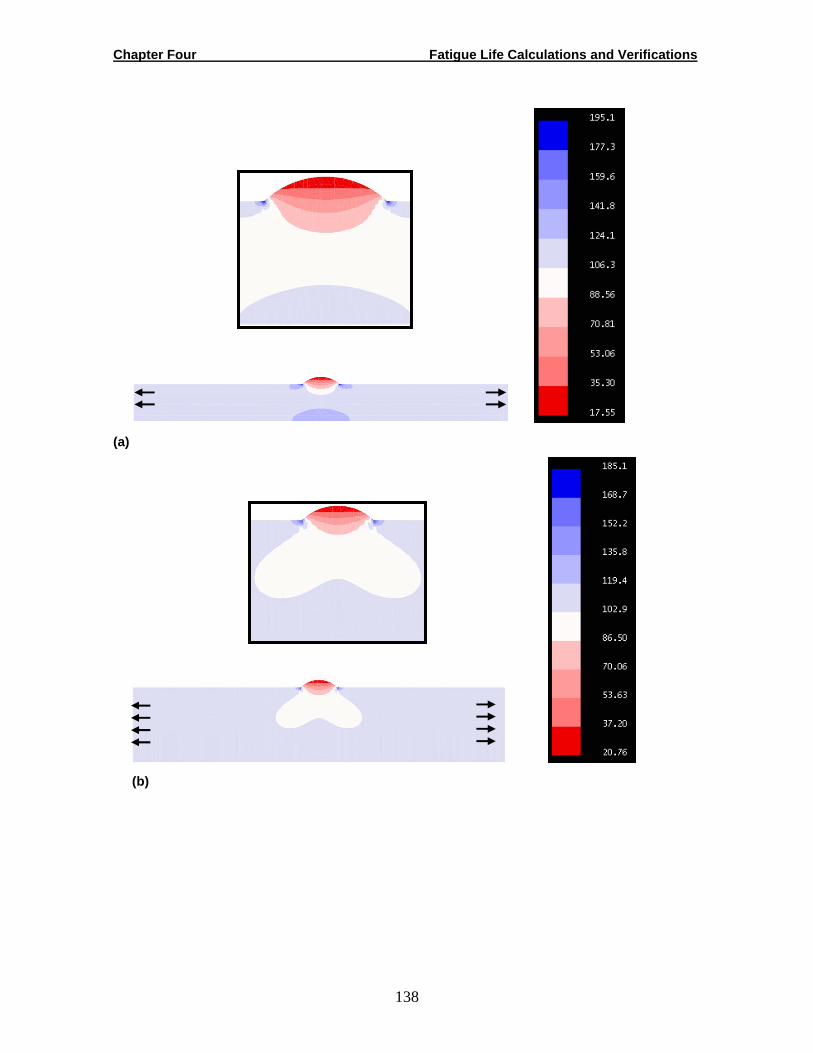
Chapter Four Fatigue Life Calculations and Verifications
138
(a)
(b)
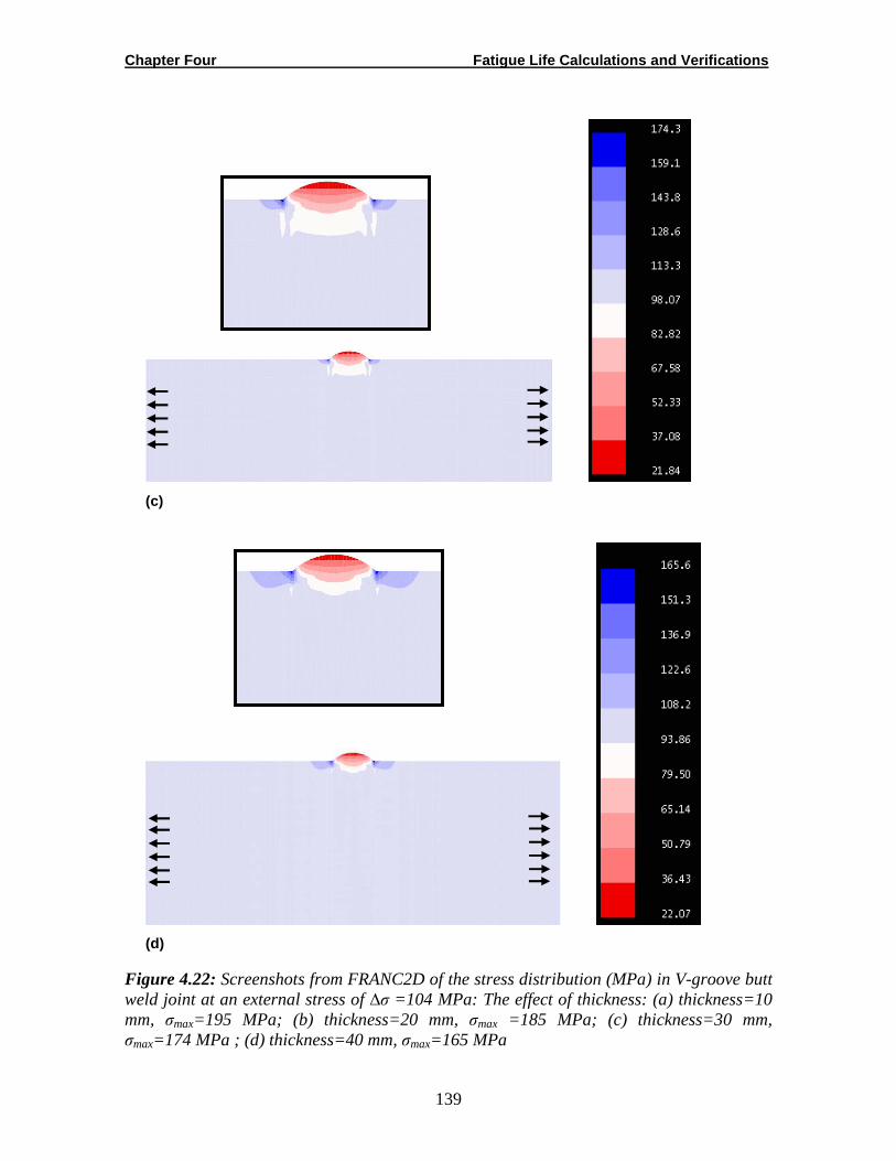
Chapter Four Fatigue Life Calculations and Verifications
139
(c)
(d)
Figure 4.22: Screenshots from FRANC2D of the stress distribution (MPa) in V-groove butt weld joint at an external stress of ∆σ =104 MPa: The effect of thickness: (a) thickness=10 mm, σmax=195 MPa; (b) thickness=20 mm, σmax =185 MPa; (c) thickness=30 mm, σmax=174 MPa ; (d) thickness=40 mm, σmax=165 MPa
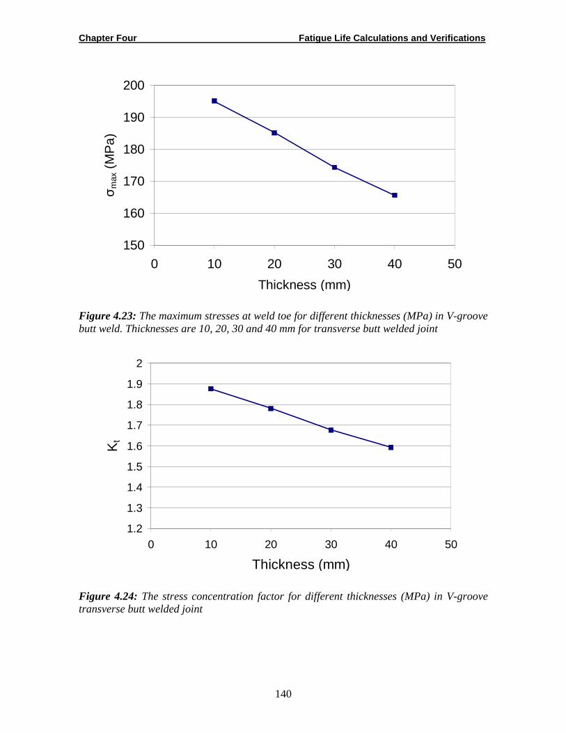
Chapter Four Fatigue Life Calculations and Verifications
140
150
160
170
180
190
200
0 10 20 30 40 50
Thickness (mm)
σm
ax (
MP
a)
Figure 4.23: The maximum stresses at weld toe for different thicknesses (MPa) in V-groove butt weld. Thicknesses are 10, 20, 30 and 40 mm for transverse butt welded joint
1.2
1.3
1.4
1.5
1.6
1.7
1.8
1.9
2
0 10 20 30 40 50
Thickness (mm)
Kt
Figure 4.24: The stress concentration factor for different thicknesses (MPa) in V-groove transverse butt welded joint
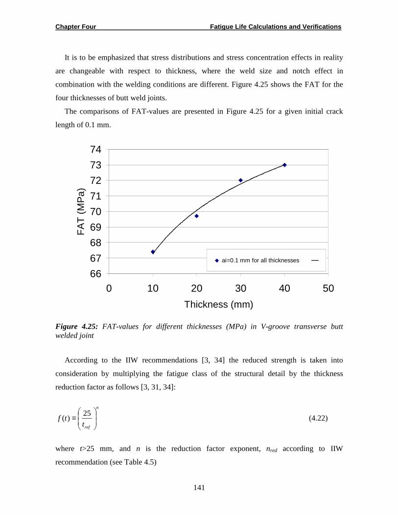
Chapter Four Fatigue Life Calculations and Verifications
141
It is to be emphasized that stress distributions and stress concentration effects in reality
are changeable with respect to thickness, where the weld size and notch effect in
combination with the welding conditions are different. Figure 4.25 shows the FAT for the
four thicknesses of butt weld joints.
The comparisons of FAT-values are presented in Figure 4.25 for a given initial crack
length of 0.1 mm.
66
67
68
69
70
71
72
73
74
0 10 20 30 40 50
Thickness (mm)
FA
T (
MP
a)
ai=0.1 mm for all thicknesses
Figure 4.25: FAT-values for different thicknesses (MPa) in V-groove transverse butt welded joint
According to the IIW recommendations [3, 34] the reduced strength is taken into
consideration by multiplying the fatigue class of the structural detail by the thickness
reduction factor as follows [3, 31, 34]:
n
refttf
= 25
)( (4.22)
where t>25 mm, and n is the reduction factor exponent, nred according to IIW
recommendation (see Table 4.5)
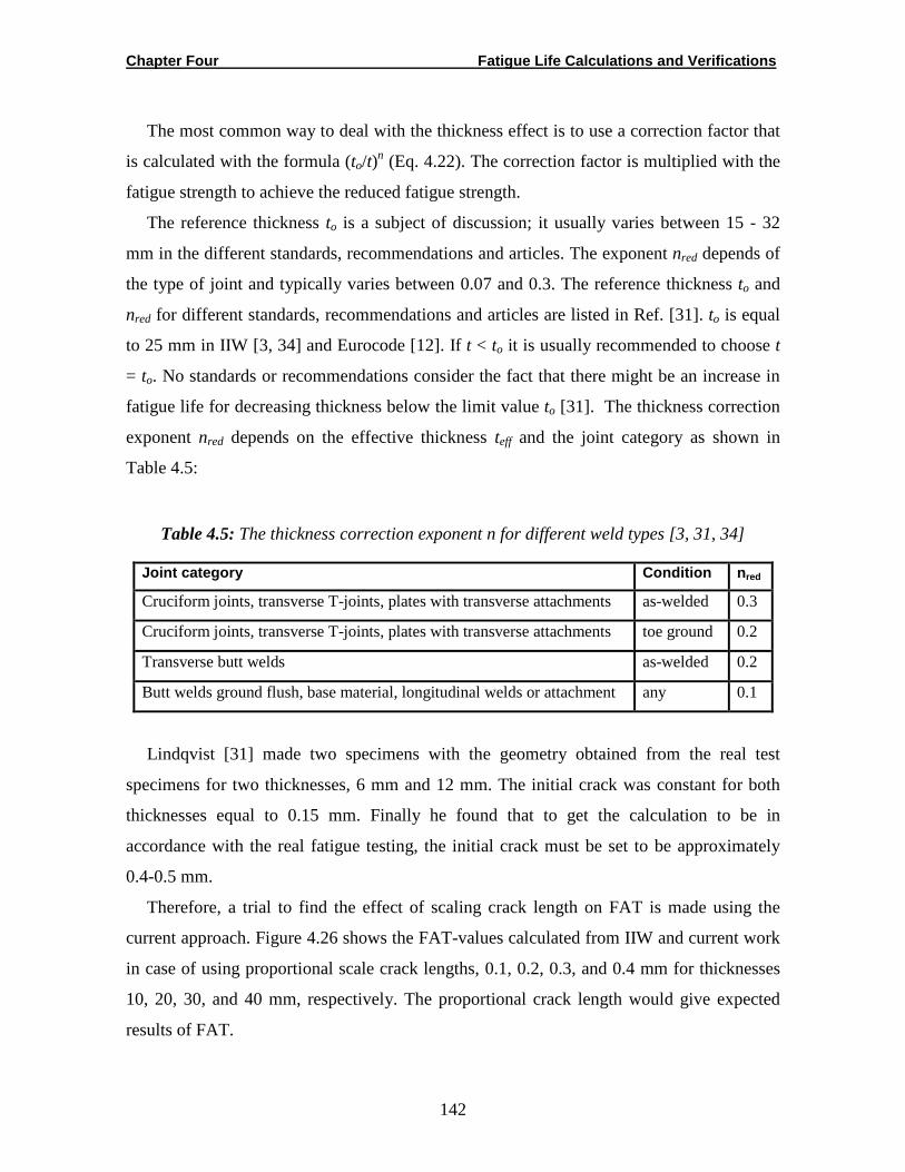
Chapter Four Fatigue Life Calculations and Verifications
142
The most common way to deal with the thickness effect is to use a correction factor that
is calculated with the formula (to/t)n (Eq. 4.22). The correction factor is multiplied with the
fatigue strength to achieve the reduced fatigue strength.
The reference thickness to is a subject of discussion; it usually varies between 15 - 32
mm in the different standards, recommendations and articles. The exponent nred depends of
the type of joint and typically varies between 0.07 and 0.3. The reference thickness to and
nred for different standards, recommendations and articles are listed in Ref. [31]. to is equal
to 25 mm in IIW [3, 34] and Eurocode [12]. If t < to it is usually recommended to choose t
= to. No standards or recommendations consider the fact that there might be an increase in
fatigue life for decreasing thickness below the limit value to [31]. The thickness correction
exponent nred depends on the effective thickness teff and the joint category as shown in
Table 4.5:
Table 4.5: The thickness correction exponent n for different weld types [3, 31, 34]
Joint category Condition nred
Cruciform joints, transverse T-joints, plates with transverse attachments as-welded 0.3
Cruciform joints, transverse T-joints, plates with transverse attachments toe ground 0.2
Transverse butt welds as-welded 0.2
Butt welds ground flush, base material, longitudinal welds or attachment any 0.1
Lindqvist [31] made two specimens with the geometry obtained from the real test
specimens for two thicknesses, 6 mm and 12 mm. The initial crack was constant for both
thicknesses equal to 0.15 mm. Finally he found that to get the calculation to be in
accordance with the real fatigue testing, the initial crack must be set to be approximately
0.4-0.5 mm.
Therefore, a trial to find the effect of scaling crack length on FAT is made using the
current approach. Figure 4.26 shows the FAT-values calculated from IIW and current work
in case of using proportional scale crack lengths, 0.1, 0.2, 0.3, and 0.4 mm for thicknesses
10, 20, 30, and 40 mm, respectively. The proportional crack length would give expected
results of FAT.
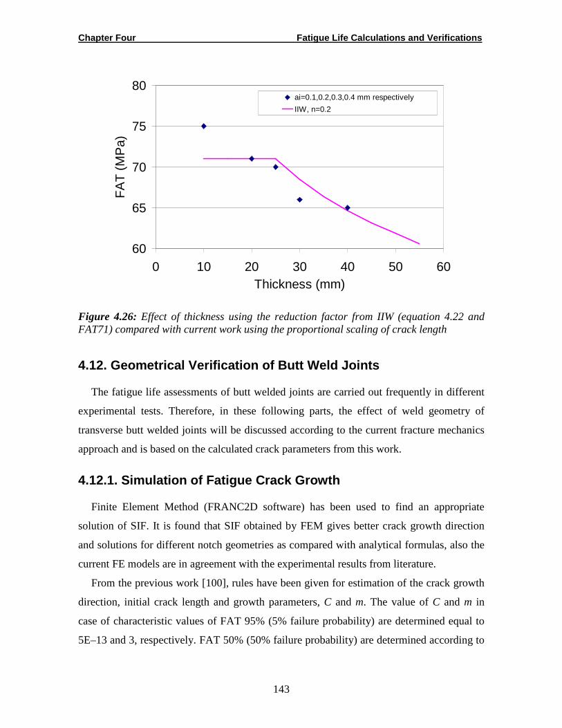
Chapter Four Fatigue Life Calculations and Verifications
143
60
65
70
75
80
0 10 20 30 40 50 60Thickness (mm)
FA
T (
MP
a)
ai=0.1,0.2,0.3,0.4 mm respectively
IIW, n=0.2
Figure 4.26: Effect of thickness using the reduction factor from IIW (equation 4.22 and FAT71) compared with current work using the proportional scaling of crack length
4.12. Geometrical Verification of Butt Weld Joints
The fatigue life assessments of butt welded joints are carried out frequently in different
experimental tests. Therefore, in these following parts, the effect of weld geometry of
transverse butt welded joints will be discussed according to the current fracture mechanics
approach and is based on the calculated crack parameters from this work.
4.12.1. Simulation of Fatigue Crack Growth
Finite Element Method (FRANC2D software) has been used to find an appropriate
solution of SIF. It is found that SIF obtained by FEM gives better crack growth direction
and solutions for different notch geometries as compared with analytical formulas, also the
current FE models are in agreement with the experimental results from literature.
From the previous work [100], rules have been given for estimation of the crack growth
direction, initial crack length and growth parameters, C and m. The value of C and m in
case of characteristic values of FAT 95% (5% failure probability) are determined equal to
5E–13 and 3, respectively. FAT 50% (50% failure probability) are determined according to
Chapter Four Fatigue Life Calculations and Verifications
144
C50% and m equal to 2.17E–13 and 3, respectively. The FEA is used to simulate fatigue
crack growth. As a fatigue crack propagates, the re-meshing process will be carried out
automatically using FRANC2D program.
Figure 4.27 presents the simulated and real experimentally tested specimens, where W is
the reinforcement width (weld bead width) and H the reinforcement height (weld bead
height). Fatigue crack growth is simulated under the opening mode-I which is usually
assumed in fracture mechanics.
(a) (b)
Figure 4.27: Transverse butt weld joints: (a) experimental crack [101]; (b) crack growth simulation by FRANC2D
It has been shown that fatigue crack growth behaviors of welded joints are highly
dependent not only on the materials and load conditions, but also on weld geometry such as
weld toe angle, weld toe radius, plate thickness and width of reinforcements (the weld
bead) [28]. Nguyen et al. [50] used LEFM to present the effects of tip radius of undercut at
weld toe, weld toe radius, flank angle, plate thickness and edge preparation angle on the
fatigue crack propagation life. In addition, the current work highlights on the weld bead
height, weld bead width and on sheet thickness effects which are regarded the main factors
which connect the other remaining parameters. Cracks occur at the weld toe where high
residual tensile stresses are introduced by the welding processes due to the expansion and
the shrinkage of weldment during heating and cooling, misalignment and microstructural
variation in weldment and HAZ, see Figure 4.27.
Chapter Four Fatigue Life Calculations and Verifications
145
4.12.2. Failure Mode
Due to symmetry, the half models can be used to determine the fatigue propagation life
under cyclic tensile loading, as described in Chapter Three. The majority of crack initiation
is at geometrical discontinuities such as weld toe and weld defects. The maximum depths at
the fatigue crack initiation points are found to be less than 0.016 in., or 0.4 mm. While the
maximum distance from the weld surface to the embedded defects is about 0.08 in., or 2
mm [22, 102]. Therefore, it can be supposed that the initial crack length has a range
between 0.4-2 mm. The uncertainly of initial crack lengths is incredible and leads to serious
results; therefore, for all the models, an initial crack depth of weld toe crack of 0.1 mm is
used as predicted before.
The FEM simulation by FRANC2D shows that the maximum stress intensities develop
when the plane of the crack is normal to the direction of the primary tensile stress (opening
mode). However, as the plane of the crack tilts further away from the mode-I tensile
loading, the structural member, in the form of a plate or a similar configuration, will lose its
ability to support the external load.
4.12.3. Weld Metallurgy and Defects
It has been generally recognized that welded structures contain defects, either built in
during fabrication or initiated early under service conditions. When the structures are
subjected to variable cyclic stress, fatigue cracks are initiated from these defects and
propagated from a sub-critical to a critical size. These cracks are usually initiated at the
weld toe. Therefore, welds are prime target in most failures. Subtle peculiarities lie at the
root of many weld designs. These are related to the heat-affected zone (HAZ), weld proper
and the fusion line. The fusion line seldom propagates fracture unless it becomes very
brittle. More description of several principal type of cracking that can occur during or after
welding can be found elsewhere [103].
Impurities consisting of a small amount of sulfur and phosphorus are critical to hot
cracking of steel which mechanism of cracking it appears at high temperature before the
metal develops sufficient strength, see Figure 4.28. Cold cracking occurs after hard
products such as bainite and martensites are formed [103].

Chapter Four Fatigue Life Calculations and Verifications
146
The main cause can be treated to inherent metallurgical sensitivities and un-proper
weldment. Figure 4.28 shows some of the traditional weld defects.
For welded joints, the presence of weld imperfections such as slag inclusions at weld
toes, undercut, residual stresses, lack of penetration LOP etc., effectively will reduce the
initiation phase. All welded joints contain small slag inclusions at the weld toe, which acts
as pre-existing cracks and stress-raisers. Fatigue crack propagation commences from these
inclusions very early in the life [8]. By contrast to fracture mechanics, cracks are assumed
in those regions according to Figure 4.28.
Figure 4.28: Butt weld defects; toe crack, undercut condition and hot cracking, after [103]
Nevertheless, other defects can be found due to non proper weld technique and
fabrication faults. Therefore, most researchers and engineers used to assume that there are
crack-like defects in welds [39]. Then the total fatigue life of welded joints NT is the stress
cycles devoted to the crack growth from these defects to final failure i.e., NT=NP.
Lindqvist [31] showed a 12 mm specimen’s fracture surface after it was fatigue tested
and afterwards broken up. Probably there were several small cracks along the weld toe.
When the cracks grew in the direction normal to the applied load they united into one large
semi-elliptical crack in direction normal to applied load. These behaviours are quite similar
for most joints having toe cracks.
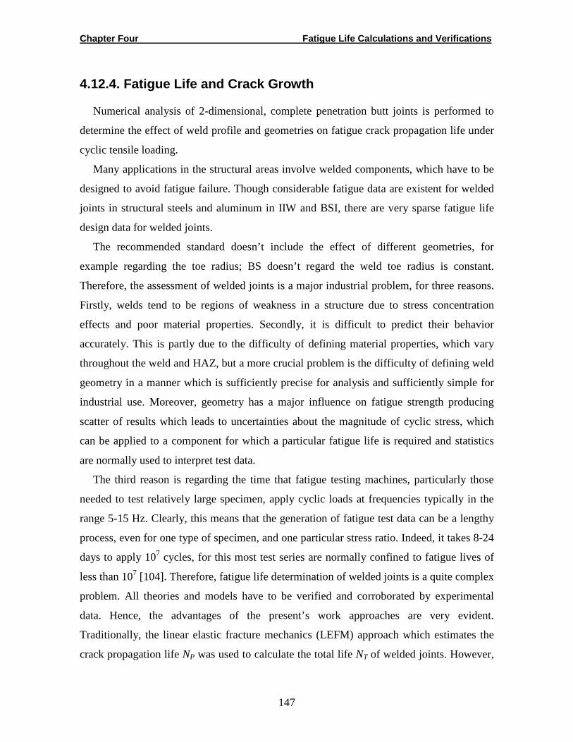
Chapter Four Fatigue Life Calculations and Verifications
147
4.12.4. Fatigue Life and Crack Growth
Numerical analysis of 2-dimensional, complete penetration butt joints is performed to
determine the effect of weld profile and geometries on fatigue crack propagation life under
cyclic tensile loading.
Many applications in the structural areas involve welded components, which have to be
designed to avoid fatigue failure. Though considerable fatigue data are existent for welded
joints in structural steels and aluminum in IIW and BSI, there are very sparse fatigue life
design data for welded joints.
The recommended standard doesn’t include the effect of different geometries, for
example regarding the toe radius; BS doesn’t regard the weld toe radius is constant.
Therefore, the assessment of welded joints is a major industrial problem, for three reasons.
Firstly, welds tend to be regions of weakness in a structure due to stress concentration
effects and poor material properties. Secondly, it is difficult to predict their behavior
accurately. This is partly due to the difficulty of defining material properties, which vary
throughout the weld and HAZ, but a more crucial problem is the difficulty of defining weld
geometry in a manner which is sufficiently precise for analysis and sufficiently simple for
industrial use. Moreover, geometry has a major influence on fatigue strength producing
scatter of results which leads to uncertainties about the magnitude of cyclic stress, which
can be applied to a component for which a particular fatigue life is required and statistics
are normally used to interpret test data.
The third reason is regarding the time that fatigue testing machines, particularly those
needed to test relatively large specimen, apply cyclic loads at frequencies typically in the
range 5-15 Hz. Clearly, this means that the generation of fatigue test data can be a lengthy
process, even for one type of specimen, and one particular stress ratio. Indeed, it takes 8-24
days to apply 107 cycles, for this most test series are normally confined to fatigue lives of
less than 107 [104]. Therefore, fatigue life determination of welded joints is a quite complex
problem. All theories and models have to be verified and corroborated by experimental
data. Hence, the advantages of the present’s work approaches are very evident.
Traditionally, the linear elastic fracture mechanics (LEFM) approach which estimates the
crack propagation life NP was used to calculate the total life NT of welded joints. However,
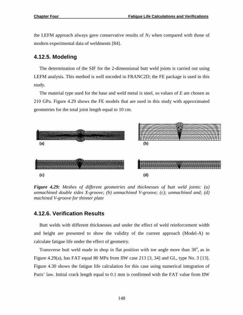
Chapter Four Fatigue Life Calculations and Verifications
148
the LEFM approach always gave conservative results of NT when compared with those of
modern experimental data of weldments [84].
4.12.5. Modeling
The determination of the SIF for the 2-dimensional butt weld joints is carried out using
LEFM analysis. This method is well encoded in FRANC2D; the FE package is used in this
study.
The material type used for the base and weld metal is steel, so values of E are chosen as
210 GPa. Figure 4.29 shows the FE models that are used in this study with approximated
geometries for the total joint length equal to 10 cm.
(a) (b)
(c) (d)
Figure 4.29: Meshes of different geometries and thicknesses of butt weld joints: (a) unmachined double sides X-groove; (b) unmachined V-groove; (c); unmachined and; (d) machined V-groove for thinner plate
4.12.6. Verification Results
Butt welds with different thicknesses and under the effect of weld reinforcement width
and height are presented to show the validity of the current approach (Model-A) to
calculate fatigue life under the effect of geometry.
Transverse butt weld made in shop in flat position with toe angle more than 30o, as in
Figure 4.29(a), has FAT equal 80 MPa from IIW case 213 [3, 34] and GL, type No. 3 [13].
Figure 4.30 shows the fatigue life calculation for this case using numerical integration of
Paris’ law. Initial crack length equal to 0.1 mm is confirmed with the FAT value from IIW
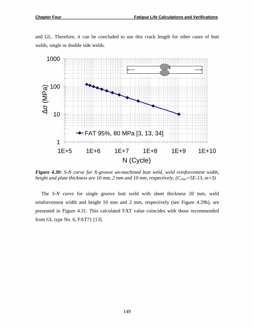
Chapter Four Fatigue Life Calculations and Verifications
149
and GL. Therefore, it can be concluded to use this crack length for other cases of butt
welds, single or double side welds.
1
10
100
1000
1E+5 1E+6 1E+7 1E+8 1E+9 1E+10
N (Cycle)
∆σ
(M
Pa)
FAT 95%, 80 MPa [3, 13, 34]
Figure 4.30: S-N curve for X-groove un-machined butt weld, weld reinforcement width, height and plate thickness are 10 mm, 2 mm and 10 mm, respectively, (Cchar=5E-13, m=3)
The S-N curve for single groove butt weld with sheet thickness 20 mm, weld
reinforcement width and height 10 mm and 2 mm, respectively (see Figure 4.29b), are
presented in Figure 4.31. This calculated FAT value coincides with those recommended
from GL type No. 6, FAT71 [13].
Chapter Four Fatigue Life Calculations and Verifications
150
1
10
100
1000
1E+5 1E+6 1E+7 1E+8 1E+9N (Cycle)
∆σ
(M
Pa)
FAT 95%, un-machined, FAT71, model-A
FAT 95%, 71 MPa [13]
Figure 4.31: S-N curve for V-groove un-machined butt weld, weld reinforcement width, height and plate thickness are 10 mm, 2 mm and 20 mm, respectively, (Cchar=5E-13, m=3)
The stress concentration is increased as a local stress is raised due to the geometrical
change and the weld overfilling.
Overfill of the weld metal will act as a stress riser. This stress rise will of course be very
harmful with respect to fatigue damage. Therefore, and due to the effect of stress
concentration, the fatigue strength decreases with the presence of weld reinforcement.
Hence, the complete removal of the weld bead reinforcement (see Figure 4.29d) is reported
to give improved fatigue performance in condition of free surface from crack-like scratch
after machining. The machining processes for fillet weld is highly effecting on FAT and
fatigue behavior of joints. In this work, the flash grinding increases the calculated FAT to
94 MPa while it was 71 MPa as reported in Ref. [13] in case with weld reinforcement due
to reduction of stress concentration at weld toe, see Figure 4.32. An increase in endurance
limit is also observed in the joint area of flash butt welded joints after the weld flash has
been removed [105].
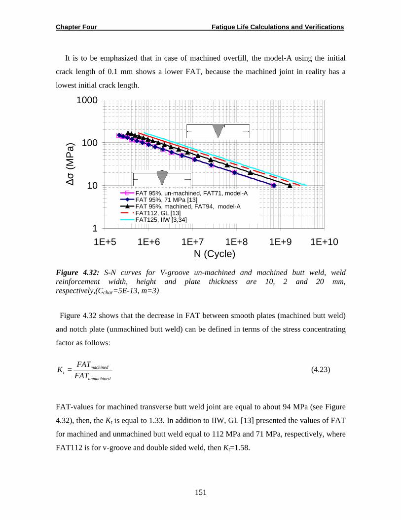
Chapter Four Fatigue Life Calculations and Verifications
151
It is to be emphasized that in case of machined overfill, the model-A using the initial
crack length of 0.1 mm shows a lower FAT, because the machined joint in reality has a
lowest initial crack length.
1
10
100
1000
1E+5 1E+6 1E+7 1E+8 1E+9 1E+10N (Cycle)
∆σ
(M
Pa)
FAT 95%, un-machined, FAT71, model-AFAT 95%, 71 MPa [13]FAT 95%, machined, FAT94, model-AFAT112, GL [13]FAT125, IIW [3,34]
Figure 4.32: S-N curves for V-groove un-machined and machined butt weld, weld reinforcement width, height and plate thickness are 10, 2 and 20 mm, respectively,(Cchar=5E-13, m=3)
Figure 4.32 shows that the decrease in FAT between smooth plates (machined butt weld)
and notch plate (unmachined butt weld) can be defined in terms of the stress concentrating
factor as follows:
unmachined
machinedt FAT
FATK = (4.23)
FAT-values for machined transverse butt weld joint are equal to about 94 MPa (see Figure
4.32), then, the Kt is equal to 1.33. In addition to IIW, GL [13] presented the values of FAT
for machined and unmachined butt weld equal to 112 MPa and 71 MPa, respectively, where
FAT112 is for v-groove and double sided weld, then Kt=1.58.
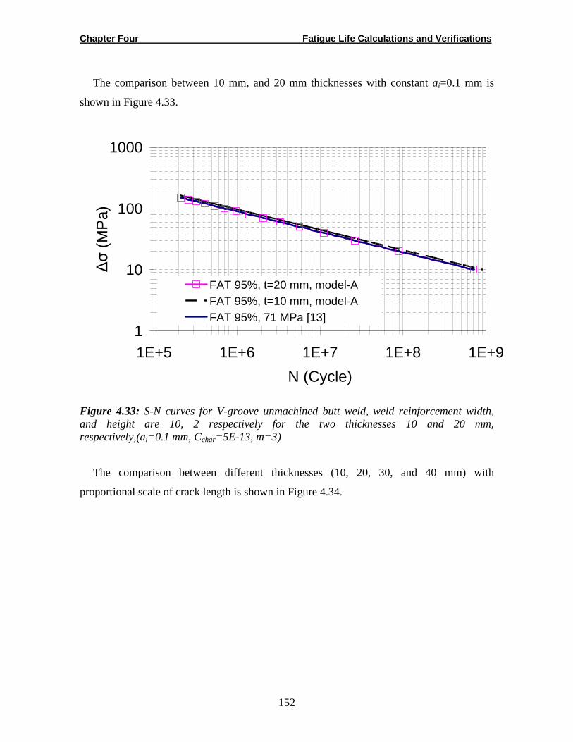
Chapter Four Fatigue Life Calculations and Verifications
152
The comparison between 10 mm, and 20 mm thicknesses with constant ai=0.1 mm is
shown in Figure 4.33.
1
10
100
1000
1E+5 1E+6 1E+7 1E+8 1E+9
N (Cycle)
∆σ
(M
Pa)
FAT 95%, t=20 mm, model-AFAT 95%, t=10 mm, model-AFAT 95%, 71 MPa [13]
Figure 4.33: S-N curves for V-groove unmachined butt weld, weld reinforcement width, and height are 10, 2 respectively for the two thicknesses 10 and 20 mm, respectively,(ai=0.1 mm, Cchar=5E-13, m=3)
The comparison between different thicknesses (10, 20, 30, and 40 mm) with
proportional scale of crack length is shown in Figure 4.34.
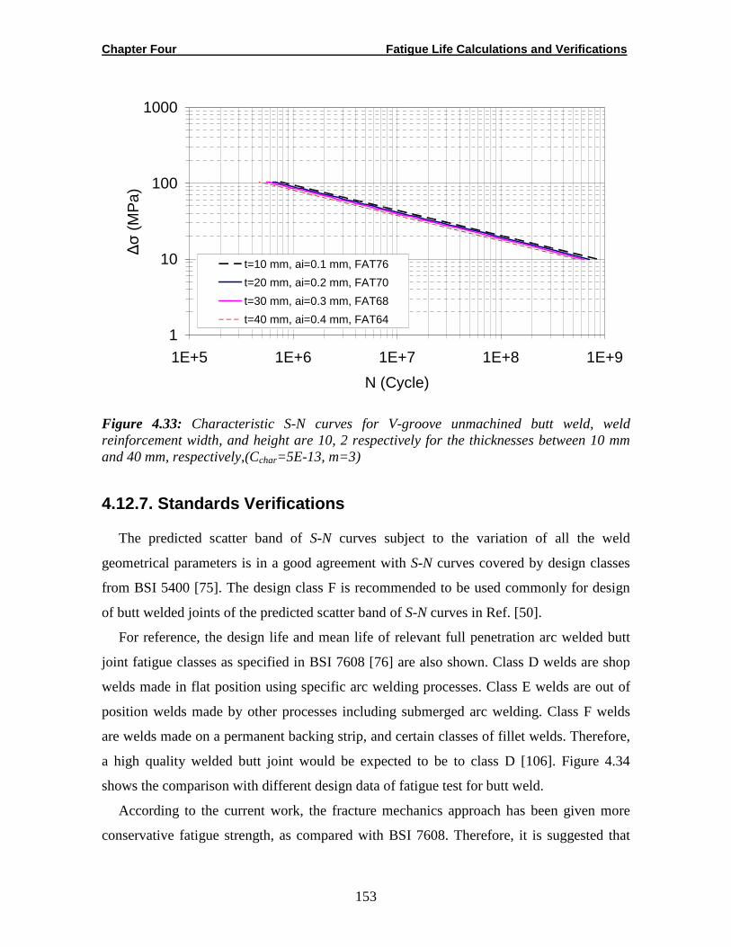
Chapter Four Fatigue Life Calculations and Verifications
153
1
10
100
1000
1E+5 1E+6 1E+7 1E+8 1E+9
N (Cycle)
∆σ
(M
Pa)
t=10 mm, ai=0.1 mm, FAT76
t=20 mm, ai=0.2 mm, FAT70
t=30 mm, ai=0.3 mm, FAT68
t=40 mm, ai=0.4 mm, FAT64
Figure 4.33: Characteristic S-N curves for V-groove unmachined butt weld, weld reinforcement width, and height are 10, 2 respectively for the thicknesses between 10 mm and 40 mm, respectively,(Cchar=5E-13, m=3)
4.12.7. Standards Verifications
The predicted scatter band of S-N curves subject to the variation of all the weld
geometrical parameters is in a good agreement with S-N curves covered by design classes
from BSI 5400 [75]. The design class F is recommended to be used commonly for design
of butt welded joints of the predicted scatter band of S-N curves in Ref. [50].
For reference, the design life and mean life of relevant full penetration arc welded butt
joint fatigue classes as specified in BSI 7608 [76] are also shown. Class D welds are shop
welds made in flat position using specific arc welding processes. Class E welds are out of
position welds made by other processes including submerged arc welding. Class F welds
are welds made on a permanent backing strip, and certain classes of fillet welds. Therefore,
a high quality welded butt joint would be expected to be to class D [106]. Figure 4.34
shows the comparison with different design data of fatigue test for butt weld.
According to the current work, the fracture mechanics approach has been given more
conservative fatigue strength, as compared with BSI 7608. Therefore, it is suggested that
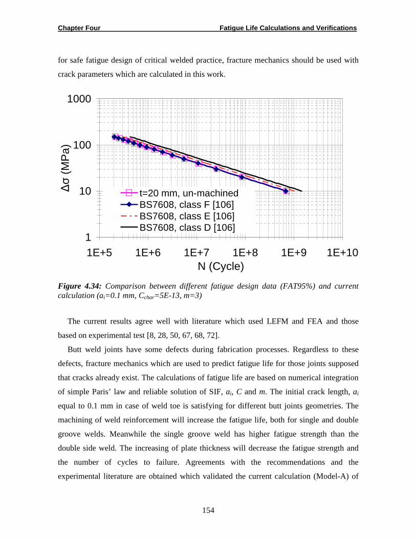
Chapter Four Fatigue Life Calculations and Verifications
154
for safe fatigue design of critical welded practice, fracture mechanics should be used with
crack parameters which are calculated in this work.
1
10
100
1000
1E+5 1E+6 1E+7 1E+8 1E+9 1E+10N (Cycle)
∆σ
(M
Pa)
t=20 mm, un-machinedBS7608, class F [106]BS7608, class E [106]BS7608, class D [106]
Figure 4.34: Comparison between different fatigue design data (FAT95%) and current calculation (ai=0.1 mm, Cchar=5E-13, m=3)
The current results agree well with literature which used LEFM and FEA and those
based on experimental test [8, 28, 50, 67, 68, 72].
Butt weld joints have some defects during fabrication processes. Regardless to these
defects, fracture mechanics which are used to predict fatigue life for those joints supposed
that cracks already exist. The calculations of fatigue life are based on numerical integration
of simple Paris’ law and reliable solution of SIF, ai, C and m. The initial crack length, ai
equal to 0.1 mm in case of weld toe is satisfying for different butt joints geometries. The
machining of weld reinforcement will increase the fatigue life, both for single and double
groove welds. Meanwhile the single groove weld has higher fatigue strength than the
double side weld. The increasing of plate thickness will decrease the fatigue strength and
the number of cycles to failure. Agreements with the recommendations and the
experimental literature are obtained which validated the current calculation (Model-A) of

Chapter Four Fatigue Life Calculations and Verifications
155
initial crack length and convergence study of numerical integration. Hence, that prevents
wasted time to carry out experiments. Therefore, it is suggested that for safe fatigue design
of critical welded practice, fracture mechanics should be used with crack parameters which
were calculated in this work.
4.13. Conclusions
Fracture mechanics is used to find the accurate prediction of fatigue life of welded
joints. It can be used to determine FAT of unknown notch cases of welded connections. In
the literature, different values of cracks length are proposed and presented normally as a
range. Initial cracks take on the responsibility of massive break down. The main purpose
for this study is to determine the crack lengths with the growth parameters. Some
comparisons are carried out with experimental results to detect and identify fatigue life for
more than one type of welded joints and type of cracks. Moreover, the FAT values are
determined, which are a link to specific welded joints.
The entire fatigue process in fillet welded joints is modelled by pure fracture mechanics
approach. The simple version of Paris’ law has been adopted. In this work, the initial crack
depth and growth rate parameters are determined according to backward calculations to
determine FAT. The new values of FAT are calculated according to the predicted existence
of an initial crack. Therefore, the proposed initial crack length is expected to give good
results. An initial crack size equal to 0.1 mm is used for all joints that have weld toe crack,
and this length is typical when arc welding is used and consistent for different welding
processes. The different thicknesses are simulated for transverse butt weld joints and the
effects on stress concentration and fatigue life are presented. It was found that for the
constant initial crack, the FAT will increase as thickness increases due to reduction of stress
concentration factor. However this conclusion is conflicted with the fracture mechanics
point of view, but it is consistent with FE point of view in terms of constant weld geometry
and nominal applied load. The scaling crack length with respect to plate thickness would
give the expected results. The effect of scaling crack length on FAT-curves is also
presented.
The root crack is varied depending on the degree of the penetration. The conventional
crack lengths for joints having LOP or incomplete melting welds metal will be equal to line
Chapter Four Fatigue Life Calculations and Verifications
156
of LOP. These initial crack length values are applicable for all types of joints which have
the same crack type. The cruciform fillet joints with LOP=2 mm show a better FAT value
compared with longer LOP. The FAT value increases as the LOP decreases due to the
increasing crack path to reach final length of failure.
The possibilities for simulating different geometries and calculating the fatigue life for
welded joints that provide the fatigue strength are shown. These possibilities are not yet
listed in previous recommendations. Thus save the time and costs that are needed for
experimental testes. The final crack length has little effect as compared with the effect of
initial crack. Therefore, it is defined to be equal to one-half of the sheet thickness in case of
weld toe when the crack path is perpendicular to the applied load. Some other empirical
equations were used for final crack length in case of LOP. Moreover, final crack length
assumptions are verified from a-N curve, when the number of cycles becomes constant.
Chapter Five Residual Stresses in Welded Joints
157
Chapter Five
RESIDUAL STRESSES IN WELDED JOINTS
5.1. Introduction
The effect of a combination of crack closure and residual stress distributions during the
crack propagation has been investigated rarely.
In general, the modern standards and codes of fatigue design present data corresponding
to the fatigue strength (FAT) of real welded joints. These data include the effect of welding
technology, type of welded component and welding residual stresses. Nevertheless, in
many cases, there is a need to consider the influence of welding residual stresses on the
fatigue life of structural components in greater details.
The residual stresses have an important role on fatigue crack growth. Some studies [5,
65, 95] have investigated the influence of welding residual stresses on crack growth. The
residual stresses might greatly influence the whole fatigue life. The influence of residual
stress has been investigated for through-wall cracks by some researchers, but there were
only a few investigations for surface cracks, and the influence has not been revealed yet
[99].
In this work, the effect of residual stresses during crack growth of an edge crack is
presented. The effect of residual stresses and geometry on the fatigue crack growth life of
welded joints is studied by developing an analytical model using Linear Elastic Fracture
Mechanics (LEFM), superposition method and FE approaches. Various configurations of
residual stresses in welded joints are considered and the corresponding residual SIFs are
calculated by using weight functions methods. The weight function is an analytical method
which is used due to the nonlinear stress fields through the plate thickness.
Fatigue life of welds subjected to residual stress configurations in as welded condition
are calculated by using the NASGRO equation with the total range of SIF (KT) for different
Chapter Five Residual Stresses in Welded Joints
158
applied loading stress ratio (R), and compared with the available experimental data. The
current procedure (Model-C) is verified with results found in the literature.
According to the developed approach from the current study, the effects of residual
stresses and weld joint geometry on the fatigue behaviour of welded joints have been
estimated.
In this chapter the T- and cruciform welded joints with weld toe crack are presented. In
addition, Nykänen et al. [15] presented the fatigue life of transverse butt weld with LOP.
This joint is used in addition to verify and compare the current residual stresses calculation.
5.2. Assumptions in Finite Element Model
The assumptions used in fracture mechanics are:
1. The material is homogeneous, isotropic and linearly elastic.
2. The crack tip is subjected to mode-I where only axial load is applied and mode-II and III
where the biaxial load is applied.
3. The effects of plasticity ahead of the crack tip and in its wake are ignored as assumed by
Alam [8].
In this chapter the effects of plasticity in terms of crack closure will be studied within
the effect of residual stresses.
That "fatigue crack closure" is caused by the effects of local compressive residual
stresses that are naturally developed by the fatigue crack growth mechanisms. On the other
hand, the residual stress field due to welding "already" exists before a fatigue crack grows
through this field (in fact these stresses change as a result of crack growth).
Therefore, the crack experiences a combined effect of a "developing" residual
stress field (due to crack closure) and a "changing" residual stress field (due to welding) in
a quite complex combination. These combinations are considered to be restricted aspects
and complex in several studies. Therefore, the inclusion of the effects of residual stress
distributions, sign and direction are the most interesting challenges. These effects will be
evaluated in this chapter.

Chapter Five Residual Stresses in Welded Joints
159
5.3. Residual Stresses Assessment
Special conservatism is adapted to the fatigue strength to reduce the risk of unexpected
failure due to geometry and residual stress effects.
Due to the high temperature gradients and plastic deformation in the vicinity of the weld
during the welding processes, residual stress fields are invariably set up in the welded
joints.
Usually such stresses are accounted for in safety assessment procedures such as the
British R6 [107] and BS7910 [14]. Since the informations on residual stress distributions,
signs and magnitude in the component are often not directly available, compendia with
recommended upper-bound residual stress profiles for use in analyses are included in
structural integrity assessment procedures for European industry (SINTAP) [69], British
R6, and BSI 7910. These recommended profiles are classified according to the welding
information.
On the other hand residual stress distributions can be measured experimentally by using
different tests such as neutron or x-ray diffraction or they are estimated by using FEM.
Lee et al. [71] determined the residual stress distributions for plate T-butt welds from a
detailed FEA of the welding process and these distributions were compared with those of
the measured data for validation and shown that they have similar profiles. Lee et al. [71]
also determined the linear elastic SIFs using the FEM and examined a new residual stress
distribution which was less restrictive but had lower conservatism when compared with the
analysis results from the measured data and the distributions of R6 and BSI 7910. The
profile is applicable to different geometries of T-plate and tubular T-joints as well as
different steels (Grades S355 and SE702).
Hyeong et al. [61] presented SIFs in welded T-plate and tubular geometries using
measured residual stress distributions, and these are recommended in assessment
procedures. Residual stress distributions were measured along the thickness direction
(crack length up to half of the plate or pipe thicknesses, a/t=0.5) from the weld toe, where
cracks are often found to initiate. The neutron diffraction method was used and stresses
were measured along the thickness direction. A medium strength steel (BS EN 10025
Grade S355) and a high-strength steel (designated SE702, equivalent to the A517 Grade Q
Chapter Five Residual Stresses in Welded Joints
160
steel) have been examined for the T-plate. The former has yield strength of 348 MPa, and
the latter has a yield strength of 700 MPa.
O’Dowd et al. [60] used the neutron diffraction method to determine residual stress
distributions for welded T-plate. These distributions have been measured using neutron
diffraction method which based on measured elastic strains to determine directly the stress
field. They also examined a high-strength steel (700 MPa yield strength) and medium
strength steel (348 MPa yield strength). The welding conditions and procedures were
presented in details in their work. The resultant linear elastic SIF for these measured
residual stress distributions, Kres has been obtained using FEM software package
ABAQUS.
Researches up-to-date depend on FEM to find residual stress distributions and to
calculate SIF including the effect of residual stresses Kres.
Therefore, the sensitive information needed to predict the behaviour of the welded
structures are the residual stress distributions, σ res(x) and residual stress intensity factor
Kres, where x is the vector along the crack path for each crack length increment.
Kres was calculated in the current work by the product of the weight function, m(x,a) and
the crack surface stress distributions, σ res(x). Moreover, in this work, the residual stress
distribution is established by using SINTAP safety assessment procedures assuming the
case of unknown welding conditions. These stress distributions are compared with
experimentally measured data from literature.
In this work, the calculated residual SIFs are compared with the reported data for welded
T-plate from Refs. [60, 61] for medium and high-strength steels. The transverse residual
stress distributions were studied in this work dealing with mode-I fracture, and different
residual stress distribution profile curves are presented using the SINTAP profile equation.
In addition, SIFs have been determined using FEM with the help of fracture mechanics
which are encoded in the FRANC2D program. Kres is calculated by applying point load
along the expected direction line of a toe crack. The latter calculation is less conservative
and it has good agreement with Kres calculated from experimentally measured data is
observed.
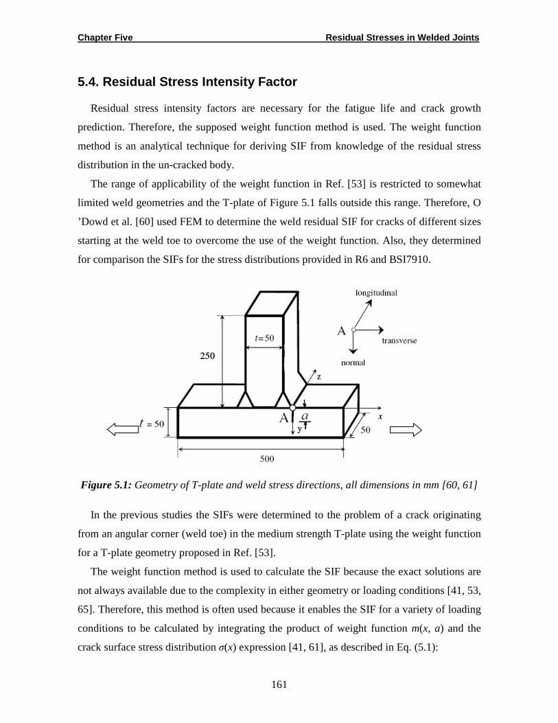
Chapter Five Residual Stresses in Welded Joints
161
5.4. Residual Stress Intensity Factor
Residual stress intensity factors are necessary for the fatigue life and crack growth
prediction. Therefore, the supposed weight function method is used. The weight function
method is an analytical technique for deriving SIF from knowledge of the residual stress
distribution in the un-cracked body.
The range of applicability of the weight function in Ref. [53] is restricted to somewhat
limited weld geometries and the T-plate of Figure 5.1 falls outside this range. Therefore, O
’Dowd et al. [60] used FEM to determine the weld residual SIF for cracks of different sizes
starting at the weld toe to overcome the use of the weight function. Also, they determined
for comparison the SIFs for the stress distributions provided in R6 and BSI7910.
Figure 5.1: Geometry of T-plate and weld stress directions, all dimensions in mm [60, 61]
In the previous studies the SIFs were determined to the problem of a crack originating
from an angular corner (weld toe) in the medium strength T-plate using the weight function
for a T-plate geometry proposed in Ref. [53].
The weight function method is used to calculate the SIF because the exact solutions are
not always available due to the complexity in either geometry or loading conditions [41, 53,
65]. Therefore, this method is often used because it enables the SIF for a variety of loading
conditions to be calculated by integrating the product of weight function m(x, a) and the
crack surface stress distribution σ(x) expression [41, 61], as described in Eq. (5.1):
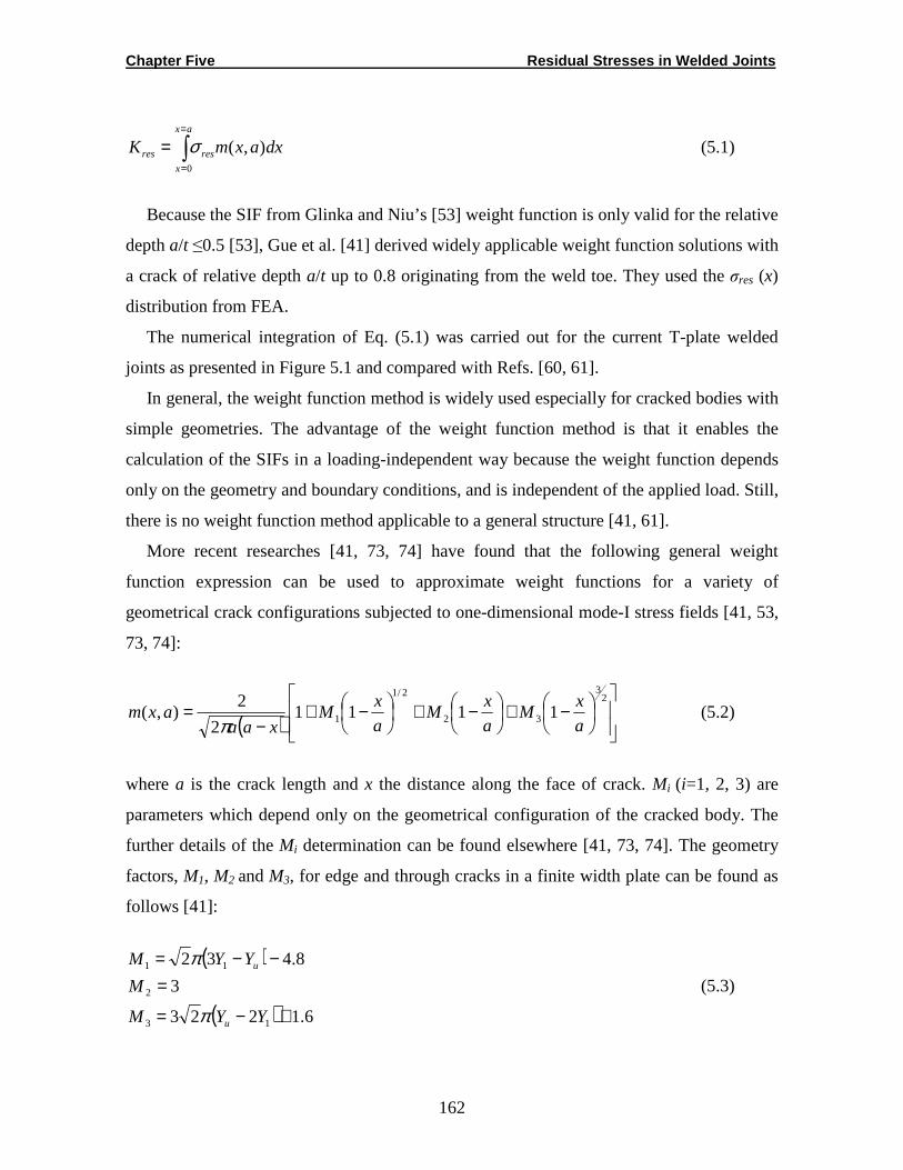
Chapter Five Residual Stresses in Welded Joints
162
dxaxmKax
x
resres ),(0∫=
=
= σ (5.1)
Because the SIF from Glinka and Niu’s [53] weight function is only valid for the relative
depth a/t ≤0.5 [53], Gue et al. [41] derived widely applicable weight function solutions with
a crack of relative depth a/t up to 0.8 originating from the weld toe. They used the σres (x)
distribution from FEA.
The numerical integration of Eq. (5.1) was carried out for the current T-plate welded
joints as presented in Figure 5.1 and compared with Refs. [60, 61].
In general, the weight function method is widely used especially for cracked bodies with
simple geometries. The advantage of the weight function method is that it enables the
calculation of the SIFs in a loading-independent way because the weight function depends
only on the geometry and boundary conditions, and is independent of the applied load. Still,
there is no weight function method applicable to a general structure [41, 61].
More recent researches [41, 73, 74] have found that the following general weight
function expression can be used to approximate weight functions for a variety of
geometrical crack configurations subjected to one-dimensional mode-I stress fields [41, 53,
73, 74]:
( )
−+
−+
−+−
=2
3
32
2/1
1 11112
2),(
a
xM
a
xM
a
xM
xaaaxm
π (5.2)
where a is the crack length and x the distance along the face of crack. Mi (i=1, 2, 3) are
parameters which depend only on the geometrical configuration of the cracked body. The
further details of the Mi determination can be found elsewhere [41, 73, 74]. The geometry
factors, M1, M2 and M3, for edge and through cracks in a finite width plate can be found as
follows [41]:
( )
( ) 6.1223
3
8.432
13
2
11
+−=
=−−=
YYM
M
YYM
u
u
π
π (5.3)
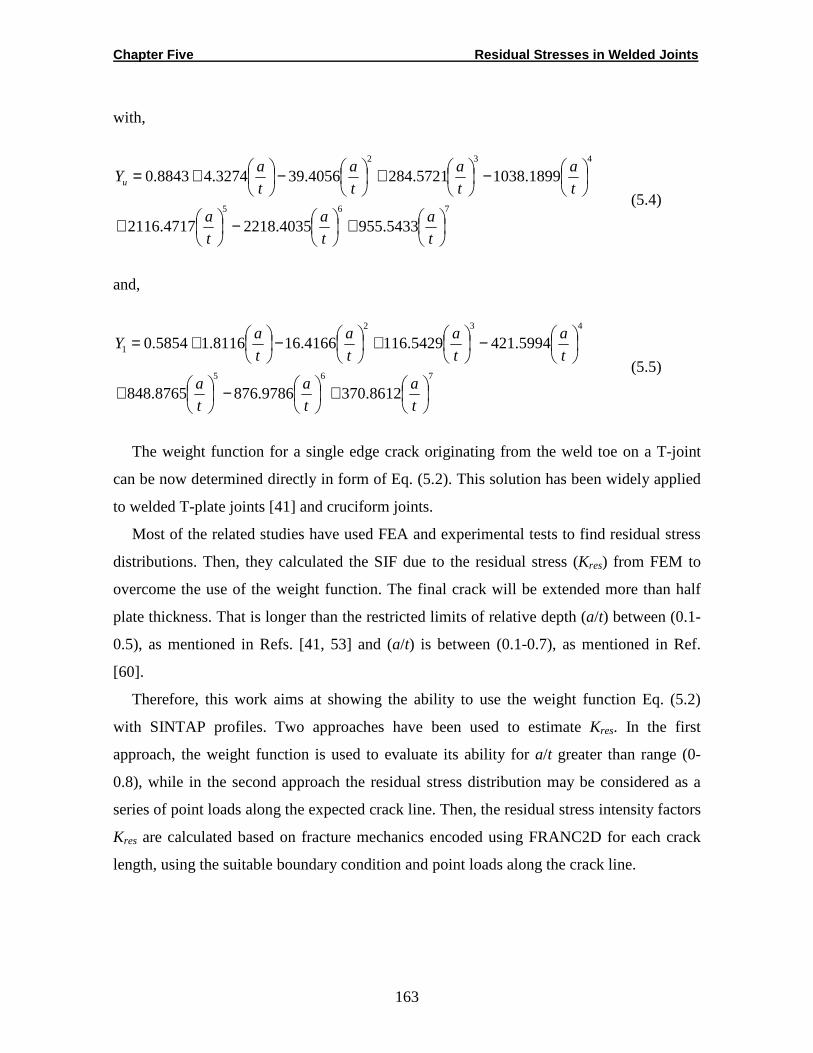
Chapter Five Residual Stresses in Welded Joints
163
with,
765
432
5433.9554035.22184717.2116
1899.10385721.2844056.393274.48843.0
+
−
+
−
+
−
+=
t
a
t
a
t
a
t
a
t
a
t
a
t
aYu
(5.4)
and,
765
432
1
8612.3709786.8768765.848
5994.4215429.1164166.168116.15854.0
+
−
+
−
+
−
+=
t
a
t
a
t
a
t
a
t
a
t
a
t
aY
(5.5)
The weight function for a single edge crack originating from the weld toe on a T-joint
can be now determined directly in form of Eq. (5.2). This solution has been widely applied
to welded T-plate joints [41] and cruciform joints.
Most of the related studies have used FEA and experimental tests to find residual stress
distributions. Then, they calculated the SIF due to the residual stress (Kres) from FEM to
overcome the use of the weight function. The final crack will be extended more than half
plate thickness. That is longer than the restricted limits of relative depth (a/t) between (0.1-
0.5), as mentioned in Refs. [41, 53] and (a/t) is between (0.1-0.7), as mentioned in Ref.
[60].
Therefore, this work aims at showing the ability to use the weight function Eq. (5.2)
with SINTAP profiles. Two approaches have been used to estimate Kres. In the first
approach, the weight function is used to evaluate its ability for a/t greater than range (0-
0.8), while in the second approach the residual stress distribution may be considered as a
series of point loads along the expected crack line. Then, the residual stress intensity factors
Kres are calculated based on fracture mechanics encoded using FRANC2D for each crack
length, using the suitable boundary condition and point loads along the crack line.
Chapter Five Residual Stresses in Welded Joints
164
5.5. Residual Stresses Distribution
Welding processes produce tensile residual stresses in components which have a
significant effect on the integrity of structures. It is therefore important to have a detailed
knowledge about the residual stress distributions in components and their redistribution
after a crack has initiated in the residual stress field.
The existent defect assessment procedures, e.g., BSI 7910, SINTAP and R6, contain
compendia with conservative estimation of the residual stress fields in a number of
structures and materials. Further validation of the recommended residual stress profiles is,
however, required.
A redistribution of stresses in the direction of the thickness gradually occurs as the crack
is propagating. To assess the influence of the residual stresses on the failure of a welded
joint, their distribution must be known. Hence, the failure can be characterized in terms of
LEFM concept.
Although the plate butt welded geometry is the most studied in the literature, there are
also limited informations on residual stress distributions in T-butt joints [69]. T-butt
joints have the same stress distribution which can be used for cruciform joints; therefore,
these joints (T-butt) are considered in this chapter.
The residual stress distributions recommended in the SINTAP compendium of residual
stress profiles have different shapes for different weld geometries and orientations,
including fourth and sixth order polynomials, cosine functions, and piece-wise linear
distributions including bilinear and trapezoidal shapes.
In this work, four types of stress distributions have been examined; namely the BSI 7910
polynomial distribution (SINTAP), an approximate mean stress distribution which refers to
least square linear fits, the proposed upper bound and lower bound distribution which refers
to mean±2STDV, where STDV stands for standard deviation [61]. Figure 5.2 shows the
measurement of the transverse residual stresses of medium-strength and high-strength steel
T-welded plate, which is widely used [60] for a plate thickness of 50 mm. The upper
bound, lower bound and mean least square linear fit stress distributions are shown also in
Figure 5.2.
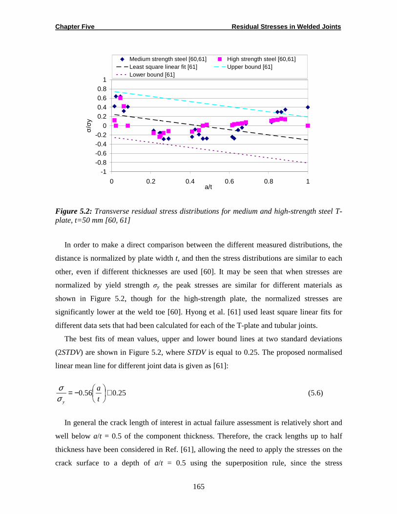
Chapter Five Residual Stresses in Welded Joints
165
-1-0.8-0.6-0.4-0.2
00.20.40.60.8
1
0 0.2 0.4 0.6 0.8 1a/t
σ/σ
y
Medium strength steel [60,61] High strength steel [60,61]Least square linear fit [61] Upper bound [61]Lower bound [61]
Figure 5.2: Transverse residual stress distributions for medium and high-strength steel T-plate, t=50 mm [60, 61]
In order to make a direct comparison between the different measured distributions, the
distance is normalized by plate width t, and then the stress distributions are similar to each
other, even if different thicknesses are used [60]. It may be seen that when stresses are
normalized by yield strength σy the peak stresses are similar for different materials as
shown in Figure 5.2, though for the high-strength plate, the normalized stresses are
significantly lower at the weld toe [60]. Hyong et al. [61] used least square linear fits for
different data sets that had been calculated for each of the T-plate and tubular joints.
The best fits of mean values, upper and lower bound lines at two standard deviations
(2STDV) are shown in Figure 5.2, where STDV is equal to 0.25. The proposed normalised
linear mean line for different joint data is given as [61]:
25.056.0 +
−=t
a
yσσ
(5.6)
In general the crack length of interest in actual failure assessment is relatively short and
well below a/t = 0.5 of the component thickness. Therefore, the crack lengths up to half
thickness have been considered in Ref. [61], allowing the need to apply the stresses on the
crack surface to a depth of a/t = 0.5 using the superposition rule, since the stress

Chapter Five Residual Stresses in Welded Joints
166
distributions over the region of a/t > 0.5 do not influence the SIF values. It is also worthy
noting that the stresses in the region a/t > 0.5 are usually compressive and will have little
effect on SIF values for short cracks [61].
5.6. BSI 7910 Distribution
There are two distributions for residual stress assessments in welded joints, namely R6
and BSI 7910 which are used in SINTAP [69] depending on the available informations
about the welding conditions. If the weld informations are unavailable, then the BSI 7910
polynomial distribution is used. Otherwise, when welding conditions are known or can be
estimated then the stress profiles given are based on the size of the plastic zone which
correlates with the plate thickness, more details are found in Ref. [69]. In the current work,
the BSI 7910 polynomial distribution was used. This distribution is given as:
( ) ( ) ( ) ( )( ) /21.087-/42.485/24.125-/2.32670.97/ 432y tatatata ++=σσ (5.7)
Figure 5.3 shows the SINTAP distribution in value of (σ/σy=97%). The non-conservative
values can be seen as compared with experimental measurements. SINTAP distribution
(σ/σy =50%) has lower values and more satisfy with experimental data (see Eq. 5.8). In the
current work the upper bound stress distributions (SINTAP=0.97, i.e. Eq. 5.7) has been
used.
( ) ( ) ( ) ( )( ) /21.087-/42.485/24.125-/2.32670.5/ 432y tatatata ++=σσ (5.8)
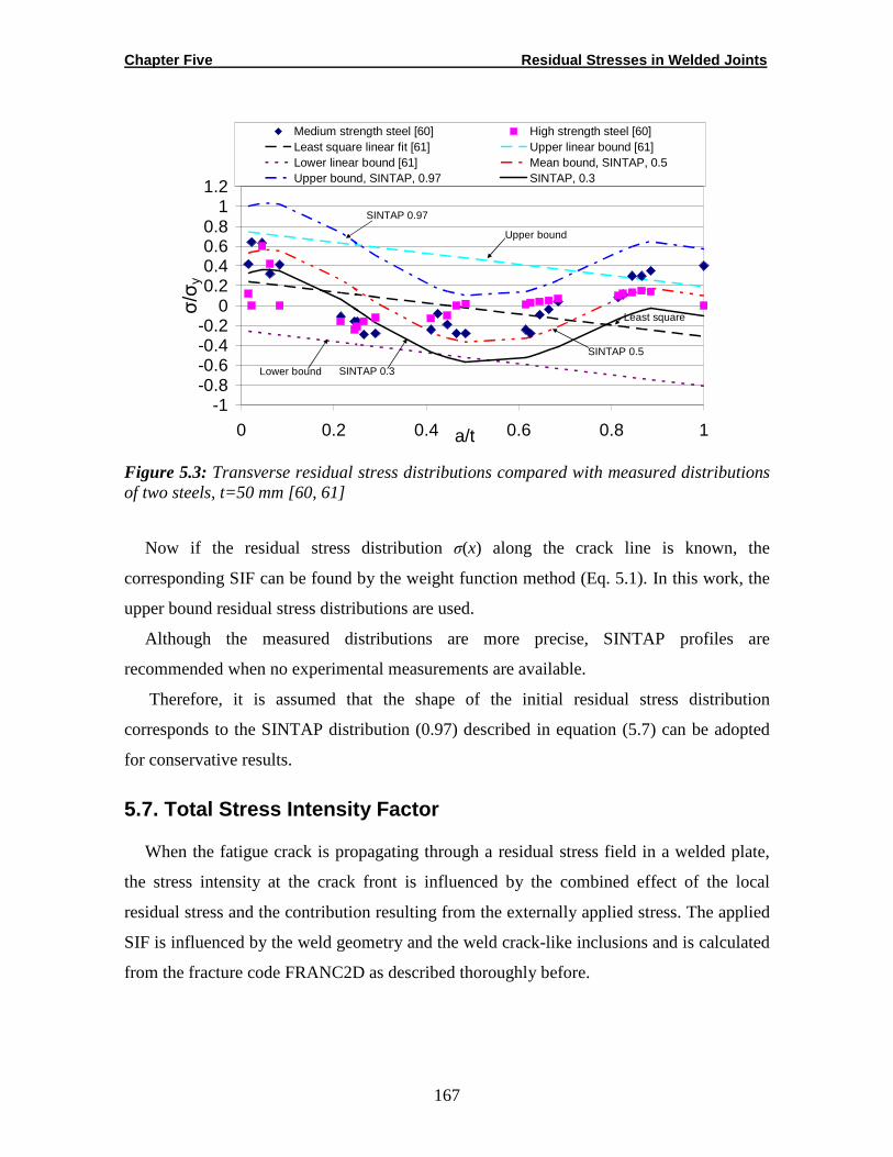
Chapter Five Residual Stresses in Welded Joints
167
-1-0.8-0.6-0.4-0.2
00.20.40.60.8
11.2
0 0.2 0.4 0.6 0.8 1a/t
σ/σ
y
Medium strength steel [60] High strength steel [60]Least square linear fit [61] Upper linear bound [61]Lower linear bound [61] Mean bound, SINTAP, 0.5Upper bound, SINTAP, 0.97 SINTAP, 0.3
Upper bound
SINTAP 0.97
SINTAP 0.5
Lower bound
Least square
SINTAP 0.3
Figure 5.3: Transverse residual stress distributions compared with measured distributions of two steels, t=50 mm [60, 61]
Now if the residual stress distribution σ(x) along the crack line is known, the
corresponding SIF can be found by the weight function method (Eq. 5.1). In this work, the
upper bound residual stress distributions are used.
Although the measured distributions are more precise, SINTAP profiles are
recommended when no experimental measurements are available.
Therefore, it is assumed that the shape of the initial residual stress distribution
corresponds to the SINTAP distribution (0.97) described in equation (5.7) can be adopted
for conservative results.
5.7. Total Stress Intensity Factor
When the fatigue crack is propagating through a residual stress field in a welded plate,
the stress intensity at the crack front is influenced by the combined effect of the local
residual stress and the contribution resulting from the externally applied stress. The applied
SIF is influenced by the weld geometry and the weld crack-like inclusions and is calculated
from the fracture code FRANC2D as described thoroughly before.

Chapter Five Residual Stresses in Welded Joints
168
Therefore, at crack tip, it appears that the actual SIF acting on a stress cycle (KT) does
not have the same magnitude as the applied SIF (Kapp). The differences between the actual
and the effective ∆K vary among different R-ratios.
In order to account the mean stress effect on crack growth rate da/dN, a method to
estimate the effective level of an applied K for a given R-ratio has to be developed. It seems
that the sound approach would be to develop a relationship between effective ∆K and R
based on the concept of crack closure [96]. Different approaches have been developed to be
sensitive with R ratio like NASGRO, Forman, Walker, etc.
The quantities assessment of the influence of a residual stress field on fatigue reliability
can be determined by the principle of superposition based on the total SIF (KT) for the
solution of SIF due to the residual stresses and the solution of the SIF due to external
loading such that:
resappT KKK += (5.9)
The residual stress ratio, Rres in the situation under consideration is defined as:
( )( )resappmax
resmin.appres KK
KKR
++
=,
(5.10)
( )RKK maxeff −=∆ 1 (5.11)
where Kmin,app and Kmax,app are the SIF due to minimum and maximum applied load,
respectively. Kres is the SIF due to the residual stresses which is calculated according to the
current approach. It should be noticed that the range of total stress intensity factor ∆KT does
not change when the residual stresses are superimposed such as [109, 110]:
( ) ( ) ( ) ( )appappminappmax
resappminresmax,appTminTmaxT
KKK
KKKKKKK
∆=−=
+−+=−=∆
,,
, (5.12)
and only the stress ratio, R is affected where Rapp≠Rres.
This indicates that the approach for crack growth in residual stress field should include
the residual stress ratio Rres, in addition to the stress range ∆σ, and SIF range ∆K. This
approach requires the residual stress distribution and the associated stress intensity factor
Chapter Five Residual Stresses in Welded Joints
169
(SIF) which also depends on the fatigue crack length. It has been known that the welding
residual stresses are distributed in a considerably non-uniform manner and are redistributed
during the process of cyclic loading and fatigue crack growth.
The use of superposition has been criticized by some researchers because it considers
only the initial residual stress field that exists in the un-cracked structures, with no
acknowledge of the redistribution of residual stresses that occurs during the propagation of
the fatigue crack. Therefore, Wu [28] mentioned that it is difficult to apply this approach
for effective SIF evaluation because of the difficulty in capturing the actual residual
stresses during crack propagation.
Other researchers have argued that the redistribution of residual stresses is of no
consequence, e.g. LaRue et al. [110] showed that the slotting processes for purpose of
starting a fatigue crack from a hole introduces a redistribution of the residual stresses
although this did not have a considerable effect on the subsequent fatigue life.
Nevertheless to criticizing, superposition based technique is used extensively and it has
been evaluated in the current work.
5.8. Crack Growth Propagation Life
The entire crack growth over the three regions needs to be mathematically approached to
determine the fatigue crack growth like Forman, Walker, and NASGRO equations in terms
of the range of total SIF. The latter is incorporated to calculate Rres using the superposition
method.
5.9. The FNK Equation
The presence of residual stresses influences the crack growth rate da/dN value by
considering the residual stress intensity ratio Rres. The FNK equation is considered the most
suitable for the present study. Here, “FNK” stands for Forman, Newman and de Konig [96].
The equation is used in the most recent release of the crack growth prediction program,
NASGRO. The NASGRO equation is written as:
Chapter Five Residual Stresses in Welded Joints
170
q
c
p
thn
ESA
K
K
K
K
KR
fC
dN
da
−
∆
∆−
∆
−−=
max1
1
1
1 (5.13)
where CESA and n are empirical parameters describing the linear region of the curve (similar
to the Paris’ model), and p and q are empirical constants describing the curvature in fatigue
crack growth rate (FCG) data that occur near threshold (Region-I) and near instability
(Region-III), respectively. The Newman’s effective stress ratio (f), the threshold value of
SIF range for a given R, (∆Kth) and the critical SIF (Kc) are presented in Chapter Four
above. The unit for the fatigue crack growth rate (FCG) da/dN is mm/cycle, and the SIF
range ∆K is MPa (m)1/2.
5.10. Results Verification and Procedures
In this study, a comprehensive program is established to calculate the fatigue life of
welded joints using a language programming. The input equation is SIF from FRANC2D.
This approach includes:
1. Calculations of SIF due to the residual stresses.
2. Incorporations of different residual stress distributions.
3. Calculations of fatigue life and crack growth rate of welded joints, taking into account
the effect of residual stress distributions, applied and residual stress ratio.
According to NASGRO equation, the crack propagation rate for a given Rapp ratio was
predicated by changing the Rres-ratio caused by varying Kres (Model-C). The latter was
calculated as a product of the weight function and the residual stress distributions (Eq. 5.1).
The material data which are necessary for (Eq. 5.13) were obtained from AFGROW
database [97] and Ref. [98], see Table 5.1 for steel S403.
The numerical integration has been carried out with help of FORTRAN language
program to find Kres, and then the fatigue crack growth rate and the fatigue life are
calculated. Two R ratios are incorporated in the program, namely, Rres and Rapp. The former
is calculated from Eq. (5.10) and incorporates the Newman’s effective stress ratio which
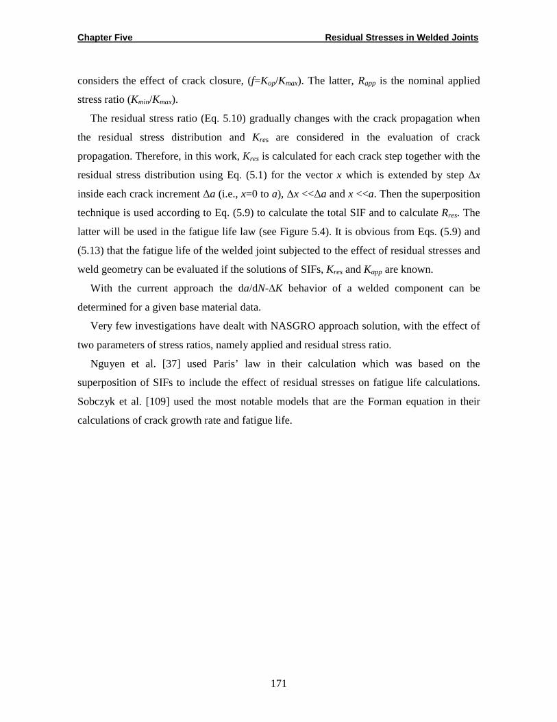
Chapter Five Residual Stresses in Welded Joints
171
considers the effect of crack closure, (f=Kop/Kmax). The latter, Rapp is the nominal applied
stress ratio (Kmin/Kmax).
The residual stress ratio (Eq. 5.10) gradually changes with the crack propagation when
the residual stress distribution and Kres are considered in the evaluation of crack
propagation. Therefore, in this work, Kres is calculated for each crack step together with the
residual stress distribution using Eq. (5.1) for the vector x which is extended by step ∆x
inside each crack increment ∆a (i.e., x=0 to a), ∆x <<∆a and x <<a. Then the superposition
technique is used according to Eq. (5.9) to calculate the total SIF and to calculate Rres. The
latter will be used in the fatigue life law (see Figure 5.4). It is obvious from Eqs. (5.9) and
(5.13) that the fatigue life of the welded joint subjected to the effect of residual stresses and
weld geometry can be evaluated if the solutions of SIFs, Kres and Kapp are known.
With the current approach the da/dN-∆K behavior of a welded component can be
determined for a given base material data.
Very few investigations have dealt with NASGRO approach solution, with the effect of
two parameters of stress ratios, namely applied and residual stress ratio.
Nguyen et al. [37] used Paris’ law in their calculation which was based on the
superposition of SIFs to include the effect of residual stresses on fatigue life calculations.
Sobczyk et al. [109] used the most notable models that are the Forman equation in their
calculations of crack growth rate and fatigue life.
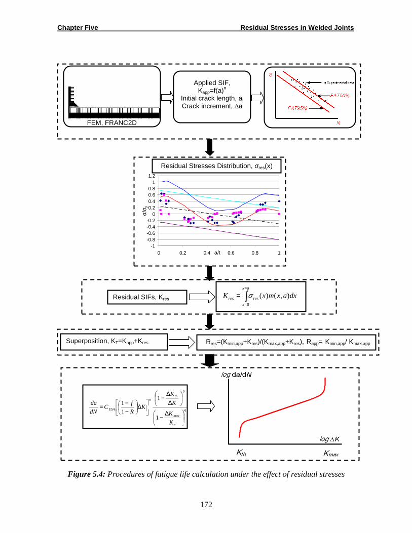
Chapter Five Residual Stresses in Welded Joints
172
sdasa
Figure 5.4: Procedures of fatigue life calculation under the effect of residual stresses
FEM, FRANC2D
-1-0.8-0.6-0.4-0.2
00.20.40.60.8
11.2
0 0.2 0.4 0.6 0.8 1a/t
σ/σ
y
Residual Stresses Distribution, σres(x)
Superposition, KT=Kapp+Kres Rres=(Kmin,app+Kres)/(Kmax,app+Kres), Rapp= Kmin,app/ Kmax,app
Applied SIF, Kapp=f(a)n
Initial crack length, ai
Crack increment, ∆a
Residual SIFs, Kres dxaxmxK
ax
x
resres ),()(0∫=
=
= σ
q
c
max
p
thn
ESA
K
K
K
K
KR
fC
dN
da
∆−
∆∆
−
∆
−−=
1
1
1
1
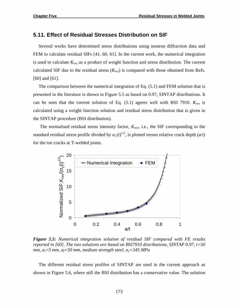
Chapter Five Residual Stresses in Welded Joints
173
5.11. Effect of Residual Stresses Distribution on S IF
Several works have determined stress distributions using neutron diffraction data and
FEM to calculate residual SIFs [41, 60, 61]. In the current work, the numerical integration
is used to calculate Kres as a product of weight function and stress distribution. The current
calculated SIF due to the residual stress (Kres) is compared with those obtained from Refs.
[60] and [61].
The comparison between the numerical integration of Eq. (5.1) and FEM solution that is
presented in the literature is shown in Figure 5.5 as based on 0.97, SINTAP distributions. It
can be seen that the current solution of Eq. (5.1) agrees well with BSI 7910. Kres is
calculated using a weight function solution and residual stress distribution that is given in
the SINTAP procedure (BSI distribution).
The normalised residual stress intensity factor, Knor, i.e., the SIF corresponding to the
standard residual stress profile divided by σy (t)1/2, is plotted versus relative crack depth (a/t)
for the toe cracks at T-welded joints.
0
5
10
15
20
0 0.2 0.4 0.6 0.8 1a/t
Nor
mal
ized
SIF
,Kre
s/(σ
y(t)
1/2 )
Numerical Integration FEM
Figure 5.5: Numerical integration solution of residual SIF compared with FE results reported in [60]. The two solutions are based on BSI7910 distributions, SINTAP 0.97, t=50 mm, ai=5 mm, af=50 mm, medium strength steel, σy=345 MPa
The different residual stress profiles of SINTAP are used in the current approach as
shown in Figure 5.6, where still the BSI distribution has a conservative value. The solution
Chapter Five Residual Stresses in Welded Joints
174
of least square linear fits (Eq. 5.6) is more consistent with experimental data reported in
Ref. [60].
0
2
4
6
8
10
12
0 0.2 0.4 0.6 0.8 1a/t
Nor
mal
ized
SIF
,Kre
s/(σ
y(t)
1/2 )
SINTAP 0.5
Least sequar linear fit
Measured stresses [60]
Figure 5.6: Numerical integration solution of residual SIF compared with that calculated as based on the measured stress distribution for medium strength steel [60] , t=50 mm, ai=5 mm, af=50 mm, medium strength steel, σy=345 MPa
It is shown that the solutions of the current procedure as based on the weight function
and stress distributions agree well with FEA and experimental results that have been
reported in the literature (see Figure 5.6).
The stress intensity factors due to the residual stresses have been calculated using Eq.
(5.1) and FE. In the current work, the ability of both solutions are shown for a/t greater than
0.8.
The FE solution is less conservative and consistent with experimental data. The accuracy
of the current analysis has been verified with experimentally measured data. The
comparison of the Kres for T-plate welded joint calculated from experiments, FE, and by the
current solution is shown in Figure 5.7. The SIF due to residual stresses, Kres increases as
the crack length increases.
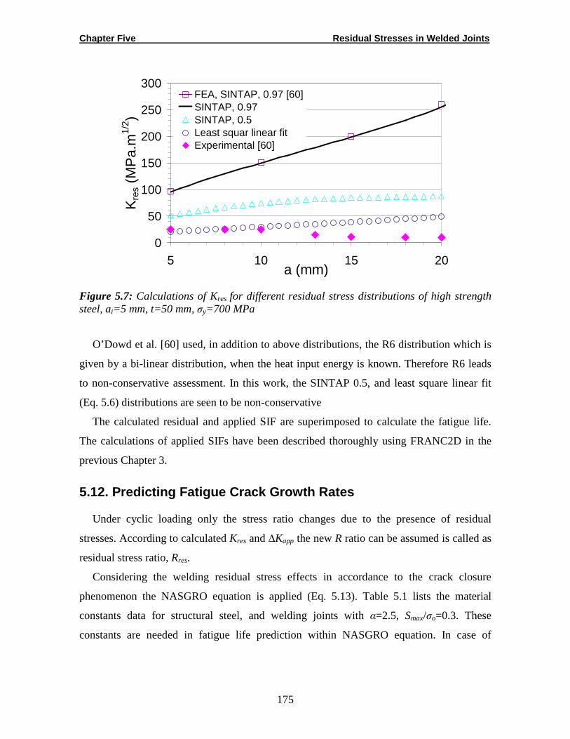
Chapter Five Residual Stresses in Welded Joints
175
0
50
100
150
200
250
300
5 10 15 20a (mm)
Kre
s (M
Pa.
m1/
2 )
FEA, SINTAP, 0.97 [60]SINTAP, 0.97SINTAP, 0.5Least squar linear fitExperimental [60]
Figure 5.7: Calculations of Kres for different residual stress distributions of high strength steel, ai=5 mm, t=50 mm, σy=700 MPa
O’Dowd et al. [60] used, in addition to above distributions, the R6 distribution which is
given by a bi-linear distribution, when the heat input energy is known. Therefore R6 leads
to non-conservative assessment. In this work, the SINTAP 0.5, and least square linear fit
(Eq. 5.6) distributions are seen to be non-conservative
The calculated residual and applied SIF are superimposed to calculate the fatigue life.
The calculations of applied SIFs have been described thoroughly using FRANC2D in the
previous Chapter 3.
5.12. Predicting Fatigue Crack Growth Rates
Under cyclic loading only the stress ratio changes due to the presence of residual
stresses. According to calculated Kres and ∆Kapp the new R ratio can be assumed is called as
residual stress ratio, Rres.
Considering the welding residual stress effects in accordance to the crack closure
phenomenon the NASGRO equation is applied (Eq. 5.13). Table 5.1 lists the material
constants data for structural steel, and welding joints with α=2.5, Smax/σo=0.3. These
constants are needed in fatigue life prediction within NASGRO equation. In case of
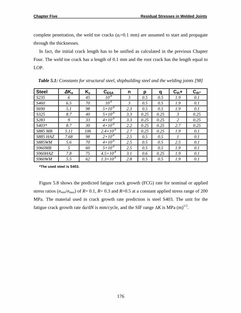
Chapter Five Residual Stresses in Welded Joints
176
complete penetration, the weld toe cracks (ai=0.1 mm) are assumed to start and propagate
through the thicknesses.
In fact, the initial crack length has to be unified as calculated in the previous Chapter
Four. The weld toe crack has a length of 0.1 mm and the root crack has the length equal to
LOP.
Table 5.1: Constants for structural steel, shipbuilding steel and the welding joints [98]
Steel ∆Ko Kc CESA n p q Cth+ Cth- S235 6 45 10-8 3 0.5 0.5 1.9 0.1 S460 6.5 70 10-8 3 0.5 0.5 1.9 0.1 S690 5.1 98 5×10⁻⁸ 2.3 0.5 0.5 1.9 0.1 S325 8.7 40 5×10⁻⁸ 3.3 0.25 0.25 3 0.25 S283 9 33 4×10⁻⁸ 3.3 0.25 0.25 2 0.25 S403* 8.7 30 4×10⁻⁸ 2.2 0.25 0.25 2.7 0.25 S885 MB 5.11 106 2.4×10⁻⁸ 2.7 0.25 0.25 1.9 0.1 S885 HAZ 7.68 98 2×10⁻⁸ 2.5 0.5 0.5 1 0.1 S885WM 5.6 70 4×10⁻⁸ 2.5 0.5 0.5 2.5 0.1 S960MB 5 60 5×10⁻⁸ 2.5 0.5 0.5 1.9 0.1 S960HAZ 7.8 75 4.5×10⁻⁸ 3.1 0.6 0.25 1.9 0.1 S960WM 5.5 62 1.3×10⁻⁸ 2.8 0.5 0.5 1.9 0.1
*The used steel is S403.
Figure 5.8 shows the predicted fatigue crack growth (FCG) rate for nominal or applied
stress ratios (σmin/σmax) of R= 0.1, R= 0.3 and R=0.5 at a constant applied stress range of 200
MPa. The material used in crack growth rate prediction is steel S403. The unit for the
fatigue crack growth rate da/dN is mm/cycle, and the SIF range ∆K is MPa (m)1/2.
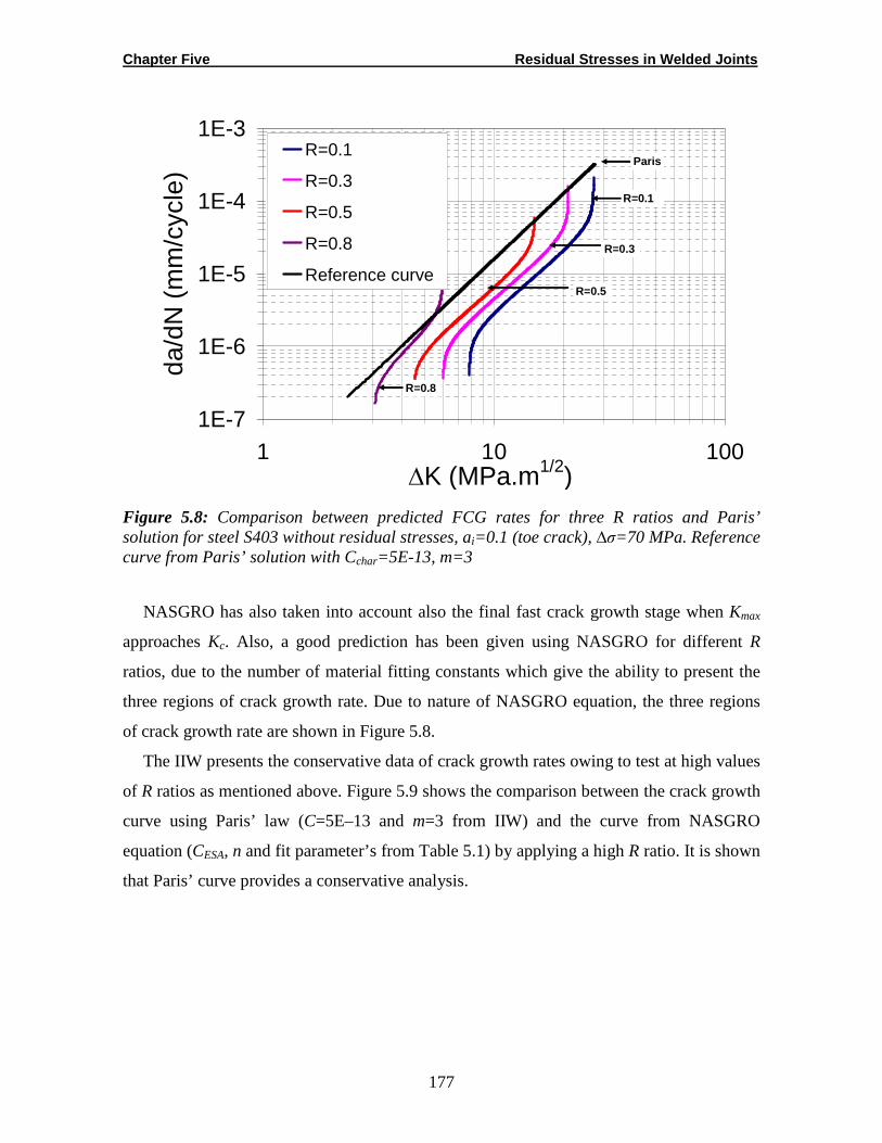
Chapter Five Residual Stresses in Welded Joints
177
1E-7
1E-6
1E-5
1E-4
1E-3
1 10 100∆K (MPa.m1/2)
da/d
N (
mm
/cyc
le)
R=0.1
R=0.3
R=0.5
R=0.8
Reference curve
R=0.1
R=0.3
Paris
R=0.8
R=0.5
Figure 5.8: Comparison between predicted FCG rates for three R ratios and Paris’ solution for steel S403 without residual stresses, ai=0.1 (toe crack), ∆σ=70 MPa. Reference curve from Paris’ solution with Cchar=5E-13, m=3
NASGRO has also taken into account also the final fast crack growth stage when Kmax
approaches Kc. Also, a good prediction has been given using NASGRO for different R
ratios, due to the number of material fitting constants which give the ability to present the
three regions of crack growth rate. Due to nature of NASGRO equation, the three regions
of crack growth rate are shown in Figure 5.8.
The IIW presents the conservative data of crack growth rates owing to test at high values
of R ratios as mentioned above. Figure 5.9 shows the comparison between the crack growth
curve using Paris’ law (C=5E–13 and m=3 from IIW) and the curve from NASGRO
equation (CESA, n and fit parameter’s from Table 5.1) by applying a high R ratio. It is shown
that Paris’ curve provides a conservative analysis.

Chapter Five Residual Stresses in Welded Joints
178
1E-7
1E-6
1E-5
1E-4
1 10 100∆K (MPa.m1/2)
da/d
N (
mm
/cyc
le)
With residual stresses, R=0.8
Paris law
No residual stresses, R=0.8
Figure 5.9: Comparison between two approaches at ∆σ=70 MPa, ai=0.1 mm, t=12 mm. Paris’ constant are Cchar=5E-13 and m=3 [3, 34], S403
It is to be emphasized that the tendency towards an higher crack growth rate in region-III
arises from the influence of static crack extension mechanisms such as micro-cleavage and
void coalescence, where the final failure mechanism is one of cleavage fracture,
contributions to crack growth by micro-cleavage generally occur when Kmax approaches
Kmat (typically Kmax >0.7 Kmat) [107].
5.13. Effect of Residual Stresses and Stress Ratio on FCG Rate
The effect of residual stresses on fatigue crack growth rate (FCG) is accounted by
replacing the nominal R ratio with residual stress ratio Rres. The latter is calculated using the
superposition of applied SIF (Kapp) and SIF due to residual stresses, Kres. NASGRO
considers the effect of plasticity induced crack closure by an empirical constant f as a
function of Rres. In fact, the crack closure phenomenon incorporates the effect of residual
stresses. Therefore, the new Rres will be used within the crack closure ratio, f. More details
have been presented in Chapter Four.
Figure 5.10 shows that the effect of residual stresses on the crack growth rate is
negligible as the applied R ratio increases. This is because the tensile residual stress reduces
the effect of crack closure and increases the crack growth rate. Therefore, for higher applied
Chapter Five Residual Stresses in Welded Joints
179
R ratios, the influence of residual stresses on growth rate is small because the crack remains
open throughout the whole cycle.
The effect of stress ratio can be discussed by the effect of crack closure mechanism. This
mechanism is related to the crack path meanders. It is important to explain stress ratio
effects in connection with residual stresses as shown in Figure 5.10 in terms of mode-I
stress intensity factor range ∆KI. At higher R-values, the curves of da/dN (Figure 5.10a-e)
differ from each other substantially in the threshold region, showing a typical stress ratio
effect.
1E-7
1E-6
1E-5
1E-4
1E-3
1 10 100∆K (MPa.m1/2)
da/d
N (
mm
/cyc
le)
With residual stresses, R=0.1
No residual stresses, R=0.1
(a)
1E-7
1E-6
1E-5
1E-4
1E-3
1 10 100∆K (MPa.m1/2)
da/d
N (
mm
/cyc
le)
With residual stresses, R=0.3
No residual stresses, R=0.3
(b)
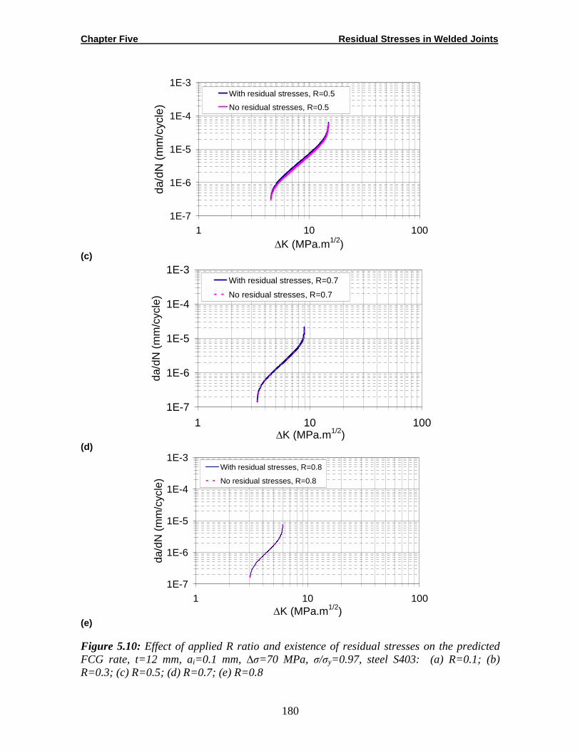
Chapter Five Residual Stresses in Welded Joints
180
1E-7
1E-6
1E-5
1E-4
1E-3
1 10 100∆K (MPa.m1/2)
da/d
N (
mm
/cyc
le)
With residual stresses, R=0.5
No residual stresses, R=0.5
(c)
1E-7
1E-6
1E-5
1E-4
1E-3
1 10 100∆K (MPa.m1/2)
da/d
N (
mm
/cyc
le)
With residual stresses, R=0.7
No residual stresses, R=0.7
(d)
1E-7
1E-6
1E-5
1E-4
1E-3
1 10 100∆K (MPa.m1/2)
da/d
N (
mm
/cyc
le)
With residual stresses, R=0.8
No residual stresses, R=0.8
(e)
Figure 5.10: Effect of applied R ratio and existence of residual stresses on the predicted FCG rate, t=12 mm, ai=0.1 mm, ∆σ=70 MPa, σ/σy=0.97, steel S403: (a) R=0.1; (b) R=0.3; (c) R=0.5; (d) R=0.7; (e) R=0.8
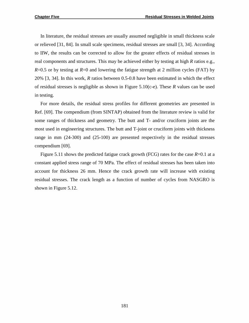
Chapter Five Residual Stresses in Welded Joints
181
In literature, the residual stresses are usually assumed negligible in small thickness scale
or relieved [31, 84]. In small scale specimens, residual stresses are small [3, 34]. According
to IIW, the results can be corrected to allow for the greater effects of residual stresses in
real components and structures. This may be achieved either by testing at high R ratios e.g.,
R=0.5 or by testing at R=0 and lowering the fatigue strength at 2 million cycles (FAT) by
20% [3, 34]. In this work, R ratios between 0.5-0.8 have been estimated in which the effect
of residual stresses is negligible as shown in Figure 5.10(c-e). These R values can be used
in testing.
For more details, the residual stress profiles for different geometries are presented in
Ref. [69]. The compendium (from SINTAP) obtained from the literature review is valid for
some ranges of thickness and geometry. The butt and T- and/or cruciform joints are the
most used in engineering structures. The butt and T-joint or cruciform joints with thickness
range in mm (24-300) and (25-100) are presented respectively in the residual stresses
compendium [69].
Figure 5.11 shows the predicted fatigue crack growth (FCG) rates for the case R=0.1 at a
constant applied stress range of 70 MPa. The effect of residual stresses has been taken into
account for thickness 26 mm. Hence the crack growth rate will increase with existing
residual stresses. The crack length as a function of number of cycles from NASGRO is
shown in Figure 5.12.
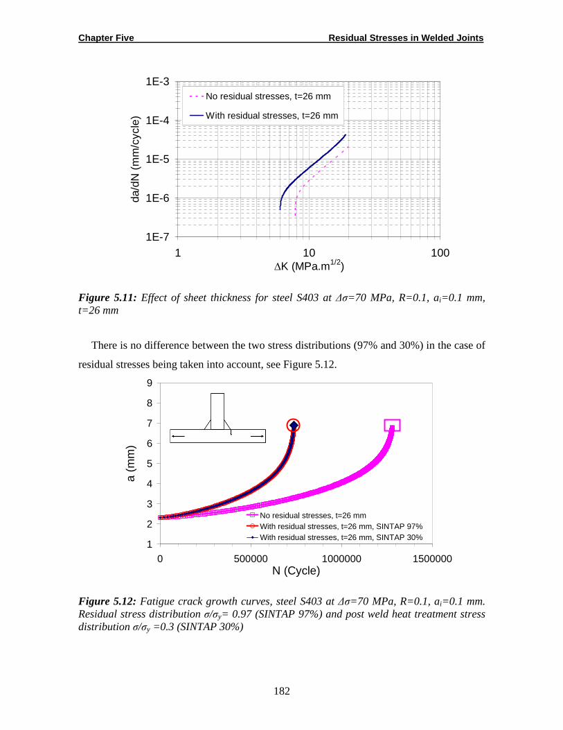
Chapter Five Residual Stresses in Welded Joints
182
1E-7
1E-6
1E-5
1E-4
1E-3
1 10 100∆K (MPa.m1/2)
da/d
N (
mm
/cyc
le)
No residual stresses, t=26 mm
With residual stresses, t=26 mm
Figure 5.11: Effect of sheet thickness for steel S403 at ∆σ=70 MPa, R=0.1, ai=0.1 mm, t=26 mm
There is no difference between the two stress distributions (97% and 30%) in the case of
residual stresses being taken into account, see Figure 5.12.
1
2
3
4
5
6
7
8
9
0 500000 1000000 1500000N (Cycle)
a (m
m)
No residual stresses, t=26 mmWith residual stresses, t=26 mm, SINTAP 97%With residual stresses, t=26 mm, SINTAP 30%
Figure 5.12: Fatigue crack growth curves, steel S403 at ∆σ=70 MPa, R=0.1, ai=0.1 mm. Residual stress distribution σ/σy= 0.97 (SINTAP 97%) and post weld heat treatment stress distribution σ/σy =0.3 (SINTAP 30%)
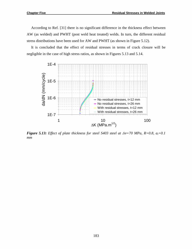
Chapter Five Residual Stresses in Welded Joints
183
According to Ref. [31] there is no significant difference in the thickness effect between
AW (as welded) and PWHT (post weld heat treated) welds. In turn, the different residual
stress distributions have been used for AW and PWHT (as shown in Figure 5.12).
It is concluded that the effect of residual stresses in terms of crack closure will be
negligible in the case of high stress ratios, as shown in Figures 5.13 and 5.14.
1E-7
1E-6
1E-5
1E-4
1 10 100∆K (MPa.m1/2)
da/d
N (
mm
/cyc
le)
No residual stresses, t=12 mmNo residual stresses, t=26 mmWith residual stresses, t=12 mmWith residual stresses, t=26 mm
Figure 5.13: Effect of plate thickness for steel S403 steel at ∆σ=70 MPa, R=0.8, ai=0.1 mm
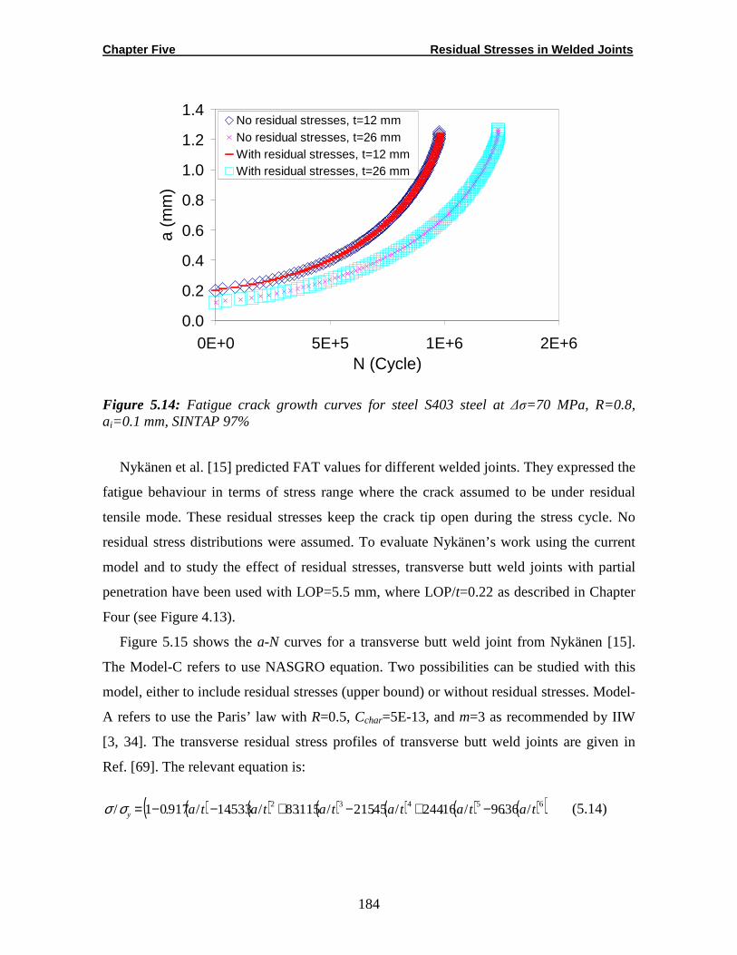
Chapter Five Residual Stresses in Welded Joints
184
0.0
0.2
0.4
0.6
0.8
1.0
1.2
1.4
0E+0 5E+5 1E+6 2E+6N (Cycle)
a (m
m)
No residual stresses, t=12 mmNo residual stresses, t=26 mmWith residual stresses, t=12 mm With residual stresses, t=26 mm
Figure 5.14: Fatigue crack growth curves for steel S403 steel at ∆σ=70 MPa, R=0.8, ai=0.1 mm, SINTAP 97%
Nykänen et al. [15] predicted FAT values for different welded joints. They expressed the
fatigue behaviour in terms of stress range where the crack assumed to be under residual
tensile mode. These residual stresses keep the crack tip open during the stress cycle. No
residual stress distributions were assumed. To evaluate Nykänen’s work using the current
model and to study the effect of residual stresses, transverse butt weld joints with partial
penetration have been used with LOP=5.5 mm, where LOP/t=0.22 as described in Chapter
Four (see Figure 4.13).
Figure 5.15 shows the a-N curves for a transverse butt weld joint from Nykänen [15].
The Model-C refers to use NASGRO equation. Two possibilities can be studied with this
model, either to include residual stresses (upper bound) or without residual stresses. Model-
A refers to use the Paris’ law with R=0.5, Cchar=5E-13, and m=3 as recommended by IIW
[3, 34]. The transverse residual stress profiles of transverse butt weld joints are given in
Ref. [69]. The relevant equation is:
( ) ( ) ( ) ( ) ( ) ( )( )65432 /36.96/16.244/45.215/115.83/533.14/917.01/ tatatatatatay −+−+−−= σσ (5.14)
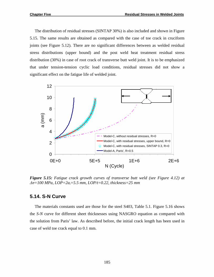
Chapter Five Residual Stresses in Welded Joints
185
The distribution of residual stresses (SINTAP 30%) is also included and shown in Figure
5.15. The same results are obtained as compared with the case of toe crack in cruciform
joints (see Figure 5.12). There are no significant differences between as welded residual
stress distributions (upper bound) and the post weld heat treatment residual stress
distribution (30%) in case of root crack of transverse butt weld joint. It is to be emphasized
that under tension-tension cyclic load conditions, residual stresses did not show a
significant effect on the fatigue life of welded joint.
0
2
4
6
8
10
12
0E+0 5E+5 1E+6 2E+6N (Cycle)
a (m
m)
Model-C, without residual stresses, R=0
Model-C, with residual stresses, upper bound, R=0
Model-C, with residual stresses, SINTAP 0.3, R=0
Model-A, Paris', R=0.5
Figure 5.15: Fatigue crack growth curves of transverse butt weld (see Figure 4.12) at ∆σ=100 MPa, LOP=2ai=5.5 mm, LOP/t=0.22, thickness=25 mm
5.14. S-N Curve
The materials constants used are those for the steel S403, Table 5.1. Figure 5.16 shows
the S-N curve for different sheet thicknesses using NASGRO equation as compared with
the solution from Paris’ law. As described before, the initial crack length has been used in
case of weld toe crack equal to 0.1 mm.
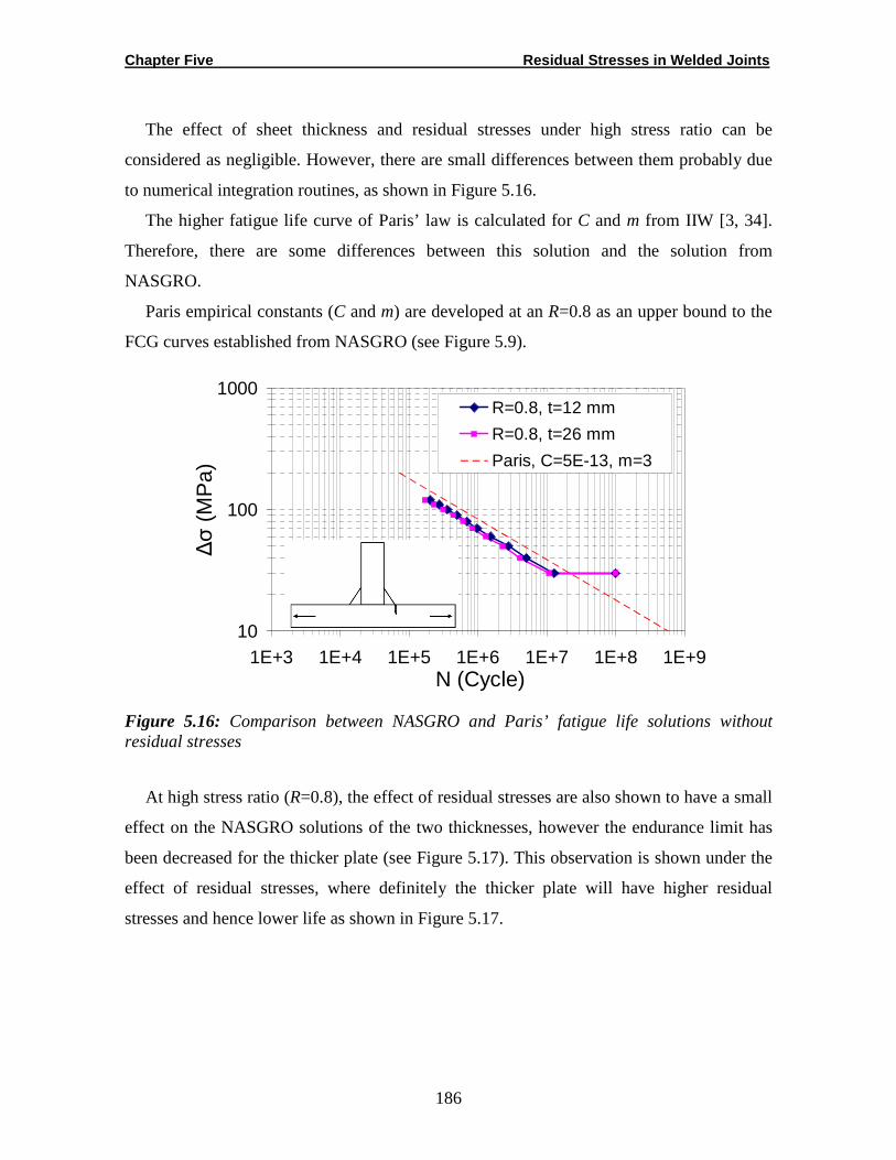
Chapter Five Residual Stresses in Welded Joints
186
The effect of sheet thickness and residual stresses under high stress ratio can be
considered as negligible. However, there are small differences between them probably due
to numerical integration routines, as shown in Figure 5.16.
The higher fatigue life curve of Paris’ law is calculated for C and m from IIW [3, 34].
Therefore, there are some differences between this solution and the solution from
NASGRO.
Paris empirical constants (C and m) are developed at an R=0.8 as an upper bound to the
FCG curves established from NASGRO (see Figure 5.9).
10
100
1000
1E+3 1E+4 1E+5 1E+6 1E+7 1E+8 1E+9N (Cycle)
∆σ
(M
Pa)
R=0.8, t=12 mm
R=0.8, t=26 mm
Paris, C=5E-13, m=3
Figure 5.16: Comparison between NASGRO and Paris’ fatigue life solutions without residual stresses
At high stress ratio (R=0.8), the effect of residual stresses are also shown to have a small
effect on the NASGRO solutions of the two thicknesses, however the endurance limit has
been decreased for the thicker plate (see Figure 5.17). This observation is shown under the
effect of residual stresses, where definitely the thicker plate will have higher residual
stresses and hence lower life as shown in Figure 5.17.
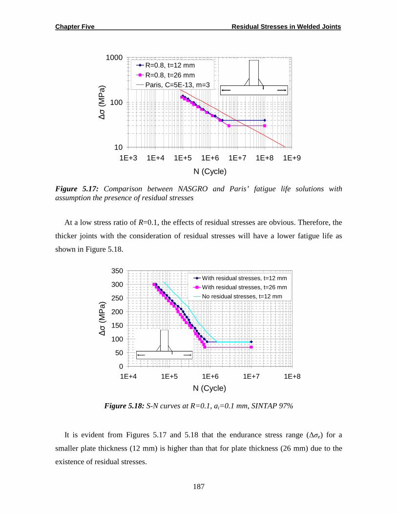
Chapter Five Residual Stresses in Welded Joints
187
10
100
1000
1E+3 1E+4 1E+5 1E+6 1E+7 1E+8 1E+9
N (Cycle)
∆σ
(M
Pa)
R=0.8, t=12 mmR=0.8, t=26 mmParis, C=5E-13, m=3
Figure 5.17: Comparison between NASGRO and Paris’ fatigue life solutions with assumption the presence of residual stresses
At a low stress ratio of R=0.1, the effects of residual stresses are obvious. Therefore, the
thicker joints with the consideration of residual stresses will have a lower fatigue life as
shown in Figure 5.18.
0
50
100
150
200
250
300
350
1E+4 1E+5 1E+6 1E+7 1E+8
N (Cycle)
∆σ
(M
Pa)
With residual stresses, t=12 mm
With residual stresses, t=26 mm
No residual stresses, t=12 mm
Figure 5.18: S-N curves at R=0.1, ai=0.1 mm, SINTAP 97%
It is evident from Figures 5.17 and 5.18 that the endurance stress range (∆σe) for a
smaller plate thickness (12 mm) is higher than that for plate thickness (26 mm) due to the
existence of residual stresses.
Chapter Five Residual Stresses in Welded Joints
188
5.15. Conclusions
Most studied have neglected the effect of residual stresses in small thickness scale. In
this work a numerical integration program is established to calculate SIFs due to residual
stresses (Kres) which is a product of traditional weight function and residual stress
distributions through the thickness of the plate. The transverse residual stresses have a
major effect on the crack growth through the thickness of joints. Two transverse residuals
stress distributions away from the weld toe and from LOP are used for the plate T-butt weld
and for plate butt welds. For conservative results, the upper bound residual distributions are
used in this work. For evolution purpose, the other distributions are examined.
The residual stress distributions which are given in the recommendations are used in the
current procedures and compared with literature. Due to limiting use of weight function,
most literature has used the residual stress distributions from experimental measurements
(neutron diffraction) and FEM to calculate Kres. In this work, the calculations which are
based on the weight function and available distributions to calculate Kres and lives are
satisfactory.
Since the weight function is used for a pre-existing crack, the application of this function
method to the crack propagation analysis step by step with the presence of a residual stress
field is yet to be carried out.
The solution of SIF due to the residual stress (Kres) from the product of weight function
and SINTAP residual stress distributions have been compared with those obtained from
FEM-based methods and measured experimental data. The comparisons show a good
agreement. Therefore, the ability to use the weight function higher than the restricted limits
which were mentioned before (a/t=0.5) is demonstrated.
The phenomenon of the change of the residual stresses during fatigue cycle is
investigated in correlation with the applied load ratio using the superposition method. In
this work, the superposition of residual stresses in the calculation of total SIF is used.
Although this method has been criticized by other researchers, the results which were
obtained are quite well.
An increasing R ratio will reduce the effect of residual stresses on the predicted life
because the higher tensile residual stresses reduce the effect of crack closure, i.e., the crack
Chapter Five Residual Stresses in Welded Joints
189
remains open. Therefore, for higher R ratios, the influence of residual stresses and Kres on
the growth rate is small. Important stress ratio effects appear in the threshold region, where
∆Kth decreases as R increases.
The comparisons with literature in case of residual stresses are presented in this chapter.
Different distribution ratios were used for this comparison, e.g. σ/σy=0.97%, 0.5% and
0.3%.
Finally, the effects of joints geometry and materials properties can be studied according
to the current approach.
Chapter Six Conclusions and Recommendations for Future Work
190
Chapter Six
CONCLUSIONS AND RECOMMENDATIONS FOR
FUTURE WORK
6.1. Conclusions
This work has three main parts: in the first part, the stress intensity factor (SIF) is
calculated and evaluated; in the second part the SIF is used in the calculations of fatigue
life; and by using suitable life formula, backward calculations using the built language
program were carried out to determine the critical crack sizes (ai, and af), and fatigue
strength (FAT). The fatigue life calculations with the effect of residual stresses are
described in the third part.
Even though there are many studies dealing with fracture mechanics, this thesis
combines FEA with fracture mechanics to develop a simple and reliable procedure to
predict fatigue life of welded joints on basis of fatigue crack growth. The used approach
works within the assumptions of linear elastic fracture mechanics (LEFM). The adopted
method assumes a crack existing at an edge of welded joints. After this crack starts to grow,
it will be under the normal applied tensile stress (maximum stress criterion). Hence, the
effect of plasticity will be small when the opening mode dominates. Therefore, the
assumption of LEFM is reasonable.
Fatigue life calculations of welded joints with different combinations of geometrical
parameters have been carried out using the results of SIFs that were obtained from FEM.
These SIF results are evaluated, benchmarked and compared with available solutions. New
SIF solutions have been developed then.
The simulation of fatigue crack propagation and SIF calculations using FEM is found to
be effective to determine the fatigue strength (FAT) and establishing the S-N curve.
Chapter Six Conclusions and Recommendations for Future Work
191
Experimental data from literature are used to verify the current approach including the
effects of weld geometries and residual stresses.
The fatigue life and SIFs of load-carrying joints with various weld shapes have been
accurately estimated by performing a fatigue crack propagation analysis when the crack is
originated from the weld root of the joint or from the lack of penetration (LOP),
respectively. In contrast, the fatigue life of non-load-carrying joints is investigated with the
presence of the weld toe crack.
Although real components are often different from the details contemplated in the
standards, successful comparisons are carried out with experimental data. Moreover, this
work investigates the effect of some welded geometrical parameters and residual stresses
on the propagation life of welded joints. Verifications of FAT classes from standers are also
carried out.
To carry out the integration of the fatigue life equation (e.g., Paris or NASGRO),
accurate values of initial crack length, and final crack length with a fixed crack growth
parameters (C and m) are required. The values of cracks length are determined and
compared with experimental data. A value of the initial crack length of 0.1 mm is shown to
be a typical length for the case of weld toe crack. Longer crack lengths are determined in
the case of a root crack where the crack length is equal to the size of the non-welded area
(LOP).
Although there are considerable fatigue data for welded joins for steel and aluminum in
recommendations such as IIW and BSI, the problem exists to find the fatigue strength data
for some other materials. In that case, the sparse design data for welded joints for different
materials can be calculated easily with the current work.
The results are then used to indicate the initial weld sizes which would be necessary to
avoid failure on the weld throat (case of LOP) and on the base plate (case of toe crack).
Therefore, the entire fatigue life is assumed to be crack propagation.
As expected, increasing the size of the lack of penetration will increase the probability of
weld throat crack propagation and will decrease the fatigue life absolutely. Also, the
increasing weld size will decrease the FAT value.
Verification of the current results is reported during the comparisons with experimental
data. Moreover, the comparisons with predicted FAT-class from Ref. [15] are presented.

Chapter Six Conclusions and Recommendations for Future Work
192
The recommendation to use the current approach parameters will take an advantage,
because SIFs and ai are only needed to find an appropriate FAT for different geometries.
The crack propagation of two cracks at same time has different criteria for estimation the
crack life, i.e., determination which crack will contribute to final failure, or if both will
contribute in final failure. The faster crack will propagate according to throat thickness
geometry and applied load nature.
Residual stresses have an effect on fatigue crack propagation. The residual stress
distributions are studied and compared with the experimental data. Therefore, SIFs due to
residual stresses are calculated from the product of weight function and residual stress
distributions at the crack tip. The universal weight function was used in this analysis.
These calculations we carried out step by step for each cycle and each crack increment.
Residual stress ratios were calculated as a function of the residual SIF (Kres) that were
calculated from the weight function method and applied SIF (Kapp) that in turn were
calculated from FEM. The combination of residual stress ratio and applied stress ratio with
residual stress effects are shown to be less investigated and unexplained in the literature for
fillet welded joints.
This work has shown this combination which gives in turn the crack propagation under
the effect of residual stresses. The main finding is that the effect of residual stresses and
sheet thickness are ignorable when the stress ratio is more than R=0.5. In the case of lower
stress ratio (R=0.1), a lower sheet thickness will have a higher fatigue strength. These
results also reveal that the residual stresses increase with increasing the component
thickness due to the increase in the heat input of the welding in the real workshop, which in
reality means that a larger thickness will have a temperature gradient that increases the
residual stresses.
6.2. The Originality of the Dissertation
Although, the application of ordinary fracture mechanics parameters like K to very small
cracks is not appropriate (particularly in fatigue and short crack growth), this work presents
good results according to LEFM. The original parts from this thesis are summarized by the
following points:

Chapter Six Conclusions and Recommendations for Future Work
193
1. Examination the crack path effects on SIF solution and in turn it’s effect on fatigue life.
Therefore, the difference between the SIF-solutions from IIW, BSI and current work has
been presented and their effect on S-N is shown. Then the effect of meandering cracks is
taken into account.
2. Determined analytically the crack’s lengths which seriously effect joints strength and
lead to catastrophic failure. Moreover, these lengths are evaluated as compared with
experimental data. Typical crack lengths were determined according to the joint’s
geometry, crack’s type and locations. Initial crack length equal to 0.1 mm and LOP are
satisfied in case of toe and root crack respectively. Final crack length and crack increment
also verified. In previous works, these lengths are presented mostly as a range of length or
they have been assumed [15].
3. Determined the fatigue strength and life of unknown cases. The validations of FAT-
values are examined for different notch joints. Also the effects of joints geometry such as
plate thickness are investigated. The explanation of the thickness effect using the current
work is presented according to fracture mechanics and FE point of view. Then, the effect of
constant crack length and scaling crack length with respect to thickness is presented.
4. The effects of weld notch geometry were investigated as well as their effect of FAT-
value.
5. Calculated analytically the SIF due to residual stresses which previously calculated
either from experimental measurements of residual stress distributions, or from FEM.
6. The combination of two R-ratios (residual and applied stress ratio), and calculating SIF
due to residual stresses for each crack step have not yet been sufficiently investigated. In
addition, these calculations were repeating at crack tip for each crack increment.
7. An increasing R ratio will reduce the effect of residual stresses on the predicted life
because the higher tensile residual stresses reduce the effect of crack closure, i.e., the crack
remains open. Therefore, for higher R ratios, the influence of residual stresses and Kres on
the growth rate is small. Important stress ratio effects appear in the threshold region, ∆Kth
decrease as R increase.
8. The comparison with Nykänen’s work shows that there is an effect of residual stresses
distributions and stress ratio.
Chapter Six Conclusions and Recommendations for Future Work
194
9. The stress concentration factor can be calculated from predicted FAT-values. Then the
machined weld overfills give higher fatigue resistance.
6.3. Recommendations for Future Work
For time and experiments constraints and according to the lack found in the related
literature, some works are recommended for future work such as:
1. No standards are presently available for welded components made of other materials
(e.g. titanium alloys, etc.). The current fracture mechanics approach can be applied for
other materials.
2. Investigation of other welded joints’ geometries and calculation the FAT values for
layered joints such as spot welded joints.
3. Simulation of the various types of defects within the weld using the current approach.
These defects might have an effect on the calculated value of the crack length. Therefore, a
new systematic set of values and relationships can be developed.
4. Studying the validity of the currently calculated parameters (C, m, ai, af, FAT and S-N
curve) with other loading types.
5. Studying the validity of the currently calculated parameters under the effect of
environment, e.g., corrosion effect, temperature and cryogenic effect.
6. Establishing a criterion to forecast the possible crack initiation and propagation region
(toe or root) in the welded joints which have these two types of cracks, i.e., determine the
faster effecting crack causing the final failure. Also to determine the probable FAT and S-N
curve.
References
195
REFERENCES
[1] Lassen T., and Recho N., Fatigue Life Analyses of Welded Structures, ISTE Ltd, 2006.
[2] Blondeau R., Metallurgy and Mechanics of Welding, ISTE Ltd, 2008.
[3] Hobbacher A., Recommendations for Fatigue Design of Welded Joints and Components, IIW Doc., No XIII-1965r14-03 / XV-1127r14-03, International Institute of Welding, 2006
[4] Branco C.M., Maddox S.J., Infante V. and Gomes E.C., Fatigue Performance of Tungsten Inert Gas (TIG) and Plasma Welds in Thin Sections, International Journal of Fatigue, Vol. 21, No. 6, pp. 587–601, 1999.
[5] Barsoum Z. and Barsoum I., Residual Stress Effects on Fatigue Life of Welded Structures Using LEFM, Engineering Failure Analysis, Vol. 16, No. 1, pp. 449–467, 2009.
[6] Nagaralu R., Fatigue Crack Growth under Residual Stress around Holes, Mississippi State University, M.Sc. Thesis, USA, 2005.
[7] Andersen M.R., Fatigue Crack Initiation and Growth in Ship Structures, Ph.D. Thesis, Technical University of Denmark, Denmark, 1998.
[8] Alam M.S., Structural Integrity and Fatigue Crack Propagation Life Assessment of Welded and Weld-Repaired Structures, Ph.D. Dissertation, Louisiana State University, USA, 2005.
[9] Webster G.A., and Ezeilo A.N., Residual Stress Distribution and Their Influence on Fatigue Life Times, International Journal of Fatigue, Vol. 23, No. 1, pp. s375–s383, 2001.
[10] Fukuda S. and Tsuruta Y., An Experimental Study of Redistribution of Welding Residual Stress with Fatigue Crack Extension, Transaction of JWRI, Vol. 7, No. 2, pp. 67–72, 1978.
[11] Lampeas G.N. and Diamantakos I.D., Calculation of Stress Intensity Factors of Cracked T-Joints Considering Laser Beam Welding Residual Stresses, First International Conference on Damage Tolerance of Aircraft Structures, TU Delft, The Netherlands, September 25–28, 2007.
[12] Eurocode 3, Design of Steel Structures, 1990.
[13] Germanischer Lloyd Aktiengesellschaft, Rules for Classification and Construction, Part I Ship Technology, Section 20C, Fatigue strength, Germanischer Lloyd Aktiengesellschaft, GL 2007, <www.gl-group.com>.
[14] British Standards Institution, Guidance on Methods for the Acceptance of Flaws in Structure, PD 6493, BS 7910, Appendix J, 2005.

References
196
[15] Nykänen T., X. Li, Björk T. and Marquis G., A Parametric Fracture Mechanics Study of Welded Joints with Toe Cracks, Engineering Fracture Mechanics, Vol. 72, No. 10, pp. 1580–1609, 2005.
[16] Smith I.F.C. and Smith R.A., Fatigue Crack Growth in a Fillet Welded Joints, Engineering Fracture Mechanics, Vol. 18, No. 4, pp. 861-869, 1983.
[17] Testin R.A., Yung J.Y., Lawrence F.V. and Rice R.C., Predicting the Fatigue Resistance of Steel Weldments, Weld. Res. Suppl., Vol. 4, pp. 93–98, 1987.
[18] Ferreira J.M. and Branco C.M., Influence of Fillet Weld Joint Geometry on Fatigue Crack Growth, Theoretical and Applied Fracture Mechanics, Vol. 15, pp. 131–142, 1991.
[19] Motarjemi A.K., Kokabi A.H., Ziaie A.A., Manteghi S. and Burdekin F.M., Comparison of the Stress Intensity Factor of T and Cruciform Welded Joints with Different Main and Attachment Plate Thickness, Engineering Fracture Mechanics, Vol. 65, No. 1, pp. 55–66, 2000.
[20] Balasubramanian V. and Guha B., Fatigue Life Predication of Welded Cruciform Joints Using Strain Energy Density Factor Approach, Theoretical and Applied Fracture Mechanics, Vol. 34, No. 1, pp. 85–92. 2000.
[21] Frank K.H. and Fisher J.W., Fatigue Strength of Fillet Welded Cruciform Joints, J. Struct. Division, ASCE, 105(ST9), pp. 1727–1740, 1979.
[22] Usami S. and Kusumoto S., Fatigue Strength at Roots of Cruciform, Tee and Lap Joints, Transactions of Japan Welding Society, Vol. 9, No. 1, pp. 1–10, 1979.
[23] Caccese V., Blomquist P.A., Berube K.A, Webber S.R. and Orozco N.J., Effect of Weld Geometric Profile on Fatigue Life Cruciform Welds Made by Laser/GMAW Processes, Marine Structure, Vol. 19, No. 1, pp. 1–22, 2006.
[24] Teng T.-L., Fung C.-P. and Chang P.-H., Effect of Weld Geometry and Residual Stress on Fatigue in Butt-Welded Joints, International Journal of Pressure Vessels and Piping, Vol. 79, No. 7, pp. 467–482, 2002.
[25] Mashiri F.R., Zhao X.L. and Grundy P., Effect of Weld Profile and Undercut on
Fatigue Crack Propagation Life of Thin Walled Cruciform Joint, Thin Walled Structures, Vol. 39, No. 3, pp. 261–285, 2001.
[26] Maddox S.J., An Analysis of Fatigue Cracks in Fillet Welded Joints, International Journal of Fracture, Vol. 11, No. 2, pp. 221–243, 1975.
[27] Metrovich B., Fisher J.W., Yen B.T., Kaufmann E.J., Cheng X. and Ma Z., Fatigue Strength of Welded AL-6XN Superaustenitic Stainless Steel, International Journal of Fatigue, Vol. 25, No. 9, pp. 1309–1315, 2003.
References
197
[28] Wu W., Fatigue Crack Propagation Behavior of Welded and Weld Repaired 5083 Aluminum Alloy Joints, M.Sc. Thesis, School of Aerospace and Mechanical Engineering, The University of New South Wales, Australia, 2002.
[29] Poutiainen I. and Marquis G., A Fatigue Assessment Method Based on Weld Stress, International Journal of Fatigue, Vol. 28, No. 9, pp. 1037–1046, 2006.
[30] Engesvik K., Analysis of the Uncertainty of the Fatigue Capacity of Welded Joints, NTNU, Trondheim, UR-82-17, Norway, 1983.
[31] Lindqvist J., Fatigue Strengths Thickness Dependence in Welded Construction, M.Sc. Thesis, Borlänge, Sweden, 2002.
[32] Karlsson N. and Lenanader P.-H., Analysis of Fatigue Life in Two Welded Class System, M.Sc. Thesis, LITH-IKP-EX—05/2302-SE, Department of Mechanical Engineering, Linköping University, Sweden, 2005.
[33] Hobbacher A., Stress Intensity Factors of Welded Joints, Engineering Fracture Mechanics, Vol. 46, No. 2, pp. 173–182, 1993.
[34] Hobbacher A., Recommendations for Fatigue Design of Welded Joints and Components, IIW document XIII-2151-07 / XV-1254-07, International Institute of Welding - IIW / IIS, 2007.
[35] Maddox S.J., Fatigue of Welded Joints, Seminar on Fatigue Performance of Weldments, The Welding Institute, Cambridge, England, 1983.
[36] Samuelsoon J., Integrated Design and Manufacturing of Welded Structures, Nordic Innovation Center, Norway, 2007.
[37] Nguyen N.T. and Wahab M.A., The Effect of Residual Stresses and Weld Geometry on the Improvement of Fatigue Life, Journal of Materials Processing Technology, Vol. 48, pp. 581–588, 1995.
[38] Singh P.J., Guha B. and Achar D.R.G., Fatigue Life Improvement of AISI 304L Cruciform Welded Joints by Cryogenic Treatment, Engineering Failure Analysis, Vol. 10, No. 1, pp 1–12, 2003.
[39] Hou C.-Y. and Charng J.-J., Models for the Estimation of Weldemnt Fatigue Crack Initiation Life, International Journal of Fatigue, Vol. 19, No. 7, pp. 537–541, 1997.
[40] Stoyan S., Kujawski D. and Mallory J., Fatigue Crack Growth in 2324 Aluminum Alloy, Western Michigan University, Technical Report No. MAE-05-01, 2005.
[41] Guo K., Bell R. and Wang X., The Stress Intensity Factor Solutions for Edge Cracks in a Padded Plate Geometry under General Loading Conditions, International Journal of Fatigue, Vol. 29, pp. 481–488, 2007.
References
198
[42] Bäckström M., Multi Axial Fatigue Life Assessment of Welds Based on Nominal and Hot Spot Stress, Ph.D. Thesis, Lappeenranta University of Technology, Lappeenranta, Finland, 2003.
[43] BEASY, <http://www.beasy.com>.
[44] Fricke W., Doerk O. and Grünitz L., Fatigue Strength Investigation and Assessment of Fillet Welds around Stiffener and Bracket Toes, Proceedings of OMAE specialty symposium on FPSO integrity, Houston, 2004.
[45] Fricke W. and Doerk O., Simplified Approach to Fatigue Strength Assessment of Fillet-Welded Attachment Ends, International Journal of Fatigue, Vol. 28, No. 2, pp. 141–150, 2006.
[46] Cornell Fracture Group, FRANC2D Version 3.2, <http://www.cfg.cornell.edu>.
[47] Hee S.C. and Jefferson A.D., Two-Dimensional Analysis of a Gravity Dam Using the Program Franc2D, Cardiff University, U.K., 2005.
[48] Ferrica J.A. and Branco C.M., Fatigue Analysis and Prediction in Filled Welded Joints in the Low Thickness Range, Fatigue and Fracture Engineering Materials and Structures, Vol. 13, No. 3, pp. 201–212, 1990.
[49] Kainuma S. and Mori T., A Fatigue Strength Evaluation Method for Load-Carrying Fillet Welded Cruciform Joints, International Journal of Fatigue, Vol. 28, No. 8, pp. 864–872, 2006.
[50] Nguyen N.T. and Wahab M.A., A Theoretical Study of the Effect of Weld Geometry Parameters on Fatigue Crack Propagation Life, Journal of Engineering Fracture Mechanics, Vol. 51, No. I, pp. 1–18, 1995.
[51] Ohta M.T. and Suzuki N., Evaluation of Effect of Plate Thickness on Fatigue Strength of Butt Welded Joints by a Test Maintaining Maximum Stress at Yield Strength, Engineering Fracture Mechanics, Vol. 37, No. 5, pp. 987–993, 1990.
[52] Bimalendu G., Effect of Specimen Geometry on Fatigue of Welded Joints, Engineering Fracture Mechanics, Vol. 46, No. 1, pp. 35–39, 1993.
[53] Niu X. and Glinka G., The Weld Profile Effect on Stress Intensity Factors in Weldments, International Journal of Fracture, Vol. 35, No.1, pp. 3–20, 1987.
[54] Motarjemi A.K., Kokabi A.H. and Burdekin F.M., Comparison of Fatigue Life for T and Cruciform Welded Joints with Different Combinations of Geometrical Parameters, Engineering Fracture Mechanics, Vol. 67, No. 4, pp. 311–326, 2000.
[55] Taylor D., Barrett N. and Lucano G., Some New Method for Prediction Fatigue in Welded Joint, International Journal of Fatigue, Vol. 24, No. 5, pp. 509–518, 2002.
References
199
[56] National Institute of Materials Science (NIMS), Data Sheet on Fatigue Properties of Non-Load-Carrying of Cruciform Welded Joints of SM490B Rolled Steel for Welded Structure-Effect of Plate Thickness (Part 3, Thickness 80 mm), Fatigue Data Sheet, No. 108, Japan, 2009.
[57] Radhakrishnan V.M., Welding Technology and Design, 2nd edition, New Age International Publishers, 2007.
[58] Itoh Y.Z., Suruga S. and Kashiwaya H., Prediction of Fatigue Crack Growth Rate in Welding Residual Stress Field, Engineering Fracture Mechanics, Vol. 33, No. 3, pp. 397–407, 1989.
[59] Barsoum Z., Residual Stress Analysis and Fatigue Assessment of Welded Steel
Structures, Ph.D. Thesis, KTH Engineering Science, Sweden, 2008.
[60] O’Dowd N.P., Nikbin K.M., Lee H.-Y., Wimpory R. C. and Biglari F.R., Stress Intensity Factors due to Residual Stresses in T-Plate Welds, Journal of Pressure Vessel and Technology, Transactions of the ASME, Vol. 126, pp. 432–437, 2004.
[61] Lee H.-Y., Biglari F.R., Wimpory R. and Nikbin K.M., Treatment of Residual Stress in Failure Assessment Procedure, Engineering Fracture Mechanics, Vol. 73, No. 13, pp. 1755–1771, 2006.
[62] Assis J.T., Monin V., Teodosio J.R. and Gurova T., X-Ray Analysis of Residual Stress Distribution in Weld Region, JCPDS-International Centre for Diffraction Data, Advances in X-ray Analysis, Vol. 45, 2002.
[63] Shen W.Y. and Clayton P., Fatigue of Fillet Welded ASIS Steel, Engineering Fracture Mechanics, Vol. 53, No. 6, pp. 1007–1016, 1996.
[64] Cordiano H.V., Effect of Residual Stress on Low Cycle Fatigue Life of Large Scale Weldment in High Strength Steel, Transactions of the ASME, Journal of Engineering for Industry, pp. 86–92, 1970.
[65] Servetti G. and Zhang X., Predicting Fatigue Crack Growth Rate in a Welded Butt Joint: The Role of Effective R Ratio in Accounting for Residual Stress Effect, Engineering Fracture Mechanics, Vol. 76, No. 11, pp. 1589–1602, 2009.
[66] Stacey A. and Webster G.A., Stress Intensity Factors Caused by Residual Stress Fields in Autofrettaged Tubing, ASTM, STP 1004, 1988.
[67] Maksymowicz A.Z., Magdon M., Whiting J.S.S., B. J.H., Chaufer B., Rabiller-Baudry M., Guihard L., Daufin G., Nguyen N.T. and Wahab M.A., The Effect of Undercut and Residual Stresses on Fatigue Behaviour of Misaligned Butt Joints, Engineering Fracture Mechanics, Vol. 55, No. 3, pp. 453–469, 1996.
[68] Nguyen N.T. and Wahab M.A., The Effect of Weld Geometry and Residual Stresses on the Fatigue of Welded Joints under Combined Loading, Journal of Materials Processing Technology, Vol. 77, No. 1, pp. 201–208, 1998.
References
200
[69] Barthelemy J.Y., Structural Integrity Assessment Procedures for European Industry- SINTAP, Compendium of residual stress profile, Final report BRITE-EURAM SINTAP, BE95-1426 Task 4, Institut de Soudure, 1999.
[70] Lee H.Y., Nikbin K.M. and O’Dowd N.P., A Generic Approach for a Linear Elastic Fracture Mechanics Analysis of Components Containing Residual Stress, International Journal of Pressure Vessels and Piping, Vol. 82, No. 10, pp. 797–806, 2005.
[71] Lee H., Lee S., Lee J., Wimpory R. and Nikbin K.M., Residual Stress Distributions for Plate T-Butt Welds in Defect Assessment Applications, Journal of ASTM International (JAI), Vol. 4, No. 1, pp. 1-10, 2007.
[72] Anderson T.L., Fracture Mechanics: Fundamentals and Applications, 3rd edition, Taylor and Francis Press, 2005.
[73] Kiciak A., Glinka G. and Burns D.J., Calculation of Stress Intensity Factors and Crack Opening Displacements for Cracks Subjected to Complex Stress Fields, Journal of Pressure Vessel Technology, Vol. 125, No. 3, pp. 260–266, 2003.
[74] Zheng X.J., Glinka G. and Dubey R.N., Stress Intensity Factors and Weight Functions for a Corner Crack in a Finite Thickness Plate, Engineering Fracture Mechanics, Vol. 54, No. 1, pp. 49–61, 1996.
[75] BS 5400 Pt. 10, British Standards Institution, 1982.
[76] BS 7608, British Standards Institution, 1993.
[77] Nykänen T., Marquis G. and Björk T., Fatigue Analysis of Non-Load-Carrying Fillet Welded Cruciform Joints, Engineering Fracture Mechanics, Vol. 74, No. 3, pp. 399–415, 2007.
[78] Wawrzynek P. and Ingraffea A., FRANC2D: A Two-Dimensional Crack Propagation Simulator, Version 2.7 User's Guide, NASA Contractor Report 4572, 1994.
[79] Iesulauro E., FRANC2D/L: A Crack Propagation Simulator for Plane Layered Structures, Version 1.5, user’s guide, Cornell University, Cornell Fracture Group, Ithaca, New York.
[80] Balasubramanian V. and Guha B., Establishing Criteria for Root and Toe Cracking of Load Carrying Cruciform Joints of Pressure Vessel Grade Steel, Engineering Failure Analysis, Vol. 11, No. 6, pp. 967–974, 2004.
[81] Mashiri F.R, Zhao X.L. and Grundy P., Crack Propagation Analysis of Welded Thin-Walled Cruciform Joint Using Boundary Element Method, Materials Research Forum 1997 Conference Proceedings, Institute of Metals and Materials Australasia Ltd, Australia, November 20–21, 1997.
[82] Shukla A., Practical Fracture Mechanics in Design, 2nd edition, Taylor and Francis, Group, LLC, 2008.
References
201
[83] Erdogan F. and Sih G.C., ASME J. Basic Eng., Vol. 85, pp. 519–527, 1963.
[84] Singh P.J., Achar D.R.G., Guha B. and Nordberg H., Fatigue Life Predication of Gas Tungsten Arc Welded AISI 304L Cruciform Joints with Different LOP Sizes, International Journal of Fatigue, Vol. 25, No. 1, pp. 1–7, 2003.
[85] BSI7910, PD 6493 British Standard Institution, London, UK, Appendix J: 29, 1997.
[86] Lados D.A., Apelian D. and Donald J.K., Fatigue Crack Growth Mechanics at the Microstructures Scale in Al-Si-Mg Cast Alloys: Mechanics in the Near–Threshold Region. Acta Materilia Journal, Vol. 54, pp. 1475–1486, 2006.
[87] Brown W.F. and Srawley J.E., ASTM STP 410, ASTM, West Conshohocken, PA, 1966.
[88] Lie S.T., The Influence of Geometrical Parameters on the Fatigue Strength of Fillet Welds using Boundary Element and Fracture Mechanics Methods, Ph.D. Thesis, University of Manchester Institute of Science and Technology (UMIST), 1983.
[89] Thurlbeck S.D., A Fracture Mechanics Based Methodology for the Assessment of Weld Toe Cracks in Tubular Offshore Joints, Ph.D. Thesis, University of Manchester, Institute of Science and Technology (UMIST), UK, 1991.
[90] Bowness D. and Lee M.M.K., Stress Intensity Factor Solutions for Semi-Elliptical Weld-Toe Cracks in T-Butt Geometries, Fatigue and Fracture of Engineering Materials and Structures, Vol. 19, No. 6, pp. 787–797, 1996.
[91] Broek D., Some Considerations on Slow Crack Growth, International Journal of Fracture, Vol. 4, No. 1, 1968.
[92] Kainuma S. and Kimb I.-T., Fatigue Strength Evaluation of Load-Carrying Cruciform Fillet-Welded Joints Made with Mild Steel Plates of Different Thickness, International Journal of Fatigue, Vol. 27, No. 7, pp. 810–816, 2005.
[93] Örjasäter O., Effect of Plate Thickness on Fatigue of Welded Components SINTEF, Materials Technology Trondheim, Norway, IIW – XIII-1582-95, 1995.
[94] Yokota H. and Anami K., Local Stress Approach for Fatigue Assessment of Welded Joint, Kochi University of Technology, Japan, 2006.
[95] Liljedahl C.D.M., Brouard J., Zanellato O., Lin J., Tan M.L., Ganguly S., Irving P.E., Fitzpatrick M.E., Zhang X. and Edwards L, Weld Residual Stress Effects on Fatigue Crack Growth Behaviour of Aluminium Alloy 2024-T351, International Journal of Fatigue, Vol. 31, No. 6, pp. 1081-1088, 2009.
[96] Liu A.F., Structural Life Assessment Methods, 1st edition, ASM International, 1988.
References
202
[97] AFGROW, Fracture Mechanics and Fatigue Crack Growth Analysis Software Tool, <http://www.afgrow.net/>.
[98] Shehu M., Hübner P. and Cukalla M., The Behaviour of Fatigue-Crack Growth in Shipbuilding Steel Using the Esacrack Approach, Materiali in Tehnologije, Vol. 40, No. 5, pp. 207–210, 2006.
[99] Okamoto A. and Nakamura H., The Influence of Residual Stress on Fatigue Cracking, Journal of Pressure Vessel Technology, Vol. 112, No. 3, pp. 199–203, 1990.
[100] Almukhtar A., Hübner P., Henkel S. and Biermann H., Fatigue Life Calculation of Welded Joints with Fracture Mechanics Methods, DVM, Wuppertal, Germany, February 17–18, pp. 63–72, 2009, (In German).
[101] Lawrence F.V., Overview of Weldment Fatigue Life Prediction, University of Illinois, Urbana, USA, 1985.
[102] Callister W.D.Jr., Materials Science and Engineering: An Introduction, 7th edition, Willy & Son, 2007.
[103] Blake A., Practical Fracture Mechanics in Design, Marcel Dekker Inc. Publisher, 1996.
[104] Maddox S.J., Fatigue Strength of Welded Structures, 2nd edition, Abington Publishing, Cambridge, UK, 1991.
[105] Radaj D., Design and Analysis of Fatigue Resistant Welded Structures, 1st edition, Abington Publishing, 1990.
[106] Allen C.M., Gerritsen C.H.J., Zhang Y. and Mawella J., Hybrid Laser-MAG Welding Procedures and Weld Properties in 4 mm, 6 mm and 8 mm Thickness C-Mn Steels, The IIW Commission IV / XII, Intermediate Meeting, Vigo, Spain, April 11–13, 2007.
[107] R6, Revision 4, Assessment of the Integrity of Structures Containing Defects, British Energy Generation Ltd (BEGL), Barnwood, Gloucester, UK, 2001.
[108] MatWeb, Online materials information resource, <http://www.matweb.com/>.
[109] Sobczyk K. and Trebicki J., Fatigue Crack Growth in Random Residual Stresses, International Journal of Fatigue, Vol. 26, No. 11, pp. 1179–1187, 2004.
[110] LaRue J.E. and Daniewicz S.R., Predicting the Effect of Residual Stress on Fatigue Crack Growth, International Journal of Fatigue, Vol. 29, No. 3, pp. 508–515, 2007.