the rotman international trading ... - university of...
TRANSCRIPT
INTERNATIONAL TRADING COMPETITION 2017
Copyright © Rotman School of Management, University of Toronto Rotman International Trading Competition 2017 | 2
Contents
Table of
Pages
About RITC 3
Important Information 4
Case Summaries 7 Social Outcry Case 9 BP Commodities Case 12 S&P Global Credit Risk Case 19 Quantitative Outcry Case 30 Volatility Trading Case 36 Flow Traders ETF Case 40 MathWorks Algorithmic Trading Case 44

Copyright © Rotman School of Management, University of Toronto Rotman International Trading Competition 2017 | 3
About RITC A WARM WELCOME FROM THE ROTMAN COMMUNITY The Rotman International Trading Competition (RITC) is a one-of-a-kind event hosted annually at the Rotman School of Management, University of Toronto, located in one of North America’s largest financial cities. RITC is the world’s largest 3-day simulated market challenge, and brings teams of students and their faculty advisors representing approximately 50 top universities across the world. Unlike remote electronic trading competitions, RITC offers an invaluable experience for students, faculty, and sponsors to engage in face-to-face interaction encouraged by our conference format. The competition is predominantly structured around the Rotman Interactive Trader (RIT) platform, an electronic exchange that matches buyers and sellers in an order-driven market on which we run trading cases. The cases simulate potential scenarios for risks and opportunities with a focus on relevant investment, portfolio or risk management objectives. Participants will be challenged to handle a wide range of market scenarios. The following case package provides an overview of the content presented at the 2017 Rotman International Trading Competition. Each case has been specifically tailored to topics taught in university level classes and real-life trading situations. We hope you enjoy your experience at the competition.
About RITC
SEE YOU IN TORONTO!

Copyright © Rotman School of Management, University of Toronto Rotman International Trading Competition 2017 | 4
Important Information PRACTICE SERVERS Practice servers will be made available starting from January 23rd. We will introduce the actual cases in a staggered manner - not all cases will be available on January 23rd. Further information on release dates can be found below and more information will be posted as it becomes available on the RITC website.
Case Name Release date
S&P Global Credit Risk Case Monday, January 23rd by 11:59pm EST BP Commodities Case Wednesday, January 25th by 11:59pm EST Flow Traders ETF Case Friday, January 27th by 11:59pm EST Volatility Trading Case Friday, January 27th by 11:59pm EST MathWorks Algorithmic Trading Case Tuesday, January 31st by 11:59pm EST
Practice servers will operate 24 hours a day 7 days a week until 11:00pm EST Thursday, February 23rd. Information on how to download and install the RIT v2.0 Client is available on the RITC website: http://rit.rotman.utoronto.ca/software.asp. The following table details the server address and ports available for RITC practice environments:
Case Name Server Address Port
S&P Global Credit Risk Case flserver.rotman.utoronto.ca 16510 BP Commodities Case flserver.rotman.utoronto.ca 16520 Flow Traders ETF Case flserver.rotman.utoronto.ca 16530 Volatility Trading Case flserver.rotman.utoronto.ca 16540 MathWorks Algorithmic Trading Case Server 1 flserver.rotman.utoronto.ca 16550 MathWorks Algorithmic Trading Case Server 2 flserver.rotman.utoronto.ca 16560 MathWorks Algorithmic Trading Case Server 3 flserver.rotman.utoronto.ca 16570 MathWorks Algorithmic Trading Case Server 4 flserver.rotman.utoronto.ca 16580
To login to any server port, you can type in any username and password and it will automatically create an account if it does not exist. If you have forgotten your password, or the username appears to be taken, simply choose a new username and password to create a new account. Multiple server ports have been provided for the MathWorks Algorithmic Trading Case to allow teams to trade in either populated or unpopulated environments. For example, if you are testing your algorithm and there are 7 other algorithms running, you may want to move to a different port where there is less trading.
Important Inform
ation

Copyright © Rotman School of Management, University of Toronto Rotman International Trading Competition 2017 | 5
Please note that the market dynamics in practice and in the competition cases will be the same. Price paths will be different during the competition. In addition, market parameters during the competition may be adjusted to better account for over 100 live traders. The S&P Global Credit Risk Case, the BP Commodities Case, and the Volatility Trading Case will be updated with a different set of news and price paths on February 7th and February 14th by 11:59pm EST. At each update, a new case file with different news items and price paths will be uploaded and will continue to run until the next update. The Flow Traders ETF Case and the MathWorks Algorithmic Trading Case will have new, randomized sets of security paths each time they are run on the practice server. We will be running two “special” practice sessions for BP where all teams are invited to connect at the same time: the first one is on February 1st at 10:00am EST; the second one is on February 8th at 6:00pm EST. Teams wishing to participate in these practice sessions are encouraged to connect to the appropriate port for the BP Commodities Case at the above mentioned times. Additionally, all teams are invited to connect at the same time to trade all competition cases for two additional practice sessions: the first one is on February 15th at 5:00pm EST; the second one is on February 21st at 5:00PM EST.
ADDITIONAL SUPPORT FILES The following support files will be provided on the RITC website (http://ritc.rotman.utoronto.ca/casefiles.asp?n=1):
• the “Performance Evaluation Tool” for the Flow Traders ETF Case will be released on January 27th.
• the “Penalties Computation Tool” for the Volatility Trading Case will be released on January 27th.
• the MathWorks Algorithmic Trading Case Base Algorithm and other relevant support will be released on January 31st.
• A tutorial for the Social and Quantitative Outcry Case will be released on February 10th. Other documents might be posted and, if so, participants will be notified via email.
SCORING AND RANKING METHODOLOGY The Scoring and Ranking Methodology document will be released prior to the start of the competition on the RITC website. An announcement will be sent out to participants when the document is available.
Important Inform
ation

Copyright © Rotman School of Management, University of Toronto Rotman International Trading Competition 2017 | 6
COMPETITION SCHEDULE This schedule is subject to change prior to the competition. Participants can check on the RITC website for the most up-to-date schedule. Each participant will also receive a personalized schedule when s/he arrives at the competition.
TEAM SCHEDULE Participants must submit a team-schedule by Saturday, February 11th at 11:59pm EST. This schedule will specify which team members will participate in certain RITC events and will specify each team member’s role in the BP Commodities Case. It is the team’s responsibility to organize and schedule appropriately so that conflicts (for example, simultaneously trading 2 cases) are avoided. Schedules submitted by Saturday, February 11th are considered final and substitutions following that date will not be permitted except under extreme circumstances. Further instructions on how to submit your team schedule will be sent via email.
COMPETITION WAIVERS Each participant is required to sign a competition waiver prior to his/her participation at RITC. These will be e-mailed to you (to be signed and returned via email by Saturday, February 11th).
QUESTIONS Please send any case-related questions to [email protected]. To ensure the fair dissemination of information, responses to your questions will be posted online for all participants to see.
Important Inform
ation

Copyright © Rotman School of Management, University of Toronto Rotman International Trading Competition 2017 | 7
Case Summaries
SOCIAL OUTCRY The opening event of the competition gives participants the first opportunity to make an impression on the sponsors, faculty members, and other teams in this fun introduction to the Rotman International Trading Competition. Each participant is trading against experienced professionals from the industry, trying to make his/her case against the professors, and showcasing his/her outcry skills by making fast and loud trading decisions.
BP COMMODITIES CASE The BP Commodities Case challenges the ability of the participants to interact with one another in a closed supply and demand market for crude oil. Natural crude oil production and its consumption will form the framework for participants to engage in direct trade to meet each other’s objectives. The case will test each individual’s ability to understand sophisticated market dynamics and optimally perform his/her role, while stressing teamwork and communication within the team. The case will involve crude oil production, refinement, storage, as well as the sale of its synthesized physical products.
S&P GLOBAL CREDIT RISK CASE The S&P Global Credit Risk Case challenges participants to build and apply a credit risk model in a simulation where corporate bonds are traded. Participants will use both a Structural Model and the Altman Z-Score to predict potential changes to the companies’ credit ratings. Periodic news updates will require participants to make appropriate adjustments to the assumptions in their models and rebalance their portfolios accordingly. This case will test participants’ ability to develop a credit risk model, assess the impact of news releases on credit risk, and execute trading strategies accordingly to profit from mispricing opportunities.
QUANTITATIVE OUTCRY CASE The Quantitative Outcry case challenges participants to apply their understanding of macroeconomics to determine the effect of news releases on the world economy as captured by the Rotman Index (RT100). The RT100 Index is a composite index reflective of global political, economic, and market conditions. Participants will be required to interpret and react to both quantitative and qualitative news releases in trading futures written on the RT100 Index based on their analysis of the news’ impact on the index.
Case Sum
maries

Copyright © Rotman School of Management, University of Toronto Rotman International Trading Competition 2017 | 8
VOLATILITY TRADING CASE The Volatility Trading Case gives participants the opportunity to generate profits by implementing options strategies to trade volatility. The underlying asset of the options is a non-dividend paying Exchange Traded Fund (ETF) called RTM that tracks a major stock index. Participants will be able to trade shares of the ETF and 1-month call/put options with 10 different strike prices. Information including the ETF price, option prices, and news releases will be provided. Participants are encouraged to use the information provided to identify mispricing opportunities and construct options trading strategies accordingly.
FLOW TRADERS ETF CASE The Flow Traders ETF Case challenges participants to put their critical thinking and analytical abilities to the test in an environment that requires them to evaluate the liquidity risk associated with different tender offers. Participants will be faced with multiple tender offers throughout the case. This will require participants to make rapid judgments on the profitability and subsequent execution, or rejection, of each offer. Profits can be generated by taking advantage of price differentials between market prices and prices offered in the private tenders. Once any tender has been accepted, participants should aim to efficiently close out the large positions to maximize returns.
MATHWORKS ALGORITHMIC TRADING CASE The MathWorks Algorithmic Trading Case is designed to challenge participants’ programming skills since they are required to develop algorithms using MATLAB or Excel VBA to automate trading strategies and react to changing market conditions. Throughout the case, these algorithms will submit orders to capitalize on any statistical arbitrage opportunities that may arise. Due to the high-frequency nature of the case participants are encouraged to develop algorithms that can adapt to rapid changes in market dynamics.
Case Sum
maries

Copyright © Rotman School of Management, University of Toronto Rotman International Trading Competition 2017 | 9
Social Outcry Case OVERVIEW The objective of the Social Outcry Case is to allow participants to interact (“to break the ice”) and to understand the progression of market technology. This segment of the competition will not count towards the final scoring of RITC. The Social Outcry will be an exciting way for participants, professors and sponsors to interact with one another as well as a great preparation for the Quantitative Outcry. Participants will be ranked based on their profits at the end of the case.
DESCRIPTION Each participant will start the session with a neutral futures position. Participants are allowed to go long (buy) or go short (sell). All trades will be settled at the closing spot price.
MARKET DYNAMICS Participants will trade futures contracts on an index, the RT100. The futures price will be determined by the market’s transactions while the spot price will follow a stochastic path subject to influence from qualitative news announcements that will be displayed on the ticker. One news announcement will be displayed at a time, and each news release will have an uncertain length and effect. Favourable news will result in an increase in the spot price while unfavourable news will cause a decrease in the spot price. These reactions may occur instantly or with lags. Each participant is expected to trade based on their interpretation of the news and expectations of the market reaction.
TRADING LIMITS AND TRANSACTION COSTS There are no trading commissions for the Social Outcry Case. Participants are only allowed to trade a maximum of 5 contracts per trade/ticket. The contract multiplier of RT100 futures is $10. There are no limits to the net position that participants can have.
RULES AND RESPONSIBILITIES The following rules apply throughout the Social Outcry Case:
• Market agents are RITC staff members at the front of the outcry pit collecting tickets. • Once parties have verbally committed to a trade, they are required to transact. • All tickets must be filled out completely and legibly and verified by both parties with no
portion of the ticket left blank. Illegible tickets will be ignored by the market agents! • Both transacting parties are responsible for making sure that the white portion of the
ticket is received by the market agent. The transaction will not be processed if the white
Social Outcry C
ase

Copyright © Rotman School of Management, University of Toronto Rotman International Trading Competition 2017 | 10
portion is not submitted. Both trading parties must walk the ticket up to the market agent for the ticket to be accepted.
• Only the white portion of the ticket will be accepted by the market agent; trading receipts (pink and yellow) are for the participants’ records only.
• RITC staff reserve the right to break any unreasonable trades. • Any breaches of the above stated rules and responsibilities are to be reported to the
market agent or floor governors immediately. • All communications must be done in English.
POSITION CLOSE-OUT AND CASE SCORING Each person’s trades will be settled at the close of trading based on the final spot price. The ranking is based on the total profit and loss (P&L) from the trading session. Example: Throughout the trading session, one participant has made the following trades: Buy 2 contracts @ 998 Sell 5 contracts @ 1007 Buy 1 contract @ 1004 The market closed out @ 1000. The P&L for the participant is then calculated as follows: 2 long contracts @ 998 P&L: (1000-998)*2*$10 = $40 5 short contracts @ 1007 P&L: (1000-1007)*(-5)*$10 = $350 1 long contract @ 1004 P&L: (1000-1004)*1*$10 = ($40) There are no commissions or fines in the Social Outcry. The participant has made a total P&L of $350.
COMPLETE TRANSACTION AND SOCIAL OUTCRY LANGUAGE EXAMPLE To find the market, participants simply yell “What’s the market?” If someone wants to make the market on the bid side, s/he can answer “bid 50” meaning s/he wants to buy at a price ending with 50 (e.g. 1050 or 1150), whichever is closest to the last trade. If someone wants to make the market
Social Outcry C
ase

Copyright © Rotman School of Management, University of Toronto Rotman International Trading Competition 2017 | 11
on the ask side, s/he/ will yell “at 51” meaning s/he wants to sell at a price ending with 51 (e.g. 1051 or 1151) closest to the last price. Note that so far, no quantity has been declared. Only two digits are required when calling the bid or ask. To complete a trade, someone willing to take the market price can simply say “bought two” to the person selling. The seller’s response must then be: “sold two” (or any other quantity below 2, but not 0, at the seller’s discretion). After the seller and the buyer fill out the trade ticket and submit the white part to the ticket taker, the trade is complete. Please note that the market maker (participant announcing the price) gets to decide the quantity traded up to a maximum of the quantity requested by the market taker. A complete transaction could run as follows: Trader 1 “What’s the market?” Trader2 “bid 70, at 72” or “70 at 72”, (bid 1070, ask 1072, this trader wants to buy
and sell) Trader3 “at 71” (the new market is 1070 to 1071) Trader 1 to Trader 3 “Bought 5” (he/she wants to buy 5 contracts at 1071) Trader 3 to Trader 1 “Sold 3” (Although trader 1 wanted to buy 5 contracts, trader 3 only wants
to sell 3 contracts so trader 1 must accept the three contracts). Trader 1 or Trader 3 S/he fills out the trade ticket with initials from both trader 1 and trader 3.
The white portion of the ticket is submitted to the market agent by both traders (both traders walk the ticket up to the front of the trading floor). Trader 1 (Buyer) keeps the yellow portion of the ticket and trader 3 (Seller) keeps the pink (red) portion of the ticket.
There will be a brief outcry practice and demonstration before the Social Outcry on the first day of competition.
Social Outcry C
ase Social O
utcry Case

Copyright © Rotman School of Management, University of Toronto Rotman International Trading Competition 2017 | 12
BP Commodities Case
OVERVIEW The BP Commodities Case challenges the ability of the participants to interact with one another in a closed supply and demand market for crude oil. Natural crude oil production and its consumption will form the framework for participants to engage in direct trade to meet each other’s objectives. The case will test each participant’s ability to understand sophisticated market dynamics and optimally perform his/her role, while stressing teamwork and communication. The case will involve crude oil production, refinement, storage, as well as the sale of its synthesized physical products.
DESCRIPTION The BP Commodities Case will comprise of 2 heats with 4 team members competing together for the assigned heat (i.e. half of the teams will compete in the first heat and half in the second heat). Each heat will consist of four 16-minute independent sub-heats, each representing two months, or 40 trading days. Each sub-heat will involve six tradable securities and five assets. Trading from Excel using the Rotman API will be disabled. Real time data (RTD) links will be enabled.
Parameter Value
Number of trading sub-heats 4 Trading time per sub-heat 16 minutes (960 seconds)
Calendar time per sub-heat 2 months (40 trading days) Maximum order size 5 contracts
Mark-to-market frequency Daily (24 seconds)
TEAM ROLES In this case, each participant will have 1 of 3 specific roles:
1. Producer
BP Com
modities C
ase

Copyright © Rotman School of Management, University of Toronto Rotman International Trading Competition 2017 | 13
2. Refiner3. Trader
Each team will have 1 producer, 1 refiner, and 2 traders. The team will determine the position of each member. Example: The team ROTMAN will have 4 trader-IDs (ROTMAN-1, ROTMAN-2, ROTMAN-3, ROTMAN-4), and roles have been assigned according to the list below.
Trader-ID Role ROTMAN-1 Producer ROTMAN-2 Refiner
ROTMAN-3 and ROTMAN-4 Trader
Please remember to submit each member’s role in the team schedule by Saturday, February 11th as specified in the “Important Information” section above. If a team misses this deadline, the roles will be randomly assigned between the team members by competition staff.
Producer The producer owns oil rigs that produce both Light and Heavy Crude Oil and also owns storage facilities for each type of oil. The average production of each type of Crude Oil is about 2,000 barrels per day, or 10,000 barrels per week (excluding weekends). Oil is produced at a base cost of $35/barrel for Light Crude Oil and $30/barrel for Heavy Crude Oil. Production costs and quantities for both Light and Heavy Crude Oil can fluctuate due to external factors. The producer can expect to receive all of his/her weekly production of Light and Heavy Crude Oil at the beginning of each week, but there may be unexpected delays in delivery to the storage facility. Producers will be given news detailing delivery delays, production quantity variance, and production cost shocks.
Producers start with an initial endowment of both types of Crude Oil and will have a total storage capacity of 20,000 barrels for Light Crude Oil and 20,000 barrels for Heavy Crude Oil. It is important to note that producers cannot mix Light and Heavy Oil in their storage tanks and each storage tank can only be used for the specified type of Crude Oil. Additionally, a producer cannot shut down the production of any of his/her oil rigs. In the event that a producer exceeds the storage limit, he or she will be forced to lease additional storage for the remainder of the simulation at an expensive distressed storage cost. Distressed storage costs are the same for both Heavy and Light Crude Oil storage tanks, however since they are stored separately, distressed storage costs are applied independently.
Refiner Each refiner has access to three separate facilities: a refinery that refines only Light Crude Oil, a refinery that refines only Heavy Crude Oil, and one that refines both Light and Heavy Crude Oil simultaneously. For every 5 barrels of Light Crude Oil, the Light Refinery (L-Refinery) will produce
BP Com
modities C
ase BP C
omm
odities Case

Copyright © Rotman School of Management, University of Toronto Rotman International Trading Competition 2017 | 14
3 barrels of RBOB Gasoline and 2 barrels of Heating Oil (5-3-2) and at a production cost of $25/barrel. For every 5 barrels of Heavy Crude Oil, the Heavy Refinery (H-Refinery) will produce 2 barrels of RBOB Gasoline and 3 barrels of Heating Oil (5-2-3) at a production cost of $35/barrel. For every 1 barrel of Light Crude Oil and 1 barrel of Heavy Crude Oil, the Light and Heavy Refinery (L/H Refinery) will produce 1 barrel of RBOB Gasoline and 1 barrel of Heating Oil (2-1-1) at a production cost of $30/barrel. RBOB Gasoline and Heating Oil are traded in gallons, where one barrel equals 42 gallons. All three refineries will have a refinery time of 108 seconds and a refinery lease time of 120 seconds. However, the lease function will be disabled when the remaining time in the sub-heat is less than 108 seconds. Refiners will be given news impacting the prices of RBOB Gasoline and Heating Oil in the future and will have to evaluate the impact of these items in order to decide which refinery, if any, is profitable to operate. The RBOB Gasoline price will be mainly affected by news items related to market demand. These news items will need to be evaluated by refiners in order to determine their impact and how the future RBOB Gasoline price will change. The primary driver of Heating Oil prices will be fluctuations in temperature since demand for Heating Oil will increase as expected temperatures fall. Hence, the price impact of changes in temperature will be estimated based on the simplified equation below:
𝑃𝑃𝐻𝐻𝐻𝐻 = 𝐸𝐸𝐻𝐻𝐻𝐻 + ∆𝐻𝐻𝐻𝐻𝜎𝜎𝐻𝐻𝐻𝐻
Where, 𝑃𝑃𝐻𝐻𝐻𝐻 is the final close out price for Heating Oil; 𝐸𝐸𝐻𝐻𝐻𝐻 is the expected price for Heating Oil; ∆𝐻𝐻𝐻𝐻 is the expected weekly temperature change; 𝜎𝜎𝐻𝐻𝐻𝐻 is the standard deviation of the temperature change.
𝐸𝐸𝐸𝐸𝐸𝐸𝐸𝐸𝐸𝐸𝐸𝐸𝐸𝐸𝐸𝐸 𝑤𝑤𝐸𝐸𝐸𝐸𝑤𝑤𝑤𝑤𝑤𝑤 𝐸𝐸𝐸𝐸𝑡𝑡𝐸𝐸𝐸𝐸𝑡𝑡𝑡𝑡𝐸𝐸𝑡𝑡𝑡𝑡𝐸𝐸 𝐸𝐸ℎ𝑡𝑡𝑎𝑎𝑎𝑎𝐸𝐸= 𝐸𝐸𝐸𝐸𝐸𝐸𝐸𝐸𝐸𝐸𝐸𝐸𝐸𝐸𝐸𝐸 𝑤𝑤𝐸𝐸𝐸𝐸𝑤𝑤𝑤𝑤𝑤𝑤 𝐸𝐸𝐸𝐸𝑡𝑡𝐸𝐸𝐸𝐸𝑡𝑡𝑡𝑡𝐸𝐸𝑡𝑡𝑡𝑡𝐸𝐸 − 𝑅𝑅𝐸𝐸𝑡𝑡𝑤𝑤𝑅𝑅𝑅𝑅𝐸𝐸𝐸𝐸 𝑤𝑤𝐸𝐸𝐸𝐸𝑤𝑤𝑤𝑤𝑤𝑤 𝐸𝐸𝐸𝐸𝑡𝑡𝐸𝐸𝐸𝐸𝑡𝑡𝑡𝑡𝐸𝐸𝑡𝑡𝑡𝑡𝐸𝐸
The expected price for Heating Oil will start at $2.50/gallon. Information regarding the weather will be released on a weekly basis through news items. Furthermore, it is possible for Heating Oil prices to be affected by external shocks affecting market demand and supply. These external shocks must be evaluated by refiners in order to determine their impact and estimate future Heating Oil prices.
BP Com
modities C
ase

Copyright © Rotman School of Management, University of Toronto Rotman International Trading Competition 2017 | 15
Refiners will need to accurately determine the profitability of running their refineries by evaluating the prices of their inputs (Light and/or Heavy Crude Oil) as well as their future outputs (Heating Oil and RBOB Gasoline). Refiners start with an initial endowment of 5,000 barrels of Light Crude Oil and 5,000 barrels of Heavy Crude Oil and will have a total storage capacity of 20,000 barrels for each oil type. Heating Oil and RBOB Gasoline do not require storage. Traders Traders have access to Light and Heavy Crude Oil markets as well as Heating Oil and RBOB Gasoline futures markets. During the trading period, traders will receive institutional orders from overseas clients who wish to buy or sell Light and Heavy Crude Oil. Traders act as the “shock absorber” for the market. They balance the supply and demand and help markets achieve equilibrium by naturally filling up their storage tanks when crude prices are very low and selling them back to the market when prices are relatively high for each type of Crude Oil. Traders are limited to at most 2 units of storage (20,000 barrels) for each Light and Heavy Crude at a time (i.e. traders will have a maximum of 4 storage units at any given time).
MARKET DYNAMICS Producers, Traders, and Refiners will be able to trade the securities according to the table below.
Commodities
Securities Description Contract Size Accessibility Shortable
CL-L Light Crude Oil Spot 1,000 Barrels Producer, Refiner, Trader
No
CL-H Heavy Crude Oil Spot 1,000 Barrels Producer, Refiner, Trader
No
HO-2F Month 2 futures contract for
HO 42,000 Gallons Trader Yes
RB-2F Month 2 futures contract for
RB 42,000 Gallons Trader Yes
RB RBOB Gasoline 42,000 Gallons Refiner No
HO Heating Oil 42,000 Gallons Refiner No
Participants will be able to utilize the following assets, which are required for storing and refining physical crude products.
BP Com
modities C
ase

Copyright © Rotman School of Management, University of Toronto Rotman International Trading Competition 2017 | 16
Assets Description Capacity (Barrels)
Cost Conversion
Period
CL-L STORAGE
Storage for Light Crude Oil 10,000 Free* N/A
CL-H STORAGE
Storage for Heavy Crude Oil 10,000 Free* N/A
L-Refinery Refinery Designed to Process
Light Crude Oil Only 10,000
$250,000 per 5 trading days
4.5 trading days
H-Refinery Refinery Designed to Process
Heavy Crude Oil Only 10,000
$350,000 per 5 trading days
4.5 trading days
L/H-Refinery Refinery Designed to Process a
Combination of Light and Heavy Crude Oil
10,000 $300,000 per
5 trading days 4.5 trading
days
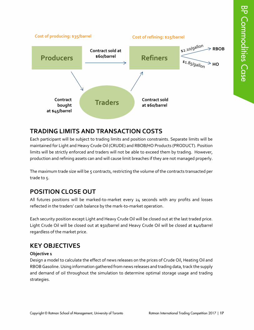
*All starting endowments of storage are free. Subsequent storage leased (due to overproduction) will be charged at a price of $500,000 per storage unit which can hold up to 10,000 barrels Industry-specific news will be released to participants based on their roles. Producers will receive expected production reports of their oil rigs (which are subject to changes throughout the simulation). Actual production may be different from the forecast, in which case producers will be informed of the quantity shock in the next expected production report. Producers will also be subject to shocks influencing the production price of crude and the time at which production is delivered. Refiners will receive information on the downstream RBOB Gasoline and Heating Oil markets which they must use to forecast future prices. Traders will receive “The International Tender Report” which describes the expected institutional orders activity. The interaction between different market participants, including their profit maximization objectives of each role and teamwork, is what will largely influence the overall profits of each team. Thus, participants have to optimize the dynamics of each role. The following is a simplified example of the case: Assume that RBOB and HO are currently trading at $2.10/gallon and $1.85/gallon respectively. Those outputs can be obtained using the Light Refinery, giving a Light Crude refined value of $2/gallon. If you convert this value into barrels: 42,000 * $2/gallon = $84,000 per 1,000 barrels, or $84/barrel. Refiners have bought ten contracts, agreeing to buy 5,000 barrels of Light Crude Oil from the producers and 5,000 barrels of Light Crude Oil from traders at a price of $60/barrel. In this scenario, refiners choose to operate only the Light Refinery. Traders initially bought Light Crude from producers at a spot price of $45/barrel. Profit generated by each member (per barrel):
• Producers: Price per contract - cost of producing oil per barrel = $60 - $35 = $25 • Refiners: Value of refined oil - cost of buying and refining oil = $84.00 - ($60 + $25) = -$1.00 • Traders: Price of contract sold - spot price of oil bought = $60 - $45 = $15
BP Com
modities C
ase
Copyright © Rotman School of Management, University of Toronto Rotman International Trading Competition 2017 | 17
TRADING LIMITS AND TRANSACTION COSTS Each participant will be subject to trading limits and position constraints. Separate limits will be maintained for Light and Heavy Crude Oil (CRUDE) and RBOB/HO Products (PRODUCT). Position limits will be strictly enforced and traders will not be able to exceed them by trading. However, production and refining assets can and will cause limit breaches if they are not managed properly. The maximum trade size will be 5 contracts, restricting the volume of the contracts transacted per trade to 5.
POSITION CLOSE OUT All futures positions will be marked-to-market every 24 seconds with any profits and losses reflected in the traders’ cash balance by the mark-to-market operation. Each security position except Light and Heavy Crude Oil will be closed out at the last traded price. Light Crude Oil will be closed out at $50/barrel and Heavy Crude Oil will be closed at $40/barrel regardless of the market price.
KEY OBJECTIVES Objective 1 Design a model to calculate the effect of news releases on the prices of Crude Oil, Heating Oil and RBOB Gasoline. Using information gathered from news releases and trading data, track the supply and demand of oil throughout the simulation to determine optimal storage usage and trading strategies.
Producers Refiners Contract sold at
$60/barrel
RBOB
Cost of producing: $35/barrel Cost of refining: $25/barrel
HO
Contract bought
at $45/barrel
Traders Contract sold at $60/barrel
BP Com
modities C
ase BP C
omm
odities Case

Copyright © Rotman School of Management, University of Toronto Rotman International Trading Competition 2017 | 18
Objective 2 Maximize profits as a team of producers, refiners, and traders by communicating and sharing private news information with each other. Note: Since this simulation requires a large number of participants in order to establish supply/demand, practice sessions for this case will be organized and held at specified times. After organized practice sessions are completed, cases will be run iteratively for model calibration purposes (“trading skillfully” cannot be practiced unless there are 20+ users online).
BP Com
modities C
ase

Copyright © Rotman School of Management, University of Toronto Rotman International Trading Competition 2017 | 19
S&P Global Credit Risk Case
OVERVIEW The S&P Global Credit Risk Case challenges participants to build and apply a credit risk model in a simulation where corporate bonds are traded. Participants will use both a Structural Model and the Altman Z-Score to predict potential changes to the companies’ credit ratings. Periodic news updates will require participants to make appropriate adjustments to the assumptions in their models and rebalance their portfolios accordingly. This case will test participants’ ability to develop a credit risk model, assess the impact of news releases on credit risk, and execute trading strategies accordingly to profit from mispricing opportunities.
DESCRIPTION In this case there will be 2 heats and teams will allocate 2 team members for each heat. Each participant may compete in only one of the 2 heats. A total of 4 team members will compete in the overall case. Each sub-heat will span 16 minutes, representing two calendar years. Each heat will involve 5 tradable securities. Trading from Excel using the Rotman API will be disabled. Real Time Data (RTD) links will be enabled.
Parameter Value
Number of trading sub-heats 4 Trading time per sub-heat 16 minutes (960 seconds)
Calendar time per sub-heat 2 calendar years
(4 weeks per month, 12 months in a year – total of 48 weeks in a year)
Compounding interval 1 week (10 seconds) Maximum order size 500 contracts
This case assumes that participants are working at a fixed income trading desk as a junior analyst. Participants are strongly encouraged to build a credit risk model according to the information
S&P G
lobal Credit Risk C
ase

Copyright © Rotman School of Management, University of Toronto Rotman International Trading Competition 2017 | 20
presented in the “Market Dynamics” section below. Two models will be introduced, the “Structural Model” and the “Altman Z-Score Model”. The Structural Model will be used to calculate the implied credit spreads for the bonds, while the Altman Z-Score Model can be used to determine the Z-Score and associated financial solvency category of the company. With the use of the two models, participants will be able to calculate the probabilities of a rating upgrade/downgrade and the fair prices of the corporate bonds. Then they will be able to implement a trading strategy and profit from mispricing opportunities. News items will be periodically released during the case, which may have an impact on the variables used in the two models. As these variables change, the implied credit spread and/or the Altman Z-Score may change, affecting the likelihood of a rating upgrade/downgrade. Participants will then have to adjust their trading strategies and portfolio positions. For more details about the variables used in the models and the news releases, please see the “Market Dynamics” and “News Releases” sections, respectively.
MARKET DYNAMICS There are five tradable zero-coupon corporate bonds that are issued by non-dividend paying public companies. All of these bonds have the same credit ratings at the beginning of the case. The characteristics of the bonds can be found in the table below.
BondA BondB BondC BondD BondE
Face Value (𝐷𝐷) 100 100 100 100 100
Coupon 0 0 0 0 0
Maturity (𝑇𝑇) 5 years from
now 5 years from
now 5 years from
now 5 years from
now 5 years from
now
Credit Rating A A A A A
Issuer Info Anaheim Manufacturing
BaseData Calyx Asset
Management Dayaria Milk
Products Ellen
Cosmetics
Volatility of Company’s Assets
(𝜎𝜎𝐴𝐴) 36% 35% 54% 35% 46%
Total Asset Value (in 100 millions)
(𝐴𝐴0) 100 185 130 80 140
Total Debt Value (in 100 millions)
60 110 35 50 55
Market Value of Equity
(in 100 millions) 40 75 95 30 85
S&P G
lobal Credit Risk C
ase

Copyright © Rotman School of Management, University of Toronto Rotman International Trading Competition 2017 | 21
Sales (in 100 millions)
100 160 35 60 60
EBIT (Earnings Before Interest
and Taxes) (in 100 millions)
20 60 10 40 35
Retained Earnings (in 100 millions)
15 30 5 10 25
Working Capital (in 100 millions)
40 20 10 10 20
There is an annual risk free rate (𝑡𝑡𝑓𝑓,𝑎𝑎) and a table provided by the credit rating agency with credit spreads (𝑠𝑠𝑟𝑟) that correspond to each rating. In equilibrium, bonds will be priced such that the implied yield to maturity (𝑤𝑤) is equal to 𝑡𝑡 + 𝑠𝑠𝑟𝑟 (risk free rate plus credit spread), where time to maturity will be expressed as the difference between the maturity (𝑇𝑇) and the current time (𝐸𝐸):
𝑃𝑃𝑡𝑡 =100
(1 + 𝑤𝑤)(𝑇𝑇−𝑡𝑡) =100
�1 + 𝑡𝑡𝑓𝑓,𝑎𝑎 + 𝑠𝑠𝑟𝑟�(𝑇𝑇−𝑡𝑡)
Rating Agency Credit Ratings
Rating Credit Spread (𝒔𝒔𝒓𝒓)
AAA 0.50% AA+ 1.00% AA 1.50% AA- 2.00% A+ 2.50% A 3.00% A- 3.50%
BBB+ 4.00% BBB 4.50% BBB- 5.00% BB+ 5.50% BB 6.00% BB- 6.50% B+ 7.00%
The credit rating agency will be releasing the updated credit ratings for each company on a quarterly basis. A company can be upgraded or downgraded by the credit rating agency only by one notch. For example, if a company has a current rating of A, its rating will be A+ in case of upgrade and A- in case of downgrade.
S&P G
lobal Credit Risk C
ase

Copyright © Rotman School of Management, University of Toronto Rotman International Trading Competition 2017 | 22
The senior fixed income fund managers understand that the change of the financial situation of a company will not be reflected immediately by these ratings since they are only updated quarterly. Therefore, they have suggested that you can also calculate an implied credit spread (𝑠𝑠𝑚𝑚) using real-time market data through a Structural Model, as explained in the following subsection. Structural Model The company’s liabilities are composed of two parts: equity and debt. We assume that the equity does not receive dividends and that the debt is in the form of a zero coupon bond with face value (𝐷𝐷) and maturity (𝑇𝑇). If at maturity (t = 𝑇𝑇), the value of the assets, 𝐴𝐴𝑇𝑇, is greater than the value of the debt, the company will pay its debt. If instead, the value of the assets at maturity is smaller than the value of the debt, the company will go bankrupt. If this occurs, the bondholders will receive the value of the asset and the shareholders will receive nothing. Conceptually, this means that the equity portion of a company can be modelled as a European call option written on the value of the assets (𝐴𝐴𝑡𝑡) with a strike price equal to the face value of the debt (𝐷𝐷). Therefore, Black-Scholes can be used to model the value of the equity, leading to the following model1 for the implied credit spread. Let 𝐿𝐿𝑡𝑡, the measure for the company’s leverage at time 𝐸𝐸, be defined by the following formula:
𝐿𝐿𝑡𝑡 =𝐸𝐸𝑡𝑡𝑡𝑡𝑡𝑡𝐸𝐸𝑎𝑎𝐸𝐸 𝑣𝑣𝑡𝑡𝑤𝑤𝑡𝑡𝐸𝐸 𝑜𝑜𝑜𝑜 𝐸𝐸𝐸𝐸𝑑𝑑𝐸𝐸𝐸𝐸𝑡𝑡𝑡𝑡𝑡𝑡𝐸𝐸𝑎𝑎𝐸𝐸 𝑣𝑣𝑡𝑡𝑤𝑤𝑡𝑡𝐸𝐸 𝑜𝑜𝑜𝑜 𝑡𝑡𝑠𝑠𝑠𝑠𝐸𝐸𝐸𝐸𝑠𝑠
=𝐷𝐷 𝐸𝐸−𝑟𝑟(𝑇𝑇−𝑡𝑡)
𝐴𝐴𝑡𝑡
Where, 𝐷𝐷 is the face value of debt; 𝑡𝑡 is the risk free rate; 𝑇𝑇 − 𝐸𝐸 is the time to maturity of the zero-coupon bond in years; 𝐴𝐴𝑡𝑡 is the current value of assets at the present time 𝐸𝐸. The implied credit spread is then calculated as:
𝑠𝑠𝑚𝑚 = −𝑤𝑤𝑎𝑎 �𝑁𝑁(𝐸𝐸2) + 𝑁𝑁(−𝐸𝐸1)
𝐿𝐿𝑡𝑡�
(𝑇𝑇 − 𝐸𝐸)
Where,
𝐸𝐸1 =− 𝑤𝑤𝑎𝑎(𝐿𝐿𝑡𝑡)𝜎𝜎𝐴𝐴�(𝑇𝑇 − 𝐸𝐸)
+12𝜎𝜎𝐴𝐴�(𝑇𝑇 − 𝐸𝐸)
𝐸𝐸2 = 𝐸𝐸1 − 𝜎𝜎𝐴𝐴�(𝑇𝑇 − 𝐸𝐸). 𝑇𝑇 − 𝐸𝐸 is the time to maturity of the zero-coupon bond in years; 𝜎𝜎𝐴𝐴 is the volatility of the company’s assets; 𝑁𝑁(𝐸𝐸) is the standard normal cumulative distribution function of 𝐸𝐸.
1 This model is known in the l iterature as the Merton Model.
S&P G
lobal Credit Risk C
ase S&
P Global C
redit Risk Case

Copyright © Rotman School of Management, University of Toronto Rotman International Trading Competition 2017 | 23
For further details, including a formal derivation of this Structural Model, please see the Appendix. Altman Z-Score Model The fund managers suggest that you also consider the Altman Z-Score to estimate the default probability of the companies. The Altman Z-Score is calculated as follows:
𝑍𝑍 = 1.2𝑋𝑋1 + 1.4𝑋𝑋2 + 3.3𝑋𝑋3 + 0.6𝑋𝑋4 + 0.99𝑋𝑋5
𝑋𝑋1 is Working Capital/Total Assets 𝑋𝑋2 is Retained Earnings/Total Assets
𝑋𝑋3 is EBIT/Total assets 𝑋𝑋4 is Market Value of Equity/Total Debt
𝑋𝑋5 is Sales/Total Debt Based on the Z-Score, the company can be classified into one of three different categories: If 𝑍𝑍 > 2.99, there is a low probability of bankruptcy (“Safe” Zone). If 1.81 < 𝑍𝑍 ≤ 2.99, there is a moderate probability of bankruptcy (“Grey” Zone). If 𝑍𝑍 ≤ 1.81, there is a high probability of bankruptcy (“Distress” Zone). Evaluating the Probability of Credit Rating Downgrade/Upgrade Your senior analysts have come up with the following table, which predicts the probability of a rating upgrade/downgrade. The rows of the table are based on the difference between the Structural Model implied credit spread (𝑠𝑠𝑚𝑚) and the credit spread associated with the current credit rating (𝑠𝑠𝑟𝑟), while the columns are based on the categories found using the Altman Z-Score Model.
Probability of Downgrade Probability of Upgrade
Difference (𝒔𝒔𝒎𝒎 − 𝒔𝒔𝒓𝒓)
Safe Grey Distressed Safe Grey Distressed
𝑠𝑠𝑚𝑚 − 𝑠𝑠𝑟𝑟 < −2% 0.0% 0.0% 0.0% 75.0% 65.0% 55.0%
−2.0% ≤ 𝑠𝑠𝑚𝑚 − 𝑠𝑠𝑟𝑟 < −1.5% 0.0% 0.0% 0.0% 65.0% 55.0% 45.0%
−1.5% ≤ 𝑠𝑠𝑚𝑚 − 𝑠𝑠𝑟𝑟 < −1.0% 0.0% 0.0% 0.0% 55.0% 45.0% 35.0%
−1.0% ≤ 𝑠𝑠𝑚𝑚 − 𝑠𝑠𝑟𝑟 < −0.5% 0.0% 0.0% 0.0% 45.0% 35.0% 25.0%
−0.5% ≤ 𝑠𝑠𝑚𝑚 − 𝑠𝑠𝑟𝑟 < 0.0% 25.0% 35.0% 45.0% 40.0% 30.0% 20.0%
0.0% ≤ 𝑠𝑠𝑚𝑚 − 𝑠𝑠𝑟𝑟 < 0.5% 35.0% 45.0% 55.0% 35.0% 25.0% 15.0%
0.5% ≤ 𝑠𝑠𝑚𝑚 − 𝑠𝑠𝑟𝑟 < 1.0% 45.0% 55.0% 65.0% 0.0% 0.0% 0.0%
1.0% ≤ 𝑠𝑠𝑚𝑚 − 𝑠𝑠𝑟𝑟 < 1.5% 55.0% 65.0% 75.0% 0.0% 0.0% 0.0%
1.5% ≤ 𝑠𝑠𝑚𝑚 − 𝑠𝑠𝑟𝑟 < 2.0% 65.0% 75.0% 85.0% 0.0% 0.0% 0.0%
𝑠𝑠𝑚𝑚 − 𝑠𝑠𝑟𝑟 ≥ 2.0% 75.0% 85.0% 95.0% 0.0% 0.0% 0.0%
S&P G
lobal Credit Risk C
ase

Copyright © Rotman School of Management, University of Toronto Rotman International Trading Competition 2017 | 24
These probabilities should be used to find the expected credit spread as shown in the formula below:
𝐸𝐸(𝑠𝑠) = 𝐸𝐸𝑢𝑢 ∙ 𝑠𝑠𝑟𝑟𝑢𝑢 + 𝐸𝐸𝑑𝑑 ∙ 𝑠𝑠𝑟𝑟𝑑𝑑 + (1 − 𝐸𝐸𝑢𝑢 − 𝐸𝐸𝑑𝑑) ∙ 𝑠𝑠𝑟𝑟 Where, 𝐸𝐸𝑢𝑢 and 𝐸𝐸𝑑𝑑 are, respectively, the probabilities of a rating upgrade or downgrade; 𝑠𝑠𝑟𝑟𝑢𝑢 is the credit spread in the case of upgrade according to the rating agency’s table of credit ratings; 𝑠𝑠𝑟𝑟𝑑𝑑 is the credit spread in case of downgrade according to the rating agency’s table of credit ratings; 𝑠𝑠𝑟𝑟 is the current credit spread according to the rating agency’s table of credit ratings. This expected credit spread should then be used to calculate the fair value for the zero-coupon bond. Traders are expected to compare this fair value to the market value and make appropriate trading decisions. Below is an example of how participants should price a bond with a company rating of A, two years left to maturity, and a risk free rate of 2% annualized (compounded weekly). Input:
• Company Rating = A • Expected credit spread 𝐸𝐸(𝑠𝑠) = 4.00% • Time to Maturity (𝑇𝑇 − 𝐸𝐸) = 2 𝑤𝑤𝐸𝐸𝑡𝑡𝑡𝑡𝑠𝑠 • Risk free rate annualized weekly compounded 𝑡𝑡𝑓𝑓,𝑤𝑤 = 2%
The equivalent annual rate 𝑡𝑡𝑎𝑎 is
𝑡𝑡𝑓𝑓,𝑎𝑎 = �1 +𝑡𝑡𝑤𝑤𝑎𝑎�𝑛𝑛
= �1 +2%48
�48≈ 2.0197%
Where 𝑎𝑎 is the number of weeks in a year. As stated above, we assume that there are 48 weeks in a year. The price of the bond (𝑃𝑃𝑡𝑡) is therefore:
𝑃𝑃𝑡𝑡 =100
�1 + 𝑡𝑡𝑓𝑓,𝑎𝑎 + 𝐸𝐸(𝑠𝑠)�𝑇𝑇−𝑡𝑡 =
100(1 + 2.0197% + 4.00%)2 ≈ 88.97
S&P G
lobal Credit Risk C
ase

Copyright © Rotman School of Management, University of Toronto Rotman International Trading Competition 2017 | 25
NEWS RELEASE News items will be released every quarter. They will affect the variables within the Structural Model and the Altman Z-Score Model. Participants should be able to identify relevant news, assess their impact, and execute appropriate trading strategies. The following is a simple example of the type of information that will appear in the news item, and how to interpret in relationship to the above valuation model. Please note that news in the case may include more information than the following examples, and traders should read all news carefully for relevant information:
“Calyx Asset Management takes on an additional $200 million of debt financing for their share repurchase program”
This will increase the level of total debt of Calyx Asset Management by $200 million, which will directly increase the company’s leverage, (𝐿𝐿𝑡𝑡). This in turn increases the implied credit spread (𝑠𝑠𝑚𝑚) in the Structural Model through the variables 𝐸𝐸1 and 𝐸𝐸2. One can then compare this new implied credit spread (𝑠𝑠𝑚𝑚) with the credit spread given by the credit rating agency (𝑠𝑠𝑟𝑟). For example, if the initial difference between the two credit spreads (𝑠𝑠𝑚𝑚 − 𝑠𝑠𝑟𝑟) was 0.40%, the impact of the news may move the difference to 0.90%. Looking at the upgrade/downgrade table, if the company is in the “Safe” zone, the probability of downgrade will increase from 35% to 45% and the probability of upgrade will decrease from 35% to 0%. Note that the increase in total debt associated with this news will also affect the Altman Z-Score Model through variables 𝑋𝑋4 (Market Value of Equity/Total Debt) and 𝑋𝑋5 (Sales/Total Debt). A detailed explanation of a news release on the Altman Z-Score Model is given below. A sample news release impacting the Altman Z-Score Model is:
“Major weather conditions reduce demand for Anaheim Manufacturing’s products, decreasing the company’s revenue by $500M”
In this case, the news item decreases the sales of Anaheim Manufacturing by $500M, which decreases 𝑋𝑋5 (Sales/Total Debt) in the Altman Z-Score Model. Hence, the Altman Z-Score decreases for Anaheim Manufacturing, which in turn could move the state of the company’s financial solvency from either the “Safe” zone to the “Grey” zone or from the “Grey” zone to the “Distress” Zone. For example, assume that Anaheim Manufacturing is initially in “Safe” zone with a difference between 𝑠𝑠𝑚𝑚 and 𝑠𝑠𝑟𝑟 of 0.00%. If the news release changes the Altman Z-Score Model for Anaheim Manufacturing so that the company moves from “Safe” zone to “Grey” zone, then the probability of downgrade changes from 35% to 45% and the probability of upgrade changes from 35% to 25%.
S&P G
lobal Credit Risk C
ase

Copyright © Rotman School of Management, University of Toronto Rotman International Trading Competition 2017 | 26
TRADING LIMITS AND TRANSACTION COSTS Each participant will be subject to gross and net trading limits. The gross trading limit reflects the sum of the absolute values of the long and short positions across all securities; while the net trading limit reflects the sum of long and short positions such that short positions negate any long positions. Trading limits will be strictly enforced and participants will not be able to exceed them. The maximum order size will be 500 bonds, and transaction fees will be set to 2 cents per bond.
POSITION CLOSE-OUT Any open position will be closed out at the end of each sub-heat based on the price of the bond using the credit spread provided by the credit rating agency. This includes any long or short position open in any security.
KEY OBJECTIVES Objective 1 Build a credit risk model that incorporates both the Structural Model and the Altman Z-Score Model which can be used in conjunction with the ratings issues by the credit agency to find the expected credit spread and fair value for the zero-coupon bonds. By understanding the variables that drive the credit risk models, participants should be able to identify and exploit mispricing opportunities to generate profits. Objective 2 Analyze the impact of news releases on the relevant variables of the model. News items will affect one or more parameters in the Structural Model and/or the Altman Z-Score Model, and consequently the probability of a credit rating change. Traders should update their credit risk models to reflect these changes and rebalance their portfolios accordingly. Objective 3 Manage exposure to market risk. To minimize their bond portfolios’ exposure to market risk, participants are encouraged to take positions in more than one bond to reduce losses associated with idiosyncratic risks of each bond.
S&P G
lobal Credit Risk C
ase

Copyright © Rotman School of Management, University of Toronto Rotman International Trading Competition 2017 | 27
APPENDIX
The company’s liabilities are composed of the following two parts: equity and debt. The equity does not receive dividends and the debt is in the form of a zero coupon bond with face value equal to 𝐷𝐷 and maturity at time 𝑇𝑇. If at maturity (𝑇𝑇), the value of the of the assets, 𝐴𝐴𝑇𝑇 , is greater than the value of the debt, the company will pay its debt. If at maturity (𝑇𝑇), the value of the of the assets, 𝐴𝐴𝑇𝑇, is smaller than the value of the debt, the company will go bankrupt. Bondholders will receive the value of the assets and the shareholders will not receive anything. The company cannot go bankrupt before time 𝑇𝑇. Formalizing this description: the value of the assets is assumed to follow a geometric Brownian motion described by the following equation:
𝐸𝐸𝐴𝐴 = 𝜇𝜇𝐴𝐴 𝐴𝐴 𝐸𝐸𝐸𝐸 + 𝜎𝜎𝐴𝐴 𝐴𝐴 𝐸𝐸𝑑𝑑 Where, 𝜇𝜇𝐴𝐴 is the drift of the asset value - assumed to be equal to zero in this case; 𝜎𝜎𝐴𝐴 is the volatility of the company’s assets; 𝐸𝐸𝑑𝑑 is a standard Wiener process. The value of the assets at time 𝐸𝐸 is then equal to
𝐴𝐴𝑡𝑡 = 𝐴𝐴0𝐸𝐸𝐸𝐸𝐸𝐸 ��𝜇𝜇𝐴𝐴 −𝜎𝜎𝐴𝐴2
2 � 𝐸𝐸 + 𝜎𝜎𝐴𝐴2 √𝐸𝐸 𝑑𝑑𝑡𝑡�
where 𝑑𝑑𝑡𝑡~ 𝑁𝑁(0, 𝐸𝐸). The expectation of 𝐴𝐴𝑡𝑡 is:
𝐸𝐸(𝐴𝐴𝑡𝑡) = 𝐴𝐴0𝐸𝐸𝐸𝐸𝐸𝐸 (𝜇𝜇𝐴𝐴𝐸𝐸) At time 𝑇𝑇, the value of the equity will be:
𝐸𝐸𝑇𝑇 = 𝑡𝑡𝑡𝑡𝐸𝐸[𝐴𝐴𝑇𝑇 − 𝐷𝐷, 0] The above shows that the value of the equity looks like the payoff of a (European) call option written on the value of the assets (𝐴𝐴) with a strike price equal to the face value of the debt (𝐷𝐷). Using Black-Scholes:
𝐸𝐸0 = 𝐴𝐴0𝑁𝑁(𝐸𝐸1) − 𝐷𝐷𝐸𝐸−𝑟𝑟𝑇𝑇𝑁𝑁(𝐸𝐸2)
S&P G
lobal Credit Risk C
ase

Copyright © Rotman School of Management, University of Toronto Rotman International Trading Competition 2017 | 28
with
𝐸𝐸1 =𝑤𝑤𝑎𝑎 �𝐴𝐴0𝐸𝐸
𝑟𝑟(𝑇𝑇−𝑡𝑡)
𝐷𝐷 �
𝜎𝜎𝐴𝐴�(𝑇𝑇 − 𝐸𝐸)+
12𝜎𝜎𝐴𝐴�(𝑇𝑇 − 𝐸𝐸)
𝐸𝐸2 = 𝐸𝐸1 − 𝜎𝜎𝐴𝐴�(𝑇𝑇 − 𝐸𝐸) where 𝑡𝑡 is the risk-free rate. Let 𝐿𝐿𝑡𝑡 be a measure of the leverage used by the company and defined as:
𝐿𝐿𝑡𝑡 =𝐸𝐸𝑡𝑡𝑡𝑡𝑡𝑡𝐸𝐸𝑎𝑎𝐸𝐸 𝑣𝑣𝑡𝑡𝑤𝑤𝑡𝑡𝐸𝐸 𝑜𝑜𝑜𝑜 𝐸𝐸𝐸𝐸𝑑𝑑𝐸𝐸𝐸𝐸𝑡𝑡𝑡𝑡𝑡𝑡𝐸𝐸𝑎𝑎𝐸𝐸 𝑣𝑣𝑡𝑡𝑤𝑤𝑡𝑡𝐸𝐸 𝑜𝑜𝑜𝑜 𝑡𝑡𝑠𝑠𝑠𝑠𝐸𝐸𝐸𝐸𝑠𝑠
=𝐷𝐷 𝐸𝐸−𝑟𝑟(𝑇𝑇−𝑡𝑡)
𝐴𝐴𝑡𝑡
Then we can write the current value of the Equity as:
𝐸𝐸t = 𝐴𝐴t[𝑁𝑁(𝐸𝐸1)− 𝐿𝐿𝑡𝑡 𝑁𝑁(𝐸𝐸2)] where,
𝐸𝐸1 =− 𝑤𝑤𝑎𝑎(𝐿𝐿𝑡𝑡)𝜎𝜎𝐴𝐴�(𝑇𝑇 − 𝐸𝐸)
+12𝜎𝜎𝐴𝐴�(𝑇𝑇 − 𝐸𝐸)
𝐸𝐸2 = 𝐸𝐸1 − 𝜎𝜎𝐴𝐴�(𝑇𝑇 − 𝐸𝐸). The current value of the debt (at time 𝐸𝐸) is equal to:
𝐵𝐵t = 𝐴𝐴t − 𝐸𝐸t Substituting for 𝐸𝐸t from above:
𝐵𝐵t = 𝐴𝐴t[𝑁𝑁(−𝐸𝐸1) + 𝐿𝐿 𝑁𝑁(𝐸𝐸2)] Note that the current value of debt 𝐵𝐵0 can also be expressed by discounting the face value at the implied yield to maturity (𝑤𝑤):
𝐵𝐵t = 𝐷𝐷𝐸𝐸−𝑦𝑦(𝑇𝑇−𝑡𝑡) = 𝐷𝐷−𝑟𝑟(𝑇𝑇−𝑡𝑡)𝐸𝐸(𝑟𝑟−𝑦𝑦)(𝑇𝑇−𝑡𝑡) = 𝐴𝐴t𝐿𝐿𝑡𝑡𝐸𝐸(𝑟𝑟−𝑦𝑦)(𝑇𝑇−𝑡𝑡) It follows that:
𝐴𝐴t𝐿𝐿𝑡𝑡𝐸𝐸(𝑟𝑟−𝑦𝑦)(𝑇𝑇−𝑡𝑡) = 𝐴𝐴t[𝑁𝑁(−𝐸𝐸1) + 𝐿𝐿𝑡𝑡𝑁𝑁(𝐸𝐸2)]
S&P G
lobal Credit Risk C
ase

Copyright © Rotman School of Management, University of Toronto Rotman International Trading Competition 2017 | 29
Therefore, the implied yield to maturity (𝑤𝑤) can be calculated as:
𝑤𝑤 = 𝑡𝑡 −𝑤𝑤𝑎𝑎 �𝑁𝑁(𝐸𝐸2) + 𝑁𝑁(−𝐸𝐸1)
𝐿𝐿𝑡𝑡�
(𝑇𝑇 − 𝐸𝐸)
And the implied credit spread (𝑠𝑠𝑚𝑚) is calculated as:
𝑠𝑠𝑚𝑚 = 𝑤𝑤 − 𝑡𝑡 = −𝑤𝑤𝑎𝑎 �𝑁𝑁(𝐸𝐸2) + 𝑁𝑁(−𝐸𝐸1)
𝐿𝐿𝑡𝑡�
(𝑇𝑇 − 𝐸𝐸)
S&P G
lobal Credit Risk C
ase

Copyright © Rotman School of Management, University of Toronto Rotman International Trading Competition 2017 | 30
Quantitative Outcry Case
OVERVIEW The Quantitative Outcry case challenges participants to apply their understanding of macroeconomics to determine the effect of news releases on the world economy as captured by the Rotman Index (RT100). The RT100 Index is a composite index reflective of global political, economic, and market conditions. Participants will be required to interpret and react to both quantitative and qualitative news releases in trading futures written on the RT100 Index based on their analysis of the news’ impact on the index.
DESCRIPTION There will be 2 heats with 4 team members competing for the entire heat. The 4 team members will comprise of 2 analysts and 2 traders who will rotate positions for the second heat. Team members acting as traders in the first heat must act as analysts in the second heat and vice versa. Each heat will last 30 minutes and represent six months of calendar time. Traders will be trading futures contracts on the RT100 Index.
Parameter Value Number of trading heats 2
Trading time per heat 30 minutes Calendar time per heat 6 months (2 quarters)
The Fleck Atrium in the Rotman Building will serve as the trading pit for the traders, while the analysts will share a desktop in the Rotman Finance Lab. Analysts will have access to detailed news releases, while traders in the pit will only have access to news headlines. It will be the role of the analyst to quantify the impact of news releases on the RT100 Index while traders will be required to react and trade according to the analysts’ instructions. As analysts and traders will be on separate floors, it is essential for teams to develop non-verbal communication strategies. Electronic devices are not permitted during this case.
MARKET DYNAMICS The value of the RT100 Index is determined by the quarterly GDP growth, in billions, of the following 6 economies: Canada, the United States, Brazil, Japan, Germany and South Africa. Each country’s GDP contributes to a percentage of the RT100 Index. The initial level of RT100 is 1,000 at t=0. The RT100 Index is quoted in units and the futures contracts are written on the RT100 Index. The contract multiplier for RT100 futures is $10.
Quantitative O
utcry Case

Copyright © Rotman School of Management, University of Toronto Rotman International Trading Competition 2017 | 31
Therefore, 1 futures contract is worth $10*RT100 Index. If the RT100 Index is at 995 and a trader owns 1 future contract, his/her position will be worth $9,950 (= $10*995). Economic statistics for each of the countries are collected and released throughout the trading session, and will determine the exact trading level of the RT100 Index at the midpoint and at the end of the trading period (15 minutes and 30 minutes of the simulation equivalent to 3 months and 6 months in real calendar time). There is no exchange rate risk (all values are expressed in the same currency). The value of the RT100 Index at t=15 minutes is calculated by the following formula:
𝑅𝑅𝑇𝑇100𝑉𝑉𝑎𝑎𝑉𝑉𝑢𝑢𝑉𝑉 𝑎𝑎𝑡𝑡 𝑡𝑡=15 = 1000 + 𝐶𝐶𝑡𝑡𝑎𝑎𝑡𝑡𝐸𝐸𝑡𝑡(𝐴𝐴𝐴𝐴𝑡𝑡𝑢𝑢𝑎𝑎𝑉𝑉 𝑄𝑄1 𝐺𝐺𝐺𝐺𝐺𝐺−𝐺𝐺𝑟𝑟𝑉𝑉𝑃𝑃𝑃𝑃𝑃𝑃𝑢𝑢𝑃𝑃 𝑄𝑄1 𝐺𝐺𝐺𝐺𝐺𝐺) + 𝑈𝑈𝑈𝑈𝐴𝐴(𝐴𝐴𝐴𝐴𝑡𝑡𝑢𝑢𝑎𝑎𝑉𝑉 𝑄𝑄1 𝐺𝐺𝐺𝐺𝐺𝐺−𝐺𝐺𝑟𝑟𝑉𝑉𝑃𝑃𝑃𝑃𝑃𝑃𝑢𝑢𝑃𝑃 𝑄𝑄1 𝐺𝐺𝐺𝐺𝐺𝐺) …+ 𝑈𝑈𝑜𝑜𝑡𝑡𝐸𝐸ℎ 𝐴𝐴𝑜𝑜𝑡𝑡𝑅𝑅𝐸𝐸𝑡𝑡(𝐴𝐴𝐴𝐴𝑡𝑡𝑢𝑢𝑎𝑎𝑉𝑉 𝑄𝑄1 𝐺𝐺𝐺𝐺𝐺𝐺−𝐺𝐺𝑟𝑟𝑉𝑉𝑃𝑃𝑃𝑃𝑃𝑃𝑢𝑢𝑃𝑃 𝑄𝑄1 𝐺𝐺𝐺𝐺𝐺𝐺)
In other words, every $1 billion of actual year-over-year GDP increase will cause a 1 point increase in the RT100 Index. Consequently, every $1 billion of actual GDP shortfall will cause a 1 point decrease in the RT100 Index. The quarterly GDP for each country is comprised of aggregate production in three independent sectors: Manufactured Goods, Services, and Raw Materials. At the beginning of the outcry case, estimates for the aggregate quarterly GDP of each country and sector will be released. Throughout the quarter, news releases will provide estimates and information that will allow analysts to construct expectations for each country and each sector. The following is a sample series of data for Q1 Canada:
• Canadian Q1 GDP last year was $100 billion. This year in Q1, the market expects manufactured goods of $30 billion, services of $60 billion, and raw materials of $10 billion.
• General workers protest hits Canada manufacturing sector, causing minor production delays.
• Strong global commodities prices lift raw materials output across the globe by as much as 10%.
• New policies cause $7 billion increase in services spending. • RELEASE – Canadian Manufacturing for Q1: $28 billion • RELEASE – Canadian Services for Q1: $67 billion • RELEASE – Canadian Raw Materials for Q1: $11 billion
The sum of the independent sectors, and thus the resulting Q1 Canadian GDP, is $106 billion. This is $6 billion above last year’s Q1 GDP of $100 billion and would cause the RT100 Index to increase by 6 points. This, in addition to the effects of the other 5 countries, will determine the RT100 Index at the 15-minute mark (and then the 30-minute mark).
Quantitative O
utcry Case

Copyright © Rotman School of Management, University of Toronto Rotman International Trading Competition 2017 | 32
TRADERS’ ROLES Traders are responsible to interpret the signals from the analysts located in the Rotman Finance Lab and trade the RT100 index. Traders will have to find other teams who are willing to act as counterparties to complete their trades. Traders are also responsible for keeping track of their position and communicating it to analysts.
ANALYSTS’ ROLES Analysts are responsible for interpreting the detailed news they receive on the RIT and communicate their findings to the traders in the Fleck Atrium. Analysts are also responsible for submitting analyst estimate forms (refer to the Cash Bonuses section for more details) and making spot trades. Spot Trades In addition to the transactions executed by the traders in the Fleck Atrium, analysts in the Rotman Finance Lab are allowed to make up to 2 spot trades per heat, with a maximum of 50 contracts in each trade. The spot trades will be executed at the current spot price of the RT100 Index posted on the screen. The spot contract has a contract multiplier of $10. Therefore, if an analyst owns 1 spot contract when the RT100 Index is at 1,023, his/her position will be worth $10,230 (= $10*1,023). The spot trades allow each team to have an opportunity to close out their positions in a timely manner. Moreover, since the futures market will be driven by trader activity, while the spot market is based on the actual economic indicators realized, there may be arbitrage profit opportunities due to inefficiencies in the two markets (the actual market and the spot market). These trades are added to the aggregate futures position of the team. The soft and hard trading restriction limits discussed below also apply to trades made by analysts in the Rotman Finance Lab.
CASH BONUSES AND TRADING P&L Analyst Estimates Throughout the trading heat, analysts will be required to submit a point estimate of where they believe the RT100 Index will settle at the 15 and 30 minute marks. These estimates are due by the 10 and 25 minute marks, respectively (i.e. 5 minutes before the end of the quarter). These time limits will be tracked solely based on the trading software. Participants should refrain from using external devices (online timers, cell phones, watches, etc.) to track the time limits. Analysts will be graded based on their prediction accuracy and bonus cash will be allocated to the teams with the most accurate estimate. Counterparties At the end of trading, all submitted tickets will be reviewed and each team will be given a counterparty score based on the number of different trading counterparties they transacted with
Quantitative O
utcry Case

Copyright © Rotman School of Management, University of Toronto Rotman International Trading Competition 2017 | 33
throughout the trading session. Teams will be awarded bonus cash based on the number of different counterparties with which they transacted. Bonus Cash Calculations Each team will be ranked based on its performance and split into quintiles for each of the 2 bonus calculations. The top quintile for each bonus pool will be assigned a 5% bonus, the second 4%, and so on until the last quintile, which is assigned a 1% bonus. The 2 last placed teams are assigned a 0% bonus. Bonuses are never negative, and they are applied at the end of the heat based on the team’s absolute performance throughout the heat. Trading P&L Trading P&L will be calculated in a similar fashion as the social outcry case (with the addition of trading fines as described below). Trading P&L will then be modified by all bonuses (Analyst Estimates and Counterparties). The following is an example of a P&L calculation:
• Bought 5 RT100 Index futures at 1,000 • Sold 5 RT100 Index spot contracts at 1,100
The team is ranked at the top quintile for the bonus pool of Analyst Estimates and the third quintile for Counterparties
𝑃𝑃𝑡𝑡𝑜𝑜𝑜𝑜𝑅𝑅𝐸𝐸 𝐵𝐵𝐸𝐸𝑜𝑜𝑜𝑜𝑡𝑡𝐸𝐸 𝐵𝐵𝑜𝑜𝑎𝑎𝑡𝑡𝑠𝑠𝐸𝐸𝑠𝑠 = (1,100− 1,000) × $10 × 5 − $12 × 10 = $4,990
𝐵𝐵𝑜𝑜𝑎𝑎𝑡𝑡𝑠𝑠𝐸𝐸𝑠𝑠 = |$4,990| × 5% + |$4,990| × 3% = $399.20
𝑇𝑇𝑜𝑜𝐸𝐸𝑡𝑡𝑤𝑤 𝑃𝑃&𝐿𝐿 = $4,990.00 + $399.20 = $5,389.20
The following is an example when a trader has a negative P&L:
• Bought 5 RT100 Index futures at 1,000 • Sold 5 RT100 Index spot contracts at 900 • The team is ranked at the top quintile for the bonus pool of Analyst Estimates and the third
quintile for Counterparties 𝑃𝑃𝑡𝑡𝑜𝑜𝑜𝑜𝑅𝑅𝐸𝐸 𝐵𝐵𝐸𝐸𝑜𝑜𝑜𝑜𝑡𝑡𝐸𝐸 𝐵𝐵𝑜𝑜𝑎𝑎𝑡𝑡𝑠𝑠𝐸𝐸𝑠𝑠 = (900− 1000) × $10 × 5 − $1 × 10
= −$5,010 𝐵𝐵𝑜𝑜𝑎𝑎𝑡𝑡𝑠𝑠𝐸𝐸𝑠𝑠 = |$5,010| × 5% + |−$5,010| × 3%
= $400.80 𝑇𝑇𝑜𝑜𝐸𝐸𝑡𝑡𝑤𝑤 𝑃𝑃&𝐿𝐿 = −$5,010.00 + $400.80
= $4,609.20
2 Brokerage commission of $1 per contract traded – explained in Trading Limits and Transaction Costs – there have been 10 contracts traded in this example, 5 to buy and 5 to sell.
Quantitative O
utcry Case

Copyright © Rotman School of Management, University of Toronto Rotman International Trading Competition 2017 | 34
TRADING LIMITS AND TRANSACTION COSTS Each team has a starting position of 0 contracts, a soft trading limit of 200 contracts, and a fixed hard trading limit of 500 contracts on their net positions. On a best-efforts basis, each team will be notified as it approaches its soft and hard limits. If a team exceeds its soft limit, it will be charged a fine proportional to how much they exceed the soft limit. The amount by which a team exceeds the initial soft limit of 200 will become their new soft limit. The fine per contract above the soft limit is $50. For instance, if Team A’s net position is at 220, they will be charged a fine of $50*20 = $1,000 (they have exceeded their soft limit of 200 by 20 contracts). For Team A, 220 is now the new soft limit. As long as Team A’s position remains below 220, there will be no additional fines. If Team A bought more and had a new net position of 280, then they would be charged an additional fine of $50*60 = $3,000 which is the difference between the new net position and new soft limit. If a team does not exceed its soft limit, it will not be charged any fines. Any team that exceeds the hard limit of 500 will be automatically disqualified from the outcry. They will be given a rank equal to that of last place for that sub-heat. In addition, there is a zero tolerance policy with regards to electronic communication. Any trader or analyst seen by an RITC staff member using or holding a cell phone or any other electronic device during the trading heats will be immediately disqualified. RITC staff will be positioned throughout the pit and the trading lab to monitor this. Each transaction on futures has a maximum volume of 20 contracts per trade. Once more, analysts in the Rotman Finance Lab are allowed to make up to 2 spot trades during each heat, with up to 50 contracts in each trade. Each contract will be charged a brokerage commission of $1 per contract.
POSITION CLOSE-OUT Each team’s position will be settled at the end of the trading session by closing out their remaining positions at the final spot price.
KEY OBJECTIVES Objective 1 Traders can generate profits by interpreting news headlines and going long on positive news and short on negative news. Traders are also encouraged to trade with as many different counterparties to capitalize on the bonus structure.
Quantitative O
utcry Case
Quantitative O
utcry Case

Copyright © Rotman School of Management, University of Toronto Rotman International Trading Competition 2017 | 35
Objective 2 Analysts should track news releases and attempt to accurately estimate the value of the RT100 Index in order to develop a profitable trading strategy and communicate it efficiently to the traders. Additionally, the analyst should submit their index estimates in a timely manner and develop effective communication methods with the traders to quickly communicate trading strategies.
Quantitative O
utcry Case
Copyright © Rotman School of Management, University of Toronto Rotman International Trading Competition 2017 | 36
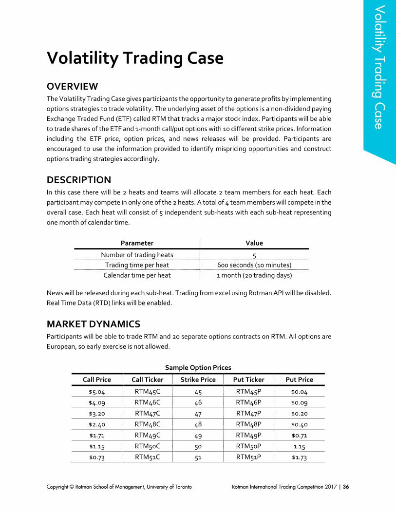
Volatility Trading Case OVERVIEW The Volatility Trading Case gives participants the opportunity to generate profits by implementing options strategies to trade volatility. The underlying asset of the options is a non-dividend paying Exchange Traded Fund (ETF) called RTM that tracks a major stock index. Participants will be able to trade shares of the ETF and 1-month call/put options with 10 different strike prices. Information including the ETF price, option prices, and news releases will be provided. Participants are encouraged to use the information provided to identify mispricing opportunities and construct options trading strategies accordingly.
DESCRIPTION In this case there will be 2 heats and teams will allocate 2 team members for each heat. Each participant may compete in only one of the 2 heats. A total of 4 team members will compete in the overall case. Each heat will consist of 5 independent sub-heats with each sub-heat representing one month of calendar time.
Parameter Value
Number of trading heats 5 Trading time per heat 600 seconds (10 minutes)
Calendar time per heat 1 month (20 trading days) News will be released during each sub-heat. Trading from excel using Rotman API will be disabled. Real Time Data (RTD) links will be enabled.
MARKET DYNAMICS Participants will be able to trade RTM and 20 separate options contracts on RTM. All options are European, so early exercise is not allowed.
Sample Option Prices
Call Price Call Ticker Strike Price Put Ticker Put Price
$5.04 RTM45C 45 RTM45P $0.04
$4.09 RTM46C 46 RTM46P $0.09
$3.20 RTM47C 47 RTM47P $0.20
$2.40 RTM48C 48 RTM48P $0.40
$1.71 RTM49C 49 RTM49P $0.71
$1.15 RTM50C 50 RTM50P 1.15
$0.73 RTM51C 51 RTM51P $1.73
Volatility Trading C
ase

Copyright © Rotman School of Management, University of Toronto Rotman International Trading Competition 2017 | 37
$0.44 RTM52C 52 RTM52P $2.44
$0.24 RTM53C 53 RTM53P $3.24
$0.13 RTM54C 54 RTM54P $4.13 All securities are priced by a very large market-maker who will always quote a bid-ask spread of 2 cents (i.e. $49.99*$50.01 for the RTM, or $4.08*$4.10 for the RTM46C). The bids and asks are for an infinite quantity (there are no liquidity constraints in this case). The price of RTM is a random-walk and the path is generated using the following process:
𝑃𝑃𝑅𝑅𝑇𝑇𝑅𝑅,𝑡𝑡 = 𝑃𝑃𝑅𝑅𝑇𝑇𝑅𝑅,𝑡𝑡−1 ∗ (1 + 𝑡𝑡𝑡𝑡) 𝑤𝑤ℎ𝐸𝐸𝑡𝑡𝐸𝐸 𝑡𝑡𝑡𝑡~𝑁𝑁(0,𝜎𝜎𝑡𝑡) The price of the stock is based on the previous price multiplied by a return that is drawn from a normal distribution with a mean of zero and standard deviation (volatility) of 𝜎𝜎𝑡𝑡 = 20% (on an annualized basis). The trading period is divided into 4 weeks, with 𝐸𝐸 = 1 … 150 being week one, 𝐸𝐸 = 151 … 300 being week two, and so on. At the beginning of each week, the volatility value (𝜎𝜎𝑡𝑡) will shift, and the new value will be provided to participants. In addition, at the middle of each week (i.e. 𝐸𝐸 = 75) an analyst estimate of next week’s volatility value will be announced. The observed and tradable prices of the options will be based on a computerized market-maker posting bids and offers for all options. The market maker will price the options using the Black-Scholes model. It is important to note that the case assumes a risk-free rate of 0%. The volatility forecasts made by the market maker are uninformed and therefore will not always accurately reflect the future volatility of RTM. Mispricing will occur, creating trading opportunities for market participants. These opportunities could be between specific options with respect to other options, specific options with respect to the underlying, or all options with respect to the underlying. The focus of this case is on trading volatility without being exposed to price changes of the underlying security, RTM. Participants are therefore asked to manage their portfolio’s delta exposure. Recognizing the transactions costs and impracticality of perfect delta hedging (i.e. keeping the portfolio’s delta at zero at all times), the RITC scoring committee will allow the portfolio’s delta to be different from zero but it requires it to stay between –𝐸𝐸𝐸𝐸𝑤𝑤𝐸𝐸𝑡𝑡 𝑤𝑤𝑅𝑅𝑡𝑡𝑅𝑅𝐸𝐸 and + 𝐸𝐸𝐸𝐸𝑤𝑤𝐸𝐸𝑡𝑡 𝑤𝑤𝑅𝑅𝑡𝑡𝑅𝑅𝐸𝐸 . Please note that 𝐸𝐸𝐸𝐸𝑤𝑤𝐸𝐸𝑡𝑡 𝑤𝑤𝑅𝑅𝑡𝑡𝑅𝑅𝐸𝐸 is an integer number greater than 1,000 that will be announced at the beginning of the case via a news in the RIT. For example, the following news could be released: “The delta limit for this sub-heat is 5,000”; according to that news, any participant that has a portfolio’s delta greater than 5,000 will be penalized according to the penalties explained below.
Volatility Trading C
ase

Copyright © Rotman School of Management, University of Toronto Rotman International Trading Competition 2017 | 38
For every second that a participant exceeds the limit (+/−𝐸𝐸𝐸𝐸𝑤𝑤𝐸𝐸𝑡𝑡 𝑤𝑤𝑅𝑅𝑡𝑡𝑅𝑅𝐸𝐸), s/he will be charged a penalty according to the following formula:
𝑃𝑃𝐸𝐸𝑎𝑎𝑡𝑡𝑤𝑤𝐸𝐸𝑤𝑤 𝑡𝑡𝐸𝐸 𝑠𝑠𝐸𝐸𝐸𝐸𝑜𝑜𝑎𝑎𝐸𝐸 𝐸𝐸 = ���𝛥𝛥𝑝𝑝,𝑡𝑡� − |𝐸𝐸𝐸𝐸𝑤𝑤𝐸𝐸𝑡𝑡 𝑤𝑤𝑅𝑅𝑡𝑡𝑅𝑅𝐸𝐸|�× 0.005 𝑅𝑅𝑜𝑜 �𝛥𝛥𝑝𝑝,𝑡𝑡� > |𝐸𝐸𝐸𝐸𝑤𝑤𝐸𝐸𝑡𝑡 𝑤𝑤𝑅𝑅𝑡𝑡𝑅𝑅𝐸𝐸| 0 𝑅𝑅𝑜𝑜 �𝛥𝛥𝑝𝑝,𝑡𝑡� ≤ |𝐸𝐸𝐸𝐸𝑤𝑤𝐸𝐸𝑡𝑡 𝑤𝑤𝑅𝑅𝑡𝑡𝑅𝑅𝐸𝐸|
Where 𝛥𝛥𝑝𝑝,𝑡𝑡 is the portfolio’s delta at time 𝐸𝐸. Penalties will be applied at the end of each sub-heat and will not be included in the P&L calculation in RIT. Participants will be provided with an Excel tool3, the “Penalties Computation Tool”, that will allow them to calculate the penalties using their results from the practice server.
Sample News Release Schedule Time Week Release
1 Week 1 The realized volatility of RTM for this week will be 20%
75 Week 1 The realized volatility of RTM for next week will be between 27-30%
150 Week 2 The realized volatility of RTM for this week will be 29%
….
450 Week 4 The realized volatility of RTM for this week will be 26%
TRADING LIMITS AND TRANSACTIONS COSTS Each participant will be subject to gross and net trading limits specific to the security type as specified below. The gross trading limit reflects the sum of the absolute values of the long and short positions across all securities while the net trading limit reflects the sum of long and short positions such that short positions negate any long positions. Trading limits will be enforced and participants will not be able to exceed them.
Security Type Gross Limit Net Limit RTM ETF 50,000 Shares 50,000 Shares
RTM Options 2,500 Contracts 1,000 Contracts The maximum trade size will be 10,000 shares for RTM and 100 contracts for RTM options, restricting the volume of shares and contracts transacted per trade to 10,000 and 100 respectively. Transaction fees will be set at $0.02 per share traded for RTM and $2.00 per contract traded for RTM options. As with standard options markets, each contract represents 100 shares (purchasing 1 option contract for $0.35 will actually cost $35 plus a $2 commission, and will settle based on the exercise value of 100 shares).
3 The “Penalt ies Computation Tool” wil l be released on January 27th.
Volatility Trading C
ase

Copyright © Rotman School of Management, University of Toronto Rotman International Trading Competition 2017 | 39
POSITION CLOSE-OUT Any outstanding position in RTM will be closed at the end of trading based on the last-traded price. There are no liquidity constraints for either the options or RTM. All options will be cash-settled based on the following:
𝐶𝐶𝑡𝑡𝑤𝑤𝑤𝑤 𝑂𝑂𝐸𝐸𝐸𝐸𝑅𝑅𝑜𝑜𝑎𝑎 𝑃𝑃𝑡𝑡𝑤𝑤𝑜𝑜𝑡𝑡𝐸𝐸 = 𝑡𝑡𝑡𝑡𝐸𝐸{0, 𝑈𝑈 − 𝐾𝐾} 𝑃𝑃𝑡𝑡𝐸𝐸 𝑂𝑂𝐸𝐸𝐸𝐸𝑅𝑅𝑜𝑜𝑎𝑎 𝑃𝑃𝑡𝑡𝑤𝑤𝑜𝑜𝑡𝑡𝐸𝐸 = 𝑡𝑡𝑡𝑡𝐸𝐸{0,𝐾𝐾 − 𝑈𝑈}
Where, 𝑈𝑈 is the last price of RTM; 𝐾𝐾 is the strike price of the option.
KEY OBJECTIVES Objective 1 Build a model to forecast the future volatility of the underlying ETF based on known information and given forecast ranges. Participants should use this model with an options pricing model to determine whether the market prices for options are overvalued or undervalued. They should then trade the specific options accordingly. Objective 2 Use Greeks to calculate the portfolio exposure and hedge the position to reduce the risk of the portfolio while profiting from volatility differentials across options. Objective 3 Participants should also seek arbitrage opportunities across different options.
Volatility Trading C
ase

Copyright © Rotman School of Management, University of Toronto Rotman International Trading Competition 2017 | 40
Flow Traders ETF Case
OVERVIEW The Flow Traders ETF Case challenges participants to put their critical thinking and analytical abilities to the test in an environment that requires them to evaluate the liquidity risk associated with different tender offers. Participants will be faced with multiple tender offers throughout the case. This will require participants to make rapid judgments on the profitability and subsequent execution, or rejection, of each offer. Profits can be generated by taking advantage of price differentials between market prices and prices offered in the private tenders. Once any tender has been accepted, participants should aim to efficiently close out the large positions to maximize returns.
DESCRIPTION In this case there will be 2 heats and teams will allocate 2 team members for each heat. Each participant may compete in only one of the 2 heats. A total of 4 team members will compete in the overall case. Each heat will consist of five 10 minute sub-heats. Each sub-heat will be independently traded and will represent one month of calendar time. Each sub-heat will have a unique objective and could involve up to 4 ETFs with different volatility and liquidity characteristics.
Parameter Value
Number of trading sub-heats 5
Trading time per sub heat 600 seconds (10 minutes)
Calendar time per sub heat 1 month (20 trading days) Tender offers will be generated by computerized traders and distributed at random intervals to random participants. Participants must subsequently evaluate the profitability of these tenders when accepting or bidding on them. Trading from Excel using Rotman API will be disabled. Real Time Data (RTD) links will be enabled.
Flow Traders ETF C
ase

Copyright © Rotman School of Management, University of Toronto Rotman International Trading Competition 2017 | 41
MARKET DYNAMICS There are five sub-heats per heat, each with unique market dynamics and parameters. Potential parameter changes include factors such as spread of tender orders, liquidity, and volatility. Market dynamics and parameter details regarding each sub-heat will be distributed prior to the beginning of the trading period, allowing participants to formulate trading strategies. An example of sub-heat details for a sub-heat with two ETFs, RITC and COMP, is shown below.
RITC COMP
Starting Price $10 $25
Commission/ETF $0.01 $0.02
Max order size 10,000 15,000
Trading Limit (Gross/Net) 250,000/150,000 250,000/150,000
Liquidity High Medium
Volatility Medium High
Tender frequency Medium Low
Tender offer window 30 seconds 15 seconds During each sub-heat, participants will occasionally receive one of three different types of tender offers: private tenders, competitive auctions, and winner-take-all tenders. Tender offers are generated by the server and randomly distributed to random participants at different times. Each participant will get the same number of tender offers with variations in price and quantity. No trading commission will be paid on tenders. Private tenders are routed to individual participants and are offers to purchase or sell a fixed volume of ETFs at a fixed price. The tender price is influenced by the current market price. Competitive auction offers will be sent to every participant at the same time. Participants will be required to determine a competitive, yet profitable, price to submit for a given volume of ETF from the auction. Any participant that submits an order that is better than the base-line reserve price (hidden from participants) will automatically have their order filled, regardless of other participants’ bids or offers. If accepted, the transactions will occur at the price that the participant submitted. Winner-take-all tenders request participants to submit bids or offers to buy or sell a fixed volume of ETFs. After all prices have been received, the tender is awarded to the participant with the single highest bid or single lowest offer. The winning price, however, must meet a base-line reserve price (hidden from participants). If no bid or offer meets the reserve price, then the trade will not be awarded to anyone (i.e. if all participants bid $2.00 for a $10 reserve price ETF, nobody will win).
Flow Traders ETF C
ase

Copyright © Rotman School of Management, University of Toronto Rotman International Trading Competition 2017 | 42
CALCULATION OF THE PROFIT OR LOSS OF TRADERS The prices generated by the RIT for this case follow a random walk process using a return drawn from a normal distribution with a mean of zero. That is, at any point in the simulation, the probability that the price will go up is equal to the probability that the price will go down. This means that participants cannot predict the future price of the ETFs without “taking a bet”. Therefore, the RITC scoring committee will consider buying (selling) ETFs for reasons other than reducing the exposure associated with accepting a tender offer to be equivalent to speculating (taking a bet) on the price movement. These types of trades will be marked as “speculative trades”. Participants will have time to think about the offer before they accept it. For example, one may receive a tender offer at time 𝐸𝐸 = 0 and will have until 𝐸𝐸 = 30 to decide whether to accept. Any trades made by a participant during this time without accepting the tender offer will be considered as “front-running”4 since the participant had the advance knowledge of a pending institutional order. The RITC scoring committee will mark these trades as “front-running trades”. This case is designed to only reward the participants for identifying, accepting, and closing out5 tender offer positions at a profit while managing liquidity risk and execution risk. Any other strategy will not be considered. In particular, the total profit of each participant 6 will be categorized into two parts: “profits from tender offers” and “profit from speculation”; the latter category includes the profits that are a result of either speculative trades or front-running trades. Profits from tenders are the profits (or losses) gained from efficiently closing out the position from accepted tenders into the market. Profits from speculation are profits (or losses) generated through trades that are not associated with tenders (speculative trades or front-running trades). An “adjusted P&L” will be calculated based on the following formula:
𝐴𝐴𝐸𝐸𝐴𝐴𝑡𝑡𝑠𝑠𝐸𝐸𝐸𝐸𝐸𝐸 𝑃𝑃&𝐿𝐿 = 𝑃𝑃𝑡𝑡𝑜𝑜𝑜𝑜𝑅𝑅𝐸𝐸 𝐹𝐹𝑡𝑡𝑜𝑜𝑡𝑡 𝑇𝑇𝐸𝐸𝑎𝑎𝐸𝐸𝐸𝐸𝑡𝑡𝑠𝑠 + 𝑀𝑀𝑅𝑅𝑎𝑎(0,𝑃𝑃𝑡𝑡𝑜𝑜𝑜𝑜𝑅𝑅𝐸𝐸 𝐹𝐹𝑡𝑡𝑜𝑜𝑡𝑡 𝑈𝑈𝐸𝐸𝐸𝐸𝐸𝐸𝑡𝑡𝑤𝑤𝑡𝑡𝐸𝐸𝑅𝑅𝑜𝑜𝑎𝑎) Participants will be ranked and scored based on their 𝐴𝐴𝐸𝐸𝐴𝐴𝑡𝑡𝑠𝑠𝐸𝐸𝐸𝐸𝐸𝐸 𝑃𝑃&𝐿𝐿. For example, consider a participant who has made $10,000 from tenders and $50,000 from speculation, the total profit is $60,000 (= $10,000 + $50,000) but the 𝐴𝐴𝐸𝐸𝐴𝐴𝑡𝑡𝑠𝑠𝐸𝐸𝐸𝐸𝐸𝐸 𝑃𝑃&𝐿𝐿 will be only $10,000 [= $10,000 + 𝑡𝑡𝑅𝑅𝑎𝑎(0, $50,000)]. Another example, consider a participant who has made $35,000 from tenders and lost $20,000 from speculation (𝑃𝑃𝑡𝑡𝑜𝑜𝑜𝑜𝑅𝑅𝐸𝐸 𝐹𝐹𝑡𝑡𝑜𝑜𝑡𝑡 𝑈𝑈𝐸𝐸𝐸𝐸𝐸𝐸𝑡𝑡𝑤𝑤𝑡𝑡𝐸𝐸𝑅𝑅𝑜𝑜𝑎𝑎 = −$20,000) ; the total profit is $15,000 ($35,000 − $20,000) and it is the same as the
4 Front-running is the unethical and il legal practice of trading a security for your own account while taking advantage of the information contained in the pending orders from your institutional cl ients. 5 “Closing out” a position means that a part ic ipant is executing a trade that is the opposite of the current position in order to el iminate the exposure. 6 Total prof it of each part ic ipant is the prof it (or loss) that you can observe in the RIT at the end of a sub-heat/iteration.
Flow Traders ETF C
ase

Copyright © Rotman School of Management, University of Toronto Rotman International Trading Competition 2017 | 43
𝐴𝐴𝐸𝐸𝐴𝐴𝑡𝑡𝑠𝑠𝐸𝐸𝐸𝐸𝐸𝐸 𝑃𝑃&𝐿𝐿 [$15,000 = $35,000 + 𝑡𝑡𝑅𝑅𝑎𝑎(0,−$20,000)]. From the last example, please note that any losses from speculation will still be considered and therefore, negatively affect your 𝐴𝐴𝐸𝐸𝐴𝐴𝑡𝑡𝑠𝑠𝐸𝐸𝐸𝐸𝐸𝐸 𝑃𝑃&𝐿𝐿. The 𝐴𝐴𝐸𝐸𝐴𝐴𝑡𝑡𝑠𝑠𝐸𝐸𝐸𝐸𝐸𝐸 𝑃𝑃&𝐿𝐿 will be calculated by the RITC scoring committee at the end each sub-heat and it will not be included in the P&L calculation in RIT. However, participants will be provided with an Excel tool 7 , the “Performance Evaluation Tool”, that will allow them to calculate the 𝐴𝐴𝐸𝐸𝐴𝐴𝑡𝑡𝑠𝑠𝐸𝐸𝐸𝐸𝐸𝐸 𝑃𝑃&𝐿𝐿.
TRADING LIMITS AND TRANSACTION COSTS Each participant will be subject to gross and net trading limits to be specified in the case description distributed prior to the trading period. The gross trading limit reflects the sum of the absolute values of the long and short positions across all ETFs; while the net trading limit reflects the sum of long and short positions such that short positions negate any long positions. Trading limits will be strictly enforced and participants will not be able to exceed them. The maximum order size and commissions will be specified in the case description distributed prior to the trading period. See table above for an example.
POSITION SETTLEMENT Any open position will be closed out at the end of each sub-heat based on the last traded price. This includes any long or short position open in any security. Computerized market makers will increase the liquidity in the market towards the end of trading to ensure the closing price cannot be manipulated.
KEY OBJECTIVE Evaluate the profitability of tender offers by analyzing the market liquidity. Participants will accept the tenders that will generate positive profits while rejecting the others. Submit competitive, yet profitable, bids and offers on above reserve and winner-take-all tenders maximize potential profits while managing liquidity and market risk. Maintaining large short or long positions may result in the market moving away from your transaction price, resulting in losses. Use a combination of limit, market orders and marketable limit orders to mitigate any liquidity and price risks from holding open positions.
7 The “Performance Evaluation Tool” wil l be uploaded on the RITC website on January 27th.
Flow Traders ETF C
ase Flow
Traders ETF Case
Flow Traders ETF C
ase
Copyright © Rotman School of Management, University of Toronto Rotman International Trading Competition 2017 | 44
MathWorks Algorithmic Trading Case Overview The MathWorks Algorithmic Trading Case is designed to challenge participants’ programming skills since they are required to develop algorithms using MATLAB or Excel VBA to automate trading strategies and react to changing market conditions. Throughout the case, these algorithms will submit orders to capitalize on any statistical arbitrage opportunities that may arise. Due to the high-frequency nature of the case participants are encouraged to develop algorithms that can adapt to rapid changes in market dynamics.
Description There will be 4 heats with 1 team member competing in each heat. Any team member may represent the team in any one or all of the heats. Please note that as the MathWorks Algorithmic Trading Case will run simultaneously to the other electronically traded cases, teams are responsible for submitting a “Team Schedule” that ensures their Algo trader will be free to trade in the allotted time. For more information on the “Team Schedule”, please see the section Important Information. Each heat will consist of three 5-minute sub-heats representing 3 months of trading. Each team will be trading with up to 14 additional teams at a time.
Parameter Value
Number of trading heats 4 preliminary heats + 1 final heat
Number of trading sub-heats 3
Trading time per sub-heat 300 seconds (5 minutes)
Calendar time per sub-heat 3 months of trading
All trades must be executed by a trading algorithm. Participants will not be allowed to trade through the RIT Client once the sub-heat begins. However, participants are allowed to use and modify their MATLAB or Excel VBA algorithms in response to prevailing market conditions and competition from the algorithms of other teams. In addition, they will have 2 minutes in between each sub-heat to alter their algorithms. A base template algorithm will be provided for participants and can be directly modified for use in the competition. However, participants are encouraged to create their own algorithms using MATLAB or Excel VBA. It is strongly suggested that all teams have a working version of their algorithm available on a USB or storage device. Internet connection will not be provided for the workstations available for the MathWorks Algorithmic Trading Case.
MathW
orks Algorithm
ic Trading Case
MathW
orks Algorithm
ic Trading Case

Copyright © Rotman School of Management, University of Toronto Rotman International Trading Competition 2017 | 45
Market Dynamics In this case, participants will be trading three stocks from the same industry that are also included in the same index. This index is composed of 1,000 publicly traded companies. The three stocks will also be correlated with the index. Hence, there will be four securities of which the details are shown below.
Ticker NGN WHEL GEAR RSM1000
Fee/share (Market orders) $0.01 $0.01 $0.01 N/A
Max order size 10,000 10,000 10,000 N/A
Type Stock Stock Stock Non-tradable index At the start of each sub-heat, historical data (representing 3 months of trading) will be made available to the participants through the RIT Client. At the beginning of each sub-heat, participants will need to calculate the historical volatilities, correlations, and other relevant statistical measures according to the formulas provided in the section “Statistical Formulas”. These statistical measures generated from the historical values can be interpreted as the expected value of these measures. The realized correlations in each sub-heat will be very close to the historical values. For example, if the historical correlation between stock NGN and the RSM1000 Index (calculated at the beginning of the sub-heat using the historical data) is 0.5, participants should expect that at the end of the sub-heat, the realized correlation between stock NGN and RSM1000 (calculated over the entire sub-heat, that is from tick 0 to tick 300) should be very close to 0.58. Participants are encouraged to build an algorithm that can identify short-term deviations of the realized statistical measures from their expected values and exploit statistical arbitrage opportunities throughout the case. During the 300 ticks of trading, the market will be very liquid and participants can expect to be price takers in the market.
Statistical Formulas 1. Rate of return on security 𝐸𝐸 at between tick 𝐸𝐸 − 1 and 𝐸𝐸.
𝑡𝑡𝑥𝑥,𝑡𝑡 =𝑃𝑃𝑡𝑡𝑅𝑅𝐸𝐸𝐸𝐸𝑥𝑥,𝑡𝑡
𝑃𝑃𝑡𝑡𝑅𝑅𝐸𝐸𝐸𝐸𝑥𝑥,𝑡𝑡−1− 1
8 Deviations are possible due to the unpredictable behaviour of the part ic ipants’ a lgorithms in the market.
MathW
orks Algorithm
ic Trading Case

Copyright © Rotman School of Management, University of Toronto Rotman International Trading Competition 2017 | 46
2. Mean return on security 𝐸𝐸 over 𝑁𝑁 observations. There is 1 observation per tick and we’ll refer to this mean return as “mean tick return”.
𝜇𝜇𝑥𝑥 =∑ 𝑡𝑡𝑥𝑥,𝑃𝑃𝑁𝑁𝑃𝑃=1
𝑁𝑁
3. Tick Variance on security 𝐸𝐸 over 𝑁𝑁 observations
𝜎𝜎𝑥𝑥2 =∑ �𝑡𝑡𝑥𝑥,𝑃𝑃 − 𝜇𝜇𝑥𝑥�𝑁𝑁𝑃𝑃=1
2
𝑁𝑁 − 1
4. Tick Standard deviation (tick volatility) of security 𝐸𝐸 over 𝑁𝑁 observations
𝜎𝜎𝑥𝑥 = �𝜎𝜎𝑥𝑥2
5. Covariance between securities 𝐸𝐸 and 𝑤𝑤 over 𝑁𝑁 observations
𝜎𝜎𝑥𝑥𝑦𝑦 =∑ �𝑡𝑡𝑥𝑥,𝑃𝑃 − 𝜇𝜇𝑥𝑥��𝑡𝑡𝑦𝑦,𝑃𝑃 − 𝜇𝜇𝑦𝑦�𝑁𝑁𝑃𝑃=1
𝑁𝑁 − 1
6. Correlation between securities 𝐸𝐸 and 𝑤𝑤 over 𝑁𝑁 observations
𝜌𝜌𝑥𝑥𝑦𝑦 =𝜎𝜎𝑥𝑥𝑦𝑦𝜎𝜎𝑥𝑥𝜎𝜎𝑦𝑦
7. Volatility conversion (300 ticks represent three months of trading)
𝜎𝜎𝑎𝑎𝑛𝑛𝑛𝑛𝑢𝑢𝑎𝑎𝑉𝑉 = 𝜎𝜎𝑞𝑞𝑢𝑢𝑎𝑎𝑟𝑟𝑡𝑡𝑉𝑉𝑟𝑟𝑉𝑉𝑦𝑦 ∗ √4 = 𝜎𝜎𝑡𝑡𝑃𝑃𝐴𝐴𝑡𝑡 ∗ √4 ∗ 300
where 𝜎𝜎𝑎𝑎𝑛𝑛𝑛𝑛𝑢𝑢𝑎𝑎𝑉𝑉 is the annual volatility, 𝜎𝜎𝑞𝑞𝑢𝑢𝑎𝑎𝑟𝑟𝑡𝑡𝑉𝑉𝑟𝑟𝑉𝑉𝑦𝑦 is the quarterly volatility and 𝜎𝜎𝑡𝑡𝑃𝑃𝐴𝐴𝑡𝑡 is the tick volatility.
8. Beta (𝛽𝛽𝑥𝑥) calculation between a single stock (security 𝐸𝐸) and the index (𝑅𝑅𝑈𝑈𝑀𝑀1000)
𝛽𝛽𝑥𝑥 = 𝜌𝜌𝑥𝑥,𝑅𝑅𝑅𝑅𝑅𝑅1000 ∗𝜎𝜎𝑥𝑥
𝜎𝜎𝑅𝑅𝑅𝑅𝑅𝑅1000
Where 𝜌𝜌𝑥𝑥,𝑅𝑅𝑅𝑅𝑅𝑅1000 is the correlation between stock 𝐸𝐸 and 𝑅𝑅𝑈𝑈𝑀𝑀1000 returns.
9. Beta (𝛽𝛽𝐺𝐺𝑃𝑃𝑟𝑟𝑡𝑡) for a portfolio of stocks (𝑃𝑃𝑜𝑜𝑡𝑡𝐸𝐸)
𝛽𝛽𝑝𝑝𝑃𝑃𝑟𝑟𝑡𝑡 = �𝑤𝑤𝑃𝑃𝛽𝛽𝑃𝑃
𝑁𝑁
𝑃𝑃=1
where 𝑤𝑤𝑃𝑃 is the weight of stock 𝑅𝑅 in the portfolio.
MathW
orks Algorithm
ic Trading Case
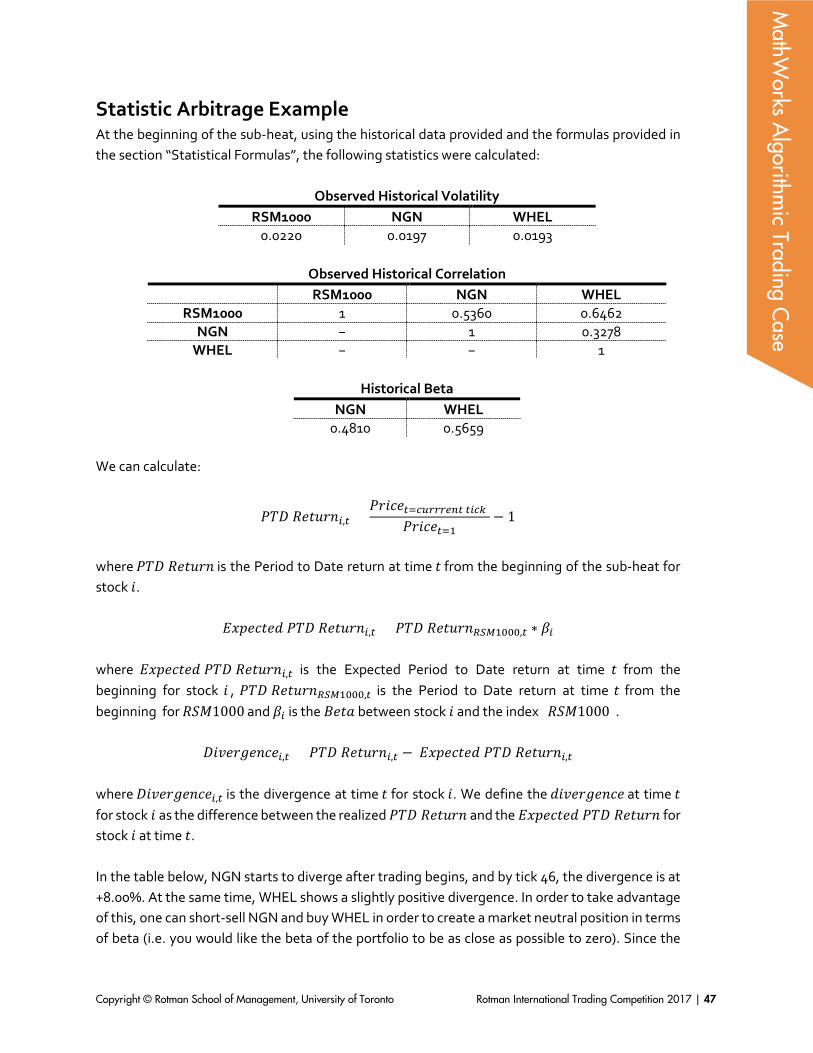
Copyright © Rotman School of Management, University of Toronto Rotman International Trading Competition 2017 | 47
Statistic Arbitrage Example At the beginning of the sub-heat, using the historical data provided and the formulas provided in the section “Statistical Formulas”, the following statistics were calculated:
Observed Historical Volatility RSM1000 NGN WHEL
0.0220 0.0197 0.0193
Observed Historical Correlation RSM1000 NGN WHEL
RSM1000 1 0.5360 0.6462 NGN − 1 0.3278
WHEL − − 1
Historical Beta NGN WHEL
0.4810 0.5659 We can calculate:
𝑃𝑃𝑇𝑇𝐷𝐷 𝑅𝑅𝐸𝐸𝐸𝐸𝑡𝑡𝑡𝑡𝑎𝑎𝑃𝑃,𝑡𝑡 =𝑃𝑃𝑡𝑡𝑅𝑅𝐸𝐸𝐸𝐸𝑡𝑡=𝐴𝐴𝑢𝑢𝑟𝑟𝑟𝑟𝑟𝑟𝑉𝑉𝑛𝑛𝑡𝑡 𝑡𝑡𝑃𝑃𝐴𝐴𝑡𝑡
𝑃𝑃𝑡𝑡𝑅𝑅𝐸𝐸𝐸𝐸𝑡𝑡=1− 1
where 𝑃𝑃𝑇𝑇𝐷𝐷 𝑅𝑅𝐸𝐸𝐸𝐸𝑡𝑡𝑡𝑡𝑎𝑎 is the Period to Date return at time 𝐸𝐸 from the beginning of the sub-heat for stock 𝑅𝑅.
𝐸𝐸𝐸𝐸𝐸𝐸𝐸𝐸𝐸𝐸𝐸𝐸𝐸𝐸𝐸𝐸 𝑃𝑃𝑇𝑇𝐷𝐷 𝑅𝑅𝐸𝐸𝐸𝐸𝑡𝑡𝑡𝑡𝑎𝑎𝑃𝑃,𝑡𝑡 = 𝑃𝑃𝑇𝑇𝐷𝐷 𝑅𝑅𝐸𝐸𝐸𝐸𝑡𝑡𝑡𝑡𝑎𝑎𝑅𝑅𝑅𝑅𝑅𝑅1000,𝑡𝑡 ∗ 𝛽𝛽𝑃𝑃 where 𝐸𝐸𝐸𝐸𝐸𝐸𝐸𝐸𝐸𝐸𝐸𝐸𝐸𝐸𝐸𝐸 𝑃𝑃𝑇𝑇𝐷𝐷 𝑅𝑅𝐸𝐸𝐸𝐸𝑡𝑡𝑡𝑡𝑎𝑎𝑃𝑃,𝑡𝑡 is the Expected Period to Date return at time 𝐸𝐸 from the beginning for stock 𝑅𝑅 , 𝑃𝑃𝑇𝑇𝐷𝐷 𝑅𝑅𝐸𝐸𝐸𝐸𝑡𝑡𝑡𝑡𝑎𝑎𝑅𝑅𝑅𝑅𝑅𝑅1000,𝑡𝑡 is the Period to Date return at time 𝐸𝐸 from the beginning for 𝑅𝑅𝑈𝑈𝑀𝑀1000 and 𝛽𝛽𝑃𝑃 is the 𝐵𝐵𝐸𝐸𝐸𝐸𝑡𝑡 between stock 𝑅𝑅 and the index (𝑅𝑅𝑈𝑈𝑀𝑀1000).
𝐷𝐷𝑅𝑅𝑣𝑣𝐸𝐸𝑡𝑡𝑎𝑎𝐸𝐸𝑎𝑎𝐸𝐸𝐸𝐸𝑃𝑃,𝑡𝑡 = 𝑃𝑃𝑇𝑇𝐷𝐷 𝑅𝑅𝐸𝐸𝐸𝐸𝑡𝑡𝑡𝑡𝑎𝑎𝑃𝑃,𝑡𝑡 − 𝐸𝐸𝐸𝐸𝐸𝐸𝐸𝐸𝐸𝐸𝐸𝐸𝐸𝐸𝐸𝐸 𝑃𝑃𝑇𝑇𝐷𝐷 𝑅𝑅𝐸𝐸𝐸𝐸𝑡𝑡𝑡𝑡𝑎𝑎𝑃𝑃,𝑡𝑡 where 𝐷𝐷𝑅𝑅𝑣𝑣𝐸𝐸𝑡𝑡𝑎𝑎𝐸𝐸𝑎𝑎𝐸𝐸𝐸𝐸𝑃𝑃,𝑡𝑡 is the divergence at time 𝐸𝐸 for stock 𝑅𝑅. We define the 𝐸𝐸𝑅𝑅𝑣𝑣𝐸𝐸𝑡𝑡𝑎𝑎𝐸𝐸𝑎𝑎𝐸𝐸𝐸𝐸 at time 𝐸𝐸 for stock 𝑅𝑅 as the difference between the realized 𝑃𝑃𝑇𝑇𝐷𝐷 𝑅𝑅𝐸𝐸𝐸𝐸𝑡𝑡𝑡𝑡𝑎𝑎 and the 𝐸𝐸𝐸𝐸𝐸𝐸𝐸𝐸𝐸𝐸𝐸𝐸𝐸𝐸𝐸𝐸 𝑃𝑃𝑇𝑇𝐷𝐷 𝑅𝑅𝐸𝐸𝐸𝐸𝑡𝑡𝑡𝑡𝑎𝑎 for stock 𝑅𝑅 at time 𝐸𝐸. In the table below, NGN starts to diverge after trading begins, and by tick 46, the divergence is at +8.00%. At the same time, WHEL shows a slightly positive divergence. In order to take advantage of this, one can short-sell NGN and buy WHEL in order to create a market neutral position in terms of beta (i.e. you would like the beta of the portfolio to be as close as possible to zero). Since the
MathW
orks Algorithm
ic Trading Case

Copyright © Rotman School of Management, University of Toronto Rotman International Trading Competition 2017 | 48
two stocks have different betas, 𝛽𝛽𝑁𝑁𝐺𝐺𝑁𝑁 = 0.4810 and 𝛽𝛽𝑊𝑊𝐻𝐻𝑊𝑊𝑊𝑊 = 0.5659, one may decide to short $10,000 worth of NGN shares (approximately 338 shares) and buy $8,500 worth of WHEL shares (285 shares). The resulting portfolio’s beta (𝛽𝛽𝐺𝐺𝑃𝑃𝑟𝑟𝑡𝑡) will be very close to zero since the ratio is approximately |($𝑣𝑣𝑡𝑡𝑤𝑤𝑡𝑡𝐸𝐸 𝑜𝑜𝑜𝑜 𝑁𝑁𝑁𝑁𝑁𝑁 𝐸𝐸𝑜𝑜𝑠𝑠𝑅𝑅𝐸𝐸𝑅𝑅𝑜𝑜𝑎𝑎)/($ 𝑣𝑣𝑡𝑡𝑤𝑤𝑡𝑡𝐸𝐸 𝑜𝑜𝑜𝑜 𝑑𝑑𝑊𝑊𝐸𝐸𝐿𝐿 𝐸𝐸𝑜𝑜𝑠𝑠𝑅𝑅𝐸𝐸𝑅𝑅𝑜𝑜𝑎𝑎)| = | 𝛽𝛽𝑊𝑊𝐻𝐻𝑊𝑊𝑊𝑊 / 𝛽𝛽𝑁𝑁𝐺𝐺𝑁𝑁 | .
𝑷𝑷𝒓𝒓𝑷𝑷𝑷𝑷𝑷𝑷 𝑷𝑷𝑷𝑷𝑷𝑷 𝑹𝑹𝑷𝑷𝑹𝑹𝑹𝑹𝒓𝒓𝑹𝑹𝑷𝑷,𝑹𝑹 𝑬𝑬𝑬𝑬𝑬𝑬𝑷𝑷𝑷𝑷𝑹𝑹𝑷𝑷𝑬𝑬 𝑷𝑷𝑷𝑷𝑷𝑷 𝑹𝑹𝑷𝑷𝑹𝑹𝑹𝑹𝒓𝒓𝑹𝑹𝑷𝑷,𝑹𝑹
𝑷𝑷𝑷𝑷𝑫𝑫𝑷𝑷𝒓𝒓𝑫𝑫𝑷𝑷𝑹𝑹𝑷𝑷𝑷𝑷𝑷𝑷,𝑹𝑹
Tick RSM 1000
NGN WHEL RSM100
0 NGN WHEL NGN WHEL NGN WHEL
1 35.96 27.04 29.31 − − − − − − −
… … … … … … … … … … …
46 36.78 29.50 29.77 0.0228 0.0910 0.0157 0.0110 0.0129 0.080 0.0028
… … … … … … … … … … …
59 36.18 26.84 29.36 0.0061 -0.0074 0.0017 0.0029 0.0035 -0.0103 -0.0018
When the divergence converges towards zero at tick 59, one can close the position, and the realized profits from the statistical arbitrage will be equal to the arbitrage spread minus commissions:
($29.50 – $26.84) * 338 + ($29.36 – $29.77) * 285 – (338 + 285) * $0.01 * 2 = $769.77
Trading Limits and Transaction Costs
Time of Sub-heat (tick) Gross/Net
1 ~ 299 500,000/100,000
300 0/0
Each trader will be subject to gross and net trading limits during trading in each sub-heat. The gross trading limit reflects the sum of the absolute values of the long and short positions across all securities and the net trading limit reflects the sum of long and short positions such that short positions negate any long positions. Trading limits will be strictly enforced and participants will not be able to exceed them. Each position in stock will be counted towards trading limits with a multiplier of 1 (i.e. if you long 100 shares of any stocks, your gross and the net trading limits will increase by 100).
The maximum trade size will be 10,000 shares per order for stocks. Transaction fees will be set at $0.01 per share for stocks on all market and limit orders filled.
MathW
orks Algorithm
ic Trading Case

Copyright © Rotman School of Management, University of Toronto Rotman International Trading Competition 2017 | 49
Position Close-Out Any non-zero position will be closed out at the end of trading at either the last traded price or the correct price if the stock is experiencing a divergence due to market shock. As such, participants are not required to close statistical arbitrage positions as the sub-heat ends.
Key Objectives Objective 1 Create a model using the provided template to calculate relevant statistical measures between the 3 stocks and non-tradable index. Objective 2 Build a trading algorithm and optimize the trading parameters such that the algorithm efficiently takes advantage of statistical arbitrage opportunities while managing risk exposure and order flow.
MathW
orks Algorithm
ic Trading Case