the role of trading halts in monitoring a specialist marketsgervais/research/... · largely the...
TRANSCRIPT
The Role of Trading Halts in Monitoringa Specialist Market
Roger EdelenUniversity of Pennsylvania
Simon GervaisUniversity of Pennsylvania
When a collection of specialists organize as an exchange, each can reap net privatebenefits at the expense of the exchange by quoting a privately optimal pricing schedule.Coordination makes all specialists and customers better off, but requires a system ofmonitoring and punishment that breaks down when information asymmetries betweenthe exchange and a specialist are high. The specialist may then seek a temporary tradinghalt to alleviate unjustified punishment, or the exchange may halt trading to prevent thequoting of damaging privately optimal pricing schedules. We test this theory on a sampleof NYSE halts. As predicted, we find a significant increase in estimated informationasymmetry immediately preceding trading halts.
Many exchanges are organized and owned by members who perform mostof the market making on the exchange. Such exchanges will seek to max-imize the collective value of all market-maker activities. This study arguesthat trading halts play an important role in that maximization by mitigatingan agency cost inherent in the organizational structure. Individual marketmakers, viewed as the agents operating the exchange, do not always have theincentive to act in the interest of the exchange, the principal in this context.This agency conflict arises whenever the exchange enjoys a reputation fortrade execution quality that is shared by all market makers. As a result ofthis pooled reputation, gouging by one of the exchange’s market makers (e.g.,a substantial, temporary price fade prior to executing a customer’s order) mayresult in a loss of order flow to all of the exchange’s market makers. In some
This article evolved from a previous working paper entitled “Trading Halts in a Principal-Agent Model of anExchange.” Financial support by the Rodney L. White Center for Financial Research is gratefully acknowl-edged. The article owes a great deal to George Sofianos for instrumental discussions at the inception of theproject, and for assistance with its development and data collection. We have benefited from discussions withUtpal Bhattacharya, Peter DeMarzo, James Gallagher, Diego Garcia, Gary Gorton, Joel Hasbrouck, AdityaKaul, Ken Kavajecz, Richard Kihlstrom, John McMahon, Christopher Quick, Duane Seppi, David Shields,Nicholas Souleles, Matt Spiegel, Paul Weller, Donald Wickert, and Bilge Yılmaz. Also providing helpfulcomments and suggestions were Maureen O’Hara, two anonymous referees, and seminar participants at theUniversity of Washington, MIT, Ohio State University, University of Oregon, New York University, DartmouthCollege, Duke University, Temple University, McGill University, Wharton School, the 1998 meetings of theWestern Finance Association, the 1999 NASDAQ-Notre Dame Microstructure conference, the 2000 MarketMicrostructure conference at Yale University, and the 2000 Market Microstructure Meeting of the NBER. Wewould also like to thank Murray Teitelbaum for organizing our visit to the NYSE, and Benjamin Croitoru forhis research assistance. The views and ideas expressed in this article are those of the authors alone. Addresscorrespondence to Simon Gervais, Finance Department, Wharton School, University of Pennsylvania, Stein-berg Hall-Dietrich Hall, Suite 2300, Philadelphia, PA 19104-6367, or e-mail: [email protected].
The Review of Financial Studies Spring 2003 Vol. 16, No. 1, pp. 263–300© 2003 The Society for Financial Studies

The Review of Financial Studies / v 16 n 1 2003
cases, gouging may also lead to sufficient trading profits to outweigh theoffending market maker’s expected loss of future order flow, yet insufficientprofits to also cover the externality imposed on all other market makers. Thusthe exchange suffers an agency cost if market makers cannot be induced tointernalize this externality.The theoretical analysis in this article presumes a specialist-organized
market, where the exchange employs a single market marker, a specialist, foreach stock. In this setting, exchange profits can increase when the specialistscollectively agree to rules and monitoring designed to prevent opportunisticactions. However, given the tremendous amount of stock-specific informa-tion that is surely associated with market making, particularly in the caseof a specialist market, this monitoring can never be perfect. The theoret-ical analysis goes on to show that when monitoring is sufficiently imprecise,punishment becomes a deadweight cost that fails to realign the incentivesof specialists. Trading halts increase exchange profits by eradicating suchno-win scenarios. This motive for halts can explain halts triggered by boththe exchange and the specialist. Halts called by the exchange serve to pro-tect all market-makers’ interests when it is anticipated that an upcoming eventor announcement will compromise the exchange’s ability to cost-effectivelymonitor that stock’s specialist. Halts called by an individual specialist serveto protect that specialist’s interests when monitoring is likely to result in pun-ishment, even when the specialist quotes the efficient pricing schedule givenhis information, that is, that which maximizes expected exchange profits.The two main implications of this analysis are as follows. First, trading
halts should be called by the exchange on some occasions, and solicited bythe specialist on other occasions.1 This empirical fact, previously documentedby Bhattacharya and Spiegel (1998) among others, has not been accountedfor in the theoretical literature. Second, trading halts should be preceded bya substantial increase in the information asymmetry between the exchangeand the specialist regarding the quoted, versus efficient, pricing schedule.Note that this does not refer to information asymmetry about the value ofthe stock, which plays no role in our theoretical analysis. This also is a novelprediction.The empirical analysis in this article tests these predictions. At most
exchanges, monitoring of the market makers involves, among other things,a statistical analysis of trade, quote, and order flow data. From this analysiscomes a hypothesized statement of the efficient price schedule for the marketmaker given existing conditions, and a test of whether the actual quotedschedule violates that norm. Researchers cannot know the statistical proce-dures employed in this evaluation process, indeed, market makers themselveslikely do not know. However, simple statistical estimates of the price impact
1 We say that the specialist solicits, rather than calls, a halt to conform to the rules in effect at the New YorkStock Exchange (NYSE) (our data source). At the NYSE, only a floor official can call a halt, not the specialist.
264

Trading Halts in a Specialist Market
of transactions should provide a useful, observable proxy to the exchange’smonitoring procedure. This proxy approach serves its purpose as long as theexchange tends to lose monitoring precision under the same circumstancesthat our simple estimates lose statistical precision. Since both operate onlargely the same data [we use trading halt and Trade and Quote (TAQ) datafrom the New York Stock Exchange (NYSE) for our estimates], that condi-tion seems likely to hold. We find that the statistical precision of price-impactestimates falls dramatically around NYSE trading halts, a relation that cannotbe fully attributed to patterns in volatility, volume, or the level of the price-impact estimates. This suggests that monitoring uncertainty plays a centralrole in motivating trading halts.A commonly held view of trading halts is that they are designed to reduce
informational asymmetries between traders.2 These asymmetries are reflectedin excessive price volatility [Spiegel and Subrahmanyam (2000)], tradingcrowd uncertainty [Greenwald and Stein (1991)], or transactional risk [Kodresand O’Brien (1994)]. Collectively we refer to these arguments as the levelplaying-field hypothesis. Lee, Ready, and Seguin (1994) examine the effec-tiveness of halts in this regard by comparing the volatility of stocks thatundergo a trading halt to the volatility of stocks with similar characteristicsin similar circumstances but no halt. They find that nonhalting stocks havelower ex post volatility. To the extent that volatility proxies for asymme-tries across traders, this evidence is inconsistent with the level playing-fieldhypothesis. Instead, it suggests that trading halts have perverse effects, as inGrossman (1990) and Subrahmanyam (1994).Halts in our model relate only to the degree of information asymmetry
between the specialist and the exchange. Our model neither predicts nor isinconsistent with the more traditional level playing-field hypothesis. However,monitoring uncertainty, the key variable in our analysis, is likely correlatedwith those variables predicted to be important under the level playing-fieldhypothesis. To clarify inferences, we incorporate those variables into ourempirical analysis. Our results confirm Lee, Ready, and Seguin’s (1994)finding that volatility (liquidity) is unusually high (low) both before and aftertrading halts. However, because the unusual monitoring uncertainty observedjust before trading halts cannot be attributed to excess volatility, our empir-ical analysis suggests that the control sample constructed by Lee, Ready,and Seguin (1994) does not fully replicate market conditions around actualtrading halts. Our evidence suggests that a halt was called in one case, andnot in the other, because there was a greater erosion in the exchange’s abilityto monitor in the one case.
2 Halts in individual-stock trading differ from market-wide circuit breakers. Halts are called subjectively inresponse to that stock’s market conditions; circuit breakers go into effect objectively, generally as a result ofexcessive price moves. This difference has often been neglected by the literature on trading halts; an exceptionis the work by Subrahmanyam (1995).
265

The Review of Financial Studies / v 16 n 1 2003
There has been considerable debate about the role of trading halts and cir-cuit breakers. This debate is part of a more general polemic in which lawyersand economists have made arguments for and against the self-regulation ofsecurities exchanges. For example, Fischel and Grossman (1984), Fischel(1986), Kyle (1988), Miller (1991), and Mahoney (1997) all argue that excha-nges have the proper economic incentives to adopt rules and regulationsmeant to benefit their customers (i.e., investors). These incentives revolvearound the reputation effects of low-quality transaction services and dis-orderly markets, and the competition (for transaction volume) from otherexchanges. In these authors’ view, external (e.g., government) regulation willsimply muddle these clear incentives. The opposite view is best character-ized by Pirrong (1995), who argues that self-regulation is unlikely to resultin efficient outcomes for two reasons: (1) exchanges cannot possibly inter-nalize the full effects of disorderly markets; and (2) exchange competitionis, in reality, less intense than what is required for the above incentive argu-ments to work. For these reasons, Pirrong (1995) advocates external regula-tion instead of self-regulation. Our view in this article is best approximatedby Kyle (1988), who advocates the use of trading halts in the self-regulationof an exchange. However, the underlying reason for halting in our study isprofoundly different from that in Kyle’s discussion. Our article also relatesto DeMarzo, Fishman, and Hagerty’s (2000) exploration of the policies thatself-regulatory organizations implement to monitor their members. The pos-sibility that halting can enhance monitoring, our principal concern in thisarticle, is not investigated by these authors.Our empirical work differs considerably from most previous empirical
work on trading halts, in the sense that it concentrates on the causes of tradinghalts and not their effects. For example, Hopewell and Schwartz (1978),Kryzanowski (1979), King, Pownall, and Waymire (1992), and Wu (1998) allstudy the price discovery process before, during, and/or after trading halts.Our work is mostly about the triggers of such halts. In that respect, it isclosely related to Lee, Ready, and Seguin (1994), and to Bhattacharya andSpiegel (1998), but as discussed above, it argues for a related but differenthalt trigger.In terms of the forces at play, our article more generally relates to two
strands of the economics literature. First we can think of the confidence ofan exchange’s customers as a public good that can be “polluted” by anyof the specialists for their own private benefit.3 Following Pigou (1932),Buchanan (1969), and Baumol (1972), among many others, our objectiveis to find an optimal way for the exchange to control these negative exter-nalities. The postulated mechanism is similar to those documented by theaforementioned authors in that a corrective tax is assessed on the deviatingagents. Alternatively, we can think of an exchange’s group of specialists as a
3 This analogy was pointed out by an anonymous referee.
266
Trading Halts in a Specialist Market
team whose objective is to maximize total profits. Absent coordinating mech-anisms, however, the team members are tempted to deviate and free ride onthe good will of others. Like Groves (1973), Holmstrom (1982), and Kandeland Lazear (1992), we develop a system of incentives designed to enhanceteam behavior. Our approach differs slightly from the above literature in thatthe peculiar structure of specialist markets leads us to introduce the possi-bility for either the monitor or the monitoree to “pull the plug” (i.e., to calla halt) when the mechanisms in place do not perform as well as they should.Our article is organized as follows. In Section 1 we develop a model in
which an exchange consists of many stocks, the market in each of whichis made by an assigned specialist. This section also shows how the incen-tives of these specialists can conflict with those of the exchange as a whole.Section 2 shows how an appropriate system of monitoring involving tradinghalts helps reconcile these conflicts. The empirical predictions of the modelare developed in Section 3. In Section 4 we describe the data used in ourempirical analysis and present the tests of the model. Concluding remarksare presented in Section 5.
1. The Model
1.1 The basic setupConsider an exchange on which N stocks are traded for a large (possiblyinfinite) number of periods. We assume that the market-making activitiesfor each stock i = 1� � � � �N are performed by a different specialist i. Thus,in every period, the specialist for stock i quotes a price schedule whichspecifies the price at which he is willing to accommodate trades of differentsizes. Specialists are assumed to be risk neutral and so seek to maximize theexpected profits that their own market-making activities generate. Throughoutthe article, we refer to the exchange as the set of all N specialists gathered inthis one trading venue. Alternatively the exchange can be viewed as a thirdparty sharing the specialists’ profits.4
The customers of an exchange typically trade in many stocks, and theytypically have alternative venues where they can execute those trades. Weassume that the customers’ choice of trading venue is not made solely at thelevel of individual stocks, but partly at the exchange level. That is to say,customers assess the performance of an exchange by computing the averageperformance of every specialist on the exchange. A bad experience with anyone specialist negatively affects a customer’s overall likelihood of choosingthat exchange for any of his subsequent trades (including those of differentstocks). The idea is that a bad fill of an order implies that the exchange has
4 For example, the NYSE collects fees from its specialists in exchange for the right to make a market. Thesefees come in the form of a fraction of the total trade volume handled by each specialist, in addition to a fixedannual fee. Modeling these fees explicitly would add little to the economics of the article.
267

The Review of Financial Studies / v 16 n 1 2003
insufficient checks and monitors in place, which in turn implies that anotherbad fill is likely even if the order goes to a different specialist. In fact, thisline of thought is well captured by the following passage from Fischel andGrossman (1984, p. 293):
[T]he existence of fraud on the exchange will discourage customer par-ticipation with all members; it will lead customers to trade with otherexchanges which have a better reputation for preventing member fraud.
In other words, the occurrence (or even perception) of gouging anywhere onthe exchange will tend to alienate at least some investors against the exchangeas a whole. This investor dissatisfaction could take many forms, for example,a reduction of order flow from existing customers or a loss of new customersor listings because of bad publicity.More specifically, let us assume that, in a given period, specialist i can
quote either a conservative price schedule or an aggressive price schedule.We denote the event in which specialist i quotes a conservative (aggressive)price schedule by �̃i =G (�̃i =B), where the use of G (B) is meant to capturethe fact that the conservative (aggressive) price schedule will be good (bad)from the exchange’s point of view. The conservative and aggressive priceschedules lead to expected profits of a > 0 and 2a, respectively, for thespecialist. However, the aggressive price schedule is perceived as gougingby the customer and, as a result, imposes a negative externality of c onthe whole exchange.5 This externality is borne equally by each of the Nspecialists, leading to a reduction of c
Nin each’s expected profits for the
period. For reasons to be made clear later, we assume that
c
N< a < 2a < c� (1)
We restrict the specialists’ action space to only two price schedules in orderto simplify the analysis. A larger action space would include price schedulesthat lead to many different specialist profits and negative externalities, butwould leave the economic forces at play largely the same. Also, practicallyspeaking, the conservative and aggressive price schedules are likely to changefrom period to period, as they both depend on the prevailing market condi-tions. For modeling purposes, however, we can abstract from that, as ourresults only depend on the fact that different price schedules are preferredby the exchange (the conservative schedule) and individual specialists leftunsupervised (the aggressive schedule). Similarly the decision not to specifythe customers’ motives for trading allows us to concentrate on the relation-ship between the exchange and the specialists, and not on the relationshipbetween the specialist and the traders. Incidentally, this is why our model has
5 This negative externality can be interpreted as the present value of all the costs imposed by traders on theexchange following a period of aggressive behavior by a specialist.
268
Trading Halts in a Specialist Market
little to say about the level playing-field hypothesis, which directly resultsfrom the interactions between specialists and traders.Before we proceed to analyze the equilibrium to this model, we want to
emphasize that our reduced-form model seeks to capture an aspect of anexchange that is often overlooked in microstructure models: market makerswho band together to form an exchange do not operate independently. Anessential characteristic of an exchange is the pooling of market-makers’ rep-utations. This necessarily implies that a specialist’s actions in one stock canaffect the market for other, seemingly unrelated stocks.
1.2 Incentives and the impossibility of cooperationIn this model, all periods are similar but they are independent from oneanother. Our analysis therefore concentrates on just one of those periods. Letus denote the profits of specialist i in any given period by �̃i. These profitscome from direct market-making activities (�̃i), which are reduced by thenegative externalities imposed on specialist i by the other specialists (�̃ij ,j �= i):
�̃i = �̃i−N∑j=1j �=i
�̃ij �
We incorporate the negative externalities that specialist i imposes on him-self into his direct profits �̃i. The setup of Section 1.1 means that
E[�̃i��̃i =G
] = a�
E[�̃i��̃i = B
] = 2a− c
N�
E[�̃ij ��̃j =G
] = 0� and
E[�̃ij ��̃j = B
] = c
N�
Specialist i’s price schedule only affects his direct profits. His choice of aprice schedule will therefore be the same irrespective of how he expectsthe other specialists to quote, and his decision to quote conservatively oraggressively comes down to a comparison of his expected direct profits undereach alternative:
E[�̃i��̃i = B
]−E[�̃i��̃i =G
]=
E
[�̃i��̃i = B
]− N∑j=1j �=i
E[�̃ij
]−E
[�̃i��̃i =G
]− N∑j=1j �=i
E[�̃ij
]= E
[�̃i��̃i = B
]−E[�̃i��̃i =G
]= a− c
N> 0�
269
The Review of Financial Studies / v 16 n 1 2003
This last inequality, which obtains from Equation (1), reflects the fact that thespecialist only absorbs a fraction 1
Nof the externalities that he imposes on the
exchange. Since specialist i cannot affect the negative externalities imposedon him by the other specialists, he will choose to quote the aggressive priceschedule, as will every other specialist. As a result, E��̃ij = E��̃ij ��̃j = B=cNfor all i �= j and, in equilibrium,
E[�̃i
]= E[�̃i��̃1 = · · · = �̃N = B
]= 2a− c
N− N −1�
c
N= 2a− c� (2)
Suppose instead that the specialists somehow coordinate so that all quote aconservative price schedule. In that case, no negative externalities are createdand the expected profits of each specialist are given by
E[�̃i
]= E[�̃i��̃1 = · · · = �̃N =G
]= a > 2a− c�
where the last inequality follows from Equation (1). Therefore all specialistswould be better off if they could each agree to be conservative, but such coor-dination is impossible, given the incentives of each. In effect, the reputationof the exchange vis-à-vis its customers is a “public good” for the specialists.Without coordination incentives, every specialist is tempted to free ride onthe goodwill of the other specialists. Clearly the specialists and the exchangeas a whole stand to gain from implementing mechanisms that will mitigatethis free-rider problem.
2. Monitoring and Trading Halts
This section shows how a combination of monitoring and trading halts canhelp reduce the coordination problem of the exchange. The first-best sce-nario for the exchange and its specialists is perfect coordination, in whichevery specialist quotes a conservative price schedule. If the exchange is ableto observe each specialist’s price schedule perfectly, this first-best scenarioobtains with a simple monitoring scheme involving large punishments foraggressive price schedules.Perfect monitoring is unrealistic. With his unique position as an interme-
diary for every trade in a particular stock, the specialist has intimate knowl-edge of the order flow, trading crowd, and general activity in that stock.6
That knowledge allows the specialist to assess both the price schedule thatwould satisfy the exchange’s coordination requirements (in our model, theconservative price schedule) and the potential for opportunistic actions (i.e.,the private gain from quoting an aggressive price schedule). It strains cred-ibility to assert that the exchange could match this information set for each
6 For example, the relationship between the specialist and the exchange’s customers is at the heart of Benveniste,Marcus, and Wilhelm’s (1992) market-making model.
270
Trading Halts in a Specialist Market
of the specialists, at any cost. Yet to assess with perfect accuracy whethera specialist’s actions on a particular trade are abusive, the exchange musthave the same information as the specialist. Realistically the exchange relieson statistics and surveys to evaluate the performance of each specialist. Thisinformation is a strict subset of the specialists’, making any kind of moni-toring imperfect.We capture these effects in our reduced-form model by assuming that the
exchange can only imperfectly observe the specialist’s quoted price schedule.7
Specifically we assume that at the end of every period the exchange receivesa signal �̃i, which provides incomplete information about �̃i. The precision ofthis signal p̃i ∈ �0� 1
2 is random and independently redrawn in every period:8
�̃i�(�̃i = B
) ={B� Pr 1
2 + p̃i
G� Pr 12 − p̃i�
(3)
�̃i�(�̃i =G
) ={G� Pr 1
2 + p̃i
B� Pr 12 − p̃i�
(4)
Notice that the exchange finds out the exact strategy adopted by the specialistwhen p̃i = 1
2 , but is just as likely to be right as wrong when p̃i = 0. Wesay that the exchange has relatively precise (imprecise) knowledge of theefficiency of specialist i’s price schedule when p̃i is close to 1
2 (0).9 Foranalytical convenience, we also assume that p̃i is uniformly distributed onthe �0� 1
2 interval.The precision p̃i is the (inverse-)level of information asymmetry between
the exchange and specialist i. We assume that the specialist knows p̃i at thebeginning of every period, whereas the exchange knows p̃i at the beginningof the period only with probability q ∈ �0�1. Allowing q to be smaller thanone captures the fact that the exchange is sometimes unaware of how wellit will be able to assess the specialist in the future. While this assumptionenhances the applicability and generality of our model, it will become clearlater that it does not affect any of our results.
7 In our model, price schedules are either conservative or aggressive, and it is common knowledge that theexchange prefers the conservative schedule. The only uncertainty for the exchange is whether or not thespecialist quoted it. In practice, the problem of determining the “conservative” (i.e., efficient) price scheduleis itself probably just as difficult as that of inferring whether or not the specialist quoted it. We suspect thata simple modification to the model would facilitate this extra layer of uncertainty without altering our basicresults. However, the added complexity (two sources of uncertainty as opposed to just one) would not addany intuition. We will come back to this issue in our empirical analysis.
8 The assumption that p̃i is independent across periods is made for tractability purposes: it allows us to treatone period at a time. In general, we should expect the precision process to be autocorrelated. As our analysiswill make clear, the main predictions of the model would be unaffected with this more general structure.
9 In what follows, we assume that this is all the information that the exchange can use, that is, we interpret �̃ias the total ex post information of the exchange. In particular, we assume that this information includes theprior distribution for the price schedule �̃i quoted by the specialist in equilibrium.
271
The Review of Financial Studies / v 16 n 1 2003
2.1 MonitoringWe assume that monitoring takes the form of an ex post evaluation of the spe-cialist’s performance based on the exchange’s information. More precisely,since the aggressive price schedule is detrimental to the exchange, we assumethat the exchange systematically punishes specialist i if it observes �̃i = B.The penalty ̃i is a fine of � > 0 imposed at the end of the period, where� is determined at the outset by the exchange.10 In practice, this penalty isrelated to the overall performance of the specialist and can take on manyforms ranging from a dollar fine to a loss of the specialist’s seat on theexchange. More commonly, the penalty results in the exchange not consid-ering the specialist in the assignment of new stocks, a topic analyzed byCorwin (1999).The monitoring scheme is not perfect given that the exchange does not
have perfect information about the specialist’s actions during the period.Indeed, it is possible that �̃i = B when �̃i =G, so that the specialist is pun-ished even after quoting the efficient price schedule. Similarly it is possiblethat �̃i =G when �̃i = B, so that the specialist can get away with customergouging. Nevertheless, it is clear from Equations (3) and (4) that the spe-cialist is more likely to be punished when he quotes an aggressive priceschedule than when he quotes a conservative schedule. Indeed,
E[ ̃i��̃i = B� p̃i
]= �
(12+ p̃i
)≥ �
(12− p̃i
)= E
[ ̃i��̃i =G� p̃i
]�
We assume that any tax paid by a specialist to the exchange is a dead-weight loss to both the exchange and the specialist, that is, it is not possibleto redistribute the tax. Realistically, monitoring is costly. For example, theNYSE incurs costs in the form of computer equipment and human resourcesfor its electronic supervision system, StockWatch. In that sense, our assump-tion of a deadweight tax amounts to saying that the monitoring scheme isexactly financed by the taxes that it charges. This assumption also ties inwith the work of Fischel and Grossman (1984) and Mahoney (1997), whopoint out that the value of self-regulation should be analyzed as a trade-offbetween the benefits that it generates and the costs that it involves. As wediscuss later, the choice of � by the exchange should reflect that trade-off.Since the exchange is, ultimately, just a collection of specialists, it is rele-
vant to ask whether specialists will agree to monitoring ex ante (that is, priorto the exchange or any specialist learning p̃i, i = 1� � � � �N , at the beginningof the first period). As it turns out, the answer depends on the pro rata exter-nality that gouging creates, c
N. If that quantity is sufficiently small, then there
can be cases where the specialists would decline to implement the monitoringscheme. This is because the specialists only incur a small fraction of the neg-ative externality that they cause when quoting an aggressive price schedule,
10 We also refer to this penalty as a tax, following Pigou (1932).
272
Trading Halts in a Specialist Market
so that the extra profits that they can generate for themselves are enough tocover the punishments associated with the monitoring scheme. Increasing thepotential punishment � does not solve the problem, as large ex ante expectedtaxes would render the market-making activities of the specialists completelyunprofitable: the specialists would simply refuse to be monitored.At the beginning of every period, specialists decide on a price schedule for
the period. Since punishment is more likely when they quote aggressively, itis no longer the case that they will always prefer aggressive price schedules,as in Section 1.2. As before, no specialist can affect the externalities thatothers will impose on them. So every specialist decides on a price schedulebased on the expected profits that directly result from their market-makingactivities and on the expected punishment that this schedule brings about.Before quoting his price schedule, the specialist also knows p̃i, the precisionof the exchange’s ex post monitoring. Therefore his quoting decision is basedon a comparison between E��̃i− ̃i��̃i =G� p̃i and E��̃i− ̃i��̃i = B� p̃i.If specialist i quotes a conservative schedule, then his direct expected
profits for the period are given by
E[�̃i− ̃i��̃i =G� p̃i
]= a−�
(12− p̃i
)� (5)
If instead he quotes an aggressive price schedule, then his direct expectedprofits for the period are
E[�̃i− ̃i��̃i = B� p̃i
]= 2a− c
N−�
(12+ p̃i
)= a+�−�
(12+ p̃i
)� (6)
where we have defined � ≡ a− cN> 0 as the net personal gain to gouging.
The following lemma results from a simple comparison of Equations (5)and (6).
Lemma 1. Under monitoring, specialist i will quote a conservative priceschedule (�̃i =G) if
p̃i >�
2�� (7)
and an aggressive price schedule (�̃i = B) otherwise.
The specialist will choose to be conservative when the chance of theexchange making an incorrect inference of his actions is slight (i.e., highp̃i), when the punishment is high, or when the net benefit to gouging issmall. Otherwise the increase in expected punishment when an aggressiveprice schedule is quoted is not sufficiently large to deter the specialist fromreaping the gains of gouging the customer.Note that setting � to a value smaller than � does not affect the incentives
of the specialists. Since p̃i ∈ �0� 12 , it can then never exceed �
2� , as required
273

The Review of Financial Studies / v 16 n 1 2003
by Equation (7). This is why we always restrict � to be larger than � inwhat follows. Also, while Equation (7) seems to indicate that setting � toa large value induces the specialist i to quote a conservative price schedulemost of the time, a large � is not the solution to the coordination problempresented in Section 1.2. A large � means that the specialist will be punishedseverely when the exchange observes �̃i = B. Since this can happen evenwhen the specialist’s actions are conservative, the ex ante expected valueof punishments might be sufficiently large that the specialist simply refusesto be monitored. Recall that ex ante expected profits are 2a− c withoutmonitoring. An acceptable � cannot cause ex ante expected profits to fallbelow this amount. The following result will help us assess the effectivenessof the monitoring scheme.
Lemma 2. Suppose that the exchange and the specialists adopt the moni-toring scheme with some � > �. The ex ante expected profits of specialist iin any given period are then given by
E��̃i= a
(1− �
�
)+ 2a− c�
�
�−
(�
4+ �2
2�
)� (8)
This last result illustrates the monitoring trade-off. As � increases, moreweight is put on the coordinated expected profits a and less weight is puton the gouging outcome, 2a−c. However, for � >
√2�, better coordination
comes at a price: the expected deadweight punishments, as represented by thelast term in Equation (8), are increasing in �. The value of monitoring cantherefore only be assessed by comparing the specialists’ ex ante expectedprofits with and without it. If there exists a � > � such that monitoringimproves these expected profits, the exchange and the specialists will bewilling to adopt monitoring. Otherwise, monitoring alone is not sufficientto solve the coordination problem of Section 1.2. The following propositionassesses these possibilities.
Proposition 1. The exchange and the specialists will agree ex ante to adoptmonitoring if the net benefit to gouging, �, is sufficiently small. It is possiblethat the exchange and the specialists cannot agree to adopt monitoring if theself-imposed externality from gouging, c
N, is sufficiently small.
This last result suggests that monitoring alone is not optimal in manyplausible circumstances. In particular, since �= a− c
N, N must be relatively
small for monitoring alone to be both acceptable and effective. Intuitively,when N is large, specialists only absorb a small fraction 1
Nof the negative
externalities that they generate. As a result, a large punishment is needed torealign their objectives with those of the exchange. Thus, with large N , thespecialists face a choice of two losing propositions: incur a lot of externalitycosts or incur rampant punishment. Although increasing � reduces the nega-tive externalities borne by the exchange through better specialist coordination,
274
Trading Halts in a Specialist Market
the deadweight taxes associated with monitoring exceed these reductions andturn monitoring into a losing proposition. In the remainder of the analysis weshow that trading halts improve specialists (and exchange) profits in all sit-uations, in particular in this all-too-likely situation where monitoring wouldnot be acceptable.
2.2 Trading haltsAs discussed in Section 2.1, monitoring alone may not be a very useful, oracceptable, approach to reducing the specialists’ externality problem. There isa second problem with this approach. Even if the specialists do agree ex anteto the scheme of monitoring (alone) proposed in Section 2.1, they (and theexchange) nevertheless face isolated periods where monitoring and punishingdoes more harm than good. Suppose for example that � is sufficiently smallto make monitoring ex ante agreeable. In some periods (as we will soonshow), upon learning p̃i, specialist i may find himself in a position where anyquoting decision leads to negative expected profits: an aggressive scheduledoes not produce sufficient gouging profits to recoup expected fines, yet aconservative quote also has a strong chance of generating a fine. In thesecircumstances the option to halt trading rather than post a price scheduleallows the specialist to credibly signal to the exchange that he cannot performhis market-making duties diligently yet profitably.A similar situation could arise for the exchange. Recall that, in our model,
the exchange learns p̃i with probability q at the beginning of every period.In some periods it will learn that its precision, p̃i, is small. This might cor-respond to, for example, a listed company warning the exchange that, due toidiosyncratic events at the firm (e.g., a pending merger announcement), thepotential for informed trading in that company’s stock is currently extremelyhigh. That information tells the exchange that it will be very difficult to dis-tinguish gouging from efficient pricing ex post. When the specialist learns ofthe situation (i.e., observes p̃i), he sees an opportunity to gouge with littlefear of getting caught. The option to halt trading and reopen with a call auc-tion lets the exchange protect its reputation in these vulnerable moments oftrading that stock.So let us assume that upon learning p̃i the exchange has the option to halt
stock i before the specialist is allowed to quote a price schedule, and thatspecialist i has the option of halting instead of quoting a price schedule.11
In both cases, the halt results in zero profits for specialist i, with no exter-nality imposed on the other specialists.12 The specialist’s problem is similarto that analyzed in Section 2.1, except that he now has the option to halt.The specialist will exercise this option whenever his expected profits are
11 We assume that halting without knowing p̃i is never optimal for the exchange. Otherwise, closing the exchangealtogether would be the best alternative.
12 Of course, in reality, the halt itself may impose some externality as well [Grossman (1990)]. The importantissue is that halting causes less of an externality than continuous trading in these situations. Without loss ofgenerality, the model simply assumes that no externality is caused by halts.
275
The Review of Financial Studies / v 16 n 1 2003
negative with both the conservative and aggressive price schedule. The fol-lowing lemma summarizes this.
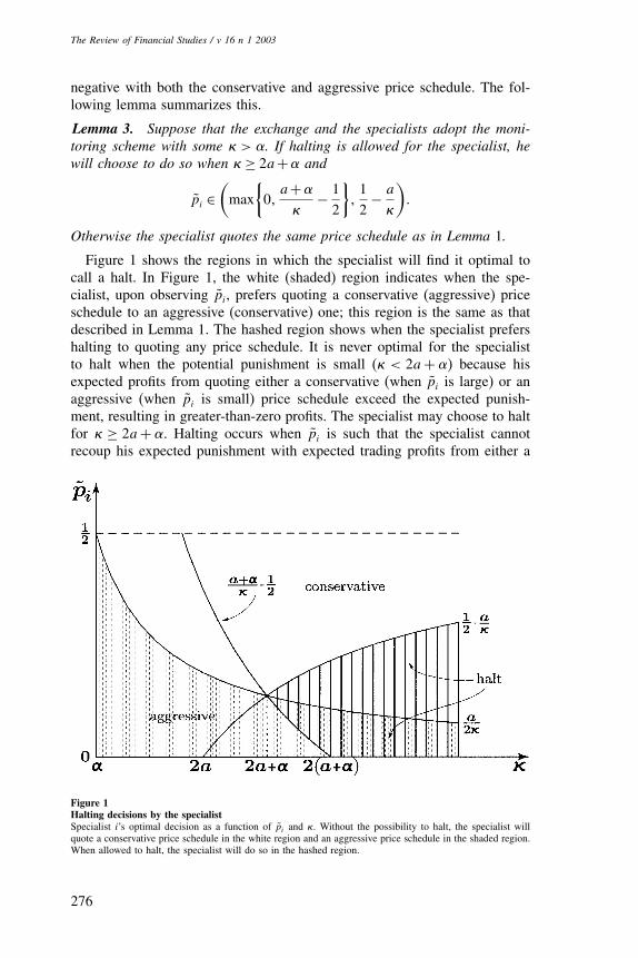
Lemma 3. Suppose that the exchange and the specialists adopt the moni-toring scheme with some � > �. If halting is allowed for the specialist, hewill choose to do so when �≥ 2a+� and
p̃i ∈(max
{0�
a+�
�− 1
2
}�12− a
�
)�
Otherwise the specialist quotes the same price schedule as in Lemma 1.
Figure 1 shows the regions in which the specialist will find it optimal tocall a halt. In Figure 1, the white (shaded) region indicates when the spe-cialist, upon observing p̃i, prefers quoting a conservative (aggressive) priceschedule to an aggressive (conservative) one; this region is the same as thatdescribed in Lemma 1. The hashed region shows when the specialist prefershalting to quoting any price schedule. It is never optimal for the specialistto halt when the potential punishment is small (� < 2a+�) because hisexpected profits from quoting either a conservative (when p̃i is large) or anaggressive (when p̃i is small) price schedule exceed the expected punish-ment, resulting in greater-than-zero profits. The specialist may choose to haltfor � ≥ 2a+�. Halting occurs when p̃i is such that the specialist cannotrecoup his expected punishment with expected trading profits from either a
Figure 1Halting decisions by the specialistSpecialist i’s optimal decision as a function of p̃i and �. Without the possibility to halt, the specialist willquote a conservative price schedule in the white region and an aggressive price schedule in the shaded region.When allowed to halt, the specialist will do so in the hashed region.
276
Trading Halts in a Specialist Market
conservative or aggressive price schedule. Small values of p̃i in the conser-vative range increase the likelihood of undue punishment, and large valuesin the aggressive range increase the likelihood that the specialist is caughtgouging. Both imply negative profits.With probability q, the exchange observes p̃i before the specialist makes
his quoting decision. When this observation implies that the specialist willquote aggressively, the exchange halts trading in stock i (recall that aggressiveprice schedules are by definition detrimental to the exchange). The nonhashedshaded region of Figure 1 indicates the parameter combinations in which theexchange calls a halt, conditional on having observed p̃i. Note that noneof the results of our model depend on the value of q. Assuming that theexchange sometimes observes its monitoring precision before the specialistonly serves to illustrate that halting has a dual purpose in the presence ofmonitoring: it allows the specialists to avoid excessive punishments, and itallows the exchange to prevent opportunistic actions by the specialist whenmonitoring is difficult.Lemma 3 and the above discussion show that halting is at times optimal
for the specialist or the exchange in the presence of monitoring. However,we have not shown that specialists will find the monitoring-halting schemeacceptable in the first place. This is far from obvious, as granting the exchangehalting rights may prevent the specialist from making (potentially large)trading profits. The rest of this section shows that incorporating halts intothe monitoring scheme causes monitoring to always be accepted by special-ists, even in cases where they otherwise would not find it acceptable. Thefollowing lemma is the analogue to Lemma 2 when halting is allowed.
Lemma 4. Suppose that the exchange and the specialists adopt the mon-itoring scheme with some � > �, and that halting is allowed for both theexchange and the specialist. The ex ante expected profits of specialist i inany period are then given by
E��̃i=
a
(1− �
�
)+ 1−q�2a− c�
�
�
− �
4− �2
2�+q
�
2
(1+ �
2�
)if � ∈ ��2a+��
2a2
�+ 1−q�2a− c�
[2a+��
�−1
]
− a2
�− 1−q�
[a+��2
�− �
4
]if � ∈ �2a+��2a+��
a2
�if � ∈ 2a+������
(9)
277
The Review of Financial Studies / v 16 n 1 2003
We need to verify that the specialists’ expected profits are improved whenhalting is possible. We establish this in two parts. First, we show that thehalting option always improves the ex ante expected profits of the specialistsunder any monitoring scheme with �> �. We then show that there is alwaysat least one monitoring scheme �>� which the exchange and the specialistscan agree upon ex ante. In fact, the existence of this monitoring schemedoes not depend on any parameter of the model. The following propositionestablishes the first part.
Proposition 2. Suppose that the exchange and the specialists adopt themonitoring scheme with some �>�. The exchange and the specialists alwaysprefer this monitoring scheme when it is complemented with the possibilityfor either to halt trading.
This result captures the essence of the role for trading halts in this multi-specialist model of an exchange: in the presence of information asymmetriesbetween the exchange and its specialists, the effect of monitoring is alwaysimproved by allowing the different parties to halt trading in a stock. Noticethat, unlike other models of trading halts, our model does not require excessvolatility or an extreme informational event for a halt to be called. Instead,trading halts are simply a mechanism to enhance the effectiveness of mon-itoring.13 The next proposition shows that this enhancement is so great thatit eliminates the situation where specialists would rather accept the exter-nality than instigate monitoring. Also, trading halts in our model are theresult of optimal decisions made by the exchange or the specialists: they arenot alternatives to market breakdowns [see, e.g., Bhattacharya and Spiegel(1991) and Spiegel and Subrahmanyam (2000)] or exogenous mechanisms toreimplement dominating equilibria [see, e.g., Kumar and Seppi (1994)].
Proposition 3. As long as halting is allowed for both the exchange and thespecialists, there exists a � > � such that the exchange and the specialistsagree ex ante to monitoring.
This result is quite important. Proposition 1 shows that it may be the casethat the deadweight loss of punishment through monitoring (without the pos-sibility to halt) exceeds the reduction of externalities for any �. Propositions 2and 3 tell us that, not only is it the case that trading halts make monitoringbetter for both the exchange and the specialists, but it is also the case thattrading halts always make monitoring optimal.Although not shown in Proposition 3, the exchange and the specialists
can agree to monitoring for many values of �. These different values forspecialist punishment will imply different frequencies of trading halts and
13 Of course, excess volatility or extreme information events would probably increase the information asym-metries between the exchange and the specialists, and so would be associated with more halts than regularsituations. But they are certainly not necessary for halts to occur.
278

Trading Halts in a Specialist Market
punishment, as well as different expected deadweight punishments. As men-tioned in Section 2.1, assuming that punishments are deadweight losses isessentially equivalent to assuming that the cost of monitoring is coveredby the punishments that are paid by the specialists. The fact that differentvalues of � can be agreed upon leaves an additional degree of freedom forthe exchange to set up a monitoring scheme that it can finance.
3. Empirical Implications
The central insight from the model is that trading halts can play an impor-tant role in the monitoring process that is critical to a specialist-organizedexchange. In particular, trading halts come into play when information asym-metries between the exchange and the specialists render monitoring inef-fective. In our model, this information asymmetry is captured by p̃i, theprobability that the exchange will correctly monitor the specialist in a givenperiod.
Proposition 4. The expected value of p̃i conditional on a halt being calledfor stock i is smaller than its unconditional expected value.
There is no direct empirical analog to p̃i. However, its essence is clear. Tomake this proposition testable, we rephrase it as follows.
Implication 1. Around a trading halt for a stock, the exchange will havemore difficulty measuring the actions (and the appropriateness of those act-ions) taken by the stock’s specialist than at other times.
Practically speaking, given the number of specialists and stocks on anexchange, statistics gathered by the exchange throughout the trading processwill play an important role in assessing the actions of the specialists. Thissets up our main empirical test: we replicate this statistical analysis, greatlysimplified, and use the precision from that statistical analysis as our testvariable.In the model, the exchange always prefers that the specialists quote a con-
servative price schedule, that is, the efficient schedule for the exchange. Thisefficient schedule is fixed and common knowledge; it is the actual quotedschedule that is assumed known with asymmetric precision. In practice,asymmetric information about the efficient schedule itself seems at least aslikely as asymmetric information about the specialist’s quoted schedule. Theefficient schedule depends on minutely detailed, constantly changing infor-mation about market conditions, trader identity, etc. Because specialists get toknow the behavior of their customers over time, both through careful observa-tion of the order flow and direct communication, their conditional knowledgeof the efficient schedule is likely substantial. The exchange cannot possiblymatch the richness of the information sets possessed by the hundreds of spe-cialists it must monitor. As a result, the exchange’s conditional information
279
The Review of Financial Studies / v 16 n 1 2003
about the efficient schedule is relatively sparse. In our tests of the modelwe take the view that uncertainties about both the efficient schedule andthe quoted schedule are relevant in measuring the precision with which theexchange can assess the actions of the specialists.A second theoretical innovation of our model is that trading halts result
from decisions made by the exchange or the specialists. This yields a secondtestable implication.
Implication 2. Trading halts should be called by the exchange in somecases and by specialists in other cases.
Bhattacharya and Spiegel (1998) document in their empirical study ofNYSE trading halts between 1974 and 1988 that about 50% of trading haltsare news dissemination halts, and about 50% are order imbalance halts. Ourdata suggest a 25–75% breakdown for 1993 and 1994.14 Typically news dis-semination halts are called by the exchange upon learning that a news eventis about to affect the value of a stock. On the other hand, order imbalancehalts are usually called (or more precisely requested) by a specialist whoobserves unusual trading activity in his stock. Implication 2 is supported bythese observations.Proposition 4 and Implication 1 do not depend on whether the halt was
called by the exchange or the specialist. Yet we know from Section 2.2 thatexchange-called halts will occur when the exchange expects the specialist toquote an aggressive price schedule. According to Figure 1, this will happenwhen p̃i is close to zero. Specialist-called halts, on the other hand, can occurfor intermediate values of p̃i; indeed, for �∈ �2a+��2a+��, the specialistwill choose to quote an aggressive price schedule when p̃i is between
a+��
− 12
and 12 − a
�. This leads to the following result.
Proposition 5. The expected value of p̃i conditional on a halt being calledby the exchange for stock i is smaller than its expected value conditional ona halt being called by specialist i.
Again, this result is not directly testable, but it can be rephrased accordingto the essence of p̃i to yield the following implication.
Implication 3. The precision of statistical estimates of the specialist’s act-ions (and the appropriateness of those actions given market conditions) islower around exchange-called trading halts (e.g., news dissemination) thanaround specialists-called trading halts (e.g., order imbalance).
In the remainder of the article we test these implications using a sampleof NYSE halts for the years 1993 and 1994, along with trade and quote datafor the same two years.
14 This will be documented later in Table 1.
280
Trading Halts in a Specialist Market
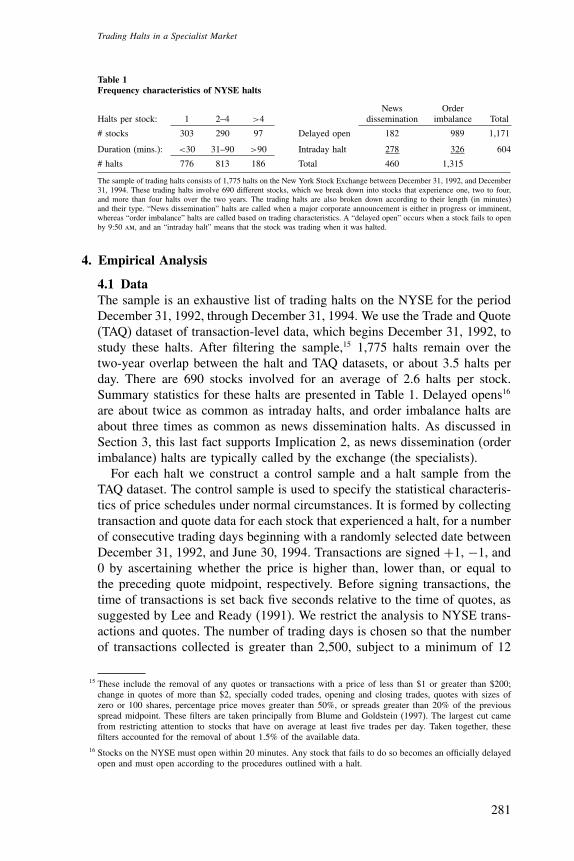
Table 1Frequency characteristics of NYSE halts
News OrderHalts per stock: 1 2–4 >4 dissemination imbalance Total
# stocks 303 290 97 Delayed open 182 989 1,171
Duration (mins.): <30 31–90 >90 Intraday halt 278 326 604
# halts 776 813 186 Total 460 1,315
The sample of trading halts consists of 1,775 halts on the New York Stock Exchange between December 31, 1992, and December31, 1994. These trading halts involve 690 different stocks, which we break down into stocks that experience one, two to four,and more than four halts over the two years. The trading halts are also broken down according to their length (in minutes)and their type. “News dissemination” halts are called when a major corporate announcement is either in progress or imminent,whereas “order imbalance” halts are called based on trading characteristics. A “delayed open” occurs when a stock fails to openby 9:50 am, and an “intraday halt” means that the stock was trading when it was halted.
4. Empirical Analysis
4.1 DataThe sample is an exhaustive list of trading halts on the NYSE for the periodDecember 31, 1992, through December 31, 1994. We use the Trade and Quote(TAQ) dataset of transaction-level data, which begins December 31, 1992, tostudy these halts. After filtering the sample,15 1,775 halts remain over thetwo-year overlap between the halt and TAQ datasets, or about 3.5 halts perday. There are 690 stocks involved for an average of 2.6 halts per stock.Summary statistics for these halts are presented in Table 1. Delayed opens16
are about twice as common as intraday halts, and order imbalance halts areabout three times as common as news dissemination halts. As discussed inSection 3, this last fact supports Implication 2, as news dissemination (orderimbalance) halts are typically called by the exchange (the specialists).For each halt we construct a control sample and a halt sample from the
TAQ dataset. The control sample is used to specify the statistical characteris-tics of price schedules under normal circumstances. It is formed by collectingtransaction and quote data for each stock that experienced a halt, for a numberof consecutive trading days beginning with a randomly selected date betweenDecember 31, 1992, and June 30, 1994. Transactions are signed +1, −1, and0 by ascertaining whether the price is higher than, lower than, or equal tothe preceding quote midpoint, respectively. Before signing transactions, thetime of transactions is set back five seconds relative to the time of quotes, assuggested by Lee and Ready (1991). We restrict the analysis to NYSE trans-actions and quotes. The number of trading days is chosen so that the numberof transactions collected is greater than 2,500, subject to a minimum of 12
15 These include the removal of any quotes or transactions with a price of less than $1 or greater than $200;change in quotes of more than $2, specially coded trades, opening and closing trades, quotes with sizes ofzero or 100 shares, percentage price moves greater than 50%, or spreads greater than 20% of the previousspread midpoint. These filters are taken principally from Blume and Goldstein (1997). The largest cut camefrom restricting attention to stocks that have on average at least five trades per day. Taken together, thesefilters accounted for the removal of about 1.5% of the available data.
16 Stocks on the NYSE must open within 20 minutes. Any stock that fails to do so becomes an officially delayedopen and must open according to the procedures outlined with a halt.
281
The Review of Financial Studies / v 16 n 1 2003
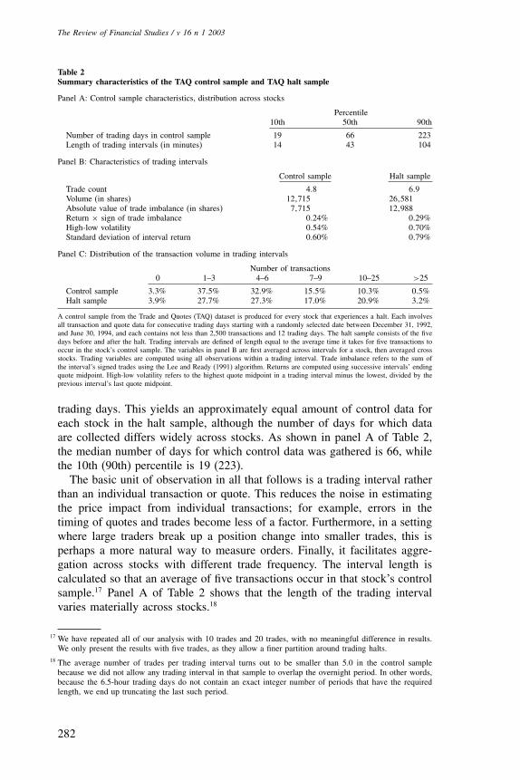
Table 2Summary characteristics of the TAQ control sample and TAQ halt sample
Panel A: Control sample characteristics, distribution across stocks
Percentile10th 50th 90th
Number of trading days in control sample 19 66 223Length of trading intervals (in minutes) 14 43 104
Panel B: Characteristics of trading intervals
Control sample Halt sample
Trade count 4�8 6�9Volume (in shares) 12�715 26�581Absolute value of trade imbalance (in shares) 7�715 12�988Return × sign of trade imbalance 0�24% 0�29%High-low volatility 0�54% 0�70%Standard deviation of interval return 0�60% 0�79%
Panel C: Distribution of the transaction volume in trading intervals
Number of transactions0 1–3 4–6 7–9 10–25 >25
Control sample 3�3% 37�5% 32�9% 15�5% 10�3% 0�5%Halt sample 3�9% 27�7% 27�3% 17�0% 20�9% 3�2%
A control sample from the Trade and Quotes (TAQ) dataset is produced for every stock that experiences a halt. Each involvesall transaction and quote data for consecutive trading days starting with a randomly selected date between December 31, 1992,and June 30, 1994, and each contains not less than 2,500 transactions and 12 trading days. The halt sample consists of the fivedays before and after the halt. Trading intervals are defined of length equal to the average time it takes for five transactions tooccur in the stock’s control sample. The variables in panel B are first averaged across intervals for a stock, then averaged crossstocks. Trading variables are computed using all observations within a trading interval. Trade imbalance refers to the sum ofthe interval’s signed trades using the Lee and Ready (1991) algorithm. Returns are computed using successive intervals’ endingquote midpoint. High-low volatility refers to the highest quote midpoint in a trading interval minus the lowest, divided by theprevious interval’s last quote midpoint.
trading days. This yields an approximately equal amount of control data foreach stock in the halt sample, although the number of days for which dataare collected differs widely across stocks. As shown in panel A of Table 2,the median number of days for which control data was gathered is 66, whilethe 10th (90th) percentile is 19 (223).The basic unit of observation in all that follows is a trading interval rather
than an individual transaction or quote. This reduces the noise in estimatingthe price impact from individual transactions; for example, errors in thetiming of quotes and trades become less of a factor. Furthermore, in a settingwhere large traders break up a position change into smaller trades, this isperhaps a more natural way to measure orders. Finally, it facilitates aggre-gation across stocks with different trade frequency. The interval length iscalculated so that an average of five transactions occur in that stock’s controlsample.17 Panel A of Table 2 shows that the length of the trading intervalvaries materially across stocks.18
17 We have repeated all of our analysis with 10 trades and 20 trades, with no meaningful difference in results.We only present the results with five trades, as they allow a finer partition around trading halts.
18 The average number of trades per trading interval turns out to be smaller than 5.0 in the control samplebecause we did not allow any trading interval in that sample to overlap the overnight period. In other words,because the 6.5-hour trading days do not contain an exact integer number of periods that have the requiredlength, we end up truncating the last such period.
282
Trading Halts in a Specialist Market
The halt sample consists of data for the five trading days before and aftereach halt. We also split these data into trading intervals, using the intervallength calculated in the stock’s control data. These intervals are set so thatthe end (start) of the last (first) interval before (after) the halt coincides withthe start (end) of the halt.For every trading interval in both the control and halt samples, we define
a number of variables used in testing the model. Trade count refers to thenumber of transactions within the trading interval. Share volume refers tothe total number of shares traded within the trading interval. Trade imbalancerefers to the signed share volume over the interval, using a positive (negative)sign for buy (sell) transactions. Both the price change and return variables arecomputed using the last quote midpoint of the current and preceding tradingintervals. The price volatility over a trade interval can be measured using theproduct of return with trade imbalance or using what we refer to as high-low volatility. This latter measure is computed as the difference between thehighest and lowest quote midpoints in the interval divided by the previousinterval’s last quote midpoint.Panel B of Table 2 presents summary statistics of these variables in each of
our two samples. Trading is more active than usual around trading halts, withabout 50% more transactions per interval, a 50% greater trade imbalance, andabout twice the share volume. This evidence is consistent with that providedby Lee, Ready, and Seguin (1994) and by Corwin and Lipson (2000). Panel Cpresents more on the distribution of transaction count within these tradingintervals. The fact that trading interval volatility is only 20–25% higher inthe halt sample than in the control sample is due to the fact that we areincluding trading intervals that are far from trading halts when calculatingthe halt sample averages. Indeed, as we will see later, the volatility close tothe halt is typically much larger than the control sample’s volatility.
4.2 Estimating the specialist’s actionsIn a specialist-organized exchange, the price impact of a transaction is gov-erned by the specialist. Thus we use the statistical precision of price-impactestimates as a proxy for the precision with which the exchange can monitorthe actions of the specialist. To meaningfully compare and pool across stocks,we normalize by using the interval return (rather than price change) and byscaling the interval trade imbalance by the average interval share volume inthe stock’s control sample. We refer to the latter as the scaled trade imbal-ance. Also, all price-impact regressions have an intercept to remove trendsin stock prices.As noted in other studies, the statistical specification of the relation between
signed trades and price changes is nonlinear. For example, Peterson andUmlauf (1994) decompose order imbalance into three terms (the sign, thelevel, and the square) and demonstrate that each is significant, with the firsttwo positive and the third negative. This implies a concave relation between
283

The Review of Financial Studies / v 16 n 1 2003
trade imbalance and price change. Similarly Jones, Kaul, and Lipson (1994)show that the sign of a trade has no less explanatory power than the signedtrade imbalance, again suggesting a concave relation.To facilitate this concave relation we employ a log transformation of the
scaled trade imbalance as the independent variable in our price-impact regres-sions. The transformed trade imbalance is computed as follows. First, wecalculate the logarithm of the absolute value of each interval’s scaled tradeimbalance, and denote this quantity by Lit for stock i in trading interval t.Second, for every interval t and stock i, we compute �Lit −mint Lit ≥ 0,where the minimum is calculated over all trading intervals in the stock’scontrol sample. Third, we sign that excess with the sign of the interval’strade imbalance. We denote the resulting variable by Tit and set it equal tozero if the interval’s trade imbalance is zero. This transformation is centeredon zero and fans out in both the positive and negative direction with logcurvature. It leads to a parsimonious regression,
Rit = �i+�iTit +�it� (10)
where the single parameter, �i, measures the price impact of trades, andwhere the return and transformed trade imbalance for stock i in tradinginterval t are denoted by Rit and Tit , respectively. This regression is esti-mated separately for every stock i = 1� � � � �690 in the control data, over allavailable trading intervals t in the control sample. The estimated coefficient�i measures the incremental return associated with a 10-fold increase in thetrade imbalance (we use base 10 log for this reason). In this simplified modelof the monitoring process, the actions of the specialist are assessed with asingle estimated regression coefficient. The standard error of the estimatedcoefficient is a natural proxy for the imprecision with which the exchangecan assess the specialist.The performance of the log-transformed specification is contrasted with
the performance of a linear specification in Table 3. Not surprisingly, positive(negative) price changes tend to be associated with a positive (negative) tradeimbalance, as reflected by the significantly positive �i coefficients. Both the
Table 3Specification of the statistical assessment of specialists in the control sample
Mean slope (�i) MeanRegressor coefficient t-statistic R2
Scaled trade imbalance 0�0019 8�4 13�2%Log transformed trade imbalance 0�00087 11�5 20�9%
Trading intervals are defined for each stock so that they contain five transactions on average over the control sample (as inTable 2). A trading interval’s return is defined using the last quote midpoint in that and the previous intervals. An interval’strade imbalance is defined as the sum of the interval’s signed trades using the Lee and Ready (1991) algorithm, and an interval’sscaled trade imbalance is defined as its trade imbalance divided by the stock’s average volume per interval (averaged over thestock’s control sample). Two regressions are run, separately for each stock: the return on the scaled trade imbalance, and thereturn on a log transformation of the scaled trade imbalance (as described in Section 4.2). These regressions are run with anintercept (not presented). The table presents the mean statistics across stocks.
284
Trading Halts in a Specialist Market
average regression R2 and the average precision of inferences (i.e., t-statistic)are materially higher with the concave specification.19 In what follows, resultsare presented only using the log-transformed price-impact estimates.
4.3 Testing the model4.3.1 An event study of trading halts. Our model predicts that the infor-mation asymmetry between the exchange and the specialist will tend to beabnormally high around trading halts. Ideally this could be tested by applyingthe technique of the previous section to trading intervals around the halts andassessing whether the uncertainty from those regressions (i.e., the standarderror of the �i estimate) is abnormal versus the control sample. However,there are simply not enough data concentrated around trading halts to runsuch an analysis.An alternative procedure is to use the regression equations estimated in
Section 4.2 from the control sample, focusing on the relative or abnormalprice impact and information asymmetry around the halt.20 Consider a sub-series of K consecutive trading intervals. The price impact over these Kintervals can be written as
Rjt = �i+ �i+�j�Tjt +�jt� t = 1� � � � �K� (11)
where �jt represents the disturbance to the price-impact relation in tradinginterval t for halt j , and �j represents the average price impact deviation(from the control sample �i) that obtains over those K trading intervals.Note that �i and �i are not estimated in this regression; rather they arethe coefficients that were estimated over the stock’s full control sample (inSection 4.2). This specification captures the idea that, in normal conditions,we expect a return of �i +�iTjt in trading interval t, given a transformedtrade imbalance of Tjt . Thus �j represents the average excess price impactcoefficient over the subseries of trading intervals, and the standard error ofthe �j estimate indicates the precision with which that excess can be assessedover those intervals. Implication 1 predicts that this precision is lower whenthe subseries of trading intervals is close to a trading halt than when thesubseries is randomly selected from the control sample.Although our model does not offer any prediction about the size of �j , the
level playing-field hypothesis predicts that liquidity dries up around tradinghalts. As pointed out by Kyle (1985), the effect of trade imbalance on pricesessentially measures the inverse of liquidity. Therefore, to assess both ourmodel and the level playing-field hypothesis, we perform an event study testaround trading halts on both the �j estimates and the standard error of thoseestimates, denoted �j .
19 In results not presented here, multiple regressions adding higher powers of trade imbalance or transformedtrade imbalance did not significantly improve explanatory power.
20 We are grateful to an anonymous referee for suggesting this approach.
285
The Review of Financial Studies / v 16 n 1 2003
We use a simulated empirical distribution for the statistics �j and �j toevaluate whether halt observations are abnormal. For each halt, we randomlyselect 1,000 trading periods from the corresponding stock’s control sample.We then run the regression in Equation (11) over the six consecutive tradingintervals (K = 6) beginning with the selected interval (i.e., six observations,one degree of freedom). This provides an estimate of the coefficient �j andits standard error �j over that subseries of intervals. These 1,000 randomlydrawn estimates are then used to characterize the distribution of �j and �j
under normal circumstances. Note that a separate distribution is estimatedfor each stock.The event study uses the six consecutive trading intervals immediately
preceding the halt and three more sets of six consecutive intervals beforethat. Likewise we consider four subseries after the halt. For each halt, we runthe regression in Equation (11) in each of these halt subseries (again, eachregression has six observations with the unit of observation being a tradinginterval). Finally, the �j and �j estimates are converted to a percentile valueusing the corresponding control-sample empirical distribution.21
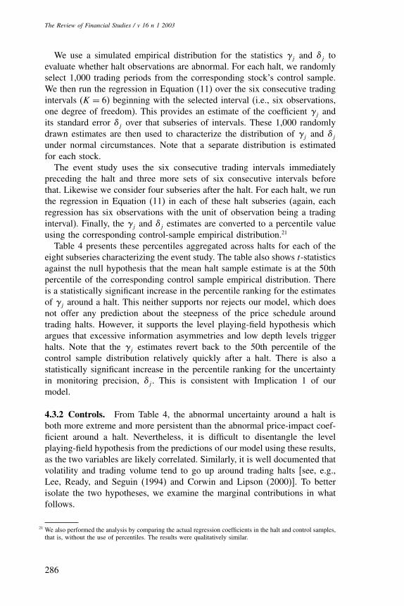
Table 4 presents these percentiles aggregated across halts for each of theeight subseries characterizing the event study. The table also shows t-statisticsagainst the null hypothesis that the mean halt sample estimate is at the 50thpercentile of the corresponding control sample empirical distribution. Thereis a statistically significant increase in the percentile ranking for the estimatesof �j around a halt. This neither supports nor rejects our model, which doesnot offer any prediction about the steepness of the price schedule aroundtrading halts. However, it supports the level playing-field hypothesis whichargues that excessive information asymmetries and low depth levels triggerhalts. Note that the �j estimates revert back to the 50th percentile of thecontrol sample distribution relatively quickly after a halt. There is also astatistically significant increase in the percentile ranking for the uncertaintyin monitoring precision, �j . This is consistent with Implication 1 of ourmodel.
4.3.2 Controls. From Table 4, the abnormal uncertainty around a halt isboth more extreme and more persistent than the abnormal price-impact coef-ficient around a halt. Nevertheless, it is difficult to disentangle the levelplaying-field hypothesis from the predictions of our model using these results,as the two variables are likely correlated. Similarly, it is well documented thatvolatility and trading volume tend to go up around trading halts [see, e.g.,Lee, Ready, and Seguin (1994) and Corwin and Lipson (2000)]. To betterisolate the two hypotheses, we examine the marginal contributions in whatfollows.
21 We also performed the analysis by comparing the actual regression coefficients in the halt and control samples,that is, without the use of percentiles. The results were qualitatively similar.
286

Trading Halts in a Specialist Market
Table 4Event study on the statistical assessment of specialists and the precision of that assessment aroundtrading halts
Subseries before the halt (halt) Subseries after the halt
−4 −3 −2 −1 � 1 2 3 4
� percentile 50�9 51�1 53�2 52�9 60�7 54�1 50�5 50�11�2� 1�5� 4�4� 3�8� 14�1� 5�8� 0�9� 0�2�
� percentile 52�4 51�4 53�1 57�0 74�1 57�7 54�8 52�93�4� 2�3� 5�2� 10�3� 40�1� 13�6� 6�3� 4�1�
Trading intervals are defined for each stock so that they contain five transactions on average over the control sample (as inTable 2). For each halt, subseries of six consecutive trading intervals are used to estimate � in
Rt = �i + �i +��Tt +�t � t = 1� � � � �6�
where �i and �i are the intercept and coefficient estimates from the corresponding stock’s log-transformed trade imbalanceregressions in Table 3. The standard error of the � estimate is denoted �. For each halt, � and � are estimated in each of the foursubseries before a trading halt, and in each of the four subseries after a halt (i.e., the event study spans the 48 trading intervalsaround each halt, since each subseries is six consecutive trading intervals.) We similarly estimate � and � in 1,000 randomlyselected subseries (each containing six consecutive trading intervals) in each stock’s control sample. A percentile value is thenassigned to each of the � and � estimates around a halt using the corresponding distribution of control-sample estimates. Thesepercentile values are then pooled across trading halts, by relative subseries. The table presents the sample mean percentile, anda t-statistic (in parentheses) for the difference between the mean percentile and the 50th percentile.
The volatility and volume controls are structured similarly to the � and �variables. First a control-sample empirical distribution for the volatility (vol-ume) within a subseries of six consecutive trading intervals is constructed.The volatility (volume) over such a subseries is computed as the mean ofthe high-low volatility (trade count) in each of the six trading intervals thatmake up the subseries. The volatility (volume) is similarly calculated overeach of the event subseries and a percentile value determined. The averageof these percentiles, across halts, is presented in Table 5. Both volatility andvolume are unusually large around trading halts. In fact, if anything, thesetwo variables tend to be more abnormal around trading halts than � and �.It is possible that the abnormal increases in � and � in Table 4 arise solely
from their correlation with volatility and trading volume. Such a result would
Table 5Event study on volatility and volume around trading halts
Subseries before the halt (halt) Subseries after the halt
−4 −3 −2 −1 � 1 2 3 4
Volatility 51�8 50�7 52�6 57�1 86�7 71�4 64�5 60�7percentile 2�5� 1�0� 3�4� 9�1� 81�7� 34�6� 22�1� 14�5�
Volume 53�0 53�0 55�2 62�0 91�4 83�0 76�8 73�1percentile 2�4� 2�5� 8�1� 15�3� 97�8� 56�1� 37�6� 31�1�
Trading intervals are defined for each stock so that they contain five transactions on average over the control sample (as inTable 2). Subseries of six consecutive trading intervals are used, as in Table 4, to compute volatility and volume. Volatility isdefined as the average high-low volatility (as in Table 2) over the six trading intervals in the subseries, and volume is definedas the average trade count per interval. For each halt, volatility and volume are estimated in each of the four subseries beforea trading halt, and in each of the four subseries after a halt (i.e., the event study spans the 48 trading intervals around eachhalt, since each subseries is six consecutive trading intervals). Volatility and volume are similarly calculated in 1,000 randomlyselected subseries (each containing six consecutive trading intervals) in each stock’s control sample. A percentile value is thenassigned to each of the volatility and volume computed around a halt using the corresponding distribution of control sampleestimates. These percentile values are then pooled across trading halts, by relative subseries. The table presents the sample meanpercentile, and a t-statistic (in parentheses) for the difference between the mean percentile and the 50th percentile.
287
The Review of Financial Studies / v 16 n 1 2003
say nothing about whether halts are triggered by monitoring uncertainty or byan unlevel playing field. For example, the model does not assert that the costsassociated with monitoring uncertainty are less important when volatility isabnormal. To evaluate whether the incidence of trading halts is consistentwith the model, Table 4 is the relevant analysis. However, confidence in themodel is higher if an effect is detected independently of confounding factors.To this end we increment the analysis performed in Section 4.3.1 with
volatility and volume controls. The controls are constructed by regressingthe 1,000 observations of � and � used to construct their control sampleempirical distributions on the corresponding subseries’ volatility and volume.Thus, for each stock i, we estimate two regressions,22
�it = a�i +b
�i1�it +b
�i2�
2it + c
�i1�it + c
�i2�
2it +�
�it� and (12)
�it = a�i +b�
i1�it +b�i2�
2it + c�i1�it + c�i2�
2it +��
it� (13)
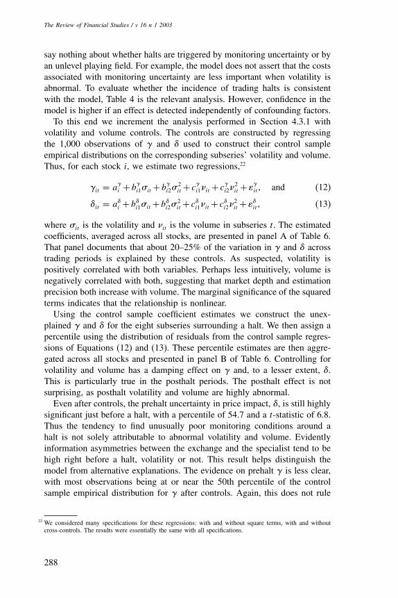
where �it is the volatility and �it is the volume in subseries t. The estimatedcoefficients, averaged across all stocks, are presented in panel A of Table 6.That panel documents that about 20–25% of the variation in � and � acrosstrading periods is explained by these controls. As suspected, volatility ispositively correlated with both variables. Perhaps less intuitively, volume isnegatively correlated with both, suggesting that market depth and estimationprecision both increase with volume. The marginal significance of the squaredterms indicates that the relationship is nonlinear.Using the control sample coefficient estimates we construct the unex-
plained � and � for the eight subseries surrounding a halt. We then assign apercentile using the distribution of residuals from the control sample regres-sions of Equations (12) and (13). These percentile estimates are then aggre-gated across all stocks and presented in panel B of Table 6. Controlling forvolatility and volume has a damping effect on � and, to a lesser extent, �.This is particularly true in the posthalt periods. The posthalt effect is notsurprising, as posthalt volatility and volume are highly abnormal.Even after controls, the prehalt uncertainty in price impact, �, is still highly
significant just before a halt, with a percentile of 54.7 and a t-statistic of 6.8.Thus the tendency to find unusually poor monitoring conditions around ahalt is not solely attributable to abnormal volatility and volume. Evidentlyinformation asymmetries between the exchange and the specialist tend to behigh right before a halt, volatility or not. This result helps distinguish themodel from alternative explanations. The evidence on prehalt � is less clear,with most observations being at or near the 50th percentile of the controlsample empirical distribution for � after controls. Again, this does not rule
22 We considered many specifications for these regressions: with and without square terms, with and withoutcross-controls. The results were essentially the same with all specifications.
288
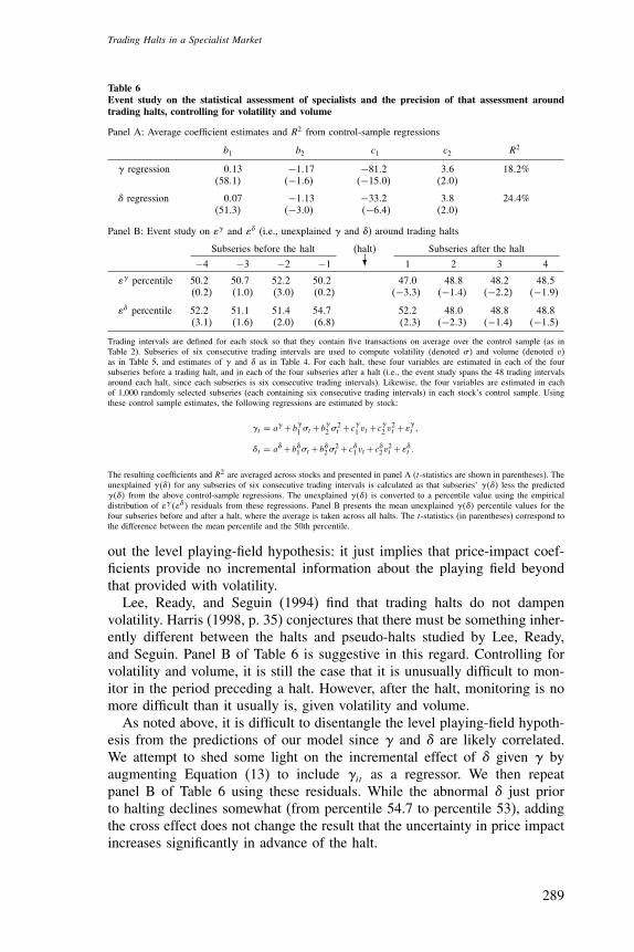
Trading Halts in a Specialist Market
Table 6Event study on the statistical assessment of specialists and the precision of that assessment aroundtrading halts, controlling for volatility and volume
Panel A: Average coefficient estimates and R2 from control-sample regressions
b1 b2 c1 c2 R2
� regression 0�13 −1�17 −81�2 3�6 18�2%58�1� −1�6� −15�0� 2�0�
� regression 0�07 −1�13 −33�2 3�8 24�4%51�3� −3�0� −6�4� 2�0�
Panel B: Event study on �� and �� (i.e., unexplained � and �) around trading halts
Subseries before the halt (halt) Subseries after the halt
−4 −3 −2 −1 � 1 2 3 4
�� percentile 50�2 50�7 52�2 50�2 47�0 48�8 48�2 48�50�2� 1�0� 3�0� 0�2� −3�3� −1�4� −2�2� −1�9�
�� percentile 52�2 51�1 51�4 54�7 52�2 48�0 48�8 48�83�1� 1�6� 2�0� 6�8� 2�3� −2�3� −1�4� −1�5�
Trading intervals are defined for each stock so that they contain five transactions on average over the control sample (as inTable 2). Subseries of six consecutive trading intervals are used to compute volatility (denoted �) and volume (denoted v)as in Table 5, and estimates of � and � as in Table 4. For each halt, these four variables are estimated in each of the foursubseries before a trading halt, and in each of the four subseries after a halt (i.e., the event study spans the 48 trading intervalsaround each halt, since each subseries is six consecutive trading intervals). Likewise, the four variables are estimated in eachof 1,000 randomly selected subseries (each containing six consecutive trading intervals) in each stock’s control sample. Usingthese control sample estimates, the following regressions are estimated by stock:
�t = a� +b�1 �t +b
�2 �
2t + c
�1 vt + c
�2 v
2t +�
�t �
�t = a�+b�1�t +b�2�2t + c�1 vt + c�2 v
2t +��t �
The resulting coefficients and R2 are averaged across stocks and presented in panel A (t-statistics are shown in parentheses). Theunexplained ��� for any subseries of six consecutive trading intervals is calculated as that subseries’ ��� less the predicted��� from the above control-sample regressions. The unexplained ��� is converted to a percentile value using the empiricaldistribution of �� ��� residuals from these regressions. Panel B presents the mean unexplained ��� percentile values for thefour subseries before and after a halt, where the average is taken across all halts. The t-statistics (in parentheses) correspond tothe difference between the mean percentile and the 50th percentile.
out the level playing-field hypothesis: it just implies that price-impact coef-ficients provide no incremental information about the playing field beyondthat provided with volatility.Lee, Ready, and Seguin (1994) find that trading halts do not dampen
volatility. Harris (1998, p. 35) conjectures that there must be something inher-ently different between the halts and pseudo-halts studied by Lee, Ready,and Seguin. Panel B of Table 6 is suggestive in this regard. Controlling forvolatility and volume, it is still the case that it is unusually difficult to mon-itor in the period preceding a halt. However, after the halt, monitoring is nomore difficult than it usually is, given volatility and volume.As noted above, it is difficult to disentangle the level playing-field hypoth-
esis from the predictions of our model since � and � are likely correlated.We attempt to shed some light on the incremental effect of � given � byaugmenting Equation (13) to include �it as a regressor. We then repeatpanel B of Table 6 using these residuals. While the abnormal � just priorto halting declines somewhat (from percentile 54.7 to percentile 53), addingthe cross effect does not change the result that the uncertainty in price impactincreases significantly in advance of the halt.
289

The Review of Financial Studies / v 16 n 1 2003
4.3.3 Types of trading halts. Implication 3 predicts that �j and ��j are
higher around halts called by the exchange than halts called by the specialist.Because news dissemination halts are typically called by the exchange, where-as order imbalance halts are called by the specialists, this partition providesa means to test Implication 3. However, there is another difference betweenthese halt types that tends to obfuscate the analysis. News dissemination haltsare usually triggered by a company official notifying the exchange of corpo-rate matters likely to lead to unusual market conditions. In response, tradingis halted within minutes, even seconds. Conversely, order imbalance haltsare usually preceded by an extended period of unusual order flow and tradedynamics, by definition. This difference in the duration with which “halt-likeconditions” precede the halt itself goes against the predictions of Implica-tion 3: monitoring imprecision several intervals before the halt is more likelywith halts called by specialists.Nevertheless, there is weak support for Implication 3 in Table 7, which
examines the exchange’s ability to monitor the specialist first without andthen with volatility and volume controls (i.e., � as in Table 4, and �� as inpanel B of Table 6). In panel A, without controlling for volatility and volume,monitoring is more difficult at news dissemination halts in the subseriesimmediately preceding the halt, but not in the earlier subseries. However,this difference is not significant. Support is somewhat stronger in panel B,where the difference is statistically significant and begins long before the haltis triggered.
4.3.4 Predicting halts. Our analysis has so far concentrated on whether themonitoring conditions around observed trading halts are consistent with the
Table 7Event study around trading halts by halt types
Panel A: Event study on � around trading halts
Subseries before the halt (halt) Subseries after the halt
−4 −3 −2 −1 � 1 2 3 4
News 49�5 51�2 52�3 57�4 73�7 58�9 53�8 53�5dissemination −0�3� 0�9� 1�6� 5�0� 17�5� 6�5� 2�6� 2�4�
Order 53�4 50�9 52�8 55�6 74�8 57�4 55�5 52�2imbalance 4�1� 1�1� 3�1� 6�5� 34�3� 9�5� 6�7� 2�7�
Panel B: Event study on �� (i.e., unexplained �) around trading halts
Subseries before the halt (halt) Subseries after the halt
−4 −3 −2 −1 � 1 2 3 4
News 53�2 53�8 53�0 56�4 55�7 49�3 49�3 51�4dissemination 2�2� 2�7� 2�1� 4�1� 3�1� −0�4� −0�5� 0�9�
Order 52�3 50�7 51�0 53�8 51�9 47�4 48�7 47�5imbalance 2�6� 0�8� 1�1� 4�4� 1�7� −2�8� −1�5� −2�9�
The analysis for � and �� performed in Table 4 and panel B of Table 6 is repeated separately for the two halt types: newsdissemination halts and order imbalance halts. The figures presented are the percentile values from the corresponding controlsample distribution. The t-statistics, reported in parentheses, test for the difference between the mean percentile and the 50thpercentile.
290
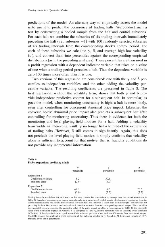
Trading Halts in a Specialist Market
predictions of the model. An alternate way to empirically assess the modelis to use it to predict the occurrence of trading halts. We conduct such atest by constructing a pooled sample from the halt and control subseries.For each halt we combine the subseries of six trading intervals immediatelypreceding the halt (i.e., subseries −1) with 100 randomly selected subseriesof six trading intervals from the corresponding stock’s control period. Foreach of these subseries we calculate �, �, and average high-low volatility(�), and convert them into percentiles against the corresponding empiricaldistributions (as in the preceding analyzes). These percentiles are then used ina probit regression with a dependent indicator variable that takes on a valueof one when a trading period precedes a halt. Thus the dependent variable iszero 100 times more often than it is one.Two versions of this regression are considered: one with the � and � per-
centiles as independent variables, and the other adding the volatility per-centile variable. The resulting coefficients are presented in Table 8. Thefirst regression, without the volatility term, shows that both � and � pro-vide independent predictive content for a subsequent halt. In particular, asgoes the model, when monitoring uncertainty is high, a halt is more likely,even after controlling for concurrent abnormal price impact. Likewise, theconverse holds: abnormal price impact also predicts a subsequent halt aftercontrolling for monitoring uncertainty. Thus there is evidence for both themonitoring and level playing-field motives for a halt. Adding a volatilityterm yields an interesting result: � no longer helps to predict the occurrenceof trading halts. However, � still comes in significantly. Again, this doesnot preclude the level playing-field motive: it simply confirms that volatilityalone is sufficient to account for that motive, that is, liquidity conditions donot provide any incremental information.
Table 8Probit regressions predicting a halt
� � �percentile percentile percentile
Regression 1Coefficient estimate 6�2 30�6Standard error 2�9� 3�0�
Regression 2Coefficient estimate −0�1 19�3 26�5Standard error 3�0� 3�3� 3�3�
Trading intervals are defined for each stock so that they contain five transactions on average over the control sample (as inTable 2). Periods of six consecutive trading intervals make up a subseries. A pooled sample of subseries is constructed from thecontrol sample and the halt sample for each stock. For each halt, one subseries is taken from the halt sample—the subseries justpreceding the halt. One hundred randomly selected subseries are taken from the corresponding control sample. Three variablesare calculated in each subseries: the percentile value of the price impact variable, � (as computed in Table 4), the percentilevalue of the monitoring imprecision variable, � (as computed in Table 4), and the percentile value of volatility, � (as computedin Table 6). A fourth variable is set equal to one if the subseries precedes a halt, and zero if it comes from the control sample.The table presents the results of a probit regression of this indicator variable on �, �, and � . All figures are in units of 10−4.Standard errors are in parentheses.
291
The Review of Financial Studies / v 16 n 1 2003
5. Conclusion
Specialist-organized exchanges bear a principal-agent relationship: theexchange seeks to maximize the overall profits of all specialists, but individualspecialists take the actions that generate those profits. Absent coordination,overall exchange profits are lowered by a negative externality that onespecialist’s pricing schedule imposes on all other specialists. With perfectmonitoring, the exchange can motivate each specialist to quote the overallprofit-maximizing, efficient schedule. However, information asymmetries bet-ween the specialists and the exchange compromise the effectiveness of mon-itoring. Indeed, when those asymmetries are particularly large, the expectedcosts associated with errors in inference on the one hand, versus customergouging on the other hand, can imply negative profits for the exchange.Trading halts allow the exchange to avoid such a situation. Trading haltsalso allow the specialists to avoid situations where their expected individualprofits are negative because of a high likelihood that even diligent actions willbe punished, due to faulty monitoring caused by information asymmetries.Our model of this principal-agent relationship demonstrates the central role
that information asymmetry between the exchange and the specialists playsregarding trading halts. We test the model by constructing an empiricallyobservable proxy for this information asymmetry. Our proxy for monitoringprecision is the statistical precision with which price impact can be esti-mated using transaction level data. In a specialist-organized exchange, theprice impact of transactions is governed by specialists who have a naturalmonopolistic position, so inferences about price impact are de facto infer-ences about the specialist’s actions. We compare this measure around tradinghalts to the same measure in normal circumstances and show that tradinghalts are associated with a substantial decline in the precision of inferencesabout the specialists’ actions.The tests jointly consider the more traditional level playing-field hypoth-
esis, which predicts that informational asymmetries across traders will beunusually large around trading halts. The evidence is consistent with thishypothesis playing a role. However, the level playing-field hypothesis cannotexplain the empirical finding that information asymmetries between the ex-change and the specialists play an independent role. That is, after control-ling for variables associated with the level playing-field hypothesis (volatility,volume, price-impact measures), our proxy for information asymmetry is stillabnormally high around halts. Moreover, it still helps predict a halt.Reputational concerns should be no less important to the profitability of
dealer-organized exchanges, such as the NASDAQ, than they are to the prof-itability of specialist-organized exchanges like the NYSE. As with a specialistmarket, the overall reputation of a dealer market is driven by the actions ofthe individual dealers operating in that market. To the extent that a commonreputational link to the exchange introduces a negative externality across
292
Trading Halts in a Specialist Market
dealers, the principal-agent structure that we model again applies. However,successful gouging of the customer in a dealer market requires the coor-dination of all dealers making a market in the affected stock. Absent suchcoordination, the offending dealer does not gouge the customer, he just takeshimself out of the market. Thus competition across dealers lowers the incen-tive to deviate from the exchange-optimal pricing schedule. Similar com-petition (from the trading crowd) is surely a factor at specialist-organizedexchanges, but it seems plausible that forces of competition act stronger inthe competing dealer arena. Thus proxies for monitoring uncertainty mayplay a weaker role at dealer-market halts than at specialist-market halts.The recent consolidation of specialist firms at the NYSE may be related
to the agency problems considered in this article. When operating indepen-dently, specialists are sometimes tempted to quote privately optimal priceschedules, even though these schedules create negative externalities for theother specialists. In this context, the formation of specialist firms and the con-solidation of existing firms may be a product of the ability of these firms toreduce the frequency and impact of such damaging actions through more effi-cient contracting. Indeed, if the incentives of the specialists operating withina firm are properly realigned, these specialists will avoid actions that reducethe firm’s surplus. The extent to which the consolidation process can helpresolve agency problems on the exchange then depends on the relative abilityof the exchange and of specialist firms to realign their members’ incentives.Finally, our model does not explicitly describe the process by which trading
after a halt is any less susceptible to monitoring problems than trading beforethe halt. It is worth noting, however, that the reopening mechanism is a callauction run by the specialist, who is allowed to participate only so as not to“upset the public balance of supply and demand as reflected by market andlimited price orders.”23 Any trader concerned about poor monitoring con-ditions can avoid agency problems by participating in the reopening callauction. Madhavan and Panchapagesan (2000) find that specialists frequentlyparticipate in daily stock openings, which are subject to the same restriction.However, there is reason to think that the restriction is more binding for areopening following a halt. Daily openings occur 700,000 or so times a year,compared to less than a thousand halts per year. Moreover, halts trigger addi-tional rules on the reopening mechanism, for example, opening indicationsand order imbalances must be posted without change for some time beforethe market can reopen. Thus a halt exposes the specialist to more attentionand scrutiny than that found in the daily opening. We conjecture that thesefactors imply less agency cost on the resumption of trading than existed priorto the halt.Consistent with that conjecture, a substantial number of shares trade in the
reopening auction: 0.98 of the average daily control sample volume for the
23 See rule 104¶2104.11 of the New York Stock Exchange Guide.
293
The Review of Financial Studies / v 16 n 1 2003
halted stock. Moreover, in the spirit of the level playing-field hypothesis,the halt serves as an explicit warning to market participants that monitoringconditions are poor. This can induce caution on the part of liquidity seekers(trading customers) and competitive entry by liquidity providers (the tradingcrowd). Indeed, panel B of Table 6 suggests that, after controlling for theextreme volatility and volume after a halt, abnormal monitoring problems nolonger obtain. The mechanisms for resolution of the poor market conditionsthat triggered the halt in the first place are not well understood and representan area in need of future research.
Appendix A
Proof of Lemma 1. It is straightforward to verify that the expression in Equation (5) is strictlylarger than that in Equation (6) if and only if Equation (7) is satisfied. �
Proof of Lemma 2. Notice that the total expected profits generated by all the specialists of theexchange in a given period (which we denote by �̃e for exchange profits) can be written as
�̃e =N∑i=1
�̃i =N∑i=1
�̃i −
N∑j=1j �=i
�̃ij − ̃i
=
N∑i=1
�̃i −
N∑j=1j �=i
�̃ji − ̃i
≡
N∑i=1
�̃ei �
where the last equality defines the contribution (after negative externalities) of specialist i tothe exchange’s profits. In equilibrium, since all the specialists are identical, they adopt the samestrategy (i.e., they react the same way when they learn p̃i), and so
E[�̃i
]= 1NE[�̃e
]= E[�̃e
i
]� (14)
When specialist i quotes �̃i =G, his expected contribution to the exchange’s profits is
E[�̃e
i ��̃i =G� p̃i
] = E
�̃i −
N∑j=1j �=i
�̃ji − ̃i
∣∣∣∣∣�̃i =G� p̃i
= a−N∑j=1j �=i
0−�
(12− p̃i
)= a−�
(12− p̃i
)� (15)
whereas it is
E[�̃e
i ��̃i = B� p̃i
] = E
�̃i −
N∑j=1j �=i
�̃ji − ̃i
∣∣∣∣∣�̃i = B� p̃i
= 2a− c
N−
N∑j=1j �=i
c
N−�
(12+ p̃i
)= 2a− c−�
(12+ p̃i
)(16)
when he quotes �̃i = B. As shown in Lemma 1, specialist i will quote �̃i = G when p̃i >�2�,
294

Trading Halts in a Specialist Market
and �̃i = B otherwise. Therefore
E[�̃e
i
] = E{E[�̃e
i ��̃i =G� p̃i
]∣∣∣∣p̃i >�
2�
}Pr
{p̃i >
�
2�
}
+E{E[�̃e
i ��̃i = B� p̃i
]∣∣∣∣p̃i ≤�
2�
}Pr
{p̃i ≤
�
2�
}
= a
(1− �
�
)+ 2a− c�
�
�−
(�
4+ �2
2�
)�
This last expression, along with Equation (14), completes the proof. �
Proof of Proposition 1. The exchange and the specialists can only agree to adopt the mon-itoring scheme if the ex ante expected profits of the specialists are increased as a result ofmonitoring with some � > �. Without monitoring, the ex ante expected profits of every spe-cialist are 2a− c [see Equation (2)]; with monitoring, they are given by Equation (8). Thismeans that monitoring is only possible when
a
(1− �
�
)+ 2a− c�
�
�−
(�
4+ �2
2�
)> 2a− c�
which is equivalent to
c−a�
(1− �
�
)− �
4− �2
2�> 0� (17)
For �= 0, this inequality is satisfied for all � ∈ 0�4a� since
c−a�− �
4> c−2a > 0�
This establishes the first part of the proposition. For � ≈ a (i.e., for cN
close to zero), theinequality in Equation (17) becomes
c−a�
(1− a
�
)− �
4− a2
2�> 0�
which can never be satisfied if c is close enough to a. This establishes the second part of theproposition and completes the proof. �
Proof of Lemma 3. Upon learning p̃i, the specialist prefers halting to quoting a conservativeprice schedule if
0> a−(12− p̃i
)⇔ p̃i <
12− a
�� (18)
Similarly the specialist prefers halting to quoting an aggressive price schedule if
0> a+�−(12+ p̃i
)⇔ p̃i >
a+�
�− 1
2� (19)
Halting is preferred to quoting any price schedule when both Equation (18) and Equation (19)are satisfied. For � < 2a+�, this is impossible. For � ∈ �2a+��2a+��, this occurs when
a+�
�− 1
2< p̃i <
12− a
�� (20)
Finally, for �> 2a+��, a+��
− 12< 0 and Equation (19) is always satisfied, so that Equation (20)
reduces to Equation (18). This completes the proof. �
295
The Review of Financial Studies / v 16 n 1 2003
Proof of Lemma 4. We use the same strategy and notation as in the proof of Lemma 2. First,suppose that � ∈ ��2a+��. As shown in Lemma 3, the specialist never halts when � is in thisrange. His decision to quote a conservative or an aggressive price schedule therefore dependson whether Equation (7) is satisfied or not. When the exchange learns p̃i at the beginning ofthe period, it halts whenever it expects the specialist to quote an aggressive price schedule (i.e.,when p̃i ≤ �
2�), and then �̃e
i = 0. Thus, for this range of �, we can use Equations (15) and (16)to get
E[�̃e
i
] = E{E[�̃e
i ��̃i =G� p̃i
]∣∣∣∣p̃i >�
2��no halt
}Pr
{p̃i >
�
2�� no halt
}
+E{E[�̃e
i ��̃i = B� p̃i
]∣∣∣∣p̃i ≤�
2�� no halt
}Pr
{p̃i ≤
�
2�� no halt
}
= E{a−�
(12− p̃i
)∣∣∣∣p̃i >�
2�
}Pr
{p̃i >
�
2�
}
+E{2a− c−�
(12+ p̃i
)∣∣∣∣p̃i ≤�
2�
}1−q�Pr
{p̃i ≤
�
2�
}
=∫ 1
2
�2�
[a−�
(12−p
)]2dp+ 1−q�
∫ �2�
0
[2a− c−�
(12+p
)]2dp
= a
(1− �
�
)−�
(14− �
2�+ �2
4�2
)+ 1−q�2a− c�
�
�− 1−q��
(14+ �2
2�2
)�
This expression yields the first line of Equation (9). Now suppose that � ∈ �2a+��2a+��.Lemmas 1 and 3 tell us that the specialist, when the exchange does not halt, will quote anaggressive price schedule for p̃i ∈ �0� a+�
�− 1
2, will halt for p̃i ∈ a+�
�− 1
2� 1
2− a
��, and will
quote a conservative price schedule for p̃i ∈ � 12− a
�� 1
2. When the exchange does observe p̃i, it
calls a halt for p̃i ∈ �0� a+��
− 12. Thus
E[�̃e
i
] = E{E[�̃e
i ��̃i =G� p̃i
]∣∣∣∣p̃i >�
2�� no halt
}Pr
{p̃i >
�
2�� no halt
}
+E{E[�̃e
i ��̃i = B� p̃i
]∣∣∣∣p̃i ≤�
2�� no halt
}Pr
{p̃i ≤
�
2�� no halt
}
= E{a−�
(12− p̃i
)∣∣∣∣p̃i >12− a
�
}Pr
{p̃i >
12− a
�
}
+E{2a− c−�
(12+ p̃i
)∣∣∣∣p̃i ≤a+�
�− 1
2
}1−q�Pr
{p̃i ≤
a+�
�− 1
2
}
=∫ 1
2
12 − a
�
[a−�
(12−p
)]2dp+ 1−q�
∫ a+�� − 1
2
0
[2a− c−�
(12+p
)]2dp
= 2a2
�−�
a2
�2+ 1−q�2a− c�
[2a+��
�−1
]− 1−q�
[(a+�
�
)2
− 14
]�
which yields the second line of Equation (9). Finally, suppose that � ∈ 2a+�����. In thiscase, Lemmas 1 and 3 imply that the specialist never quotes an aggressive price schedule, sothat the exchange never halts trading. The specialist quotes a conservative price schedule when
296
Trading Halts in a Specialist Market
p̃i >12− a
�and halts otherwise. We then have
E[�̃e
i
] = E{E[�̃e
i ��̃i =G� p̃i
]∣∣∣∣p̃i >�
2�� no halt
}Pr
{p̃i >
�
2�� no halt
}
+E{E[�̃e
i ��̃i = B� p̃i
]∣∣∣∣p̃i ≤�
2�� no halt
}Pr
{p̃i ≤
�
2�� no halt
}
= E{a−�
(12− p̃i
)∣∣∣∣p̃i >12− a
�
}Pr
{p̃i >
12− a
�
}+0
=∫ 1
2
12 − a
�
[a−�
(12−p
)]2dp = 2a2
�−�
a2
�2= a2
��
and this yields the third line of Equation (9). �
Proof of Proposition 2. To prove this result, we need to show that the expression for E��̃i inLemma 4 is larger than that in Lemma 2 for any � > �. First, suppose that � ∈ ��2a+��. Thedifference between the two expressions is then
[a
(1− �
�
)+ 1−q�2a− c�
�
�− �
4− �2
2�+q
�
2
(1+ �
2�
)]
−[a
(1− �
�
)+ 2a− c�
�
�− �
4− �2
2�
]= qc−2a�+q
�
2
(1+ �
2�
)> 0�
Now suppose that � ∈ �2a+��2a+��. The difference is now
2a2
�+
≤1︷ ︸︸ ︷1−q�
<0︷ ︸︸ ︷2a− c�
≥0︷ ︸︸ ︷[2a+��
�−1
]−a2
�− 1−q�
[a+��2
�− �
4
]
−{a
(1− �
�
)+ 2a− c�
�
�− �
4− �2
2�
}
≥
2a2
�+ 2a− c�
[2a+��
�−1
]− a2
�−
[a+��2
�− �
4
]+q�
≥0︷ ︸︸ ︷[(a+�
�
)2
− �
4
]
−{a
(1− �
�
)+ 2a− c�
�
�− �
4− �2
2�
}
≥ a2
�+
<0︷ ︸︸ ︷2a− c�
≤0︷ ︸︸ ︷[2a+�
�−1
]−a2 +2a�+�2
�+ �
2−a+ a�
�+ �2
2�
≥ 1�
−a�− �2
2+
≥ �2 2a+��︷︸︸︷�2
2−a�
≥ 1
�
−a�− �2
2+
≥�2a+��︷︸︸︷��
≥ �
2�2a+�� > 0�
297

The Review of Financial Studies / v 16 n 1 2003
Finally, suppose that � ∈ 2a+�����. In this case, the difference is
a2
�−
a(1− �
�
)+
<0︷ ︸︸ ︷2a− c�
�
�− �
4− �2
2�
>
a2
�−a+
>0︷︸︸︷a�
�+�
4+
>0︷︸︸︷�2
2�
>1�
(a− �
2
)2
> 0�
This completes the proof. �
Proof of Proposition 3. We need to find a � > � such that E��̃i in Lemma 4 is greater than2a− c. Take �= 2a+��. Then, using Equation (9), we have
E[�̃i
]= a2
2a+��> 0> 2a− c�
�
Proof of Proposition 4. We need to show that E�p̃i � halt < 14= E�p̃i. For � ∈ ��2a+��,
this is trivial, since halts are only called by the exchange when p̃i ∈ �0� �2� ⊂ �0� 1
2. This
is also trivial for � ∈ 2a+�����, since halts are then only called by the specialist whenp̃i ∈ �0� 1
2− a
�⊂ �0� 1
2. So it only remains to show that this is true for � ∈ �2a+��2a+��.
In that case,
E�p̃i�halt
= qE�p̃i�p̃i≤ 12− a
�Pr�p̃i≤ 1
2− a
��+1−q�E�p̃i� a+�
�<p̃i≤ 1
2− a
�Pr� a+�
�− 1
2<p̃i≤ 1
2− a
��
q Pr�p̃i≤ 12− a
��+1−q�Pr� a+�
�− 1
2<p̃i≤ 1
2− a
��
=q∫ 1
2 − a�
0 2pdp+1−q�∫ 1
2 − a�
a+�� − 1
22pdp
q(1− 2a
�
)+1−q�
(1− 2a
�− 2a+��
�+1
)
=q(
12− a
�
)2+1−q�
[(12− a
�
)2−(
a+��
− 12
)2]
q(1− 2a
�
)+1−q�2
(1− 2a+�
�
)= 1
4q�−2a�2+1−q�4��−2a−��
q��−2a�+1−q�2��−2a−���
This last quantity will be smaller than 14if and only if
q�−2a�2 + 1−q�4��−2a−�� < q��−2a�+ 1−q�2��−2a−���
Since this inequality is linear in q, it is sufficient to verify that it holds for q = 0 and q = 1.For q = 0, we need to verify that � > 2�, which is true since � > 2a+� > 2�+� > 2�. Forq = 1, we need to verify that �−2a < �, which is obviously true. This completes the proof. �
Proof of Proposition 5. This result only applies to values of � ∈ �2a+��2a+��, since thisis the only range in which halts can be called by either the exchange or the specialist. In thatrange, the exchange calls a halt when p̃i ∈ �0� a+�
�− 1
2, whereas the specialist calls one when
p̃i ∈ a+��
− 12� 1
2− a
��. The result easily follows. �
298

Trading Halts in a Specialist Market
ReferencesBaumol, W. J., 1972, “On Taxation and the Control of Externalities,” American Economic Review, 62, 307–322.
Benveniste, L. M., A. J. Marcus, and W. J. Wilhelm, 1992, “What’s Special About the Specialist?,” Journalof Financial Economics, 32, 61–86.
Bhattacharya, U., and M. Spiegel, 1991, “Insiders, Outsiders, and Market Breakdowns,” Review of FinancialStudies, 4, 255–282.
Bhattacharya, U., and M. Spiegel, 1998, “Anatomy of a Market Failure: NYSE Trading Suspensions(1974–1988),” Journal of Business and Economic Statistics, 16, 216–226.
Blume, M. E., and M. A. Goldstein, 1997, “Quotes, Order Flow, and Price Discovery,” Journal of Finance,52, 221–244.
Buchanan, J. M., 1969, “External Diseconomies, Corrective Taxes, and Market Structure,” American EconomicReview, 59, 174–177.
Corwin, S. A., 2002, “Specialist Performance and New Listing Allocations on the NYSE: An EmpiricalAnalysis,” working paper, University of Notre Dame.
Corwin, S. A., and M. L. Lipson, 2000, “Order Flow and Liquidity Around NYSE Trading Halts,” Journalof Finance, 55, 1771–1805.
DeMarzo, P. M., M. J. Fishman, and K. M. Hagerty, 2000, “The Enforcement Policy of a Self-RegulatoryOrganization,” working paper, Stanford University.
Fischel, D. R., 1986, “Regulatory Conflict and Entry Regulation of New Futures Contracts,” Journal ofBusiness, 59, S85–S102.
Fischel, D. R., and S. J. Grossman, 1984, “Customer Protection in Futures and Securities Markets,” Journalof Futures Markets, 4, 273–295.
Greenwald, B. C., and J. C. Stein, 1991, “Transactional Risk, Market Crashes, and the Role of CircuitBreakers,” Journal of Business, 64, 443–462.
Grossman, S. J., 1990, “Institutional Investing and New Trading Technologies,” in Market Volatility andInvestor Confidence, New York Stock Exchange.
Groves, T., 1973, “Incentives in Teams,” Econometrica, 41, 617–631.
Harris, L. E., 1998, “Circuit Breakers and Program Trading Limits: The Lessons Learned,” in Robert E. Litanand Anthony M. Santomero (eds.), Papers on Financial Services, Brookings Institution Press, Washington,DC.
Holmstrom, B., 1982, “Moral Hazard in Teams,” Bell Journal of Economics, 13, 324–340.
Hopewell, M. H., and A. L. Schwartz Jr., 1978, “Temporary Trading Suspensions in Individual NYSE Secu-rities,” Journal of Finance, 33, 1355–1373.
Jones, C. M., G. Kaul, and M. L. Lipson, 1994, “Information, Trading, and Volatility,” Journal of FinancialEconomics, 36, 127–154.
Kandel, E., and E. P. Lazear, 1992, “Peer Pressure and Partnerships,” Journal of Political Economy, 100,801–817.
King, R., G. Pownall, and G. Waymire, 1992, “Corporate Disclosure and Price Discovery Associated withNYSE Temporary Trading Halts,” Contemporary Accounting Research, 8, 509–531.
Kodres, L. E., and D. P. O’Brien, 1994, “The Existence of Pareto-Superior Limits,” American EconomicReview, 84, 919–932.
Kryzanowski, L., 1979, “The Efficacy of Trading Suspensions: A Regulatory Action Designed to Prevent theExploitation of Monopoly Information,” Journal of Finance, 34, 1187–1200.
299

The Review of Financial Studies / v 16 n 1 2003
Kumar, P., and D. J. Seppi, 1994, “Information and Index Arbitrage,” Journal of Business, 67, 481–509.
Kyle, A. S., 1985, “Continuous Auctions and Insider Trading,” Econometrica, 53, 1315–1335.
Kyle, A. S., 1988, “Trading Halts and Price Limits,” Review of Futures Markets, 7, 426–434.
Lee, C. M. C., and M. J. Ready, 1991, “Inferring Trade Direction from Intraday Data,” Journal of Finance,46, 733–746.
Lee, C. M. C., M. J. Ready, and P. J. Seguin, 1994, “Volume, Volatility, and New York Stock ExchangeTrading Halts,” Journal of Finance, 49, 183–214.
Madhavan, A., and V. Panchapagesan, 2000, “Price Discovery in Auction Markets: A Look Inside the BlackBox,” Review of Financial Studies, 13, 627–658.
Mahoney, P. G., 1997, “The Exchange as a Regulator,” Virginia Law Review, 83, 1453–1500.
Miller, M. H., 1991, Financial Innovations and Market Volatility, Blackwell, Cambridge, MA.
New York Stock Exchange, 2001, New York Stock Exchange Guide, Volume 2: Constitution and Rules,Commerce Clearing House, Inc., Chicago, IL.
Petersen, M. A., and S. Umlauf, 1994, “Quote Revisions and the Quoted Size: An Empirical Analysis,”working paper, Northwestern University.
Pigou, A. C., 1932, The Economics of Welfare (4th ed.), MacMillan, London.
Pirrong, S. C., 1995, “The Self-Regulation of Commodity Exchanges: The Case of Market Manipulation,”Journal of Law and Economics, 38, 141–206.
Spiegel, M., and A. Subrahmanyam, 2000, “Asymmetric Information and News Disclosure Rules,” Journal ofFinancial Intermediation, 9, 363–403.
Subrahmanyam, A., 1994, “Circuit Breakers and Market Volatility: A Theoretical Perspective,” Journal ofFinance, 49, 237–254.
Subrahmanyam, A., 1995, “On Rules Versus Discretion in Procedures to Halt Trade,” Journal of Economicsand Business, 47, 1–16.
Wu, L., 1998, “Market Reactions to the Hong Kong Trading Suspensions: Mandatory Versus Voluntary,”Journal of Business Finance and Accounting, 25, 419–437.
300