the role of initial geometry in experimental models of ... · wound healing assays are initiated by...

The role of initial geometry in experimental

models of wound closing

Wang Jin1, Kai-Yin Lo2, Shih–En Chou2, Scott W McCue1

∗Matthew J Simpson1

1 School of Mathematical Sciences, Queensland University of Technology (QUT)

Brisbane, Queensland 4000, Australia.

2 Department of Agricultural Chemistry, National Taiwan University

Taipei 10617, Taiwan.

Abstract

Wound healing assays are commonly used to study how populations of cells, ini-

tialised on a two-dimensional surface, act to close an artificial wound space. While

real wounds have different shapes, standard wound healing assays often deal with

just one simple wound shape, and it is unclear whether varying the wound shape

might impact how we interpret results from these experiments. In this work, we

describe a new kind of wound healing assay, called a sticker assay, that allows us

to examine the role of wound shape in a series of wound healing assays performed

with fibroblast cells. In particular, we show how to use the sticker assay to exam-

ine wound healing with square, circular and triangular shaped wounds. We take a

standard approach and report measurements of the size of the wound as a function

of time. This shows that the rate of wound closure depends on the initial wound

shape. This result is interesting because the only aspect of the assay that we change

is the initial wound shape, and the reason for the different rate of wound closure

is unclear. To provide more insight into the experimental observations we describe

our results quantitatively by calibrating a mathematical model, describing the rel-

evant transport phenomena, to match our experimental data. Overall, our results

Preprint submitted to Elsevier 12 March 2018

arX

iv:1

711.

0716

2v1

[q-

bio.

CB

] 2

0 N

ov 2

017

suggest that the rates of cell motility and cell proliferation from different initial

wound shapes are approximately the same, implying that the differences we observe

in the wound closure rate are consistent with a fairly typical mathematical model

of wound healing. Our results imply that parameter estimates obtained from an ex-

periment performed with one particular wound shape could be used to describe an

experiment performed with a different shape. This fundamental result is important

because this assumption is often invoked, but never tested.

Key words: Wound healing assay; Sticker assay; Wound shape; Transport process

∗ Corresponding author

Email address: [email protected], Telephone + 617 31385241,

Fax + 617 3138 2310 (∗Matthew J Simpson1).

2

1 Introduction

Two–dimensional in vitro cell migration assays are routinely used to study

wound healing and cancer cell spreading. In these assays, both cell migration

and cell proliferation play a key role at the phenotypic level (Keese et al., 2004;

Singh et al., 2003). Generally there are two types of cell migration assays: (i)

Proliferation assays are initiated by placing cells as a uniform monolayer,

at low density, onto a two-dimensional surface (Jones et al., 2001); and (ii)

Wound healing assays are initiated by creating an artificial wound in a uni-

formly distributed monolayer of cells (Kramer et al., 2013). In a proliferation

assay, individual cells undergo both migration and proliferation events, which

increases the cell density in the spatially uniform monolayer of cells (Jones et

al., 2001). In contrast, wound healing assays involve individual cells moving

into the initially vacant wound area. The effects of cell migration and cell pro-

liferation, combined, lead to the eventual closure of the wound space (Kramer

et al., 2013).

Various types of wound healing assays are reported in the literature (Ariano

et al., 2011; Ascione et al., 2017; Cai et al., 2007; Gough et al., 2011; Keese et

al., 2004; Lee et al., 2010; Sheardown and Chent, 1996; Treloar et al., 2013).

Despite the fact that real wounds can take on arbitrary shapes and sizes, the

most common wound shapes used in in vitro wound healing assays are a simple

long thin rectangular wound or a circular wound (Keese et al., 2004; Riahi et

al., 2012; Tremel et al., 2009; van der Meer et al., 2010; Yarrow et al., 2004)

and the question of whether the initial wound shape plays an important role

is often overlooked (see Table 1). We note that Madison and Gronwall (1992)

compare the rate of healing for circular and square skin wounds on the dorsum

of the metacarpus of horses, and they suggest that the rate of wound healing

is not affected by the initial wound shape. However, more recent quantitative

analysis of several in vitro models of wound healing suggest that the rate of

3

wound healing can be extremely sensitive to the initial configuration of cells

(Jin et al., 2016, Treloar et al., 2014). Therefore, it is of interest to develop

a new in vitro assay which can be used to study wound healing for a variety

of wound shapes, and to analyze results from the new experiments using a

mathematical model to provide quantitative insight into the role of initial

wound shape.

4

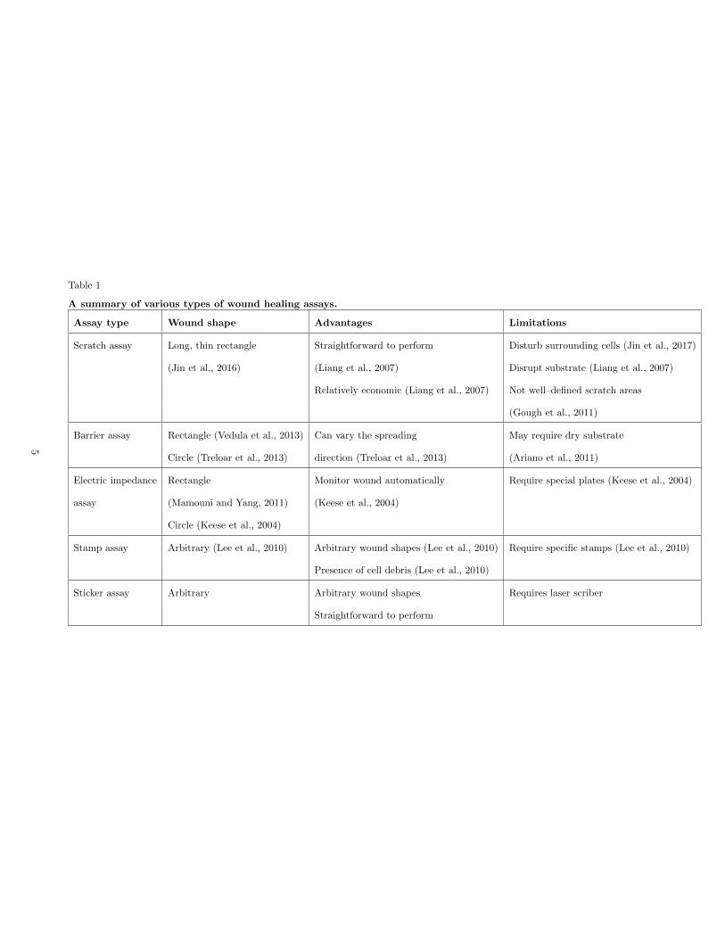
Table 1

A summary of various types of wound healing assays.

Assay type Wound shape Advantages Limitations

Scratch assay Long, thin rectangle Straightforward to perform Disturb surrounding cells (Jin et al., 2017)

(Jin et al., 2016) (Liang et al., 2007) Disrupt substrate (Liang et al., 2007)

Relatively economic (Liang et al., 2007) Not well–defined scratch areas

(Gough et al., 2011)

Barrier assay Rectangle (Vedula et al., 2013) Can vary the spreading May require dry substrate

Circle (Treloar et al., 2013) direction (Treloar et al., 2013) (Ariano et al., 2011)

Electric impedance Rectangle Monitor wound automatically Require special plates (Keese et al., 2004)

assay (Mamouni and Yang, 2011) (Keese et al., 2004)

Circle (Keese et al., 2004)

Stamp assay Arbitrary (Lee et al., 2010) Arbitrary wound shapes (Lee et al., 2010) Require specific stamps (Lee et al., 2010)

Presence of cell debris (Lee et al., 2010)

Sticker assay Arbitrary Arbitrary wound shapes Requires laser scriber

Straightforward to perform

5

Experimental data from in vitro wound healing assays are commonly presented

by plotting the time evolution of wound area as the experiment proceeds and

the wound closes (Bachstetter et al., 2016; Johnston et al., 2015; Ueck et al.,

2017; Yarrow et al., 2004). While some studies report the time evolution of

the exact wound area (Leu et al., 2012; Ueck et al., 2017; Yarrow et al., 2004),

others studies report results in a non-dimensional format by reporting the

wound area relative to the initial wound area (Ascione et al., 2017; Bachstetter

et al., 2016; Johnston et al., 2015; Katakowski et al., 2017; Walter et al., 2010).

Although both types of measurements provide an indication of the speed at

which wound healing takes place, reporting the data in terms of the relative

wound area does not provide any information about the role of initial wound

shape or initial wound size. Therefore, when comparing wound healing assays

with different initial wound shapes, we believe it is important to report the

data in terms of the wound area because this explicitly accounts for differences

in the initial condition instead of simply reporting the area data relative to

the initial wound area.

Many different types of mathematical and computational models have been

used to mimic in vitro collective cell migration assays. One approach is to use

a discrete random walk model (Codling et al. 2008). In some random walk

models, cell migration is represented by an unbiased, nearest-neighbour exclu-

sion process, in which cell-to-cell crowding is modelled by hard core exclusion

(Painter and Hillen, 2002; Simpson et al., 2010). Cell proliferation can be

modelled by allowing individual agents in the simulation to divide to produce

daughter agents (Simpson et al., 2010). Crowding effects can be incorporated

into the proliferation mechanism by randomly choosing a nearest neighbour

lattice site for the placement of the daughter agent, and only allowing the pro-

liferation event to succeed if the target site is vacant (Simpson et al., 2010).

While discrete random walk models provide information relevant to individ-

ual cells within the population, it is also possible to describe the behaviour

6

of the population of cells by considering the continuum-limit description of

the random walk model, which in this case, gives rise to a two-dimensional

reaction diffusion partial differential equation (PDE) that is equivalent to the

two-dimensional Fisher-Kolmogorov model (Fisher, 1937; Kolmogorov et al.

1937). This connection with the Fisher-Kolmogorov model is of interest be-

cause this model, and many other generalisations of this model, have been

used previously to study collective cell migration problems, including wound

healing type assays (e.g. Maini et al., 2004a, 2004b; Painter and Sherratt,

2003; Sengers et al., 2007; Sherratt and Murray, 1990; Swanson et al., 2003;

Swanson, 2008).

In this study we develop and describe a novel experimental approach to in-

vestigate the role of initial wound shape. We perform sticker assays using

fibroblast cells and three different initial wound shapes: squares, circles, and

equilateral triangles. In addition to describing our new experimental protocol,

and experimental results, we attempt to quantify the mechanisms that drive

the wound healing process by calibrating the solution of a mathematical model

to match the experimental data. To estimate the rate of cell proliferation and

the carrying capacity density, we examine a series of proliferation assays and

apply the continuum-limit description of the random walk model to match the

experimental data. To estimate the cell diffusivity we use the discrete random

walk model to mimic a series of sticker assays with different shaped wounds.

Comparing the snapshots from discrete simulations to the experimental im-

ages allows us to choose the cell diffusivity so that the discrete model matches

the experimental images in terms of the position of the leading edge of the

population of cells. Overall, our results indicate that the parameters obtained

from different wound shapes are approximately constant, suggesting that the

initial wound geometry has no identifiable impact on the key mechanisms of

cell motility and cell proliferation. This is an important outcome because it is

common to perform a wound healing assay with one particular geometry and

7

to simply assume that the results might apply to another geometry, and this

standard assumption is rarely considered or tested. Furthermore, this result is

important because our experimental data, alone, shows that the rate of wound

closure depends on the initial shape of the wound.

Overall, while we find that different initial wound shapes lead to different

rates of wound closure, our careful calibration of a mathematical model to

the experimental data confirms that the differences in observed wound closure

rates are entirely consistent with the underlying transport phenomena that

drives wound healing. In particular, we find that the rates of cell migration

and cell proliferation are unaffected by the initial wound shape.

2 Methods

2.1 Experimental methods

The new experimental protocol for the sticker assay is shown schematically

in Figure 1. We perform the experiments with NIH 3T3 fibroblast cell line

purchased from the Bioresource Collection and Research Center (BCRC), Tai-

wan. A complete medium composed of Dulbecco’s Modified Eagle’s medium

(DMEM, Gibco, USA) and 10% calf serum (CS, Invitrogen, USA) is used for

cell culture. Cells are incubated in tissue culture polystyrene (TCPS) flasks

(Corning, USA) in 5% CO2 at 37 ◦C, and grown to approximately 90% con-

fluence before each passage.

The wound shapes are drawn in AutoCAD (Autodesk, USA) and then loaded

into a CO2 laser scriber (ILS2, Laser Tools & Technics Corp., Taiwan), to

ablate desired wound shapes on a double-sided sticker (8018, 3M, USA). Three

different types of wound shapes are designed in this experiment: square, circle,

and equilateral triangle. The side length of each square and triangle sticker

8

is 2 mm, and the diameter of each circle sticker is also 2 mm. The sticker

is folded to form a handle, and is attached to the centre of a dish, with a

diameter 35 mm. The dish is exposed to UV for 30 minutes for sterilisation. 3

× 105 cells are placed, as uniformly as possible, into the dish, and incubated

overnight. To initiate the wound healing assay, the sticker is removed to reveal

the cell-free wound area. The plates are continually incubated in 5% CO2 at

37 ◦C. The distribution of cells is imaged at t = 0, 9, 24, 33, 48, 57, 72 h for

the assays initiated with the square and circular wound shapes. The assays

initiated with the triangular wounds are imaged at t = 0, 9, 24, 33, 48, 57

h. For each wound shape we perform three identically prepared experimental

replicates (n = 3).

A proliferation assay is initiated in the same way as the wound healing assay

except that there is no wound. The plates are continually incubated in 5%

CO2 at 37 ◦C and images are recorded at t = 0, 9, 24, 33, 48, 57, 72, 81,

96 h. We perform one experimental replicate of the proliferation assay and

analyse data from this assay by estimating the cell density in three different,

identically–sized, rectangular subregions within the population (Johnston et

al., 2015).

9

35 mm(a) (b)

(e) (f)

(d)

(g)

t = 0 h t = 48 h

Cells

Handle

Foot

(c)

Fig. 1. Sticker assay protocol. (a) Stickers for creating square, circular, and triangular wound shapes. The side length and the diameter

of square, equilateral triangle, and circular stickers are 2 mm. The red region shows both the foot of the sticker and the handle. The

dashed line indicates where the sticker is folded to create the handle so that the foot of the sticker can be easily attached, and removed

from the tissue culture plate. (b) Corning R© cell culture dish. (c) Isometric schematic of a 35 mm diameter cell culture plate showing

the sticker attached to the plate before the cells are seeded into the dish. (d) Isometric schematic of the cell culture plate showing the

apparatus after the cells are seeded into the dish. (e) Top view of the experiment prior to the sticker being lifted. The blue dashed area

shows the field of view that is imaged. (f) Experimental field of view at t = 0 h with a square wound shape. (g) Experimental field of

view at t = 48 h showing the progression of the assay. The scale bar corresponds to 500 µm.10

2.2 Edge detection method

We use ImageJ (Ferreira and Rasband, 2012) to detect the edges of the wound

area in both the experimental and the simulation images (Treloar et al., 2013).

For all images, the scale is first set using the Set Scale function. We find that

932 pixels corresponds to 1 mm for all experimental images, and 304 pixels

corresponds to 1 mm for all the simulation images. For each experimental

image the contrast is enhanced by increasing the contrast and decreasing the

brightness (Image–Adjust–Brightness/Contrast). The edges of the cells are

then detected (Plugins–Canny Edge Detector), and enhanced using the Sobel

method (Process–Find Edges). Depending on the quality of the experimental

image, the Find Edges function may need to be used several times, both locally

and globally for the edge of the wound area to be successfully detected. The

edge of the wound area is automatically detected using the wand tracing tool.

Then the wound area is calculated (Analyze–Measure). For each simulation

image, the colour image is first set to grayscale (Image–Type–32-bit). Then

the edges of cells are detected (Plugins–Canny Edge Detector), and enhanced

using the Sobel method (Process–Find Edges) two to three times. The wound

area is automatically detected using the wand tracing tool and calculated

(Analyze–Measure). An important feature of our method is that we use the

exact same image processing tools to quantify the time evolution of the area

of the wound in both the experimental and the simulation images (Treloar et

al., 2014).

2.3 Mathematical methods

2.3.1 Discrete model

We use a discrete random walk model, in which each agent represents a single

cell, to simulate the experiments. Simulations are performed on a hexagonal

11

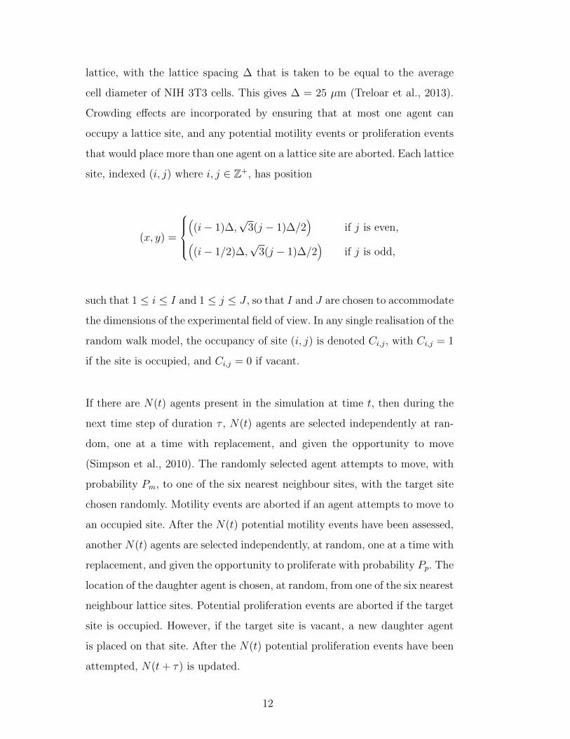
lattice, with the lattice spacing ∆ that is taken to be equal to the average

cell diameter of NIH 3T3 cells. This gives ∆ = 25 µm (Treloar et al., 2013).

Crowding effects are incorporated by ensuring that at most one agent can

occupy a lattice site, and any potential motility events or proliferation events

that would place more than one agent on a lattice site are aborted. Each lattice

site, indexed (i, j) where i, j ∈ Z+, has position

(x, y) =

((i− 1)∆,

√3(j − 1)∆/2

)if j is even,

((i− 1/2)∆,

√3(j − 1)∆/2

)if j is odd,

such that 1 ≤ i ≤ I and 1 ≤ j ≤ J , so that I and J are chosen to accommodate

the dimensions of the experimental field of view. In any single realisation of the

random walk model, the occupancy of site (i, j) is denoted Ci,j, with Ci,j = 1

if the site is occupied, and Ci,j = 0 if vacant.

If there are N(t) agents present in the simulation at time t, then during the

next time step of duration τ , N(t) agents are selected independently at ran-

dom, one at a time with replacement, and given the opportunity to move

(Simpson et al., 2010). The randomly selected agent attempts to move, with

probability Pm, to one of the six nearest neighbour sites, with the target site

chosen randomly. Motility events are aborted if an agent attempts to move to

an occupied site. After the N(t) potential motility events have been assessed,

another N(t) agents are selected independently, at random, one at a time with

replacement, and given the opportunity to proliferate with probability Pp. The

location of the daughter agent is chosen, at random, from one of the six nearest

neighbour lattice sites. Potential proliferation events are aborted if the target

site is occupied. However, if the target site is vacant, a new daughter agent

is placed on that site. After the N(t) potential proliferation events have been

attempted, N(t+ τ) is updated.

12

2.3.2 Continuum limit of the discrete model

While discrete models are useful to mimic and predict experimental observa-

tions, it is difficult to obtain more general insight using this approach. There-

fore, it is relevant to consider a mean field continuum limit description because

we can then use additional mathematical and computational methods to gain

insight into the model (O’Dea and King, 2012). The mean field continuum

limit description of the random walk model can be derived by formulating an

approximate discrete conservation statement describing the change in aver-

age occupancy of site s = (i, j) during the interval from time t to time t + τ

(Simpson et al., 2010)

δ〈Cs〉 = +

change in occupancy due to migration into site s︷︸︸︷Pm6

(1− 〈Cs〉)∑

s′∈N{s}〈Cs′〉

−

change in occupancy due to migration out of site s︷︸︸︷Pm6〈Cs〉

∑

s′∈N{s}(1− 〈Cs′〉)

+

change in occupancy due to proliferation into site s︷︸︸︷Pp6

(1− 〈Cs〉)∑

s′∈N{s}〈Cs′〉 , (1)

where 〈Cs〉 ∈ [0, 1] is the average occupancy of site s, where the average

is obtained by averaging the occupancy over a large number of identically

prepared realisations, N{s} is the set of six nearest-neighbour sites around

site s, and∑

s′∈N{s}〈Cs′〉 is the sum of the average occupancy of the nearest

neighbour sites. To proceed we invoke the usual mean field assumption which

amounts to treating the average occupancy of lattice sites as independent

(Simpson et al., 2010).

We then use Taylor series to expand each term in Eq. (1) about site s and

neglect terms of O(∆3). Dividing both sides of the resulting expression by τ

and taking the limit as ∆ → 0 and τ → 0 jointly, with the ratio ∆2/τ held

13

constant, we identify 〈Cs〉 with a smooth function, C(x, y, t), that satisfies

∂C(x, y, t)

∂t=

unbiased motility mechanism with exclusion︷︸︸︷D∇2C(x, y, t) +

unbiased proliferation mechanism with exclusion︷︸︸︷rC(x, y, t) (1− C(x, y, t)) ,

(2)

where D [µm2/h] is the cell diffusivity,

D =Pm4

lim∆→0,τ→0

(∆2

τ

), (3)

and r [/h] is the proliferation rate

r = lim∆→0,τ→0

(Ppτ

). (4)

Therefore, the continuum limit description of this discrete model is the two-

dimensional analogue of the well-known Fisher–Kolmorogov model, which has

been used previously to study wound healing experiments (Ascione et al.,

2017; Sheardown and Cheng, 1996; Tremel et al. 2009). Instead of working

with a continuum model alone, we find that it is useful to work with both the

discrete random walk model and the continuum limit description because this

gives us a better opportunity to describe certain features of the experiments

rather than working with just the continuum model in isolation.

Note that the maximum carrying capacity density in the discrete model is

unity, since the maximum number of agents per lattice site is one. Similarly, the

carrying capacity density in Eq. (2) is also unity. However, the carrying capac-

ity density in the experiments will take on some positive value, K. Therefore,

to apply our model to match the dimensional experiments we re-dimension

the dependent variable, C(x, y, t) = C(x, y, t)K, where K [cells/µm2] is the

dimensional carrying capacity density. In dimensional variables, Eq. (2) can

be written as

∂C(x, y, t)∂t

= D∇2C(x, y, t) + rC(x, y, t)(

1− C(x, y, t)K

). (5)

We will use the dimensional continuum limit model to match data obtained

14

from experimental images.

2.3.3 Simplified continuum model for cell proliferation assays

When modelling the proliferation assays in which there is, on average, no

spatial gradient of cell density we can simplify Eq. (5) since ∇2C(x, y, t) = 0

in these experiments. Therefore, the two-dimensional PDE, with independent

variable C(x, y, t), simplifies to an ordinary differential equation (ODE) with

independent variable C(t) that is given by

dC(t)dt

= rC(t)(

1− C(t)K

), (6)

where C(t) [cells/µm2] is the dimensional cell density, and t [h] is time. Equa-

tion (6) is the logistic growth model, and the solution is

C(t) =KC(0)

(K − C(0)) e−rt + C(0). (7)

2.4 Motivation

While it is obvious that real wounds take on arbitrary shapes and sizes, in

vitro wound healing assays are almost always limited to just one particular

wound shape. Therefore, the role of initial wound shape in in vitro experi-

mental models of wound healing is poorly understood because it has not been

previously examined. An implicit assumption, that is rarely stated and never

tested, is that when an in vitro wound healing assay with a specific initial

wound shape is performed, the results could be extrapolated to apply to a dif-

ferent situation where a wound is created with a different shape. For example,

a relevant question for us to consider is if we perform a sticker assay with a

square wound, can the results from that assay be applied to predict the closure

of a circular wound? This question motivates our present work in which we

perform, and analyse, a series of sticker assays with a range of initial wound

15

shapes. Using our mathematical model we calibrate values of r, K and D so

that our mathematical model matches the observations from the experimental

data, and we can quantitatively assess the role of wound shape by comparing

parameter estimates obtained by considering experiments with different initial

wound shape. We are particularly interested in this question because recent

studies that combine in vitro wound healing assays with mathematical models

show that the results of these experiments can be extremely sensitive to the

initial configuration of cell in the experiments (Jin et al., 2016; Treloar et al.,

2014).

3 Results and discussion

3.1 Estimating the rate of wound closure

We use edge detection methods to locate the position of the leading edge of the

wound and to calculate the wound area in all experimental images. To provide

some qualitative comparison of the detected leading edge we superimpose the

leading edges on the experimental images in Fig. 2. Visual interpretation of

the position of the detected edges suggests that the edge detection algorithm

clearly and accurately detects the edge of the populations in all assays we

consider. Results in Fig. 2 compare the experimental images and the position

of the detected leading edge for one of the experimental replicates only. Similar

data, showing a visual comparison of the experimental images and the position

of the detected leading edge for the remaining experimental replicates are given

in the Supplementary Material document.

16

t = 0 h t = 24 h t = 48 h t = 72 h

t = 0 h t = 24 h t = 48 h t = 72 h

t = 0 h t = 24 h t = 48 h t = 57 h

(a) (b) (c) (d)

(e) (f) (g) (h)

(i) (j) (k) (l)

Square

Circular

Triangular

Wound

Wound

Wound

Fig. 2. Experimental images superimposed with the position of the leading edge. Images of wound healing assays at t = 0, 24, 48,

and 72 h with initially (a)–(d) square, (e)–(h) circular, and (i)–(l) triangular wound shapes. The detected edges are highlighted with the

yellow colour. The scale bar corresponds to 500 µm.

17

The data in Fig. 2 allows us to quantify the progression of the experiments

by measuring the area enclosed by the detected edge, and examining how this

area decreases with time as the wound closes. We plot the time evolution of the

wound area as a function of time for each initial wound shape in Fig. 3. Visual

analysis of this data suggests that the wound area decreases approximately

linearly for all initial wound shapes. To quantify the rate of closure we fit

a straight line to the averaged data in Fig. 3. The slope of the linear least–

squares line, w, gives us a measure of the rate of wound closure, and we find

that w = 0.056, 0.044, and 0.030 mm2/h for the square, circular and triangular

wounds, respectively.

Interestingly, this data suggests that the wound closure rate varies, with the

wound closure rate for the square wound almost twice the wound closure

rate for the triangle. This is an intriguing result. Presenting data in this way

is a standard approach, and we might have anticipated that since the only

difference in the experiments is the initial wound shape that we might see

very little differences in the rate of wound closure. We hypothesize that this

difference could have two possible explanations:

(1) Perhaps cells behave differently (i.e. have different rates of motility and/or

proliferation) when they are subjected to different initial wound shapes;

(2) Perhaps the differences in wound closure rates occur directly as a result

of the differences in initial wound shape, and there is no difference in the

underlying behaviour of individual cells.

To make a distinction between these two potential explanations, we now cali-

brate the mathematical model to our experimental data to provide estimates

of the cell proliferation rate, carrying capacity density, and cell diffusivity for

each initial wound shape. If we find that the parameter values depend on

the initial geometry then it might be reasonable to conclude that the initial

geometry directly influence the behaviour of cells. In contrast, if the param-

18

eter values do not depend on the initial wound geometry then it would be

reasonable to conclude that the initial geometry plays no direct role on the

fundamental cell behaviour.

19

0 20 40 60Time (h)

0

1

2

3

4

5

Wou

nd a

rea

(mm

2 )

Replicate 1Replicate 2Replicate 3Average

0 20 40 60Time (h)

0

1

2

3

4

5

Wou

nd a

rea

(mm

2)

0 20 40 60Time (h)

0

1

2

3

4

5

Wou

nd a

rea

(mm

2)

(a) (b) (c)

Square wound Circular wound Triangular woundw = 0.056 mm /h2 w = 0.044 mm /h2 w = 0.030 mm /h2

R = 0.9962 R = 0.9962 R = 0.9722

Fig. 3. Time evolution of the wound area. The experimental wound area for, (a) square, (b) circular, and (c) triangular wound

shape is given. The wound data is given for each experimental replicate as well as the averaged wound area. The rate of wound closure,

w, and the coefficient of determination, R2, are indicated.

20

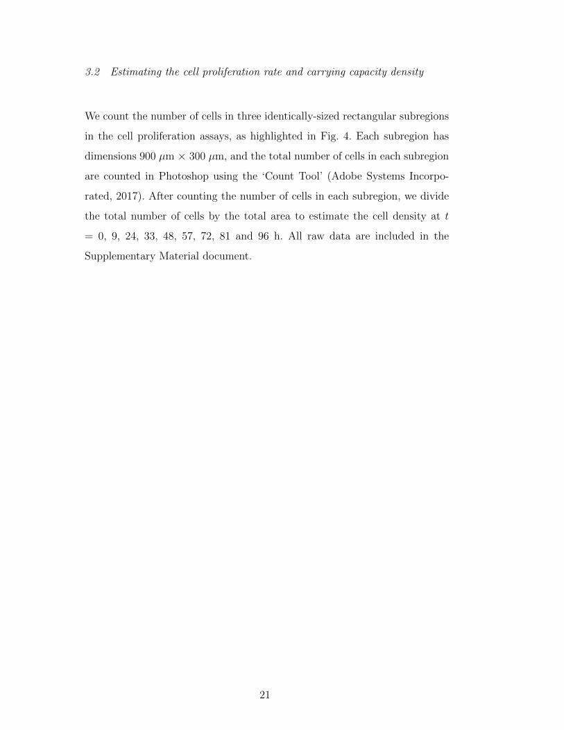
3.2 Estimating the cell proliferation rate and carrying capacity density

We count the number of cells in three identically-sized rectangular subregions

in the cell proliferation assays, as highlighted in Fig. 4. Each subregion has

dimensions 900 µm × 300 µm, and the total number of cells in each subregion

are counted in Photoshop using the ‘Count Tool’ (Adobe Systems Incorpo-

rated, 2017). After counting the number of cells in each subregion, we divide

the total number of cells by the total area to estimate the cell density at t

= 0, 9, 24, 33, 48, 57, 72, 81 and 96 h. All raw data are included in the

Supplementary Material document.

21

h 84 = th 42 = th 0 = t

h 69 = th 27 = t

)c()b()a(

)f()e()d(0010

Time (h)0

0.5

1

1.5

Cel

l den

sity

(cel

ls/μ

m2 )

×10-3

Yellow boxRed boxBlue boxAverage

20 40 60 80

Fig. 4. Estimating r and K. (a) - (e) Series of images showing the progression of the proliferation assays. The time at which the image

is recorded is indicated, and the scale bar corresponds to 500 µm. In each subfigure, three 900 µm × 300 µm subregions, highlighted

with yellow, red and blue rectangles, respectively, are superimposed on the experimental image. Manual cell counting is used to estimate

the number of cells in each subregion. (f) Cell density information is obtained at t = 0, 9, 24, 33, 48, 57, 72, 81 and 96 h.

22

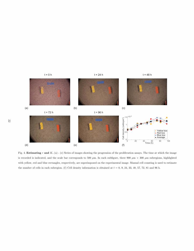
Using the data from the cell proliferation assay, we calibrate the solution of the

logistic growth model to the cell density information in all three subregions, as

shown in Fig. 4(f). This procedure allows us to estimate the cell proliferation

rate r, and the carrying capacity density K. To calibrate the model we form a

least–squares measure of the discrepancy between the solution of the logistic

growth model and the cell density data in each of the three subregions. This

least–squares measure is given by

E(r,K) =8∑

l=1

[Cmodel(tl)− Cdata(tl)

]2, (8)

where l is an index that indicates the number of time points. To find values

of r and K that minimise E(r,K), we use the MATLAB function lsqcurvefit

(MathWorks, 2017) that is based on the Levenberg–Marquardt algorithm.

We always take care to ensure that the iterative method is insensitive to

our initial choice of r and K. We denote the minimum least–squares error

as Emin = E(r, K). To calibrate the logistic growth model to data from the

proliferation assay, we use data t = 0 in Fig. 4(f) as the initial condition in

Eq. (7), and match Eq. (7) to the rest of the data. We repeat this procedure

three times using experimental data from each of the three subregions. To

demonstrate the quality of the match between the experimental data and

the calibrated logistic growth model, we superimpose the experimental data

and Eq. (7) with the estimates of r and K for each subregion in Fig. 5. The

results indicate that the quality of match between the solution of the logistic

model and the experimental data is very good. Estimates of r and K for each

subregion are summarised in Table 2. Since the variation in r and K between

the three subregions is relatively small, we further average these estimates to

give overall estimates of r = 0.036 /h and K = 1.4× 10−3 cells/µm2. We note

that these estimates of r and K are consistent with previous estimates for 3T3

fibroblast cells (ATCC, 2017; Treloar et al., 2014).

23

0 100Time (h)

0

0.5

1

1.5

Cel

l den

sity

(cel

ls/μ

m2 ) ×10-3

20 40 60 80 0 100Time (h)

0.5

1

1.5

Cel

l den

sity

(cel

ls/μ

m2 ) ×10-3

20 40 60 80 0 100Time (h)

0.5

1

1.5

Cel

l den

sity

(cel

ls/μ

m2 ) ×10-3

20 40 60 80

r = 0.031K = 1.46 × 10ˉ3

(a) (b) (c)

r = 0.030K = 1.42 × 10ˉ3

r = 0.046K = 1.30 × 10ˉ3

ˉ

ˉˉ ˉ

ˉ ˉ

Fig. 5. Comparing the mathematical model prediction and experimental data for the proliferation assay. The solution of

the logistic growth model is calibrated to the data of cell density information in (a) yellow, (b) red, and (c) blue boxes shown in Fig

4. In each subfigure, the solid line represents the calibrated solution, and the individual markers represent the experimental data. The

least–squares estimates of r and K are shown in the text box.

24

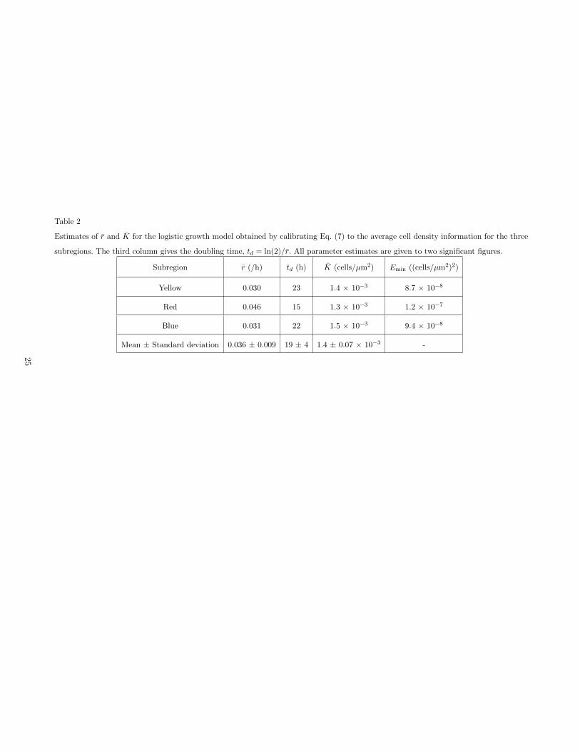
Table 2

Estimates of r and K for the logistic growth model obtained by calibrating Eq. (7) to the average cell density information for the three

subregions. The third column gives the doubling time, td = ln(2)/r. All parameter estimates are given to two significant figures.

Subregion r (/h) td (h) K (cells/µm2) Emin ((cells/µm2)2)

Yellow 0.030 23 1.4 × 10−3 8.7 × 10−8

Red 0.046 15 1.3 × 10−3 1.2 × 10−7

Blue 0.031 22 1.5 × 10−3 9.4 × 10−8

Mean ± Standard deviation 0.036 ± 0.009 19 ± 4 1.4 ± 0.07 × 10−3 -

25

3.3 Estimating the cell diffusivity

We now apply the discrete random walk model to mimic the sticker assays to

estimate the cell diffusivity. Our estimate of r in Section 3.2 allows us to specify

the ratio Pp/τ . We note that the individual values of Pp and τ are not uniquely

specified, but if we take τ = 0.05 h and Pp = 0.0018, then the proliferation rate

in the discrete model gives r = Pp/τ = 0.036 /h, as previously obtained. To

estimate D, we vary the parameters in the model to examine the behaviour of

the model when we consider the diffusivity parameter to lie within the interval,

500 ≤ D ≤ 2000 µm2/h. We choose this interval since the cell diffusivity for

fibroblast cells is thought to lie within this range (Johnston et al. 2016). Since

we have ∆ = 25 µm (Treloar et al., 2014), this interval of D corresponds

to an interval of 0.16 ≤ Pm ≤ 0.64, and we seek to find a value of Pm, and

hence D, which provides the best match between the discrete model and the

experimental images for each wound shape.

To simulate the sticker assays shown in Fig. 1, we use a lattice of size 10 mm

× 10 mm, which can be accommodated by setting I = 401 and J = 463

with ∆ = 25 µm. This simulation lattice is much smaller than the total size

of the domain, which is a circular tissue culture plate of diameter 35 mm.

However, the simulation lattice is considerably larger than the experimental

field of view, which is 5.56 mm × 3.71 mm, as shown in Fig. 1. Since the field

of view is smaller than the simulation domain, and cells in the experiment are

distributed uniformly away from the initial placement of the sticker, there will

be zero net flux of cells across the boundary of the field of view for all time

(Johnston et al., 2015). Therefore, specifying zero net flux conditions on the

boundary of the simulation lattice will mimic these experimental conditions.

To initialise the random walk simulations we note that the initial cell density in

the proliferation assays is approximately 40% of the carrying capacity density.

Therefore, we initialise the random walk simulations of the sticker assays by

26

randomly occupying each lattice site with probability 40%. To simulate how

the presence of the sticker prevents cells from occupying certain regions in

the experiment, we then we remove all agents within an appropriately sized

square, circle or equilateral triangle in the centre of the simulation lattice.

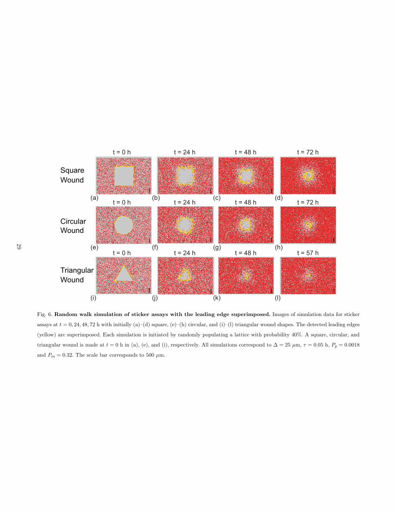
Figure 6 shows representative snapshots from the discrete model initialised

with the three different initial wound shapes. Although the simulation lattice

is larger than the experimental field of view, we present our results from the

discrete model by showing a region of the lattice that has the same dimen-

sions of the experimental field of view, as shown in Fig. 2. The snapshots of the

simulated wound closing for each initial wound shape show similar qualitative

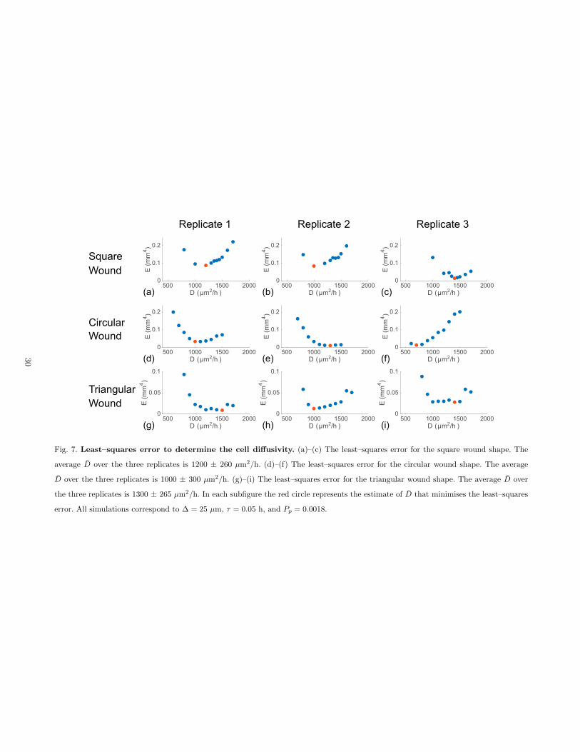
trends to those in the experimental images. To estimate D, we systematically

vary Pm in the simulations. For each value of Pm we generate a series of snap-

shots from the discrete model and use the ImageJ edge detection method to

find the location of the wound edge in each simulation snapshot. We estimate

D by examining a measure of the difference between the area enclosed by the

leading edge in the experimental images and averaged data from three iden-

tically prepared stochastic simulations. The measurement of discrepancy we

consider is given by

E(D) =1

L

L∑

l=1

[Amodel(tl)− Adata(tl)

]2, (9)

where Amodel(tl) is the average area of the wound estimated from the discrete

mathematical model at time tl, and Adata(tl) is the area of the wound estimated

from the experimental image at time tl. Here, l = 1, 2, . . . , L is an index

indicating the number of time points used to compare the experimental images

with images generated from the random walk model. Results in Fig. 7 show

E(D) for the three wound shapes, and we identify D as the value of D that

minimises the discrepancy, Emin = E(D). Our estimates of D are summarised

in Table 3. There are two notable features of these estimates: (1) The difference

between the average D for the three wound shapes is relatively small; and (2)

27

the range of estimated D for the three wound shapes overlap. Therefore, the

simplest explanation of our model calibration procedure is that our estimates

of D are effectively independent of the initial wound shape.

28

t = 0 h t = 24 h t = 48 h t = 72 h

t = 0 h t = 24 h t = 48 h t = 72 h

t = 0 h t = 24 h t = 48 h t = 57 h

(a) (b) (c) (d)

(e) (f) (g) (h)

(i) (j) (k) (l)

Square

Circular

Triangular

Wound

Wound

Wound

Fig. 6. Random walk simulation of sticker assays with the leading edge superimposed. Images of simulation data for sticker

assays at t = 0, 24, 48, 72 h with initially (a)–(d) square, (e)–(h) circular, and (i)–(l) triangular wound shapes. The detected leading edges

(yellow) are superimposed. Each simulation is initiated by randomly populating a lattice with probability 40%. A square, circular, and

triangular wound is made at t = 0 h in (a), (e), and (i), respectively. All simulations correspond to ∆ = 25 µm, τ = 0.05 h, Pp = 0.0018

and Pm = 0.32. The scale bar corresponds to 500 µm.

29

500 1000 1500 2000D (µm2/h )

0

0.1

0.2

E (m

m4 )

500 1000 1500 2000D (µm2/h )

0

0.1

0.2

E (m

m4 )

500 1000 1500 2000D (µm2/h )

0

0.1

0.2

E (m

m4 )

500 1000 1500 2000D (µm2/h )

0

0.1

0.2

E (m

m4 )

500 1000 1500 2000D (µm2/h )

0

0.1

0.2

E (m

m4 )

500 1000 1500 2000D (µm2/h )

0

0.1

0.2

E (m

m4 )

500 1000 1500 2000D (µm2/h )

0

0.05

0.1

E (m

m4 )

500 1000 1500 2000D (µm2/h )

0

0.05

0.1

E (m

m4 )

500 1000 1500 2000D (µm2/h )

0

0.05

0.1

E (m

m4 )

(a) (b) (c)

(d) (e) (f)

(g) (h) (i)

Replicate 1 Replicate 2 Replicate 3

Square

Circular

Triangular

Wound

Wound

Wound

Fig. 7. Least–squares error to determine the cell diffusivity. (a)–(c) The least–squares error for the square wound shape. The

average D over the three replicates is 1200 ± 260 µm2/h. (d)–(f) The least–squares error for the circular wound shape. The average

D over the three replicates is 1000 ± 300 µm2/h. (g)–(i) The least–squares error for the triangular wound shape. The average D over

the three replicates is 1300 ± 265 µm2/h. In each subfigure the red circle represents the estimate of D that minimises the least–squares

error. All simulations correspond to ∆ = 25 µm, τ = 0.05 h, and Pp = 0.0018.

30

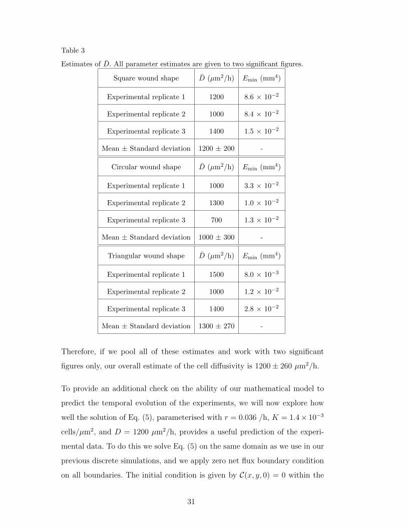
Table 3

Estimates of D. All parameter estimates are given to two significant figures.

Square wound shape D (µm2/h) Emin (mm4)

Experimental replicate 1 1200 8.6 × 10−2



Mean ± Standard deviation 1200 ± 200 -

Circular wound shape D (µm2/h) Emin (mm4)





Triangular wound shape D (µm2/h) Emin (mm4)





Therefore, if we pool all of these estimates and work with two significant

figures only, our overall estimate of the cell diffusivity is 1200± 260 µm2/h.

To provide an additional check on the ability of our mathematical model to

predict the temporal evolution of the experiments, we will now explore how

well the solution of Eq. (5), parameterised with r = 0.036 /h, K = 1.4× 10−3

cells/µm2, and D = 1200 µm2/h, provides a useful prediction of the experi-

mental data. To do this we solve Eq. (5) on the same domain as we use in our

previous discrete simulations, and we apply zero net flux boundary condition

on all boundaries. The initial condition is given by C(x, y, 0) = 0 within the

31

initial wound area, and C(x, y, 0) = 0.4K outside the wound area. Using the

method of lines, Eq. (5) is discretised with a central difference approximation

with uniform node spacing, δ. Details of the discretisation are provided in the

Supplementary Material document. The resulting system of coupled nonlinear

ordinary differential equations is solved using MATLAB function ode45 with

tolerance ε (MathWorks, 2017). We superimpose the numerical solution of Eq.

(5) on the experimental images by showing the contour, C(x, y, t) = 0.2K, at

various times. This contour corresponds to a density of 20% of the confluent

density, and we find that this choice of contour provides a good estimate of

the density at the leading edge as detected by the ImageJ edge detection al-

gorithm. Details of the procedure used to provide this estimate are given in

the Supplementary Material document. Overall, comparing the solution of Eq.

(5) presented in terms of the contour of the leading edge density and the ex-

perimental images suggests that our mathematical model, parameterised with

a unique combination of parameters, can predict the time evolution of the

wound area for all three initial wound shapes.

32

t = 0 h t = 24 h t = 48 h t = 72 h

t = 0 h t = 24 h t = 48 h t = 72 h

t = 0 h t = 24 h t = 48 h t = 57 h

(a) (b) (c) (d)

(e) (f) (g) (h)

(i) (j) (k) (l)

Fig. 8. Contour plot of numerical solutions of Eq. (2) for the sticker assays. The wound closure with initially square, cir-

cular and triangular wound shapes are shown in (a)–(d), (e)–(h), and (i)–(l), respectively. The blue contour plot that corresponds to

C(x, y, t) = 0.2K is superimposed onto the detected edge in each subfigure. The scale bar corresponds to 500 µm. The numerical solutions

of Eq. (5) is obtained with D = 1200 µm2/h, r = 0.036 /h, K = 1.4× 10−3 cells/µm2, δ = 10 µm, and ε = 1× 10−5.

33

4 Conclusions

Wound healing assays are routinely used to study the collective cell migration

during wound closing (Keese et al., 2004; Singh et al., 2003). While real wounds

take on arbitrary shapes, wound healing assays are usually limited to just one

particular wound shape (Gough et al., 2011; Jin et al., 2016; Johnston et

al., 2015, 2016; Keese et al., 2004; Kramer et al., 2013; Riahi et al., 2012;

Sengers et al., 2007). When we interpret results from a wound healing assay,

an implicit assumption is always made. This assumption is that the results

from a particular assay, with a specific initial wound shape, would apply to

other wounds with a different initial shape. This implicit assumption is always

made, rarely stated and never examined in any detail. To explore the validity

of such an assumption, here we develop and perform a new kind of wound

healing assay, called a sticker assay, to examine wound healing with various

initial wound shapes.

Previous experimental studies present the results from wound healing assays

by reporting the time evolution of wound area as the wound closes (Leu et al.,

2012; Ueck et al., 2017; Yarrow et al., 2004). When we report the results from

our sticker assays in this standard way, we find that the area of the circular,

square and triangular wounds close linearly with time. However, the rate of

wound closure is very different between the three initial wound shapes. With-

out further examination, this kind of standard data might suggest that the

mechanisms driving wound closure could depend on the initial wound shape.

To provide further information about this question we attempt to quantify the

relevant mechanisms in the experiments by calibrating the solution of a dis-

crete random walk model, and the continuum-limit description of this model,

to the experimental data.

In summary, we find that our estimates of the cell diffusivity for each initial

wound area are similar, and the range of cell diffusivity obtained from the

34

three experimental replicates for each initial wound shape overlap. Therefore,

the simplest possible explanation of our results is that the two-dimensional

Fisher-Kolmogorov model with one unique choice of parameters provides a

good match of the experimental data. Therefore, while the temporal wound

area data depends on the initial wound shape, the underlying mechanisms

that drive the behaviour of the cell populations (i.e. cell proliferation and cell

migration) do not depend on the initial wound shape.

To provide a confirmation of our results, we solve the two–dimensional Fisher-

Kolmogorov equation with our single set of parameter values for each initial

wound shape. To check that the model matches the experimental data we su-

perimpose a particular contour from the numerical solution with C(x, y, t) =

0.20K onto the experimental images. This comparison implies that the continuum-

limit PDE description of our random walk model, parameterised with a unique

combination of parameters, provides a good match to the experimental data.

Again, this result implies that while the temporal wound area data depends

on the initial wound shape, the fundamental transport mechanism that drive

the wound healing processes not to depend on the initial wound shape.

Our approach to modelling experimental data is always to use the simplest

possible mathematical model that describes the key features in the experi-

ment. In this case we use a discrete exclusion process in which agents un-

dergo unbiased migration and unbiased proliferation. The unbiased exclusion

process-based motility mechanism gives rise to a linear diffusion term in the

continuum limit PDE, and the exclusion process-based proliferation mecha-

nism gives rise to a logistic source term. Therefore, the continuum limit PDE

is the two-dimensional Fisher-Kolmorogov model, and our data suggests that

this model provides a good match to the experimental observations. However,

we are well aware that other studies suggest that the Porous–Fisher model,

which has a nonlinear diffusion term, might be preferable since this model

gives rise to well-defined sharp fronts (Maini et al., 2004a, 2004b; Sengers

35

et al., 2007). Since we find that the simpler model with a linear diffusion

continuum-limit provides a good match to the experimental data, we do not

pursue using any kind of more complicated mathematical model at this stage.

From a mathematical perspective, the geometry of our wound healing assay

is reminiscent of a hole-closing problem. These problems are characterised

by partial differential equations being applied outside of a two-dimensional

“hole” which shrinks inwards in time. Typically, these are formulated as mov-

ing boundary problems with Stefan-type boundary conditions (Dallaston and

McCue, 2013; McCue and King, 2011) or, alternatively, nonlinear diffusion

problems with degenerate diffusive terms and sharp interfaces (Angenent et

al., 2001; Betelu et al., 2000; Witelski, 1995). As an alternative to using a dis-

crete random walk model, it would be interesting to model our experimental

data as a hole-closing problem and explore the effects of cell migration and

proliferation on the geometry of the wound, as predicted by that model, as

the wound closes.

References

[1] Adobe Systems Incorporated. Count

objects in an image. http://helpx.adobe.com/photoshop/using/counting-objects-

image.html (Accessed: November 2017)

[2] Angenent, S.B., Aronson, D.G., Betelu, S.I., Lowengrub, J.S., 2001. Focusing of

an elongated hole in porous medium flow. Physica D. 151, 228–252.

[3] Ariano, P., Dalmazzo, S., Owsianik, G., Nilius, B., Lovisolo, D., 2011. TRPC

channels are involved in calcium-dependent migration and proliferation in

immortalized GnRH neurons. Cell Calcium. 49, 387–394.

[4] Ascione, F., Caserta, S., Guido, S., 2017. The wound healing assay revisited: A

transport phenomena approach. Chem Eng Sci. 160, 200–209.

36

[5] ATCC. NIH/3T3 (ATCC R©CRL–1658TM).

https://www.atcc.org/products/all/CRL-1658.aspx#generalinformation

(Accessed: November 2017).

[6] Bachstetter, A.D., Zhou, Z., Rowe, R.K., Xing, B., Goulding, D.S., Conley,

A.N., Sompol, P., Meier, S., Abisambra, J.F., Lifshitz, J., Watterson, D.M., 2016.

MW151 inhibited IL–1β levels after traumatic brain injury with no effect on

microglia physiological responses. PLOS ONE. 11, e0149451.

[7] Betelu, S.I., Aronson, D.G., Angenent, S.B., 2000. Renormalization study of two–

dimensional convergent solutions of the porous medium equation. Physica D. 138,

344–359.

[8] Cai, A.Q., Landman, K.A., Hughes, B.D., 2007. Multi-scale modelling of a wound

healing assay. J Theor Biol. 245, 576–594.

[9] Codling, E., Plank, M.J., and Benhamou, S., 2008. Random walk models in

biology. J Roy Soc Interface. 5, 813–835.

[10] Dallaston, M.C., McCue, S.W., 2013. Bubble extinction in Hele–Shaw flow with

surface tension and kinetic undercooling regularization. Nonlinearity. 26, 1639–

1665.

[11] Ferreira, T., Rasband, W., 2012.

ImageJ user guide. https://imagej.nih.gov/ij/docs/guide/index.html (Accessed:

November 2017).

[12] Fisher RA (1937). The wave of advance of advantageous genes. Ann Eugen. 7:

353–369.

[13] Gough, W., Hulkower, K., Lynch, R., Mcglynn, P., Uhlik, M., Yan, L., Lee,

J., 2011. A quantitative, facile, and high–throughput image–based cell migration

methods is a robust alternative to the scratch assay. J Biomol Screen. 16, 155–163.

[14] Jin, W., Shah, E.T., Penington, C.J., McCue, S.W., Chopin, L.K., Simpson,

M.J., 2016. Reproducibility of scratch assays is affected by the initial degree of

confluence: Experiments, modelling and model selection. J Theor Biol. 390, 136–

145.

37

[15] Jin, W., Shah, E.T., Penington, C.J., McCue, S.W., Maini, P.K., Simpson, M.J.,

2017. Logistic proliferation of cells in scratch assays is delayed. Bull Math Biol.

79, 1028–1050.

[16] Johnston, S.T., Shah, E.T., Chopin, L.K., McElwain, D.S., Simpson, M.J., 2015.

Estimating cell diffusivity and cell proliferation rate by interpreting IncuCyte

ZOOMTM assay data using the Fisher–Kolmogorov model. BMC Syst Biol. 9, 38.

[17] Johnston, S.T., Ross, J.V., Binder, B.J., McElwain, D.S., Haridas, P., Simpson,

M.J., 2016. Quantifying the effect of experimental design choices for in vitro

scratch assays. J Theor Biol. 400, 19–31.

[18] Jones, L.J., Gray, M., Yue, S.T., Haugland, R.P., Singer, V.L., 2001. Sensitive

determination of cell number using the CyQUANT R© cell proliferation assay. J

Immunol Methods. 254, 85–98.

[19] Jonkman, J.E., Cathcart, J.A., Xu, F., Bartolini, M.E., Amon, J.E., Stevens,

K.M., Colarusso, P., 2014. An introduction to the wound healing assay using

live–cell microscopy. Cell Adhes Migr. 8, 440–451.

[20] Katakowski, M., Zheng, X., Jiang, F., Rogers, T., Szalad, A., Chopp, M., 2010.

MiR–146b–5p suppresses EGFR expression and reduces in vitro migration and

invasion of glioma. Cancer Invest. 28,1024–1030.

[21] Keese, C.R., Wegener, J., Walker, S.R., Giaever, I., 2004. Electrical wound–

healing assay for cells in vitro. P Natl Acad Sci USA. 101, 1554–1559.

[22] Kolmogorov A, Petrovsky I, Piscounov N (1937). Etude de l’equation de la

diffusion avec croissance de la quantite de matiere et son application a un probleme

biologique. Moscow University Bulletin of Mathematics. 1: 1–25.

[23] Kramer, N., Walzl, A., Unger, C., Rosner, M., Krupitza, G., Hengstschlger, M.,

Dolznig, H., 2013. In vitro cell migration and invasion assays. Mutat Res Rev

Mutat Res. 752, 10–24.

[24] Lee, J., Wang, Y.L., Ren, F., Lele, T.P., 2010. Stamp wound assay for studying

coupled cell migration and cell debris clearance. Langmuir. 26, 16672–16676.

38

[25] Leu, J.G., Chen, S.A., Chen, H.M., Wu, W.M., Hung, C.F., Yao, Y.D., Tu,

C.S., Liang, Y.J., 2012. The effects of gold nanoparticles in wound healing with

antioxidant epigallocatechin gallate and α–lipoic acid. Nanomed–Nanotechnol. 8,

767–775.

[26] Liang, C.C., Park, A.Y., Guan, J.L., 2007. In vitro scratch assay: a convenient

and inexpensive method for analysis of cell migration in vitro. Nat Protoc. 2,

329–333.

[27] Madison, J.B., Gronwall, R.R., 1992. Influence of wound shape on wound

contraction in horses. Am J Vet Res. 53, 1575–1578.

[28] Maini, P.K., McElwain, D.L.S., Leavesley, D.I., 2004a. Traveling wave model to

interpret a wound–healing cell migration assay for human peritoneal mesothelial

cells. Tissue Eng. 10, 475–482.

[29] Maini, P.K., McElwain, D.L.S., Leavesley, D.I., 2004b. Travelling waves in a

wound healing assay. Appl Math Lett. 17, 575–580.

[30] Mamouni, J., Yang, L., 2011. Interdigitated microelectrode–based microchip for

electrical impedance spectroscopic study of oral cancer cells. Biomed Microdevices.

13, 1075–1088.

[31] MathWorks. Ode45. https://au.mathworks.com/help/matlab/ref/ode45.html


[32] MathWorks. Lsqcurvefit.

https://au.mathworks.com/help/optim/ug/lsqcurvefit.html (Accessed: November

2017).

[33] McCue, S.W., King, J.R., 2011. Contracting bubbles in Hele–Shaw cells with a

power–law fluid. Nonlinearity. 24, 613–641.

[34] O’Dea, R., Jing, J.R., 2012. Continuum limits of pattern formation in

hexagonal-cell monolayers. J Math Biol. 64, 579–610.

[35] Painter, K.J., Sherratt, J.A. 2003. Modelling the movement of interacting cell

populations. J Theor Biol. 225, 327–339.

39

[36] Painter, K.J., Hillen, T. 2002. Volume-filling and quorum-sensing in models for

chemosensitive movement. Canadian Applied Mathematics Quarterly. 10, 501–

543.

[37] Riahi, R., Yang, Y., Zhang, D.D., Wong, P.K., 2012. Advances in wound–healing

assays for probing collective cell migration. J Lab Autom. 17, 59–65.

[38] Sengers, B.G., Please, C.P., Oreffo, R.O.C., 2007. Experimental characterization

and computational modelling of two-dimensional cell spreading for skeletal

regeneration. J R Soc Interface. 4, 1107–1117.

[39] Sheardown, H., Cheng, Y.-L., 1996. Mechanisms of corneal epithelial wound

healing. Chem Eng Sci. 51, 4517-4529.

[40] Sherratt JA, Murray JD (1990). Models of epidermal wound healing. Proc R

Soc B. 241: 29–36.

[41] Singh, S.K., Clarke, I.D., Terasaki, M., Bonn, V.E., Hawkins, C., Squire, J.,

Dirks, P.B., 2003. Identification of a cancer stem cell in human brain tumors.

Cancer Res. 63, 5821–5828.

[42] Simpson, M.J., Landman, K.A., Hughes, B.D., 2010. Cell invasion with

proliferation mechanisms motivated by time–lapse data. Physica A. 389, 3779–

3790.

[43] Swanson, K.R., Bridge, C., Murray, J.D., Alvord, Jr. E.,C. 2003. Virtual and

real brain tumors: using mathematical modeling to quantify glioma growth and

invasion. J Neurol Sci. 216, 1–10.

[44] Swanson K.R., 2008. Quantifying glioma cell growth and invasion in vitro. Math

Comput Model. 47, 638–648.

[45] Treloar, K.K., Simpson, M.J., 2013. Sensitivity of edge detection methods for

quantifying cell migration assays. PLOS ONE. 8, e67389.

[46] Treloar, K.K., Simpson, M.J., McElwain, D.L.S., Baker, R.E., 2014. Are in vitro

estimates of cell diffusivity and cell proliferation rate sensitive to assay geometry?

J Theor Biol. 356, 71–84.

40

[47] Tremel, A., Cai, A., Tirtaatmadja, N., Hughes, B.D., Stevens, G.W., Landman,

K.A., OConnor, A.J., 2009. Cell migration and proliferation during monolayer

formation and wound healing. Chem Eng Sci. 64, 247–253.

[48] Ueck, C., Volksdorf, T., Houdek, P., Vidal-y-Sy, S., Sehner, S., Ellinger,

B., Lobmann, R., Larena-Avellaneda, A., Reinshagen, K., Ridderbusch, I.,

Kohrmeyer, K., 2017. Comparison of in–vitro and ex–vivo wound healing assays

for the investigation of diabetic wound healing and demonstration of a beneficial

effect of a triterpene extract. PLOS ONE. 12, e0169028.

[49] van der Meer, A.D., Vermeul, K., Poot, A.A., Feijen, J., Vermes, I., 2010. A

microfluidic wound–healing assay for quantifying endothelial cell migration. Am

J Physiol–Heart C. 298, H719–725.

[50] Vedula, S.R., Ravasio, A., Lim, C.T., Ladoux, B., 2013. Collective cell

migration: a mechanistic perspective. Physiology. 28, 370-379.

[51] Walter, M.N., Wright, K.T., Fuller, H.R., MacNeil, S., Johnson, W.E., 2010.

Mesenchymal stem cell–conditioned medium accelerates skin wound healing: an

in vitro study of fibroblast and keratinocyte scratch assays. Exp Cell Res. 316,

1271–1281.

[52] Witelski, T.P., 1995. Merging traveling waves for the porous–Fisher’s equation.

Appl Math Lett. 8, 57–62.

[53] Yarrow, J.C., Perlman, Z.E., Westwood, N.J., Mitchison, T.J., 2004. A high–

throughput cell migration assay using scratch wound healing, a comparison of

image–based readout methods. BMC Biotechnol. 4, 21.

41

Supplementary Material

Wang Jin1, Kai-Yin Lo2, Shih–En Chou2, Scott W McCue1

∗Matthew J Simpson1

1 School of Mathematical Sciences, Queensland University of Technology (QUT)

Brisbane, Queensland 4000, Australia.

2 Department of Agricultural Chemistry, National Taiwan University

Taipei 10617, Taiwan.

∗ Corresponding authorEmail address: [email protected], Telephone + 617 31385241,

Fax + 617 3138 2310 (∗Matthew J Simpson1).

Preprint submitted to Elsevier 12 March 2018

arX

iv:1

711.

0716

2v1

[q-

bio.

CB

] 2

0 N

ov 2

017

1 Experimental data: Wound area

We show the experimental images with the detected wound edge at t =

0, 24, 48, 72 h in Figs. 1–3. The estimated wound areas at all the recorded

experimental time points, i.e. t = 0, 9, 24, 33, 48, 57, 72 h, are listed in Tables

1–3 for the square, circular, and triangular wound shapes, respectively.

2

t = 0 h t = 24 h t = 48 h t = 72 h

(a) (b) (c) (d)

(e) (f) (g) (h)

(i) (j) (k) (l)

Replicate 1

Replicate 2

Replicate 3

Fig. 1. Experimental images of square wound shape with detected wound area. (a)–(d) Replicate 1. (e)–(h) Replicate 2.

(i)–(l) Replicate 3. The solid yellow line represents the detected wound edge using ImageJ (Ferreira and Rasband, 2012). The scale bar

corresponds to 500 µm

3

t = 0 h t = 24 h t = 48 h t = 72 h

t = 0 h t = 24 h t = 48 h t = 57 h

(a) (b) (c) (d)

(e) (f) (g) (h)

(i) (j) (k) (l)

t = 0 h t = 24 h t = 48 h t = 72 h

Replicate 1

Replicate 2

Replicate 3

Fig. 2. Experimental images of circular wound shape with detected wound area. (a)–(d) Replicate 1. (e)–(h) Replicate 2.



4

t = 0 h t = 24 h t = 48 h t = 57 h

(a) (b) (c) (d)

(e) (f) (g) (h)

(i) (j) (k) (l)

Replicate 1

Replicate 2

Replicate 3

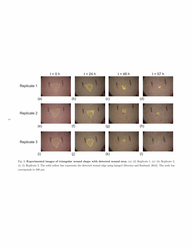
Fig. 3. Experimental images of triangular wound shape with detected wound area. (a)–(d) Replicate 1. (e)–(h) Replicate 2.



5

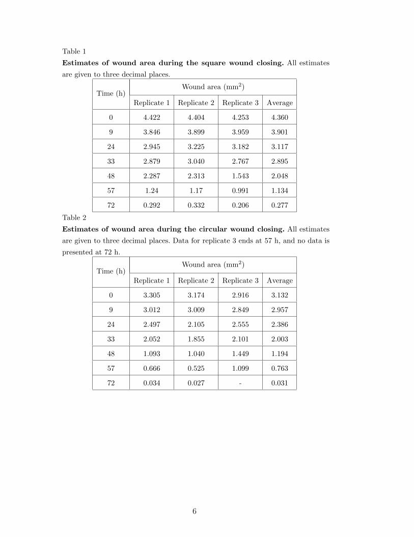
Table 1

Estimates of wound area during the square wound closing. All estimates

are given to three decimal places.

Time (h)Wound area (mm2)

Replicate 1 Replicate 2 Replicate 3 Average

0 4.422 4.404 4.253 4.360

9 3.846 3.899 3.959 3.901

24 2.945 3.225 3.182 3.117

33 2.879 3.040 2.767 2.895

48 2.287 2.313 1.543 2.048

57 1.24 1.17 0.991 1.134

72 0.292 0.332 0.206 0.277

Table 2

Estimates of wound area during the circular wound closing. All estimates

are given to three decimal places. Data for replicate 3 ends at 57 h, and no data is

presented at 72 h.



0 3.305 3.174 2.916 3.132

9 3.012 3.009 2.849 2.957

24 2.497 2.105 2.555 2.386

33 2.052 1.855 2.101 2.003

48 1.093 1.040 1.449 1.194

57 0.666 0.525 1.099 0.763

72 0.034 0.027 - 0.031

6

Table 3

Estimates of wound area during the triangular wound closing. All estimates

are given to three decimal places.



0 1.569 1.756 1.743 1.689

9 1.363 1.487 1.411 1.420

24 0.851 0.963 1.060 0.958

33 0.561 0.786 0.773 0.707

48 0.164 0.193 0.063 0.140

57 0.055 0.068 0.010 0.044

2 Experimental data: Cell density information

In Table 4 we show the cell density information in the three chosen subregions

in the proliferation assay, which is shown in Fig. 1 in the main manuscript.

Each subregion has dimensions 900 µm × 300 µm. Cells in each subregion are

counted in Photoshop using the ‘Count Tool’ (Adobe Systems Incorporated,

2017). After counting the number of cells in each subregion, we divide the

total number of cells by the total area to estimate the cell density at t = 0, 9,

24, 33, 48, 57, 72, 81 and 96 h.

7

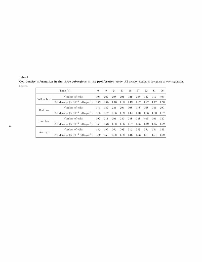
Table 4

Cell density information in the three subregions in the proliferation assay. All density estimates are given to two significant

figures.

Time (h) 0 9 24 33 48 57 72 81 96

Yellow boxNumber of cells 195 202 298 291 321 288 342 317 404

Cell density (× 10−3 cells/µm2) 0.72 0.75 1.10 1.08 1.19 1.07 1.27 1.17 1.50

Red boxNumber of cells 175 182 231 294 308 378 368 351 290


Blue boxNumber of cells 192 211 291 286 288 338 403 391 330


AverageNumber of cells 185 192 265 293 315 333 355 334 347


8

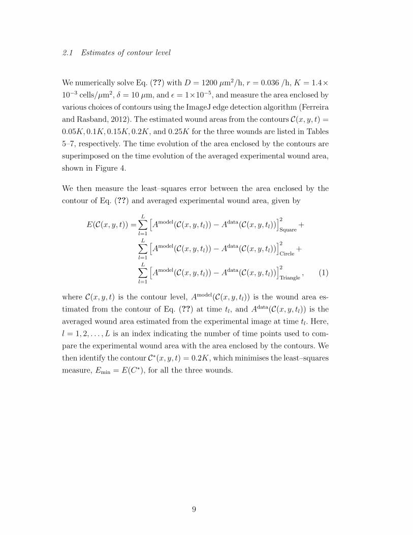
2.1 Estimates of contour level

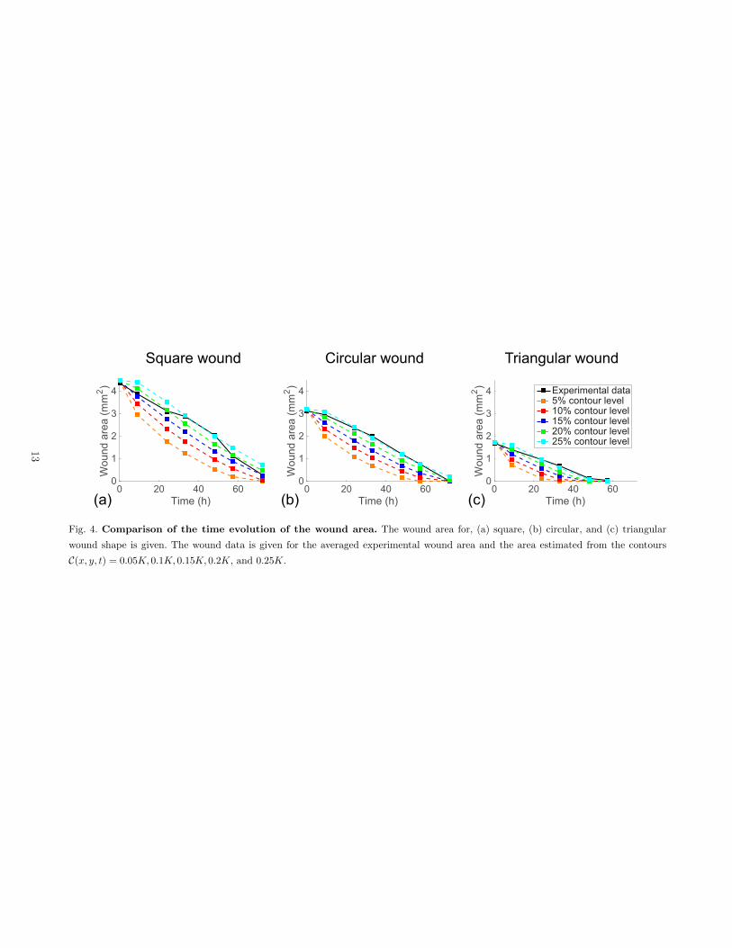
We numerically solve Eq. (??) with D = 1200 µm2/h, r = 0.036 /h, K = 1.4×10−3 cells/µm2, δ = 10 µm, and ε = 1×10−5, and measure the area enclosed by

various choices of contours using the ImageJ edge detection algorithm (Ferreira

and Rasband, 2012). The estimated wound areas from the contours C(x, y, t) =0.05K, 0.1K, 0.15K, 0.2K, and 0.25K for the three wounds are listed in Tables

5–7, respectively. The time evolution of the area enclosed by the contours are

superimposed on the time evolution of the averaged experimental wound area,

shown in Figure 4.

We then measure the least–squares error between the area enclosed by the

contour of Eq. (??) and averaged experimental wound area, given by

E(C(x, y, t)) =L∑

l=1

[Amodel(C(x, y, tl))− Adata(C(x, y, tl))

]2Square

+

L∑

l=1


]2Circle

+

L∑

l=1


]2Triangle

, (1)

where C(x, y, t) is the contour level, Amodel(C(x, y, tl)) is the wound area es-

timated from the contour of Eq. (??) at time tl, and Adata(C(x, y, tl)) is the

averaged wound area estimated from the experimental image at time tl. Here,

l = 1, 2, . . . , L is an index indicating the number of time points used to com-

pare the experimental wound area with the area enclosed by the contours. We

then identify the contour C∗(x, y, t) = 0.2K, which minimises the least–squares

measure, Emin = E(C∗), for all the three wounds.

9

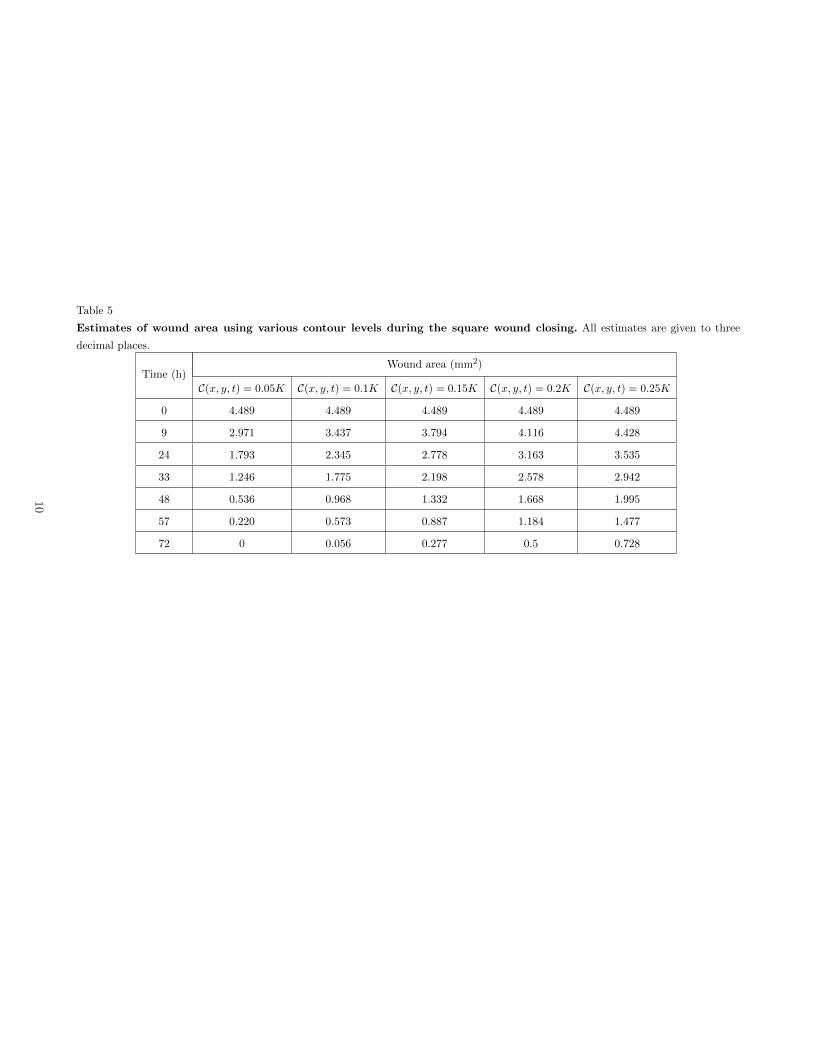
Table 5

Estimates of wound area using various contour levels during the square wound closing. All estimates are given to three

decimal places.


C(x, y, t) = 0.05K C(x, y, t) = 0.1K C(x, y, t) = 0.15K C(x, y, t) = 0.2K C(x, y, t) = 0.25K

0 4.489 4.489 4.489 4.489 4.489

9 2.971 3.437 3.794 4.116 4.428

24 1.793 2.345 2.778 3.163 3.535

33 1.246 1.775 2.198 2.578 2.942

48 0.536 0.968 1.332 1.668 1.995

57 0.220 0.573 0.887 1.184 1.477

72 0 0.056 0.277 0.5 0.728

10

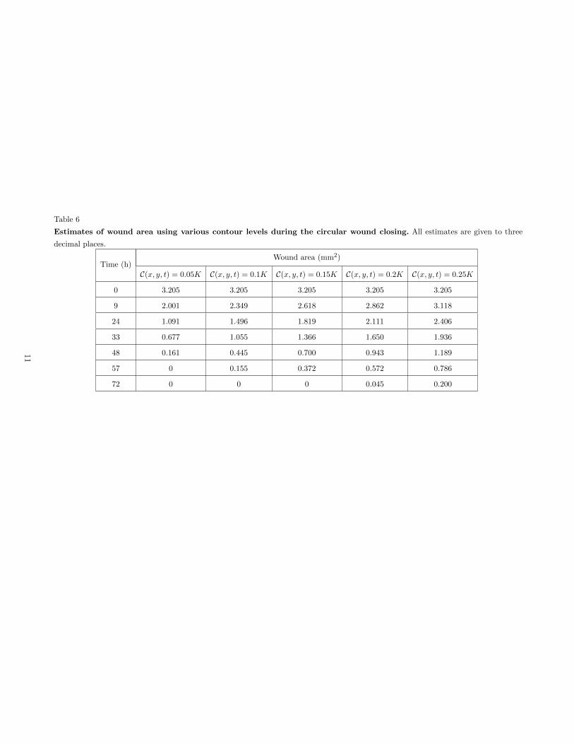
Table 6

Estimates of wound area using various contour levels during the circular wound closing. All estimates are given to three

decimal places.



0 3.205 3.205 3.205 3.205 3.205

9 2.001 2.349 2.618 2.862 3.118

24 1.091 1.496 1.819 2.111 2.406

33 0.677 1.055 1.366 1.650 1.936

48 0.161 0.445 0.700 0.943 1.189

57 0 0.155 0.372 0.572 0.786

72 0 0 0 0.045 0.200

11

Table 7

Estimates of wound area using various contour levels during the triangular wound closing. All estimates are given to three

decimal places.



0 1.757 1.757 1.757 1.757 1.757

9 0.713 0.981 1.203 1.408 1.616

24 0.129 0.354 0.566 0.775 0.989

33 0 0.088 0.255 0.431 0.617

48 0 0 0 0 0.082

57 0 0 0 0 0

12

0 20 40 60Time (h)

0

1

2

3

4

Wou

nd a

rea

(mm

2 )

0 20 40 60Time (h)

0

1

2

3

4

Wou

nd a

rea

(mm

2 )

0 20 40 60Time (h)

0

1

2

3

4

Wou

nd a

rea

(mm

2 ) Experimental data5% contour level10% contour level15% contour level20% contour level25% contour level

Square wound Circular wound Triangular wound

(a) (b) (c)

Fig. 4. Comparison of the time evolution of the wound area. The wound area for, (a) square, (b) circular, and (c) triangular

wound shape is given. The wound data is given for the averaged experimental wound area and the area estimated from the contours

C(x, y, t) = 0.05K, 0.1K, 0.15K, 0.2K, and 0.25K.

13

References

[1] Adobe Systems Incorporated. Count

objects in an image. http://helpx.adobe.com/photoshop/using/counting-objects-

image.html (Accessed: November 2017)

[2] Ferreira, T., Rasband, W., 2012.

ImageJ user guide. https://imagej.nih.gov/ij/docs/guide/index.html (Accessed:

November 2017).

[3] MathWorks. Ode45. https://au.mathworks.com/help/matlab/ref/ode45.html


14

the role of initial geometry in experimental models of ... · wound healing assays are initiated by...

Documents