1

The Role of Infrastructure Capital in China’s Regional Economic Growth

Yingying Shi

Michigan State University

shiyingy@msu.edu

Selected Paper prepared for presentation at the International Association of Agricultural Economists(IAAE) Triennial Conference, Foz do Iguaçu, Brazil, 18-24 August, 2012.

Copyright 2012 by Yingying Shi. All rights reserved. Readers may make verbatim copies of this documentfor non-commercial purposes by any means, provided that this copyright notice appears on all suchcopies.

2

Abstract

This paper investigates the role of infrastructure capital in China’s regional economic development during

1990 to 2009 in a neoclassical economic growth model. Four types of infrastructure capital are discussed;

electricity, road, rail, and land-line telephone. The results support a positive role of infrastructure in

improving economic wellbeing in China. It shows that infrastructure has contributed to the convergence

among China’s provinces. However, declining growth momentum from rapid increase of road infrastructure,

in particular for the Western region, suggests that road development in the region has been growing too fast.

The results counter the conventional wisdom of “road leads to prosperity” widely accepted among national

and local governments in China. Thus, the seemingly productive infrastructure capital, when invested beyond

a proper level or speed, will become unproductive. The results resonate with the theoretical literature on the

inverse U shaped growth impact of infrastructure capital and the dominant “crowding out” of private capital

if there is too much infrastructure. They also address the puzzle in the current literature debates as to the

direction and magnitude of the growth impact of infrastructure capital.

Keywords: infrastructure, economic growth, regional inequality, China

3

Contents

I. Introduction.............................................................................................................................................................. 6

II. Provincial infrastructure coverage and regional economic growth in China................................... 8

1. Regional growth performance............................................................................................................................. 8

2. The role of infrastructure and its historical development .............................................................................. 9

3. Infrastructure coverage ...................................................................................................................................... 11

III. The Model .......................................................................................................................................................... 14

IV. Empirical analysis ............................................................................................................................................ 16

i. Description of variables.................................................................................................................................. 16

ii. Regression analysis.......................................................................................................................................... 20

1. Average effect of infrastructure capital on China’s provincial growth .................................................. 20

2. Regional impact of infrastructure capital .................................................................................................... 24

3. The catching up process ................................................................................................................................28

4. Marginal effects of an increase in infrastructure network........................................................................ 28

iii Alternative specifications and results ............................................................................................................. 32

1. Endogenous investment decision ................................................................................................................ 32

2. Road classifications and cell-phone usage .................................................................................................. 33

V. Conclusions ............................................................................................................................................................ 34

APPENDIX ...................................................................................................................................................................... 35

REFERENCES:................................................................................................................................................................43

4

List of TablesTable 1 Selected infrastructure stock indicators across regions ............................................................................... 11Table 2 Average transport freight and passenger traffic across regions .................................................................. 12Table 3 Description of Variables.................................................................................................................................... 18Table 4 Time series properties of the variables............................................................................................................ 19Table 5 Average effect of infrastructure capital on real per capita economic growth........................................... 21Table 6 Regional impact of infrastructure capital........................................................................................................ 26Table 7 Marginal growth effect to an increase in the stock or growth rate of infrastructure capital .................. 29Table 8 Impact of infrastructure capital with endogenous investment.................................................................... 32Table 9 Average effect of infrastructure capital on real per capita economic growth........................................... 37Table 10 Road classifications and cell phone coverage .............................................................................................. 40

5

List of FiguresFigure 1 GDP per capita across China’s provinces 1990 vs. 2009 ............................................................................. 8Figure 2 Growth disparity among China’s provinces 1990-2009............................................................................... 9Figure 3 Map of China ..................................................................................................................................................... 35Figure 4 Types of infrastructure capital and GDP per capita.................................................................................... 36

6

I. Introduction

The literature often gives mixed results on the impact of infrastructure capital on economic development. Onthe one hand, the benefits of public infrastructure have long been recognized by classical studies on economicdevelopment. Rosenstein-Rodan (1943) and Nurkse (1952) and Hirschman (1957) have argued for a positiverole of infrastructure capital. Large amount of infrastructure investment is regarded as a necessity before allother types of investment are possible. The nature of infrastructure investment, which requires large sunkcosts and whose benefits usually cover a large number of people, is considered best with public provision.Samuelson (1954) in his classical studies on the pure theory of public expenditure has argued that theoreticallythere is no market solution to the optimal provision of collective consumption goods and they are better leftwith public hands.

On the other hand, Aschauer (1989a) finds that the infrastructure capital can have a dominant “crowding-out”effect on private investment. The usual complementary role of infrastructure capital is merely the result of adominant “crowding-in” effect, which can be reversed. Barro(1990) using an endogenous growth modelsuggests there are conflicting forces of infrastructure investment that result in an inverse U-shape of itsgrowth impact. An increase in public infrastructure initially raises growth rate, but then causes the growth rateto decline when infrastructure investment is beyond a certain level.

Such mixed results also manifest itself in the empirical literature. During the last wave of debate on the role ofinfrastructure in the early 1990s, Aschauer (1989b) provides results supporting the intuition that infrastructurehas a positive role to play in the economic development of the 50 U.S. states. His results were challenged byHoltz-Eakin (1994), who concludes with no significant relationship between public capital and privateproductivity for 48 states in the U.S. over 17 years. A number of studies that follow give a quite diverse anduncertain picture of the role of infrastructure as reviewed in Fisher (1997).

Other economists have looked beyond the boundary of developed countries and explore a variety ofexperiences from the developing world. The last major wave of infrastructure investment led by Asian andother developing countries in the early 1990s has provided rich resources to reveal the nature and role ofinfrastructure in much wider and diversified contexts. An obvious example comes from the sharp contrastbetween China and India. The former relies much on massive public spending as an “engine” of economicgrowth and an accommodating reaction to huge increasing domestic demand. The result is phenomenalchanges in its landscape from the start of its economic reform in the early 1980s. The latter, however, hasseen comparable economic growth over the last decade, but with a sluggish public sector where ever growingtraffic jams and mismanaged public infrastructure are commonplace, alongside with the prospering privatesectors.

Cross country study of the relationship between the composition of public expenditure and growth in 43developing countries over 20 years by Devarajan, Swaroop and Zou (1996) has shown that contrary to ourconventional thoughts increasing the share of current spending has large and significant impact on growthwhile increasing capital spending shares exerts negative influence on growth. While their study focuses on thecomposition but not the level of public spending, it shows that developing countries have a different andinteresting story to tell. Moreover, cross country studies on public infrastructure investment often ignore thediversity and dynamics that are within each country, despite giving new perspectives and understandings onthe role of infrastructure, such as Calderon and Serven (2004).

7

Empirical studies on the infrastructure growth nexus in China are quite limited. Among the few, Demurger(2001) reviews the development of China’s transport infrastructure and its relationship with regionaleconomic growth in 24 provinces, excluding municipalities, from 1985 to 1998. Zhang et al (2006)investigates the determinants of infrastructure investments at the sub-national level with a political economicframework, but they haven’t assessed the growth impact of infrastructure capital. Bai and Qian (2010) presentan in-depth description of the infrastructure development in electricity, highways and railways at the nationallevel with a review on the institutional features of these sectors, but no empirical testing has been performed.Fan (2004) explores the impact of infrastructure capital on economic development in rural China.

This paper, therefore, builds upon the existing studies on the infrastructure and growth nexus and explores indepth China’s provincial economic growth and the role of infrastructure capital. It discusses four types ofinfrastructure - electricity, road, rail and telecommunications - knowing that any simple look at only one ofthem would miss the fact that they often influence each other. It covers the time span from 1990 to 2009when the major reforms and economic progressions come into full play. Rather than taking the nation as awhole, it regards each of its 27 provinces and 4 municipalities as both independent and interconnectedentities. This is more of the case when the country decides, from its central planning practices, to leave moredecisions to the sub-national and local governments and to delineate enterprises from the government bodiesso that they can react to the market conditions with more flexibility and effectiveness.

The paper asks the following questions. Have these four types of infrastructure played a positive role for theconvergence of China’s provinces? How much do different types of infrastructure contribute to theimprovement of their economic prospects? Do the effects vary with time and across different economicregions?

The paper proceeds as follows. Part II gives an account of the provincial growth performances and majornational reforms during the period under study. It then provides an overview of the infrastructuredevelopment across its geographic region. Part III presents a simple neoclassical model with infrastructurecapital as a basis for the empirical analysis. Part IV lets the data tell the story about the role of infrastructureand interprets the findings from regressions. Alternative specification tests are performed with resultsreported. A conclusion is in Part V.

8

II. Provincial infrastructure coverage and regional economic growth in China

1. Regional growth performance

China’s growth record has been well documented. Its GDP grew from RMB 1866.78 billion ($ 390.3 billion)in 1990 to RMB34050.69 billion (about $4984.7 billion) in 2009. Real GDP has been growing at an averagerate of over 10% during the time. The standard of living as measured by GDP per capita has grown fromRMB1, 644($343.7) to RMB 25,575 (about $3744) in 2009.

The growth performance of China, however, varies greatly across provinces1. Figure 1 shows the provincialreal GDP per capita in 1990 and 2009. On the whole, the Eastern region has been leading the economicgrowth, while the Central and Western regions, which cover over half of the land, have been lagging behind2.There is a wide gap among provinces. If the municipalities are excluded, which are at the same administrativelevel with the provinces, the lagging regions in the Western part of China have about one third of the percapita GDP of top provinces such as Zhejiang and Guangdong.

Figure 1 also shows the position of provinces relative to each other. The traditional resource rich heavy-industry endowed Northeastern provinces have been declining, while Henan in the Central region and InnerMongolia in the Western region have been among the fastest growing provinces. The majority of the Westernregion provinces, however, are continuously ranked at the bottom.

The reference lines in both graphs refer to the median level of per capita GDP in the respective years. Itshows that the majority of Eastern provinces have been growing much higher beyond the median level. TheNortheastern provinces, consistent with the above findings, are showing declining ranks among the provinces.The lagging Central and Western regions, on the whole are catching up, but the speed is much less than theEastern counterparts. Compared with the median level of per capita GDP, only Inner Mongolia has shownsignificant improvement in its rank. Most others are still below the median level of per capita GDP.

Figure 1 GDP per capita across China’s provinces 1990 vs. 2009

1 A map of China’s provinces can be found in Figure 3 in the appendix.2 The regions Eastern, Central, Western and Northeastern are classified according to their geographic locations, thenature and, virtually from the graph, performance of their economy. They are frequently named as the Four MajorEconomic Regions in China. This classification is also adopted by China’s statistical yearbooks. There are 10 provincesin the Eastern region, 6 in the Central, 12 in the Western region and 3 in the Northeastern region.

0 2,000 4,000 6,000Per capita GDP, yuan

Northeastern

Western

Central

Eastern

JilinHeilongjiang

Liaoning

GuizhouSichuan

ChongqingGuangxi

GansuShannxiYunnan

TibetNingxia

Inner MongoliaQinghaiXinjiang

HenanJiangxiAnhui

HunanShanxiHubei

HebeiHainanFujian

ShandongJiangsu

ZhejiangGuangdong

TianjinBeijing

Shanghai

Provincial GDP per capita 1990

0 20,000 40,000 60,000 80,000Per capita GDP, yuan

Northeastern

Western

Central

Eastern

HeilongjiangJilin

Liaoning

GuizhouGansu

YunnanTibet

GuangxiSichuanQinghaiXinjiangNingxia

ShannxiChongqing

Inner Mongolia

AnhuiJiangxiHunanHenanShanxiHubei

HainanHebeiFujian

ShandongGuangdong

ZhejiangJiangsu

TianjinBeijing

Shanghai

Provincial GDP per capita 2009

9

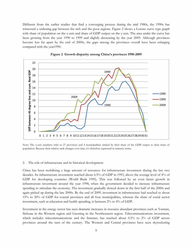
Different from the earlier studies that find a converging process during the mid 1980s, the 1990s haswitnessed a widening gap between the rich and the poor regions. Figure 2 shows a Lorenz curve type graphwith share of population on the x-axis and share of GDP output on the y-axis. The area under the curve hasbeen growing from the year 1990 to 1999 and slightly decreasing by the year 2009. Although provincesbecome less far apart by the end of 2000s, the gaps among the provinces overall have been enlargingcompared with the year1990.

Figure 2 Growth disparity among China’s provinces 1990-2009

Note: The x-axis numbers refer to 27 provinces and 4 municipalities ranked by their share of the GDP output to their share ofpopulation. Because their relative rank changes over time, it’s therefore expressed in numeric terms.

2. The role of infrastructure and its historical development

China has been mobilizing a large amount of resources for infrastructure investment during the last twodecades. Its infrastructure investment reached about 6.5% of GDP in 1993, above the average level of 4% ofGDP for developing countries (World Bank 1995). This was followed by an even faster growth ininfrastructure investment around the year 1998, when the government decided to increase infrastructurespending to stimulate the economy. The investment gradually slowed down in the first half of the 2000s andagain picked up during the late 2000s. By the end of 2009, investment in infrastructure had reached to about15% to 20% of GDP for coastal provinces and all four municipalities, whereas the share of social sectorinvestment, such as education and health spending, is between 2% to 4% of GDP.

Investment in the energy sector has seen dramatic increases in resource abundant provinces such as Yunnan,Sichuan in the Western region and Liaoning in the Northeastern region. Telecommunications investment,which includes telecommunications and the Internet, has reached about 0.5% to 2% of GDP acrossprovinces around the turn of the century. The Western and Central provinces have seen skyrocketing

1990

1999

2009

0

2

4

6

8

10

12

14

16

18

20

22

0 1 2 3 4 5 6 7 8 9 10111213141516171819202122232425262728293031

Diff

betw

een

45 d

egre

e lin

e an

d cu

m. R

eal G

DP

1990

1999

2009

10

transport investment. Their transport investment to GDP ratios have reached almost 5% while for the moredeveloped coastal provinces such as Jiangsu, the transport investment to GDP ratio is much less (for Jiangsu,the investment- GDP ratio is about 2%).

A number of factors have provided a favorable environment for infrastructure to grow in China. China hasgradually developed from an agrarian country with almost 50% population in agriculture into a manufacturingstate. The increasing labor force and foreign capitals in the industrial sectors requires cities to expand and tobe better equipped. Infrastructure bottlenecks have been felt in particular by the coastal cities such asShanghai and provinces such as Zhejiang. These areas respond by investing heavily in infrastructure, inparticular the transport infrastructure at a rate of over 40% per year recently. Such development, as shown inthe empirical analysis, does exert positive effect on the improvement of economic standards in those areas.

As an integral part of the Special Economic Zone (SEZ) development across China, infrastructuredevelopment has been undergoing three major stages. If the year from 1980 to 1989 marks the beginning ofthe historic establishment of four SEZs, the two decades from the year 1990 is twenty years of mushroomingSEZs spreading from the coastal to more inland and lagging provinces. At the beginning, barren land inremote villages designated as SEZs require large infrastructure investment to shape them into productioncenters. In the second stage, infrastructure is accommodating to the growth of an export oriented economy.Since many special zones are far away from the major economic centers, they need roads, railways and energyto support the export industries. The third stage comes when the economy grows to a more advanced level.Congestion costs and rising factor prices have again become the bottleneck of the economy. Such bottlenecktypically lies in the energy and transport infrastructure that are the backbone of the economy. China’saccession into the WTO in 2001 further motivated a well-integrated infrastructure network, where energy,transport and telecommunications are supporting each other to fuel the economic growth.

The institutional arrangements associated with infrastructure development have also been the subject ofmarket oriented reforms. There has been a gradual decentralization of decision-making to the lower levels ofgovernment and a delineation of enterprises from government functions Infrastructure provision in China istypically provided by its State Owned Units (SOUs)3 given its public nature. Despite the declining share in allinfrastructure sectors, state investment still dominates. SOU share in the energy sector fell from over 90% inthe mid 1990s to about 40% by the end of 2008. On average the state share accounts for about 90% of thetotal for telecommunications investment. Although the transport sector has seen more private players forcompetition in the coastal region, state investment still accounts for more than 85% in most provinces. Thereform of State Owned Enterprises (SOEs) in late 1990s has also greatly affected the way infrastructureinvestment is conducted.

Given the nature of large scale investment and close relation to macroeconomic stability, infrastructuredevelopment has been carefully guided by the national policy. In the early 1990s, transport sector, inparticular the railway sector, was given special attention in the national development plan because of itscritical role in transporting essential goods such as coal, oil products and grain. In the meantime, the thewasteful spending and inflationary pressure from rapid pace of SEZ development caused concern from thenational government. It, therefore, started to regulate the development of SEZs. After the former PremierZhu was sworn in 1998, he adopted a proactive fiscal policy. Infrastructure spending, for the first time inChina’s history, became an instrument for fiscal stimulus to spur nationwide growth. Furthermore, in the year

3 State owned units (SOUs) by definition include the enterprises owned by various levels of government as well asgovernment agencies.

11

2000, the national government launched the long-contemplated Western Development Plan to bridgeregional gaps in economic development. Achieving greater equality and promoting growth became thepriorities of the government during the 2000s. Infrastructure again played a major role bringing along thelagging regions.

3. Infrastructure coverage

Infrastructure in this paper refers to the economic infrastructure which generates services from public utilities,public works and other transport sectors4. It only covers the physical infrastructure, and does not include the“invisible” infrastructure such as the government’s policy framework and the market institutions that generateeconomic activities and influence investment decision making. The specific types of infrastructure discussedare electricity, road, railway, and land-line telephone.

Table 1 shows the average stock of the four types of infrastructure between 1990 and 2009 in each region.The Eastern and the Northeastern regions have traditionally large production capacity of electricity, while theCentral and Western regions have been catching up rapidly in electricity capacity building. Some provinceshave even exceeded the capacity of the coastal regions by 2009.

Table 1 Selected infrastructure stock indicators across regions

Infrastructureindicators inaverages

Eastern Central Western Northeastern

1990 2009 1990 2009 1990 2009 1990 2009Electricitygeneratingcapacity permillion people(10 thousand kw)

17.69 69.85 10.7 62.02 11.83 88.87 19.38 55.7

Electricityproduction permillion people(100 millionkwh)

7.78 30 5.11 26.29 6.03 36.38 8.78 21.86

Road length kmper millionpeople

796.63 1814.47 795.71 3038.2 2219 5954.14 1136.5 3176

Road length kmper sq.km 0.34 1.13 0.23 1.02 0.12 0.44 0.17 0.5

Rail length kmper millionpeople

72.06 44.67 42.03 63.56 84.35 132.17 131.4 128.86

Rail length kmper sq.km 4.81e-6 3.16e-6 1.26e-6 2.01e-6 4.69e-7 8.52e-7 1.92e-6 2.02e-6

Telephonesubscribers per100 people

1.17 25.65 0.27 11.64 0.37 12.9 0.8 19.22

Source: China Statistical Yearbook, various issues, CEIC

4 World Development Report (1994). For example, in public utilities, infrastructure refers to power, telecommunications,water supply, and sanitation; in public works, roads and major dam and canal works; and other transport sectorsincluding urban transport, waterways, airports, ports and urban and interurban rails.

12

Road development has also been remarkable. At the beginning of 1990, road coverage in terms ofgeographical and population density was low compared with other developing countries. Yet road in terms ofits geographic and population density has doubled or more than tripled in all regions by the end of 2009.

The traditional priority on rail transport has given rise to much technological improvement in the sector.Although Table 1 seems to show a “stagnant” single rail length in the Eastern and Northeastern regions,there has been substantial capacity building through electrification and double-tracking in the rail industry.Indeed rail plays a major role in freight traffic (Table 3) and is instrumental in passenger traffic especiallyduring national holidays. The Northeastern provinces still undertakes much of the economic activities withrail. Central region has gradually becoming a major carrier linking the coastal regions with the inlandprovinces., The Western region, however, has yet to see its railway to support more freight and passengertransport, despite an even faster rail infrastructure growth.

Road transport, in the meantime, has gradually replaced the role of rail in short-length transport. Its role insupporting the manufacturing, especially the light industry, was greatly enhanced in the 1990s when themanufacturing sector soared with the export-oriented economy. Road traffic has in many cases increasedtenfold across the regions (Table 2)

With the unique feature of a more flexible and door-to-door service, the Eastern and Central regions havebeen relying more on roads for their freight transport than railways.

Perhaps one of the most dramatic changes occurs in the telecommunication sector. The telephone haspopularized both in the urban and rural areas. Its importance has gradually been declining in the coastalprovinces due to the introduction of cell phones.

Table 2 Average transport freight and passenger traffic across regions

Eastern Central Western Northeastern1990 2009 1990 2009 1990 2009 1990 2009

Roadton-km 130.14 1383.2 139.7 2132.8 77.4 646.4 121.5 934.6

Roadpassenger-km

113.71 589 134.31 576.5 50.83 279.7 73.85 268.5

Rail ton-km 306.34 687.2 505.2 1147.7 204.3 693.99 684 952.4

Railpassenger-km

84.65 245.2 130.72 461.5 46.51 144.8 193.25 306.8

*Unit: 100 million passenger-kms or ton-kmsSource: China Statistical Yearbook, various issues; CEIC

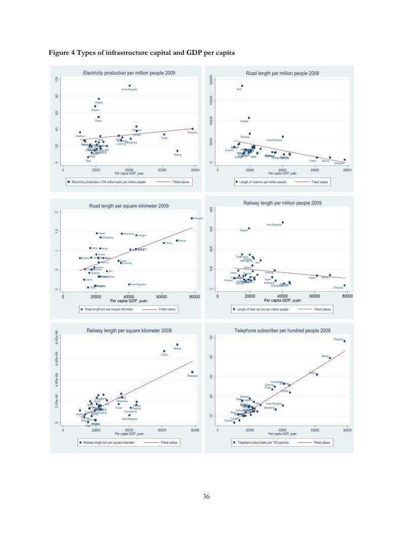
Indeed infrastructure development has altered the landscape throughout China in the last two decades.Chinese people view the ability of building such an amount of infrastructure in a short period of time as asuccess. It is not clear, however, how much infrastructure capital contribute to regional economic growth inChina. A simple set of graphs shows that the availability of infrastructure is highly correlated with thedevelopment status of the local economy. Almost all four types of infrastructure are positively correlated withthe level of per capita GDP (Figure 4 in the appendix), except that the transport infrastructure has been

13

declining with increasing migration and population growth. To answer this question, the next chapterintroduces a theoretical framework to study the direction and magnitude of such a relationship.

14

III. The Model

The model follows the usual format of a Cobb-Douglas production function. An additional capital,infrastructure, enters into the production function as Gt. The assumption is that such capital iscomplementary to private capital and that it exhibits the usual decreasing returns to scale.

Yt = (AtLt)1-α-β-γ KtαHtβGtγ (1)

where Y is real GDP, K is the stock of private physical capital, H is the stock of human capital. As in theusual Solow growth model, L is the labor, A is a labor-augmenting technology, t refers to time in years.Assume the production function exhibits constant returns to scale (CRS) for all three types of capital, whereα+β+γ<1, and decreasing returns to scale for individual capital.

Assume the labor augmenting technology At follows the path:

At = A0egtFtθ; (2)

together with Lt = L0ent (3)

where n is the population growth rate, g is the exogenous rate of technological progress, F is a measurementfor the openness of the economy. The openness variable has a positive effect on technology improvement,either through introducing more competition or through better management and technology adoption.

Assuming the accumulation of capital is in the form:

= skYt – δKt (4)

Human and infrastructure capital follow the same format with investment rate sh and sg respectively. Assumethat the depreciation rate δ is constant over time and the same for all three types of capital.

At the steady state:

y* = [skα·shβ·sgγ/(n+g+ δ)α+β+γ]1/(1-α-β-γ), where y* = Y*/AL (5)

Take natural logs on both sides of (5), and then:

ln ŷt = lnA0 +g·t + (α/1-α-β-γ)·ln [sk/(n+ g+ δ)]

+ (β/1-α-β-γ)·ln [sh/(n+ g+ δ)]

+ (γ/1-α-β-γ)·ln [sg/(n+ g+ δ)]

+ θ·lnFt where ŷt = Y/L (6)

Following Mankiw, Romer and Weil (1992), the economy approaches its steady state with a transition patharound its steady state defined by the equation:

lnyt0+h = (1 – e-ηt )lny* + e-ηt lnyt0 (7)

where η = (1-α-β-γ)(n+g+ δ).

15

Substitute lny* with equation (7) and also with lnyt = ln(Yt/AL)= ln ŷt – lnA0 –gt - θ·lnFt , and get:

lnyt0+h - lnyt0 = (1 – e-ηh ) (α/1-α-β-γ)·ln [sk/(n+ g+ δ)]

+ (1 – e-ηh ) (β/1-α-β-γ)·ln [sh/(n+ g+ δ)]

+ (1 – e-ηh ) (γ/1-α-β-γ)·ln [sg/(n+ g+ δ)]

+ (1 – e-ηh ) θ·lnFt - (1 – e-ηh ) lnyt0

+ [(1 – e-ηh ) (t0+h)g + e-ηh hg] + (1 – e-ηh ) lnA0 (8)

Therefore an estimable equation can be expressed as:

ln(yt0+h/yt0) = bk · ln [sk/(n+ g+ δ)] + bh· ln [sh/(n+ g+ δ)]

+ bg· ln [sg/(n+ g+ δ)]+bf ·lnFt +bc ·lnyt0

+ ci + at + uit (*)

where α=bk/(bk+bh+bg-bc); β=bh/(bk+bh+bg-bc); γ=bg/(bk+bh+bg-bc); θ = - bf/bc . α, β, γ are elasticities ofgrowth of real per capita GDP. The dependent variable is the difference of real GDP per capita at time twith the initial level of real GDP per capita.

Equation (*) can also be expressed in levels instead of investment rates. That is, sg can be rewritten as qt

because :

ln(sg) = ln(Gt/Lt) – ln At = ln(Gt/Lt) – (lnA0 +gt + θ·lnFt) = lnqt – (lnA0 +gt + θ·lnFt) ,

where qt is the per capita measure of a particular type of physical infrastructure stock. By simple substitutionand calculation, unrestricted form of (*) is:

ln(yt0+h/yt0) = b’k · lnsk + b’h· lnht + b’g· ln qt + bn·ln (n+ g+ δ )+ bf’ ·lnFt +bc ·lnyt0 + ci + at + uit (**)

Coefficients will be different from Equation (*). Equation (**) will be the basis of the following empiricalanalysis.

16

IV. Empirical analysis

A panel dataset of 31 of China’s provinces and municipalities covering years 1990 to 2009 is constructed totest the relationship between infrastructure and regional growth. The data are from China statistical yearbooks,sector specific yearbooks and CEIC retrieved from Chinese Academy of Social Sciences. Provincial data atthe national level statistics yearbook are reported wherever possible, because they tend to be more accuratethan provincial reports. The list of names of provinces can be found in Figure 1.

The empirical model is based on equation (**) in Part III. More specifically, the estimating equation is asfollows where qit can also be replaced by investment rate sg:

ln(yit+1_t+3/yi,t-1) = b’k· lnsik + b’h· lnhit + b’g·ln qit+ bn’·ln (ni+g+ δ )+ bf’ ·lnFit+bc·lnyi,t-1 + ci + at+ uit

(***)

i. Description of variables

Table 3 shows the list of variables used to estimate the above equation. The dependent variable is the three-year forward moving average of real GDP per capita growth expressed as ln(yit+1_t+3/yi,t-1). The objective is toeliminate the short term fluctuations in the real GDP per capita series, and to control for reverse causalitythat goes from higher real GDP per capita to more demand on infrastructure5. The regression model assumesthat the government and enterprises anticipate growth targets three years into the future to accelerateinfrastructure investment today. Whenever the paper mentions partial growth effect, growth prospect orimprovement of standard of living, it means partial effect of infrastructure capital on the three year forwardmoving average of real per capita GDP growth.

The first set of right-hand-side variables is the variables of interest Xit. The flexibility of the empirical modelallows either a stock measure or investment rates. In particular, the infrastructure variable qt. is the level ofeach type of infrastructure stock scaled by permanent population. The assumption is that it is positive andsignificant. qt can be the length of road or railway per million people, electricity production per millionpeople6, and telephone subscribers per 100 people. Private sector investment rate sit is measured by realprivate investment in fixed assets to real GDP. The human capital stock hit is measured by the share of thenumber of graduates from higher education to total permanent population for province i at time t. Theopenness variable F is measured by FDI flow per capita. It is assumed to be affecting the technologyimprovement.

Previous studies that use stock measures of infrastructure capital have encountered problems of aggregation.Hulten (1996) attempts to construct a measure of composite infrastructure stock to test the infrastructure andgrowth relationship. Zhang et al (2006) uses principle component analysis (PCA) to construct an aggregateinfrastructure capital. Calderon and Serven (2004) adopt similar approach to measure infrastructure stock fora large sample of countries. A problem with aggregation is that it can hardly give a meaningful interpretationand the results vary by the way of construction. This paper, therefore, includes the physical measures of each

5 The use of three-year forward moving average to control for possible reverse causality is also found in Devarajan et al(1996).6 Electricity production per million people is used as a proxy for the electricity generating capacity, its stock measure toavoid missing data problem. In general the more electricity generating power, the more production there will be.Regression results show that a comparison using each measure yields similar results.

17

type of infrastructure. An advantage of this is that it eliminates some endogeneity in the infrastructureinvestment process. By putting four types of infrastructure in a single equation, it studies the partial effect ofeach type of infrastructure on economic growth holding the level of other types constant..

The one year lag real per capita GDP rgdppc t-1 is included as an indicator for conditional convergence. If theprevious lagging regions have been growing at a faster rate than the previously advance regions, there isconditional convergence among the regions. The coefficient on this variable is expected to be negative.

Population is measured as permanent population. By allowing for effects of migration, it can better measurethe contribution such a population base has created and the services that it has received in that province. It isthe registered population minus the registered population that reside out of state and plus the migrationpopulation residing over six months. A time average population growth rate ni is calculated for each provincefrom 1990 to 2009. Following Mankiw, Romer and Weil (1992), Knight et al (1993), g+ δ is assumed to be0.05. The assumption is that the results are robust to changes in g+ δ. Hence the variable ngd is theadjustment by population growth, technology improvement and capital depreciation. Coefficient on thisvariable is expected to be negative.

The second set of variables is controls Zit. It includes time period and regional dummies as well as interactionterms to capture national policy change that affects sub-national performances. The dummy variables foreconomic region correspond to the Eastern, Central, Western and Northeastern regions respectively.

Time period dummies are chosen to reflect the leadership and policy changes that influence infrastructureinvestment. During the first period from 1990 to 1992, there was large and often wasteful spending oninvestment in fixed assets. The second time period is from 1993 to 1997 when the previous large amount ofinvestment began to take its toll with double digit inflation. The third time period from the year 1998 to 2002is a period when Premier Zhu Rongji initiated the reform for the SOEs and the policy endeavor usinginfrastructure investment as a fiscal stimulus. The last time period is from 2003 to the present, when thecurrent leadership in China proceeded with bold and often more flexible policies to infrastructure investment.Corresponding variables are p1 referring to years from 1993 to 1997, p2 from 1998 t 2002 and p3 from 2003to 2006, and the base period from the year1990 to 1992. Note because of the three year forward movingaverage treatment of the dependent variable, it is virtually using the data until 2006. Nonetheless it is able tocapture much of the time varying effects of infrastructure during the 17 years. Time period dummies arepreferred to year dummies because the sign and magnitude of the coefficients on year dummies are prone tochanges with different years included and some policy effects may be felt for a longer time period.

Another control is:

rdepit: the dependence ratio, measured as the sum of number of population aged from “0-14” and from “65and above” to the number of population aged from “15 to 64 years old”. This is to control for populationstructure. The assumption is that the higher the rate, the more burdensome working age population will feel.

The unobserved part consists of ci province specific effect that is constant over time, at time specific effectand the error term uit. The regression adopts the fixed effect method to eliminate the portion ci that causesendogeneity problem with the variables of interest. Robust standard errors are reported throughout to allowfor heteroskedasticity and serial correlation in the error term.

18

Table 3 Description of Variables

Variables Definitionln(RGDPPCt+1_t+3/RGDPPCt-1) Three year forward average growth rate of real per capita GDP.POP Permanent population, 10 thousand personsGRADS Share of graduates from Higher Education to permanent population (%)RDEP Real dependence ratioRSPINV Share of real private investment in fixed assets to total GDP, in 1990

pricesRFDICYPC Real FDI actually utilized, yuanln(ngd) Adjustment by population growth, technology change and capital

depreciation

ELECPDMP Electricity production (100 million kwh per million people)HWMP Length of road km per million people

RDEXPMP, RDCLIMP,RDCLIIMP,RDCLIIIMP,RDCLIVMP, RDUCMP

Length of expressway, Class I road, Class II road, Class III road, Class IVroad, and unclassified road, in km per million people

RWLENMP Length of railway km per million peopleTELESUBHP Telephone subscribers per 100 personsCELLHP Cell phone units per 100 persons

ECOZONE Eastern: 10 provinces and municipalitiesCentral: 6 provincesWestern: 12 provinces and municipalityNortheastern: 3 provinces

Time periods 1990– 19921993– 19971998– 20022003 – 2006

A problem with the data is that they are riddled with persistent nature over time and a trending behavior. Inorder to avoid running a spurious regression, augmented Dicky-Fuller unit root tests with time trend areperformed on all the variables used for estimation. The choice of lag length follows the method suggested bySchwert (1989) and the critical values follow Hamilton (1994) Table B.6. All results are based on 10% level ofsignificance. Table 4 shows the list of time series properties of the variables.

First differencing is performed on the I (1) variables, which, in the form of a natural log, becomes the growthrate of, for example, infrastructure stock. This will lose one more time period and difficulty in interpretation,as it is possible that it’s the level that affects growth of standard of living not the growth rate. In addition,variable t is included in the regression analysis to allow for an explicit trend.

19

Table 4 Time series properties of the variables

Variable Unit root TrendThe dependent variable No YesLn(RSPINV) No YesLn(RFDICYPC) No NoLn(GRADS) No YesLn(RDEP) Yes NoLn(ELECPDMP) Yes YesLn(HWMP) Yes YesLn(RDEXPMP) No NoLn(RDCLIMP)Ln(RDCLIIMP)Ln(RDCLIIIMP)Ln(RDCLIVMP)Ln(RDUCMP)

NoNoYesNoYes

NoNoYesYesYes

Ln(RWLENMP) No YesLn(TELESUBHP) No YesLn (CELLHP) No No

20

ii. Regression analysis

The purpose of this part is to interpret the results on the growth impact of infrastructure capital acrossChina’s provinces from the year 1990 to 2009. In particular, it focuses on the following questions. Hasinfrastructure contributed positively to China’s real per capita GDP growth? Do certain types ofinfrastructure have a stronger growth effect than others in certain regions and during certain time period? Hasinfrastructure played a positive role in bridging the gaps between lagging and leading regions? These questionshave particular importance for policy implications of persistent large scale infrastructure investment as inChina.

1. Average effect of infrastructure capital on China’s provincial growth

Table 5 presents the results of a first look at the impact of infrastructure capital to China’s provincial real percapita GDP growth. Equation 1.1 shows the average partial effects of the four types of infrastructure capitalon 31 China’s provinces and municipalities from 1990 to 2009. As the dataset spans a period of twenty years,the partial effects of the infrastructure capital may vary for different time periods. Results in Equation 1.2shows whether it is the case from the data. Similarly, given the diverse development background, effects ofinfrastructure capital are likely to vary for different regions. Equation 1.3 shows the partial effects of theseinfrastructure capital for four regions, Central region, Western region, Northeastern region and the referenceEastern region. The partial effect on the dependent variable can be shown in the equation: ∆ln(rgdppcf1_f3/rgdppct-1) ≈∆ (rgdppcf1_f3 – rgdppct-1)/rgdppct-1. However, to simplify the interpretation, thepartial effect will be referred to as the provincial growth effect in the context, meaning changes in the growthrate of the three year forward average of real per capita GDP.

The results from Eq. 1.1 in Table 5 are as follows. Among the four types of infrastructure, the rate ofelectricity production growth is significantly and positively related to the three year forward averages of realper capita GDP growth. Road growth in terms of per capita length has a negative growth effect. Thesignificant non-linear effect indicated by the quadratic term shows that when road per capita length growsover 44%, its effect on provincial growth will start to become positive. There are only a few cases in thesample where such high growth rates are reached. Therefore the average effect from increasing growth rate ofroad per capita length reduces real per capita GDP growth. The effects of other infrastructure capitals haveon average positive but not significant growth effect.

Eq. 1.2 shows the partial effects of road, railway and telecommunications infrastructure do vary for differenttime periods. Per capita road length growth exhibits non-linear partial effect on provincial real per capitaGDP growth. During 1990 to 1997, all road development is associated with a negative growth effect. Startingfrom the year 1998, road development exhibits a U-shape growth effect. Road development in mostprovinces is associated with a negative growth effect. Only for provinces that have a road length growthabove 35.4%, its growth effect is increasingly positive. During 2003 to 2006, however, on average roaddevelopment has a positive growth effect. Rail infrastructure has also shown a U-shape partial effect.However, given the level of railway per capita length, its growth effect has been positive throughout time.The effect of telephone ownership seems to exert a significant growth effect throughout the time period untilrecently. Telephone ownership expansion is associated with a negative growth effect. The growth effect fromincreasing electricity production, however, does not seem to vary much across time. Its partial effect ongrowth is smaller than that in Equation 1.1. One percent increase in electricity production per capita willincrease the future growth by about 0.07 percentage points.

21

Results from Eq. 1.3 show that the partial effects of infrastructure capital do differ across regions. TheEastern and Central provinces are benefiting from growth of per capita electricity production. One percentincrease in per capita electricity production growth will increase on average future growth rate of about 0.21percentage points. Electricity production per capita growth in the West, however, is associated with a muchlower growth effect. Its growth effect in the Northeastern region has even turned to negative.

The effect of road per capita length growth exerts a non-linear growth effect. On average in the Eastern,Central and Western regions additional road per capita expansion is associated with a declining growth rate offuture real per capita GDP, except for a few provinces. Road development in the Northeastern region,however, has a positive growth effect.

Railway length per capita on the other hand has on average positive but insignificant growth effect for allregions, except the Northeastern region. Additional per capita rail expansion is associated with significantnegative growth effect. The effect of telephone ownership expansion is not significant as in Eq. 1.1.

Aside from the infrastructure capital, higher foreign capital level and human capital stock are both associatedwith a higher rate of future growth as shown in Eq. 1.1. Eq. 1.2 shows that foreign capital has on average apositive growth effect throughout time. The private capital and human capital are exerting a stronger positivegrowth effect over time. Eq. 1.3 shows that for the Western and Northeastern regions growth effects ofprivate and foreign capital seem to be negative, whereas the growth effect of human capital is particularlystrong and positive.

Table 5 Average effect of infrastructure capital on real per capita economic growth

(Dependent variable: Ln(three year forward moving average of RGDPPC t+1_t+3/RGDPPCt-1); Method: fixed effects with robust standard errors)

Nationwide Nationwide bytime periods

Nationwide byregion

Eq.(1.1) Eq.(1.2) Eq.(1.3)∆Ln (ELECPDMP) 0.128** 0.0698* 0.212***

(2.14) (1.90) (2.88)

∆Ln(HWMP) -0.0910** -2.799** -0.129***

(-2.20) (-2.42) (-3.35)

[∆Ln(HWMP)]^2 0.102** 17.61** 0.141***

(2.12) (2.33) (3.04)

Ln(RWLENMP) 0.0449 0.0501** 0.0438(1.61) (2.11) (1.52)

Ln(TELESUBHP) 0.00293 0.0929*** -0.0153(0.15) (2.93) (-0.71)

Ln(RFDICYPC) 0.0212** 0.00705 0.0257***

(2.63) (0.99) (3.03)

Ln(RSPINV) 0.0346 -0.0537* 0.0276(1.70) (-1.93) (1.19)

Ln(GRADS) 0.0644*** -0.0111 0.0379(3.56) (-0.39) (1.50)

∆Ln(RDEP) 0.0116 -0.107* 0.0140(0.46) (-1.98) (0.57)

22

t 0.0387**** 0.0319**** 0.0433****

(4.73) (3.69) (5.32)

Ln(RGDPPC)t-1 -0.560**** -0.575**** -0.545****

(-7.76) (-9.11) (-7.69)

1998-2002(p2) 0.782***

(3.15)

2003-2009(p3) 1.728***

(3.47)

Ln(RGDPPC)t-1*p1 -0.0135**

(-2.29)

∆Ln(HWMP)*p1 2.541**

(2.20)

∆Ln(HWMP)*p2 2.689**

(2.31)

∆Ln(HWMP)*p3 2.748**

(2.33)

[∆Ln(HWMP)]^2*p1 -19.21**

(-2.46)

[∆Ln(HWMP)]^2*p2 -17.53**

(-2.32)

[∆Ln(HWMP)]^2*p3 -17.60**

(-2.32)

Ln(RWLENMP)*p2 -0.330***

(-2.90)

Ln(RWLENMP)*p3 -0.517**

(-2.30)

[Ln(RWLENMP)]^2*p2 0.0480***

(3.24)

[Ln(RWLENMP)]^2*p3 0.0714**

(2.46)

Ln(TELESUBHP)*p3 -0.139****

(-4.28)

Ln(RSPINV)*p2 0.0649*

(1.86)

Ln(RSPINV)*p3 0.100*

(1.97)

Ln(GRADS)*p2 0.0578**

(2.63)

Ln(GRADS)*p3 0.135***

(3.59)

∆Ln(RDEP)*p1 0.158(1.69)

∆Ln(RDEP)*p2 0.149**

23

(2.34)

∆Ln (ELECPDMP)*Western -0.182**

(-2.04)

∆Ln (ELECPDMP)*Northeastern -0.340****

(-4.36)

∆Ln(HWMP)* Northeastern 0.432***

(3.62)

[∆Ln(HWMP)]^2*Northeastern -0.613***

(-3.11)

Ln(RWLENMP)*Northeastern -0.335*

(-1.73)

Ln(RSPINV)*Northeastern -0.0483**

(-2.20)

Ln(RFDICYPC)*Northeastern -0.0367***

(-2.89)

Ln(GRADS)*Western 0.0648**

(2.11)

Ln(GRADS)*Northeastern 0.0734**

(2.29)

∆Ln(RDEP)*Northeastern -0.0922*

(-2.00)

Constant term 2.478**** 1.987**** 2.566****

(9.35) (7.68) (8.45)No. of Obs.No. of Provinces

45731

45731

45731

t statistics in parentheses*p<0.1, ** p < 0.05, *** p < 0.01, ****p < 0.001

24

2. Regional impact of infrastructure capital

The previous results show that infrastructure can play a positive role in China’s regional economic growth.Additional infrastructure investment, however, can either increase or decrease the real per capita GDPgrowth. In fact, road and railway has already shown strong signs of negative growth effect for some regionsand during some periods of time. Therefore the relevant question is to what extent infrastructure such astransport development can still be relevant in China’s provincial growth? Given the vast differences acrossChina’s regions and changing policy focuses over time, this section performs an analysis on subsamples ofeach economic region to capture the regional and time variations of the impact from infrastructure capital.

Equations 2.1 to 2.4 in Table 6 present a summary result for partial effects of infrastructure capital in each ofthe four, Eastern, Central, Western and Northeastern, regions. Since the purpose of this section is to captureboth the regional and time variation of the growth impact of infrastructure capital, it will present in a way thatcompares the partial effects across region from each type of infrastructure capital over time.

An increase in the electricity production per capita growth in the Eastern and Northeastern regions is initiallyassociated with a strong and significant growth effect. The growth effect from electricity productionexpansion in the Central and Western regions has been relatively smaller, but increasingly positive during theperiod from 1993 to 1997. Growth effect from electricity production in the Eastern region has on averagebeen positive, except for years from 1998 to 2002. Similarly for the Northeastern region, its growth effect hasbeen declining and even become negative during 1998 -2006.

Road development growth in the Eastern region has offered a very interesting scenario. Eq. 2.1 shows thatroad per capita growth in the Eastern region initially exhibits a non-linear growth effect from 1990 to 1997. Ifthe rate of road per capita growth exceeds a certain threshold, additional increase in road growth rate isassociated with higher future economic growth in the province. Below that threshold, increase in road lengthgrowth rate is associated with a decline in future growth rate. Given a sample of 12 Eastern provinces, mostprovinces have a road length growth rate that is below the threshold during the entire sample time period.From 1998 to 2002, road per capita expansion has shown to have an inverse U-shape. Road development inmost provinces is associated with a higher growth effect. A few provinces such as Jiangsu and Tianjinmunicipality are expanding roads beyond the optimal level, suggesting a too rapid road development. From2003 onward, road development again exhibits U-shape growth effect. Most provinces have experiencednegative growth effect from road expansion.

Road development in the Central and Western regions are perhaps one of the most prominent considering itsless populated area with a much higher initial road per capita length. Yet the growth effects of such expansionseem to be less desirable.

For the Central region, Eq. 2.2 shows increasing the rate of growth in road stock has a significantly negativegrowth effect from 1990 to 2002. Its negative effect, however, has become smaller over time and during theyear 2003 to 2006 has turned to a small but positive growth effect. The average rate of road network growthhas increased from – 0.1% during early 1990s to over 12% after the year 2003. Given this rate of growth inroad per capita stock comparable to the Eastern region; more roads in the Central region don’t seem to yieldstronger growth momentum as in the Eastern region.

Eq. 2.3 presents the results for Western region. Growth rate of road per capita length in the Western region isalmost zero at the beginning of 1990. During 1993 to 1997 it has increased to an average of 0.9%. Since the

25

year 1998 that initiated the Western Development Plan, road per capita length grows at about 6% annually, amuch higher rate than the early 1990s. After the year 2003, the annual road per capita growth reaches to anaverage of about 15%!

Growth effects from such skyrocketing road expansion seem to contradict to our expectations. Increasinggrowth rate of the road per capita length growth has been associated with negative growth effect since theyear 1990. Road development during the Western Development Plan doesn’t seem to provide the growthmomentum expected by the policymakers for the region. Its average growth effect is still negative andsignificant after the year 1998. From 2003 onward, with an average road per capita growth of 15%, itsnegative growth effect has become smaller, but is still significantly negative. Heavy investment in roadexpansion doesn’t seem to have a desirable effect in the West. Much of the investment may be buried in abarren land.

Growth rate of road per capita length has been increasing over time in the Northeastern region. During theinitial period, its grow rate is on average almost zero and is around 3% on average from 1998 onward. It startsto accelerate after the year 2006 to an average of 16.5%. Similarly with the Central and Western regions, Eq.2.4 shows road development in the Northeastern region has been associated with a negative growth effect onaverage. Its negative effect has been declining, yet still significantly negative in recent years.

Eq. 2.1 shows that rail expansion in the Eastern region has been positive and significant throughout the year.Rail development in the Central region has been in general favorable to its economic growth, except for theperiod between 1998 and 2002. The Western region, shown in Eq. 2.3, has seen steady increase in the growtheffect of its rail expansion. Initially rail development is associated with a negative growth effect. From the year1998 onward, rail development has been contributing more to the growth momentum of this vast and lesspopulated region. Rail development has almost zero growth effect in the Northeastern region throughout theyear. Comparing road and rail infrastructure, the Western region seems to show a contrasting scenario inrelation to economic growth.

Throughout the years, land-line telephone ownership has expanded rapidly across China’s regions. Table 6shows that its growth effect in the Eastern is positive but not significant from the year 1990 to 2002.Afterwards, additional telephone ownership has been associated with a declining growth effect. The Westernregion also enjoys a positive and significant growth effect initially. From the year 2003 onward, its growtheffect has turned to negative and significant. Northeastern region has benefited from telephonepopularization during 1993 to 2002, whereas in other years, its growth effect is negative. One possible reasonto explain the declining role of telephone ownership to growth is that its role has been gradually replaced bythe introduction of cell phone. It is particularly true in the latter half of the time period. The effect of cellphone usage will be discussed in the following chapter that may explain the lessening effect of telephone.

26

Table 6 Regional impact of infrastructure capital(Dependent variable: Ln (three year forward moving average of RGDPPC t+1_t+3/RGDPPCt-1); Method: fixed effects with robust standard errors)

Eastern Central Western NortheasternEq.(2.1) Eq.(2.2) Eq.(2.3) Eq.(2.4)

Ln(RGDPPC)t-1 -0.611**** -0.897**** -0.108 -0.778*

(-10.79) (-12.86) (-0.58) (-4.18)

∆Ln (ELECPDMP) 0.365** -0.0430 -0.695**** 0.863**

(3.03) (-0.75) (-11.03) (5.73)

∆Ln(HWMP) -9.750**** -5.592* -0.0737* -2.861***

(-4.85) (-2.55) (-2.00) (-30.33)

[∆Ln(HWMP)]^2 61.66***

(4.50)

Ln(RWLENMP) 0.0501*** 0.146*** -0.164*** 0.00412(3.47) (4.49) (-4.10) (0.03)

Ln(TELESUBHP) 0.0148 0.108** 0.137** -0.180*

(0.28) (3.54) (2.83) (-3.43)

Ln(RFDICYPC) -0.00673 0.0283*** -0.00655 0.0233(-0.29) (6.63) (-0.82) (1.99)

Ln(RSPINV) -0.0986** 0.104** 0.111*** -0.138**

(-2.43) (2.84) (3.30) (-5.26)

Ln(GRADS) 0.0699* 0.177* -0.0698* 0.00987(2.19) (2.22) (-1.85) (0.22)

∆Ln(RDEP) -2.270*** 0.0953 0.166*** -0.0904(-4.21) (1.62) (3.32) (-0.83)

t 0.0560** 0.0434** 0.0285 0.0673**

(3.14) (3.42) (1.44) (6.19)

1993-1997(p1) 1.106***

(4.03)

1998-2002(p2) 1.186**** -0.488**

(5.65) (-2.72)

2003-2009(p3) 0.332 -3.049*** 1.018**

(1.82) (-5.75) (8.46)

Ln(RGDPPC)t-1*p1 -0.133** -0.340****

(-3.22) (-6.29)

Ln(RGDPPC)t-1*p2 -0.413****

(-7.01)

Ln(RGDPPC)t-1*p3 0.422** -0.196(3.78) (-2.18)

∆Ln (ELECPDMP)*p1 0.378* 0.722**** -0.665***

(2.34) (6.28) (-17.87)

∆Ln (ELECPDMP)*p2 -0.383* 0.711**** -0.883**

(-1.90) (9.20) (-6.89)

∆Ln (ELECPDMP)*p3 0.731*** -0.968*

27

(3.24) (-4.19)

∆Ln(HWMP)*p1 9.605**** 5.147*

(4.90) (2.34)

∆Ln(HWMP)*p2 9.867**** 5.538 2.836****

(4.93) (2.55) (32.47)

∆Ln(HWMP)*p3 9.733**** 5.693** 0.0586 2.773***

(4.97) (2.62) (1.21) (27.83)

[∆Ln(HWMP)]^2*p1 -63.80***

(-4.70)

[∆Ln(HWMP)]^2*p2 -61.82***

(-4.51)

[∆Ln(HWMP)]^2*p3 -61.63***

(-4.52)

Ln(RWLENMP)*p1 -0.163** 0.146****

(-3.33) (8.55)

Ln(RWLENMP)*p2 -0.558**** 0.310****

(-5.11) (9.52)

Ln(RWLENMP)^2*p2 0.0819****

(4.83)

Ln(RWLENMP)*p3 0.376****

(8.65)

Ln(TELESUBHP)*p1 -0.0489* 0.204**

(-2.12) (5.83)

Ln(TELESUBHP)*p2 -0.0794** 0.185**

(-2.30) (6.71)

Ln(TELESUBHP)*p3 -0.0893* -0.492****

(-1.89) (-5.75)

Ln(RSPINV)*p1 0.134*** -0.181** -0.199*** 0.253***

(3.47) (-3.25) (-4.33) (16.72)

Ln(RSPINV)*p2 0.137*** -0.122*** 0.103***

(3.53) (-3.18) (16.58)

Ln(RSPINV)*p3 -0.280**** -0.106** 0.397***

(-7.72) (-2.92) (29.90)

Ln(RFDICYPC)*p1 0.0776*** -0.0714***

(3.63) (-15.11)

Ln(RFDICYPC)*p2 0.0667** -0.0740***

(2.58) (-13.64)

Ln(RFDICYPC)*p3 0.0643** -0.0607**

(2.72) (-6.19)

Ln(GRADS)*p1 0.101*** -0.222**

(4.08) (-7.62)

Ln(GRADS)*p2 -0.0815** -0.114* 0.170****

(-2.66) (-2.07) (4.63)

28

Ln(GRADS)*p3 -0.231** 0.235**** -0.154(-3.28) (9.46) (-2.41)

∆Ln(RDEP)*p1 2.225***

(3.92)

∆Ln(RDEP)*p2 2.254*** -0.174(3.99) (-1.70)

∆Ln(RDEP)*p3 2.340*** 0.194(4.62) (1.29)

Constant term 2.500**** 3.812**** 1.535*** 2.768(10.52) (8.07) (3.31) (1.68)

No. of Obs.No. of Provinces

15110

966

16212

483

t statistics in parentheses*p<0.1, ** p < 0.05, *** p < 0.01, ****p < 0.001

3. The catching up process

Figure 2 shows that China’s provinces are diverging, where a greater share of GDP has been enjoyed by asmaller share of population in leading provinces. This part again visits the issue to see whether there isevidence of conditional convergence among the provinces. Given the neoclassical growth model introducedin the previous chapter, the coefficient on the lagged term of real per capita GDP is expected to be negativeto if there is evidence of conditional convergence among provinces. This shows that lagging provinces whichhave a lower initial level of economic development will grow faster and eventually catch up with otherprovinces.

Equations 1.1 to 1.3 in Table 5 show there is evidence of conditional convergence among all provinces acrossthe country. Equations 2.1 to 2.4 present further evidence that such conditional convergence is felt by all fourregions. If considering both time and regional varying effects, Eq. 3 and Eq. 4 in Table 9 show that bothrandom effect and fixed effect methods yield similar results in terms of the catching up process. Randomeffect estimation shows that the catching up process is faster in particular for the Central region throughouttime. The catching up process slows down and there are signs of diverging after the year 2003 in the randomeffect estimation. The effects from the fixed effect estimation, however, show a much stronger catching upprocess. Considering possible correlation between the explanatory variables and the unobservedheterogeneity, the results from the fixed effect approach seems to be more appropriate.

4. Marginal effects of an increase in infrastructure network

In order to compare the regional and time effect of different infrastructure capital, this section envisages theeffect of a marginal increase in either the growth rate or the stock of a particular type of infrastructure capital.The purpose of this section is to present a more concrete example of the effect of infrastructure capital onregional growth. What type of infrastructure has played a more important role in promoting and facilitatingeconomic growth? What type of infrastructure still has the potential to drive the regional economy?

29

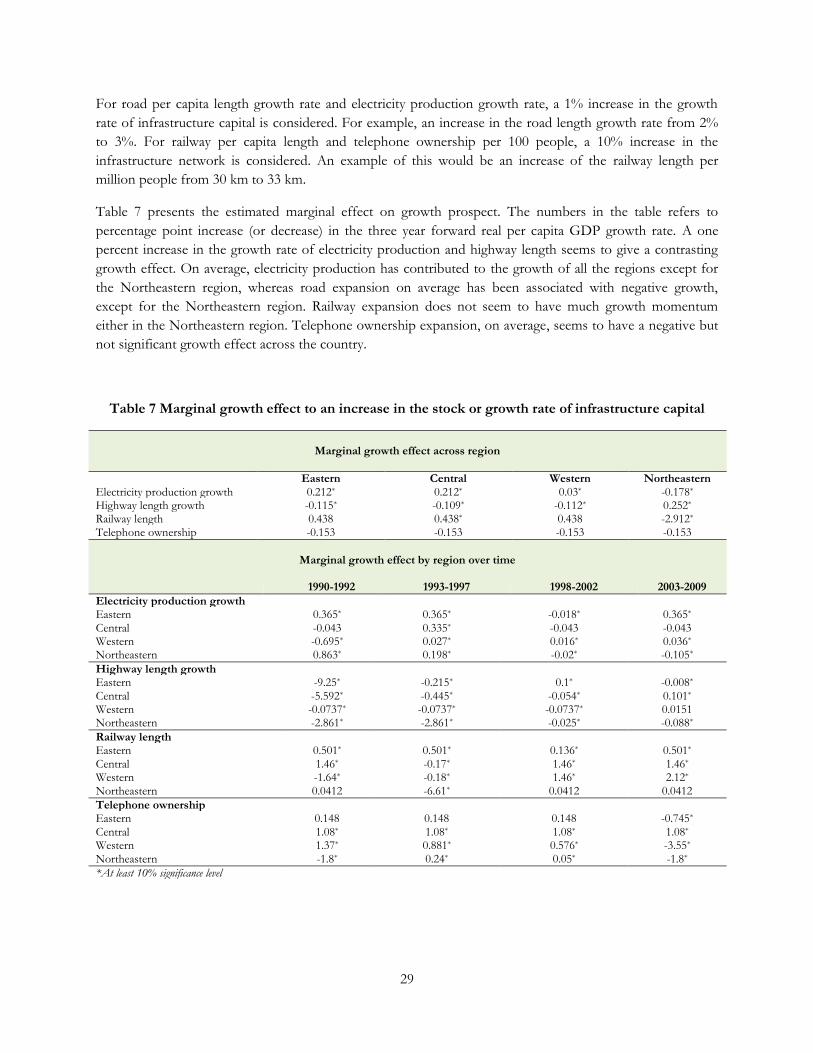
For road per capita length growth rate and electricity production growth rate, a 1% increase in the growthrate of infrastructure capital is considered. For example, an increase in the road length growth rate from 2%to 3%. For railway per capita length and telephone ownership per 100 people, a 10% increase in theinfrastructure network is considered. An example of this would be an increase of the railway length permillion people from 30 km to 33 km.

Table 7 presents the estimated marginal effect on growth prospect. The numbers in the table refers topercentage point increase (or decrease) in the three year forward real per capita GDP growth rate. A onepercent increase in the growth rate of electricity production and highway length seems to give a contrastinggrowth effect. On average, electricity production has contributed to the growth of all the regions except forthe Northeastern region, whereas road expansion on average has been associated with negative growth,except for the Northeastern region. Railway expansion does not seem to have much growth momentumeither in the Northeastern region. Telephone ownership expansion, on average, seems to have a negative butnot significant growth effect across the country.

Table 7 Marginal growth effect to an increase in the stock or growth rate of infrastructure capital

Marginal growth effect across region

Eastern Central Western NortheasternElectricity production growth 0.212* 0.212* 0.03* -0.178*

Highway length growth -0.115* -0.109* -0.112* 0.252*

Railway length 0.438 0.438* 0.438 -2.912*

Telephone ownership -0.153 -0.153 -0.153 -0.153

Marginal growth effect by region over time

1990-1992 1993-1997 1998-2002 2003-2009Electricity production growthEastern 0.365* 0.365* -0.018* 0.365*

Central -0.043 0.335* -0.043 -0.043Western -0.695* 0.027* 0.016* 0.036*

Northeastern 0.863* 0.198* -0.02* -0.105*

Highway length growthEastern -9.25* -0.215* 0.1* -0.008*

Central -5.592* -0.445* -0.054* 0.101*

Western -0.0737* -0.0737* -0.0737* 0.0151Northeastern -2.861* -2.861* -0.025* -0.088*

Railway lengthEastern 0.501* 0.501* 0.136* 0.501*

Central 1.46* -0.17* 1.46* 1.46*

Western -1.64* -0.18* 1.46* 2.12*

Northeastern 0.0412 -6.61* 0.0412 0.0412Telephone ownershipEastern 0.148 0.148 0.148 -0.745*

Central 1.08* 1.08* 1.08* 1.08*

Western 1.37* 0.881* 0.576* -3.55*

Northeastern -1.8* 0.24* 0.05* -1.8*

*At least 10% significance level

30

Table 7 also presents the projection of a marginal change in the four types of infrastructure capital. Themarginal change discussed here is either a 1% increase in the growth rate of a type of capital or a 10%increase in the stock of a type of capital.

Increase in the electricity production growth rate has in general a strong growth effect in the Eastern regioncompared with other regions, except for the years from 1998 to 2002. Electricity infrastructure investmentseems to play an increasing role in the regional development of the Western provinces. A marginal increase inthe growth rate of electricity production per capita is initially associated with a reduction in the growth of percapita GDP. Over time its growth effect has turned to positive, although not as strong as that for the Easternregion. The Northeastern region, on the other hand, has seen a gradually decreasing role of the electricityinfrastructure. A marginal increase in electricity production per capita has contributed less to the provincialgrowth over time. Its growth effect has even turned to negative in the latter half of the time period. Electricityinfrastructure in the Central region has on average played a minimum role, except during the year 1993 to1997.

Road infrastructure growth has in general a negative growth effect to the provincial real per capita GDP forthe Eastern and Northeastern regions, except for the period from 1998 to 2002 in the Eastern region. Therole of road infrastructure to economic growth in the Central region seems to be increasing. Roadinfrastructure investment in the Western region has seen a persistent reduction to its provincial growth. Itsgrowth effect has turned to positive but insignificant in recent years.

Railway infrastructure investment has boded well in general for the Eastern and Central regions, exceptduring the year 1993 to 1997 for the Central region. Railway infrastructure has becoming more important forthe Western region. Its network expansion initially has a negative growth effect. Its growth effect has turnedto positive in the latter half of the time period. Railway development seems to have a negligible growth effectfor the Northeastern region, except that its growth effect has become very negative during 1993 to 1997.

Telephone infrastructure has contributed positively to the provincial growth in Eastern and Western regionsuntil recently. Its growth effects have become negative for both regions after the year 2003. Telephoneinfrastructure investment seems to benefit the Central region on average, whereas its growth effect fluctuatesover time for the Northeastern region.

The above results projected have several implications for regional economic development in China. First,electricity infrastructure investment drives the energy-demanding Eastern region and the Western regionwhere it has abundant energy resources and energy producers. Second, consistent rapid growth in roadinfrastructure investment does not seem to provide further growth momentum to its regional economicgrowth. Rather such large investment scale has diverted resources that would be more productive in otherareas. Railway development, on the other hand, seems to have more growth potential for the Eastern, Centraland Western regions, in particular for the West. Perhaps in the Western area, building railway capacity is morecompatible to the industrial sectors than building roads that few people tread. Third, the role of telephoneinfrastructure has gradually been declining. Alternative investment may yield higher growth effect. This isfurther discussed in the alternative model specification including cell phone development in the next section.

Infrastructure investment enhances production capacity and in itself creates employment which can boostprovincial growth. It can also complement the growth of production in other sectors by reducing productioncost or adjustment coast, as shown in electricity production and railway development in some regions.Infrastructure investment, however, does not always yield desirable results. There is evidence of

31

overinvestment in certain types of infrastructure capital, such as road. Contrary to our conventional wisdom,road does not seem to lead to prosperity. Road that leads to nowhere can only divert valuable resources frommore productive sectors.

32

iii Alternative specifications and results

1. Endogenous investment decision

Previous results are based on the assumption that private and foreign entities make their investment decisionstaking infrastructure capital as given. A more realistic situation is that a better investment climate oftenencourages expansion of private and foreign investment, because of lower cost of transportation and otherinfrastructure services. For example, see a discussion on the private adjustment cost from Anderson et al(2006). A simple way of testing is to include interaction terms of infrastructure with private or foreigninvestments. The aforementioned infrastructure capital variables are demeaned to show the marginal effect ofFDI or private capital with infrastructure above the national average level. Table 8 shows the results of theendogenous investment using this simple test.

The growth effect of real private capital is much greater in provinces where the telephone ownership exceedsthe national average, suggesting the benefit of telephone communications to productivity enhancement andmobilization of the people. The growth effect of real private capital is also stronger for provinces with ahigher than average railway network per million people. Its effect, however, is lower for regions with a higherthan average road network per million people. Road network expansion seems to divert economic activitiesrather than attracting more private capital.

Road length per million people above the average level will enhance the positive effect of FDIs, whereashigher electricity production per million people will lower the contribution of FDI. Perhaps foreign directinvestment is more concentrated in provinces with more manufacturing sector than the energy sector.

Table 8 Impact of infrastructure capital with endogenous investment

(Dependent variable: Ln(three year forward moving average of RGDPPC t+1_t+3/RGDPPCt-1); Method: fixed effects with robust standard errors)

Ln(RGDPPC)t-1 -0.535****

(-7.49)

Ln(RSPINV)*tele0 0.0506***

(3.27)

Ln(RSPINV)*hw0 -0.0419**

(-2.54)

Ln(RSPINV)*rw0 0.0520**

(2.09)

Log(RFDICYPC)*elep0 -0.0300****

(-4.41)

Ln(RFDICYPC)*hw0 0.0151**

(2.40)

∆Ln (ELECPDMP) 0.0600(1.64)

∆Ln(HWMP) -0.0310(-1.09)

Ln(RWLENMP) 0.194***

(2.83)

33

Ln(TELESUBHP) 0.0173(0.82)

Ln(RFDICYPC) 0.00308(0.71)

Ln(RSPINV) -0.00670(-0.40)

Ln(GRADS) 0.0810****

(4.63)

∆Ln(RDEP) -0.0310(-1.23)

t 0.0337****

(4.38)

Constant term 1.671****

(3.77)No. of Obs.No. of Provinces

45731

t statistics in parentheses*p<0.1, ** p < 0.05, *** p < 0.01, ****p < 0.001

2. Road classifications and cell-phone usage

The objective of modern transportation development gradually shifts from road connectivity to the speed andquality of travel. High speed train, subway and higher quality expressway are all examples of the currenttransportation development in China. It is therefore, interesting to explore whether the quality and speed oftransportation contributes to the provincial growth. Given data limitation, a regression with a smaller samplefrom 1999 to 2009 is performed with roads of detailed classifications (Table 10).

The development of Class III and IV roads may exert a negative growth effect, although such effect is notsignificant on average. Expressway development seems to yield a much stronger growth impact in theWestern region, whereas its effect on the other regions may actually be negative. Developing Class I and IIroads has a strong positive growth effect for the Northeastern region.

Telecommunications development shows that the more mobile the population the less desirable a telephoneownership would be. In fact cell phone ownership has a strong positive growth effect, replacing the effect oftelephone. Such effect is particularly evident in the Central region, but negative for Northeastern provinces.

34

V. Conclusions

This paper investigates the relationship between infrastructure capital and economic growth in China’sprovinces. The results show that infrastructure has a positive role to play in China’s regional economicgrowth. This is particularly evident in the analysis of the electricity and railway infrastructure for the laggingregions.

The findings of the paper, however, also yield what, at first glance, seem very surprising results. Moreinfrastructure capital is not always better. China’s provinces have already shown strong evidence of investingtoo fast in road infrastructure. This is particularly true for the Western regions, which are often the recipientsof large central transfers and favorable credits for infrastructure projects. Such results reveal a remarkabletruth that infrastructure when invested beyond a proper level or speed can be detrimental economic growth.This result contrasts many studies that conclude with a policy recommendation for more roads in theWestern and Central regions.

These empirical findings should not be so surprising from a theoretical perspective. There is a limit to thegrowth effect of infrastructure capital in general and more public infrastructure may actually crowd-outprivate capital. Thus seemingly productive infrastructure investment may become unproductive if there is anexcessive amount of them. It, however, seriously questions the conventional wisdom that road developmentlead to prosperity. A large resource waste from building roads can lead to nowhere.

This conclusion, however, cannot be over-interpreted as there should be a specific level of infrastructureinvestment. Instead it shows that there is a level of infrastructure investment that’s comparable to the level ofdevelopment. Any type of infrastructure, if investing beyond the current economic conditions will bedetrimental. A certain level of infrastructure may become favorable to growth again if there is a demand. Forexample large amount of road investment may solve the bottlenecks in the urbanization of China’smetropolitan areas and speed up growth. In addition, infrastructure development may come out of an equityconcern in the public investment decision making.

If the empirical findings discussed can hold with further scrutiny, they will have important policy implications.The recommendation for more road infrastructure in lagging regions may be misleading. Spending too muchon building roads may not be a better option than developing the energy or railway sector.

These findings open up new questions for further research. What are the economic explanations for sub-national governments to invest too much in public infrastructure? How much effect infrastructure spendingcan be and continue to be an effective tool of fiscal stimulus, as it is often the case during possible economicdownturn? The results from more rigorous methods may better support the findings. Considering theinteraction between private investment, FDI and infrastructure spending in a simultaneous equation modeland a GMM approach may yield additional support to the conclusions here.

The results in this paper also contribute to the recent effort to empirically test the neoclassical economicgrowth model. By exploring the diversity of China’s growth experience, the findings support the role offoreign, human, private capital investment and its relation to infrastructure.

35

APPENDIX

Figure 3 Map of China

36

Figure 4 Types of infrastructure capital and GDP per capita

Anhui

BeijingChongqing

Fujian

GansuGuangdong

Guangxi

Guizhou

Hainan

HebeiHenanHeilongjiang

Hubei

Hunan

Inner Mongolia

Jiangsu

Jiangxi

Jilin

Liaoning

Ningxia

Qinghai

Sichuan

Shanghai

Shandong

Shanxi

Shannxi

Tibet

Tianjin

XinjiangYunnan

Zhejiang

020

4060

8010

0

0 20000 40000 60000 80000Per capita GDP, yuan

Electricity production (100 million kwh) per million people Fitted values

Electricity production per million people 2009

Anhui

Beijing

Chongqing

Fujian

Gansu

GuangdongGuangxi

Guizhou

Hainan HebeiHenan

HeilongjiangHubei

Hunan

Inner Mongolia

Jiangsu

Jiangxi JilinLiaoning

Ningxia

Qinghai

Sichuan

Shanghai

Shandong

ShanxiShannxi

Tibet

Tianjin

Xinjiang

Yunnan

Zhejiang

050

0010

000

1500

020

000

0 20000 40000 60000 80000Per capita GDP, yuan

Length of road km per million people Fitted values

Road length per million people 2009

Anhui

BeijingChongqing

Fujian

Gansu

Guangdong

Guangxi

Guizhou

Hainan

Hebei

Henan

Heilongjiang

Hubei

Hunan

Inner Mongolia

Jiangsu

Jiangxi

Jilin

Liaoning

Ningxia

Qinghai

Sichuan

Shanghai

Shandong

Shanxi

Shannxi

Tibet

Tianjin

Xinjiang

Yunnan

Zhejiang

0.5

11.

52

0 20000 40000 60000 80000Per capita GDP, yuan

Road length km per square kilometer Fitted values

Road length per square kilometer 2009

Anhui

Beijing

ChongqingFujian

Gansu

Guangdong

GuangxiGuizhou Hainan

Hebei

Henan

Heilongjiang

HubeiHunan

Inner Mongolia

Jiangsu

Jiangxi

Jilin

Liaoning

Ningxia

Qinghai

SichuanShanghai

Shandong

Shanxi

Shannxi

Tibet

Tianjin

Xinjiang

Yunnan

Zhejiang

010

020

030

040

0

0 20000 40000 60000 80000Per capita GDP, yuan

Length of total rail, km per million people Fitted values

Railway length per million people 2009

Anhui

Beijing

Chongqing Fujian

Gansu

GuangdongGuangxiGuizhou Hainan

HebeiHenan

HeilongjiangHubeiHunan

Inner Mongolia

JiangsuJiangxiJilin

Liaoning

Ningxia

QinghaiSichuan

Shanghai

ShandongShanxi

Shannxi

Tibet

Tianjin

Xinjiang

Yunnan

Zhejiang

02.

00e-

064.

00e-

066.

00e-

068.

00e-

06

0 20000 40000 60000 80000Per capita GDP, yuan

Railway length km per square kilometer Fitted values

Railway length per square kilometer 2009

Anhui

Beijing

Chongqing

Fujian

Gansu

Guangdong

Guangxi

Guizhou

HainanHebei

Henan

Heilongjiang

HubeiHunan

Inner Mongolia

Jiangsu

Jiangxi

Jilin

Liaoning

Ningxia

Qinghai

Sichuan

Shanghai

ShandongShanxiShannxi

Tibet

Tianjin

Xinjiang

Yunnan

Zhejiang

1020

3040

50

0 20000 40000 60000 80000Per capita GDP, yuan

Telephone subscribers per 100 persons Fitted values

Telephone subscriber per hundred people 2009

37

Table 9 Average effect of infrastructure capital on real per capita economic growth

(Dependent variable: Log(three year forward moving average of RGDPPC t+1_t+3/RGDPPCt-1); Method: fixed or random effects with robust standard errors)

RE FEEq.(3) Eq.(4)

Ln(RGDPPCt-1) -0.125**** -0.578****

(-3.51) (-6.84)

∆Ln (ELECPDMP) 0.139** 0.0836*

(2.39) (2.02)

∆Ln(HWMP) -1.375* -0.564***

(-1.90) (-3.47)

Ln(RWLENMP) -0.0377** -0.00311(-2.39) (-0.11)

Ln(TELESUBHP) 0.0621*** 0.0388*

(2.78) (1.77)

Ln(RFDICYPC) 0.0237*** 0.0371***

(3.27) (3.06)

Ln(RSPINV) -0.0112 -0.0333(-0.50) (-1.25)

Ln(GRADS) 0.0533*** 0.00734(2.58) (0.34)

Ln(ngd) -0.185****

(-3.93)

∆Ln(RDEP) -0.487 -0.0565(-1.33) (-1.16)

Ln(LAND) 0.0163***

(2.78)

t -0.00571 0.0422****

(-1.01) (4.87)

1993-1997(p1) -0.255****

(-3.36)

2003-2009(p3) -0.582***

(-2.60)

Ln(RGDPPCt-1)*p3 0.147***

(2.62)

Ln(RGDPPCt-1)*Central -0.0496**

(-2.46)

∆Ln (ELECPDMP)*Central 0.264**

(2.49)

∆Ln (ELECPDMP)*Western -0.119 -0.0378(-1.55) (-0.55)

∆Ln (ELECPDMP)*Northeastern -0.202**** -0.186**

(-3.36) (-2.68)

38

∆Ln(HWMP)*p1 1.377*

(1.89)

∆Ln(HWMP)*p2 1.317* 0.525***

(1.83) (3.10)

∆Ln(HWMP)*p3 1.342* 0.588***

(1.88) (3.40)

Ln(RWLENMP)*p2 -0.212**** 0.0574***

(-5.99) (3.03)

Ln(RWLENMP)*p3 0.0598** 0.102****

(2.51) (3.67)

Ln(RWLENMP)^2*p2 0.0344****

(5.83)

Ln(RWLENMP)*Central 0.0603*** 0.0922**

(3.28) (2.36)

Ln(RWLENMP)*Northeastern -0.0247**** -0.586****

(-6.13) (-4.35)

Ln(TELESUBHP)*p2 0.0369(1.63)

Ln(TELESUBHP)*p3 -0.178**** -0.0848****

(-3.78) (-4.28)

Ln(TELESUBHP)*Central -0.0427*

(-1.69)

Ln(TELESUBHP)*Northeastern -0.0622****

(-3.82)

Ln(RFDICYPC)*p1 -0.0358**

(-2.53)

Ln(RFDICYPC)*p2 -0.0249**

(-2.24)

Ln(RFDICYPC)*Central -0.0241**

(-2.08)

Ln(RFDICYPC)*Western -0.0202(-1.26)

Ln(RSPINV)*p1 0.0159**

(2.49)

Ln(RSPINV)*p2 0.0468**

(2.11)

Ln(RSPINV)*Central 0.0781***

(3.26)

Ln(RSPINV)*Western 0.0393****

(4.89)

Ln(GRADS)*p2 0.0564***

(3.53)

Ln(GRADS)*p3 0.0830***

39

(2.95)

∆Ln(RDEP)*p1 0.616*

(1.66)

∆Ln(RDEP)*p2 0.606*

(1.67)

∆Ln(RDEP)*p3 0.534(1.47)

∆Ln(RDEP)*Central 0.130(1.67)

∆Ln(RDEP)*Western 0.149**

(2.32)

∆Ln(RDEP)*Northeastern -0.245****

(-4.12)

Central*p1 0.122**** 0.0604**

(3.85) (2.48)

Central*p2 0.147***

(2.77)

Central*p3 0.198***

(3.06)

Western*p3 0.130****

(4.13)

Northeastern*p2 -0.0515(-1.50)

Northeastern*p3 0.0994**

(2.23)

Constant term 0.539** 2.606****

(2.02) (8.37)No. of Obs.No. of Provinces

45731

45731

t statistics in parentheses*p<0.1, ** p < 0.05, *** p < 0.01, ****p < 0.001

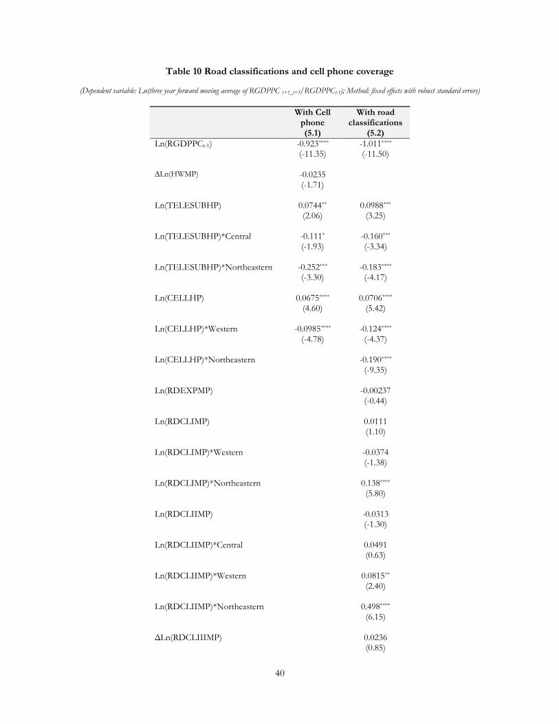
40

Table 10 Road classifications and cell phone coverage

(Dependent variable: Ln(three year forward moving average of RGDPPC t+1_t+3/RGDPPCt-1); Method: fixed effects with robust standard errors)

With Cellphone

With roadclassifications

(5.1) (5.2)Ln(RGDPPCt-1) -0.923**** -1.011****

(-11.35) (-11.50)

∆Ln(HWMP) -0.0235(-1.71)

Ln(TELESUBHP) 0.0744** 0.0988***

(2.06) (3.25)

Ln(TELESUBHP)*Central -0.111* -0.160***

(-1.93) (-3.34)

Ln(TELESUBHP)*Northeastern -0.252*** -0.183****

(-3.30) (-4.17)

Ln(CELLHP) 0.0675**** 0.0706****

(4.60) (5.42)

Ln(CELLHP)*Western -0.0985**** -0.124****

(-4.78) (-4.37)

Ln(CELLHP)*Northeastern -0.190****

(-9.35)

Ln(RDEXPMP) -0.00237(-0.44)

Ln(RDCLIMP) 0.0111(1.10)

Ln(RDCLIMP)*Western -0.0374(-1.38)

Ln(RDCLIMP)*Northeastern 0.138****

(5.80)

Ln(RDCLIIMP) -0.0313(-1.30)

Ln(RDCLIIMP)*Central 0.0491(0.63)

Ln(RDCLIIMP)*Western 0.0815**

(2.40)

Ln(RDCLIIMP)*Northeastern 0.498****

(6.15)

ΔLn(RDCLIIIMP) 0.0236(0.85)

41

ΔLn(RDCLIIIMP)*Western -0.0243(-0.67)

ΔLn(RDCLIIIMP)*Northeastern -0.169****

(-4.02)

Ln(RDCLIVMP) 0.0297*

(1.77)

Ln(RDCLIVMP)*Central -0.0229(-0.82)

Ln(RDCLIVMP)*Western -0.0417(-1.21)

Ln(RDCLIVMP)*Northeastern -0.0491(-1.28)

ΔLn(RDUCMP) -0.0189****

(-4.13)

ΔLn(RDUCMP)*Western 0.0183*

(2.04)

ΔLn(RDUCMP)*Northeastern 0.0290***

(3.04)

∆Ln (ELECPDMP) -0.0176 -0.0482**

(-0.87) (-2.29)

∆Ln (ELECPDMP)*Central 0.0319(0.60)

∆Ln (ELECPDMP)*Western 0.0485(1.15)

∆Ln (ELECPDMP)*Northeastern 0.228****

(5.72)

Ln(RWLENMP) 0.0196 0.000529(0.98) (0.03)

Ln(RWLENMP)*Central 0.178**** 0.183***

(4.43) (3.31)

Ln(RWLENMP)*Northeastern -0.578*** -0.495****

(-3.03) (-4.60)

Ln(RGDPPCt-1)*Central 0.194** 0.343***

(2.06) (2.91)

Ln(RGDPPCt-1)*Westerb 0.630**** 0.646****

(8.33) (6.90)

Ln(RFDICYPC) 0.0152** 0.0220**

42

(2.15) (2.20)

Ln(RFDICYPC)*Western -0.0211** -0.0270(-2.14) (-1.59)

Ln(RSPINV) 0.119**** 0.0854****

(6.99) (5.25)

Ln(RSPINV)*Western -0.0541**

(-2.14)

Ln(GRADS) 0.0894*** 0.0678**

(3.54) (2.58)

Ln(GRADS)*Northeastern 0.164***

(3.25)

ΔLn(RDEP) -0.0143 0.0516(-0.59) (1.55)

ΔLn(RDEP)*Northeastern 0.240**

(2.58)

t 0.0164 0.0277*

(1.43) (1.89)

Ln(RFDICYPC)*Central -0.0218(-1.32)

ΔLn(RDEP)*Central -0.145**

(-2.36)

ΔLn(RDEP)*Western -0.0675(-1.22)

Constant term 3.514**** 3.171****

(11.02) (9.01)No. of Obs.No. of Provinces

23931

22730

t statistics in parentheses*p<0.1, ** p < 0.05, *** p < 0.01, ****p < 0.001

43

REFERENCES:

Anderson, Edward, Paolo de Renzio and Stephanie Levy (2006), “The Role of Public Investment in PovertyReduction: Theories, Evidence and Methods”, Overseas Development Institute Working Paper 263.

Aschauer, David Alan (1989a), “Does Public Capital Crowd Out Private Capital”, Journal of MonetaryEconomics 24, 171-188.

Aschauer, David Alan (1989b), “Is Public Expenditure Productive?” Journal of Monetary Economics 23, 177-200.

Bai, Chong-En and Yingyi Qian (2010), “Infrastructure development in China: The cases of electricity,highways, and railways”, Journal of Comparative Economics 38, pp34-51.

Calderon, Cesar, Serven, Luis (2004), “The Effects of Infrastructure Development on Growth and IncomeDistribution”, Policy Research Working Paper Series No. 3400, The World Bank.

China Statistical Yearbook, various issues.

Devarajan, Shantayanan, Swaroop, Vinaya and Zou, Heng-fu (1996), “The Composition of PublicExpenditure and Economic Growth”, Journal of Monetary Economics 37, 313-344.

Demurger, Sylvie (2001), “Infrastructure Development and Economic Growth: An Explanation for RegionalDisparities in China”, Journal of Comparative Economics, 29, pp. 95 – 117.

Fan, Shenggen, Xiaobo Zhang, Linxiu Zhang and Jikun Huang (2004), “Local Governance and Public GoodsProvision in Rural China”, Journal of Public Economics, 88, pp 2857-2871.

Fisher, Ronald (1997), “The Effect of State and Local Public Services on Economic Development”, NewEngland Economic Review, Mar., pp53-82.

Hamilton, J. (1994). Time Series Analysis. Princeton University Press, New Jersey.

Hirschman, Albert O. (1957), “Economic Policy in Underdeveloped Countries”, Economic Developmentand Cultural Change, Vol. 5, No. 4, pp. 362 – 370.

Holtz-Eakin, Douglas and Amy E. Schwartz (1994), “Public Sector Capital and the Productivity Puzzle,” TheReview of Economics and Statistics, Vol. 76, No. 1, pp12-21.

Hulten, Charles R. (1996), “Infrastructure Capital and Economic Growth: How Well You Use it May BeMore Important than How Much You Have,” NBER Working paper 5847.

Knight, Malcolm, Norman Loayza and Delano Villanueva (1993), “Testing the Neoclassical Theory ofEconomic Growth,” IMF Staff Papers Vol. 40, No.3, The International Monetary Fund.

44

Mankiw N. Gregory, David Romer and David N. Weil (1992), “A Contribution to the Empirics of EconomicGrowth”, The Quarterly Journal of Economics, Vol. 107, No. 2, pp407-437.

Nurkse, Ragnar (1952), “Some International Aspects of the Problem of Economic Development”, AmericanEconomic Review, Vol. 42, No. 2 Papers and the Proceedings of the Sixty-fourth Annual Meeting of theAmerican Economic Association, pp. 571 – 583.

Rosenstein-Rodan, Paul N. (1943), “Problems of Industrialization of Eastern and South-Eastern Europe”,Economic Journal, Vol. 53, No. 210/211, pp. 202 -211.

Schwert, W. (1989), “Test for Unit roots: A Monte Carlo Investigation,” Journal of Business and EconomicStatistics, 7, pp.147-159.

World Development Report (1994). Infrastructure for Development. World Bank, Oxford University Press.

The World Bank, (1995), “China: Public Investment and Finance”, World Bank Report No. 14540-CHA.

Zhang, Jun, Yong Bo, Yuan Gao and Hong Zhang (2007), “Elementary Study on China’s State ofInfrastructure: Decentralization, Governance and the Determination of Infrastructure. The EconomicsReview (in Chinese), 3, pp4-19.