the road to identifying disease causing genes: association
TRANSCRIPT

THE ROAD TO IDENTIFYING DISEASE CAUSING GENES: ASSOCIATION TESTS,
GENOTYPE IMPUTATIONS, AND SAMPLING STRATEGIES FOR SEQUENCING
STUDIES
by
Peng Zhang
A dissertation submitted in partial fulfillment
of the requirements for the degree of
Doctor of Philosophy
(Bioinformatics)
in the University of Michigan
2013
Doctoral Committee:
Associate Professor Sebastian Zöllner, Chair
Professor Michael L. Boehnke
Professor Margit Burmeister
Assistant Professor Jun Li
Associate Professor Noah A. Rosenberg

© Peng Zhang 2013

ii
Dedication
To my family for their unconditional love and support!

iii
Acknowledgments
I’m thankful to a lot of people from the Biostatistics and Bioinformatics Department for
making this work possible.
First, I would like to thank my advisor Dr. Sebastian Zöllner, for introducing me to
statistical genetics and population genetics, for teaching me how to think and how to do
research, for giving me time and space to grow, and for being an excellent mentor to me.
I would like to thank my committee members for their help and support for my research:
Dr. Noah A. Rosenberg, Dr. Mike L. Boehnke, Dr. Margit Burmeister, and Dr. Jun Li.
Dr. Rosenberg has been closely involved in my second and third project. I am impressed
by how knowledgeable he is in population genetics. Dr. Boehnke has also been very
helpful for the advice of my graduate study and career choices. Dr. Burmeister is one of
the collaborators on the first project and also been very helpful for monitoring my
progress in the Bioinformatics program. Dr. Li is very helpful and quick whenever I need
his help.
I am grateful to Julia Eussen from Bioinformatics for the help along my study at
Bioinformatics. I would also like to thank the people at the Center for Statistical Genetics
(CSG), for providing suggestions on my CSG presentations, for maintaining the clusters,
for setting up conference calls and reserving conference rooms, for providing computing

iv
support, for making my graduate life along the way easier, especially Sue Burke, Dawn
Keene, Peggy White, Laura Scott, Hyun Ming Kang, William Wen, Tom Blackwell, Sean
Caron and Terry Gliedt.
I would like to thank my friends in Bioinformatics and Biostatistics, especially Yun Li,
Liming Liang, Wei Chen, Jun Ding, Xiaowei Zhan, Youna Hu, Bingshan Li, Meihua Wu,
Xuejing Wang, Ryan Welsh, Adrian Tan, Mark Reppell and people from Dr. Zöllner’s
lab, especially Matt Zawistowski, Shyam Gopalakrishnan, Yancy Lo, and Ziqian Geng.
I want to thank my family for their support along my long journey of graduate study.

v
Table of Contents
Dedication .......................................................................................................................... ii
Acknowledgments ............................................................................................................ iii
List of Figures ................................................................................................................. viii
List of Tables ..................................................................................................................... x
List of Abbreviations ....................................................................................................... xi
Abstract ............................................................................................................................ xii
Chapter 1 Introduction ................................................................................................. 1
Chapter 2 A family-based association analysis to finemap linkage peak on 8q24
for bipolar disorder........................................................................................................... 7
2.1 Introduction .......................................................................................................... 7
2.2 Materials and Methods ......................................................................................... 9
2.2.1 Samples ......................................................................................................... 9
2.2.2 Genotype data ............................................................................................. 10
2.2.3 Statistical Analysis ...................................................................................... 11
2.3 Results ................................................................................................................ 13
2.3.1 Genotype quality and coverage ................................................................... 13
2.3.2 Single marker association analysis ............................................................. 13
2.3.3 Imputation ................................................................................................... 13
2.4 Discussion .......................................................................................................... 14
Chapter 3 Genotype imputation reference panel selection using maximal
phylogenetic diversity ..................................................................................................... 22

vi
3.1 Introduction ........................................................................................................ 22
3.2 Materials and methods ....................................................................................... 27
3.2.1 Phylogenetic diversity ................................................................................. 27
3.2.2 Identifying the subset with maximal diversity ............................................ 27
3.2.3 Simulations ................................................................................................. 28
3.2.4 The 1000 Genomes Project data ................................................................. 31
3.3 Results ................................................................................................................ 32
3.3.1 Number of imputed sites ............................................................................. 32
3.3.2 Imputation accuracy .................................................................................... 34
3.3.3 Imputation accuracy under different simulation settings ............................ 37
3.3.4 Imputation accuracy on data from the 1000 Genomes Project ................... 39
3.4 Discussion .......................................................................................................... 41
Chapter 4 Selecting the most representative sample in genotype imputation for
next-generation sequencing ............................................................................................ 55
4.1 Introduction ........................................................................................................ 55
4.2 Materials and methods ....................................................................................... 58
4.2.1 Define the representative panel ................................................................... 58
4.2.2 Hill-climbing search algorithm ................................................................... 60
4.2.3 Diverse reference panel............................................................................... 61
4.2.4 Imputation accuracy .................................................................................... 61
4.2.5 Simulations ................................................................................................. 62
4.2.6 The 1000 Genomes Project data ................................................................. 62
4.3 Results ................................................................................................................ 63
4.3.1 Number of iterations for the hill-climbing algorithm ................................. 63
4.3.2 SNP discovery rate ...................................................................................... 63

vii
4.3.3 Imputation accuracy .................................................................................... 64
4.3.4 Different imputation lengths ....................................................................... 65
4.3.5 Different marker densities in the study sample........................................... 66
4.3.6 The 1000 Genomes data.............................................................................. 66
4.4 Discussion .......................................................................................................... 67
Chapter 5 Conclusion ................................................................................................. 95
Bibliography .................................................................................................................. 101

viii
List of Figures
Figure 2.1 LocusZoom plot of association results for genotyped markers. ...................... 19
Figure 2.2 LocusZoom plot of association results for all markers. .................................. 21
Figure 3.1 Illustration of the selection of the most phylogenetically diverse reference
panel. ................................................................................................................................. 49
Figure 3.2 Percentages of polymorphic sites in imputed datasets. ................................... 50
Figure 3.3 Comparison of imputation accuracy. ............................................................... 51
Figure 3.4 Imputation accuracy under different scenarios. ............................................... 52
Figure 3.5 Imputation accuracy on the 1000 Genomes Project data. ............................... 54
Figure 4.1 Illustration of using multiple random starts in the hill-climbing search. ........ 70
Figure 4.2 Sequence data simulation scheme. .................................................................. 71
Figure 4.3 SNP discovery rate in selected subsets and imputed datasets. ........................ 72
Figure 4.4 R-square for imputations with different reference panel sizes. ....................... 73
Figure 4.5 Allele concordance rate for imputations of 1 Mb with different reference panel
types. ................................................................................................................................. 75
Figure 4.6 The Expected heterozygote concordance rate. ................................................ 77
Figure 4.7 SNP discovery rate for different imputation lengths. ...................................... 79
Figure 4.8 R-square for imputations with different target lengths. ................................... 80
Figure 4.9 Allele concordance rate with different imputation lengths. ............................ 82
Figure 4.10 Expected heterozygote concordance rate for different imputation lengths. .. 83
Figure 4.11 SNP discovery rate for imputations with different marker densities. ........... 84
Figure 4.12 R-square for imputations with different marker densities. ............................ 85
Figure 4.13 Allele concordance rate for imputations with different marker density in
study samples. ................................................................................................................... 87
Figure 4.14 Expected heterozygote concordance rate for different maker density. ......... 89
Figure 4.15 SNP discovery rate for the 1000 Genomes data. ........................................... 91

ix
Figure 4.16 R-square for imputations of the 1000 Genomes data. ................................... 92
Figure 4.17 Allele concordance rate for the 1000 Genomes data. .................................... 93
Figure 4.18 Expected heterozygote concordance rate for the 1000 Genomes data. ......... 94

x
List of Tables
Table 2.1 Top 10 results of single marker association tests. ............................................ 18
Table 3.1 Discordance rates for imputations for real sequencing data. ............................ 48

xi
List of Abbreviations
BP: Bipolar disorder
GWAS: Genome-wide association studies
MAF: Minor allele frequency
SNP: Single nucleotide polymorphism

xii
Abstract
THE ROAD TO IDENTIFYING DISEASE CAUSING GENES: ASSOCIATION TEST,
GENOTYPE IMPUTATIONS, AND SAMPLING STRATEGIES FOR SEQUENCING
STUDIES
by
Peng Zhang
Chair: Sebastian Zöllner
Technological advances now allow investigators to use sequencing data to identify
genetic risk variants for complex diseases. However, it is still expensive to sequence a
large sample of individuals. While genotype imputation can augment sequence studies,
challenges still remain, such as imputation with population or family structures and
imputation of rare variants. This dissertation aims to tackle these two challenges.
The first project considers imputation with family structures, which extended from an
existing imputation program that assumes unrelated individuals in a sample. I propose a
strategy for imputing data with family structures and apply it to a family-based
association study for bipolar disorder. The results suggest the involvement of ion
channelopathy in bipolar pathogenesis.

xiii
The second and third projects provide sampling strategies for next-generation
sequencing. The goal is to select a subset from a study sample that incorporates maximal
number of variants when sequenced, or to achieve maximal imputation accuracy when
impute the sequences of the rest study sample using the sequenced subset or both. In the
second project, I propose the “most diverse panel” by adapting the concept of the
phylogenetic diversity. This strategy assumes that the panel with the biggest overall tree
length in the phylogenetic tree represents the longest evolutionary time, allowing the
maximal number of mutation events to occur. Sequencing such a panel can thus identify
the maximal number of variants. In the third project I propose the “most representative
panel” by considering both the selected and unselected haplotypes. The goal is to identify
at least one optimal selected reference haplotype for each unselected haplotype. Because
it is computationally impossible to perform an exhaustive search for a large sample size, I
develop a hill-climbing algorithm that updates a randomly selected panel a predefined
number of iterations or until it converges. Using simulated sequence data and real
sequence data from the 1000 Genomes Project, I compare the two proposed panels to
randomly selected panels and provide suggestions on which algorithm to use when
planning sequencing studies with specific study samples.

1
Chapter 1 Introduction
On the road to identifying disease-causing genes, investigators have successfully
identified many common variants that are associated with complex diseases through
GWAS since 2005 (http://www.genome.gov/gwastudies/). However, the fact that those
identified common variants can only account for a very small proportion of disease
inheritability motivates investigators to study rare variants for complex diseases. With the
dramatic cost reduction in next-generation sequencing, investigators start to sequence
previous samples from GWAS, either by candidate regions or the whole genomes, to
identify rare risk variants that contribute to the missing disease inheritability. However,
sequencing a large sample is still expensive. Genotype imputation can augment sequence
data. In this dissertation, I address how to perform genotype imputation with structured
data and how we can use genotype imputation in sequencing studies.
Genotype imputation is an important tool in disease gene mapping and has been widely
used in association studies. It typically uses a densely genotyped panel to predict the
genotypes in a less densely genotyped study sample (Li et al. 2009). Genotype imputation
allows direct testing of untyped markers for associations with phenotypes of interest and
can increase the power for identifying genetic risk variants for complex diseases (Li et al.
2009; Marchini and Howie 2010). Genotype imputation is often used in meta-analysis to
combine samples that are genotyped on different platforms (Zeggini et al. 2008; Scott et
al. 2009). Currently the most often used genotype imputation programs include MaCH

2
(Li et al. 2010), minimac (Howie et al. 2012), IMPUTE (Marchini et al. 2007), IMPUTE2
(Howie et al. 2009), and BEAGLE (Browning and Yu 2009). All these programs are
implemented based on a hidden Markov model, modeling samples as unrelated
individuals. While each imputation program may provide different imputation quality for
a specific study sample, reference panel selection affects more in imputation accuracy in
genotype imputation. Previous studies showed that imputation accuracy was higher when
the reference panel and the study sample derive from the same or similar populations than
when they are from substantially different populations (Huang et al. 2009).
In Chapter 2, I conduct a family-based association study for identifying genetic risk
variants for bipolar disorder in the chromosome 8q24 region. This is a follow-up study to
narrow down the genetic risk variants that could explain a previously observed linkage
peak at 8q24 (McInnis et al. 2003; McQueen et al. 2005). McInnis et al. (2003)
performed a genome-wide scan for bipolar disorder in 65 pedigrees and showed the top
linkage signal at 8q24 for suggestive evidence of linkage. McQueen et al. (2005)
performed a meta-analysis that combined 11 studies, including the study by McInnis et
al. (2003), and reported a genome-wide significant LOD score of 3.4 at 8q24. Using
family data including the families used in the previous linkage analysis, my collaborators
genotyped over 3000 SNPs across the 123.1 to 139.1 Mb region at 8q24 for 3,512
individuals from 737 families (Zandi et al. 2007; Zandi et al. 2008; Zhang et al. 2010). I
perform a detailed family-based association analysis to evaluate the correlations between
the common genetic variants in this region to bipolar disorder. In addition, I propose a
novel strategy for imputing genotypes with family-based data and perform genotype

3
imputation to get the genotypes of all the international HapMap markers for our data (The
International HapMap Consortium 2005). To extend the imputation of related individuals,
I perform the imputation in two steps by first calibrating imputation parameters using a
subset of the study sample with unrelated individual, and then conduct the imputation on
the entire study sample. In addition, I show that family structure can additionally filter
out poor imputed markers not detected by other quality control measures. The results
show suggestive evidence of association between bipolar disorder and loci near three
genes. Consistent with genes identified by genome-wide association studies for bipolar
disorder (Ferreira et al. 2008), the results indicate the involvement of ion channelopathy
in bipolar pathogenesis.
Investigators have performed many genome-wide association studies (GWAS) to test for
associations of common variants with complex diseases, and have identified thousands of
SNPs associated with diseases of interest Since 2005 (http://www.genome.gov).
However, many of these findings in one study are not replicated in other GWAS, possibly
due to their population differences or the heterogeneity of diseases. The search for
genetic variants in psychiatric disorders is especially difficult because of their extreme
heterogeneity in clinical features, diagnosis, and interactions with environmental factors
(Van Os et al. 2008; Scott et al. 2009; Zhang et al. 2010). So far, only a few large meta-
analyses of schizophrenia and bipolar disorder reported genome-wide significant
associations, as reviewed recently by Lee et al. (2012).

4
The design of GWAS is to target the common variants (e.g., minor allele frequency >
0.05) in the genome. Although many GWAS have successfully identified common risk
variants that are significantly associated with traits of interests, those genetic variants
combined only contribute to a very small proportion of the observed genetic component
(Bodmer and Bonilla 2008). On the other hand, less common risk variants, such as
variants with minor allele frequency less than 0.05, often have large effect sizes for
disease risk (Cohen et al. 2004; Gibson 2011). With dramatic cost reduction in next-
generation sequencing technology, investigators were able to identify rare genetic risk
variants through sequencing studies (Shendure and Ji 2008; Li et al. 2011). In principle,
sequencing can identify most variants in a study sample, especially novel rare variants
(Cirulli and Goldstein 2010). One caveat, however, is that the rarer of variants, the bigger
sample sizes are needed to achieve the statistical power for the association testing.
Sequencing study samples at the GWAS scale is still prohibitively expensive in many
studies. Thus sampling strategies are often needed for selecting an optimal subset of the
study sample to sequence. The sequenced subset can then be used as a reference panel to
impute the rest of the study samples.
In Chapter 3, I introduce an idea of phylogenetic diversity from mathematical
phylogenetics and comparative genomics and propose the “most diverse reference panel”,
defined as the subset with maximal “phylogenetic diversity”. The identification of subset
with maximal diversity has been a common practice in other area of genetics, such as
biodiversity conservation (Faith 1992; Steel 2005) and biodiversity genome sequencing
(Pardi and Goldman 2005). The strategy assumes that the panel with the biggest overall

5
tree length in the phylogenetic tree represents the longest evolutionary time, which allows
the maximal number of mutation events to occur. Sequencing such a panel can thus
identify the maximal number of variants.
In Chapter 4, I present another sampling strategy for planning sequencing studies. Instead
of focusing on maximizing phylogenetic diversity in the selected subset, I aim to
maximize the similarity between haplotypes in the selected subset (R) and haplotypes in
the unselected subset (U) by minimizing a distance metric I defined between R and U. To
locate this optimal realization, an exhaustive search is not computationally feasible for a
large sample size due to the combinatorial nature of this problem, and there are no
existing alternative algorithms available. Here I adapt a local search algorithm, the hill-
climbing search, to find a local optimum of R and U. To speed up the search and to avoid
the algorithm being stuck in a local optimum, I randomly start multiple times and choose
the one with minimum (R, U) distance as the starting status for the hill-climbing update.
The goal is to get the global optimum or a local optimum distance that is a reasonable
approximation of the global optimum (Selman and Gomes 2006).
Using simulated sequence data and real sequence data from the 1000 Genomes Project, I
compare the two proposed panels to randomly selected panels. The results show that both
the most diverse panel and the representative panel incorporate more sites that are
polymorphic and also provide better imputation accuracy when used as reference panels
than randomly selected panels. The major advantage here is the genotypes for extra
variants gained by the propose panel without experimental cost than using a randomly

6
selected panel. I also compare the performance of the two proposed strategies under
different settings, such as reference size, imputation length, and maker density in the
study sample. In the end, I provide some suggestions on which algorithm to use when
planning sequencing studies with specific study samples based on the observed results
and outline future directions I plan to extend the current work.

7
Chapter 2 A family-based association analysis to finemap linkage peak
on 8q24 for bipolar disorder
2.1 Introduction
Bipolar disorder (BP) is a common, complex psychiatric disease characterized by
recurrent depression and manias, with an estimated lifetime prevalence of ~1%
(Merikangas et al. 2007). Family and twin studies have reported a strong familial
aggregation of BP, suggesting that genetic factors account for 60% to 85% of disease risk
(Smoller and Finn 2003). While a large number of genetic variants were reported to be
either linked or associated with BP, few have been replicated (Burmeister et al. 2008;
Serretti and Mandelli 2008). Only recent large genome wide association studies (GWAS)
were able to identify the first BP genes. Ferreira et al. (Ferreira et al. 2008) analyzed a
combined sample of 4,387 BP patients and 6,209 controls and reported genome-wide
significant associations to BP with SNPs in Ankyrin 3 (ANK3) and in the alpha 1C
subunit of the L-type voltage-gated calcium channel (CACNA1C), and the same SNPs in
both ANK3 (Scott et al. 2009) and CACNA1C (Ferreira et al. 2008) were replicated by
independent studies. However, these two variants account only for a small proportion of
BP's heritability, most heritable risk remains unexplained.
Some of this heritability may be explained by variants located in regions previously
identified by linkage studies. Since the development and subsequent evolution of the

8
human genome map and modern mapping methodologies, over 40 genome-wide linkage
reports on BP and at least three meta-analysis (Badner and Gershon 2002; McQueen et al.
2005) were published [for review see (Barnett and Smoller 2009)[. We first reported
linkage to BP on 8q24 region with an NPL score of 3.25 (Dick et al. 2003; Avramopoulos
et al. 2004). Cichon et al. (2001) also reported a genome-wide significant two-point LOD
score (D8S514; LOD = 3.62) at 8q24 in a genome-wide linkage scan of 75 BP families
(Cichon et al. 2001). These results were included in a meta-analysis of 11 studies by
McQueen et al. (2005), which reported a genome-wide significant LOD score of 3.40 in
a region on chromosome 8q24 under a broad model of BP (BPI and BPII) (McQueen et
al. 2005). Moreover, Macayran et al. (2006) reported a child with BP carrying a
duplication of 8q22.1- q24.1 caused by an unbalanced translocation (Macayran et al.
2006).
To identify genetic variants that account for the linkage signal in this region, we have
previously performed an association analysis with 249 candidate gene SNPs covering a
3.4 Mb region in a sample of 583 affected offspring from 258 nuclear families with
evidence of linkage to BP. We detected suggestive level of associations with SNPs three
kb upstream of ST3GAL1 (Zandi et al. 2007). We further typed an extended sample of
3,512 individuals from 737 multiplex families for 1,458 SNPs across a ~16 Mb region on
8q24. We tested each marker for association with BP, and found suggestive, but not
experiment-wide significant associations with SNPs in several genes (Zandi et al. 2008).

9
However, this SNP panel tagged (r2 > 0.8) only ~ 54% of known common
polymorphisms in the 8q24 region (Zandi et al. 2008). To fill the gaps we designed a
complementary panel of 1,536 additional SNPs in the same 8q24 region and typed the
panel on the same sample (Zandi et al. 2008). Here we present the joint analysis of all
3,072 SNPs. Furthermore, we developed an approach to apply the imputation method
MACH to family-based data. We imputed 22,725 HapMap SNPs in a ~ 18 Mb regions on
8q24 flanking the linkage peak reported by McQueen et al. (McQueen et al. 2005). We
tested all variants for association to bipolar disorder under several genetic models, and
obtained evidence of suggestive level of association between BP with loci near KCNQ3,
ADCY8, and ST3GAL1. None of the observed associations are sufficient to account for
the previous reported linkage signal.
2.2 Materials and Methods
2.2.1 Samples
The study combined the Johns Hopkins sample of 65 families and the NIMH sample of
672 families; both samples have been described elsewhere [for Hopkins sample (Dick et
al. 2003); and for NIMH sample (Dick et al. 2003) (Dick et al 2003, McInnis et al. 2003,
NIHM Human Genetics Initiative Web Site)]. Both samples collected multiplex families
segregating BP, ascertained for a linkage study of BP. Family members were assessed
using the Schedule for Affective Disorders - Lifetime Version (SADS-L) (Endicott and
Spitzer 1978) or the Diagnostic Interview for Genetic Studies (DIGS) (Nurnberger et al.
1994). Diagnoses of BPI and SABP were based on Research Diagnostic Criteria (RDC)
in the first sample and DSM-III-R in the second sample (criteria are essentially the same).
BPII diagnosis was based on RDC with the additional requirement of recurrent major

10
depression. The final best estimate diagnosis procedure engaged two non-interviewing
psychiatrists to review all the data for a consensus clinical diagnosis. In the case of
disagreement a third psychiatrist reviewed discordant diagnoses and adjudicated a final
diagnosis.
Our sample comprised 3,525 genotyped individuals including 1,383 males and 2,129
females from 737 families (Zandi et al. 2008). As the initial linkage peak was obtained
using a broad definition of affection status, we defined individuals diagnosed with BPI,
schizo-affective disorder, SABP or BPII as affected (n = 1,958), and individuals who
were determined to be never mentally ill as unaffected (n = 515). The remaining
individuals were defined as missing disease status (n = 1,052).
2.2.2 Genotype data
Genotype data was collected in two phases. We selected 1,536 SNPs in the region from
123.1 to 139.1 Mb (Build 35) on chromosome 8q24 using FESTA (Gopalakrishnan and
Qin 2006) for the first phase that was performed at the Center of Inherited Disease
Research (CIDR) (Zandi et al. 2008). We aimed to tag all the known common variants
(minor allele frequency, MAF > 0.05) with r2 ≥ 0.5 in region 123 to 131 Mb and r
2 ≥ 0.8
in region 131 to 139 Mb. 1,461 SNPs passed quality control and were included in the
final analysis.
To improve coverage, we selected and typed additional 1,536 SNPs conditional on the
first marker set using FESTA (Gopalakrishnan and Qin 2006) We designed this marker
set to maximize the number of SNPs tagged using the same r2 criteria as in phase I.

11
Moreover, we retyped 24 SNPs from phase I to estimate genotyping error rates. All
markers were selected to have an Illumina design cut-off score of 0.6, per manufacturer’s
instruction, to generate a customized Illumina panel of 1,536 SNPs. These SNPs were
genotyped using the University of Michigan’s Department of Psychiatry/MBNI
microarray core facility on a local Illumina Bead Station system, following
manufacturer’s instruction.
Quality control of the phase II data used PEDSTATS (Wigginton and Abecasis 2005).
We removed all SNPs that did not satisfy all of the following criteria: successful
genotyping rate ≥ 90%; number of Non-Mendelian Inheritance (NMI) errors < 6; Hardy-
Weinberg equilibrium (HWE) test using the entire sample with p value ≥ 10-6
; and MAF
≥ 5%. After applying these quality control criteria, we retained 1,295 SNPs of the 1,536
for analysis for a combined dataset of 2,756 SNPs.
2.2.3 Statistical Analysis
2.2.3.1 Single marker association analysis
We performed single marker association tests with program LAMP (Gargus 2006), a
maximum likelihood method that jointly models linkage and association, to incorporate
the large family sizes in our dataset (maximum family size, 23). For our main analysis,
we assumed a multiplicative model with a population prevalence of 1%. In addition, we
compared to the results obtained under dominant/recessive and a free model without any
genetic model assumptions.

12
2.2.3.2 Imputation
We used the program MACH to impute genotypes for all markers in this 8q24 region
using the CEU population from HapMap (Build 35) database as references (Macayran et
al. 2006). MACH implements a hidden Markov model to impute unknown SNP
genotypes, modeling samples as unrelated individuals. To extend the algorithm to related
individuals, we performed MACH in two steps by first selecting 200 independent
individuals to calibrate imputation parameters such as the estimates of imputation error
rates. Based on these estimates we then imputed genotypes for the entire sample treating
individuals as independent. In total, we imputed 22,725 SNPs in an 18 Mb region by
expanding one Mb at each end of our genotyped region.
We evaluated imputation quality using three statistics. First, we estimated imputation
error rates by masking 2% of the original genotypes before imputation and then
comparing the true genotypes with their imputed counterparts. Second, we assessed the
distribution of the quality measure calculated by MACH, which is an estimate of the
squared correlation between imputed genotypes and true genotypes. We excluded
markers with (n = 4,225), which has been shown to remove ~70% of badly
imputed SNPs (Barnett and Smoller 2009). Moreover, the family structure in our dataset
allowed us to estimate the imputation quality by counting the number of NMIs for each
imputed SNPs. We removed imputed SNPs that had > 30 NMIs (n = 1,042). We also
excluded SNPs that had MAF < 5% (n = 1,905). A total of 15,552 SNPs were included in
the final association analysis.

13
2.3 Results
2.3.1 Genotype quality and coverage
We estimated the genotyping error rate by comparing genotypes of 24 SNPs that were
typed in both phases for all individuals. The estimated average mismatch rate was 0.26%
per SNP. Both marker sets together covered 94.1% of the common HapMap SNPs (MAF
> 0.05) in the 8q24 region, they were either genotyped or covered at r2 ≥ 0.50, while
78.3% of those were either genotyped or covered at r2 ≥ 0.80.
2.3.2 Single marker association analysis
We carried out the association tests of each SNP with BP under various genetic models
using LAMP. Here we reported results from a multiplicative model with a disease
prevalence of 1%. The most significantly associated marker was rs2673582 (p = 4.80×10-
5), which located 27 Kb upstream of KCNQ3 (Figure 2.1). Three other SNPs had p-
values < 10-3
, including rs4871780 (p = 1.20×10⁻⁴
), rs3750889 (p = 5.0×10⁻⁴
) and
rs1023096 (p = 7.0×10⁻⁴
). Both rs3750889 and rs1023096 are located within ADCY8
gene and are in high linkage disequilibrium (r2 = 0.86) (Table 2.1). Result obtained under
a dominant/recessive model or a free model was not fundamentally different from these
results (data not shown).
2.3.3 Imputation
To assess the performance of the imputation method MACH on family-based data, we
randomly masked 2% of genotypes and treated them as missing, then estimated the
performance by comparing the imputed genotypes to the true genotypes. The estimated
imputation error rate was 0.0577 per genotype and 0.035 per allele, respectively. We

14
further assessed the quality of imputed genotypes for each marker using both the number
of NMIs among imputed SNPs and the estimated values generated by MACH. 4,225
markers failed only the -criteria, 1,145 failed only the NMI-criteria and 103 markers
failed both. While the numbers of NMIs and the imputation were negatively correlated
(coefficient, -0.41), removing imputed SNPs by the number of observed NMIs provided
an additional filter for identifying poorly imputed markers.
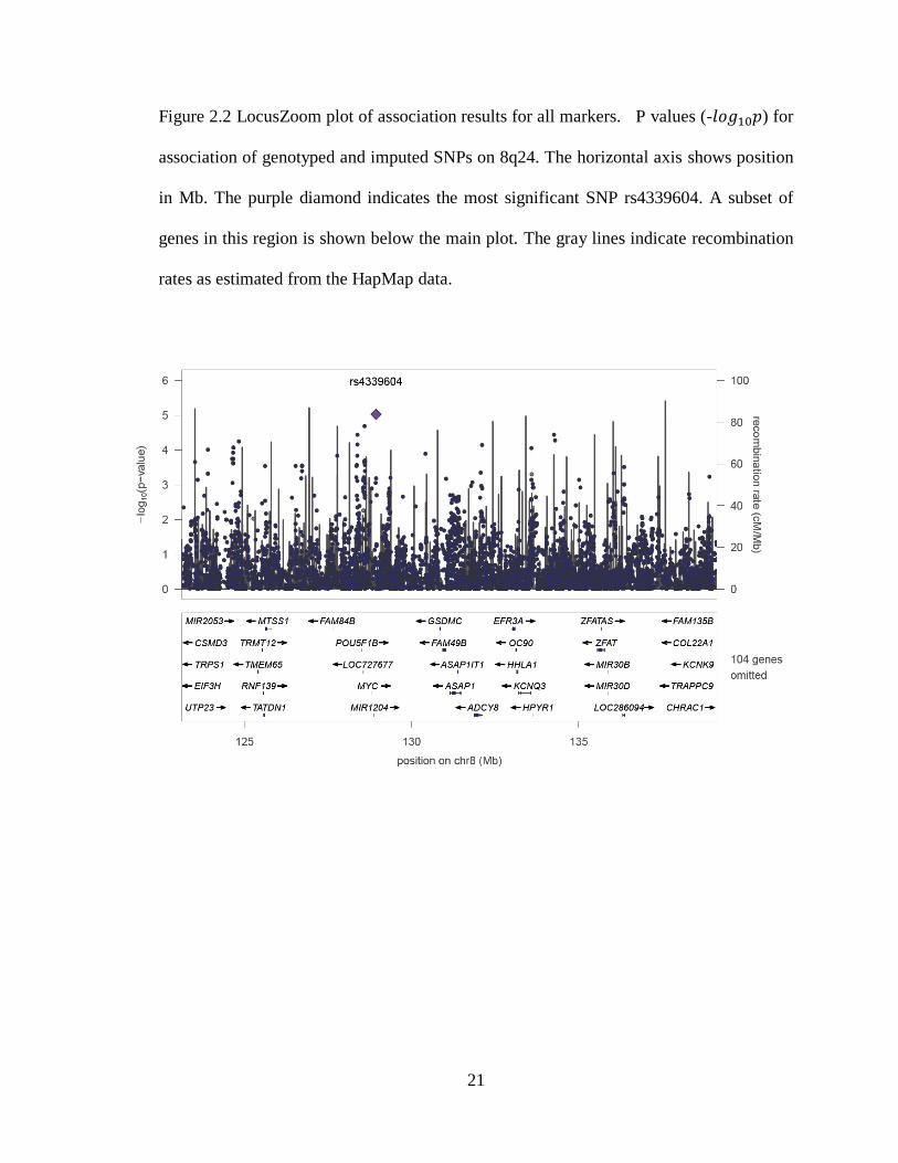
We tested the imputed genotypes of 15,552 SNPs for association with BP using LAMP.
Our results showed 11 SNPS with p-values <10-4
level, with the most significant being
rs4339604 (p = 9.4×10⁻⁶
, MAF = 0.057, physical position = 128.93 Mb), followed by
rs7824868 (p = 2.1×10⁻⁵
, MAF = 0.11, physical position = 128.59 Mb) (Figure 2.2).
Note that the most significant result near 128 Mb is located in a gene desert.
2.4 Discussion
We analyzed a sample of 3,512 individuals in 737 families and tested 2,756 genotyped
SNPs spanning ~16 Mb across the previously identified linkage peak in 8q24 region
(McQueen et al. 2005). Furthermore, we imputed and tested all common HapMap SNPs
in this region. Among the genotyped markers, the most significantly associated SNPs are
located close to 133 Mb near KCNQ3, which is consistent with the linkage peak
identified by genome-wide linkage analysis. Our result provided further suggestive
evidence that supported genetic variants in ST3GAL1 or ADCY8 may be associated with
BP (Table 2.1) (Zandi et al. 2007; Zandi et al. 2008). This association signal is more
significant than our previous results (Zandi et al. 2008), it is difficult to assess
experiment-wide statistical significance. Correcting for the number of sequenced markers

15
tested results in a corrected p = 0.13, for the most significant finding (4.8 x 10⁻⁵
).
However, Bonferroni correction assumes independent tests and the SNPs in this region
are highly correlated. Moreover, permutation analysis cannot be applied to assess
significance because of the family structure in our dataset. Hence it is not clear how to
assign experiment-wide significance levels. Including imputed SNPs added additional
signals with suggestive evidence for association, although no SNPs were significant after
stringent (Bonferroni) correction for multiple testing.
All genes implicated by our analysis have previously been implicated as candidates for
bipolar and other psychiatric disorders. KCNQ3 has been shown to be expressed highly
specific to brain and co-expressed with KCNQ2 in most brain regions (Schroeder et al.
1998). KCNQ2 has been implicated to be associated with BP through phosphatidyl-
inositol phosphate pathway (Carter 2007) and both KCNQ2 and KCNQ3 are key
components to form a voltage-gated potassium channel that is important in the regulation
of neuronal excitability (Schroeder et al. 1998). Although no peer-reviewed evidence has
been forthcoming on KCNQ3 as a susceptibility gene for BP disorder, a recent published
US patent proposed using a single nucleotide mutation in KCNQ3 gene to assess the
presence of or predisposition to schizophrenia, BP or a related mental disorder in a
subject (Chumakov et al. 2006). Furthermore our findings have an intriguing connection
to replicated GWAS results. ANK3 anchors voltage-gated sodium channels, and both
ANK3 and subunits of the calcium channel are down-regulated in response to lithium
treatment in mice (McQuillin et al. 2007). Hence, both the results from ANK3 and that of
KCNQ3 support the involvement of an ion channelopathy in bipolar disorder (Gargus

16
2006), which was also supported by pathway-based analyses on GWAS data in BP
(Askland K et al. 2009).
The product of ADCY8 catalyzes the formation of cyclic AMP from ATP, where cyclic
AMP may be involved in BP pathogenesis as a target for lithium and other mood
stabilizing agents (Perez et al. 2000; Stewart et al. 2001). Malsen et al. showed that
ADCY8 was differentially expressed in specific brain region as a function of avoidance
behavior in mice. The author further explored the human homologous 8q24 region using
a candidate gene approach to test association with BP with genotypes from a GWAS and
reported nominally significant associations with ADCY8 (p = 0.0055) and KCNQ3 (p =
0.0029) (De Mooij-van Malsen et al. 2009).The product of ST3GAL1 gene is a type II
membrane protein that catalyzes the transfer of sialic acid from CMP-sialic acid to
galactose-containing substrates. A recent family-based association of candidate genes
reported evidence of association of ST3GAL1 to BP (empirical p value < 0.005) (Ferreira
et al. 2008).
As none of the signals we observed can sufficiently explain the linkage signal in 8q24, it
is likely that additional BP-variants exist in this region. However, as testing 15,552
additional imputed SNPs did not generate additional interesting signals, our panel of
2,756 SNPs likely captured most of the common haplotype variation in the 8q24 region.
Therefore, typing additional common variants in this region would not result in new
findings. Our results clearly show that the common variants in the 8q24 region do not
explain the previously observed linkage peak (Dick et al. 2003). This result may be

17
explained by one of two reasons: (1) The linkage peak may be a false positive, and the
replications of the linkage peak are the result of publication bias. (2) The causal genetic
variants in this region may be individually rare SNPs or copy number variants, which
association tests of common SNP markers have low power to detect. To assess the
contribution of rare variants in 8q24, it will be necessary to sequence a set of candidate
genes, or the entire 8q24 region in a sample of BP cases. Our results pinpoint to at least
two potential starting points.
In summary, we identified three biologically feasible signals for association with BP but
more research is required to understand the contribution of genes in the 8q24 region to
bipolar disorder.

18
Table 2.1 Top 10 results of single marker association tests. Results are for genotyped
markers. I performed the tests under a multiplicative model with a disease prevalence of
1% using LAMP (Gargus 2006).
Marker Position(Mb) MAF Gene Location LOD P value
rs2673582 133.59 0.425 KCNQ3 27Kb upstream 3.59 4.80E-05
rs4871780 128.36 0.421 3.20 1.20E-04
rs3750889 132.07 0.406 ADCY8 intron 2.63 5.00E-04
rs1023096 132.10 0.419 ADCY8 intron 2.49 7.00E-04
rs6986303 134.55 0.289 ST3GAL1 intron 2.32 1.10E-03
rs6984550 133.63 0.200 KCNQ3 64Kb upstream 2.27 1.20E-03
rs10095649 135.23 0.133 1.96 0.0026
rs4523235 132.31 0.303 1.95 0.0027
rs10094837 135.27 0.138 1.93 0.0028
rs17602731 133.59 0.314 KCNQ3 32Kb upstream 1.89 0.0032
MAF: minor allele frequency

19
Figure 2.1 LocusZoom plot of association results for genotyped markers. The top figure
shows p values (- ) from association test for each genotyped SNPs versus position
(Mb) across linkage peak on 8q24 (McQueen et al. 2005). The bottom figure magnifies
one Mb surrounding the most significant maker rs2673582 (purple diamond). Below each
plot, a subset of genes in this region is shown. Light gray lines display recombination
rates as estimated from the HapMap data. The colors of the circles indicate the strength of
linkage disequilibrium (LD) with rs2673582.

20
21
Figure 2.2 LocusZoom plot of association results for all markers. P values (- ) for
association of genotyped and imputed SNPs on 8q24. The horizontal axis shows position
in Mb. The purple diamond indicates the most significant SNP rs4339604. A subset of
genes in this region is shown below the main plot. The gray lines indicate recombination
rates as estimated from the HapMap data.

22
Chapter 3 Genotype imputation reference panel selection using
maximal phylogenetic diversity
3.1 Introduction
Genotype imputation is an essential component of modern genetic association studies.
This technique enables direct testing of untyped markers for associations with phenotypes
of interest, thereby increasing the power to identify causal variants in association studies
(Li et al. 2009). Imputation is especially useful in meta-analyses that combine data from
genome-wide association studies (GWAS) performed using different genotyping
platforms (Zeggini et al. 2008; Scott et al. 2009). Moreover, genotype imputation
performed using study-specific sequenced samples enables analysis of rare variants
in large GWAS genotyped datasets (Zawistowski et al. 2010).
Imputation methods typically use a reference panel of densely genotyped haplotypes to
predict the missing genotypes in a less densely genotyped study sample. The choice of
the reference panel then influences the imputation accuracy obtained in the study sample.
It has been observed that in general, imputation accuracy is higher when the reference
panel and the study sample derive from the same or similar populations than when they
are from substantially different groups (Huang et al. 2009; Huang et al. 2011). However,
high-diversity reference panels also contribute to increased imputation accuracy. Huang
et al. (2009) found that increasing reference panel diversity by incorporating a mixture of
different HapMap populations could increase imputation accuracy in comparison with the

23
use of only a single HapMap population. Similarly, in imputing a study sample from a
British birth cohort, Jostins et al. (2011) found that adding to the reference panel a
proportion of HapMap samples from other populations (e.g., taking 17% of the reference
panel from Toscani or 22% from Chinese and Japanese) yielded a higher imputation
accuracy than using Northern European samples alone.
Most studies performed to date have selected reference panels from external databases
such as the International HapMap Project (The International HapMap Consortium 2005;
Frazer et al. 2007) and the 1000 Genomes Project (The 1000 Genomes Project
Consortium 2010). Dramatic reductions in sequencing cost now enable an alternative
strategy: to select an internal reference panel for genotype imputation, that is, to
sequence a subset of the study sample itself and then to use the sequenced subset as a
reference panel for imputing the rest of the study sample. Using reference sequences
derived from the study sample can prevent a mismatch in ancestral background between
the study population and the reference population. It also enables novel variants
distinctive to the study sample to be imputed. Employing sequences from a candidate
gene and the 1000 Genomes Project, Fridley et al. (2010) demonstrated the feasibility of
imputing genetic variants based on a sequenced proportion of a study sample, and they
suggested sequencing “the largest and most diverse” subset. In a theoretical study, Jewett
et al. (2012) found that including sequenced haplotypes from the study population in the
reference panel improved imputation accuracy, even if the external panel was taken from
a closely related population. Here, we develop criteria for the selection of an internal
reference panel for genotype imputation. Our goal is to find a sensible approach for

24
choosing an internal reference panel from the study sample, with the aim of 1)
maximizing the number of polymorphic sites in the imputed dataset and 2) achieving the
maximal imputation accuracy.
The identification of maximally diverse subsets of a larger set of individuals has been a
goal in other areas of genetics, such as in choosing diverse sets of plant accessions for
inclusion in core collections targeted for agronomic development or experimental use
(Brown 1989; McKhann et al. 2004; Reeves et al. 2012) and in choosing diverse species
sets for biodiversity conservation (Faith 1992; Steel 2005) and genome sequencing (Pardi
and Goldman 2005). In selecting a set of imputation templates, we borrow the concept of
“phylogenetic diversity” which, for a given subset of a larger set of taxa, measures the
fraction of the total branch length of an evolutionary tree of the larger set that is included
in the restriction of the tree to the taxon subset (Faith 1992; Nee and May 1997; Steel
2005). Conditional on a tree of n taxa, Pardi and Goldman (2005) and Steel (2005)
proved that among all possible subsets of size m ≤ n taxa from the larger set, the globally
maximal phylogenetic diversity can be obtained by a greedy algorithm. This greedy
algorithm provides a computationally efficient solution to a form of combinatorial
optimization problem that can usually only be solved via exhaustive analysis of all
possible subsets. Further, if it becomes possible for investigators to increase the number
of sequenced samples, for example, by an increase in budget, then the greedy algorithm
guarantees that all of the previously selected individuals will be included in the larger
optimal subset.

25
We propose the use of the most diverse reference panel for genotype imputation, adapting
the greedy algorithm for maximizing phylogenetic diversity in our selection of an internal
reference panel. We assume phased diploid individual genotypes are available, as phasing
is not our focus. We approximate the ancestral relationships of haplotypes by
constructing a neighbor-joining phylogenetic tree (Saitou and Nei 1987) using the
pairwise Hamming distance matrix between the haplotypes in a study sample (Figure
3.1). We next apply the greedy algorithm of Pardi and Goldman (2005) and Steel (2005)
to identify the subset at a given size with the maximal “phylogenetic diversity”
conditional on the tree. Similar to a method of template selection by Pasaniuc et al.
(2010), our approach is tree-based, but we aim to choose a maximally diverse subset,
whereas Pasaniuc et al. (2010) select a subset from an external dataset based on similarity
between haplotypes in the external dataset and each individual haplotype in the study
sample. The haplotypes chosen by our method are spread across the tree and tend to have
long external branch lengths (Figure 3.1, bold lines), as our method prioritizes individual
sequences that are more differentiated. We expect that in comparison with a random
subset, the subset that is most phylogenetically diverse at the genotyped markers also
carries a larger number of polymorphic sites that can be identified by sequencing, and
that are then available for imputation into the remaining sample when this sequenced
subset is used as a reference panel. Thus, this strategy enables more variants to be
imputed in the study sample than with the use of a randomly selected reference panel.
Kang and Marjoram (2012) recently proposed a similar tree-based sample-selection
strategy for next-generation sequencing. Their method selects a subset based on the

26
unweighted pair group method with arithmetic mean (UPGMA) (Sokal and Michener
1958), which is designed for ultrametric data in which each haplotype has the same
distance to the root of the constructed tree. The subtree identified by the method of Kang
and Marjoram (2012) also requires the ultrametric assumption in order to have a maximal
tree length. In contrast, the neighbor-joining method we use does not require data to be
ultrametric.
To evaluate the performance of our "most diverse reference" panel in genotype
imputation, we simulate sequences and create study samples similar to those observed in
GWAS by masking the genotypes for a number of single nucleotide polymorphisms
(SNPs). We then impute the masked genotypes in the study sample by using either the
most diverse reference panel or by using randomly selected reference panels. We also
apply the “most diverse” method to sequences of European ancestry from the 1000
Genomes Project. The results from both the simulated sequences and the 1000 Genomes
sequences show that the most diverse reference panel consistently provides higher
imputation accuracy, independent of imputation lengths, reference panel sizes, and
marker densities in the study sample. We thus provide a cost-effective strategy for
designing sequencing studies for samples with existing genome-wide genotype data. As
of 2013, thousands of GWAS have been performed, with over one million genotyped
individuals (http://www.genome.gov/gwastudies/). Effective use of the genotype data
will make it possible to carry out large-scale sequencing studies on these individuals in
silico with a limited budget.

27
3.2 Materials and methods
3.2.1 Phylogenetic diversity
We use notation similar to that of Steel (2005). Assume a study sample T of n haploid
individuals, each containing q polymorphic sites that are genotyped for k < q variable
sites (referred to as markers) in a region of interest. We consider haploid data (phased
diploid individuals for humans), as we do not focus on phasing. Based on the genotypes
at those k markers, we aim to identify a subset of size m ≤ n to be sequenced.
Sequencing reveals r ≤ q - k additional variable sites in the m individuals. S is then used
as a reference panel to impute the genotypes of these r sites in the remaining n - m
individuals in the study sample T.
To identify the optimal selection of S, let XT be an unrooted tree constructed using all
haplotypes in T on the basis of the k markers. Let λT be the sum of the branch lengths for
all edges of XT. We denote by XS the induced tree obtained by restricting XT to only the
haplotypes in S and by λS the sum of the branch lengths of XS. For m ≥ 2, we define the
size-m subset of T with maximal phylogenetic diversity as pdm:
{ | | }.
3.2.2 Identifying the subset with maximal diversity
To find pdm, we first generate an unrooted tree from the study sample T. Based on the
genotypes of the k markers, we compute the Hamming distances between individual

28
haplotypes and construct a pairwise distance matrix for T. Based on this distance matrix,
we construct a tree using the neighbor-joining method, which recursively agglomerates
pairs of nodes until all nodes have been incorporated into the tree (Saitou and Nei 1987).
On this tree, we apply a greedy algorithm to identify the subset S with size m that has the
maximal phylogenetic diversity. Briefly, we first select the pair of haplotypes with the
greatest distance on the tree and add the pair to S. We then sequentially incorporate as the
next haplotype in S the haplotype that adds the maximal length to the chosen tree at that
step, repeating the process until S reaches size m. Pardi and Goldman (2005) and Steel
(2005) proved that conditional on the tree, the subset chosen according to this greedy
algorithm has the maximal phylogenetic diversity.
3.2.3 Simulations
We analyze simulated datasets to evaluate the performance of the “most diverse reference
panel” in genotype imputation. We independently generate 50 datasets of 2000
haplotypes each with the program ms, a coalescent-based sequence sampling program,
under the neutral Wright-Fisher model (Hudson 2002). We assume a basic population-
genetic model with constant effective population size Ne = 10,000, a mutation rate µ =
1.0-8
per site per generation, and a recombination rate ρ = 1.0-8
per site per generation.
We remove singletons from the simulated sequences to create the "true" imputable
sequence data. All simulated sites are assumed to have at most two alleles. Emulating the
density of current genotype arrays, we select the marker panel of the study sample (the
"genotype data") by randomly choosing 300 markers per Mb that have MAF > 0.1 in the
sequence data. We mask the genotypes for the remaining sites, which become the set of
sites that will be imputed. We simulate haplotypes of length 1 Mb, imputing the middle

29
100 kb while keeping the genotypes for the marker panel in both 450-kb flanking regions
to improve imputation accuracy and to avoid edge effects (Li et al. 2010). Based on these
simulated marker genotype datasets, we apply our algorithm on the marker panel to
obtain the most diverse reference panels of 200 haplotypes. To evaluate the performance
of the most diverse reference panel, for each of the 50 simulated datasets, we generate
1000 random reference panels, by sampling without replacement 200 haplotypes each
from the sequence data for comparison. We ignore the pairing status of two haplotypes in
a diploid individual when selecting the most diverse panel. In practice we can not only
sequence one chromosome in a diploid individual. To incorporate this more realistic case,
we consider the pairing status in diploid case and form the “diverse diploid panel”. If we
plan to sequence 100 diploid individuals out of 1000 diploid individuals, we form the
diverse diploid panel by continuing to incorporate diploid individuals who carry one or
two haplotypes into the panel from the top diversity list until we reach 100 diploid
individuals. In each reference panel, we unmask all imputable sites and use the resulting
sequences as references for genotype imputations. For each dataset, we perform one
imputation with the most diverse reference panel, one imputation with the diverse diploid
reference panel, and one imputation with each of the 1000 randomly selected reference
panels.
To evaluate the impact of our parameter choices, we modify this basic design by
changing the length of the imputation target, the reference panel size, and the number of
genotyped SNPs in a study sample while maintaining the other parameters fixed as
described above. We consider imputation target lengths of 100 kb, 500 kb, 1 Mb, and 2

30
Mb, each time adding 450 kb flanking regions. We select reference panel sizes of 100,
200, 300, 400, and 500 haplotypes among a total of 2000 haplotypes. We also vary the
number of genotyped markers from 300 to 1000 in a 1 Mb region in a study sample. For
each scenario, we simulate 50 datasets of 2000 haplotypes each. For each dataset, we
perform one imputation with the most diverse reference panel and 50 imputations with
randomly selected reference panels.
Based on previous comparisons among imputation methods (Hao et al. 2009; Nothnagel
et al. 2009; Pei et al. 2010), we employ minimac (Howie et al. 2012) as one of the best-
performing methods. This method is an extension of MaCH (Li et al. 2010) for phased
diploid data. To assess imputation accuracy on heterozygous genotypes, we then create
n/2 diploid individuals by randomly combining pairs of haplotypes from the entire study
sample. After imputation, we evaluate the predicted imputation accuracy by examining
for each selected reference panel the mean of the estimated correlation coefficient
across all markers. To evaluate the imputation accuracy of the r imputed sites for the n/2
diploid individuals in the imputed datasets, we compute two measures for the discordance
rate between the imputed genotypes and the simulated genotypes at variant site
in target individual . We let and equal to 0, 1 and 2, based on their numbers of
copies of one specific allele. First we calculate discordance rate across all sites:
∑ ∑ | |
.
As this error function is strongly affected by the minor allele frequencies of the variant

31
sites examined (Huang et al. 2009), we also calculate imputation errors across all
heterozygous genotypes ( ):
∑ ∑ | |
∑ ∑
.
3.2.4 The 1000 Genomes Project data
We apply our method to sequence data from the 1000 Genomes Project. We consider the
phased data of 381 diploid individuals (762 haplotypes) with EUR (European) ancestry,
including 87 CEU (Utah residents with Northern and Western European ancestry), 93
FIN (Finnish from Finland), 89 GBR (British from England and Scotland), 14 IBS
(Iberian populations in Spain), and 98 TSI (Toscani in Italy)
(http://www.sph.umich.edu/csg/abecasis/MACH/download/1000G-PhaseI-Interim.html,
the 1000G Interim Phase I Haplotypes 11/23/2010 release). We remove singletons from
the sample, selecting eight 100-kb regions that are approximately evenly distributed
across chromosome 20. We create study samples using a similar procedure as the
simulation above: for each region, we add a 450-kb flanking region on each side,
randomly choose ~300 genotyped SNPs per Mb among markers with MAF ≥ 0.1, and
mask the genotypes of all other sites. In each region, we select the most diverse 160
haplotypes from the set of 762 total haplotypes as the diverse reference panel. For
comparison, we sample without replacement 1000 random reference panels of 160
haplotypes each.

32
We next consider the entire chromosome 20 and create a study sample using the same
procedure as in the 100 kb regions. We select the most diverse reference panel using our
method and 50 reference panels randomly without replacement. Using the selected
reference panels, we impute all the masked genotypes and compute the discordance rate
for each imputation.
3.3 Results
3.3.1 Number of imputed sites
Polymorphic sites in reference panels: Only sites that are polymorphic in the reference
panel can be imputed into the remaining study sample. Hence, we first evaluate the
number of polymorphic sites in the reference panels selected. For each of the 50
simulated datasets, we choose one random reference panel and compare it to the most
diverse reference panel. We find that for a total of 12,957 masked sites that are
polymorphic in the study samples across the 50 datasets, 9,642 of sites (74.41%) are
polymorphic in both types of reference panels. Among the remaining sites, 1,492 sites
(11.52%) are polymorphic only in the most diverse reference panels, whereas 760 sites
(5.87%) are polymorphic only in the randomly selected reference panels. Thus, on
average, 5.65% more sites are polymorphic in the most diverse reference panels than in
the randomly selected reference panels.
Polymorphic sites in imputed datasets: To ensure that the higher number of polymorphic
sites in the most diverse reference panels also leads to a higher number of imputed
polymorphic variants, we count the number of imputed sites that are polymorphic in
datasets imputed with reference panels generated under three different selection

33
strategies: (1) sampled at random, (2) selecting the 200 most diverse haplotypes and (3)
selecting the diverse considering the haplotype pairing status (diverse diploid reference
panel). As it is not currently practical to sequence only one chromosome in a diploid
organism, strategy (3) represents a scenario in which the individuals that carry the most
diverse haplotypes are identified and both of their chromosomes are sequenced. Across
the 50 datasets, the mean number of haplotypes that one diverse diploid panel of 200
incorporates from the top diversity list is 106, ranging from 102 to 112. Assuming Hardy-
Weinberg equilibrium, this second chromosome is sampled randomly from the
population.
From the total of 12,957 imputed sites across the 50 datasets, 10,952 are polymorphic in
datasets imputed with the most diverse reference panels (84.53%), 10,574 are
polymorphic for the diverse diploid reference panels (81.61%), and 10,151 are
polymorphic for randomly selected reference panels (78.34%). Figure 3.2 shows
percentages of polymorphic sites in datasets imputed with the three reference types across
the 50 datasets. In each of the 50 datasets, imputation with the most diverse reference
panel captures more polymorphic sites than imputation with the random reference panel.
The improvement by using the most diverse panel is greater when the randomly selected
panel captures only a low percentage of polymorphic sites (e.g., replicates 46 to 50).
Imputations with the diverse diploid panels result in higher percentages of polymorphic
sites than the random panels in 42 of the 50 datasets (84%) and in a higher percentage of
polymorphic sites than the most diverse panel in 4 of the 50 datasets (8%). Only in four
datasets does the random reference panel perform substantially better than the diverse

34
diploid reference panel (replicate 1, 2, 3, and 6) and in all these cases, the random panel
captures a high (> 83%) percentage of polymorphic sites.
3.3.2 Imputation accuracy
As a measurement of imputation accuracy, we evaluate the discordance rate between the
simulated genotypes and the imputed genotypes for the 50 simulated datasets. For each
dataset, we compare the accuracy of the imputation using the most diverse reference
panel to the empirical distribution of imputation accuracies from 1,000 random reference
panels.
Estimated imputation quality: A predictor for the accuracy of an imputed site generated
by minimac is the , a quantity calculated by comparing the variance of observed
genotype scores with the variance of expected genotype scores to estimate the squared
correlation at a marker between the true allele counts and the estimated allele counts (Li
et al. 2010). To compare this predicted imputation accuracy between the different choices
of reference panels we compute the average across the 12,957 total imputed sites
across the 50 datasets. For imputations with the most diverse reference panels and the
diverse diploid reference panels, we generate one value of for each site; to evaluate
imputations with the 1000 randomly selected reference panels for each dataset, we
compute the mean for each site across 1000 imputations, and we then calculate the
average across all imputed sites. Sites imputed with the most diverse reference panels
have the highest mean 2 (0.784), followed by sites imputed with the diverse diploid
reference panels (0.758). Sites imputed with randomly selected reference panels have the
lowest mean (0.723). As removing variant sites with filters most poorly

35
imputed sites (Li et al. 2009), we also compare the number of sites that pass this
imputation quality threshold. Across the 50 datasets, we observe that a higher percentage
of sites imputed with the most diverse reference panels pass the threshold (83.17%)
compared to sites imputed with the diverse diploid reference panels (80.53%) and sites
imputed with the randomly selected panels (77.48%). For a higher threshold of 0.8
applied by typical association studies, 76.63% of sites pass the threshold for imputations
with the most diverse reference panels, 74.76% for the diverse diploid reference panels,
and 59.65% for the randomly selected reference panels.
Discordance rates: For each simulated dataset, we separately calculate discordance rates
for all sites imputed with the most diverse reference panel, sites imputed with the diverse
diploid reference panel, and the mean values for sites imputed with random reference
panels taken across all 1000 random panels. Using the most diverse reference panel
results in the lowest mean discordance rate across the 50 replicates (0.0019), followed by
imputation with the diverse diploid reference panel (0.0022). Both quantities are lower
than the mean discordance rates of imputation with the random reference panels (0.0031)
(Figure 3.3). Ranking the discordance rate of selected reference panels together with the
discordance rates of 1000 random panels from the lowest to the highest value, the most
diverse reference panel is a clear outlier for 24 of the 50 datasets (48%), having a lower
discordance rate than imputations with all 1000 randomly selected reference panels (rank
1). Across all 50 datasets, the mean rank of the most diverse reference panel is 13.5,
ranging from 1 to 135 among 1001 panels. Across the same 50 datasets, the mean rank of
the diverse diploid reference panel is 111.9, ranging from 1 to 906 among 1001 panels.

36
To generate a more meaningful discordance measure for low-frequency variants, we also
compare the imputed genotypes and the simulated true genotypes across sites for which
the true genotypes are heterozygotes. While the heterozygote discordance rate is higher
than the overall discordance rate, the mean heterozygote discordance across the 50
replicates is again the lowest for sites imputed with the most diverse reference panels
(0.0097), followed by the diverse diploid reference panels (0.0121) and the random
reference panels (0.0165). Comparing across frequency bins, we observe that for all
reference selection strategies, the heterozygote discordance rate decreases with increasing
allele frequency. The mean heterozygote discordance rate across the 50 replicates for
low-frequency variant sites (0 < MAF < 0.1) is considerably higher than the overall mean
discordance rate for all heterozygote sites across the 50 replicates (0.0258 for the most
diverse reference panels, 0.0329 for the diverse diploid reference panels, and 0.0415 for
the random reference panels). In all frequency bins, considering heterozygote discordance
rates, imputations with the most diverse reference panels generate the lowest discordance
rates and imputations with the randomly selected reference panels generate the highest
discordance rates, while imputations with the diverse diploid reference panels generate
intermediate discordance rates (Figure 3.3). Combining the heterozygote discordance
rate of the most diverse reference panel with the heterozygote discordance rates of 1000
random panels for each of the 50 simulated datasets and ranking from the lowest to the
highest heterozygote discordance rate, the mean rank of the most diverse panel across all
50 datasets is 17.5 when comparing all heterozygote sites, 27.3 for sites with 0 < MAF <
0.1, 115.7 for sites with 0.1 ≤ MAF < 0.2, and 68.5 for sites with 0.2 ≤ MAF ≤ 0.5 out of

37
1001 panels ranked. When comparing the diverse diploid reference panel to random
panels, the mean rank across all 50 datasets is 147.9 for all heterozygote sites, 188 for
sites with 0 < MAF < 0.1, 163.9 for sites with 0.1 ≤ MAF < 0.2, and 145.9 for sites with
0.2 ≤ MAF ≤ 0.5.
3.3.3 Imputation accuracy under different simulation settings
To assess the robustness of our results, we evaluate the performance of the most diverse
reference panel under different simulation settings, considering different target sequence
lengths, different reference panel sizes, and different marker densities in the study
sample. We first investigate whether the lengths of the target regions affect the
performance of the most diverse reference panels in imputations. We impute regions with
lengths of 100 kb, 500 kb, 1 Mb and 2 Mb, using both the most diverse reference panel
and 50 random reference panels, each of which is compared to the true underlying
genotypes; the average of the 50 discordance rates is then compared with the discordance
rate for the most diverse reference panel. As shown in Figure 3.4a, across the four
different lengths, we observe little effect of the imputation length on the discordance rate.
The mean discordance rate across the 50 replicates for each group ranges from 0.0028 (2
Mb) to 0.0037 (500 kb) for the most diverse reference panel and from 0.0052 (2 Mb ) to
0.0058 (100 kb) for the random reference panels. For all sequence lengths considered, the
most diverse reference panels provide lower discordance rates than the randomly selected
reference panels.
Second, we evaluate how the reference panel sizes affect the performance of the most
diverse reference panel by comparing the genotype discordance rates for reference panels

38
of size 100, 200, 300, 400, and 500 haplotypes. For both reference panels, the mean
discordance rate across the 50 replicates decreases with larger reference panel sizes, from
0.008 to 0.0006 for the most diverse panel and from 0.009 to 0.0015 for the random
reference panels. Especially for a reference panel of size 100 individuals, the discordance
rate is considerably higher than for larger panel sizes. Across all reference panel sizes,
imputations with the most diverse reference panels consistently provide lower
discordance rates than do imputations with the randomly selected reference panels
(Figure 3.4b).
Third, we examine how the number of markers genotyped initially in the study sample
affects the performance of the most diverse reference panel by varying the density of
markers in the study sample, considering 200, 300, 400, 500, 600, and 1000 markers per
1 Mb region. For both types of reference panels, the mean discordance rate across the 50
replicates decreases with a higher density of markers in the study samples, from 0.0055 to
0.0015 for the most diverse panel and from 0.0072 to 0.0023 for the random reference
panels. Across all marker densities in the study sample, the most diverse reference panels
consistently provide lower discordance rates than the randomly selected reference panels
(Figure 3.4c). We also observe that the improvement in discordance rates for the most
diverse reference panel over the randomly selected panels slightly decreases with more
markers genotyped in the study sample.

39
3.3.4 Imputation accuracy on data from the 1000 Genomes Project
We apply our method to real sequence data of 381 phased individuals with EUR ancestry
from the 1000 Genomes Project. Considering eight 100-kb regions across chromosome
20, we impute 3,215 sites after removing singletons. Sites imputed with the most diverse
reference panels have a mean 2 of 0.749 across sites; sites imputed with the 1000
randomly selected reference panels have a mean 2 of 0.741. Slightly more sites pass the
imputation quality threshold of 2 ≥ 0.3 for the most diverse reference panels (85.75%)
than for the randomly selected reference panels (84.23%). When applying a higher
imputation threshold of 2 ≥ 0.8, a similar percentage of sites pass the threshold for the
most diverse reference panels (62.74%) and the randomly selected reference panels
(62.89%).
Considering all imputed sites for the eight 100-kb regions, the most diverse reference
panels result in a lower mean discordance rate across the eight regions (0.0067) than the
randomly selected reference panels (0.0077). When comparing imputed sites that are
heterozygotes in real sequenced datasets, sites imputed with the most diverse reference
panels have a lower mean discordance rate across the eight regions (0.0228) than sites
imputed with the randomly selected reference panels (0.0262). The lower discordance
rates from the most diverse reference panels are observed across all frequency bins for
heterozygote sites: For sites with 0 < MAF < 0.1, the mean discordance rate across the
eight regions is 0.074 using the most diverse reference panels versus 0.0895 using
random reference panels, for sites with 0.1 ≤ MAF < 0.2, the mean discordance rate
across the eight regions is 0.0177 versus 0.0193, and for sites with 0.2 ≤ MAF ≤ 0.5, the

40
mean discordance rate across the eight regions is 0.0080 versus 0.0099 (Figure 3.5).
However, we also notice that the performance of the most diverse reference panel varies
widely among the eight regions. When ranking the discordance rate of the imputation by
the most diverse reference panel with the discordance rates of the 1000 imputations by
randomly selected reference panels from the lowest to the highest value for each of the
eight regions, the most diverse reference panel has an average rank of 116.1 across the
eight regions, ranging from 3 to 496 out of 1001 panels ranked. For heterozygote sites,
the most diverse reference panel has an average rank of 156.7, ranging from 1 to 508; for
heterozygotes in different MAF bins, the most diverse reference panel has an average
rank of 242.7 for sites with 0 < MAF < 0.1, an average rank of 311.0 for sites with 0.1 ≤
MAF < 0.2, and an average rank of 129.4 for sites with 0.2 ≤ MAF ≤ 0.5 out of 1001
panels ranked.
For the whole chromosome 20 data, the sequence dataset contains 259,618 sites after
removing singletons. We select 18,000 sites with MAF ≥ 0.1 as “genotyped” markers and
mask the genotypes for the remaining 241,618 sites to create a study sample. Based on
the genotyped markers, we select the most diverse reference panel to impute the
genotypes of the masked sites. For comparison, we sample 50 reference panels at
random. We first compare the number of masked sites that are polymorphic in the
selected reference panels. In the most diverse reference panel, 211,480 masked sites are
polymorphic (87.53%), compared to an average of 210,137 across the 50 random
reference panels (86.97%). After imputation, we observe that the imputation with the
most diverse reference panel has 201,831 sites with 2 ≥ 0.3 (83.53%), whereas 200,609

41
sites have mean 2 ≥ 0.3 with a randomly selected reference panel (83.03%). For the
higher imputation quality threshold of 2 ≥ 0.8, 142,996 sites pass the threshold for the
imputation with the most diverse reference panel (59.18%), whereas averaging 142,281
sites across imputations with the 50 randomly selected reference panels pass the threshold
(58.89%). Moreover, sites are imputed slightly more accurately with the most diverse
reference panel than with random reference panels (Table 3.1). The discordance rate of
the most diverse panel is lower than all except 2 of the 50 random panels (rank 3). To
evaluate the imputation accuracy in different frequency bins, we again consider
discordance rates of heterozygote genotypes. When ranking the discordance rate of the
imputation by the most diverse reference panel with the discordance rates of the 50
imputations by randomly selected reference panels from the lowest to the highest value,
we observe that the most diverse reference panel has a lower discordance rate than all 50
random panels (rank 1). Examining separate frequency bins, the most diverse reference
panel has rank 4 for sites with 0 < MAF < 0.1, rank 3 for sites with 0.1 ≤ MAF < 0.2, and
rank 14 for sites with 0.2 ≤ MAF ≤ 0.5. Averaging across sites, the numerical
improvement in imputation accuracy by using the most diverse panel is modest, reducing
imputation errors by 1% across all sites and by 2.3% at less common variants with 0 <
MAF < 0.1.
3.4 Discussion
The cost reduction in modern sequencing technology enables investigators to generate a
reference panel for genotype imputation by sequencing a subset of the study sample. We
have proposed a sampling strategy for such an internal reference panel by adapting an
algorithm based on phylogenetic diversity. In simulated sequence data, our method

42
consistently outperforms randomly selected reference panels, in that it provides higher
imputation accuracy and recovers more polymorphic sites from the sample. This
improved performance holds across different imputation lengths, different reference
panel sizes, and different marker densities in the study sample. Upon analyzing real
sequence data with European ancestry from the 1000 Genomes Project, the most diverse
reference panel provides higher imputation accuracy than do randomly selected reference
panels. We observe this improved performance when imputing eight 100-kb regions on
chromosome 20 and when imputing the entire chromosome 20, indicating that our
method can be used to select reference individuals for imputing smaller target regions as
well as for imputing entire genomes. Our method may be particularly advantageous for
imputing less common variants, as we found in our simulations that the most diverse
reference panels have more polymorphic sites than do randomly selected reference
panels. Moreover, the accuracy gain from using the most diverse reference panel instead
of randomly selected reference panels is greater for less common variants (e.g., 0 < MAF
< 0.2) than for more common variants (e.g., MAF ≥ 0.2) (Table 3.1).
Our method is fundamentally different to Pasaniuc (2010). Although both selections are
based on the genotypes of makers that exist in the study sample and reference sequences,
we adapt phylogenetic diversity in our method whereas Pasaniuc and colleague’s method
identifies one different reference panel for each short window (e.g., 15 kb) of the target
region for each study individual based on coalescent theory. In addition, their method
requires having a pool of sequences to select from. This is not the case for our purpose as
we don’t have all the sequences and can only sequence a subset of the study sample.

43
Kang and Marjoram (2012) very recently considered sample selection for next-generation
sequencing using a similar approach based on maximizing the subtree length. Compared
to our NJ method, Kang and Marjoram used the UPGMA tree. In general, the NJ method
is more accurate in computing branch lengths as it considers all taxa on the tree when
estimating branch lengths whereas UPGMA only select the closest neighbors and
compute the arithmetic mean. In addition, Bryant (2005) proved the NJ is statistically
consistent given the distance data whereas UPGMA does not always satisfy the
consistency criteria. Finally, UPGMA requires the ultrametric condition, the final tree is a
clock-like tree and each individual on the tree has the same distance to the root. As a
result, we expect the method based on UPGMA to have more ties that evolve sample
uniformly at random in selecting a subset with maximal tree length than our method as
our NJ tree does not require the ultrametric assumption. Although they have used a
different tree-building algorithm, they examined a similar greedy method, motivated by
coalescent theory instead of from the standpoint of phylogenetic diversity. In simulations
that examined different marker densities, target imputation region lengths, and reference
panel sizes, they found that their algorithm performed well, and we similarly find that our
related method performs well under these scenarios. In addition, the work of Pardi and
Goldman (2005) and Steel (2005) provides further theoretical justification for the basis of
our algorithm, as well as for the method of Kang and Marjoram. Taken together, our
study and that of Kang and Marjoram demonstrate the value of sensible use of
genealogical relationships among samples to improve the experimental design for
sequencing studies. Further, as shown in Pardi and Goldman (2005), our method can

44
incorporate other selection criteria by starting with an initial selection of haplotypes and
then applying the greedy algorithm as an extension.
We expect that the most diverse reference panel algorithm can work effectively either on
a limited region of the genome or on whole chromosomes, provided the phylogenetic tree
based on existing data reasonably captures the ancestral relatedness of the haplotypes in
the study sample. This is only possible if this ancestral relatedness can be described well
as a tree, a condition that depends on the population-genetic history of the sample and the
size of the region of interest. When focusing on a single genomic region, relevant parts of
its ancestral process can be approximated as a tree due to limited recombination events.
This single tree can be estimated by a subset of genotyped markers, and thus, our method
can provide useful information for reference panel selection. On the other hand, many
uncorrelated trees can be formed to represent the ancestral processes of a large region
such as the entire genome. Hence, an approximation with a single tree might not capture
many features of the data. In such a scenario, it is less likely that our method will produce
a better reference panel than a random sample. In a structured population, the underlying
population structure generates a correlation of ancestries across the entire genome. The
resulting clades can be approximated by the tree-building algorithm, and this tree can
help in selecting a more diverse reference panel. It is encouraging that in a sample of five
European subpopulations, the population structure was sufficient for the most diverse
reference panel selected based on the entire chromosome 20 to outperform the randomly
selected reference panels. Hence, relatively subtle population structure, such as that found
in samples from closely related European countries, is sufficient to create similarities in

45
the underlying ancestral processes that can be captured by the tree-building algorithm and
can result in improved reference panel selection. For subpopulations with different
sample sizes, we expect the diverse algorithm only oversample from subpopulations with
many individuals that have dramatic longer external branch lengths that individuals from
other subpopulations on the constructed tree, or undersample in the case of dramatic short
external branch lengths. Otherwise, we expect our algorithm will pick the number of
individuals that are proportional to the size of each subpopulation.
Our method is based on local phylogenetic tree. The topology of the local phylogenetic
tree may change with increasing size of a genome region because of recombination
events. As the performance of our method is based on how well the local phylogenetic
tree approximates the ancestral relatedness of the study individuals, we expect the gain in
imputation accuracy using our method will decrease with increasing length of an
imputation region. As expected, the average improvement in imputation accuracy when
imputing 100-kb regions is considerably higher than the average improvement across the
entire chromosome, reflecting that the ancestry of a 100-kb region is more tree-like than
the ancestry of an entire chromosome. However, the average improvement in imputation
accuracy when imputing 100-kb regions is considerably higher than the average
improvement across the entire chromosome, reflecting that the ancestry of a 100-kb
region is more tree-like than the ancestry of an entire chromosome.
The method of reference panel selection described here can be adapted to address specific
study design goals. Our method can be applied to incorporate other criteria in reference

46
panel selection. For example, we have not specifically incorporated phenotype
information when selecting reference haplotypes, so the selected reference panel is not
guaranteed to include the individuals with traits of interest. To sequence certain
individuals because of their phenotypes or other criteria unrelated to their phylogenetic
placement, we can apply the selection algorithm conditional on including these
individuals in the reference panel. The greedy algorithm still guarantees that the
subsequent extension has optimal phylogenetic diversity, as proved in Pardi and Goldman
(2005). Similarly, our method can be easily extended to form a reference panel by
incorporating sequences partly from the study sample and partly from an external
database such as the HapMap Project or the 1000 Genomes Project. For example, we can
treat sequences from the HapMap Project as an initial set and apply the greedy algorithm
to the study sample as an extension in a similar manner as in analyses treating other
inclusion criteria.
Our method should be applicable to imputation in other species of a genome region in
other species as long as the constructed tree can reasonably represent the ancestral
relatedness among the study individuals. Wang et al. (2012) proposed to use local
phylogenetic tree to provide confidence information in imputing sequences in inbred
mice. The confidence is high for imputing study strains that share one or more genome
intervals with reference sequences, whereas the confidence is low for strains that do not
share genome intervals with reference sequences. The authors also proposed that
sequencing these strains with low confidence imputation quality could provide maximal
improvement in imputation accuracy and new variant identification. The strategy used by

47
Wang et al (2012) may work well as an extension to our study to combine existing
sequence data in imputation. For example, to get the full sequences of a genome region
for a study sample, we can form a reference panel from the 1000 Genomes Project that
share one or more haplotypes with our study sample and impute the sequences of the
these study individuals with high confidence, and apply the our method to the rest of
study individuals or sequencing all the rest of study individuals if budget allows.
In summary, we have demonstrated that an innovative method of choosing an internal
reference panel — the most diverse reference panel — can be a cost-effective approach
for planning sequencing studies with existing genotype array data. The method can
readily incorporate a variety of selection criteria, while still guaranteeing the maximal
phylogenetic diversity for subsequent selections.

48
Table 3.1 Discordance rates for imputations for real sequencing data. Data are from
chromosome 20 of individuals with European ancestry in the 1000 Genomes Project.
Discordance rates are shown as percentages. We split 381 phased diploid individuals into
a target sample of 301 target individuals and a reference panel of 160 haplotypes. Shown
here are results from one imputation with the most diverse reference panel and the mean
and standard deviation of the discordance rates from 50 imputations with randomly
selected reference panels. We ranked discordance rates of the most diverse panel together
with 50 random reference panels from the lowest to the highest value and display the
rank of the most diverse panel.
Reference types Variant groups
All Heterozygotes MAF(0,0.1) MAF[0.1,0.2) MAF[0.2,0.5]
Most diverse 1.02 3.53 10.31 2.77 1.92
Random
mean 1.03 3.57 10.45 2.82 1.93
standard
deviation 0.004 0.019 0.076 0.019 0.014
Rank of the most
diverse 3 1 4 3 14

49
Figure 3.1 Illustration of the selection of the most phylogenetically diverse reference
panel. Shown is the phylogenetic tree constructed from 20 simulated haplotypes as well
as the most diverse subset of five taxa (in bold). The selection algorithm first selects the
most distant pair of taxa and then identifies haplotypes that are most distant conditional
on the haplotypes already selected. To choose the five taxa, the greedy algorithm first
selects pair 1 and 14, and then 12, 19, and 5 sequentially. Notice how the haplotypes
chosen are spread across the tree and possess long branch lengths.

50
Figure 3.2 Percentages of polymorphic sites in imputed datasets. The white bar represents
the accuracy of a random panel, the grey bar represents the accuracy of the diverse
diploid panel, and the black bar represents the accuracy of the most diverse reference
panel. If the performance of the diverse diploid reference panel is lower than the
performance of the random reference panel, this difference is indicated by the part of the
white bar with horizontal stripes. If the accuracy of the diverse diploid panel is higher
than the accuracy of the most diverse panel, this difference is indicated by the part of the
grey bar with vertical stripes. Data are 50 imputed datasets that are sorted in decreasing
order by percentage of polymorphic sites recovered by imputations with random
reference panels.

51
Figure 3.3 Comparison of imputation accuracy. Boxplots of discordance rates between
imputed genotypes and simulated genotypes for imputations with randomly chosen
reference panels, diverse diploid reference panels, and most diverse reference panels. The
mean discordance rate across the 50 replicates for each comparison group is indicated by
a diamond, and the median discordance rate across the 50 replicates for each comparison
group is indicated by a middle line. The horizontal axis labels the comparison on the
basis of all sites (All), all heterozygote sites (Heterozygotes), and heterozygotes in
different MAF groups in the simulated sequence data.

52
Figure 3.4 Imputation accuracy under different scenarios. Boxplots of discordance rates
between imputed genotypes and simulated genotypes for imputations with randomly
chosen reference panels and most diverse reference panels with varying simulation
settings: A. Imputation length; B. Reference panel size; C. Number of genotyped markers
per Mb in the study sample. For each dataset, we examine the mean of 50 random
reference panels and the most diverse reference panel. The mean discordance rate across
the 50 replicate simulated datasets for each comparison group is indicated by a diamond,
and the median discordance rate is indicated by a middle line.

53

54
Figure 3.5 Imputation accuracy on the 1000 Genomes Project data. Boxplots of
discordance rates between imputed genotypes and simulated genotypes for imputations
with randomly chosen reference panels and most diverse reference panels for eight 100-
kb regions on chromosome 20. We analyzed 762 haplotypes of European ancestry from
the 1000 Genomes Project. The horizontal axis represents comparison of all sites (All),
all heterozygote sites (Heterozygotes), and heterozygotes in different MAF groups in the
simulated sequence data. The mean discordance rate across the eight regions for each
comparison group is indicated by a diamond, and the median discordance rate across the
eight regions for each comparison group is indicated by a middle line.

55
Chapter 4 Selecting the most representative sample in genotype
imputation for next-generation sequencing
4.1 Introduction
Genome-wide association studies (GWAS) have successfully identified many of the
common genetic variants for complex diseases. With the dramatic cost reduction in next-
generation sequencing technology, investigators have begun to use sequencing studies to
identify genetic risk variants for complex diseases with a focus on rare variants (Nelson
et al. 2012; Xia et al. 2012). However, sequencing a large study sample is still very
expensive. Thus, we need sampling strategies to select an optimal subset such that we can
identify the maximal number of variable sites in the study sample and achieve the
maximal imputation accuracy when imputing the sequences for the rest of the study
sample using the sequenced individuals as references.
Genotype imputation is a statistical approach that predicts genotypes in a less densely
typed study sample by using information from a more densely genotyped dataset as a
reference panel. The most commonly used reference panels are sequences from the
International HapMap Project (The International HapMap Consortium 2005) and the
1000 Genomes Project (The 1000 Genomes Project Consortium 2010). Investigators have
used these sequences as reference panels to impute the genotypes for untyped HapMap
markers in their GWAS. Here, we aim to identify a subset from a study sample to
sequence and to use the sequenced subset as a reference panel to obtain sequences for the

56
rest of the study sample. Sequencing can identify novel variants that are unique to a study
sample. In addition, compared to imputations with reference sequences from public
databases such as the International HapMap Project, imputations with reference
sequences from the study sample itself avoid the possible ancestral background mismatch
between the reference population and the study population.
We have proposed a sampling strategy for sequencing in Chapter 3, where we propose to
sequence the subset that has maximal subtree length, a panel we term the most diverse
reference panel. We show that the most diverse reference panel incorporates more
polymorphic sties and provides higher imputation accuracy than a randomly selected
reference panel when imputing the sequences of the rest of study sample for individuals
from one population or closely related populations. Kang and Marjoram (2012) proposed
another tree-based method that produced similar results. Both Kang’s method and our
method assume that the number of mutation events is proportional to the genealogical
tree length, thus the subtree with the maximal tree length is expected to carry more
mutant alleles that can be identified by sequencing and consequently to recover more
variants when used as a reference panel. In addition, it assumes that selected haplotypes
are spread across the tree, thus could well represent the unselected haplotypes. However,
this may not be true in some cases, for example, the most diverse subset may oversample
haplotypes in a cluster on the tree that vastly different while fail to sample any haplotypes
in a cluster that are similar with small branch lengths (Bordewich et al. 2008). The most
diverse algorithm also does not count the similarity between the selected subset and

57
unselected subset, thus the haplotypes in the unselected subset may not represented well
by the haplotypes in the selected subset.
Here we propose a subset selection method that considers both the selected subset (R)
and unselected subset (U). We propose the “most representative” subset, defined by the
pair (R, U) such that the summation of minimum distances over all unselected haplotypes
in U to the selected subset R is the smallest among all possible choices of (R, U).
Because of the combinatorial nature of this problem, it is not computationally feasible to
compare all instances for a large sample. By our best knowledge, there is no such existing
approach as the greedy algorithm in Chapter 3 to find such a pair (R,U). Instead, we use a
local search algorithm, known as the hill-climbing search, to search for the most
representative panel. The local search algorithm is not systematic, but it has two key
advantages over an exhaustive search: (1) it uses very little memory – usually constant
amount; and (2) it can often find reasonable solutions in large state spaces for which
systematic algorithms are unsuitable (Russell and Norviq 2009). The goal is to find the
global optimum or a local optimum that is a reasonable approximation of the global
optimum (Selman and Gomes 2006). To increase the chance of reaching the global
optimum and minimize the chance of being stuck in local optimum, we randomly start
multiple times and choose the replicate that has the smallest (R, U) distance as the
starting point for the hill-climbing search (Figure 4.1).
Using simulated sequences as well as sequences from the 1000 Genomes Project, we
compare the characteristics and performance the representative panel to the most diverse

58
panel and randomly selected panels so that we can provide guidelines for investigators to
use when planning sequencing studies with existing genotype data.
4.2 Materials and methods
4.2.1 Define the representative panel
4.2.1.1 Haploid case
Assume a sample of 2n haplotypes, we want to choose 2k haplotypes as a reference panel
(k ≤ n). We represent the selected 2k references in R as I1, I2, …, I2k and represent the
unselected 2n - 2k haplotypes in U as J1, J2, ...., J2n-2k. For each haplotype j є U, we
represent the minimum distance to the haplotypes in R as dj = mini є R {Dji}, where i is the
haplotype in R that is the closest to j and Dji represents the pair-wise Hamming distance
between haplotypes j ϵ U and i ϵ R.
The sum of minimum distance for one realization of R and U, represented by (R, U) is,
( ) ∑ ∑ { }.
Our goal is to find the realization with minimum distance among all possible realizations
of (R, U) with size R2k and U2n-2k, the "minimum of minimums", represented by ( ),
( ) {( )} (∑ { }).

59
4.2.1.2 Diploid case
Assume a sample of 2n haplotypes, which we randomly pair two haplotypes without
replacement and form into n diploid individuals. We want to choose k diploid individuals
out of n phased diploid individuals (k ≤ n). We represent the selected k diploid
individuals in R as (I1a, I1b), (I2a, I2b), ..., (Ika, Ikb) and represent the unselected n - k
individuals in U as (J1a, J1b), (J2a, J2b), …, (J(n-k)a, J(n-k)b), where all the individuals are
phased and they are in arbitrary order.
For each individual j ϵ U, the minimum distance to the selected subset is haplotype i ϵ R,
defined as
( ) ( ) ..
represents the pair-wise Hamming distance between haplotype js and it for s, t ϵ (a,
b).
Our goal is to find the realization with minimum distance out of all the possible
realizations with size Rk and Un-k, represented by ( ),
( ) (∑
)
{∑ ( ( ) ( ) ) }.

60
4.2.2 Hill-climbing search algorithm
Hill-climbing is a greedy local search algorithm that results in a local optimum. To
increase the chance of reaching the global minimum and to speed up the search, we
randomly divide the study sample into R and U with a certain size for 100 times and start
the hill-climbing search with set of (R, U) that has the smallest distances (Figure 4.1).
4.2.2.1 Implementation: haplotype case
1. Randomly select 100 subsets (R0, size 2k haplotypes), calculate the distances of
(R0,U0) for each selection.
2. Select the set of (R0,U0) that has the smallest distance as starting (R, U).
3. Randomly replace one haplotype in R with one haplotype from U, recalculate (R,
U)’, if (R,U)’> (R,U), accept the replacement, otherwise keep the previous subset
selection.
4. Repeat step 3 for 100,000 times, record the final selection of (R, U).
4.2.2.2 Implementation: diploid case
1. Randomly pair two haplotypes into diploid without replacement.
2. Randomly select 100 subsets (R0, size k diploids), calculate the distances of
(R0,U0) for each selection.
3. Select the set of (R0,U0) that has the smallest distance as the starting (R, U).
4. Randomly replace one pair of haplotypes in R with one pair of haplotypes from
U, recalculate (R, U)’. If (R,U)’> (R,U), accept the replacement, otherwise keep
the previous subset selection.
5. Repeat step 4 for 100,000 times, record the final selection of (R, U).

61
4.2.3 Diverse reference panel
The most diverse panel and diverse diploid are the same as described in Chapter 3, which
are obtained from the greedy algorithm.
4.2.4 Imputation accuracy
We employ minimac (Howie et al. 2012) as one of the best-performing methods, which is
an extension of MaCH (Li et al. 2010) for phased diploid data. To evaluate the
imputation accuracy of imputed sites across all individuals in imputed datasets. For each
site j, the concordance rate for the minor allele is
{ ∑ | |
∑
( )}.
and are the simulated genotype and imputed genotype for individual i at site j,
represented by the number of minor alleles in that individual (0, 1 and 2) at that site. n is
the number of diploid individuals in the study sample.
Similarly, the concordance rate for the major allele of site j is
∑ | |
∑ ( )
( )}.
We compute the expected heterozygote concordance rate for site j by
( ) ( ) .
Xj and Yj are the allele concordance rate for the minor allele and the major allele,
respectively.

62
4.2.5 Simulations
We simulate sequence data using the program ms (Hudson 2002) with parameters and
datasets created the same as described in Chapter 3. Briefly we first remove singletons
from the simulated sequences. We create the study samples by randomly choosing ~300
genotyped SNPs per Mb among markers with MAF ≥ 0.1 and mask the genotypes of all
other sites. These masked sites are the markers in the study sample for imputation. We
form diploid individuals by randomly pairing two haplotypes without replacement. We
consider phased individuals, as we do not focus on phasing.
We simulated 50 datasets. In order to create datasets with imputation target region of 100
kb, 500 kb, 1 Mb, and 2 Mb, each with a flanking 450 kb region, we simulate 2000
haplotypes each with 2.9 Mb in total length for each dataset then create each datasets
with variable lengths (Figure 4.2). We also vary reference sizes from 100, 200, 300, and
400 and vary genotyped marker density from 100, 300, 500, 700, to 900 SNPs per Mb.
For each created dataset, we select a representative panel using our method for the
haploid case and a representative panel for diploid case. For comparison, we also select
the most diverse, the diverse diploid, and a randomly selected panel. We perform
imputation with each selected panel and compare their performance.
4.2.6 The 1000 Genomes Project data
We apply our method to sequence data from the 1000 Genomes Project. We use the same
phased data of 381 diploid individuals (762 haplotypes) from five closely related
European populations described in Chapter 3. We remove singletons from the sample,

63
selecting ten 1-Mb regions that are approximately evenly distributed across chromosome
20. We create study samples following similar procedures as the simulated data by
selecting 300 SNPs per Mb for variants with MAF ≥ 0.1 and mask the genotypes for all
other SNPs. For each region, we select 160 haplotypes from a total of 762 haplotypes as a
reference panel. For each dataset, we impute with different reference types and compare
the SNP discovery rates, allele concordance rates and expected heterozygote concordance
rates.
4.3 Results
4.3.1 Number of iterations for the hill-climbing algorithm
To evaluate if the local optimum is a reasonable approximation to the global optimum,
we repeat the search by random start multiple times and select the best one. For selecting
200 haplotypes out of a total 2000 haplotypes, we randomly start the hill-climbing search
multiple times and record the distances (R,U) at different number of iterations. We find
that the (R, U) distance drops quickly during the first 5000 iterations, then it slows down.
Here in our simulation, we run the update until distance (R, U) reaches zero or up to a
maximum of 100,000 iterations.
4.3.2 SNP discovery rate
For the 50 simulated datasets of each 2000 haplotypes, the number of imputed sites
ranges from 5,104 to 5,909, with a mean number of 5,437 sites in a 1 Mb region. We
compute the SNP discovery rate in each selected subset and imputed dataset for the 50
datasets. We consider a SNP as being discovered if at least one minor allele is present in
the selected subset or the imputed dataset.

64
For variants with MAF ≤ 0.005, the representative subset has the highest SNP discovery
rate in all cases, except that the most diverse subset has the highest discovery rate at
subset size of 100. For variants with 0.005 < MAF ≤ 0.05, the representative subset has
the highest SNP discovery rate, followed by the representative diploid, the diverse, the
diverse diploid, and the random panel across different subset sizes. The randomly
selected subset has the lowest SNP discovery rate across panel sizes compared to other
types of subsets. The SNP discovery rates increase with the increase of MAFs and with
the increase of subset sizes. For variants with 0.005 < MAF ≤ 0.05 and size of 400
haplotypes, the SNP discovery rate is close to 1 and the differences among different types
of subsets are smaller (mean rate from 0.962 to 0.989) (Figure 4.3).
We observe the same pattern for SNP discovery rates in imputed datasets. The
representative subset has the highest SNP discovery rate in all cases except at subset size
of 100 and variants with MAF ≤ 0.005 (Figure 4.3).
4.3.3 Imputation accuracy
4.3.3.1 from imputation outputs
As a measure of predicted imputation accuracy generated by MaCH, we compare the
average (defined in Chapter 3) for imputations with different reference types. Figure
4.4 shows that increases with increasing number of reference haplotypes. The
representative panel performs the best in most cases, whereas the diverse panel works
better only in imputing variants with MAF ≤ 0.005 using a reference panel size of 100
haplotypes.

65
4.3.3.2 Allele concordance rate
We next compare the minor allele concordance rate for imputations with different
reference types. We observe a higher concordance rate with the increase of MAF or the
increase of reference panel size. For variants MAF ≥ 0.005, the representative panel
provides the best minor allele concordance rate, followed by the diploid representative,
the diverse, the diploid diverse, and the randomly selected panel. The same order applies
to variants with MAF < 0.005 except imputations with reference panel of 100 haplotypes
(Figure 4.5).
4.3.3.3 Expected heterozygote concordance rate
The expected heterozygote concordance rate has exactly the same pattern as the allele
concordance rate, and the individual values are also similar (Figure 4.6). We expect it is
because the allele concordance rate for the major allele of each site is close to 1, thus, the
expected heterozygote concordance rate for a site Hj ≈ 1 – [Xj(1-1)+1(1-Xj)] = Xj, where
Xj is the allele concordance rate for the minor allele of the site.
4.3.4 Different imputation lengths
To test the performances of different types of reference panels when impute regions of
different lengths, we perform imputations of different lengths from 100 kb, 500 kb, 1 Mb,
to 2 Mb by fixing the reference panel size at 200 and the maker density at 300 SNP per
Mb. The performances of the proposed panels for imputation length of 500 kb or longer
follows the order of the representative, the representative diploid, the diverse, the diverse
diploid, and the random panel when comparing SNP discovery rate (Figure 4.7),
(Figure 4.8), minor allele concordance rate (Figure 4.9), and the expected concordance

66
rate (Figure 4.10). But for imputation with 100 kb, the representative diploid performs
the worst of all reference types.
4.3.5 Different marker densities in the study sample
We test how the maker density of 100, 300, 500, 700, and 900 SNPs per Mb affect
imputations with each reference type. The SNP discovery rate (Figure 4.11), mean
(Figure 4.12), and minor concordance rate (Figure 4.13) and the expected
concordance rate (Figure 4.14) slightly increase with increasing number of markers in
the study sample. For variants with MAF ≥ 0.005, the representative panel provides the
best performance, followed by the diploid representative, the diverse, the diploid diverse,
and the randomly selected panel, whereas for rare variants with MAF < 0.005, the diverse
panel provides a better performance than the representative diploid panel.
4.3.6 The 1000 Genomes data
For the 1000 Genomes data, we selected ten 1-Mb regions that are evenly distributed
across chromosome 20. The number of imputed sites ranges from 2,769 to 4,606, with
mean equal to 3,873 sites within a 1 Mb region.
The imputation accuracy for imputations from the 1000 Genomes data is lower than that
from the simulated data. The proposed panels all have better performance than the
randomly selected reference panels. When comparing the SNP discovery (Figure 4.15),
(Figure 4.16), the minor allele concordance rate (Figure 4.17) and the expected
heterozygote concordance rate (Figure 4.18), the diverse panel provides the best
performance among all reference types. The representative panel and representative
diploid panel perform in between the diverse and the diverse diploid for variants with

67
MAF ≥ 0.005. For rare variants with MAF < 0.005, the diploid diverse performs better
than the representative and the representative diploid.
4.4 Discussion
In this chapter, we propose the representative sample for planning sequencing studies.
Using simulated sequences, the representative panel performs better than the diverse and
the randomly selected reference panel in recovering more polymorphic sites from the
study sample and in providing higher imputation accuracy under most of our simulation
settings, whereas the diverse reference panel provides better or comparable performance
to the representative panel when imputing rare variants (MAF ≤ 0.005) or with a small
reference size (e.g. 100 haplotypes) in simulated data with study individuals from one
population. In the 1000 Genomes data with study individuals from closely related
European populations, the most diverse panel works better than other types of reference
panels.
We expect our method to be applicable to a target genomic region for individuals from
one population or from closely related populations. For our test regions from 100 kb up to
2 Mb in the simulated data, the representative panel provides better performance with
increasing imputation lengths. This might be because the representative algorithm is
based on the similarity between haplotypes, and longer haplotypes provide more
information. For the diverse panel, the lengths of imputation regions slightly affect the
performance of the diverse panel with the best results achieved at the 500 kb region,
indicating there might be an optimal length where the constructed tree approximates the
ancestral relatedness the best for the most diverse panel to work.

68
To evaluate the performance of the selected panels in genotype imputation, we find that
the measures of the minor allele concordance rate and the expected heterozygote
concordance rate provide similar results for imputation accuracy. We also find that a
higher SNP discovery rate will often result in a better imputation and a higher allele
concordance rate in imputations.
One limitation for the implementation of the most representative panel is that our hill-
climbing based search can only obtain a local minimum, which might be very different
from the global minimum. This might count partly why the diverse panel provides a
better performance than the representative panel when imputing data from the 1000
Genomes Project. In our simulation, we select multiple (R, U)s but only select the one
that has the smallest distance as the starting point for the hill-climbing search limited by
the number of datasets in the simulation. To further optimize the algorithm in practice,
we can randomly pick multiple starting points, perform the hill-climbing search for each
starting point, and select the one that provides the smallest final (R, U) distance to
increase the chance to reach the global minimum.
In summary, we present the most representative sampling strategy for planning sequence
studies. Using simulated sequence data and real sequence data from the 1000 Genomes
Project, we show the most representative panel performs better than the most diverse
panel and randomly selected panels in the majority of simulation settings for individuals
from one population, while the most diverse panel provide the best performance when

69
imputing sequences for individuals from closely related populations in the 1000 Genomes
data. Further characterizing these two proposed strategies will certainly provide more
information for investigators to choose when planning sequencing studies.

70
Figure 4.1 Illustration of using multiple random starts in the hill-climbing search. Shown
is a one-dimensional state-space of all (R, U) distances. Because the hill-climbing search
only moves in one direction, here is to decreasing distances, it is important where the
search starts on the state space. To speed up the hill-climbing search and increase the
chance to reach the global minimum, we initiate multiple random starts (dot with an
arrow point to it) and select the one that has the smallest distance as the starting state
(marked as bold arrow) for the hill-climbing update (Russell and Norviq 2009).

71
Figure 4.2 Sequence data simulation scheme. For a total of 2.9 Mb, we impute the
middle region from 100 kb, 500 kb, 1 Mb, to 2 Mb, with 450 kb flanking region at both
ends.

72
Figure 4.3 SNP discovery rate in selected subsets and imputed datasets. A and B: SNP
discovery rate in reference panels. C and D: SNP discovery rate in imputed datasets. The
horizontal-axis is the reference panel sizes, The vertical-axis is the discovery rate SNP
discovery rates in selected subset (A and B) and imputed datasets (C and D) for variants
with MAF ≤ 0.05. Data are from 50 simulated datasets. Error bars are the standard errors
at each reference panel size for each variant group. Imputation length is 1 Mb.

73
Figure 4.4 R-square for imputations with different reference panel sizes. Data are from 50
simulated datasets. Error bars are the standard errors at each reference panel size for each
variant group. Imputation length is 1 Mb.

74

75
Figure 4.5 Allele concordance rate for imputations of 1 Mb with different reference panel
types. Data are from 50 datasets. For each dataset, we performed one imputation with
each reference panel. The error bars are the standard errors of concordance rates of
imputed markers at each MAF group.
Legend: Reference types

76

77
Figure 4.6 The Expected heterozygote concordance rate. Data are from 50 datasets. For
each dataset, we performed one imputation with each reference panel. The error bars are
the standard errors of concordance rates of imputed markers at each MAF group.

78

79
Figure 4.7 SNP discovery rate for different imputation lengths. Data from 50 datasets for
each imputation length. Maker density 300 SNPs per Mb. Reference panel size of 200
haplotypes.

80
Figure 4.8 R-square for imputations with different target lengths. Data from 50 datasets
for each imputation length. Maker density 300 SNPs per Mb. Reference panel size of 200
haplotypes.

81
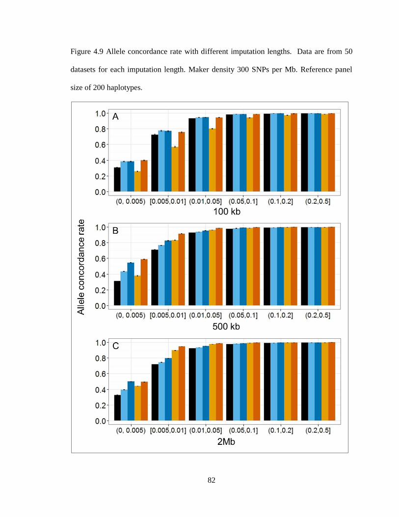
82
Figure 4.9 Allele concordance rate with different imputation lengths. Data are from 50
datasets for each imputation length. Maker density 300 SNPs per Mb. Reference panel
size of 200 haplotypes.

83
Figure 4.10 Expected heterozygote concordance rate for different imputation lengths.
Data are from 50 datasets for each imputation length. Maker density 300 SNPs per Mb.
Reference panel size of 200 haplotypes.

84
Figure 4.11 SNP discovery rate for imputations with different marker densities. Data are
from 50 datasets for each maker density. Imputation length is 1Mb. Reference panel size
of 200 haplotypes. Horizontal axis represents number of SNPs per Mb in the study
sample. A and B are the discovery rates from selected reference panels. C and D are the
discovery rate from imputed datasets.
D

85
Figure 4.12 R-square for imputations with different marker densities. Data are from 50
datasets for each maker density. Imputation length is 1Mb. Reference panel size of 200
haplotypes. Horizontal axis represents number of SNPs per Mb in the study sample. A
and B are the discovery rates from selected reference panels. C and D are the discovery
rate from imputed datasets.

86

87
Figure 4.13 Allele concordance rate for imputations with different marker density in
study samples. Data are from 50 datasets for each maker density. Imputation length is
1Mb. Reference panel size of 200 haplotypes. Horizontal axis represents number of SNPs
per Mb in the study sample. A and B are the discovery rates from selected reference
panels. C and D are the discovery rate from imputed datasets.

88

89
Figure 4.14 Expected heterozygote concordance rate for different maker density. Data are
from 50 datasets for each maker density. Imputation length is 1Mb. Reference panel size
of 200 haplotypes. Horizontal axis represents number of SNPs per Mb in the study
sample. A and B are the discovery rates from selected reference panels. C and D are the
discovery rate from imputed datasets.

90

91
Figure 4.15 SNP discovery rate for the 1000 Genomes data. Data are from ten regions of
1 Mb from chromosome 20 of EUR ancestry. For a total 381 diploid individuals, select
160 haplotypes as a reference panel. Horizontal axis is the MAF group.

92
Figure 4.16 R-square for imputations of the 1000 Genomes data. Data are from ten
regions of 1 Mb from chromosome 20 of EUR ancestry. For a total 381 diploid
individuals, select 160 haplotypes as a reference panel. Horizontal axis is the MAF group.

93
Figure 4.17 Allele concordance rate for the 1000 Genomes data. Data are from ten
regions of 1 Mb from chromosome 20 of EUR ancestry. For a total 381 diploid
individuals, select 160 haplotypes as a reference panel. Horizontal axis is the MAF group.

94
Figure 4.18 Expected heterozygote concordance rate for the 1000 Genomes data. Data
are from ten regions of 1 Mb from chromosome 20 of EUR ancestry. For a total 381
diploid individuals, select 160 haplotypes as a reference panel. Horizontal axis is the
MAF group.

95
Chapter 5 Conclusion
The technological advancements allow investigators to use next-generation sequencing
data to identify rare genetic variants for complex diseases. However, association tests of
rare variants require a large sample size to obtain enough counts of the minor alleles to
gain sufficient statistical power and it is still expensive to sequence a large sample.
Genotype imputation can augment sequence data while challenges still remain, such as
imputations of data with population or family structures and imputations of rare variants.
In this dissertation I develop an approach to apply genotype imputation to family-based
data and propose two sampling strategies based on existing array data for planning
sequencing studies with limited budgets.
In Chapter 2, I propose a novel strategy for imputing family-based genotype data in an
association study for bipolar disorder, with the aim to fine mapping risk loci that
contribute to a previous observed linkage peak at 8q24. Using about 3,000 SNPs across
the region in 3,512 individuals from 737 families with European ancestry including the
families used in previous linkage analysis, I perform a detailed single-maker analysis
under different genetic models. In addition, I impute the genotypes for all the HapMap
markers in the assayed region. The results show marginal significance of loci near three
genes.

96
The reasons for no statistically significant signals found might be multifold. First, bipolar
disorder is a highly heterogeneous disease, both phenotypically and genetically. Second,
the limitations of the software on complex family structures may also reduce power in the
analysis. Third, there may be no risk loci in the studied region.
Future directions for this project involve further characterizing the disease features and
identifying more variants in the region through sequencing. Because of the high
heterogeneity of bipolar disorder, selecting a clinically more homogeneous subset of
patients might increase the power to detect risk loci that contribute to a certain pathway.
For example, one can select only patients diagnosed with bipolar I disorder, or bipolar
patients who also have anxiety disorder (Saunders et al. 2009; Saunders et al. 2012). In
addition, one can identify the estimated number of shared haplotypes at 8q24 in the
sample and sequence individuals who carry those shared haplotypes. Once new rare
variants are identified in this region, one can test associations of these novel rare variants
with bipolar disorder using the entire study sample or other samples through cost-
effective customized arrays.
In Chapter 3 and Chapter 4, I investigate on how to use genotype imputation when
planning sequencing studies by proposing two sampling strategies based on genotypes
from existing array data. The goal is to find an optimal subset to sequence, in a sense that
one can identify the maximal number of variants via sequencing the selected subset, and
obtaining the maximal imputation accuracy when using the sequenced subset as a
reference panel to get the sequences of the entire study sample. In Chapter 3, I focus on

97
the property of the selected panel only and aim to make the selected haplotypes to be
most distinct from each other in order to incorporate the maximal diversity of the sample
into the selected panel. To achieve this goal, I adapt the phylogenetic diversity and a
greedy algorithm to select the subset with the maximal subtree length (Pardi and
Goldman 2005; Steel 2005). The assumption is that the number of mutation events is
proportional to the evolutional time and the subset with maximal tree length represents
the longest evolutionary time. In Chapter 4, I consider both the selected haplotypes and
the unselected haplotypes when identifying the optimal panel. I propose another sampling
strategy for sequencing studies, termed as the most representative subset. The goal is to
select a subset such that every unselected haplotype in the study sample has at least one
similar haplotype in the selected subset that can be used as its template in imputation.
In summary, I present two sampling strategies for planning sequence studies. Both
strategies provide better performance than randomly selected samples. Both methods
allow for incorporating other selection criteria. For example, one can treat individuals
selected from other criteria as an initial set and apply the algorithm to the initial set as an
extension. Based on the results from the simulated data as well as the real sequence data
from the 1000 Genomes Project, I recommend a few guidelines which strategy
investigators can choose in order to identify maximal polymorphic sites from a study
sample when planning sequencing studies with existing genotype data: 1) For study
individuals that are from one population, the representative reference panel is more likely
to provide a better performance. 2) For study individuals that are from closely related
populations, the diverse reference panel is more likely to provide a better performance. 3)

98
The diverse panel might work better than the representative panel when imputing short
regions (e.g., regions of a few hundred kbs), whereas the representative panel might work
better when imputing longer regions, e.g., a few Mbs or longer. 4) The differences
between reference panels become smaller when more individuals are sequenced.
Future work for the most diverse reference panel involves better characterizing the data
on which the algorithm can work best. For example, Bordewich et al. (2008) found that
selecting the most diverse subset may not always be the best choice in certain tree
topologies and proposed an alternative strategy. However, they did not provide a
systemic measure to categorize the tree topologies. One can better use the algorithm if
there is a summary statistics that provides such information. Future work for the most
representative panel involves algorithm optimization. The hill-climbing based approach is
easy to implement and takes limited memory. But it is often not efficient in finding a
solution and the solution may not be globally optimal. I intend to further optimize the
algorithm by borrowing ideas from tag SNPs selection as its idea is similar as the most
representative panel.
Future directions for both panels include 1) further characterizing the two sampling
strategies in order to determine when they work the best. My goal is to provide guidelines
for investigators to select a subset to sequence when they plan sequencing studies. Based
on simulation results, I have provided several suggestions on which sampling strategy to
use with a specific study sample. In general, the most diverse algorithm aims to maximize
variants discovery while the representative algorithm aims to find the maximal

99
imputation accuracy. I intend to characterize the study samples from population genetics
perspective to see if there exists some summary statistics of a study sample that can be
used to select the best panel for the specific study sample. 2) Quantifying the gain by
using the proposed panels than a randomly selected panel, either economically and
statistically. 3) Combining existing sequence data such as the data from the 1000
Genomes Project when selecting the optimal reference panel. For example, one can
identify a subset of the study sample that shares common fragments with sequences from
the 1000 Genomes Project and get the sequences the selected subset by imputation using
data from the 1000 Genomes Project as references, while sequencing the rest of the study
sample that are more different from the sequences from the 1000 Genomes Project. 4)
Incorporating phenotype information. Ignoring phenotype information in selecting a
subset to sequence may bias the downstream disease association tests. One can avoid the
problem by considering sequencing as a SNP discovery step and get genotypes for the
entire study sample or other samples through more cost-effective customized arrays for
association tests. Answering these questions and better characterizing the two strategies
will certainly provide investigators more information in choosing the optimal strategy to
use when planning sequencing studies in the future.
In summary, in this dissertation, I have addressed challenges and have provided strategies
in applying genotype imputation to data with family structures and to augment sequence
data in next-generation sequencing studies. These strategies provide practical solutions to
the problems arising from identifying risk variants, especially rare risk variants for
complex diseases. I have presented results in applying one of my proposed methods to

100
bipolar disorder, but all the proposed methods can be applied to other common complex
disorders. Currently thoughts of GWAS have been performed with millions of individuals
involved. I expect that investigators have started to sequence them and will eventually get
the sequences for all these individuals with phenotypes of interest either by direct
sequencing or high quality imputation. My dissertation work thus has the potential to
provide investigators a cost-effective way in get the high quality sequences of a large
study sample with limited budget.

101
Bibliography
Askland K, Read C, J M. 2009. Pathways-based analyses of whole-genome association
study data in bipolar disorder reveal genes mediating ion channel activity and
synaptic neurotransmission. Hum Genet 125(1) (1): 63-79.
Avramopoulos D, Willour VL, Zandi PP, Huo Y, MacKinnon DF, Potash JB, DePaulo
JR, Jr., McInnis MG. 2004. Linkage of bipolar affective disorder on chromosome
8q24: follow-up and parametric analysis. Mol Psychiatry 9(2): 191-196.
Badner JA, Gershon ES. 2002. Meta-analysis of whole-genome linkage scans of bipolar
disorder and schizophrenia. Mol Psychiatry 7(4): 405-411.
Barnett JH, Smoller JW. 2009. The genetics of bipolar disorder. Neuroscience 164(1):
331-343.
Bodmer W, Bonilla C. 2008. Common and rare variants in multifactorial susceptibility to
common diseases. Nat Genet 40(6): 695-701.
Bordewich M, Rodrigo AG, Semple C. 2008. Selecting taxa to save or sequence:
desirable criteria and a greedy solution. Syst Biol 57(6): 825-834.
Brown AHD. 1989. Core collections: a practical approach to genetic resources
management. Genome 31(2): 818-824.
Browning BL, Yu Z. 2009. Simultaneous genotype calling and haplotype phasing
improves genotype accuracy and reduces false-positive associations for genome-wide
association studies. Am J Hum Genet 85(6): 847-861.
Bryant D. 2005. On the Uniqueness of the Selection Criterion in Neighbor-Joining. J
Classif 22(3-15).
Burmeister M, McInnis MG, Zöllner S. 2008. Psychiatric genetics: progress amid
controversy. Nat Rev Genet 9(7): 527-540.
Carter CJ. 2007. Multiple genes and factors associated with bipolar disorder converge on
growth factor and stress activated kinase pathways controlling translation initiation:
implications for oligodendrocyte viability. Neurochem Int 50(3): 461-490.

102
Chumakov I, Cohen D, Macciardi F. 2006. Compositions and methods for treating mental
disorders. US.
Cichon S, Schumacher J, Muller DJ, Hurter M, Windemuth C, Strauch K, Hemmer S,
Schulze TG, Schmidt-Wolf G, Albus M et al. 2001. A genome screen for genes
predisposing to bipolar affective disorder detects a new susceptibility locus on 8q.
Hum Mol Genet 10(25): 2933-2944.
Cirulli ET, Goldstein DB. 2010. Uncovering the roles of rare variants in common disease
through whole-genome sequencing. Nat Rev Genet 11(6): 415-425.
Cohen JC, Kiss RS, Pertsemlidis A, Marcel YL, McPherson R, Hobbs HH. 2004.
Multiple rare alleles contribute to low plasma levels of HDL cholesterol. Science
305(5685): 869-872.
De Mooij-van Malsen AJ, van Lith HA, Oppelaar H, Hendriks J, de Wit M, Kostrzewa E,
Breen G, Collier DA, Olivier B, Kas MJ. 2009. Interspecies trait genetics reveals
association of Adcy8 with mouse avoidance behavior and a human mood disorder.
Biol Psychiatry 66(12): 1123-1130.
Dick DM, Foroud T, Flury L, Bowman ES, Miller MJ, Rau NL, Moe PR, Samavedy N,
El-Mallakh R, Manji H et al. 2003. Genomewide linkage analyses of bipolar disorder:
a new sample of 250 pedigrees from the National Institute of Mental Health Genetics
Initiative. Am J Hum Genet 73(1): 107-114.
Endicott J, Spitzer RL. 1978. A diagnostic interview: the schedule for affective disorders
and schizophrenia. Arch Gen Psychiatry 35(7): 837-844.
Faith DP. 1992. Conservation evaluation and phylogenetic diversity. Biol Conserv 61: 1-
10.
Ferreira MA, O'Donovan MC, Meng YA, Jones IR, Ruderfer DM, Jones L, Fan J, Kirov
G, Perlis RH, Green EK et al. 2008. Collaborative genome-wide association analysis
supports a role for ANK3 and CACNA1C in bipolar disorder. Nat Genet 40(9): 1056-
1058.
Frazer KA Ballinger DG Cox DR Hinds DA Stuve LL Gibbs RA Belmont JW Boudreau
A Hardenbol P Leal SM et al. 2007. A second generation human haplotype map of
over 3.1 million SNPs. Nature 449(7164): 851-861.
Fridley BL, Jenkins G, Deyo-Svendsen ME, Hebbring S, Freimuth R. 2010. Utilizing
genotype imputation for the augmentation of sequence data. PloS One 5(6): e11018.
Gargus JJ. 2006. Ion channel functional candidate genes in multigenic neuropsychiatric
disease. Biol Psychiatry 60(2): 177-185.
Gibson G. 2011. Rare and common variants: twenty arguments. Nat Rev Genet 13(2):
135-145.

103
Gopalakrishnan S, Qin ZS. 2006. TagSNP selection based on pairwise LD criteria and
power analysis in association studies. Pac Symp Biocomput: 511-522.
Hao K, Chudin E, McElwee J, Schadt EE. 2009. Accuracy of genome-wide imputation of
untyped markers and impacts on statistical power for association studies. BMC Genet
10: 27.
Howie B, Fuchsberger C, Stephens M, Marchini J, Abecasis GR. 2012. Fast and accurate
genotype imputation in genome-wide association studies through pre-phasing. Nat
Genet 44(8): 955-959.
Howie BN, Donnelly P, Marchini J. 2009. A flexible and accurate genotype imputation
method for the next generation of genome-wide association studies. PLoS Genet 5(6):
e1000529.
Huang L, Jakobsson M, Pemberton TJ, Ibrahim M, Nyambo T, Omar S, Pritchard JK,
Tishkoff SA, Rosenberg NA. 2011. Haplotype variation and genotype imputation in
African populations. Genet Epidemiol 35(8): 766-780.
Huang L, Li Y, Singleton AB, Hardy JA, Abecasis G, Rosenberg NA, Scheet P. 2009.
Genotype-imputation accuracy across worldwide human populations. Am J Hum
Genet 84(2): 235-250.
Hudson RR. 2002. Generating samples under a Wright-Fisher neutral model of genetic
variation. Bioinformatics 18(2): 337-338.
Jewett EM, Zawistowski M, Rosenberg NA, Zöllner S. 2012. A coalescent model for
genotype imputation. Genetics 194(4): 1239-1255.
Jostins L, Morley KI, Barrett JC. 2011. Imputation of low-frequency variants using the
HapMap3 benefits from large, diverse reference sets. Eur J Hum Genet 19(6): 662-
666.
Kang CJ, Marjoram P. 2012. A sample selection strategy for next-generation sequencing.
Genet Epidemiol 36(7): 696-709.
Lee KW, Woon PS, Teo YY, Sim K. 2012. Genome wide association studies (GWAS)
and copy number variation (CNV) studies of the major psychoses: what have we
learnt? Neurosci Biobehav Rev 36(1): 556-571.
Li Y, Sidore C, Kang HM, Boehnke M, Abecasis GR. 2011. Low-coverage sequencing:
implications for design of complex trait association studies. Genome Res 21(6): 940-
951.
Li Y, Willer C, Sanna S, Abecasis G. 2009. Genotype imputation. Annu Rev Genomics
Hum Genet 10: 387-406.

104
Li Y, Willer CJ, Ding J, Scheet P, Abecasis GR. 2010. MaCH: using sequence and
genotype data to estimate haplotypes and unobserved genotypes. Genet Epidemiol
34(8): 816-834.
Macayran JF, Brodie SG, Rao PN, O'Connor MJ, Gray JA, Ciarimboli B, Dipple KM.
2006. Duplication 8q22.1-q24.1 associated with bipolar disorder and speech delay.
Bipolar Disord 8(3): 294-298.
Marchini J, Howie B. 2010. Genotype imputation for genome-wide association studies.
Nat Rev Genet 11(7): 499-511.
Marchini J, Howie B, Myers S, McVean G, Donnelly P. 2007. A new multipoint method
for genome-wide association studies by imputation of genotypes. Nat Genet 39(7):
906-913.
McInnis MG, Lan TH, Willour VL, McMahon FJ, Simpson SG, Addington AM,
MacKinnon DF, Potash JB, Mahoney AT, Chellis J et al. 2003. Genome-wide scan of
bipolar disorder in 65 pedigrees: supportive evidence for linkage at 8q24, 18q22,
4q32, 2p12, and 13q12. Mol Psychiatry 8(3): 288-298.
McKhann HI, Camilleri C, Berard A, Bataillon T, David JL, Reboud X, Le Corre V,
Caloustian C, Gut IG, Brunel D. 2004. Nested core collections maximizing genetic
diversity in Arabidopsis thaliana. Plant J 38(1): 193-202.
McQueen MB, Devlin B, Faraone SV, Nimgaonkar VL, Sklar P, Smoller JW, Abou
Jamra R, Albus M, Bacanu SA, Baron M et al. 2005. Combined analysis from eleven
linkage studies of bipolar disorder provides strong evidence of susceptibility loci on
chromosomes 6q and 8q. Am J Hum Genet 77(4): 582-595.
McQuillin A, Rizig M, Gurling HM. 2007. A microarray gene expression study of the
molecular pharmacology of lithium carbonate on mouse brain mRNA to understand
the neurobiology of mood stabilization and treatment of bipolar affective disorder.
Pharmacogenet Genomics 17(8): 605-617.
Merikangas KR, Akiskal HS, Angst J, Greenberg PE, Hirschfeld RM, Petukhova M,
Kessler RC. 2007. Lifetime and 12-month prevalence of bipolar spectrum disorder in
the National Comorbidity Survey replication. Arch Gen Psychiatry 64(5): 543-552.
Nee S, May RM. 1997. Extinction and the loss of evolutionary history. Science
278(5338): 692-694.
Nelson MR, Wegmann D, Ehm MG, Kessner D, St Jean P, Verzilli C, Shen J, Tang Z,
Bacanu SA, Fraser D et al. 2012. An abundance of rare functional variants in 202
drug target genes sequenced in 14,002 people. Science 337(6090): 100-104.
Nothnagel M, Ellinghaus D, Schreiber S, Krawczak M, Franke A. 2009. A
comprehensive evaluation of SNP genotype imputation. Hum Genet 125(2): 163-171.

105
Nurnberger JI, Jr., Blehar MC, Kaufmann CA, York-Cooler C, Simpson SG, Harkavy-
Friedman J, Severe JB, Malaspina D, Reich T. 1994. Diagnostic interview for genetic
studies. Rationale, unique features, and training. NIMH Genetics Initiative. Arch Gen
Psychiatry 51(11): 849-859; discussion 863-844.
Pardi F, Goldman N. 2005. Species choice for comparative genomics: being greedy
works. PLoS Genet 1(6): e71.
Pasaniuc B, Avinery R, Gur T, Skibola CF, Bracci PM, Halperin E. 2010. A generic
coalescent-based framework for the selection of a reference panel for imputation.
Genet Epidemiol 34(8): 773-782.
Pei YF, Zhang L, Li J, Deng HW. 2010. Analyses and comparison of imputation-based
association methods. PloS One 5(5): e10827.
Perez J, Tardito D, Mori S, Racagni G, Smeraldi E, Zanardi R. 2000. Abnormalities of
cAMP signaling in affective disorders: implication for pathophysiology and
treatment. Bipolar Disord 2(1): 27-36.
Reeves PA, Panella LW, Richards CM. 2012. Retention of agronomically important
variation in germplasm core collections: implications for allele mining. Theor Appl
Genet 124(6): 1155-1171.
Russell S, Norviq P. 2009. Beyond classical search. In Artificial Intelligence: A Modern
Approach, pp. 120-129. Prentice Hall.
Saitou N, Nei M. 1987. The neighbor-joining method: a new method for reconstructing
phylogenetic trees. Mol Biol Evol 4(4): 406-425.
Saunders EF, Fitzgerald KD, Zhang P, McInnis MG. 2012. Clinical features of bipolar
disorder comorbid with anxiety disorders differ between men and women. Depress
Anxiety 29(8): 739-746.
Saunders EF, Zhang P, Copeland JN, McLnnis MG, Zollner S. 2009. Suggestive linkage
at 9p22 in bipolar disorder weighted by alcohol abuse. Am J Med Genet B,
Neuropsychiatr Genet 150B(8): 1133-1138.
Schroeder BC, Kubisch C, Stein V, Jentsch TJ. 1998. Moderate loss of function of cyclic-
AMP-modulated KCNQ2/KCNQ3 K+ channels causes epilepsy. Nature 396(6712):
687-690.
Scott LJ, Muglia P, Kong XQ, Guan W, Flickinger M, Upmanyu R, Tozzi F, Li JZ,
Burmeister M, Absher D et al. 2009. Genome-wide association and meta-analysis of
bipolar disorder in individuals of European ancestry. Proc Natl Acad Sci U S A
106(18): 7501-7506.
Selman B, Gomes CP. 2006. Hill-climbing Search. Encyclopedia of Cognitive Science.

106
Serretti A, Mandelli L. 2008. The genetics of bipolar disorder: genome 'hot regions,'
genes, new potential candidates and future directions. Mol Psychiatry 13(8): 742-771.
Shendure J, Ji H. 2008. Next-generation DNA sequencing. Nat Biotechnol 26(10): 1135-
1145.
Smoller JW, Finn CT. 2003. Family, twin, and adoption studies of bipolar disorder. Am J
Med Genet C Semin Med Genet 123C(1): 48-58.
Sokal R, Michener C. 1958. A statistical method for evaluating systematic relationships.
Univ Kans Sci Bull 38: 1409-1438.
Steel M. 2005. Phylogenetic diversity and the greedy algorithm. Syst Biol 54(4): 527-529.
Stewart RJ, Chen B, Dowlatshahi D, MacQueen GM, Young LT. 2001. Abnormalities in
the cAMP signaling pathway in post-mortem brain tissue from the Stanley
Neuropathology Consortium. Brain Res Bull 55(5): 625-629.
The 1000 Genomes Project Consortium. 2010. A map of human genome variation from
population-scale sequencing. Nature 467(7319): 1061-1073.
The International HapMap Consortium. 2005. A haplotype map of the human genome.
Nature 437(7063): 1299-1320.
Van Os J, Rutten BP, Poulton R. 2008. Gene-environment interactions in schizophrenia:
review of epidemiological findings and future directions. Schizophrenia bulletin
34(6): 1066-1082.
Wang JR, de Villena FP, Lawson HA, Cheverud JM, Churchill GA, McMillan L. 2012.
Imputation of single-nucleotide polymorphisms in inbred mice using local phylogeny.
Genetics 190(2): 449-458.
Wigginton JE, Abecasis GR. 2005. PEDSTATS: descriptive statistics, graphics and
quality assessment for gene mapping data. Bioinformatics 21(16): 3445-3447.
Xia J, Wang Q, Jia P, Wang B, Pao W, Zhao Z. 2012. NGS catalog: A database of next
generation sequencing studies in humans. Hum Mutat 33(6): E2341-2355.
Zandi PP, Avramopoulos D, Willour VL, Huo Y, Miao K, Mackinnon DF, McInnis MG,
Potash JB, Depaulo JR. 2007. SNP fine mapping of chromosome 8q24 in bipolar
disorder. Am J Med Genet B, Neuropsychiatr Genet 144B(5): 625-630.
Zandi PP, Zöllner S, Avramopoulos D, Willour VL, Chen Y, Qin ZS, Burmeister M,
Miao K, Gopalakrishnan S, McEachin R et al. 2008. Family-based SNP association
study on 8q24 in bipolar disorder. Am J Med Genet B, Neuropsychiatr Genet
147B(5): 612-618.

107
Zawistowski M, Gopalakrishnan S, Ding J, Li Y, Grimm S, Zöllner S. 2010. Extending
rare-variant testing strategies: analysis of noncoding sequence and imputed
genotypes. Am J Hum Genet 87(5): 604-617.
Zeggini E, Scott LJ, Saxena R, Voight BF, Marchini JL, Hu T, de Bakker PI, Abecasis
GR, Almgren P, Andersen G et al. 2008. Meta-analysis of genome-wide association
data and large-scale replication identifies additional susceptibility loci for type 2
diabetes. Nat Genet 40(5): 638-645.
Zhang P, Xiang N, Chen Y, Sliwerska E, McInnis MG, Burmeister M, Zöllner S. 2010.
Family-based association analysis to finemap bipolar linkage peak on chromosome
8q24 using 2,500 genotyped SNPs and 15,000 imputed SNPs. Bipolar Disord 12(8):
786-792.