the rise and fall and rise of of dependency theory part i - sigmod

Nonlinear Dynamics 26: 121–142, 2001.© 2001 Kluwer Academic Publishers. Printed in the Netherlands.

Subcritical Hopf Bifurcation in the Delay Equation Model forMachine Tool Vibrations

TAMÁS KALMÁR-NAGYDepartment of Theoretical and Applied Mechanics, Cornell University, Ithaca, NY 14853, U.S.A.

GÁBOR STÉPÁNDepartment of Applied Mechanics, Technical University of Budapest, H-1521 Budapest, Hungary

FRANCIS C. MOONSibley School of Aerospace & Mechanical Engineering, Cornell University, Ithaca, NY 14853, U.S.A.

(Received: 9 April 1998; accepted: 17 January 2001)

Abstract. We show the existence of a subcritical Hopf bifurcation in the delay-differential equation model of theso-called regenerative machine tool vibration. The calculation is based on the reduction of the infinite-dimensionalproblem to a two-dimensional center manifold. Due to the special algebraic structure of the delayed terms in thenonlinear part of the equation, the computation results in simple analytical formulas. Numerical simulations gaveexcellent agreement with the results.

Keywords: Hopf bifurcation, delay differential equation, center manifold, chatter.

1. Introduction

One of the most important effects causing poor surface quality in a cutting process is vibrationarising from delay. Because of some external disturbances the tool starts a damped oscillationrelative to the workpiece thus making its surface uneven. After one revolution of the workpiecethe chip thickness will vary at the tool. The cutting force thus depends not only on the currentposition of the tool and the workpiece but also on a delayed value of the displacement. Thelength of this delay is the time-period τ of one revolution of the workpiece. This is the so-called regenerative effect (see, for example, [12, 16, 19, 20]). The corresponding mathematicalmodel is a delay-differential equation. In order to study phenomena related to delay effects, asimple 1 DOF model of the tool was considered. Even though the model has only 1 DOF, thedelay term makes the phase space infinite-dimensional.

Experimental results of Shi and Tobias [15] and Kalmár-Nagy et al. [9] clearly showed theexistence of ‘finite amplitude instability’, that is unstable periodic motion of the tool aroundits asymptotically stable position related to the stationary cutting.

Recently, there has been increased interest in the subject. The Ph.D. theses of Johnson[8] and Fofana [4], and the paper of Nayfeh et al. [13] presented the analysis of the Hopfbifurcation in different models using different methods, like the method of multiple scales,harmonic balance, Floquet Theory (see also [14]) and of course, numerical simulations. Newmodels have been proposed to explain chip segmentation by Burns and Davies [1]. This high-frequency process may also affect the tool dynamics.

The aim of this paper is to give a rigorous analytical investigation of the Hopf bifurcationpresent in the regenerative machine tool vibration model using the theory and tools of the Hopf

122 T. Kalmar-Nagy et al.

Figure 1. 1 DOF mechanical model.

Bifurcation Theorem and the Center Manifold Theorem. Although these have been availablefor a long time [5, 7] the closed form calculation regarding the existence and the nature of thecorresponding Hopf bifurcation in the mathematical model is only feasible by using computeralgebra (see also [2]).

2. Mechanical Model for Tool Vibrations

Figure 1 shows a 1 DOF mechanical model of the regenerative machine tool vibration in thecase of the so-called orthogonal cutting (f denotes chip thickness). The model is the simplestone which still explains the basic stability problems and nonlinear vibrations arising in thissystem [16–18]. The corresponding Free Body Diagram (ignoring horizontal forces) is alsoshown in Figure 1. Here �l = l − l0 + x(t) where l, l0 are the initial spring length and springlength in steady-state cutting, respectively. The zero value of the general coordinate x(t) of thetool edge position is set in a way that the x component Fx of the cutting force F is in balancewith the spring force when the chip thickness f is just the prescribed value f0 (steady-statecutting). The equation of motion of the tool is clearly

mx = −s�l − Fx − cx. (1)

In steady-state cutting (x = x = x = 0)

0 = −s(l − l0) − Fx(f0) ⇒ Fx(f0) = −s(l − l0),

i.e., there is pre-stress in the spring. If we write Fx = Fx(f0)+�Fx then Equation (1) becomes

x + 2ζωnx + ω2nx = − 1

m�Fx, (2)

where ωn = √s/m is the natural angular frequency of the undamped free oscillating system,

and ζ = c/(2mωn) is the so-called relative damping factor.The calculation of the cutting force variation �Fx requires an expression of the cutting

force as a function of the technological parameters, primarily as a function of the chip thick-ness f which depends on the position x of the tool edge. The traditional models [20, 21] usethe cutting coefficient k1 derived from the stationary idea of the cutting force as an empiricalfunction of the technological parameters like the chip width w, the chip thickness f , and thecutting speed v.

A simple but empirical way to calculate the cutting force is using a curve fitted to dataobtained from cutting tests. Shi and Tobias [15] gave a third-order polynomial for the cuttingforce (similar to Figure 2). The coefficient of the second-order term is negative which suggests

Subcritical Hopf Bifurcation in the Delay Equation Model 123

Figure 2. Cutting force and chip thickness relation.

a simple power law with exponent less than 1. Here we will use the formula given by Taylor[18]. According to this, the cutting force Fx depends on the chip thickness as

Fx(f ) = Kwf 3/4,

where the parameter K depends on further technological parameters considered to be con-stant in the present analysis. Expanding Fx into a power series form around the desired chipthickness f0 and keeping terms up to order 3 yields

Fx(f ) ≈ Kw

(f

3/40 + 3

4(f − f0)f

−1/40 − 3

32(f − f0)

2f−5/4

0 + 5

128(f − f0)

3f−9/40

).

Or, equivalently, we can express the cutting force variation �Fx = Fx(f ) − Fx(f0) as thefunction of the chip thickness variation �f = f − f0, like

�Fx(�f ) ≈ Kw

(3

4f

−1/40 �f − 3

32f

−5/40 �f 2 + 5

128f

−9/40 �f 3

). (3)

The coefficient of �f on the right-hand side of Equation (3) is usually called the cutting forcecoefficient and denoted by k1 (k1 = (3/4)Kwf

−1/40 ). Note, that k1 is linearly proportional

to the width w of the chip, so in the upcoming calculations it will serve as a bifurcationparameter. Then Equation (3) can be rewritten as

�Fx(�f ) ≈ k1�f − 1

8

k1

f0�f 2 + 5

96

k1

f 20

�f 3.

Even though only the local bifurcation at f = f0 ⇔ �f = 0 will be investigated in this studywe mention the case when the tool leaves the material, that is f < 0 ⇔ �f < −f0. In thiscase

�Fx(�f ) = −Fx(f0)

and so the regenerative effect is ‘switched off’ until the tool makes contact with the workpieceagain.

The chip thickness variation �f can easily be expressed as the difference of the presenttool edge position x(t) and the delayed one x(t − τ) in the form

�f = x(t) − x(t − τ) = x − xτ ,


where the delay τ = 2π/� is the time period of one revolution with � being the constantangular velocity of the rotating workpiece. By bringing the linear terms to the left-hand side,Equation (2) becomes

x + 2ζωnx +(ω2

n + k1

m

)x − k1

mxτ

= k1

8f0m

((x − xτ )

2 − 5

12f0(x − xτ )

3

).

Let us introduce the nondimensional time t and displacement x

t = ωnt, x = 5

12f0x,

and the nondimensional bifurcation parameter p = k1/(mω2n) (note that the nondimensional

time delay is τ = ωnτ ). Dropping the tilde we arrive at

x + 2ζ x + (1 + p)x − pxτ = 3p

10((x − xτ )

2 − (x − xτ )3).

This second-order equation is transformed into a two-dimensional system by introducing

x(t) =(

x1(t)

x2(t)

)=(

x(t)

x(t)

)and we obtain the delay-differential equation

x(t) = L(p)x(t) + R(p)x(t − τ) + f(x(t), p), (4)

where the dependence on the bifurcation parameter p is also emphasized:

L(p) =(

0 1−(1 + p) −2ζ

),

R(p) =(

0 0p 0

),

f(x(t), p) = 3p

10

(0

(x1(t) − x1(t − τ))2 − (x1(t) − x1(t − τ))3

). (5)

3. Linear Stability Analysis

The characteristic function of Equation (4) can be obtained by substituting the trial solutionx(t) = c exp(λt) into its linear part:

D(λ, p) = det(λI − L(p) − R(p) e−λτ )

= λ2 + 2ζλ + (1 + p) − p e−λτ . (6)


Figure 3. Stability chart.

The necessary condition for the existence of a nonzero solution is

D(λ, p) = 0.

On the stability boundary shown in Figure 3 the characteristic equation has one pair ofpure imaginary roots (except the intersections of the lobes, where it has two pairs of imaginaryroots). To find this curve, we substitute λ = iω, ω > 0 into Equation (6).

D(iω, p) = 1 + p − ω2 − p cos ωτ + i(2ζω + p sinωτ) = 0.

This complex equation is equivalent to the two real equations

1 − ω2 + p(1 − cos ωτ) = 0, (7)

2ζω + p sinωτ = 0. (8)

The trigonometric terms in Equations (7) and (8) can be eliminated to yield

p = (1 − ω2)2 + 4ζ 2ω2

2(ω2 − 1).

Since p > 0 this also implies ω > 1.With the help of the trigonometric identity

1 − cosωτ

sinωτ= tan

ωτ

2

τ can be expressed from Equations (7) and (8) as

τ = 2

ω

(jπ − arctan

ω2 − 1

2ζω

), j = 1, 2, . . . ,

where j corresponds to the j th ‘lobe’ (parameterized by ω) from the right in the stabilitydiagram (j must be greater than 0, because τ > 0). And finally

� = 2π

τ= ωπ

jπ − arctan ω2−12ζω

, j = 1, 2, . . . .


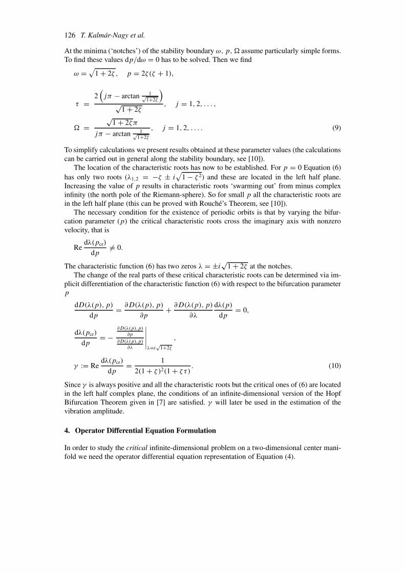
At the minima (‘notches’) of the stability boundary ω, p, � assume particularly simple forms.To find these values dp/dω = 0 has to be solved. Then we find

ω = √1 + 2ζ , p = 2ζ(ζ + 1),

τ =2(jπ − arctan 1√

1+2ζ

)√

1 + 2ζ, j = 1, 2, . . . ,

� =√

1 + 2ζπ

jπ − arctan 1√1+2ζ

, j = 1, 2, . . . . (9)

To simplify calculations we present results obtained at these parameter values (the calculationscan be carried out in general along the stability boundary, see [10]).

The location of the characteristic roots has now to be established. For p = 0 Equation (6)has only two roots (λ1,2 = −ζ ± i

√1 − ζ 2) and these are located in the left half plane.

Increasing the value of p results in characteristic roots ‘swarming out’ from minus complexinfinity (the north pole of the Riemann-sphere). So for small p all the characteristic roots arein the left half plane (this can be proved with Rouché’s Theorem, see [10]).

The necessary condition for the existence of periodic orbits is that by varying the bifur-cation parameter (p) the critical characteristic roots cross the imaginary axis with nonzerovelocity, that is

Redλ(pcr)

dp�= 0.

The characteristic function (6) has two zeros λ = ±i√

1 + 2ζ at the notches.The change of the real parts of these critical characteristic roots can be determined via im-

plicit differentiation of the characteristic function (6) with respect to the bifurcation parameterp

dD(λ(p), p)

dp= ∂D(λ(p), p)

∂p+ ∂D(λ(p), p)

∂λ

dλ(p)

dp= 0,

dλ(pcr)

dp= −

∂D(λ(p),p)

∂p

∂D(λ(p),p)

∂λ

∣∣∣∣∣λ=i

√1+2ζ

,

γ := Redλ(pcr)

dp= 1

2(1 + ζ )2(1 + ζ τ). (10)

Since γ is always positive and all the characteristic roots but the critical ones of (6) are locatedin the left half complex plane, the conditions of an infinite-dimensional version of the HopfBifurcation Theorem given in [7] are satisfied. γ will later be used in the estimation of thevibration amplitude.

4. Operator Differential Equation Formulation

In order to study the critical infinite-dimensional problem on a two-dimensional center mani-fold we need the operator differential equation representation of Equation (4).


This delay-differential equation can be expressed as the abstract evolution equation [2, 6,11] on the Banach space H of continuously differentiable functions u : [−τ, 0] → R

2

xt = Axt + F (xt ). (11)

Here xt (ϕ) ∈ H is defined by the shift of time

xt (ϕ) = x(t + ϕ), ϕ ∈ [−τ, 0]. (12)

The linear operator A at the critical value of the bifurcation parameter assumes the form

Au(ϑ) ={ d

dϑ u(ϑ), ϑ ∈ [−τ, 0),Lu(0) + Ru(−τ), ϑ = 0,

while the nonlinear operator F can be written as

F (u)(ϑ) =

0, ϑ ∈ [−τ, 0),

3p10

(0

(u1(0) − u1(−τ))2 − (u1(0) − u1(−τ))3

), ϑ = 0,

where u ∈ H (cf. Equation (5)).The adjoint space H∗ of continuously differentiable functions v : [0, τ ] → R

2 with theadjoint operator

A∗v(σ ) ={ − d

dσ v(σ ), σ ∈ (0, τ ],L∗v(0) + R∗v(τ ), σ = 0,

is also needed as well as the bilinear form ( , ) : H∗ × H → R defined by

(v,u) = v∗(0)u(0) +0∫

−τ

v∗(ξ + τ)Ru(ξ) dξ. (13)

The formal adjoint and the bilinear form provide the basis for a geometry in which it is possi-ble to develop a projection using the basis eigenvectors of the formal adjoint. The significanceof this projection is that the critical delay system has a two-dimensional attractive subsystem(the center manifold) and the solutions on this manifold determine the long time behavior ofthe full system. For a heuristic argument of how these operators and bilinear form arise, seethe Appendix. The mathematically inclined can study [6].

Since the critical eigenvalues of the linear operator A just coincide with the critical char-acteristic roots of the characteristic function D(λ, p), the Hopf bifurcation arising at thedegenerate trivial solution can be studied on a two-dimensional center manifold embeddedin the infinite-dimensional phase space.

A first-order approximation to this center manifold can be given by the center subspaceof the associated linear problem, which is spanned by the real and imaginary parts s1, s2 ofthe complex eigenfunction s(ϑ) ∈ H corresponding to the critical characteristic root iω. Thiseigenfunction satisfies

As(ϑ) = iωs(ϑ),

that is

A(s1(ϑ) + is2(ϑ)) = iω(s1(ϑ) + is2(ϑ)).


Separating the real and imaginary parts yields

As1(ϑ) = −ωs2(ϑ),

As2(ϑ) = ωs1(ϑ).

Using the definition of A results the following boundary value problem

d

dϑs1(ϑ) = −ωs2(ϑ),

d

dϑs2(ϑ) = ωs1(ϑ), (14)

Ls1(0) + Rs1(−τ) = −ωs2(0),

Ls2(0) + Rs2(−τ) = ωs1(0). (15)

The general solution to the differential equation (14) is

s1(ϑ) = cos(ωϑ)c1 − sin(ωϑ)c2,

s2(ϑ) = sin(ωϑ)c1 + cos(ωϑ)c2.

The boundary conditions (15) result in a system of linear equations for some of the unknowncoefficients:(

L + cos(ωτ)R ωI + sin(ωτ)R) ( c1

c2

)= 0. (16)

The center manifold reduction also requires the calculation of the ‘left-hand side’ criticalreal eigenfunctions n1,2 of A that satisfy the adjoint problem

A∗n1(σ ) = ωn2(σ ),

A∗n2(σ ) = −ωn1(σ ).

This boundary value problem has the general solution

n1(σ ) = cos(ωσ )d1 − sin(ωσ )d2,

n2(σ ) = sin(ωσ )d1 + cos(ωσ )d2,

while the boundary conditions simplify to

(LT + cos(ωτ)R

T − ωI − sin(ωτ)RT) ( d1

d2

)= 0. (17)

With the help of the bilinear form (13), the ‘orthonormality’ conditions

(n1, s1) = 1, (n1, s2) = 0 (18)

provide two more equations.


Since Equations (16–18) do not determine the unknown coefficients uniquely (8 unknownsand 6 equations) we can choose two of them freely (so that the others will be of simple form)

c11 = 1, c21 = 0.

Then

c1 =(

10

), c2 =

(0ω

),

d1 = 2γ

(2ζ 2 + 2ζ + 1

ζ

), d2 = 2γω

(ζ

1

).

Let us decompose the solution xt (ϑ) of Equation (11) into two components y1,2 lying inthe center subspace and into the infinite-dimensional component w transverse to the centersubspace:

xt (ϑ) = y1(t)s1(ϑ) + y2(t)s2(ϑ) + w(t)(ϑ), (19)

where

y1(t) = (n1, xt ) |ϑ=0 , y2(t) = (n2, xt ) |ϑ=0 .

With these new coordinates the operator differential equation (11) can be transformed into a‘canonical form’ (see the Appendix)

y1 = (n1, xt ) = ωy2 + nT1 (0)F, (20)

y2 = (n2, xt ) = −ωy1 + nT2 (0)F, (21)

w = Aw + F (xt ) − nT1 (0)Fs1 − nT

2 (0)Fs2, (22)

where

F = F (y1(t)s1(0) + y2(t)s2(0) + w(t)(0))

and in Equation (22) the decomposition (19) should be substituted for xt . Equations (4) and(5) give rise to the nonlinear operator

F (w + y1s1 + y2s2)(ϑ)

=

0, ϑ ∈ [−τ, 0),

35ζz

(0

z1+ζ

+ 2(w1(0) − w1(−τ)) −(

z1+ζ

)2

), ϑ = 0,

(23)

where z = y1 −ωy2 and the terms of fourth or higher order were neglected (since w(y1, y2) issecond order in Equation (24) and the normal form (35) will only contain terms up to thirdorder).


5. Two-Dimensional Center Manifold

The center manifold is tangent to the plane y1, y2 at the origin, and it is locally invariant andattractive to the flow of system (11). Since the nonlinearities considered here are nonsym-metric, we have to compute the second-order Taylor-series expansion of the center manifold.Thus, its equation can be assumed in the form of the truncated power series

w(y1, y2)(ϑ) = 1

2(h1(ϑ)y

21 + 2h2(ϑ)y1y2 + h3(ϑ)y

22). (24)

The time derivative of w can be expressed both by differentiating the right-hand side ofEquation (24) via substituting Equations (20) and (21)

w = h1y1y1 + h2y2y1 + h2y1y2 + h3y2y2

= y1(h1y1 + h2y2) + y2(h2y1 + h3y2)

= (ωy2 + d12f )(h1y1 + h2y2) + (−ωy1 + d22f )(h2y1 + h3y2)

= −ωh2y21 + ω(h1 − h3)y1y2 + ωh2y

22 + o(y3),

where f = (0 1) · F and also by calculating Equation (22)

dwdt

= Aw + F (w + y1s1 + y2s2) − (d12s1 + d22s2) f,

where

Aw ={

12 (h1y

21 + 2h2y1y2 + h3y

22 ), ϑ ∈ [−τ, 0),

Lw(0) + Rw(−τ), ϑ = 0,

Lw(0) + Rw(−τ) = 1

2y2

1(Lh1(0) + Rh1(−τ))

+ y1y2(Lh2(0) + Rh2(−τ)) + 1

2y2

2 (Lh3(0) + Rh3(−τ)).

Equating like coefficients of the second degree expressions y21 , y1y2, y2

2 we obtain a six-dimensional linear boundary value problem for the unknown coefficients h1, h2, h3

1

2h1 = −ωh2 + f11(d12s1(ϑ) + d22s2(ϑ)),

h2 = ωh1 − ωh3 + f12(d12s1(ϑ) + d22s2(ϑ)),

1

2h3 = ωh2 + f22(d12s1(ϑ) + d22s2(ϑ)), (25)

1

2(Lh1(0) + Rh1(−τ)) = −ωh2(0) + f11(d12s1(0) + d22s2(0)),

Lh2(0) + Rh2(−τ) = ωh1(0) − ωh3(0) + f12(d12s1(0) + d22s2(0)),

1

2(Lh3(0) + Rh3(−τ)) = ωh2(0) + f22(d12s1(0) + d22s2(0)), (26)


where the fij ’s denote the partial derivatives of f (with the appropriate multiplier) evaluatedat y1 = y2 = 0 (thus giving the coefficient of the corresponding quadratic term)

f11 = 1

2

∂2f

∂y21

∣∣∣∣0

, f12 = ∂2f

∂y1y2

∣∣∣∣0, f22 = 1

2

∂2f

∂y22

∣∣∣∣0

.

Introducing the following notation

h := h1

h2

h3

, C6×6 = ω

0 −2I 0I 0 −I0 2I 0

,

p = f11p0

f12p0

f22p0

, q = f11q0

f12q0

f22q0

,

p0 =(

d12

c22d22

), q0 =

(d22

−c22d12

).

Equation (25) can be written as the inhomogeneous differential equation

d

dϑh = Ch + p cos(ωϑ) + q sin(ωϑ). (27)

The general solution of Equation (27) assumes the usual form

h(ϑ) = eCϑK + M cos(ωϑ) + N sin(ωϑ). (28)

The coefficients M,N of the nonhomogeneous part are obtained after substituting this solutionback to Equation (27) resulting in a 12-dimensional inhomogeneous linear algebraic system(

C6×6 −ωI6×6

ωI6×6 C6×6

)(MN

)= −

(pq

). (29)

Since we will only need the first component w1 of w(y1, y2)(ϑ) (see Equation (23)) we haveto calculate only the first, third and fifth component of M,N,K. From Equation (29)M1

M3

M5

= −5(1 + ζ )ω

4ζγ

ω(3 + 2ζ2ζ 2 + 2ζ + 1ω(3 + 4ζ )

, (30)

N1

N3

N5

= 5(1 + ζ )ω

4ζγ

2 + 7ζ + 4ζ 2

−ζω

2ζ 2 − ζ − 2

. (31)

The boundary condition for h associated with Equation (27) comes from those parts of Equa-tion (22) where A,F are defined at ϑ = 0. It is

Ph(0) + Qh(−τ) = p + r (32)


with

P6×6 = L 0 0

0 L 00 0 L

− C6×6, Q6×6 = R 0 0

0 R 00 0 R

,

r = −( 0 f11 0 f12 0 f22)T

.

K is found by substituting the general solution (28) into Equation (32)

(P + Q e−τC)K = r + p − PM − Q(cos(ωτ)M − sin(ωτ)N). (33)

Despite its hideous look Equation (33) simplifies, because

p − PM − Q(cos(ωτ)M − sin(ωτ)N) = 0.

For our system K1

K3

K5

= 6ζ

5(9 + 33ζ + 32ζ 2)

9 + 32ζ + 32ζ 2

ω(3 + 4ζ )9 + 34ζ + 32ζ 2

. (34)

Finally, Equations (30, 31, 34) are substituted into Equation (28) resulting in the second-order approximation of the center manifold (24). It is not necessary to express the centermanifold approximation in its full form, since we only need the values of its components atϑ = 0 and −τ in the transformed operator equation (20, 21, 22). For example,

w1(0) = 1

2((M1 + K1)y

21 + 2(M3 + K3)y1y2 + (M5 + K5)y

22),

while the expression for w1(−τ) is somewhat more lengthy.

6. The Hopf Bifurcation

In order to restrict a third-order approximation of system (20–22) to the two-dimensionalcenter manifold calculated in the previous section, the second-order approximation w(y1, y2)

of the center manifold has to be substituted into the two scalar equations (20) and (21). Thenthese equations will assume the form

y1 = ωy2 + a20y21 + a11y1y2 + a02y

22 + a30y

31 + a21y

21y2 + a12y1y

22 + a03y

32 ,

y2 = −ωy1 + b20y21 + b11y1y2 + b02y

22 + b30y

31 + b21y

21y2 + b12y1y

22 + b03y

32 . (35)

Using 10 out of these 14 coefficients ajk, bjk , the so-called Poincaré–Lyapunov constant �

can be calculated as shown in [5] or [7]

� = 1

8ω[(a20 + a02)(−a11 + b20 − b02) + (b20 + b02)(a20 − a02 + b11)]

+ 1

8(3a30 + a12 + b21 + 3b03).


The negative/positive sign of � determines if the Hopf bifurcation is supercritical or subcriti-cal. Despite the above described tedious calculations � is quite simple:

� = 9ζγ

50

45 + 177ζ + 196ζ 2 + 24ζ 3

9 + 33ζ + 32ζ 2> 0.

This means that the Hopf bifurcation is subcritical, that is unstable periodic motion existsaround the stable steady state cutting for cutting coefficients p which are somewhat smallerthan the critical value pcr. This unstable limit cycle determines the domain of attraction of theasymptotically stable stationary cutting.

The estimation of the vibration amplitude has the simple form

r =√

− γ

�(p − pcr) =

√γpcr

�

√1 − p

pcr.

The approximation of the corresponding periodic solution of the original operator differentialequation (11) can be obtained from the definition (12) of xt as

xt (ϑ) = x(t + ϑ) = y1(t)s1(ϑ) + y2(t)s2(ϑ) + w(t)(ϑ)

≈ r(cos(ωt)s1(ϑ) − ω sin(ωt)s2(ϑ)).

The periodic solution of the delay-differential equation (4) can be obtained in the form

x(t) = xt (0) ≈ y1(t)s1(0) + y2(t)s2(0)

= r

(cos(ωt)

−ω sin(ωt)

). (36)

Since the relative damping factor ζ is usually far less than 1 in realistic machine tool struc-tures, the first-order Taylor expansion of the amplitude r with respect to ζ is also a goodapproximation

r ≈ 30 + 11ζ

9√

5

√1 − p

pcr.

Let us transform the nondimensonal time and displacement back to the original ones. Selectingthe first coordinate of Equation (36), we obtain the approximate form of the unstable periodicmotion embedded in the regenerative machine tool vibrations for p < pcr (see also [17])

x(t) ≈ 4

15√

5

30 + 11ζ

f0

√1 − p

pcrcos(ωn

√1 + 2ζ t).

7. Numerical Results

The results of the above sections were confirmed numerically. Simulations with

ζ = 0.1, j = 1

were carried out (see Equations (9)). The full delay equation (4, 5) was integrated in Math-ematica. To find the amplitude of the unstable limit cycle this equation was integrated with


Figure 4. Bifurcation diagram.

sinusoidal initial functions of different amplitudes. The growth or decay of the solution (aftersome transient) decides whether the solution is ‘outside’ or ‘inside’ of the unstable limitcycle. Using a bisection routine allows the computation of the location of the unstable limitcycle with good accuracy. The bifurcation diagram (presenting the amplitude of the unstablelimit cycle vs the normalized bifurcation parameter) is shown in Figure 4, together with theanalytical approximation (solid line). The agreement is excellent.

8. Conclusions

The existence and nature of a Hopf bifurcation in the delay-differential equation for self-excited tool vibration is presented and proved analytically with the help of the Center Manifoldand Hopf Bifurcation Theory. The simple results are due to the special structure of the nonlin-earities considered in the cutting force dependence on the chip thickness. On the other handthis analysis is local in the sense that it does not account for nonlinear phenomena as the toolleaves the material. In this case the regenerative effect disappears, and the result of the localanalysis is not valid anymore [3, 9].

Finally, the semi-analytical and numerical results of Nayfeh et al. [13] show some caseswhere a slight supercritical bifurcation appears before the birth of the unstable limit cycle, andthey present also some robust supercritical Hopf bifurcations. These results were calculatedat critical parameter values somewhat away from the ‘notches’ of the stability chart chosen inthis study. The model considered there also contained structural nonlinearities.

Appendix

CANONICAL FORM FOR ORDINARY AND DELAY DIFFERENTIAL EQUATIONS

In this Appendix we will show an analogy between ordinary and delay differential equationsthus motivating the definitions of the differential operator, its adjoint and the bilinear formused to investigate Hopf bifurcation in delay equations.

In particular it is shown that the time-delay problem leads to an operator that is the gener-alization of the defining matrix in a system of ODEs with constant coefficients.


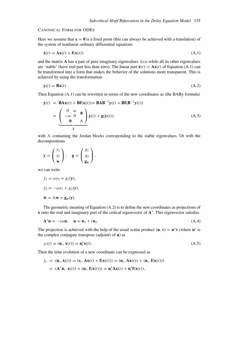
CANONICAL FORM FOR ODES

Here we assume that x = 0 is a fixed point (this can always be achieved with a translation) ofthe system of nonlinear ordinary differential equations

x(t) = Ax(t) + f(x(t)) (A.1)

and the matrix A has a pair of pure imaginary eigenvalues ±iω while all its other eigenvaluesare ‘stable’ (have real part less than zero). The linear part x(t) = Ax(t) of Equation (A.1) canbe transformed into a form that makes the behavior of the solutions more transparent. This isachieved by using the transformation

y(t) = Bx(t). (A.2)

Then Equation (A.1) can be rewritten in terms of the new coordinates as (the BABy formula)

y(t) = BAx(t) + Bf(x(t))= BAB−1y(t) + Bf(B−1y(t))

= 0 ω

−ω 00

0 1

︸︷︷︸

J

y(t) + g(y(t)), (A.3)

with 1 containing the Jordan blocks corresponding to the stable eigenvalues. Or with thedecompositions

y = y1

y2

w

, g = g1

g2

gw

,

we can write

y1 = ωy2 + g1(y),

y2 = −ωy1 + g2(y),

w = 1w + gw(y).

The geometric meaning of Equation (A.2) is to define the new coordinates as projections ofx onto the real and imaginary part of the critical eigenvector of A∗. This eigenvector satisfies

A∗n = −iωn, n = n1 + in2. (A.4)

The projection is achieved with the help of the usual scalar product (u, v) = u∗v (where u∗ isthe complex conjugate transpose (adjoint) of u) as

yi(t) = (ni , x(t)) = n∗i x(t). (A.5)

Then the time evolution of a new coordinate can be expressed as

yi = (ni , x(t)) = (si ,Ax(t) + f(x(t))) = (ni ,Ax(t)) + (ni , f(x(t)))

= (A∗ni , x(t)) + (ni , f(x(t))) = n∗i Ax(t) + n∗

i f(x(t)),


where we used the linearity of the scalar product and the identity

(u,Av) = (A∗u, v).

This result is equivalent with Equation (A.3).The coordinates y1(t), y2(t) of the linear system y(t) = Jy(t) describe stable (but not

asymptotically stable) solutions, while the other coordinates represent exponentially decayingones. In other words the linear equation

y(t) = Jy(t)

has a two-dimensional attractive invariant subspace (a plane). To obtain the two real vectorsthat span this plane we first find the two complex conjugate eigenvectors that satisfy

Js = iωs, (A.6)

Js∗ = −iωs∗. (A.7)

These are

s = 1

i

0

, s∗ = 1

−i

0

.

The two real vectors

s1 = Re s = 1

00

, s2 = Im s = 0

10

span the plane in question. n, s satisfy the orthonormality conditions

(n1, s1) = (n2, s2) = 1, (A.8)

(n1, s2) = (n2, s1) = 0. (A.9)

Note that since (n, s) = (n1, s1) + (n2, s2) + i((n2, s1) − (n1, s2)) Equations (A.8) and (A.9)are equivalent to

(n, s) = 2.

Equations (A.6) and (A.7) can also be written as

Js1 = −ωs2,

Js2 = ωs1,

which can then be solved for the real vectors.


CANONICAL FORM FOR DDES

Let us first consider a linear scalar autonomous delay differential equation (and the corre-sponding initial function) of the form

x(t) = Lx(t) + Rx(t − τ) + f (x(t), x(t − τ)),

x(t) = φ(t) t ∈ [−τ, 0). (A.10)

The first goal is to put Equation (A.10) into a form similar to Equation (A.1). Here an at-tempted numerical solution could give a clue. Discretizing Equation (A.10) leads to

dxidϑ

≈ 1

dϑ(xi−1 − xi), i = 1, . . . , N,

dxidϑ

∣∣∣∣ϑ=0

= Lx0 + RxN + f (x0, xN ).

Taking the limit dϑ → 0, and defining the ‘shift of time’ (a chunk of a function)

xt (ϑ) = x(t + ϑ),

we have the following

d

dϑxt (ϑ) = d

dϑxt (ϑ), ϑ ∈ [−τ, 0),

d

dϑxt (ϑ)

∣∣∣∣ϑ=0

= Lxt (0) + Rxt(−τ) + f (xt (0), xt (−τ)).

This motivates our definition of the linear differential operator A

Au(ϑ) ={

ddϑ u(ϑ), ϑ ∈ [−τ, 0),

Lu(0) + Ru(−τ), ϑ = 0,(A.11)

and the nonlinear operator F

F (u)(ϑ) ={

0, ϑ ∈ [−τ, 0),f (u(0)), ϑ = 0,

(A.12)

Since d/dϑ = d/dt , we can rewrite Equation (A.10) as

d

dtxt (ϑ) = xt (ϑ) = Axt (ϑ) + F (xt )(ϑ).

This operator formulation can be extended to multidimensional systems as well

xt (ϑ) = Axt (ϑ) + F (xt )(ϑ). (A.13)

This form is very similar to the system of ODEs (A.1). There is one very important difference,though. Equation (A.13) represents an infinite-dimensional system. However, the infinite-dimensional phase space of its linear part can also be split into stable, unstable and centersubspaces corresponding to eigenvalues having positive, negative and zero real part. If we


focus our attention to the case where the operator has imaginary eigenvalues, it means that Ahas an pair of complex conjugate eigenfunctions corresponding to ±iω satisfying

As(ϑ) = iωIs(ϑ), (A.14)

As∗(ϑ) = −iωIs∗(ϑ), (A.15)

where the identity operator I (this seemingly superfluous definition is intended to make ourlife easier as a bookkeping device) is defined as

Iu(θ) ={

u(θ), θ �= 0,u(0), θ = 0.

Note that Equations (A.14) and (A.15) represent a boundary value problem (because of thedefinition of A).

Introducing the real functions

s1(ϑ) = Re s(ϑ),

s2(ϑ) = Im s(ϑ).

Equations (A.14) and (A.15) can be rewritten as

As1(ϑ) = −ωIs2(ϑ),

As2(ϑ) = ωIs1(ϑ).

The two functions s1(ϑ), s2(ϑ) ‘span’ the center subspace which is tangent to the two-dimensional center manifold embedded in the infinite-dimensional phase space. With the helpof these functions we can try to define the new coordinates (similarly to Equation (A.5))

y1(t) = (n1(ϑ), xt (ϑ)),

y2(t) = (n2(ϑ), xt (ϑ)). (A.16)

where n satisfies A∗n = −iωn. The evolution of the new coordinate y1 would then be givenby

y1(t) = (n1(ϑ), xt (ϑ)) = (n1(ϑ),Axt (ϑ) + F (xt )(ϑ))

= (A∗n1(ϑ), xt (ϑ)) + (n1(ϑ),F (xt )(ϑ)).

Two questions arise immediately: how shall we define the pairing (., .) and what is the adjointoperator A∗? To answer the first question we can first try to use the usual inner product in thespace of continously differentiable functions on [−τ, 0)

(u(ϑ), v(ϑ)) =0∫

−τ

u∗(ϑ)v(ϑ) dϑ. (A.17)

However, we also want to include the ‘boundary terms’ at ϑ = 0 from Equations (A.11) and(A.12) so we can try to modify Equation (A.17) as

(u(ϑ), vt (ϑ)) =0∫

−τ

u∗(ϑ)v(ϑ) dϑ + u∗(0)v(0). (A.18)


Now we try to find the adjoint operator from the definition

(A∗u, v) = (u,Av)

(A∗u, v) =0∫

−τ

A∗uv dϑ + [A∗u(0)]∗v(0), (A.19)

(u,Av) =0∫

−τ

u∗Av dϑ + u∗(0)Av(0)

by parts= −0∫

−τ

d

dϑu∗v dϑ + u∗(ϑ)v(ϑ)|0−τ + u∗(0)[Lv(0) + Rv(−τ)]

= −0∫

−τ

d

dϑu∗v dϑ + u∗(0)v(0) − u∗(ϑ)v(ϑ)|−τ

+ u∗(0)Rv(−τ) + u∗(0)Lv(0)

=0∫

−τ

(− d

dϑ

)u∗vdϑ + [(I + L)∗u(0)]∗v(0)

− u∗(−τ)v(−τ) + u∗(0)Rv(−τ). (A.20)

The first two terms of Equation (A.20) are similar to those in Equation (A.19) so we seek toeliminate u∗(0)Rv(−τ) − u∗(−τ)v(−τ). Since this term is usually nonzero, we can try tomodify Equation (A.18) to get u∗(0)Rv(−τ) − u∗(τ − τ)Rv(−τ) = 0 instead. This can beachieved with the modification

(u(ϑ), v(ϑ)) =0∫

−τ

u∗(ϑ + τ)Rv(ϑ) dϑ + u∗(0)v(0). (A.21)

Using Equation (A.21)

(u,Av) = −0∫

−τ

d

dϑu∗(ϑ + τ)Rv(ϑ) dϑ + [L∗u(0) + R∗u(τ )]∗v(0).

Defining γ = ϑ + τ

(u,Av) = (A∗u, v)

=τ∫

0

(− d

dγ

)u∗(γ )Rv(γ − τ) dγ + [L∗u(0) + R∗u(τ )]∗v(0)


gives the definition of the adjoint operator

A∗u(γ ) ={ − d

dγ u(γ ), γ ∈ (0, τ ],L∗u(0) + R∗u(τ ), γ = 0,

with the two complex conjugate eigenfunctions

A∗n(γ ) = −iωIn(γ ), (A.22)

A∗n∗(γ ) = iωIn∗(γ ). (A.23)

Introducing the real functions

n1 (γ ) = Re n(γ ),

n2 (γ ) = Im n(γ ).

Equations (A.22) and (A.23) can be rewritten as

A∗n1(γ ) = ωIn2(γ ),

A∗n2(γ ) = −ωIn1(γ ).

Since Equation (A.21) requires functions from two different spaces (C1[−1,0] and C1

[0,1]) it isa bilinear form instead of an inner product. The ‘orthonormality’ conditions (see Equations(A.8) and (A.9)) are

(n1, s1) = (n2, s2) = 1,

(n2, s1) = (n1, s2) = 0.

The new coordinates y1, y2 can be found by the projections (instead of Equation (A.16))

y1(t) = y1t (0) = (n1, xt )|ϑ=0,

y2(t) = y2t (0) = (n2, xt )|ϑ=0.

Now xt (ϑ) can be decomposed as

xt (ϑ) = y1(t)s1(ϑ) + y2(t)s2(ϑ) + w(t)(ϑ) (A.24)

and the operator differential equation (A.13) can be transformed into the ‘canonical form’

y1 = (n1, xt )|ϑ=0 = (n1,Axt + F (xt ))|ϑ=0

= (n1,Axt )|ϑ=0 + (n1,F (xt ))|ϑ=0

= (A∗n1, xt )|ϑ=0 + (n1,F (xt ))|ϑ=0

= ω(n2, xt )|ϑ=0 + (n1,F (xt ))|ϑ=0 = ωy2 + nT1 (0)F,

y2 = (n2, xt )|ϑ=0 = −ωy1 + nT2 (0),F


where F = F (y1(t)s1(0) + y2(t)s2(0) + w(t)(0)) was used and

w = d

dt(xt − y1s1 − y2s2) = Axt + F (xt ) − y1Is1 − y2Is2

= A(y1s1 + y2s2 + w) + F (xt ) − y1Is1 − y2Is2

= y1(−ωIs2) + y2(ωIs1) + Aw + F (xt )

− (ωy2 + nT1 (0)F)Is1 − (−ωy1 + nT

2 (0)F)Is2

= Aw + F (xt ) − nT1 (0)FIs1 − nT

2 (0)FIs2

={

ddϑ w − nT

1 (0)Fs1 − nT2 (0)Fs2, ϑ ∈ [−τ, 0),

Lw(0) + Rw(−τ) + F − nT1 (0)Fs1(0) − nT

2 (0)Fs2(0), ϑ = 0.

Acknowledgements

The authors would like to thank Drs Dave Gilsinn, Jon Pratt, Richard Rand and Steven Yeungfor their valuable comments.

References

1. Burns, T. J. and Davies, M. A., ‘Nonlinear dynamics model for chip segmentation in machining’, PhysicalReview Letters 79(3), 1997, 447–450.

2. Campbell, S. A., Bélair, J., Ohira, T., and Milton, J., ‘Complex dynamics and multistability in a dampedoscillator with delayed negative feedback’, Journal of Dynamics and Differential Equations 7, 1995, 213–236.

3. Doi, S. and Kato, S., ‘Chatter vibration of lathe tools’, Transactions of the American Society of MechanicalEngineers 78(5), 1956, 1127–1134.

4. Fofana, M. S., ‘Delay dynamical systems with applications to machine-tool chatter’, Ph.D. Thesis, Universityof Waterloo, Department of Civil Engineering, 1993.

5. Guckenheimer, J. and Holmes, P. J., Nonlinear Oscillations, Dynamical Systems, and Bifurcations of VectorFields, Applied Mathematical Sciences, Vol. 42, Springer-Verlag, New York, 1986.

6. Hale, J. K., Theory of Functional Differential Equations, Applied Mathematical Sciences, Vol. 3, Springer-Verlag, New York, 1977.

7. Hassard, B. D., Kazarinoff, N. D., and Wan, Y. H., Theory and Applications of Hopf Bifurcations, LondonMathematical Society Lecture Note Series, Vol. 41, Cambridge University Press, Cambridge.

8. Johnson, M. A., ‘Nonlinear differential equations with delay as models for vibrations in the machining ofmetals’, Ph.D. Thesis, Cornell University, 1996.

9. Kalmár-Nagy, T., Pratt, J. R., Davies, M. A., and Kennedy, M. D., ‘Experimental and analytical investigationof the subcritical instability in turning’, in Proceedings of the 1999 ASME Design Engineering TechnicalConferences, ASME, New York, 1999, DETC99/VIB80-10, pp. 1–9.

10. Kalmár-Nagy, T., Stépán, G., and Moon, F. C., ‘Regenerative machine tool vibrations’, in Dynamics ofContinuous, Discrete and Impulsive Systems, to appear.

11. Kuang, Y., Delay Differential Equations with Applications in Population Dynamics, Mathematics in Scienceand Engineering, No. 191, Academic Press, New York, 1993.

12. Moon, F. C., ‘Chaotic dynamics and fractals in material removal processes’, in Nonlinearity and Chaos inEngineering Dynamics, J. Thompson and S. Bishop (eds.), Wiley, New York, 1994, pp. 25–37.

13. Nayfeh, A., Chin, C., and Pratt, J., ‘Applications of perturbation methods to tool chatter dynamics’, inDynamics and Chaos in Manufacturing Processes, F. C. Moon (ed.), Wiley, New York, 1997, pp. 193–213.

14. Nayfeh, A. H. and Balachandran, B., Applied Nonlinear Dynamics, Wiley, New York, 1995.


15. Shi, H. M. and Tobias, S. A., ‘Theory of finite amplitude machine tool instability’, International Journal ofMachine Tool Design and Research 24(1), 1984, 45–69.

16. Stépán, G., Retarded Dynamical Systems: Stability and Characteristic Functions, Pitman Research Notes inMathematics, Vol. 210, Longman Scientific and Technical, Harlow, 1989.

17. Stépán, G., ‘Delay-differential equation models for machine tool chatter’, in Dynamics and Chaos inManufacturing Processes, F. C. Moon (ed.), Wiley, New York, 1997, pp. 165–191.

18. Taylor, F. W., ‘On the art of cutting metals’, Transactions of the American Society of Mechanical Engineers28, 1907, 31–350.

19. Tlusty, J. and Spacek, L., Self-Excited Vibrations on Machine Tools, Nakl CSAV, Prague, 1954 [in Czech].20. Tobias, S. A., Machine Tool Vibration, Blackie and Son, Glasgow, 1965.

the rise and fall and rise of of dependency theory part i - sigmod

Documents