The restricted Erlang-R queue: Finite-size effects inservice systems with returning customers

Johan S.H. van Leeuwaarden, Britt W.J. Mathijsen, Fiona SloothaakDepartment of Mathematics and Computer Science, Eindhoven University of Technology, P.O. Box 513, 5600 MB, Eindhoven,

{j.s.h.v.leeuwaarden,b.w.j.mathijsen,f.sloothaak}@tue.nl

Galit B. Yom-TovFaculty of Industrial Engineering and Management, Technion - Israel Institute of Technology, 32000 Haifa, Israel,

gality@tx.technion.ac.il

Motivated by health care systems with repeated services that have both personnel (nurse/physician) and

space (beds) constraints, we study a restricted version of the Erlang-R model. The space restriction policies

we consider are blocking or holding in a pre-entrant queue. We develop many-server approximations for the

system performance measures when either policy applies, and explore the connection between them. We show

that capacity allocation of both resources should be determined simultaneously, and derive the methodology

to determine it explicitly. We show that the system dynamics is captured by the fraction of needy time

in the network, and that returning customers should be accounted for both in steady-state and transient

environments. We demonstrate the application of our policies in two case-studies of resource allocation in

hospitals.

Key words : Many-server approximations, QED regime, fixed-point analysis, returns, service systems,

queueing models, health care operations, nurse staffing, beds allocation

1. Introduction

Because service systems are stochastic in nature, it is common practice to use queueing theory for

performance analyses and workforce planning. Traditionally, systems are modeled after a single

station queue, such as the M/M/s (Erlang-C), M/M/s/s (Erlang-B) or M/M/s+M (Erlang-A)

models, and fluid and diffusion approximations are used to provide insights into the process dynam-

ics. However, single station models often fail to capture the more intricate dynamics of service

networks. In a health care context, think of flows of patients in a hospital from one medical ward

to another (Armony et al. 2015), within the Emergency Department (ED) between different stages

of treatment (Huang et al. 2015), or between medical facilities (Zychlinski et al. 2016). Queueing

networks can capture the dependency between several service stages and several resources. More

specifically, we are interested in the ubiquitous feature, particularly present in health care environ-

ments, that customers during their stay in the system might require a specific resource multiple

times, e.g. physicians and nurses who treat patients several times during their stay in the medi-

1

2

cal wards (Jennings and de Vericourt 2011) or the ED (Yom-Tov and Mandelbaum 2014), while

multiple resources are limited (e.g. physicians, nurses and beds).

An often ignored yet essential feature of service networks concerns the restriction on the number

of customers that can reside in the system simultaneously. Call centers, for instance, only have a

finite number of trunk lines (Khudyakov et al. 2010), whereas in health care facilities, the number

of beds poses a constraint on the number of patients that can be admitted at the same time to a

medical unit. In such situations, two or more resources (personnel, trunk lines, beds) are restricted.

In this paper, we investigate the influence of such multiple restrictions on the network dynamics

and the required staffing policies.

The restricted Erlang-R model. The canonical model for service networks with returns is

the Erlang-R model (Yom-Tov and Mandelbaum 2014) in which customers, during their stay in

the system receive a random number of services from the same pool of servers. Yom-Tov and

Mandelbaum (2014) showed that such a simple network model can be used to determine staffing

in an Israeli ED both in stable and time-varying conditions. Nevertheless, empirical studies report

that some countries, such as the US, use a different operational mode that apply strict restrictions

on entering the ED (Song et al. 2015). In typical US EDs, a patient will not enter the ED until both

a bed and a physician are available to treat her. Those restrictions can be either physical (beds)

restrictions or managerial ones—for instance by imposing a patient-to-physician ratio. In this work,

we extend the Erlang-R model by enforcing a constraint on the maximum number of available

places inside the service facility. Our model hence incorporates two kinds of resource constraints:

servers that provide the actual service and the maximum available places inside the service system.

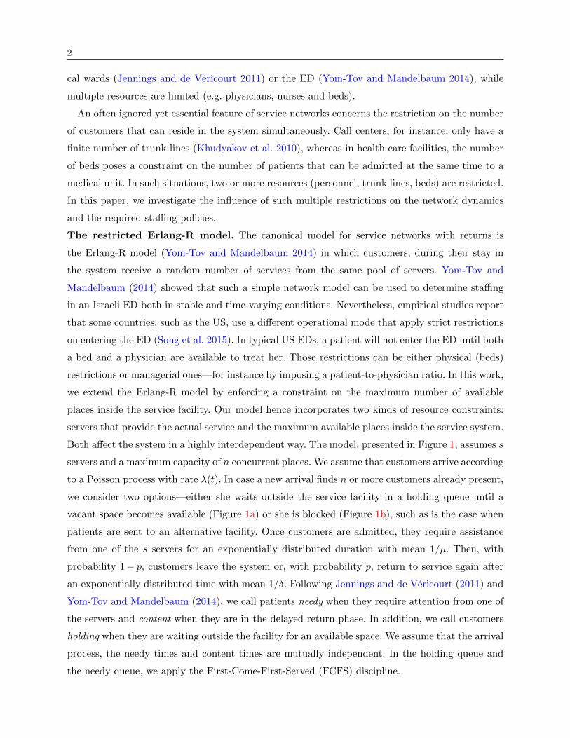
Both affect the system in a highly interdependent way. The model, presented in Figure 1, assumes s

servers and a maximum capacity of n concurrent places. We assume that customers arrive according

to a Poisson process with rate λ(t). In case a new arrival finds n or more customers already present,

we consider two options—either she waits outside the service facility in a holding queue until a

vacant space becomes available (Figure 1a) or she is blocked (Figure 1b), such as is the case when

patients are sent to an alternative facility. Once customers are admitted, they require assistance

from one of the s servers for an exponentially distributed duration with mean 1/µ. Then, with

probability 1− p, customers leave the system or, with probability p, return to service again after

an exponentially distributed time with mean 1/δ. Following Jennings and de Vericourt (2011) and

Yom-Tov and Mandelbaum (2014), we call patients needy when they require attention from one of

the servers and content when they are in the delayed return phase. In addition, we call customers

holding when they are waiting outside the facility for an available space. We assume that the arrival

process, the needy times and content times are mutually independent. In the holding queue and

the needy queue, we apply the First-Come-First-Served (FCFS) discipline.

3

s

needy

exp(µ)

∞

content

exp(δ)Arrivals

Poisson(λ)

p

1− p

nholding

(a) Erlang-R model with holding.

blocked

s

needy

exp(µ)

∞

content

exp(δ)

ArrivalsPoisson(λ)

p

1− p

n

(b) Erlang-R model with blocking.Figure 1 Restricted Erlang-R models with maximally n customers in system.

As mentioned, we consider two versions of the finite-capacity constraint. The first version is called

Erlang-R with holding, in which customers wait for an available space in the system. The second

version is called Erlang-R with blocking, in which customers meeting a full system are blocked.

Naturally, intermediate scenarios can be constructed in which a proportion of the total arrival

volume of customers indeed leaves upon finding a full system, while the rest joins the holding

room. While this paper focuses on the two extreme cases, straightforward adaptions can fit these

intermediate scenarios.

Examples of restricted Erlang-R. As noted before, an ED operated in the US can be modeled

using a restricted Erlang-R model. Another health care example are Medical Units (MU) in a

hospital. Such units specialize in specific types of illnesses (cadriatric, oncology, etc.) and have

limited resources such as nurses and beds. If the unit is full, new patients are either allocated to an

alternative medical unit, i.e. blocked, or wait for an available bed. Both policies are problematic

in terms of quality-of-care, because the personnel in the alternative unit (or the ED) may be less

knowledgable and waiting in the ED was shown to increase mortality. Moreover, ED waiting may

reduce available capacity for treating ED patients (Carmen and van Nieuwenhuyse 2016, Bennidor

and Israelit 2015), hence endangering both the delayed patient as well as others. Both the number

of personnel (nurses and physicians) and the number of beds impact service dynamics and quality-

of-care. Research so far looked at the capacity allocation of those resources separately. Green and

Yankovic (2011) and Jennings and de Vericourt (2008) looked at nurse staffing in medical units,

while de Bruin et al. (2009) looked into bed allocation. The unified model we suggest enables us to

capture the dependency between those two decisions, and its impact on other medical units in the

hospital. At the same time, we capture the two most commonly used modes of operation—blocking

and holding of new patients.

1.1. Contributions

Our main goal is to provide staffing policies for the restricted Erlang-R models that ensures high

resource utilization, while at the same time maintains a good quality-of-care. This goal relates to the

4

philosophy of the Quality-and-Efficiency-Driven (QED) regime known in many-server asymptotic

theory. We discuss the main ideas behind this regime further in §2. In this paper, we obtain

asymptotic results for the Erlang-R model with blocking in the QED regime (§4.2). Following

Jennings and de Vericourt (2008), we employ a two-fold QED staffing policy: s=R1 + β√R1 for

the number of servers and n=R1/r+ γ√R1/r for the number of customers in the system, where

β and γ are constants, R1 is the offered load of the servers and r is the fraction of time a customer

spends in the needy state. We establish limiting expressions for performance measures, such as

the probability of delay and blocking, in the form of explicit functions that depend solely on β

and γ. In deriving these limit results, we use the available product-form solution for the stationary

distribution.

Likewise, we pursue QED performance for the Erlang-R model with holding. However, a direct

analytic approach is obstructed by the absence of product-form solutions. We provide two solu-

tions for establishing QED behavior. First, we provide stochastic performance bounds that stay

meaningful in the QED regime (§3.3), which demonstrate the non-degenerate behavior of the two-

fold scaling in the large-system limit. Second, we develop a heuristic method that quantifies the

difference between the scalable holding model and the blocking model (§4.3). This is based on

the following unique approach: initially blocked patients in the blocking model are seen as if they

reattempt to get access after a some delay. The behavior of this retrial model then resembles the

Erlang-R model with blocking without retrials, yet with an increased arrival rate. The increase in

arrival rate turns out to be the solution of a fixed-point equation. Using our results on the asymp-

totic behavior of the model with blocking in the QED regime, we then obtain approximative QED

performance measures for the model with holding. Finally, we use these QED results to develop

algorithms for dimensioning and time-varying staffing (§5.1).

Using the approximations developed, numerical analysis and simulation we provide the following

managerial insights:

• We show that all resource allocation of personnel and beds should be synchronized in order to

avoid waste, and that the QED scaling provides an efficient, flexible, and easy to implement

methodology to do so.

• We conclude that reentrant customers in a restricted network are more significant than in

an open network (Erlang-R). In contrast to the open model, in which returning customers

need to be accounted for only in time-varying systems, the restricted Erlang-R model requires

explicit consideration of returning customers under stationary conditions as well.

• We show that the influence of the network structure on the system dynamics crucially depend

on the fraction of time a patient spends being needy during her stay in the system. We then

explore the influence of r on operational decisions.

5

• Combining the theoretical results, we explore the implication of managerial decisions in design-

ing an MU (§5) and an ED (§6.4). In §5, we show that enabling customers to hold in ED

before entering an MU, requires more resources both in the MU and the ED. In Section 6.4,

we compare the pros and cons of imposing strict constraints on entering an ED. We find that

size restrictions have the ability to improve the quality-of-service of the processes within the

facility, at the expense of a slight increase in pre-entrant wait and server efficiency levels.

• Finally, we show that restricting the number of admitted customers protects those customers

with complicated demand consisting of relatively many retrials/interruptions (§6.3).

When dealing with time-varying patient demands, one requires some modifications in the QED

results in order to obtain stable performance at every moment in time. We transform the two-

fold staffing policy into a time-varying one based on the Modified Offered Load (MOL) method

(§6.4). This method approximates the offered load at the needy station at each point in time via

a corresponding system with ample resources. By noting that the latter system coincides with the

Erlang-R model with ample servers, we adopt the offered load approximations given in Yom-Tov

and Mandelbaum (2014). Numerical experiments justify this method and we use this approach in

our case study §6.4.

2. Literature review

Due to increasing demand and tightening budgets in health care, there is a growing need for efficient

workforce management (Green and Savin 2008). Personnel (nurse and physician) expenditure is

one of the biggest factors in hospital costs (Kazahaya 2005), and inadequate nursing levels have

been mentioned as a significant factor in medical errors and ED overcrowding. In order to establish

appropriate nursing levels, a staffing policy requires assessment of a wide range of variables, such as

differing nurse expertise and patient acuity during the day. Current methods, such as the minimum

nurse-to-patient ratios, are often too inflexible to capture those varying conditions. The American

Hospital Association (AHA) and others call for dynamic staffing policies that can deal with the

complex and evolving nature of health care (American Hospital Association 2007). Workforce

management in health care systems has been studied extensively; see Denton (2013), Hall (2006,

2012) for overviews. In recent years it has become apparent that queueing models can be helpful

in developing staffing and routing recommendations, not just for large-scale service systems, but

also for the small and complicated health care systems.

The first to try such an approach through queueing models were Green (2006), Green and

Savin (2008) who used the single station stationary Erlang-C model to set staffing levels in EDs

and panel sizes for clinics. Using a similar approach, Bekker and de Bruin (2009) used Erlang-B

model to determine bed allocation for medical wards. The first to observe the significant impact of

6

n

p/δ

exp(µ)

∞

s

(a) The closed ward model.

λ 1− p

p

s

∞

exp(µ)

exp(δ)

(b) The Erlang-R model.

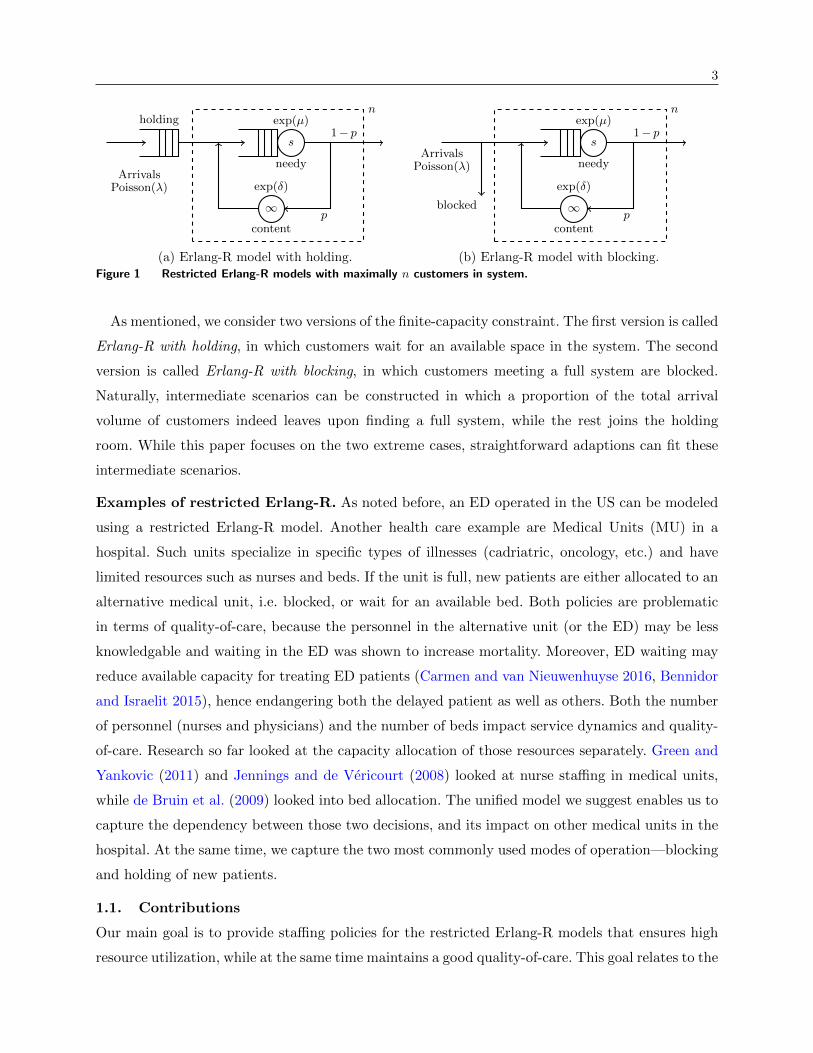
Figure 2 Two basic models with interrupted services.

interrupted services in a health care setting were Jennings and de Vericourt (2008, 2011). Motivated

by the need to set nurse-to-patient ratios for internal wards, they considered a closed queueing

system with s nurses and n beds, whuch we will refer to as the closed ward model. This is essentially

the Erlang-C model with the additional restriction that a finite population of the n patients requires

care. In their model, all beds are always occupied, and patients alternate between two phases: the

needy phase where patients require service of a nurse and the content phase where they do not; see

Figure 2a. The system dynamics of restricted Erlang-R model are equivalent to those of the closed

ward model of Jennings and de Vericourt (2008) if the holding queue would never be empty.

Campello et al. (2016) analyzed a similar operational decision, referred to as ED case manage-

ment, which determines the maximal number of patients a physician should handle in parallel.

They also used queueing networks and analyzed the stationary distribution. Note that in practice

such decision is not only affected by operational measurements such as waiting times, but also

by psychological constraints that limit physician capability to manage multiple tasks (patients)

in parallel. Diwas (2014) provided empirical evidence that physicians should not treat more than

6-7 patients at the same time. Therefore, many hospitals in the US restrict entrance to EDs even

if beds are available if physicians are overloaded. We too consider such constraints, and analyze

their impact on performance. We take a different approach than Campello et al. (2016); instead

of analyzing numerically steady-state distributions, we develop many-server approximations that

can produce insight into the system dynamics, and can be incorporated into time-varying staffing

procedures (see §6.4).

The model in Jennings and de Vericourt (2008, 2011) was developed for modeling internal

dynamics within an internal ward. However, in the ED, beds are not constantly occupied and the

utilization level depends on the flow of patients that arrive from outside the system. Yom-Tov and

Mandelbaum (2014) highlight the interrupted services while accounting for the transient nature of

patient’s arrival process, and introduced the Erlang-R model as a model for an ED. The Erlang-R

model is an open two-station queueing network that has the same layout as the restricted Erlang-R

model, except that all patients find a bed available upon arrival, see Figure 2b. In both models

7

patients experience the interrupted services, but the Erlang-R model has no further restrictions

on the bed capacity, hence neglecting the finite-size effects. Yom-Tov and Mandelbaum (2014)

showed, using a simulator tailored to an Israeli ED, that the complicated small ED dynamics

can be captured using the relatively simple Erlang-R model, and hence, its recommendations can

be implemented in ED workforce management. Although the feature of interrupted services is

present in many systems, it is particularly important for modeling EDs, because the duration of

the interruption is typically much longer than the time patients require care from a nurse. This

explains why the Erlang-R model is considered to be the canonical model for EDs. The restricted

Erlang-R model with holding/blocking thus extends the Erlang-R model with finite-size constraints

which, like interrupted services, are expected to have a decisive impact on performance.

Quality-and-Efficiency-Driven regime. The Quality-and-Efficiency driven (QED) regime for

many-server systems, also known as the Halfin-Whitt regime, adheres to a square-root staffing rule,

which is best explained for the Erlang-C model. This system can be characterized completely by

the staffing level s and the offered load R= λ/µ, which is the average workload pressure per time

unit on the system. Moreover, let ρ=R/s denote the server utilization level. Since exact analysis

provides little qualitative insight in performance with respect to the system parameters, we resort

to asymptotic analysis. This in turn provides approximations for the true system behavior. In the

QED regime (Borst et al. 2004, Halfin and Whitt 1981), the nurse utilization level is driven to

unity in accordance to (1− ρ)√s→ β as s→∞, for some fixed parameter β > 0. This gives rise

to the square-root dimensioning rule s=R+ β√R, which prescribes that the number of nurses s

exceeds the minimally required offered load R, but only by a relatively small amount β√R. As

s grows large, the probability of delay tends to a non-degenerate function that only depends on

the parameter β. This function is strictly decreasing in β > 0 with range (0,1). Consequently, any

targeted delay probability can be achieved by adjusting β. Moreover, the mean delay is of order

1/√s and hence asymptotically negligible. In this paper, we take the same approach, but determine

capacity for nurses and beds simultaneously in such a way that both the probability to wait for a

nurse and the probability to wait for a bed are non-degenerate. Moreover, the utilization of both

nurses and beds goes to unity as the size of the system increases. While the QED regime gives

precise limits when the system size (s and n in our case) goes to infinity, it is by now well known

that the asymptotic behavior kicks in quickly, so that QED limits serve as sharp approximations,

already for small systems. See Janssen et al. (2011), Zhang et al. (2012), van Leeuwaarden and

Knessl (2011, 2012), Gamarnik and Goldberg (2013), Sanders et al. (2016) for various works that

provide theoretical support for this fast relaxation.

8

1

exp(λ)

Station 0

s

exp(µ)

Station 1

1− p

p

∞

exp(δ)

Station 2

n

Figure 3 The Erlang-R model with blocking, viewed as a closed Jackson network.

In recent years, a new approach for developing approximations of performance measures of queue-

ing systems with finite-size constraints in the QED regime was suggested by van Leeuwaarden et al.

(2015, 2016). This approach characterizes the asymptotic dynamics of these analytically intractable

systems with finite-size restrictions through more tractable ones. We adopt this approach for devel-

oping the approximations for the holding model in §4.3.

3. Models and performance measures3.1. Three-dimensional Markov process

Since in the restricted Erlang-R model described the arrival process is taken Poisson, and all service

and content times are assumed independent and exponential, the system can be characterized in

terms of a Markov process. Let Q(t) = (H(t),Q1(t),Q2(t)) represent the number of patients in

the holding, needy and content state at time t, respectively. In both variants, n is the maximum

number of patients admitted to system, we have Q1(t) +Q2(t)≤ n for all t≥ 0. Due to the absence

of holding patients in the Erlang-R model with blocking, H(t) = 0 is enforced in this case, whereas

H(t) has unbounded support in the model with holding. This distinction requires us to explore the

stationary distribution of the two variants separately. Before doing so, we introduce some additional

notation. We define

R1 :=λ

(1− p)µR2 :=

pλ

(1− p)δ, (1)

where R1 and R2 can be interpreted as the offered workload brought towards the needy queue, and

the content (infinite-server) queue, respectively. Furthermore, we define

r :=δ

δ+ pµ, (2)

which is the fraction of time a patient spends in the needy state (in case she experienced no wait

during her sojourn).

9

3.1.1. Erlang-R model with blocking. In case of the blocking model, Q(t) reduces to a

finite-state Markov process Q(t) = (Q1(t),Q2(t)), where Q1(t) +Q2(t)≤ n for all t≥ 0. In fact, this

is equivalent to the closed Jackson network depicted in Figure 3 with finite population n. Station

1 in Figure 3 is an M/M/s queue with service rate µ, modeling the number of needy patients,

Q1(t). Station 2 models the number of content patients, Q2(t), and can therefore be represented as

an infinite-server queue with service rate δ. A patient can enter the unit only if Q1(t) +Q2(t)<n.

Station 0—a single-server queue—moderates this as it only produces output at rate λ in case its

queue length is positive, i.e. if n−Q1(t)−Q2(t)> 0.

Observe that because patients finding a full network are blocked, the number of patients in the

system cannot grow beyond n. Hence, the system is stable for all parameter settings, and hence a

steady-state distribution exists. Moreover, the simplification of the model with blocking allows us

to express the steady-state distribution of the system in explicit product-form. Let πb(j, k) denote

the steady-state probabilities of having j needy and k content patients in the system. Then,

πb(j, k) =

{π0

1κ(j)

1k!·Rj

1 ·Rk2 , if j+ k≤ n,

0, else,(3)

where

κ(j) :=

{j!, if j ≤ s,s!sj−s, else,

and π−10 =

∑j+k≤n

1κ(j)

1k!·Rj

1 ·Rk2 .

3.1.2. Erlang-R with holding. The Erlang-R model with holding does not lead to a Jackson

network with an elegant product-form solution for the steady-state distribution, because the holding

queue cannot be modeled as a station that is independent from the other queues in the system.

However, we are able to describe the system as a two-dimensional Markov process without loss

of information. To see this, define N := {N(t), t≥ 0} with N(t) :=H(t) +Q1(t) +Q2(t), the total

number of patients in the system (including the holding queue). Using the restriction Q1(t) +

Q2(t) ≤ n together with the fact that no bed is left vacant if a patient is waiting in the holding

queue, this yields

H(t) = (N(t)−n)+, t≥ 0,

where (·)+ := max{0, ·}. For the same reason,Q2(t) =N(t)−Q1(t) ifH(t) = 0, andQ2(t) = n−Q1(t)

otherwise. In other words,

Q2(t) = min{N(t), n}−Q1(t), t≥ 0.

Therefore, we can express the state of all three queues in the Erlang-R model with holding using

a two-dimensional Markov process X := {X(t), t≥ 0}, where

X(t) := (N(t),Q1(t)) .

10

The process X lives on the semi-infinite strip

X(t)∈ { (i, j) | j ≤min{i, n}, i∈N0, j ∈ {0,1, . . . , n}} ,

and belongs to the class of Quasi-Birth-Death (QBD) processes. The reader is referred to

Appendix A in the e-companion for a detailed description of this process, in terms of its transition

diagram and generator matrix.

Contrary to the model with blocking, the system with holding can become unstable in case

capacity is insufficient to satisfy patient demand.

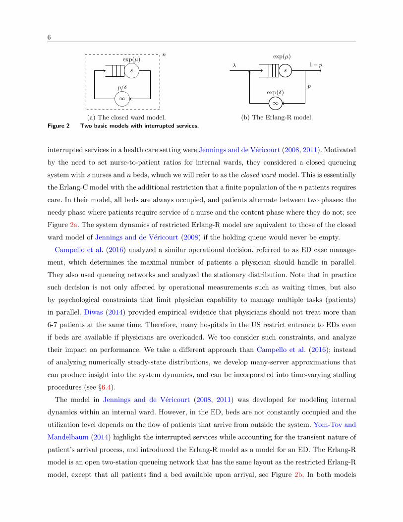
Proposition 1. The Erlang-R model with holding is stable if and only if

λ

(1− p)µs<

∑s

i=0is

(ni

)(δpµ

)i+∑n

i=s+1

(ni

)i!s!ss−i

(δpµ

)i∑s

i=0

(ni

)(δpµ

)i+∑n

i=s+1

(ni

)i!s!ss−i

(δpµ

)i =: ρmax(s,n). (4)

The proof is given in Appendix A.2 and follows from the general theory for QBD processes.

Observe that ρmax(s,n) poses an upper bound on the occupancy level of the servers in the

holding model, which is clearly smaller than 1 for all s and n. In addition, this implies that the

maximum workload Rmax(s,n) := s · ρmax(s,n) the system is able to handle is strictly less than s.

If we compare this to the open Erlang-R model, in which the maximal attainable workload equals

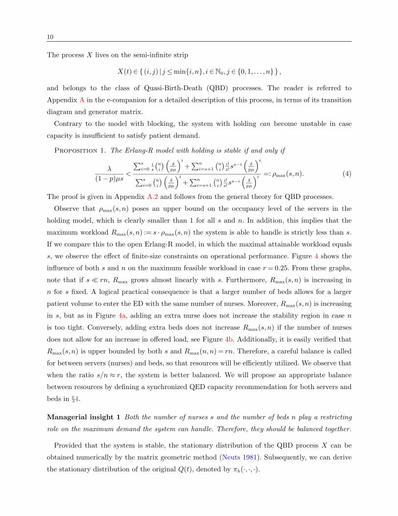
s, we observe the effect of finite-size constraints on operational performance. Figure 4 shows the

influence of both s and n on the maximum feasible workload in case r= 0.25. From these graphs,

note that if s� rn, Rmax grows almost linearly with s. Furthermore, Rmax(s,n) is increasing in

n for s fixed. A logical practical consequence is that a larger number of beds allows for a larger

patient volume to enter the ED with the same number of nurses. Moreover, Rmax(s,n) is increasing

in s, but as in Figure 4a, adding an extra nurse does not increase the stability region in case n

is too tight. Conversely, adding extra beds does not increase Rmax(s,n) if the number of nurses

does not allow for an increase in offered load, see Figure 4b. Additionally, it is easily verified that

Rmax(s,n) is upper bounded by both s and Rmax(n,n) = rn. Therefore, a careful balance is called

for between servers (nurses) and beds, so that resources will be efficiently utilized. We observe that

when the ratio s/n ≈ r, the system is better balanced. We will propose an appropriate balance

between resources by defining a synchronized QED capacity recommendation for both servers and

beds in §4.

Managerial insight 1 Both the number of nurses s and the number of beds n play a restricting

role on the maximum demand the system can handle. Therefore, they should be balanced together.

Provided that the system is stable, the stationary distribution of the QBD process X can be

obtained numerically by the matrix geometric method (Neuts 1981). Subsequently, we can derive

the stationary distribution of the original Q(t), denoted by πh(·, ·, ·).

11

0 5 10 15 200

5

10

15

20

s

Rm

ax(s,n

)

n= 20n= 40n= 60n= 80

(a) Rmax as a function of s.

0 20 40 60 80 1000

5

10

15

20

n

Rm

ax(s,n

)

s= 5s= 10s= 15s= 20

(b) Rmax as a function of n.Figure 4 The maximum achievable workload in the restricted Erlang-R model with holding for r= 0.25.

3.2. Performance measures

In this work, we concentrate on five performance measures that are central to our analysis. In

the definitions that follow, we present expressions for these measures in terms of a general three-

dimensional measure π, which one can replace by either πb or πh, depending on the scenario

considered. In the remainder of this work, we will augment the measures related to the Erlang-R

model with blocking and holding by the superscript b and h, respectively1.

As relevant performance measures, we consider the probability of holding (blocking) at enter-

ing the system, the probability of delay at the needy queue, expected waiting time for a nurse,

utilization of nurses and utilization of beds:

P(hold) =∞∑i=0

n∑j=0

π(i, j, n− j), P(delay)≈∞∑i=0

n∑j=s

n−j∑k=0

π(i, j, k), (5)

E[W ]≈∞∑i=0

n∑j=s

n−j∑k=0

max{0, j− s+ 1}µ

π(i, j, k), (6)

ρs =1

s

∞∑i=0

n∑j=0

n−j∑k=0

min{j, s}π(i, j, k), ρn =1

n

∞∑i=0

n∑j=0

n−j∑k=0

min{i, n}π(i, j, k). (7)

It should be stressed that the above expression for the delay probability and the expected waiting

time for a nurse is not exact. For the blocking model one can use the Arrival Theorem (Chen

and Yao 2001), whereby the exact expression uses n− 1 instead of n; for the holding model, the

arrival process to the needy queue, which consists of both external arrivals and content patients

becoming needy, is not Poisson. Therefore, we cannot use the PASTA argument for the holding

model. However, for both models, as we will be studying the system as s and n become large, this

approximation error will become negligible.

1 In line with H(t) = 0, we use πb(i, j, k) = πb(j, k) if i= 0, with πb(j, k) as in (3), and πb(i, j, k) = 0 otherwise, whenconsidering the model with blocking.

12

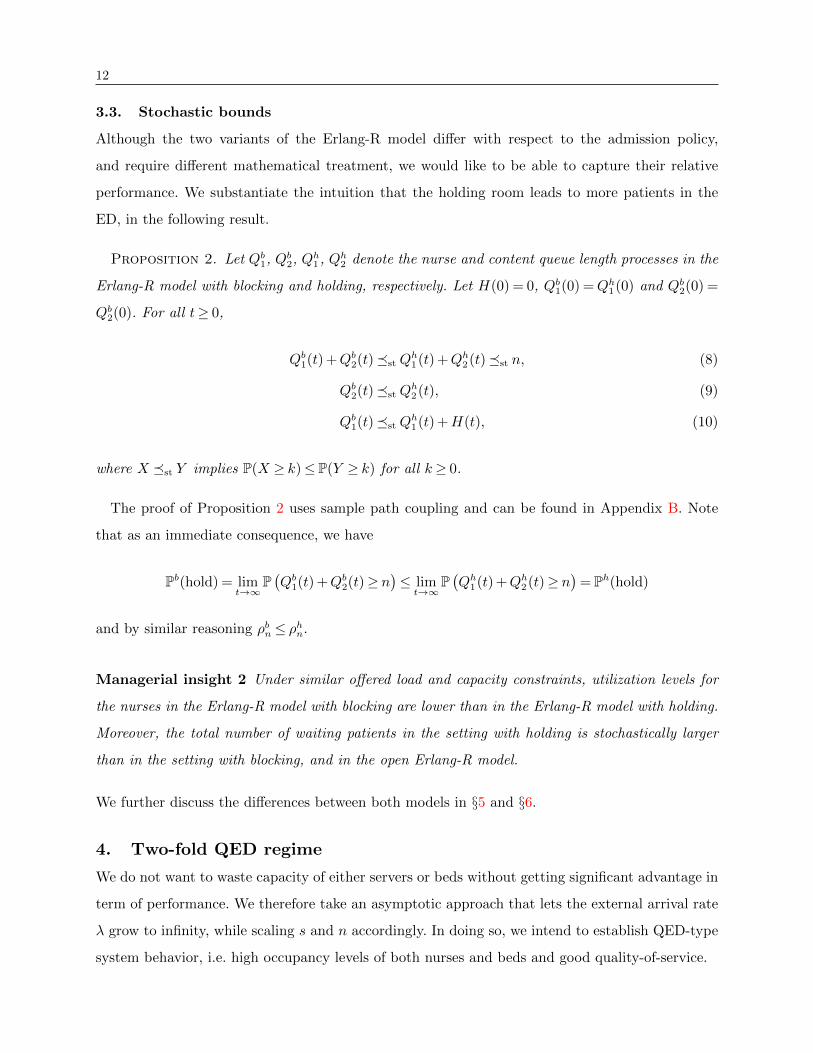
3.3. Stochastic bounds

Although the two variants of the Erlang-R model differ with respect to the admission policy,

and require different mathematical treatment, we would like to be able to capture their relative

performance. We substantiate the intuition that the holding room leads to more patients in the

ED, in the following result.

Proposition 2. Let Qb1, Qb

2, Qh1 , Qh

2 denote the nurse and content queue length processes in the

Erlang-R model with blocking and holding, respectively. Let H(0) = 0, Qb1(0) =Qh

1(0) and Qb2(0) =

Qb2(0). For all t≥ 0,

Qb1(t) +Qb

2(t)�st Qh1(t) +Qh

2(t)�st n, (8)

Qb2(t)�st Q

h2(t), (9)

Qb1(t)�st Q

h1(t) +H(t), (10)

where X �st Y implies P(X ≥ k)≤ P(Y ≥ k) for all k≥ 0.

The proof of Proposition 2 uses sample path coupling and can be found in Appendix B. Note

that as an immediate consequence, we have

Pb(hold) = limt→∞

P(Qb

1(t) +Qb2(t)≥ n

)≤ lim

t→∞P(Qh

1(t) +Qh2(t)≥ n

)= Ph(hold)

and by similar reasoning ρbn ≤ ρhn.

Managerial insight 2 Under similar offered load and capacity constraints, utilization levels for

the nurses in the Erlang-R model with blocking are lower than in the Erlang-R model with holding.

Moreover, the total number of waiting patients in the setting with holding is stochastically larger

than in the setting with blocking, and in the open Erlang-R model.

We further discuss the differences between both models in §5 and §6.

4. Two-fold QED regime

We do not want to waste capacity of either servers or beds without getting significant advantage in

term of performance. We therefore take an asymptotic approach that lets the external arrival rate

λ grow to infinity, while scaling s and n accordingly. In doing so, we intend to establish QED-type

system behavior, i.e. high occupancy levels of both nurses and beds and good quality-of-service.

13

4.1. Two-fold scaling rule

In order to identify the scaling of s and n as λ→∞, we draw inspiration from the two-fold scaling

rule in Jennings and de Vericourt (2008) and Khudyakov et al. (2010), which follows the celebrated

square-root staffing principle discussed in §2. This principle suggests that, in the most general

setting, capacity should be equal to the expected offered load entering the system, let us say R,

plus an additional variability hedge that is proportional to√R. In the restricted Erlang-R model,

we have two capacity sources, namely s and n, which experience different relevant amount of works.

The offered load the servers in the needy queue experience is given by R1, as in the regular Erlang-

R model; it does not change due to the finite-size effects, since all patients are served eventually.

Hence, we only need to account for the interrupted services. It follows that the appropriate staffing

rule for the nurses in the QED regime remains s=R1 +β√R1 for some constant β > 0.

To establish the bed capacity level, we need to reflect on the load offered to the beds. Observe that

beds remain occupied both in needy and content states. This suggests that Rn :=R1 +R2 =R1/r,

with R1 and R2 as in (1) and r the expected fraction of time a patient spends at the nurse station,

defined in (2). As a result, the appropriate staffing rule is n=Rn+γ√Rn for some constant γ > 0.

In conclusion, the two-fold QED scaling rule is given by

s =R1 +β√R1 + o(

√R1)

n = R1r

+ γ√

R1r

+ o(√R1)

(11)

with β,γ > 0 constants and R1 := λ/((1− p)µ).

Recall that we saw in Figure 4 that resources seem efficiently utilized if s/n≈ r. Scaling (11) is

in line with this reasoning since

s

n= r

(1 +

β− γ√r√

R1

+O(1/R1)

).

Remark 1. In Jennings and de Vericourt (2008), a similar scaling regime is considered, which

only relates s and n through a square-root scaling, namely the regime s = rn + γ√n, which is

equivalent to the second relation in (11) if γ = β√r−γr. Due to the absence of external arrivals in

this closed system, they let the number of beds n approach infinity as opposed to λ in our settings.

Nevertheless, this results in the same asymptotic regime.

Before turning to asymptotic expressions for the performance measures concerning the Erlang-R

model with blocking/holding, we conduct a few numerical experiments to confirm that the scaling

in (11) indeed leads to desired QED behavior.

In Figure 5 we plotted the sample paths of the three-dimensional queue length process of the

holding model in which β and γ are fixed, and R1 is increased. Observe that the needy queue

length Q1(t), plotted in orange in Figure 5, fluctuates around the values s, and stabilizes for larger

14

0 50 100 150 2000

5

10

15

20

25

t

(a) R1 = 5

0 50 100 150 2000

20

40

60

80

100

120

t

(b) R1 = 25

0 50 100 150 2000

100

200

300

400

t

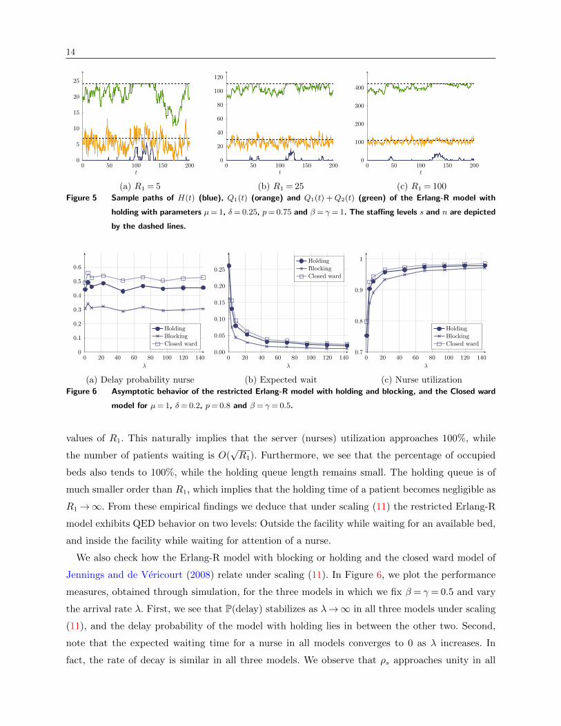
(c) R1 = 100Figure 5 Sample paths of H(t) (blue), Q1(t) (orange) and Q1(t) +Q2(t) (green) of the Erlang-R model with

holding with parameters µ= 1, δ= 0.25, p= 0.75 and β = γ = 1. The staffing levels s and n are depicted

by the dashed lines.

0 20 40 60 80 100 120 1400

0.1

0.2

0.3

0.4

0.5

0.6

λ

HoldingBlockingClosed ward

(a) Delay probability nurse

0 20 40 60 80 100 120 1400.00

0.05

0.10

0.15

0.20

0.25

λ

HoldingBlockingClosed ward

(b) Expected wait

0 20 40 60 80 100 120 1400.7

0.8

0.9

1

λ

HoldingBlockingClosed ward

(c) Nurse utilizationFigure 6 Asymptotic behavior of the restricted Erlang-R model with holding and blocking, and the Closed ward

model for µ= 1, δ= 0.2, p= 0.8 and β = γ = 0.5.

values of R1. This naturally implies that the server (nurses) utilization approaches 100%, while

the number of patients waiting is O(√R1). Furthermore, we see that the percentage of occupied

beds also tends to 100%, while the holding queue length remains small. The holding queue is of

much smaller order than R1, which implies that the holding time of a patient becomes negligible as

R1→∞. From these empirical findings we deduce that under scaling (11) the restricted Erlang-R

model exhibits QED behavior on two levels: Outside the facility while waiting for an available bed,

and inside the facility while waiting for attention of a nurse.

We also check how the Erlang-R model with blocking or holding and the closed ward model of

Jennings and de Vericourt (2008) relate under scaling (11). In Figure 6, we plot the performance

measures, obtained through simulation, for the three models in which we fix β = γ = 0.5 and vary

the arrival rate λ. First, we see that P(delay) stabilizes as λ→∞ in all three models under scaling

(11), and the delay probability of the model with holding lies in between the other two. Second,

note that the expected waiting time for a nurse in all models converges to 0 as λ increases. In

fact, the rate of decay is similar in all three models. We observe that ρs approaches unity in all

15

three models, and the rate of convergence seems again comparable. Finally, and most importantly,

we notice an ordering between the three models. Namely, in all performance restricted considered

in Figure 6, Erlang-R with holding appears to be upper bounded by the closed ward and lower

bounded by the Erlang-R with blocking. In a multitude of parameter settings of (β,γ), we have

seen the same ordering, leading to the following conjecture:

Conjecture 1. Let Qb1(∞), Qh

1(∞) and Qc1(∞) denote the stationary number of needy patients

in the Erlang-R model with blocking, holding and the closed ward, respectively. Then,

Qb1(∞)�st Q

h1(∞)�st Q

c1(∞). (12)

Observe that Conjecture 1 poses a stronger statement than the third assertion in Proposition 2.

4.2. QED limits for Erlang-R with blocking

We now continue our analysis by examining the limiting behavior under scaling (11). We first

derive QED limits for some performance measures of the Erlang-R model with blocking. Using

the explicit expressions for the blocking model in (3), we derive the limiting values of the relevant

performance restricted defined in §3.2 in terms of β and γ.

Theorem 1. Let s and n scale as in (11) with −∞<β <∞, γ > 0 as λ→∞. Then, if β 6= 0,

gb(β,γ) := limλ→∞

Pb(delay) =

1 +β∫ β−∞Φ

(γ−t√r√

1−r

)dΦ(t)

φ(β)Φ(η)−φ(√β2 + η2)e

12ω2

Φ(ω)

−1

, (13)

f b(β,γ) := limλ→∞

√R1 ·Pb(block) =

√rφ(γ)Φ(−ω

√r) +φ(

√β2 + η2) e

12ω

2Φ(ω)∫ β

−∞Φ(γ−t√r√

1−r

)dΦ(t) + φ(β)Φ(η)

β− φ(√β2+η2)

βe

12ω2

Φ(ω), (14)

hb(β,γ) := limλ→∞

√R1 ·E[W ] =

φ(β)Φ(η)

β2 +(βr− γ√

r− 1

β

)φ(√η2+β2)

βe

12ω2

Φ(ω)−√

1−rr

φ(β)φ(η)

β∫ β−∞Φ

(γ−t√r√

1−r

)dΦ(t) + φ(β)Φ(η)

β− φ(√β2+η2)

βe

12ω2

Φ(ω), (15)

and if β = 0,

gb0(γ) := limλ→∞

Pb(delay) =

1 +

∫ 0

−∞Φ(γ−t√r√

1−r

)dΦ(t)√

1−rr

1√2π

(ηΦ(η) +φ(η))

−1

, (16)

f b0(γ) := limλ→∞

√R1 ·Pb(block) =

√r φ(γ)Φ(−ω

√r) + 1√

2πΦ(η)∫ β

−∞Φ(γ−t√r√

1−r

)dΦ(t) +

√1−rr

1√2π

(ηΦ(η) +φ(η)), (17)

hb0(γ) := limλ→∞

√R1 ·E[W ] =

1

2µ

(γ2/r+ 1)Φ(η) + ηφ(η)

r1−r

√2π∫ 0

−∞Φ(γ−t√r√

1−r

)dΦ(t) +

√r

1−r (ηΦ(η) +φ(η)), (18)

where η= γ−β√r√

1−r and ω := γ−β/√r√

1−r .

16

−2 −1 0 1 20

0.2

0.4

0.6

0.8

1

β

g(β,γ

)γ =−1γ = 0γ = 1γ = 2

(a) Delay probability

−2 −1 0 1 20

0.5

1

1.5

2

β

f(β,γ

)

γ =−1γ = 0γ = 1γ = 2

(b) Scaled blocking probability

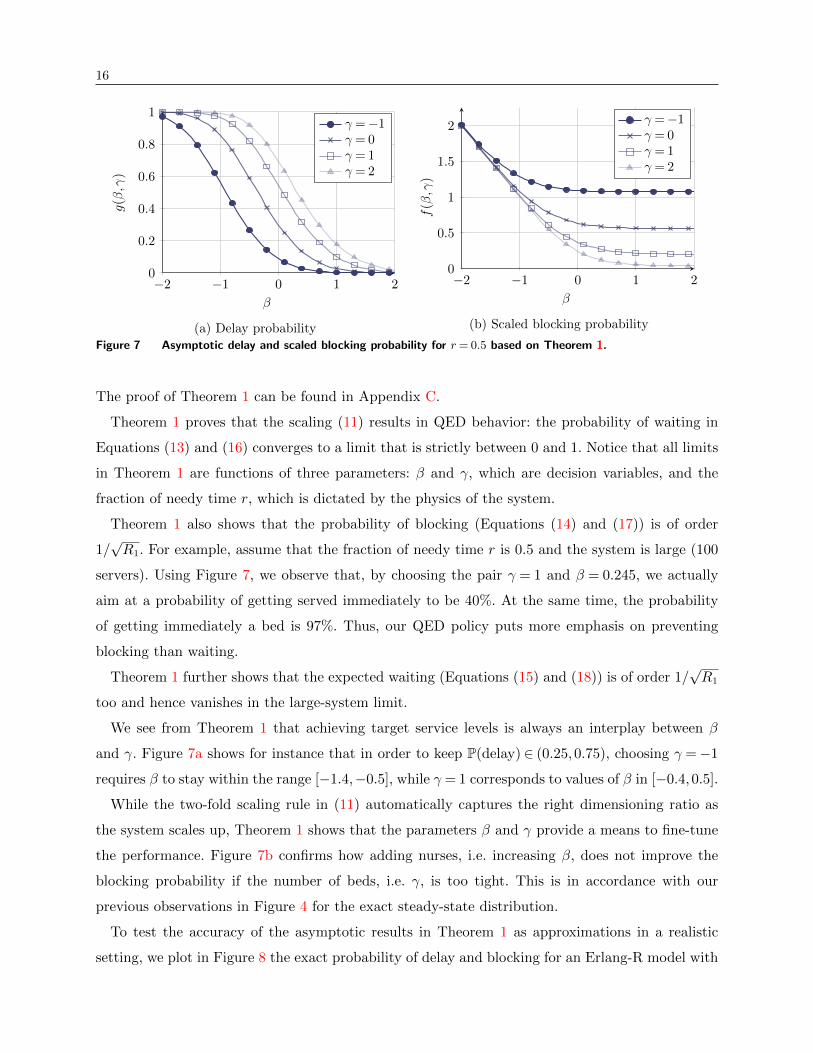
Figure 7 Asymptotic delay and scaled blocking probability for r= 0.5 based on Theorem 1.

The proof of Theorem 1 can be found in Appendix C.

Theorem 1 proves that the scaling (11) results in QED behavior: the probability of waiting in

Equations (13) and (16) converges to a limit that is strictly between 0 and 1. Notice that all limits

in Theorem 1 are functions of three parameters: β and γ, which are decision variables, and the

fraction of needy time r, which is dictated by the physics of the system.

Theorem 1 also shows that the probability of blocking (Equations (14) and (17)) is of order

1/√R1. For example, assume that the fraction of needy time r is 0.5 and the system is large (100

servers). Using Figure 7, we observe that, by choosing the pair γ = 1 and β = 0.245, we actually

aim at a probability of getting served immediately to be 40%. At the same time, the probability

of getting immediately a bed is 97%. Thus, our QED policy puts more emphasis on preventing

blocking than waiting.

Theorem 1 further shows that the expected waiting (Equations (15) and (18)) is of order 1/√R1

too and hence vanishes in the large-system limit.

We see from Theorem 1 that achieving target service levels is always an interplay between β

and γ. Figure 7a shows for instance that in order to keep P(delay) ∈ (0.25,0.75), choosing γ =−1

requires β to stay within the range [−1.4,−0.5], while γ = 1 corresponds to values of β in [−0.4,0.5].

While the two-fold scaling rule in (11) automatically captures the right dimensioning ratio as

the system scales up, Theorem 1 shows that the parameters β and γ provide a means to fine-tune

the performance. Figure 7b confirms how adding nurses, i.e. increasing β, does not improve the

blocking probability if the number of beds, i.e. γ, is too tight. This is in accordance with our

previous observations in Figure 4 for the exact steady-state distribution.

To test the accuracy of the asymptotic results in Theorem 1 as approximations in a realistic

setting, we plot in Figure 8 the exact probability of delay and blocking for an Erlang-R model with

17

0 2 4 6 8 10 12 14 160

0.2

0.4

0.6

0.8

1

s

n= 24n= 28n= 32n= 36n= 40

(a) Delay probability

0 2 4 6 8 10 12 14 160

0.5

1

1.5

2

s

n= 24n= 28n= 32n= 36n= 40

(b) Scaled blocking probabilityFigure 8 Comparison of exact performance restricted (solid) against asymptotic approximations (dashed) with

β = (s−R1)/√R1 and γ = (n−R1/r)/

√R1/r for λ= 2, µ= 1, δ= 0.25 and p= 0.75.

R= 8 and r= 0.25, as a function of s. The exact probabilities are given by Equation (5), and their

respective asymptotic approximations are based on Theorem 1. Despite the realistic moderate size

of the system (R = 8), we see that the QED approximations are remarkably accurate for many

settings (s,n). This fast relaxation is in line with observations made earlier in the QED literature

(Borst et al. 2004, Janssen et al. 2011).

In Appendix E.1, we furthermore compare the asymptotic delay and blocking probability in three

additional scenarios. In Tables EC.2–EC.4 we compute the exact probabilities of delay and blocking

through the explicit forms in (5) for various values of the offered-load R1, which are omitted here

due to space constraints. The numerical results show that gb(β,γ), f b(β,γ) and hb(β,γ) provide

accurate approximations to P(delay),√R1P(block) and

√R1 E[W ] in pre-limit systems. The quality

of the approximations increases with R1. Naturally, fluctuations occur for relatively small values

of R1, because s and n need to be rounded to an integer.

4.3. QED limits for Erlang-R with holding

As explained in §4, the model with holding has no product-form steady-state distribution, which

makes it hard (if not impossible) to obtain QED limits. Instead, we derive QED approximations

by exploiting a connection with the blocking model.

We first prove that under scaling (11), the upper bound on the utilization level of the nurses

needed to achieve stability in the model with holding, as given in Proposition 1, converges to unity

as R→∞. This facilitates high utilization levels of both nurses and beds, a key characteristic of

the QED regime.

Proposition 3. Let s and n scale with R1→∞ as in (11). Then, for λ→∞,

ρmax(s,n)→ 1.

18

The proof can be found in Appendix D. Combining Proposition 3 with Proposition 1 shows that

indeed the scaling we use results in a highly utilized system.

As observed before, the nature of the two variants of the model is similar up to the fact that a

fraction of the patients is deferred on arrive in the setting with blocking, whereas all the arriving

patients are eventually admitted into the system in the holding model. This implies that, given s

and n, the nurses face an increased workload in case of a holding room. In fact, Theorem 1 shows

that the blocking probability is of order 1/√R1, yielding a volume of blocked patients of order

√R1 in setting with blocking. Accordingly, if Rb =R1 and Rh denote the nominal load arriving to

the nurses in the model with blocking and holding, respectively, we can argue that

Rh =Rb +α√Rb + o(

√Rb),

for some α > 0. Notice that this additional load is of the same order as the safety staffing in the

blocking model staffing rule (11). As s and n remain unchanged, we rewrite (11) in terms of Rh,

s=Rh + (β−α)√Rh + o(

√Rh),

n=Rh

r+(γ−α/

√r)√Rh

r+ o(√Rh), (19)

where we have used Rb = O(Rh). Observe that the square-root principle prevails also after this

substitution, albeit with different hedging parameters. We therefore heuristically argue that the

holding model under scaling (11) with parameters β and γ mimics the blocking model with param-

eters β−α and γ−α/√r, respectively.

Observe, however, that we have not yet specified the value of α. By definition, α√Rb is the

expected volume of patients that would be rejected in the model with blocking, that is, Rh times the

probability of not being admitted to the system directly. By the construction in (19), this volume

asymptotically equals Rh ·Pb(block), with parameters β−α and γ−α/√r, which by Theorem 1 is

approximated by

f b(β−α,γ−α/

√r)/√Rh

as Rh grows large. In conclusion, α is characterized as the solution of the fixed-point equation

α= fh(β−α,γ−α/

√r), (20)

and as a result, we are able to approximate the delay probability in the Erlang-R model with

holding as

Ph(delay)≈ gb(β−α,γ−α/√r) =: gh(β,γ). (21)

Likewise, the scaled the mean waiting time for a server can be approximated by√R1 ·E[W ]≈ hb(β−α,γ−α/

√r) =: hh(β,γ). (22)

19

This also implies that the holding queue is O(√R1). Subsequently, we argue that the expected

holding time (pre-entering wait) under the QED policy is O(1/√R1) and hence asymptotically

negligible. We justify this claim numerically in §6.

Remark 2. Notice that in the reasoning leading to (20), we implicitly assumed that the addi-

tional volume α√R1 is an independent Poisson process, which is obviously not the case. Therefore,

(21)–(22) are approximations for pre-limit systems that are not asymptotically correct as λ→∞.

Nevertheless, our heuristic approach seems to performs well as we confirm numerically next.

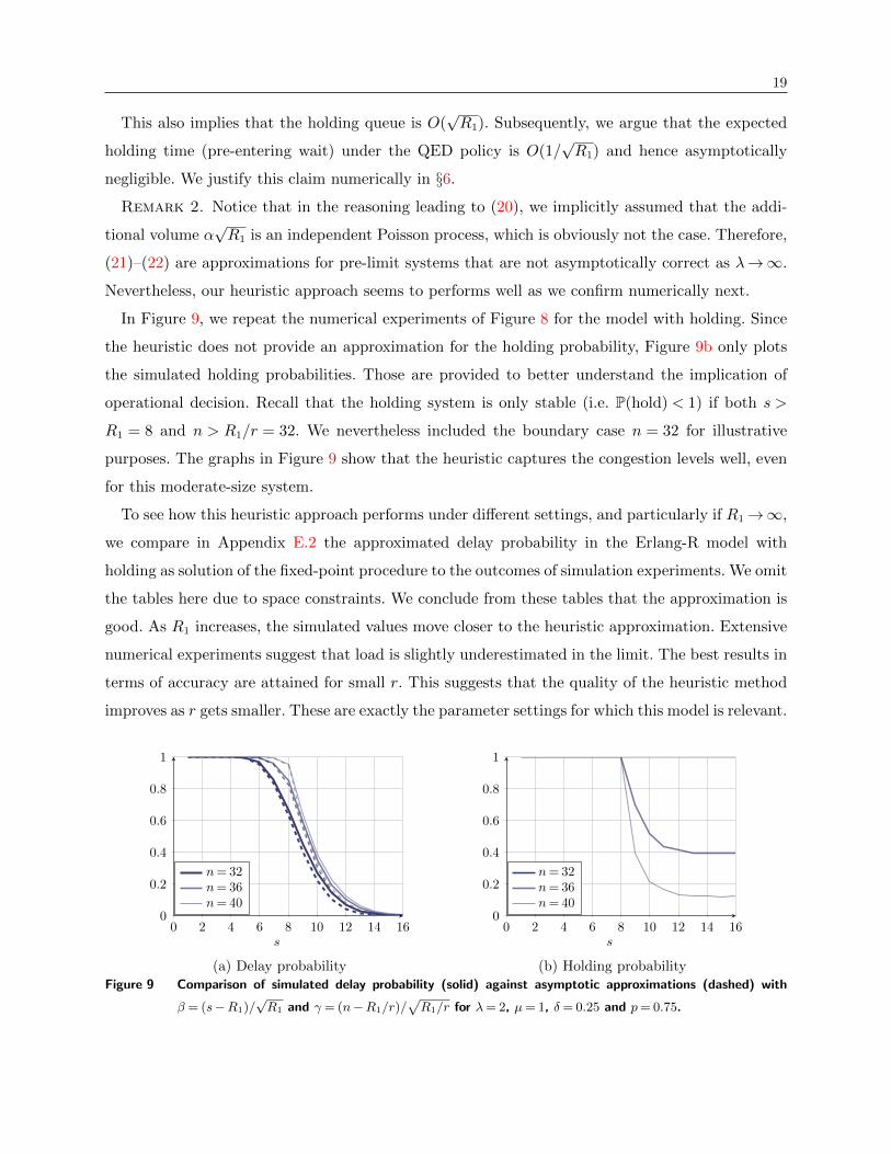
In Figure 9, we repeat the numerical experiments of Figure 8 for the model with holding. Since

the heuristic does not provide an approximation for the holding probability, Figure 9b only plots

the simulated holding probabilities. Those are provided to better understand the implication of

operational decision. Recall that the holding system is only stable (i.e. P(hold) < 1) if both s >

R1 = 8 and n > R1/r = 32. We nevertheless included the boundary case n = 32 for illustrative

purposes. The graphs in Figure 9 show that the heuristic captures the congestion levels well, even

for this moderate-size system.

To see how this heuristic approach performs under different settings, and particularly if R1→∞,

we compare in Appendix E.2 the approximated delay probability in the Erlang-R model with

holding as solution of the fixed-point procedure to the outcomes of simulation experiments. We omit

the tables here due to space constraints. We conclude from these tables that the approximation is

good. As R1 increases, the simulated values move closer to the heuristic approximation. Extensive

numerical experiments suggest that load is slightly underestimated in the limit. The best results in

terms of accuracy are attained for small r. This suggests that the quality of the heuristic method

improves as r gets smaller. These are exactly the parameter settings for which this model is relevant.

0 2 4 6 8 10 12 14 160

0.2

0.4

0.6

0.8

1

s

n= 32n= 36n= 40

(a) Delay probability

0 2 4 6 8 10 12 14 160

0.2

0.4

0.6

0.8

1

s

n= 32n= 36n= 40

(b) Holding probabilityFigure 9 Comparison of simulated delay probability (solid) against asymptotic approximations (dashed) with

β = (s−R1)/√R1 and γ = (n−R1/r)/

√R1/r for λ= 2, µ= 1, δ= 0.25 and p= 0.75.

20

5. Dimensioning

We will now use the accurate asymptotic approximations of the previous section to define a proce-

dure that determines resource capacity in the restricted Erlang-R models. That is, we aim to set

the number of nurses s and the number of beds n, such that a preset performance level is achieved.

We take the probability of delay at the needy queue and the probability of blocking/holding at the

pre-entrant queue as the target performance objectives.

5.1. Capacity setting for Erlang-R with blocking

In the setting with blocking, we can readily use the asymptotic results of Theorem 1 to (numerically)

find a pair of parameters (β∗, γ∗) to meet the performance requirements. For instance, given that

we want the delay probability to be at most ε, we first solve the equation gb(β∗, γ∗) = ε and then

assign s= dR1 +β∗√R1e and n= dR1/r+ γ∗

√R1/re. Note that there could be multiple solutions

to that problem, i.e. there could be multiple combinations of number of beds and number of nurses

that can result in the same value of a single performance level. The system manager can ultimately

decide which of these feasible solutions fits the environment best, for instance taking into account

space and cost constraints.

We illustrate the resource allocation decisions in an MU setting, using data originated from

two articles: Lundgren and Segesten (2001) and Green and Yankovic (2011). Green and Yankovic

describe an MU that has 42 beds, with average occupancy level 78%, and Average Length of Stay

(ALOS) 4.3 days. Lundgren and Segesten studied nurses’ service times in a medical-surgical ward.

They found that the average service time in their unit was 15.3 minutes per service, and that the

average demand rate for each patient is 0.38 requests per hour. Therefore, we take an average

service time of 15 minutes and assume that there are 0.4 requests per hour from each patient.

Fitting this data to our model results in the following parameters values: λ= 0.32, µ= 4, δ = 0.4,

p= 0.975 and the fraction of needy time is then approximately r= 0.09. This yields nominal offered

load R1 = 3.2 and R1/r= 34.4.

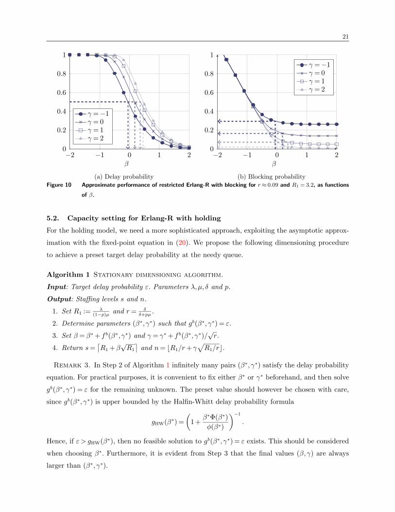
Figure 10 visualizes the dimensioning procedure for this particular MU. The hospital manage-

ment can find a pair of n and s to meet certain criteria, for example to achieve target delay

probability ε= 0.5 with reasonable blocking probability. Figure 10a indicates that this target can

be achieved by a variety of pairs, for instance (β1, γ1) = (−0.06,−1), (β2, γ2) = (0.16,0), (β3, γ3) =

(0.36,1) or (β4, γ4) = (0.46,2), among infinitely many others. According to Figure 10b, the pairs

named above lead to blocking probabilities 0.293, 0.165, 0.071 and 0.021, respectively. If the man-

ager decides that probability of blocking of more than 10 percent is not acceptable, this leaves the

choices (β3, γ3) = (0.36,1) or (β4, γ4) = (0.46,2) as candidate parameter pairs. Using the two-fold

square-root staffing rule si = dR1 +βi√R1e and ni = [R1/r+ γ

√R1/r], this yields feasible staffing

levels (s3, n3) = (4,40) and (s4, n4) = (5,46). The ultimate decision to apply any of these solutions

can be based on external factors, such as operational costs or space limitations of number of beds.

21

−2 −1 0 1 20

0.2

0.4

0.6

0.8

1

β

γ =−1γ = 0γ = 1γ = 2

(a) Delay probability

−2 −1 0 1 20

0.2

0.4

0.6

0.8

1

β

γ =−1γ = 0γ = 1γ = 2

(b) Blocking probabilityFigure 10 Approximate performance of restricted Erlang-R with blocking for r≈ 0.09 and R1 = 3.2, as functions

of β.

5.2. Capacity setting for Erlang-R with holding

For the holding model, we need a more sophisticated approach, exploiting the asymptotic approx-

imation with the fixed-point equation in (20). We propose the following dimensioning procedure

to achieve a preset target delay probability at the needy queue.

Algorithm 1 Stationary dimensioning algorithm.

Input: Target delay probability ε. Parameters λ,µ, δ and p.

Output: Staffing levels s and n.

1. Set R1 := λ(1−p)µ and r= δ

δ+pµ.

2. Determine parameters (β∗, γ∗) such that gb(β∗, γ∗) = ε.

3. Set β = β∗+ f b(β∗, γ∗) and γ = γ∗+ f b(β∗, γ∗)/√r.

4. Return s=⌈R1 +β

√R1

⌉and n= bR1/r+ γ

√R1/rc.

Remark 3. In Step 2 of Algorithm 1 infinitely many pairs (β∗, γ∗) satisfy the delay probability

equation. For practical purposes, it is convenient to fix either β∗ or γ∗ beforehand, and then solve

gb(β∗, γ∗) = ε for the remaining unknown. The preset value should however be chosen with care,

since gb(β∗, γ∗) is upper bounded by the Halfin-Whitt delay probability formula

gHW(β∗) =

(1 +

β∗Φ(β∗)

φ(β∗)

)−1

.

Hence, if ε > gHW(β∗), then no feasible solution to gb(β∗, γ∗) = ε exists. This should be considered

when choosing β∗. Furthermore, it is evident from Step 3 that the final values (β,γ) are always

larger than (β∗, γ∗).

22

We now use the same example as in §5.1 to demonstrate capacity allocation decisions for the

model with holding. This can be viewed as the additional capacity the MU needs in terms of nurses

and beds, in order to account for the fact that patients are waiting in the ED to be admitted,

into the preferred MU, instead of being blocked and transferred to a less preferred unit. Observe

that the holding model leaves less flexibility for management in choosing system parameters due

to stability constraints. For example, the policy with n= 30 (γ =−0.75) is infeasible in the holding

model. For similar reasons, only nurse staffing levels with β > 0, or s >R1 = 3.2 are feasible.

Targeting a delay probability of 0.5 with n= 40, Figure 11 shows that operating an MU with

holding room requires β = 0.475 or s= 5. Recall that under the blocking policy, only s= 4 nurses

were needed to achieve a delay probability of 0.5. This example hence shows how the managerial

decision to have a holding room, rather than deferring patients to less preferred medical units,

requires additional workforce in that unit (as well as the ED). This example also shows that

the facility with holding room is able to treat fewer patients simultaneously than under blocking

constraints, in line with the bounds in §3.3 and Conjecture 1.

0 0.5 1 1.5 20

0.2

0.4

0.6

0.8

1

β

gh(β,γ

)

γ =−0.75γ = 0.102γ = 0.955

Figure 11 Approximate delay probability of restricted Erlang-R system with holding for r≈ 0.09 and R1 = 3.2

6. Model analysis and managerial implications

In this section, we use the analysis and algorithms developed in earlier sections to gain insights into

the importance of the capacity restrictions and customer returns in a restricted Erlang-R system

by drawing a comparison to related models studied in the literature.

23

0 0.2 0.4 0.6 0.8 10

0.2

0.4

0.6

0.8

r

β = 0.25β = 0.5β = 1.0β = 2.0

(a) Delay probability

0 0.2 0.4 0.6 0.8 10

0.1

0.2

0.3

0.4

r

β = 0.25β = 0.5β = 1.0β = 2.0

(b) Scaled blocking probabilityFigure 12 Asymptotic performance measures as a function of r in the restricted Erlang-R model with blocking

for γ = 1.

6.1. The influence of customer returns or the role of r

Here we study how the parameter r affects the service level in the restricted Erlang-R model with

blocking, on the basis of the asymptotic expressions in Theorem 1.

To better understand the connection with the single-station model and the importance of returns

we examine the role of r. Recall the interpretation of r as the fraction of time a patient is needy

during his stay within the system in the idealized scenario with infinite capacity, i.e. for r ∈ (0,1).

The case r = 1 corresponds to the setting in which patients are needy all the time, in this case

customers get service in one time. When r = 1 the infinite-server queue, describing the number

of content patients, disappears from the queueing system and we end up with a standard loss

model—M/M/s/n queue—in which capacity is scaled as

s=R1 +β√R1, n=R1 + γ

√R1.

This staffing rule only makes sense in case β < γ, since no delay is experienced if n≤ s. If indeed

γ > β, then the asymptotic delay probability and scaled blocking probability are given by Massey

and Wallace (2004),

gB(β,γ) =1− e−β(γ−β)

1− e−β(γ−β) +βΦ(β)/φ(β), fB(β,γ) =

βe−β(γ−β)

1− e−β(γ−β) +βΦ(β)/φ(β).

We can see that f b(β,γ) of increasing β approaches a lower bound that is a function of r. To

see this, observe that as β grows, delays at the nurse queue vanish. Then the sojourn time of an

admitted patient only consists of a geometric number of needy and content periods with mean

(1/µ+p/δ)/(1−p) = 1/rµ(1−p). The blocking model can in this case be modeled as an M/G/n/n

24

queue, with offered load λ/(rµ(1− p)) =R1/r, in which the scaled blocking probability is known

to be, see Janssen et al. (2008),√R1 P(block) =

√R1

(R1/r)n/n!∑n

k=0(R1/r)k/k!→√rφ(γ)

Φ(γ),

as R1→∞. This function of r is plotted in Figure 12b as the dashed line.

We observe that in general the probability of blocking increases with r, regardless of the capacity

constraints on the needy station. We can explain this by observing that r influences only n in

the QED staffing rule. When n reduces, more patients are blocked. Therefore, if customers spend

relatively more time in needy state, which usually indicates services that are less interrupted,

blocking will increase. Delays, on the other hand, will decrease in such situations—the minimal

delay possible can be achieved if service is given in one time (r = 1). Returns or interruptions

increase delays significantly under QED staffing.

Managerial insight 3

1. Returning customers should be explicitly accounted for in determining staffing in a system

with space constraints both in steady-state and transient conditions.

2. The above becomes more important as the proportion of time spend in needy state becomes

small, since then the number of customer contributing to the space constrains increases.

3. As returns become more spread over the patient’s length-of-stay (r decreases), delay increases

and blocking decreases.

6.2. Comparing restricted and unrestricted Erlang-R models

Given the expressions for the asymptotic delay probability in the open Erlang-R model, and its

restricted versions with blocking and holding, we compare the three policies for various values of

β, γ and r. Figure 13 plots the delay probability for blocking (gb(β,γ)), holding (gh(β,γ)) and

Erlang-R (gHW(β)) models, as functions of γ, while keeping β fixed, for three values of r. We make

a couple of observations. Notice that

gb(β,γ)≤ gh(β,γ)≤ gHW(β)

for all β,γ > 0 and r. In that sense, the holding model is an interpolation between the blocking and

the open model. As expected, the delay probabilities in the restricted models converge to those of

the open Erlang-R model, because increasing γ is tantamount to lifting the stringent constraints

on the system size. Note that the rate of conversion is fast—one can provide probability of waiting

close to that of the open model with small values of γ. Indeed, the fact that when using QED

staffing not much of excessive delay results from the beds restriction is important by itself. Also,

we observe that the difference between delay probabilities increases with r.

25

0 0.5 1 1.5 2 2.5 30

0.2

0.4

0.6

0.8

1

→ γ

β = 0.1 β = 0.5 β = 1

(a) r= 0.1.

0 0.5 1 1.5 2 2.5 30

0.2

0.4

0.6

0.8

1

→ γ

β = 0.1 β = 0.5 β = 1

(b) r= 0.25.

0 0.5 1 1.5 2 2.5 30

0.2

0.4

0.6

0.8

1

→ γ

β = 0.1 β = 0.5 β = 1

(c) r= 0.5.Figure 13 Asymptotic delay probability in open Erlang-R (dashed), restricted Erlang-R with blocking (•) and

restricted Erlang-R with holding (�), as function of γ.

6.3. The impact of visit number

We next reflect on the impact of operational capacity decisions on different customer populations.

We measure patient’s complexity by the number of times she needs to see the nurse or the physician

during her stay. In the ED context, simple-to-treat patients will need to see the physician once,

while complex ones will need multiple visits. Hence, we divide the patients into complexity groups

by the number of visits in the needy station. Since the number of visits is geometrically distributed,

we have a higher proportion of simple patients than complex ones; that fits well the health care

environment.

Figure 14 shows the waiting time in the needy and pre-entring queues, and the total waiting

time, as a function n (number of beds), for each complexity group. Obviously, the expected waiting

time in the pre-entring queue decreases with n, while the needy waiting time increases. For patients

who require a relative large number of visits of the physician, in this case more than 6, the total

needy wait is the dominant part of the total waiting time. Therefore, as n grows, the total waiting

time first decreases and then increases. In fact, Figure 14b suggests that there is an optimal number

of beds n that minimizes the total wait for each complexity type. Thus, size restrictions reduce

the length-of-stay of patients with complex health conditions (given that the constraint is not

too tight). On the other hand, this figure also shows that no such n exists for patients who only

require little assistance. Hence, there is no n that improves the sojourn time of all patients in the

ED simultaneously. This leaves the decision to the hospital manager to weigh the importance of

patients of different complexity levels.

Remark 4. From a different perspective, note that in communication queueing systems, the

partition of a job to sizable quantities and scheduling those jobs in a similar dynamic to the Erlang-

R model became a popular way for increasing throughput. This is because this effectively schedule

jobs by their size even though the total job requirements are uncertain. This in fact creates a

26

shortest-job-first policy without prior knowledge of job size (Bonald and Comte 2016). Considering

that perspective we note that the Erlang-R model actually prioritize simple jobs over complex

ones. But without restrictions, when load is too high, such procedures may lead to very long LOS

of long jobs. The capacity restriction we analyze in this paper, in both of its versions, limits such

delays. Hence, even in cases in which the returns themselves are created by a managerial decision,

imposing the additional managerial restriction on entering the system has benefits.

35 40 45 50 55 600

2

4

6

8

10

n

(a) Expected pre-entering waiting (•)

and needy waiting times (�)

35 40 45 50 55 600

2

4

6

8

10

n

N = 1N = 2N = 3N = 4N = 5N = 6N = 7N = 8N = 9N = 10

(b) Total expected

waiting timesFigure 14 Expected waiting times as a function of n given the number of visits N in the Erlang-R model with

holding with λ= 2 µ= 1, δ= 0.25, p= 0.75 and s= 9.

6.4. Case study: comparison of operational decisions

We now illustrate how the managerial decision to operate under a specific operational regime affects

ED performance in terms of efficiency and quality-of-care, through a case study. The practical

environment we investigate is the ED of a moderately-sized hospital, which faces the arrival pattern

λ(t) plotted in Figure 15a on a typical workday. Other parameters of the model are estimated to

be µ= 6.67, δ = 2.18 and p= 0.76, so that r = 0.301. (Parameters were taken from Yom-Tov and

Mandelbaum (2014)). In order to set time-varying staffing levels s(t) and n(t), we adopt the MOL

approximation of the demand process of Jennings et al. (1996). This approach initially presumes

infinite capacity to obtain the number of customers R(t) in the queueing system as a function of

time. This offered load function then replaces (constant) value of R in the stationary dimensioning

scheme under consideration, to determine the adequate number of servers at each point in time.

Following this idea in our two-dimensional queueing system, we find the offered load function for

the nurses R1(t) and the offered load function for the beds R1(t) +R2(t) as the solution of the

system of ODEs,

d

dtR1(t) = λ(t) + δR2(t)−µR1(t), (23)

27

0 5 10 15 200

10

20

30

40

→ t

λ(t)

R1(t)

R1(t) +R2(t)

(a) Dynamic arrival rate and load functions

0 5 10 15 200

10

20

30

40

→ t

s(t)

n(t)

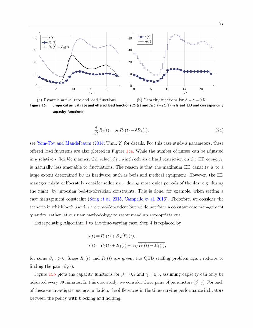
(b) Capacity functions for β = γ = 0.5Figure 15 Empirical arrival rate and offered load functions R1(t) and R1(t)+R2(t) in Israeli ED and corresponding

capacity functions

d

dtR2(t) = pµR1(t)− δR2(t), (24)

see Yom-Tov and Mandelbaum (2014, Thm. 2) for details. For this case study’s parameters, these

offered load functions are also plotted in Figure 15a. While the number of nurses can be adjusted

in a relatively flexible manner, the value of n, which echoes a hard restriction on the ED capacity,

is naturally less amenable to fluctuations. The reason is that the maximum ED capacity is to a

large extent determined by its hardware, such as beds and medical equipment. However, the ED

manager might deliberately consider reducing n during more quiet periods of the day, e.g. during

the night, by imposing bed-to-physician constraints. This is done, for example, when setting a

case management constraint (Song et al. 2015, Campello et al. 2016). Therefore, we consider the

scenario in which both s and n are time-dependent but we do not force a constant case management

quantity, rather let our new methodology to recommend an appropriate one.

Extrapolating Algorithm 1 to the time-varying case, Step 4 is replaced by

s(t) =R1(t) +β√R1(t),

n(t) =R1(t) +R2(t) + γ√R1(t) +R2(t),

for some β,γ > 0. Since R1(t) and R2(t) are given, the QED staffing problem again reduces to

finding the pair (β,γ).

Figure 15b plots the capacity functions for β = 0.5 and γ = 0.5, assuming capacity can only be

adjusted every 30 minutes. In this case study, we consider three pairs of parameters (β,γ). For each

of these we investigate, using simulation, the differences in the time-varying performance indicators

between the policy with blocking and holding.

28

0 3 6 9 12 15 18 21 240

0.2

0.4

0.6

0.8

1

→ t

(a) P(delay)

0 3 6 9 12 15 18 21 240

0.1

0.2

0.3

0.4

0.5

→ t

(β,γ) = (0.1,2)

(β,γ) = (1,1.5)

(β,γ) = (2,1)

(b) P(block) or P(hold)

0 3 6 9 12 15 18 21 240

1

2

3

4

5

→ t

(c) Nurse-to-patient ratio.

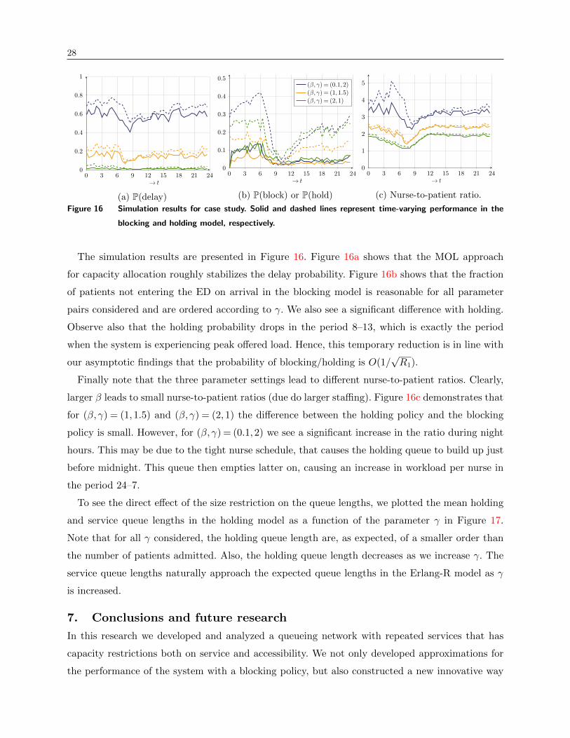
Figure 16 Simulation results for case study. Solid and dashed lines represent time-varying performance in the

blocking and holding model, respectively.

The simulation results are presented in Figure 16. Figure 16a shows that the MOL approach

for capacity allocation roughly stabilizes the delay probability. Figure 16b shows that the fraction

of patients not entering the ED on arrival in the blocking model is reasonable for all parameter

pairs considered and are ordered according to γ. We also see a significant difference with holding.

Observe also that the holding probability drops in the period 8–13, which is exactly the period

when the system is experiencing peak offered load. Hence, this temporary reduction is in line with

our asymptotic findings that the probability of blocking/holding is O(1/√R1).

Finally note that the three parameter settings lead to different nurse-to-patient ratios. Clearly,

larger β leads to small nurse-to-patient ratios (due do larger staffing). Figure 16c demonstrates that

for (β,γ) = (1,1.5) and (β,γ) = (2,1) the difference between the holding policy and the blocking

policy is small. However, for (β,γ) = (0.1,2) we see a significant increase in the ratio during night

hours. This may be due to the tight nurse schedule, that causes the holding queue to build up just

before midnight. This queue then empties latter on, causing an increase in workload per nurse in

the period 24–7.

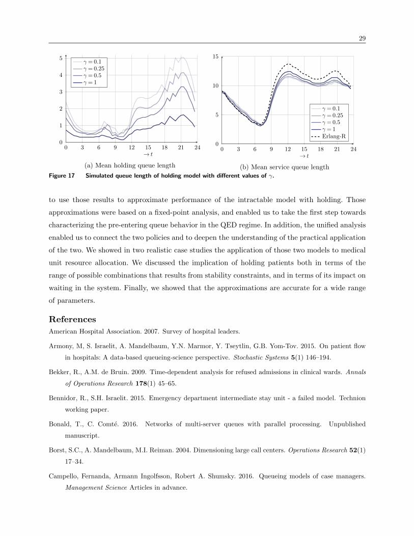
To see the direct effect of the size restriction on the queue lengths, we plotted the mean holding

and service queue lengths in the holding model as a function of the parameter γ in Figure 17.

Note that for all γ considered, the holding queue length are, as expected, of a smaller order than

the number of patients admitted. Also, the holding queue length decreases as we increase γ. The

service queue lengths naturally approach the expected queue lengths in the Erlang-R model as γ

is increased.

7. Conclusions and future research

In this research we developed and analyzed a queueing network with repeated services that has

capacity restrictions both on service and accessibility. We not only developed approximations for

the performance of the system with a blocking policy, but also constructed a new innovative way

29

0 3 6 9 12 15 18 21 240

1

2

3

4

5

→ t

γ = 0.1γ = 0.25γ = 0.5γ = 1

(a) Mean holding queue length

0 3 6 9 12 15 18 21 240

5

10

15

→ t

γ = 0.1γ = 0.25γ = 0.5γ = 1Erlang-R

(b) Mean service queue lengthFigure 17 Simulated queue length of holding model with different values of γ.

to use those results to approximate performance of the intractable model with holding. Those

approximations were based on a fixed-point analysis, and enabled us to take the first step towards

characterizing the pre-entering queue behavior in the QED regime. In addition, the unified analysis

enabled us to connect the two policies and to deepen the understanding of the practical application

of the two. We showed in two realistic case studies the application of those two models to medical

unit resource allocation. We discussed the implication of holding patients both in terms of the

range of possible combinations that results from stability constraints, and in terms of its impact on

waiting in the system. Finally, we showed that the approximations are accurate for a wide range

of parameters.

References

American Hospital Association. 2007. Survey of hospital leaders.

Armony, M, S. Israelit, A. Mandelbaum, Y.N. Marmor, Y. Tseytlin, G.B. Yom-Tov. 2015. On patient flow

in hospitals: A data-based queueing-science perspective. Stochastic Systems 5(1) 146–194.

Bekker, R., A.M. de Bruin. 2009. Time-dependent analysis for refused admissions in clinical wards. Annals

of Operations Research 178(1) 45–65.

Bennidor, R., S.H. Israelit. 2015. Emergency department intermediate stay unit - a failed model. Technion

working paper.

Bonald, T., C. Comte. 2016. Networks of multi-server queues with parallel processing. Unpublished

manuscript.

Borst, S.C., A. Mandelbaum, M.I. Reiman. 2004. Dimensioning large call centers. Operations Research 52(1)

17–34.

Campello, Fernanda, Armann Ingolfsson, Robert A. Shumsky. 2016. Queueing models of case managers.

Management Science Articles in advance.

30

Carmen, R., I. van Nieuwenhuyse. 2016. How inpatient boarding impacts ED performance: A queueing

analysis. Working paper, KU Leuven.

Chen, H., D.D. Yao. 2001. Fundamentals of Queueing Networks: Performance, Asymptotics, and Optimiza-

tion. Springer.

de Bruin, A.M., R. Bekker, L. van Zanten, G.M. Koole. 2009. Dimensioning hospital wards using the Erlang

loss model. Annals of Operations Research 178(1) 23–43.

Denton, B.T., ed. 2013. Handbook of healthcare operations management: Methods and applications. 2nd ed.

North Holland, New York.

Diwas, KC S. 2014. Does multitasking improve performance? evidence from the emergency department.

Manufacturing & Service Operations Management 16(2) 168–183.

Gamarnik, D., D.A. Goldberg. 2013. On the rate of convergence to stationarity of the M/M/N queue in the

Halfin-Whitt regime. The Annals of Applied Probability 23(5) 1879–1912.

Green, L., N. Yankovic. 2011. Identifying good nursing levels: A queuing approach. Operations Research

59(4) 942–955.

Green, L.V. 2006. Using queueing theory to increase the effectiveness of physician staffing in the emergency

department. Academic Emergency Medicine 13 61–68.

Green, L.V., S. Savin. 2008. Reducing delays for medical appointments: A queueing approach. Operations

Research 56(6) 1526–1538.

Halfin, S., W. Whitt. 1981. Heavy-traffic limits for queues with many exponential servers. Operations

Research 29(3) 567–588.

Hall, R.W., ed. 2006. Patient Flow: Reducing Delay in Healthcare Delivery . Springer.

Hall, R.W., ed. 2012. Handbook of Healthcare System Scheduling . Springer.

Huang, Junfei, Boaz Carmeli, Avishai Mandelbaum. 2015. Control of patient flow in emergency departments,

or multiclass queues with deadlines and feedback. Operations Research 63(4) 892–908.

Jackson, J.R. 1963. Jobshop-like queueing systems. Management Science 10(1) 131–142.

Janssen, A.J.E.M., J.S.H. van Leeuwaarden, B. Zwart. 2008. Gaussian expansions and bounds for the Poisson

distribution applied to the Erlang-B formula. Advances in Applied Probability 40(1) 122–143.

Janssen, A.J.E.M., J.S.H. van Leeuwaarden, B. Zwart. 2011. Refining square-root safety staffing by expanding

erlang c. Operations Research 59(6) 1512–1522.

Jennings, O.B., F. de Vericourt. 2008. Dimensioning large-scale memberschip services. Operations Research

55(1) 173–187.

Jennings, O.B., F. de Vericourt. 2011. Nurse staffing in medical units: A queueing perspective. Operations

Research 59(6) 1320–1331.

31

Jennings, O.B., A. Mandelbaum, W.A. Massey, W. Whitt. 1996. Server staffing to meet time-varying demand.

Management Science 42(10) 1383–1394.

Kazahaya, G. 2005. Harnessing technology to redesign labor cost management reports. Healthcare Financial

Management 59(4) 94–100.

Khudyakov, P., P.D. Feigin, A. Mandelbaum. 2010. Designing a call center with an IVR (Interactive Voice

Response). Queueing Systems 66(3) 215–237.

Lundgren, S., K. Segesten. 2001. Nurses use of time in a medical-surgical ward with all-rn staffing. Journal

of Nursing Management 9(1) 13–20.

Massey, W.A., R.B. Wallace. 2004. An asymptotically optimal design of the M/M/c/k queue. Unpublished

report.

Neuts, M.F. 1981. Matrix-Geometric Solutions in Stochastic Models. The John Hopkins University Press,

Baltimore.

Sanders, J., S.C. Borst, A.J.E.M. Janssen, J.S.H. vvan Leeuwaarden. 2016. Optimality gaps in asymptotic

dimensioning of many-server systems. Operations Research Letters 44(3) 369–365.

Song, Hummy, Anita L. Tucker, Karen L. Murrell. 2015. The diseconomies of queue pooling: An empirical

investigation of emergency department length of stay. Management Science 61(12) 3032–3053.

van Leeuwaarden, J.S.H., C. Knessl. 2011. Transient behavior of the halfinwhitt diffusion. Stochastic Pro-

cesses and their Applications 1524–1545.

van Leeuwaarden, J.S.H., C. Knessl. 2012. Spectral gap of the Erlang-A model in the Halfin-Whitt regime.

Stochastic Systems 2(1) 149–207.

van Leeuwaarden, J.S.H., B.W.J. Mathijsen, F. Sloothaak. 2015. Delayed workload shifting in many-server

systems. ACM SIGMETRICS Performance Evaluation Review 43(2) 10–12.

van Leeuwaarden, J.S.H., B.W.J. Mathijsen, F. Sloothaak. 2016. Cloud provisioning in the QED regime.

Proceedings of the 9th EAI International Conference on Performance Evaluation Methodologies and

Tools 180–187.

Yom-Tov, G.B, A. Mandelbaum. 2014. Erlang-R: A time-varying queue with reentrant customers, in support

of healthcare staffing. Manufacturing & Service Operations Management 16(2) 283–299.

Zhang, B., J.S.H. van Leeuwaarden, B. Zwart. 2012. Refining square-root staffing for call centers with

impatient customers. Operations Research 60 461–474.

Zychlinski, N., A. Mandelbaum, P. Momcilovic, I. Cohen. 2016. Bed blocking in hospitals due to scarce

capacity in geriatric institutions – cost minimization via fluid models. Under review.

ec1

Appendix A: Description of the QBD process

A.1. The QBD-process

We consider the QBD-processX = {N,Q1} in stationarity. Let ν(i) = min{i, s}µ. To determine the (outgoing)

transition rates of the process X we distinguish between the following cases:

• Transitions from (0,0): There are no patients in the Emergency Department and thus the only possible

occurrence is when a new patient arrives. This results in a transition to (1,1) and occurs with rate λ.

• Transitions from (i,0),1≤ i < n: There are exactly i patients assigned to a bed of which none are seen

by a nurse. Then either one of those patients becomes needy, or a new patient arrives at the Emergency

Department that can immediately be seen by a nurse. The first results in a transition to (i,1) and

occurs at rate iδ, and the second results in a transition to (i+ 1,1) and occurs with rate λ.

• Transitions from (i,0), i ≥ n: Again, the only possible transitions arises from either a newly arrived

patient or a patient assigned to a bed becoming needy. However, a newly arrived patient finds all beds

occupied and needs to wait. Thus, with rate λ we have a transition to (i+ 1,0) and with rate nδ a

transition to (i,1).

• Transitions from (i, i), i < n: In this case all patients assigned to a bed are in need of service. With rate

λ a new patient arrives at the Emergency Department. She joins the (possible) queue to be seen by a

nurse immediately, so this results in a transition to (i+ 1, i+ 1). Moreover, since there are only s < n

nurses, a service completion occurs with rate ν(i). With probability p the patient turns to the holding

phase, so in total we still have i patients with one patient less in queue for a nurse. With probability

1−p the patient leaves the Emergency Department, decreasing both N and Q1 by one. In other words,

with rate pν(i) we have a transition to (i, i − 1) and with rate (1 − p)ν(i) we have a transition to

(i− 1, i− 1).

• Transitions from (n,n): Similar to the previous case, we have a transition to (n,n− 1) with rate psµ

and with rate (1− p)sµ we have a transition to (n− 1, n− 1). In this case however, a newly arrived

patient finds all beds occupied, resulting in a transition to (n+ 1, n) with rate λ.

• Transitions from (i, n), i > n: We have a transition to (i+ 1, n) with rate λ and a transition to (i, n−1)

with rate psµ. In case that a patient leaves the Emergency Department there are i−n> 0 patients in

the holding room waiting for an available bed. Thus, one of the i− n patients in the holding room is

assigned to the available bed in need of service. That is, with rate (1− p)sµ we have a transition to

(i− 1, n).

• Transitions from (i, j),1≤ j < i < n: There are four possible transitions. First, with rate λ there is a

new arrival which results in a transition to (i+ 1, j + 1). Second, with rate (i− j)δ a patient in one

of the beds becomes needy, which results in a transition to (i, j + 1). Third, with rate pν(j) a patient

turns to the content state after service completion, which results in a transition to (i, j−1). Last, with

rate (1− p)ν(j) a patient leaves the Emergency Department after service completion, which results in

a transition to (i− 1, j− 1).

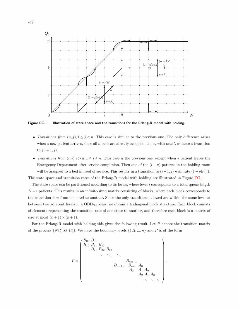
ec2

0

j

k

n

i n

Q1

N

λ(1− p)ν(k)(n− k)δ

pν(k)

λ

(1− p)ν(j)

(i− j)δ

pν(j)

Figure EC.1 Illustration of state space and the transitions for the Erlang-R model with holding.

• Transitions from (n, j),1≤ j < n: This case is similar to the previous one. The only difference arises

when a new patient arrives, since all n beds are already occupied. Thus, with rate λ we have a transition

to (n+ 1, j).

• Transitions from (i, j), i > n,1≤ j ≤ n: This case is the previous one, except when a patient leaves the

Emergency Department after service completion. Then one of the (i−n) patients in the holding room

will be assigned to a bed in need of service. This results in a transition to (i−1, j) with rate (1−p)ν(j).

The state space and transition rates of the Erlang-R model with holding are illustrated in Figure EC.1.

The state space can be partitioned according to its levels, where level i corresponds to a total queue length

N = i patients. This results in an infinite-sized matrix consisting of blocks, where each block corresponds to

the transition flow from one level to another. Since the only transitions allowed are within the same level or

between two adjacent levels in a QBD-process, we obtain a tridiagonal block structure. Each block consists

of elements representing the transition rate of one state to another, and therefore each block is a matrix of

size at most (n+ 1)× (n+ 1).

For the Erlang-R model with holding this gives the following result. Let P denote the transition matrix

of the process {N(t),Q1(t)}. We have the boundary levels {1,2, ..., n} and P is of the form

P =

B00 B01

B10 B11 B12

B21 B22 B23

. . .. . .

. . .

Bnn−1

Bn−1n Bnn A0

A2 A1 A0

A2 A1 A0

. . .. . .

. . .

,

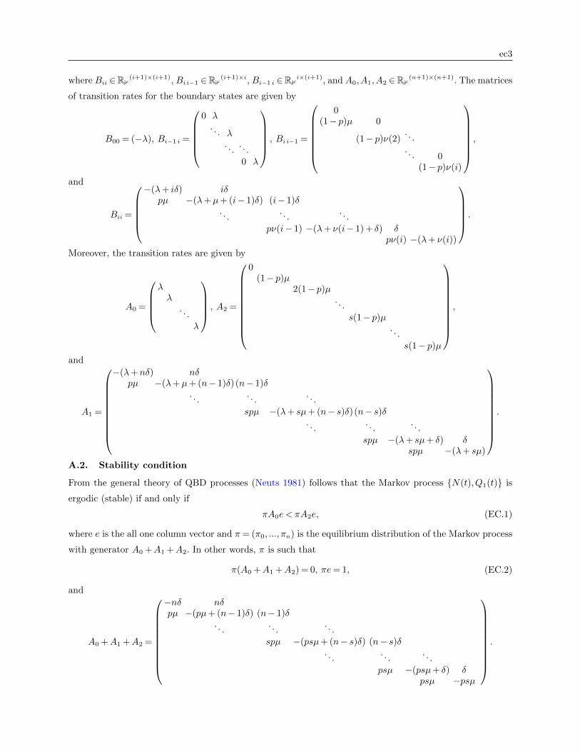
ec3

where Bii ∈R1(i+1)×(i+1), Bi i−1 ∈R1

(i+1)×i, Bi−1 i ∈R1i×(i+1), and A0,A1,A2 ∈R1

(n+1)×(n+1). The matrices

of transition rates for the boundary states are given by

B00 = (−λ), Bi−1 i =

0 λ

. . . λ. . .

. . .

0 λ

, Bi i−1 =

0

(1− p)µ 0

(1− p)ν(2). . .

. . . 0(1− p)ν(i)

,

and

Bii =

−(λ+ iδ) iδ

pµ −(λ+µ+ (i− 1)δ) (i− 1)δ. . .

. . .. . .

pν(i− 1) −(λ+ ν(i− 1) + δ) δpν(i) −(λ+ ν(i))

.

Moreover, the transition rates are given by

A0 =

λλ

. . .

λ

, A2 =

0(1− p)µ

2(1− p)µ. . .

s(1− p)µ. . .

s(1− p)µ

,

and

A1 =

−(λ+nδ) nδpµ −(λ+µ+ (n− 1)δ)(n− 1)δ

. . .. . .

. . .

spµ −(λ+ sµ+ (n− s)δ)(n− s)δ. . .

. . .. . .

spµ −(λ+ sµ+ δ) δspµ −(λ+ sµ)

.

A.2. Stability condition

From the general theory of QBD processes (Neuts 1981) follows that the Markov process {N(t),Q1(t)} is

ergodic (stable) if and only if

πA0e < πA2e, (EC.1)

where e is the all one column vector and π= (π0, ..., πn) is the equilibrium distribution of the Markov process

with generator A0 +A1 +A2. In other words, π is such that

π(A0 +A1 +A2) = 0, πe= 1, (EC.2)

and

A0 +A1 +A2 =

−nδ nδpµ −(pµ+ (n− 1)δ) (n− 1)δ

. . .. . .

. . .

spµ −(psµ+ (n− s)δ) (n− s)δ. . .

. . .. . .

psµ −(psµ+ δ) δpsµ −psµ

.

ec4

Then π must satisfy the balance equations

−nδπ0 + pµπ1 = 0,

(n− j+ 1)δπj−1− (pν(j) + (n− j)δ)πj + pν(j+ 1)πj+1 = 0,

δπn−1− psµπn = 0,

with ν(j) = min{j, s}µ, and the normalization conditionn∑i=0

πi = 1.

It is readily verified that

πi =

π0

(n

i

)(δpµ

)ifor 0≤ i≤ s,

π0

(n

i

)i!s!ss−i

(δpµ

)ifor s+ 1≤ i≤ n

(EC.3)

with

π0 =

(s∑i=0

(n

i

)(δ

pµ

)i+

n∑i=s+1

(n

i

)i!

s!ss−i

(δ

pµ

)i)−1

.

satisfies the balance equations and the normalization condition.

Proposition EC.1. The distribution of the closed two-node Jackson network illustrated in Figure 2a is

given by

πi =

π0

(n

i

)(δpµ

)ifor 0≤ i≤ s,

π0

(n

i

)i!s!ss−i

(δpµ

)ifor s+ 1≤ i≤ n

(EC.4)

with

π0 =

[s∑i=0

(n

i

)(δ

pµ

)i+

n∑i=s+1

(n

i

)i!

s!ss−i

(δ

pµ

)i]−1

.

W e have a two-node closed Jackson network, with probability transition matrix

P =

(1− p p

1 0

).

Let ri(m) denote the rate of service when there are m patient at queue i, so r1(m) = min{m,s} and r2(m) =

m. The throughput vector γ = (γ1, γ2) ∈R12 must satisfy γ = γP and we find that γ = (p,1) suffices. From

the general theory of Jackson networks, see Jackson (1963), it follows that the stationary distribution is

given by

πi =G−1g1(i)g2(n− i)

with

g1(i) = (γ1/µ)i∏im=1 r1(m)

, g2(n− i) = (γ2/δ)n−i∏n−i

m=1 r2(m),

and normalization constant G=∑n

i=0 g1(i)g2(n− i). Then,

g1(i) =

{ 1i!µi

for 0≤ i≤ s,1

s!si−sµifor s+ 1≤ i≤ n,

g2(n− i) =1

(n− i)!

(pδ

)n(δp

)i,

and rewriting the expressions yields (EC.4).

ec5

A.3. Stationary distribution

Assuming that the stability condition is satisfied, we can determine the unique stationary distribution of the

Markov process {N(t),Q1(t)}. The vector πi can be written as πn+i = πnGi for i= 0,1, ..., where G is the

minimal nonnegative solution of the non-linear matrix equation

A0 +GA1 +G2A2 = 0. (EC.5)

The balance equations can be written as

πi−1A0 +πiA1 +πi+1A2 = 0, i= n+ 1, n+ 2, ...

and using πn+i = πnGi−n for i= 0,1, ..., this find

πnGi−n−1 (A0 +GA1 +GA2) = 0, i= n+ 1, n+ 2, ....

Moreover, we have the boundary equations

π0B00 +π1B10 = 0

π0B01 +π1B11 +π2B21 = 0

π1B12 +π1B22 +π2B32 = 0

...

πn−2Bn−2n−1 +πn−1Bn−1n−1 +πnBnn−1 = 0

πn−1Bn−1n +πnBnn +πn+1A2 = 0,

along with the normalization equation

1 =

∞∑i=0

πie=

n−1∑i=0

πie+πn(I −G)−1e,

where we slightly abuse notation by using e as the all ones vector of appropriate size. We note that the

matrix G has a spectral radius less than one and therefore (I −G) is invertible.

These equations provide the tools for finding the equilibrium probabilities. Although it is hard to solve G

analytically from Equation (EC.5), it is easy to solve numerically by using the following algorithm (matrix-

geometric method). Rewriting (EC.5) gives

G=−(A0 +G2A2)A−11 ,

where A1 is invertible, since it is a transient generator matrix. Let

Gk+1 =−(A0 +G2kA2)A−1

1 ,

starting with Gk = 0. We note that Gk ↑G as k grows to infinity (Neuts 1981). Once ||Gk+1−Gk||2 is below

a certain preset threshold, we approximate G by Gk+1.

ec6

Appendix B: Proof of Proposition 2

First, note that by definition of the Erlang-R model with holding, in which no more that n patients can be

admitted in the ED simultaneously, that Qh1(t) +Qh

2(t)≤ n=QJ1 (t) +QJ

2 (t) follows directly. Therefore, we

only consider the relation between the states in the blocking and holding variants Erlang-R model.

As noted Section 3.1, the model with holding can be characterized as a three-dimensional Markov chain

Xh(t) = (H(t),Qh1(t),Qh

2(t)) in which the components denote the number of holding, needy and content

patients respectively. The Erlang-R model with blocking similarly admits a Markov process description, but

with two dimensions, namely Xb(t) = (Qb1(t),Qb

1(t)).

We prove the result by constructing a coupling between the Markov processes Xh and Xb. Let Z(t) :=(Xh(t), Xb(t)

)=(H(t), Qh

1(t), Qh2(t), Qb

1(t), Qb2(t)

).

We first define the transition rates of this five-dimensional Markov process, which naturally only depend

on the current state of the system. After that we show that the transition rates relevant to Xh(t) and Xh(t)

coincide with those of either Xh(t) or Xb(t), respectively. The latter implies that the marginal transitions

of Xh(t) and Xb(t) (and Xb(t) and Xh(t)) are equal, and hence so are their probability distribution of the

Markov processes.

Let Z(t) = (h, qh1 , qh2 , q

b1, q

b2). While defining the reachable states from this state and associated transition

rates, we distinguish four transition types, and further differentiate the transition rates depending on the

current state.

Arrival. Arrivals to occur in both models simultaneously, but are handled differently according to the current

queue lengths.

1. If qh1 + qh2 <n and qb1 + qb2 <n,

(h, qh1 + 1, qh2 , qb1 + 1, qb2) with rate λ, (EC.6)

2. if qh1 + qh2 = n and qb1 + qb2 <n,

(h+ 1, qh1 , qh2 , q

b1 + 1, qb2) with rate λ, (EC.7)

3. if qh1 + qh2 <n and qb1 + qb2 = n,

(h, qh1 + 1, qh2 , qb1, q

b2) with rate λ, (EC.8)

4. if qh1 + qh2 = n and qb1 + qb2 = n,

(h+ 1, qh1 + 1, qh2 , qb1, q

b2) with rate λ, (EC.9)

Departure. Basically, we align service completions in the two models, but allow a completion occurring

solely in either of one of the two models, only if the queue length in this model is strictly larger than in the

other one.

1. If qh1 ≥ qb1 and h> 0{(h− 1, qh1 , q

h2 , q

b1− 1, qb2) with rate (qb1 ∧ s)(1− p)µ,

(h− 1, qh1 , qh2 , q

b1, q

b2) with rate [(qh1 ∧ s)− (qb1 ∧ s)](1− p)µ.

(EC.10)

ec7

2. If qh1 < qb1 and h> 0{

(h− 1, qh1 , qh2 , q

b1− 1, qb2) with rate (qh1 ∧ s)(1− p)µ,

(h, qh1 , qh2 , q

b1− 1, qb2) with rate [(qb1 ∧ s)− (qh1 ∧ s)](1− p)µ.

(EC.11)

3. If qh1 ≥ qb1 and h= 0{(0, qh1 − 1, qh2 , q

b1− 1, qb2) with rate (qb1 ∧ s)(1− p)µ,

(0, qh1 − 1, qh2 , qb1, q

b2) with rate [(qh1 ∧ s)− (qb1 ∧ s)](1− p)µ.

(EC.12)

4. If qh1 < qb1 and h= 0{

(0, qh1 − 1, qh2 , qb1− 1, qb2) with rate (qh1 ∧ s)(1− p)µ,

(0, qh1 , qh2 , q

b1− 1, qb2) with rate [(qb1 ∧ s)− (qh1 ∧ s)](1− p)µ.

(EC.13)

Become content The differentiation between transitions is similar to those in the departure transition type.

1. If qh1 ≥ qb1, {(h, qh1 − 1, qh2 + 1, qb1− 1, qb2 + 1) with rate (qb1 ∧ s)pµ,(h, qh1 − 1, qh2 + 1, qb1, q

b2) with rate [(qh1 ∧ s)− (qb1 ∧ s)]pµ.

(EC.14)

2. If qh1 < qb1, {

(h, qh1 − 1, qh2 + 1, qb1− 1, qb2 + 1) with rate (qh1 ∧ s)pµ,(h, qh1 , q

h2 , q

b1− 1, qb2 + 1) with rate [(qb1 ∧ s)− (qh1 ∧ s)]pµ.

(EC.15)

Become needy

1. If qh2 ≥ qb2, {(h, qh1 + 1, qh2 − 1, qb1 + 1, qb2− 1) with rate qb2δ,(h, qh1 + 1, qh2 − 1, qb1, q

b2) with rate (qh2 − qb2)δ,

(EC.16)

2. If qh2 < qb2, {

(h, qh1 + 1, qh2 − 1, qb1 + 1, qb2− 1) with rate qh2δ,(h, qh1 , q

h2 , q

b1 + 1, qb2− 1) with rate (qb2− qh2 )δ,

(EC.17)

This set of transitions defines the dynamics of the Markov process Z(t) = (Xh(t), Xb(t)). Let us now

restrict our attention to the transitions in which (at least one of the) first three coordinates of Z(t) changes,

that is, the marginal transitions of the process Xh. Let Xh(t) = (h, qh1 , qh2 ), then according to the transition

scheme above, Xh moves to state

1. If qh1 + qh2 <n (and hence necessarily h= 0),(0, qh1 + 1, qh2 ) with rate λ,(0, qh1 − 1, qh2 ) with rate (qh1 ∧ s)(1− p)µ,(0, qh1 − 1, qh2 + 1) with rate (qh1 ∧ s)pµ,(0, qh1 + 1, qh2 − 1) with rate qh2δ.

2. if qh1 + qh2 = n and h= 0, (1, qh1 , q

h2 ) with rate λ,

(0, qh1 , qh2 ) with rate (qh1 ∧ s)(1− p)µ,

(0, qh1 − 1, qh2 + 1) with rate (qh1 ∧ s)pµ,(0, qh1 + 1, qh2 − 1) with rate qh2δ.

3. if h> 0 (and hence necessarily qh1 + qh2 = n),(h+ 1, qh1 , q

h2 ) with rate λ,

(h− 1, qh1 , qh2 ) with rate (qh1 ∧ s)(1− p)µ,

(h, qh1 − 1, qh2 + 1) with rate (qh1 ∧ s)pµ,(h, qh1 + 1, qh2 − 1) with rate qh2δ.

ec8

One can check that these transitions indeed coincide with the transitions in the original holding model, hence

Xh(t)d=Xh(t).

Similarly, when the focusing on transitions of Z(t) that are relevant for Xb(t), we deduce the following

transition scheme. If Xb(t) = (qb1, qb2), then the next move according to the transitions of Z(t) is

(qb1 + 1{qb1+qb2<n}, qb2) with rate λ,

(qb1− 1, qb2) with rate (qb1 ∧ s)(1− p)µ,(qb1− 1, qb2 + 1) with rate (qb1 ∧ s)pµ,(qb1 + 1, qb2− 1) with rate qb2δ.

These transition rates clearly coincide with the original Erlang-R model with blocking, and also hence

Xb(t)d=Xh(t).

Next, we show that under this coupling scheme we have that if H(0) = 0, Qh1(0) = Qb

1(0) and Qh1(0) = Qb(0)

then for all t≥ 0, Z(t) satisfies the hypothesis:

(i) Qb1(t) + Qb

2(t)≤ Qh1(t) + Qh

2(t),

(ii) Qb2(t)≤ Qh

2(t),

(iii) Qb1(t)≤ Qh

1(t) +H(t).

We do so by induction on the next state reached after a transition of the joint Markov process Z = (Xh, Xb).

First of all, Z(0) clearly satisfies (i)-(iii). Next, assume Z(t−) = (h, qh1 , qh2 , q

b1, q

b2) satisfies the hypothesis and

a transition occurs at t. We show that under the specified coupling scheme, the state reached after the next

transition, Z(t) must satisfy (i)-(iii) as well. To do so, we differentiate between the four types of transitions

that could occur: arrival, departure, become content and become needy.

Arrival.

Recall that under our coupling scheme an arrival always occurs in both the holding and blocking model

simultaneously, see (EC.6)–(EC.9). Furthermore, qh2 and qb2 are unchanged during this transition, rendering

(ii) trivial.

By hypothesis qb1 + qb2 ≤ qh1 + qb2, hence the event qh1 + qh2 <n and qh1 + qb2 = n, with resulting state (0, qh1 +

1, qh2 , qb1, q

b2), can be excluded from our analysis We check the conditions for the remaining three cases.

1. If Z(t) = (0, qh1 + 1, qh2 , qb1 + 1, qb2), then qb1 + qb2 <n and qh1 + qh2 <n.

(i) Qb1(t) + Qb

2(t) = qb1 + qb2 + 1(i)

≤ qh1 + qh2 + 1 = Qh1(t) + Qh

2(t).

(iii) Qb1(t) = qb1 + 1

(iii)

≤ qh1 + 1 = Qh1(t) = Qh

1(t) + H(t).

2. If Z(t) = (h+ 1, qh1 , qh2 , q

b1 + 1, qb2), then qb1 + qb2 <n and qh1 + qh2 = n.

(i) Qb1(t) + Qb

2(t) = qb1 + qb2 + 1≤ n= qh1 + qh2 = Qh1(t) + Qh

2(t).

(iii) Qb1(t) = qb1 + 1

(iii)

≤ qh1 + 1 = Qh1(t) + H(t).

3. If Z(t) = (h+ 1, qh1 , qh2 , q

b1, q

b2), then qb1 + qb2 = qh1 + qh2 = n.

(i) Qb1(t) + Qb

2(t) = qb1 + qb2(i)

≤ qh1 + qh2 = Qh1(t) + Qh

2(t).

(iii) Qb1(t) = qb1

(iii)

≤ qh1 +h< qh1 +h+ 1 = H(t).

Departure. By carefully examining the possible state transitions of Z(t) following a departure, we list

six reachable states. However, by (iii), we have that if h = 0, then qb1 ≤ qh1 , which excludes the state

(0, qh1 , qh2 , q

b1, q

b2) in (EC.13) from the reachability graph. We check the remaining states for conditions (i)–

(iii). Again, during a departure, qb2 and qh2 are unchanged, so (ii) is automatically satisfied by the induction

hypothesis.

ec9

1. If Z(t) = (h− 1, qh1 , qh2 , q

b1− 1, qb2), then h> 0.

(i) Qb1(t) + Qb

2(t) = qb1 + qb2− 1(i)

≤ qh1 + qh2 − 1< qh1 + qh2 = Qh1(t) + Qh

2(t).

(iii) Qb1(t) = qb1− 1

(iii)

≤ qh1 +h− 1 = Qh1(t) + H(t).

2. If Z(t) = (h− 1, qh1 , qh2 , q

b1, q

b2), then h> 0 and qh1 ≥ qb1 (*).

(i) Qb1(t) + Qb

2(t) = qb1 + qb2(i)

≤ qh1 + qh2 = Qh1(t) + Qh

2(t).

(iii) Qb1(t) = qb1

(∗)≤ qh1 − 1≤ qh1 +h− 1 = Qh

1(t) + H(t).

3. If Z(t) = (h, qh1 , qh2 , q

b1− 1, qb2), then h> 0 and qh1 < q

b1 (*).

(i) Qb1(t) + Qb

2(t) = qb1 + qb2− 1< qb1 + qb2(i)

≤ qh1 + qh2 = Qh1(t) + Qh

2(t).

(iii) Qb1(t) = qb1− 1< qb1

(∗)≤ qh1 +h= Qh

1(t) + H(t).

4. If Z(t) = (h, qh1 − 1, qh2 , qb1− 1, qb2), then h= 0.

(i) Qb1(t) + Qb

2(t) = (qb1− 1) + qb2− 1<(i)

≤ (qh1 − 1) + qh2 = Qh1(t) + Qh

2(t).

(iii) Qb1(t) = qb1− 1

(iii)

≤ qh1 − 1 = Qh1(t) + H(t).

5. If Z(t) = (0, qh1 − 1, qh2 , qb1, q

b2), then h= 0 and qh1 > q

b1 (*).

(i) Qb1(t) + Qb

2(t) = qb1 + qb2(i)

≤ (qh1 − 1) + qb2(ii)

≤ (qh1 − 1) + qh2 = Qh1(t) + Qh

2(t).

(iii) Qb1(t) = qy

(∗)≤ qh1 − 1 = Qh

1(t) + H(t).

Content start. On the event of a patient becoming content, it is clear that the sums Qh1(t) + Qh

2(t) and

Qb1(t) + Qb

2(t) and H(t) are unaffected. This means that (i) is directly satisfied by the induction hypothesis.

According to (EC.14)–(EC.15), three states can be reached.

1. If Z(t) = (h, qh1 − 1, qh2 + 1, qb1− 1, qb2 + 1),

(ii) Qb2(t) = qb2 + 1

(ii)

≤ qh2 + 1 = Qh2(t).

(iii) Qb1(t) = qb1− 1

(iii)

≤ qh1 +h− 1 = Qh1(t) + H(t).

2. If Z(t) = (h, qh1 − 1, qh2 + 1, qb1, qb2), then qh1 > q

b1 (*),

(ii) Qb2(t) = qb2

(ii)

≤ qh2 < qh2 + 1 = Qh

2(t).

(iii) Qb1(t) = qb1

(iii)

≤ qh1 +h< qh1 + 1 +h= Qh1(t) + H(t).

3. If Z(t) = (h, qh1 , qh2 , q

b1 − 1, qb2 + 1), then qb1 > qh1 and hence by (iii) h > 0. The latter is only possible if

qh1 + qh2 = n (*),

(ii) Qb2(t) = qb2 + 1≤ n− qb1 + 1 = (qh1 + qh2 )− qb1 + 1

(∗)≤ qh2 = Qh

2(t).

(iii) Qb1(t) = qb1− 1< qh1 +h− 1

(∗)≤ qh1 +h= Qh

1(t) + H(t).

Become needy.

Just as in the event of content start, the sums Qh1(t) + Qh

2(t) and Qb1(t) + Qb

2(t) and H(t) are unaffected,

whereby (i) is directly satisfied by the induction hypothesis. By (ii), we have qh2 ≥ qb2. This excludes the state

(h, qh1 , qh2 , q

b1 + 1, qb2− 1) from being reached, see (EC.17). We check the remaining to possibilities.

1. If Z(t) = (h, qh1 + 1, qh2 − 1, qb1 + 1, qb2− 1).

(ii) Qb2(t) = qb2− 1

(ii)

≤ qh2 − 1 = Qh2(t).

(iii) Qb1(t) = qb1 + 1

(iii)

≤ qh1 +h+ 1 = Qh1(t) + H(t).

2. If Z(t) = (h, qh1 + 1, qh2 − 1, qb1, qb2), then qh2 > q

b2 (*).

(ii) Qb2(t) = qb2

(∗)≤ qh2 − 1 = Qh

2(t).

ec10

(iii) Qb1(t) = qb1

(iii)

≤ qh1 +h< qh1 + 1 +h= Qh1(t) + H(t).

Hence, the state reached after any feasible transition under the coupling scheme satisfies the conditions

(i)–(iii). Thus we conclude that the joint process (H(t), Qh1(t), Qh

2(t), Qb1(t), Qb

2(t)) adheres to (i)–(iii) for all

t. Consequently, we have that (i) implies

P(Qb

1(t) +Qb2(t)≥ k

)= P

(Qb

1(t) +Qb2(t)≥ k

)=

n∑j=0

P(Qb

1(t) + Qb2(t)≥ k, Qh

1(t) + Qh2(t) = j

)=

n∑j=k

P(Qb

1(t) + Qb2(t)≥ k, Qh

1(t) + Qh2(t) = j

)≤

n∑j=h

P(Qh

1(t) + Qh2(t) = j

)= P

(Qh

1(t) +Qh2(t)≥ k

)= P

(Qh

1(t) +Qh2(t)≥ k

).

The other two orderings follow similarly.

Remark EC.1. Note that under this coupling scheme we cannot get the ordering Qh1(t)(t)≥ Qb

1(t)(t) for

all t≥ 0. A minimal counter example occurs for s= n= 1. Let Z(0) = ((0,0,0), (0,0)). First, two arrivals occur,

such that state ((1,1,0), (1,0)) is reached, followed by a departure transition, yielding ((0,1,0), (0,0)). Next,

the one patient left in the model with holding system becomes content, so that we obtain ((0,0,1), (0,0)).

At this stage, if an arrival occurs, the arriving patient will be put in the holding queue in the model with

holding, and admitted to nurse queue in the model with blocking. Hence we end up in state ((1,0,1), (1,0)),

in which Qh1(t)< Qb

1(t).

Appendix C: Proof of Theorem 1 - Performance measures of Erlang-R withblocking

For convenience we state the theorem here again.

Theorem EC.1. Let s and n scale as in (11) with β,γ > 0 as λ→∞. Then, if β 6= 0

gb(β,γ) := limλ→∞

Pb(delay) =

1 +β∫ β−∞Φ

(γ−t√r√

1−r

)dΦ(t)

φ(β)Φ(η)−φ(√β2 + η2)e

12ω2

Φ(ω)

−1

, (EC.18)

f b(β,γ) := limλ→∞

√R1 ·Pb(block) =

√rφ(γ)Φ(−ω

√r) +φ(

√β2 + η2) e

12ω2

Φ(ω)∫ β−∞Φ

(γ−t√r√

1−r

)dΦ(t) + φ(β)Φ(η)

β− φ(√β2+η2)

βe

12ω2

Φ(ω), (EC.19)

hb(β,γ) := limλ→∞

√R1 ·E[W ] =

φ(β)Φ(η)

β2 +(β

r− γ√

r− 1

β

)φ(√η2+β2)

βe

12ω2

Φ(ω)−√

1−rr

φ(β)φ(η)

β∫ β−∞Φ

(γ−t√r√

1−r

)dΦ(t) + φ(β)Φ(η)

β− φ(√β2+η2)

βe

12ω2

Φ(ω), (EC.20)

and if β = 0,

gb0(γ) := limλ→∞

Pb(delay)

1 +

∫ 0

−∞Φ(γ−t√r√

1−r

)dΦ(t)√

1−rr

1√2π

(ηΦ(η) +φ(η))

−1

(EC.21)

f b0(γ) := limλ→∞

√R1 ·Pb(block) =

√r φ(γ)Φ(−ω

√r) + 1√

2πΦ(η)∫ β

−∞Φ(γ−t√r√

1−r

)dΦ(t) +

√1−rr

1√2π

(ηΦ(η) +φ(η)), (EC.22)

ec11

hb0(γ) := limλ→∞

√R1 ·E[W ] =

1

2µ

(γ2/r+ 1) Φ(η) + ηφ(η)

r1−r

√2π∫ 0

−∞Φ(γ−t√r√

1−r

)dΦ(t) +

√r

1−r (ηΦ(η) +φ(η)), (EC.23)

where η= γ−β√r√

1−r and ω := γ−β/√r√

1−r .

In this appendix we prove the heavy-traffic approximations of the system-measures introduced in Theorem

1. As a first stage we present and prove four lemmas.

Lemma EC.1. Let the variables λ, s and n tend to ∞ simultaneously and satisfy the QED scaling condi-

tions in (11) with β 6= 0. Define B1 as the expression

B1 =e−R

s!Rs1

1

1− ρ

n−s−1∑l=0

1

l!Rl2e

−R2 .

Then

limλ→∞

B1 =φ(β)Φ(η)

β.

Lemma EC.2. Let the variables λ, s and n tend to ∞ simultaneously and satisfy the QED scaling condi-

tions in (11) with β 6= 0. Define B2 as the expression

B2 =e−(R1+R2)

s!Rs1

ρn−s

1− ρ

n−s−1∑l=0

1

l!

(R2

ρ

)l.

Then

limλ→∞

B2 =φ(√η2 +β2)

βe

12ω2

Φ(ω).

Lemma EC.3. Let the variables λ, s and n tend to ∞ simultaneously and satisfy the QED scaling condi-

tions in (11). Define A as the expression

A=∑

i,j|i≤s,i+j≤n−1

1

i!j!Ri1R

j2e−(R1+R2). (EC.24)

Then

limλ→∞

A=

∫ β

−∞Φ

(η+ (β− t)

√δ

µp

)dΦ(t).

Lemma EC.4. Let the variables λ, s and n tend to ∞ simultaneously and satisfy the QED scaling condi-

tions in (11) with β = 0. Define B as the expression

B = e−(R1+R2) 1

s!R1

s

n−s−1∑j=0

1

j!R2

j

n−s−j−1∑i=0

ρi.

Then

limλ→∞

B =

õp

δ

1√2π

(ηΦ(η) +φ(η)) = .

ec12

C.1. Proof of Lemma EC.1

B y using Stirling’s formula(s!≈√

2πs(se

)s), and QED assumption that

√s(1−R1/s)→ β as λ→∞,

one obtains for B1:

B1 ≈es−R√

2πsρs√s

β

n−s−1∑l=0

1

l!(R2)

le−R2 =

es−Rρs√2πβ

n−s−1∑l=0

1

l!Rl2e

−R2

=es(1−ρ)√

2πβρsP (Xλ ≤ n− s− 1)

where ρ = λ(1−p)sµ , and Xλ is a random variable with the Poisson distribution with parameter R2. When

λ→∞, R2→∞ too, since p, and δ are fixed. Note that

P(Xλ ≤ n− s− 1) = P(Xλ−R2√

R2

≤ n− s− 1−R2√R2

)Now we need to find the limit for the following fraction

n− s−R2√R2

as λ→∞ using assumption that√s(1−R1/s)→ β as λ→∞.

limλ→∞

n− s−R2√R2

= limλ→∞

n− R1

r− s+R1√

R1

r−R1

=γ√

R1

r−β√R1√

R1

r−R1

=γ−β

√r√

1− r. (EC.25)

Hence, define η = γ−β√r√

1−r . Thus, when λ→∞, by the Central Limit Theorem (Normal approximation to

Poisson) we have (Xλ−R2√

R2

)⇒N(0,1)

and due to assumption QED (i) of the lemma we get

P(Xλ ≤ n− s− 1)→ P(N(0,1)≤ η) = Φ(η), as λ→∞ (EC.26)

where N(0,1) is a standard normal random variable with distribution function Φ(·). It follows thus that

B1 ≈es(1−ρ)√

2πβρsΦ(η) =

es(1−ρ+lnρ)

√2πβ

Φ(η).

Making use of the expansion

lnρ= ln(1− (1− ρ)) =−(1− ρ)− (1− ρ)2

2+ o(1− ρ)2, (ρ→ 1)

one obtains

B1 ≈es(1−ρ−(1−ρ)− (1−ρ)2

2)

√2πβ

Φ(η) =e−

s(1−ρ)22

√2πβ

Φ(η)

by QED assumption that√s(1−R1/s)→ β, it is clear that s(1− ρ)2→ β2, when λ→∞. This implies

limλ→∞

B1 =φ(β)Φ(η)

β

where φ(·) is the standard normal density function, and Φ(·) is the standard normal distribution function.

This proves Lemma EC.1.

ec13

C.2. Proof of Lemma EC.2

Again according to Stirling’s formula, and the QED assumption that n−s−R1−R2√R1+R2

→ η as λ→∞, one obtains

for B2:

B2 ≈es−R1−R2

√2πs

ρn

1− ρ

n−s−1∑l=0

1

l!

(R2

ρ

)l=es(1−ρ)−R2

√2πs

√sρn

βeR2ρ

n−s−1∑l=0

1

l!

(R2

ρ

)le−

R2ρ

=es(1−ρ)+R2( 1−ρ

ρ )√

2πβρnP(Yλ ≤ n− s− 1),

where ρ= λ(1−p)sµ , and Yλ is a random variable with the Poisson distribution with parameter R2

ρ. Note that

P(Yλ ≤ n− s− 1) = P

Yλ− R2

ρ√R2

ρ

≤n− s− 1− R2

ρ√R2

ρ

.

Now we need to find the limit for the following fractionn−s−R2

ρ√R2ρ

as λ→∞ using assumption QED (i).

limλ→∞

n− s− R2

ρ√R2

ρ

= limλ→∞

η√R2 +R2− R2

ρ√R2

ρ

= limλ→∞

η√ρ+

√R2(ρ− 1)√ρ

= η− limλ→∞

√spµ

δ(1− ρ) = η−

√pµ

δβ.

(EC.27)

Denote ω= η−β√

pµ

δ. Thus, when λ→∞, by the Central Limit Theorem (Normal approximation to Poisson)

we have Yλ− R2

ρ√R2

ρ

⇒N(0,1)

and

P(Yλ ≤ n− s− 1)→ P(N(0,1)≤ ω) = Φ(ω), as λ→∞,

where N(0,1) is a standard normal random variable with distribution function Φ. It follows thus that

B2 ≈es(1−ρ)+R2( 1−ρ

ρ )√

2πβρnΦ(ω) =

es(1−ρ)+R2( 1−ρρ )+n lnρ

√2πβ

Φ(ω).

Making use of the expansion

lnρ= ln(1− (1− ρ)) =−(1− ρ)− (1− ρ)2

2+ o(1− ρ)2, (ρ→ 1)

and using our assumptions that as λ→∞: ρ→ 1, s≈R1 +β√R1, n≈ R1

r+γ√

R1

r, and n−s≈R2 +η

√R2,

one obtains

s(1− ρ) +R2

(1− ρρ

)+n lnρ= s(1− ρ) +R2

(1− ρρ

)−n

(1− ρ+

(1− ρ)2

2

)=−

(n− s− R2

ρ

)(1− ρ)− n(1− ρ)2

2≈−

(η√R2 +R2−

R2

ρ

)(1− ρ)− n(1− ρ)2

2

=

(R2

ρ− n

2

)(1− ρ)2− η

√R2(1− ρ)≈

(R2

ρ− 1

2

(R1

r+ γ

√R1

r

))(1− ρ)2− η

√R2(1− ρ)

=

(R2

ρ− R1

2r

)(1− ρ)2− 1

2γ

√R1

r(1− ρ)2− η

√R2(1− ρ)

=

(R2

ρ− R1

2r

)β2

R!

− 1

2γ

√R1

r

β2

R1

− η√R2β

√1

R1

≈ pµ

δρβ2− 1

2

(pµδ

+ 1)β2− ηβ

√pµ

δ=−1

2(η2 +β2) +

1

2ω2.

ec14

Therefore,

limλ→∞

B2 ≈es(1−ρ)+R2( 1−ρ

ρ )+n lnρ

√2πβ

Φ(ω)≈ e−12

(η2+β2)+ 12ω2

√2πβ

Φ(ω) =φ(√η2 +β2)

βe

12ω2

Φ(ω).

This proves Lemma EC.2.

C.3. Proof of Lemma EC.3

We will find the asymptotic behavior of A by finding its lower and upper bounds. Let us consider a partition

{sh}lh=0 of the interval [0, s].

sh = s−hτ, h= 0,1, ..., `; s`+1 = 0

where τ =[ε√R1

], ε is an arbitrary non-negative real and ` is a positive integer.

If λ and s tend to infinity and satisfy the QED assumption that n−s−R1−R2√R1+R2

→ η as λ→∞, then ` < sτ

for λ big enough and all the sh belong to [0, s]; h= 0,1, ..., `. Emphasize that the length τ of every interval

[sh−1, sh] depends on λ. The variable A is given by the formula (EC.24). Let us consider a lower estimate for

A given by the following sum:

A≥A1 =

`∑h=0

sh∑i=sh+1

1

i!Ri1e

−R1 ·n−sh−1∑j=0

1

j!Rj2e

−R2

=

`∑h=0

sh∑i=sh+1

1

i!Ri1e

−RP(Yn ≤ n− sh− 1)

=

`∑h=0

P(sh+1 ≤Xn ≤ sh)P(Yn ≤ n− sh− 1)

(EC.28)

where Xn and Yn are independent Poisson random variables with parameters R1 and R2, respectively.

If λ→∞ then R1→∞, since p and µ are fixed. Note that

P(sh+1 ≤Xn ≤ sh) = P(sh+1−R1√

R1

≤ Xn−R1√R1

≤ sh−R1√R1

).

Thus, when λ→∞, by the Central Limit Theorem (Normal approximation to Poisson) we have

Xn−R√R1

⇒N(0,1).

Since

limλ→∞

sh−R1√R1

= limλ→∞

s−hε√R1−R1√R1

= limλ→∞

R1−β√R1−hε

√R1−R1√

R1

= β−hε

we obtain:

P(sh+1 ≤Xn ≤ sh) = Φ(β−hε)−Φ(β− (h+ 1)ε), h= 0, .., `− 1

P(0≤Xn ≤ s`) = Φ(β− `ε).(EC.29)

Similarly, if λ→∞ then R2→∞, since p,δ and γ are fixed. Note that

P(Yn ≤ n− sh) = P(Yn−R2√

R2

≤ n− sh−R2√R2

).

Thus, when λ→∞, by the Central Limit Theorem (Normal approximation to Poisson) we have

Yn−R2√R2

⇒N(0,1).

ec15

Since

limλ→∞

n− sh−R2√R2

= limλ→∞

n− s−hε√R1−R2√

R2

= limλ→∞

R2 + η√R2−hε

√R1−R2√

R2

= η−hε√R1√R2

= η−hε

√δ

pµ,

we obtain:

P(Yn ≤ n− sh) = Φ

(η−hε

√δ

pµ

), h= 0, .., ` (EC.30)

It follows from (EC.28), (EC.29), and (EC.30) that

limλ→∞

A ≥`−1∑h=0

(Φ(β − hε) − Φ(β − (h + 1)ε))Φ

(η−hε

√δ

pµ

)+ Φ(β − `ε)Φ

(η− `ε

√δ

pµ

)(EC.31)

which is the lower Riemann-Stieltjes sum of the integral

−∫ ∞

0

Φ

(η+x

√δ

pµ

)dΦ(β−x) =

∫ β

−∞Φ

(η+ (β− t)

√δ

pµ

)dΦ(t) (EC.32)

corresponding to the partition {β−hε}`h=0 of the semi axis (−∞, β). Similarly, let us take the upper estimate

for A as the following sum:

A≤A2 =

`∑h=0

sh∑i=sh+1

1

i!Ri1e

−R1

n−sh+1−1∑j=0

1

j!Rj2e

−R2

=∑h=0

sh∑i=sh+1

1

i!Ri1e

−RP(Yn ≤ n− sh+1− 1)

=

`∑h=0

P(sh+1 ≤Xn ≤ sh)P(Yn ≤ n− sh+1− 1)

(EC.33)

where Xn and Yn are the same random variable as before. Using the same calculation that were computed

for the upper boundary we obtain

limλ→∞

A≤`−1∑h=0

(Φ(β−hε)−Φ(β− (h+ 1)ε)) Φ

(η− (h+ 1)ε

√δ

pµ

)+ Φ(β− `ε) (EC.34)

which is the upper Riemann-Stieltjes sum for the integral (EC.32). When ε→ 0 the boundaries (EC.31) and

(EC.34) lead to the following equality

limλ→∞

A=

∫ β

−∞Φ

(η+ (β− t)

√δ

pµ

)dΦ(t) =

∫ β

−∞Φ

(γ− t

√r√

1− r

)dΦ(t)

This proves Lemma EC.3.

C.4. Proof of Lemma EC.4

F irst, we will rewrite Equation (EC.24):

B = e−(R1+R2) 1

s!R1

s

n−s−1∑j=0

1

j!R2

j

n−s−j−1∑i=0

ρi = e−(R1+R2) 1

s!R1

s

n−s−1∑j=0

1

j!R2

j 1− ρn−s−j

1− ρ.

When β = 0, as λ→∞, by the QED assumption that√s(1− ρ)→ β, ρ= 1. Therefore,

n−s−j−1∑i=0

ρi = n− s− j.

ec16

When β→ 0, ρ→ 1 but still ρ 6= 1, the expression 1−ρn−s−j

1−ρ can be approximated by 1−ρi1−ρ ≈ i. Thus,

limρ→1

n−s−j−1∑i=0

ρi = n− s− j,

which is the same phrase as when ρ= 1. Hence,

B ≈ e−(R1+R2) 1

s!R1

s

n−s−1∑j=0

1

j!R2

j(n− s− j)

= e−(R1+R2) 1

s!R1

s

((n− s)

n−s−1∑j=0

1

j!R2

j −n−s−1∑j=0

1

j!R2

j −n−s−1∑j=0

j

j!R2

j

)

= e−(R1+R2) 1

s!R1

s

((n− s)

n−s−1∑l=0

1

l!Rl2−

n−s−2∑j=0

1

j!R2

j −R2

n−s−2∑j=0

1

j!R2

j

)

= e−(R1+R2) 1

s!R1

s

((n− s)

n−s−1∑l=0

1

l!Rl2−

n−s−2∑l=0

1

l!Rl2−R2

n−s−2∑l=0

1

l!Rl2

)

= e−(R1+R2) 1

s!R1

s

((n− s−R2)

n−s−1∑l=0

1

l!Rl2 +

Rn−s2

(n− s− 1)!

)

≈ es−R 1√2πs

ρs

((n− s−R2)

n−s−1∑l=0

1

l!Rl2e

−R2 +Rn−s2 e−R2

(n− s− 1)!

)

=1√2πs

((n− s−R2)

n−s−1∑l=0

1

l!Rl2e

−R2 +Rn−s2 e−R2

(n− s− 1)!

).

As seen in Equation (EC.26)

(n− s−R2)

n−s−1∑l=0

1

l!Rl2e

−R2 ≈ η√R2Φ(η).

By using Stirling’s formula:

Rn−s2 e−R2

(n− s− 1)!=

(n− s)Rn−s2 e−R2

(n− s)!≈ (n− s)en−s−R2√

2π(n− s)

(R2

n− s

)n−s=

(n− s)en−s−R2+(n−s) ln( R2n−s )√

2π(n− s)=

√n− s2π

e(n−s)(1− R2n−s+ln( R2

n−s )).

By assuming that n−s−R1−R2√R1+R2

→ η when λ→∞

(n− s)(

1− R2

n− s+ ln

(R2

n− s

))= (n− s)

(1− R2

n− s−(

1− R2

n− s

)− 1

2

(1− R2

n− s

)2)

=−n− s2

(1− R2

n− s

)2

=−1

2

(n− s−R2)2

n− s≈−1

2

(η√R2

)2η√R2 +R2

≈−1

2

(η√R2

)2η√R2 +R2

≈−η2

2.

Therefore, by the QED assumption that n−s−R1−R2√R1+R2

→ η .

√n− s2π

e(n−s)(1− R2n−s+ln( R2

n−s )) ≈

√η√R2 +R2

2πe−

η2

2 =

√η√R2 +R2φ(η)≈

√R2φ(η).

ec17

Combining the above approximations and the assumption that β = 0 and therefore s=R1 yields

B ≈ 1√2πs

((n− s−R2)

n−s−1∑l=0

1

l!Rl2e

−R2 +Rn−s2 e−R2

(n− s− 1)!

)

≈ 1√2πs

(η√R2Φ(η) +

√R2φ(η)

)=

√R2√2πs

(ηΦ(η) +φ(η))

=

√R2√

2πR(ηΦ(η) +φ(η)) =

√pµ

δ

1√2π

(ηΦ(η) +φ(η)) =

√1− rr

1√2π

(ηΦ(η) +φ(η)) .

This proves Lemma EC.4.

C.5. Approximation of the Probability of Delay

The first approximation will be for the measure: the probability of waiting or the probability of delay.

Theorem EC.2. Let the variables λ, s and n tend to ∞ simultaneously and satisfy the QED scaling

conditions in (11). Then if β 6= 0

limλ→∞

P(W > 0) =

(1 +

β∫ β−∞Φ

(η+ (β− t)

√ξ)dΦ(t)

φ(β)Φ(η)−φ(√η2 +β2)e

12ω2

Φ(ω)

)−1

,

and if β = 0,

limλ→∞

P(W > 0) =

1 +

∫ 0

−∞Φ(γ−t√r√

1−r

)dΦ(t)√

1−rr

1√2π

(ηΦ(η) +φ(η))

−1

,

where ξ = R1

R2= δ

pµ, ω= η−β

√ξ−1.

Proof: By the Arrival theorem for closed networks,

Pn(W > 0) = Pn−1(Q1(∞)≥ s) =

n−1∑m=s

m∑i=s

πbn−1(i,m− i) = πn−10

n−1∑m=s

m∑i=s

1

s!si−sRi1

1

(m− i)!Rm−i2 ,

where

πn−10 =

(n−1∑l=0

1

l!(R1 +R2)

l+

n−1∑m=s

m∑i=s

(1

s!si−s− 1

i!

)1

(m− i)!Ri1R

m−i2

)−1

.

Thus,

Pn(W > 0) =

(1 +

A

B

)−1

,

where

A=

n−1∑l=0

1

l!(R1 +R2)

le−(R1+R2)−

n−1∑m=s

m∑i=s

1

i!(m− i)!Ri1R

m−i2 e−(R1+R2)

=∑

i,j|i≤s,i+j≤n−1

1

i!j!Ri1R

j2e−(R1+R2),

B =

n−1∑m=s

m∑i=s

1

s!si−sRi1

1

(m− i)!Rm−i2 e−(R1+R2) =

n−s−1∑j=0

n−j−1∑i=s

1

s!si−sRi1

1

j!Rj2e

−(R1+R2)

=

n−s−1∑j=0

n−s−j−1∑i=0

1

s!si1

j!Ri+s1 Rj2e

−(R1+R2) =1

s!Rs1e

−(R1+R2)

n−s−1∑j=0

1

j!Rj2

n−s−j−1∑i=0

ρi,

(EC.35)

and ρ= λ(1−p)sµ = R1

s.

ec18

Then under the QED assumption that√s(1− ρ)→ β, −∞< β <∞, if β 6= 0 as λ→∞, we can rewrite

the right-hand side in the following way:

B =1

s!Rs1e

−(R1+R2)

n−s−1∑j=0

1

j!Rj2

1− ρn−s−j

1− ρ

=1

s!Rs1e

−(R1+R2) 1

1− ρ

n−s−1∑j=0

1

j!Rj2−

1

s!Rs1e

−(R1+R2) ρn−s

1− ρ

n−s−1∑j=0

1

j!

(R2

ρ

)j=B1−B2.

(EC.36)

Applying Lemmas EC.1,EC.2, and EC.3 if β 6= 0 we get

limλ→∞

P(W > 0) =

1 +β∫ β−∞Φ

(η+ (β− t)

√δpµ

)dΦ(t)

φ(β)Φ(η)−φ(√η2 +β2)e

12ω2

Φ(ω)

−1

.

Applying Lemma EC.3 and EC.4 when β = 0 we get

limλ→∞

P(W > 0) =

1 +

∫ 0

−∞Φ(γ−t√r√

1−r

)dΦ(t)√

1−rr

1√2π

(ηΦ(η) +φ(η))

−1

.

This proves Theorem EC.2.

C.6. Approximation of the Expected Waiting Time

In this appendix we will prove the approximation for the expected waiting time, stated in Section 4.2. The

exact measure was defined in Section 3.2. For convenience we state the theorem here again. The first theorem

gives the approximation for the case where β 6= 0.

Theorem EC.3. Let the variables λ, s and n tend to ∞ simultaneously and satisfy the QED scaling

conditions in (11) with β 6= 0. Then

limλ→∞

√sE[W ] =

1

µ

(1ξ− η

β√ξ− 1

β2

)φ(√β2 + η2) e

12ω2

Φ(ω) + φ(β)Φ(η)

β2 − φ(β)φ(η)√ξβ∫ β

−∞Φ(η+ (β− t)√ξ)dΦ(t) + φ(β)Φ(η)

β− φ(√β2+η2)

βe

12ω2

Φ(ω),

where ξ = R1

R2= δ

pµ, ω= η−β

√ξ−1.

Proof: It follows from (6) that the expectation of the waiting time is given by

E[W ] =

∫ ∞0

pn(s; t)dt=1

µs

n−1∑m=s

m∑i=s

πn−1(i,m− i)(i− s+ 1)

=1

µs

n−1∑m=s

m∑i=s

πn−1(i,m− i)(i− s) +1

µs

n−1∑m=s

m∑i=s

πn−1(i,m− i)

=1

µs

n−1∑m=s

m∑i=s

πn−1(i,m− i)(i− s) +1

µsP(W > 0) =C +D,

(EC.37)

where D is given by

D=1

µsP(W > 0) =

1

µs

B

A+B

and A and B were defined in (EC.24) and (EC.35), respectively, and C is given by,

C =1

µs

n−1∑m=s

m∑i=s

πn−1(i,m− i) (i− s)

=1

µsπ0

n−1∑m=s

m∑i=s

Ri1s!si−s

Rm−i2

(m− i)!(i− s) =

1

µs

Ge−(R1+R2)

A+B.

ec19

We will rewrite G in the following way:

G=

n−1∑m=s

m∑i=s

Ri1s!si−s

Rm−i2

(m− i)!(i− s) =

n−s−1∑j=0

n−j−1∑i=s

Ri1s!si−s

Rj2j!

(i− s)

=

n−s−1∑j=0

n−s−j−1∑i=0

Ri+s1

s!siRj2j!i=

Rs1s!

n−s−1∑j=0

n−s−j−1∑i=0

i ρiRj2j!

Using the formula

M∑l=0

l ρl = ρ( M∑l=0

ρl)′

= ρ(1− ρM+1

1− ρ

)′=−M ρM+1

1− ρ+ ρ

1− ρM

(1− ρ)2, (EC.38)

we can rewrite G as a sum G=G1 +G2, where

G1 =−Rs1

s!

n−s−1∑j=0

(n− s− j− 1)ρn−s−j

1− ρRj2j!,

and

G2 =Rs1s!

n−s−1∑j=0

ρ1− ρn−s−j−1

(1− ρ)2

Rj2j!.

Therefore,

G1 =−Rs1

s!

n−s−1∑j=0

(n− s− j− 1)ρn−s−j

1− ρRj2j!

=−(n− s− 1)Rs1s!

n−s−1∑j=0

ρn−s−j

1− ρRj2j!

+Rs1s!

n−s−1∑j=0

jρn−s−j

1− ρRj2j!

=−(n− s− 1)ρn−s

1− ρRs1s!

n−s−1∑j=0

(R2/ρ)j

j!+Rs1s!

ρn−s

1− ρ

n−s−1∑j=0

j(R2/ρ)j

j!

=−(n− s− 1)ρn−s

1− ρRs1s!

n−s−1∑j=0

(R2/ρ)j

j!+Rs1s!

R2

ρ

ρn−s

1− ρ

n−s−2∑j=0

(R2/ρ)j

j!

=− (n− s−R2/ρ− 1)ρn−s

1− ρRs1s!

n−s−1∑j=0

(R2/ρ)j

j!− Rs1s!

1

1− ρRn−s2

(n− s− 1)!

=− (n− s−R2/ρ− 1) eR1+R2 B2−1

1− ρRs1s!

Rn−s2

(n− s− 1)!,

where B2 was defined in Lemma EC.2. For G2 we have,

G2 =Rs1s!

ρ

(1− ρ)2

n−s−1∑j=0

(1− ρn−s−j−1

) Rj2j!

=Rs1s!

ρ

(1− ρ)2

n−s−1∑j=0

Rj2j!− Rs1s!

ρn−s

(1− ρ)2

n−s−1∑j=0

(R2/ρ)j

j!

= eR1+R21

1− ρ(ρB1−B2),

with B1 as in Lemma EC.1. Note that

n− s− R2

ρ− 1 =R2− η

√R2−

R2

ρ− 1 =R2 (1− 1/ρ) + η

√R2− 1

=R2

(R1− s√R1

)+ η√R2− 1 =R2 · −

β√R1

R1

+ η√R2− 1≈

√R1

(η√ξ−βξ

)≈√s(η/√ξ−β/ξ

),

ec20

for s large, where ξ =R1/R2 = δ/pµ. Furthermore,

1

1− ρRs1s!

Rn−s2

(n− s− 1)!=n− s1− ρ

Rs1s!

Rn−s2

(n− s)!

=n− s1− ρ

eR1+R2 P (Pois(R1) = s) P (Pois(R2) = n− s)

=R2 + η

√R2

β/√R1

eR1+R2P (Pois(R1) = s) P (Pois(R2) = n− s)

=√R2 eR1+R2

1

β

√R1P (Pois(R1) = s) ·

√R2P (Pois(R2) = n− s))

≈√R1 eR1+R2

1√ξβ

φ(β)φ(η),

where we used that√RP(Pois(R) =R+x

√R)→ φ(x) as R→∞. Hence, we have for G1

1√s

e−(R1+R2)G1→−(η/√ξ−β/ξ

)· φ(√β2 + η2)

βe

12ω2

Φ(ω)− 1√ξβ

φ(β)φ(η)

and for G2

1√s

e−(R1+R2)G2 =1√s

1

1− ρ(ρB1−B2)≈ 1

β(ρB1−B2)

→ φ(β)Φ(η)

β2− φ(

√β2 + η2)

β2e

12ω2

Φ(ω),

as s→∞. In total, this gives

1√s

e−(R1+R2)G→(

1

ξ− η

β√ξ− 1

β2

)φ(√β2 + η2) e

12ω2

Φ(ω) +φ(β)Φ(η)

β2− φ(β)φ(η)√

ξβ. (EC.39)

We can conclude,

√R1 E[W ] =

√R1

µs

Ge−(R1+R2)

A+B+

√s

µsP(W > 0) =

√s

µs

Ge−(R1+R2)

A+B+

1

µ√sP(W > 0)

→ 1

µ

(1ξ− η

β√ξ− 1

β2

)φ(√β2 + η2) e

12ω2

Φ(ω) + φ(β)Φ(η)

β2 − φ(β)φ(η)√ξβ∫ β

−∞Φ(η+ (β− t)√ξ)dΦ(t) + φ(β)Φ(η)

β− φ(√β2+η2)

βe

12ω2

Φ(ω),

as s→∞.

The second theorem gives the approximation for the case where β = 0.

Theorem EC.4. Let the variables λ, s and n tend to ∞ simultaneously and satisfy the QED scaling

conditions in (11) with β = 0. Then

limλ→∞

√sE[W ] =

1

2µ

ξ−1 ((η2 + 1)Φ(η) + ηφ(η))√

2π∫ 0

−∞Φ(η− t

√ξ)dΦ(t) +

√ξ−1 (ηΦ(η) +φ(η))

,

where ξ = R1

R2= δ

pµ, ω= η−β

√ξ−1.

Proof: As before

E[W ] =1

µs

Ge−(R1+R2) +B

A+B. (EC.40)

ec21

Since β = 0, we have ρ= 1 so that

G=Rs1s!

n−s−1∑j=0

n−s−j−1∑i=0

iRj2j!

=1

2

Rs1s!

n−s−1∑j=0

(n− s− j)(n− s− j− 1)Rj2j!

=1

2

Rs1s!

(n− s− 1)

n−s−1∑j=0

Rj2j!

(n− s− j)− 1

2

Rs1s!

n−s−1∑j=0

jRj2j!

(n− s− j)

=1

2

Rs1s!

(n− s− 1)

n−s−1∑j=0

Rj2j!

(n− s− j)− 1

2

Rs1s!R2

n−s−2∑j=0

Rj2j!

(n− s− j− 1)

=1

2

Rs1s!

(n− s− 1)

n−s−1∑j=0

Rj2j!

(n− s− j)− 1

2

Rs1s!R2

n−s−1∑j=0

Rj2j!

(n− s− j− 1)

=1

2

Rs1s!

(n− s− 1)

n−s−1∑j=0

Rj2j!

(n− s− j)− 1

2

Rs1s!R2

n−s−1∑j=0

Rj2j!

(n− s− j) +1

2

Rs1s!R2

n−s−1∑j=0

Rj2j!

=1

2

Rs1s!

(n− s−R2− 1)

n−s−1∑j=0

Rj2j!

(n− s− j) +1

2

Rs1s!R2

n−s−1∑j=0

Rj2j!.

Here,

e−R2

n−s−1∑j=0

Rj2j!

(n− s− j) = e−R2 (n− s)n−s−1∑j=0

Rj2j!− e−R2R2

n−s−2∑j=0

Rj2j!

= e−R2 (n− s−R2)

n−s−1∑j=0

Rj2j!

+ e−R2(n− s) Rn−s2

(n− s)!

= η√R2 P(Pois(R2)≤ n− s− 1) + (n− s− 1)P(Pois(R2) = n− s)

= η√R2 P(Pois(R2)≤ n− s) + (R2− 1)P(Pois(R2) = n− s)

≈√R2 (ηΦ(η) +φ(η)) =

√ξ−1√R1 (ηΦ(η) +φ(η)) . (EC.41)

Furthermore

n− s− 1−R2 = η√R2− 1≈ η

√ξ−1√R1 (EC.42)

and

e−R1−R2Rs1s!R2

n−s−1∑j=0

Rj2j!

= ξ−1√R1

√R1P(Pois(R1) = s)P(Pois(R2 ≤ n− s− 1)≈

√R1ξ

−1 φ(0)Φ(η).

(EC.43)

Combining (EC.41)-(EC.43), we find

e−R1−R2G≈ 1

2ξ−1 η

√R1 P(Pois(R1) = s) (ηΦ(η) +φ(η)) +

1

2

√R1φ(0)Φ(η)

≈ 1

2ξ−1η

√R1 (ηΦ(η) +φ(η)) +

1

2ξ−1√R1 φ(0)Φ(η) =

1

2

√R1 ξ

−1φ(0)[(η2 + 1)Φ(η) + η φ(η)

],

for R1 large. Hence, we can conclude√R1 E[W ] =

√R1

µs

Ge−R1−R2

A+B+

√R1

µsP(W > 0)≈ 1√

R1µ

e−R1−R2G

A+B+

1√R1µ

P(W > 0)

→ 1

2µ

ξ−1 [(η2 + 1)Φ(η) + η φ(η)]√

2π∫ 0

−∞Φ(η− t√ξ)dΦ(t) +

√ξ−1(ηΦ(η) +φ(η))

,

where we used that φ(0) = 1/√

2π, and η= γ−β√r√

1−r .

ec22

C.7. Approximation of the Blocking Probability

We prove here the approximations given in Theorem 1 of the probability of blocking. For convenience we

repeat here the relevant theorem.

Theorem EC.5. Let the variables λ, s and n tend to ∞ simultaneously and satisfy the QED scaling

conditions in (11) with β 6= 0. Then

limλ→∞

√sP(block) =

√rφ(γ)Φ(−ω

√r) +φ(

√η2 +β2)e

ω2

2 Φ(ω)∫ β−∞Φ

(η+ (β− t)

√ξ)dΦ(t) + φ(β)Φ(η)

β− φ(√η2+β2)

βe

12ω2

Φ(ω)(EC.44)

where η= γ−β√r√

1−r , and ω= η− β√

1−r√r

= γ−β/√r√

1−r .

Proof: It follows from (5) that the probability of blocking is given by

Pn = π0

(s∑i=0

1

i!Ri1

1

(n− i)!Rn−i2 +

n∑i=s+1

1

s!si−sRi1

1

(n− i)!Rn−i2

)=

δ1 + δ2

ξ+ ζ1− ζ2,

where

δ1 =

s∑i=0

1

i!Ri1

1

(n− i)!Rn−i2 e−(R1+R2)

δ2 =

n∑i=s+1

1

s!si−sRi1

1

(n− i)!Rn−i2 e−(R1+R2)

A=∑

i,j|i≤s,i+j≤n

1

i!j!Ri1R

j2e−(R1+R2)

B1 =1

s!Rs1

1

1− ρ

n−s∑l=0

1

l!Rl2e

−(R1+R2)

B2 =1

s!Rs1

ρn−s+1

1− ρ

n−s∑l=0

1

l!

(R2

ρ

)le−(R1+R2).

Note that by Lemmas EC.1,EC.2 and EC.3

limλ→∞

B1 = limλ→∞

B1 =φ(β)Φ(η)

β,

limλ→∞

B2 = limλ→∞

B2 =φ(√η2 +β2)

βe

12η21Φ(η1),

limλ→∞

A= limλ→∞

A=

∫ β

−∞Φ

(η+ (β− t)

√δ

pµ

)dΦ(t),

δ1 =

s∑i=0

1

i!Ri1

1

(n− i)!Rn−i2 e−(R1+R2) =

1

n!e−(R1+R2)

s∑i=0

n!

i!(n− i)!Ri1R

n−i2

=1

n!e−(R1+R2) (R1 +R2)

ns∑i=0

n!

i!(n− i)!

(R1

R1 +R2

)i(R2

R1 +R2

)n−i=

1

n!e−(R1+R2) (R1 +R2)

ns∑i=0

P(Xλ = (i, n− i))

= P(Yλ = n)

s∑i=0

P(Xλ = (i, n− i)) = P(Yλ = n)P(X1λ ≤ s)

ec23

where Xλ is a random variable with Multinomial distribution with parameters (n,pi, pj), pi = R1

R1+R2,

pj = R2

R1+R2, Yλ is a random variable with Poisson distribution with parameter R1 +R2, and X1

λ is a random

variable with Binomial distribution with parameters (n,pi). By the CLT and the use of EC.27

P(X1λ ≤ s) = Φ

(s−npi√npi(1− pi)

)= Φ

s−n R1

R1+R2√n R1

R1+R2(1− R1

R1+R2)

= Φ

s−n R1

R1+R2√n R1

R1+R2

R2

R1+R2

= Φ

(s(R1 +R2)−nR1√

nR1R2

)= Φ

(√R1

R2

sR1+R2

R1−n

√n

)= Φ

(√R1

R2

s(1 + R2

R1)−n

√n

)

= Φ

(√R1

R2

s+ R2

ρ−n

√n

)= Φ

−√R1

R2

√R2

nρ·n− s− R2

ρ√R2

ρ

= Φ

−√ s

n·n− s− R2

ρ√R2

ρ

≈Φ

(−√

R1

R1 +R2

·(η−βR2

R1

))= Φ

β R2

R1− η√

1 + R2

R1

= Φ

(β√

pµ

δ− η√

1 + pµ

δ

).

(EC.45)

By the normal approximation of the Poisson distribution:

P(Yλ = n)≈ 1√R1 +R2

φ

(n− (R1 +R2)√

R1 +R2

)≈ 1√s√

1 + pµ

δ

φ

(η√

pµ

δ+β√

1 + pµ

δ

). (EC.46)

We based on the following equivalences (as λ tends to ∞) to develop Equations EC.45 and EC.46:

R1 +R2 =λ

(1− p)µ+

pλ

(1− p)δ≈ s+ (1− p)sµ

(p

(1− p)δ

)= s(

1 +µp

δ

)= s

(1 +

R2

R1

);

n− (R1 +R2)≈ s+R2 + η√R2− (R1 +R2) = s+ η

√R2−R1 ≈ s+ η

√R2− s+β

√s

≈ η√sµp

δ+β√s;

n− (R1 +R2)√R1 +R2

≈η√

µp

δ+β√

1 + µp

δ

.

Following Equations EC.45 and EC.46 we get

δ1 = P(Yλ = n)P(X1λ ≤ s)≈

1√s√

1 + µp

δ

φ

(η√

µp

δ+β√

1 + µp

δ

)Φ

(β√

µp

δ− η√

1 + µp

δ

). (EC.47)

Now lets find an approximation for δ2.

δ2 =

n∑i=s+1

1

s!si−sRi1

1

(n− i)!Rn−i2 e−(R1+R2) =

e−(R1+R2)

s!s−s

n∑i=s+1

ρi1

(n− i)!Rn−i2

=e−(R1+R2)

s!s−sRn2

n−s−1∑j=0

1

j!

(ρ

R2

)n−j=e−(R1+R2)

s!s−sρn

n−s−1∑j=0

1

j!

(R2

ρ

)j.

When comparing δ2 to B2 form Equation EC.36, we observe that

δ2 = (1− ρ)B2 ≈β√sB2.

Therefore, based on the approximation of B2 from Lemma EC.2 we get

limλ→∞δ2 =φ(√η2 +β2)√s

e12ω2

Φ(ω).

This proves Theorem EC.5.

ec24

The next theorem gives the approximation for the case where β = 0.

Theorem EC.6. Let the variables λ, s and n tend to ∞ simultaneously and satisfy the QED scaling

conditions in (11) with β = 0. Define and ξ = R1

R2= δ

pµ, then

limλ→∞

√sP(block) =

√rφ(γ)Φ(− γ

√r√

1−r ) + 1√2π

Φ(η)∫ 0

−∞Φ(η− t

√ξ)dΦ(t) +

√1−rr

1√2π

(ηΦ(η) +φ(η)), (EC.48)

where η= γ−β√r√

1−r .

Proof: It follows from (5) that the probability of blocking is given by

Pn =δ1 + δ2

A+ B,

where

δ1 =

s∑i=0

1

i!Ri1

1

i!Rn−i2 e−(R1+R2)

δ2 =

n∑i=s+1

1

s!si−sRi1

1

(n− i)!Rn−i2 e−(R1+R2)

A=∑

i,j|i≤s,i+j≤n

1

i!j!Ri1R

j2e−(R1+R2)

B =1

s!Rs1

1

1− ρ

n−s∑l=0

1

l!Rl2e

−(R1+R2)− 1

s!Rs1

ρn−s+1

1− ρ

n−s∑l=0

1

l!

(R2

ρ

)le−(R1+R2).

Note that by Lemmas EC.3 and EC.4

limλ→∞

A= limλ→∞

A=

∫ β

−∞Φ

(η+ (β− t)

√δ

µp

)dΦ(t)

limλ→∞

B = limλ→∞

B =

õp

δ

1√2π

(ηΦ(η) +φ(η)) .

In addition, the approximations for δ1 and δ2 are the same as the proof of Theorem EC.5.

limβ→0

limλ→∞

√sδ2 =

1√2π

Φ(η)

limβ→0

limλ→∞

√sδ1 =

1√1 + µp

δ

φ

η√1 + δ

µp

Φ

(− η√

1 + µp

δ

).

This proves Theorem EC.6.

Appendix D: Proof of Proposition 3

Define

A(s,n) =

s∑k=0

k

s

(n

k

)bk, B(s,n) =

n∑k=s+1

k!

s!

(n

k

)ss−kbk, C(s,n) =

s∑k=0

(n

k

)bk,

where b= δ/pµ= r/(1− r). Then

ρJ(s,n) =A(s,n) +B(s,n)

C(s,n) +B(s,n).

ec25

Proving that ρmax(s,n)→ 1 as R→∞ with s and n as in (11) is equivalent to showing that

1− ρmax(s,n) =C(s,n)−A(s,n)

C(s,n) +B(s,n)=

(1 + b)−n[C(s,n)−A(s,n)]

(1 + b)−n[C(s,n) +B(s,n)]→ 0. (EC.49)

First, we rewrite

(1 + b)−nA(s,n) = (1 + b)−ns∑

k=1

n

s

(n− 1

k− 1

)bk =

n

s

(b

1 + b

) s−1∑k=0

(n− 1

k

)(b

1 + b

)k(1

1 + b

)n−1−k

=rn

s

s−1∑k=0

(n− 1

k

)rk(1− r)n−1−k =

rn

sP(Bin(n− 1, r)≤ s− 1)

=rn

sP

(Bin(n− 1, r)− (n− 1)r√

nr(1− r)≤ s− 1− (n− 1)r√

nr(1− r)

)→Φ

(β− γ

√r√

1− r

),

since nr/s= 1 +O(1/√R1). Also,

(1 + b)−nC(s,n) =

s∑k=0

(n

k

)(b

1 + b

)k(1

1 + b

)n−k=

s∑k=0

(n

k

)rk(1− r)n−k

= P(Bin(n, r)≤ s)→Φ

(β− γ

√r√

1− r

).

Therefore, we have (1 + b)−n[C(s,n)−A(s,n)]→ 0 as λ→∞. For the remaining term,

(1 + b)−nB(s,n) = (1 + b)−nn∑

k=s+1

(n

k

)k!

s!ss−kbk = (1 + b)−n

n!

s!ss

n∑k=s+1

1

(n− k)!

(sb

)−k= (1 + b)−n

n!

s!ss(b

s

)n n∑k=s+1

1

(n− k)!

(sb

)n−k= rn

n!

s!ss−n

n−s−1∑m=0

1

m!

(sb

)m=(rs

)n n!

s!ss es/b P(Pois(s/b)≤ n− s− 1),

in which

P(Pois(s/b)≤ n− s− 1) = P

(Pois(s/b)− s/b√

s/b≤ n− s− 1− s/b√

s/b

)→Φ

(γ−β/

√r√

1− r

),

as λ→∞. By Stirling’s approximation,(rs

)n n!

s!ss es/b ∼

(rs

)n√n

s

nne−n

sse−sss es/b

=(rns

)n√n

se−n+s+s/b =

(rns

)n√n

se−n+s/r.

Since,rn

s= 1 +

γ√r−β√R1

+O(1/R1),

we find√n/s= 1/

√r+O(1/

√R1) and

log

[(rns

)n√n

se−n+s/r

]= n log

[rns

]−n+

s

r

=−n[(

1− rn

s

)+

1

2

(1− rn

s

)2

+O(1/R3/2)

]+s

r

(1− rn

s

)=s

r

(1− rn

s

)2

− n

2

(1− rn

s

)2

+O(1/√R1)

=(γ√r−β)2

2r+O(1/

√R1),

ec26

as R→∞ and hence,

(1 + b)−nB(s,n)→ φ

(γ√r−β√r

)Φ

(γ−β/

√r√

1− r

).

Hence, we conclude that the denominator of (EC.49) converges to a constant value as λ grows, and hence

the 1− ρmax(s,n)→ 0 as λ→∞.

Appendix E: Numerical results on accuracy of the asymptotic approximations

In this section, we examine to accuracy of the asymptotic approximations of Theorem 1 and the heuristic

method in Section 4.3. We perform our numerical experiments for three case instances, with parameter

settings as in Table EC.1.

µ δ p rCase 1 1 0.10 0.90 0.10Case 2 1 0.25 0.75 0.25Case 3 1 0.50 0.50 0.50

Table EC.1 Parameter settings for numerical experiments.

E.1. Restricted Erlang-R model with blocking

β = 1, γ = 1 β = 1, γ = 2 β = 2, γ = 1

R P(d)√R1P(b)

√R1E[W ] P(d)

√R1P(b)

√R1E[W ] P(d)

√R1P(b)

√R1E[W ]

5 0.1270 0.0900 0.2283 0.1553 0.0212 0.1085 0.0237 0.0868 0.028210 0.1340 0.0910 0.1919 0.1628 0.0206 0.1205 0.0206 0.0872 0.018825 0.1981 0.0945 0.1614 0.2356 0.0216 0.2145 0.0277 0.0876 0.012350 0.1513 0.0963 0.1588 0.1830 0.0205 0.1496 0.0185 0.0913 0.0116

100 0.1880 0.0956 0.1532 0.2231 0.0224 0.2055 0.0232 0.0888 0.0103250 0.1797 0.0971 0.1399 0.2143 0.0219 0.2057 0.0203 0.0905 0.0093

0.1767 0.0981 0.1437 0.2108 0.0217 0.1947 0.0188 0.0914 0.0084

Table EC.2 Numerical results for Erlang-R model with blocking for Case 1.

β = 1, γ = 1 β = 1, γ = 2 β = 2, γ = 1

R1 P(d)√R1P(b)

√R1E[W ] P(d)

√R1P(b)

√R1E[W ] P(d)

√R1P(b)

√R1E[W ]

5 0.0911 0.1538 0.0479 0.1431 0.0345 0.0909 0.0130 0.1484 0.004410 0.1010 0.1498 0.0560 0.1520 0.0326 0.1025 0.0121 0.1432 0.004225 0.1594 0.1509 0.1058 0.2192 0.0405 0.1785 0.0182 0.1383 0.007050 0.1201 0.1506 0.0726 0.1697 0.0381 0.1248 0.0119 0.1415 0.0043

100 0.1514 0.1539 0.1001 0.2088 0.0398 0.1704 0.0154 0.1413 0.0059250 0.1459 0.1524 0.0957 0.2003 0.0397 0.1618 0.0136 0.1403 0.0051

0.1429 0.1569 0.0940 0.1976 0.0391 0.1617 0.0126 0.1445 0.0048

Table EC.3 Numerical results for Erlang-R model with blocking for Case 2.

ec27

β = 1, γ = 1 β = 1, γ = 2 β = 2, γ = 1

R1 P(d)√R1P(b)

√R1E[W ] P(d)

√R1P(b)

√R1E[W ] P(d)

√R1P(b)

√R1E[W ]

5 0.0547 0.1945 0.0221 0.1181 0.0604 0.0617 0.0034 0.1888 0.000910 0.0579 0.2158 0.0237 0.1325 0.0526 0.0746 0.0030 0.2093 0.000825 0.1113 0.2086 0.0544 0.1959 0.0641 0.1311 0.0070 0.1937 0.002050 0.0813 0.2050 0.0363 0.1523 0.0562 0.0933 0.0043 0.1946 0.0011

100 0.1060 0.2146 0.0509 0.1873 0.0632 0.1250 0.0061 0.1999 0.0017250 0.1006 0.2179 0.0475 0.1820 0.0596 0.1214 0.0052 0.2037 0.0014

0.1011 0.2185 0.0478 0.1792 0.0605 0.1199 0.0052 0.2039 0.0014

Table EC.4 Numerical results for Erlang-R model with blocking for Case 3.

E.2. Restricted Erlang-R model with holding

β = 1, γ = 1 β = 1, γ = 2 β = 2, γ = 1

R1 P(d)√R1E[W ] P(d)

√R1E[W ] P(d)

√R1E[W ]

5 0.1532 0.1031 0.1628 0.1216 0.0310 0.012110 0.1622 0.1272 0.1697 0.1331 0.0267 0.012325 0.2340 0.2116 0.2413 0.2342 0.0348 0.017150 0.1817 0.1468 0.1890 0.1678 0.0240 0.0108

100 0.2199 0.1931 0.2304 0.2269 0.0293 0.0143250 0.2110 0.1852 0.2176 0.2230 0.0256 0.0120

0.2076 0.1777 0.2187 0.2050 0.0229 0.0104

Table EC.5 Simulated and approximated probability of delay in Erlang-R model with holding for Case 1.

β = 1, γ = 1 β = 1, γ = 2 β = 2, γ = 1

R1 P(d)√R1E[W ] P(d)

√R1E[W ] P(d)

√R1E[W ]

5 0.1327 0.0740 0.1620 0.1096 0.0219 0.007910 0.1446 0.0894 0.1683 0.1207 0.0199 0.007325 0.2204 0.1631 0.2442 0.2203 0.0283 0.012850 0.1694 0.1122 0.1888 0.1507 0.0190 0.0078

100 0.2098 0.1524 0.2322 0.2111 0.0244 0.0097250 0.2033 0.1534 0.2190 0.1979 0.0214 0.0083

0.1840 0.1277 0.2109 0.1759 0.0169 0.0066

Table EC.6 Simulated and approximated probability of delay in Erlang-R model with holding for Case 2.

ec28

β = 1, γ = 1 β = 1, γ = 2 β = 2, γ = 1

R P(d)√R1E[W ] P(d)

√R1E[W ] P(d)

√R1E[W ]

5 0.0977 0.0413 0.1521 0.0851 0.0072 0.001910 0.1070 0.0469 0.1648 0.1028 0.0067 0.001825 0.1926 0.1076 0.2421 0.1874 0.0148 0.004350 0.1431 0.0727 0.1876 0.1342 0.0092 0.0025

100 0.1855 0.1012 0.2282 0.1714 0.0132 0.0038250 0.1775 0.0963 0.2217 0.1765 0.0114 0.0033

0.1442 0.0711 0.1981 0.1354 0.0078 0.0022

Table EC.7 Simulated and approximated probability of delay in Erlang-R model with holding for Case 3.