the response of the itcz to extratropical thermal forcing: idealized ... · the response of the...

The Response of the ITCZ to Extratropical Thermal Forcing: Idealized Slab-OceanExperiments with a GCM

SARAH M. KANG

Program in Atmospheric and Oceanic Sciences, Princeton University, Princeton, New Jersey

ISAAC M. HELD

NOAA/Geophysical Fluid Dynamical Laboratory, Princeton, New Jersey

DARGAN M. W. FRIERSON

Department of Atmospheric Sciences, University of Washington, Seattle, Washington

MING ZHAO

Program in Atmospheric and Oceanic Sciences, Princeton University, Princeton, New Jersey

(Manuscript received 17 July 2007, in final form 7 December 2007)

ABSTRACT

Using a comprehensive atmospheric GCM coupled to a slab mixed layer ocean, experiments are per-formed to study the mechanism by which displacements of the intertropical convergence zone (ITCZ) areforced from the extratropics. The northern extratropics are cooled and the southern extratropics arewarmed by an imposed cross-equatorial flux beneath the mixed layer, forcing a southward shift in the ITCZ.The ITCZ displacement can be understood in terms of the degree of compensation between the imposedoceanic flux and the resulting response in the atmospheric energy transport in the tropics. The magnitudeof the ITCZ displacement is very sensitive to a parameter in the convection scheme that limits the entrain-ment into convective plumes. The change in the convection scheme affects the extratropical–tropical in-teractions in the model primarily by modifying the cloud response. The results raise the possibility that theresponse of tropical precipitation to extratropical thermal forcing, important for a variety of problems inclimate dynamics (such as the response of the tropics to the Northern Hemisphere ice sheets during glacialmaxima or to variations in the Atlantic meridional overturning circulation), may be strongly dependent oncloud feedback. The model configuration described here is suggested as a useful benchmark helping toquantify extratropical–tropical interactions in atmospheric models.

1. Introduction

It is often assumed that the position of the ITCZ inthe tropics is controlled by tropical mechanisms (Xie2004). However, there is paleoclimatic and modelingevidence that one can alter the position of the ITCZ byperturbing the thermal forcing in the extratropics, withthe ITCZ moving away from a cooled hemisphere ortoward a warmed hemisphere. For example, Koutavasand Lynch-Stieglitz (2004) find that the marine ITCZ inthe eastern Pacific is displaced southward when the

Northern Hemisphere is cooled by ice sheets at glacialmaxima. Evidence from the Cariaco Basin in the tropi-cal Atlantic also indicates very strong coupling betweentropical circulation and high-latitude climate changethrough the last glacial–interglacial transition (Lea etal. 2003). Modeling studies support the premise that theITCZ is sensitive to ice cover (Chiang and Bitz 2005)and to the Atlantic thermohaline circulation (Zhangand Delworth 2005). In simulations with an atmo-spheric model coupled to a slab ocean, Broccoli et al.(2006) show that imposing antisymmetric interhemi-spheric heating in high latitudes induces a displacementof the ITCZ toward the warmer hemisphere.

The experimental configuration that we study here issimilar to that of Broccoli et al. (2006) but is further

Corresponding author address: Sarah Kang, Princeton Univer-sity, Forrestal Campus, 201 Forrestal Road, Princeton, NJ 08540.E-mail: [email protected]

15 JULY 2008 K A N G E T A L . 3521

DOI: 10.1175/2007JCLI2146.1

© 2008 American Meteorological Society

JCLI2146

idealized to help isolate factors controlling the strengthof the tropical–extratropical interaction. An importantfeature of this model configuration is the use of a slab-ocean model as the lower boundary condition, so thatthe surface energy budget is closed.

2. The basic GCM experiments

The model employed in this study is AM2, an atmo-spheric general circulation model developed at theGeophysical Fluid Dynamics Laboratory (GFDL). Theversion utilized here is identical to that presented byAnderson et al. (2004). It has 24 vertical levels, with ahorizontal resolution of 2° latitude � 2.5° longitude.The convective closure in the model is a modified ver-sion of the relaxed Arakawa–Schubert scheme ofMoorthi and Suarez (1992). In this parameterization,convection is represented by a spectrum of entrainingplumes. There is a plume corresponding to each modellevel above the cloud base for which there is sufficientbuoyancy in the environment that it can be reached byan entraining plume. The entrainment rates in theseplumes are determined by the requirement that the lev-els of neutral buoyancy correspond to model levels.Deep convection is prevented from occurring in up-drafts with a lateral entrainment rate lower than a criti-cal value �0, which is determined by the depth of thesubcloud layer zM (�0 � �/zM; Tokioka et al. 1988). Asin Held et al. (2007), we find that � is an importantparameter in this model; in particular, it controls thefraction of tropical precipitation that occurs throughthe large-scale cloud/condensation module as opposedto the convection module.

We consider aquaplanet simulations in which the at-mosphere is coupled to a motionless slab ocean with asmall heat capacity of 1 � 107 J m�2 K�1, correspondingto 2.4 m of water. This small heat capacity is chosen toreduce the time required for the model to reach equi-librium. To show the robustness of the results to thevalue of the mixed layer depth, we briefly show resultsfrom a 50-m depth simulation in section 3. In particular,the obliquity of the earth is set to zero, so there is noseasonal cycle; however, a diurnal cycle is retained, asin Neale and Hoskins (2000), but we also use a slab oceanrather than fixed surface temperatures, following themixed layer benchmark proposed by Lee et al. (2008).Ocean temperatures are permitted to drop below freez-ing, and no sea ice is allowed to form. The simulationsare run for 7 yr, and the last 4 yr are used for averaging.Inspection of the energy balance and gross circulationfeatures suggests that 3 yr of spinup is more than ad-equate for reaching an equilibrium state in this configu-ration and that 4 yr of averaging defines a statisticallysteady state with sufficient precision for our purposes.

The experiments are designed to study the mecha-nism by which ITCZ displacements are forced whenheat is subtracted from one hemisphere and simulta-neously added to the other hemisphere (equivalent toan imposed cross-equatorial heat flux in the ocean).Heating is imposed poleward of 40°S, with equal andopposite cooling added poleward of 40°N. The form ofthe heating is

H � �A sin�� 4050

�� for � 90 � � � � 40,

H � �A sin�� 4050

�� for 40 � � � 90, and

H � 0 otherwise,

where A is the strength of the forcing (W m�2). Theimposed forcing neither adds nor subtracts heat fromthe global system. Thus, the forcing can be describedcompletely by an implied ocean flux F0 from one hemi-sphere to the other, with H � �� • F0. Distributions ofthe heating/cooling (H) and associated heat flux (F0)are plotted in Fig. 1.

We plot the tropical precipitation distribution withlatitude for different values of A in Fig. 2a and thecorresponding distribution of SST with latitude in Fig.2b. For the largest value of the forcing imposed (A �90), there is over a 30-K change in SST in high latitudes.The ITCZ is shifted toward the warmer hemisphere(the Southern Hemisphere in these experiments) in allcases. With larger amplitude of external forcing, theshift of the ITCZ to the south grows monotonically, asdoes the changes in SST. While the ITCZ is shiftedfarther, the maximum precipitation gets weaker as theITCZ widens somewhat. We would eventually like tounderstand these tropical responses to extratropicalforcing quantitatively and to determine the extent towhich they are model dependent.

In response to the extratropical forcing, the bound-ary between the Hadley cells moves south of the equa-tor, the Hadley circulation in the cold Northern Hemi-sphere strengthens, and the cell in the warm SouthernHemisphere weakens. This shift of the boundary be-tween two Hadley cells suggests that there are fluxes ofenergy from the south to the north to compensate forthe imposed north-to-south oceanic flux. To help inunderstanding changes in the tropical circulation, wefind it useful to measure the degree of compensation Cbetween the imposed oceanic flux and the resulting re-sponse in the atmospheric energy transport. Thesteady-state energy budget for the atmosphere over amixed layer, denoting the vertical integral and zonaland time average with a bracket, is

RTOA � � � F0 � � � �m�, 1�

3522 J O U R N A L O F C L I M A T E VOLUME 21

where RTOA is the zonal and time mean incoming netradiation at top of the atmosphere (TOA), F0 is the im-posed cross-equatorial heat flux in the ocean, m (� CpT �� Lq) is the moist static energy, and the meridionalvelocity. In the definition of moist static energy, � is thegeopotential height, L the latent heat of condensation,and q the specific humidity. We set F � [m ] andC � |(F � Fctl)/F0|, where the subscript ctl denotes thecontrol case. Because the global mean of RTOA is zeroin a steady state, it can be represented in a flux formFTOA (i.e., RTOA � �� • FTOA, the convergence of thetotal energy transport, both atmospheric and oceanic).

Equation (1) states that the imposed oceanic flux F0

is balanced by changes in both the atmospheric energytransport F and radiation FTOA. The latter can bestrongly influenced by clouds, which will be discussed insection 4. One can imagine an extreme case in whichthe response to the heating does not penetrate into the

tropics and all of the imposed heating is balancedwithin the extratropics by TOA radiation. In this casethe compensation C is zero in the tropics. In fact, someof the response does penetrate into the tropics andthere are changes in atmospheric meridional energyfluxes that compensate for part of the imposed oceanicflux, so that C � 0. In regions where C approachesunity, the imposed oceanic flux is closely compensatedby the atmospheric energy fluxes. Figure 3a comparesF � Fctl (solid line), for the case A � 60 and the controlvalue of the convection parameter �, with the imposedoceanic flux F0 (dashed line). The degree of compen-sation varies somewhat with latitude near the equator,with a value of 87% when averaged from 20°S to 20°Nin this case. We will return later to the other lines inFig. 3.

We also define the latitude where the moist staticenergy flux F is zero to be the “energy flux equator” �F,

FIG. 2. Time mean, zonal mean (a) precipitation (mm day�1) in the tropics, and (b) SST (K)for A � 0 (solid), 10 (dashed–dotted), 30 (dashed), and 60 W m�2 (dotted), with a controlvalue of � (�1X ).

FIG. 1. (a) Latitudinal distribution of imposed forcing H (W m�2) and (b) associatedimplied ocean flux F0 (PW) when A � 60 W m�2.

15 JULY 2008 K A N G E T A L . 3523

which provides another way of quantifying the asym-metry in the atmospheric energy transport. The eddyenergy fluxes in the tropics are small, so the energy fluxequator coincides rather well with the boundary be-tween the Hadley cells, and C and �F are very closelyrelated. From the definition of C, one can compute theenergy flux equator by setting F � Fctl � CF0 and lo-cating the zero in this flux. When a computation uses avalue for C averaged over some latitude band in thetropics, this expression is only approximate, but shouldstill be useful. The larger the compensation by the at-mospheric energy fluxes, the farther poleward the en-ergy flux equator will be located.

Figure 4a shows the latitude of the ITCZ and thelatitude of the energy flux equator as a function of the

strength of the forcing A. The ITCZ location is definedas the location of the tropical maximum in precipita-tion, obtained by differentiating the precipitation withrespect to latitude and linearly interpolating to obtainthe zero crossing. The zero crossing of the atmosphericflux at the energy flux equator is obtained by linearinterpolation as well. There are some differences be-tween the ITCZ location and the energy flux equator,with the former moving farther from the equator thanthe latter as A increases. In these experiments this dif-ference is relatively small, and �F provides a useful es-timate of the location of the ITCZ. This is not alwaysthe case in other models. For example, when the sim-plified moist GCM with gray radiative transfer as de-scribed by Frierson et al. (2006) is perturbed in the

FIG. 4. (a) The location of the ITCZ (solid) and the energy flux equator (dashed), and (b)the degree of compensation C by the atmospheric energy flux averaged over 20°S and 20°Nas a function of the strength of forcing A with control value of � (�1X).

FIG. 3. The anomalous vertically integrated moist static energy transports, F � Fctl (PW) forA � 60 W m�2 (solid), the imposed oceanic flux F0 (dashed), the flux corresponding to thechange in cloud radiative forcing �FCRF (dashed–dotted) and clear-sky radiation �Fclr (dot-ted), for (a) the control value of � (� 1X ) and (b) � � 10X.


same way, we find that the displacement of the ITCZ isgenerally much less than the displacement of the energyflux equator, an interesting distinction that we hope todiscuss elsewhere.

The degree of flux compensation in the tropics inthese experiments is shown in Fig. 4b, averaging C overthe region between 20°S and 20°N. There is some varia-tion with the amplitude A, with values ranging from70% to 88%, but the variation is not monotonic andthere is some sensitivity in the precise values to thedomain over which the fluxes are averaged. By com-puting the prediction of �F, given the value of C in Fig.4b, as the latitude where Fctl � CF0 � 0, we find valuesthat are nearly identical to those in Fig. 4a, implyingthat a tropical average of C can be converted into anestimate of the energy flux equator. In these experi-ments, at least, C can also be converted into an estimateof the latitude of the ITCZ.

Given that C is relatively close to unity, one mightsuspect that there is a fundamental dynamical con-straint that results in near-perfect cancellation of atmo-spheric and oceanic fluxes in this configuration. Ifchanging parameters in the model can change the valueof C substantially, this would suggest that there is nosuch dynamical constraint. We proceed to describe sucha parameter variation.

3. Varying the convection scheme

Additional simulations were designed to investigatehow sensitive the response of the ITCZ is to aspects ofthe model’s moist convection scheme. We chose to fo-cus here on one of the convective scheme parametersthat modifies the extent to which convection is inhibit-ed in the model. In AM2, this inhibition can be modi-

fied by changing the parameter � appearing in the defi-nition of �0 as described in the introduction and asillustrated in Held et al. (2007). Here, A is set to be 60W m�2, and the standard value � is multiplied by suc-cessive factors of 0�, 1, 2, 4, and 10. The notation 0�refers to a model in which only the nonentraining deepconvective plume is eliminated (see Held et al. 2007 fordetails). With larger �, the typical plume entrains moredry air as it ascends, making it harder for deep convec-tion to occur, and the fraction of large-scale condensa-tion increases. When � is multiplied by 0�, 1, 2, 4, and10, the fraction of the rainfall in the tropics (30°S–30°N)that is large scale in the model is 15%, 27%, 30%, 35%,and 40%, respectively. Changing � does not affect thetime mean precipitation in the control climate verymuch (as shown in Fig. 5a), but it does affect the re-sponse of this climate to the imposed interhemisphericoceanic heat flux.

Figure 5b shows the precipitation response, and Fig.6 displays the locations of the ITCZ and the energy fluxequator and the degree of compensation for cases withdifferent values of �. When the strength of this entrain-ment rate limiter is increased, the degree of flux com-pensation C decreases rapidly, and the poleward dis-placement of both the ITCZ and �F decreases. Onceagain, it is demonstrable that the average tropical valueof C displayed in Fig. 6b can be used to reproduce thevalues of �F in Fig. 6a.

Some of these experiments have also been performedwith a 50-m mixed layer. They are run for 30 yr andaveraged over the last 9 yr. In the control run with adeeper mixed layer, the ITCZ becomes sharper with agreater precipitation maximum (Fig. 7a, in red). SSTsalso change as the mixed layer depth changes. With thecontrol value of �, the SST is 1.3 K larger at the equator

FIG. 5. Time mean, zonal mean precipitation (mm day�1) in the tropics for (a) the controlruns (A � 0) and (b) A � 60 W m�2, with � � 0� (dotted), 1X (solid), 4X (dashed), and 10X(dashed–dotted).

15 JULY 2008 K A N G E T A L . 3525

than in the 2.4-m case, and it is 2 K larger when � �10X. These differences are interesting, and their expla-nation is not self-evident; however, the response of theprecipitation to the imposed oceanic flux is very similarin this deeper mixed layer model to that in the 2.4-mmodel, as illustrated for the A � 60 case in Fig. 7b. Thelocation of the ITCZ and the energy flux equator andthe degree of compensation C also do not depend sig-nificantly on the mixed layer depth, as indicated by thelarge black circles and crosses in Fig. 6.

The response of the tropical circulation and precipi-tation to extratropical thermal forcing is clearly stronglysensitive to the convective closure in this model. Giventhe potential importance of this type of extratropical–tropical interaction for problems ranging from ice agesimulations to the response of the tropics to variationsin the Atlantic meridional overturning circulation or to

Northern Hemisphere aerosol forcing, it is important totry to understand this sensitivity and to determine theextent to which the results are model dependent.Changes in clouds underlie the sensitivity indicated inFigs. 5 and 6, which we examine in more detail in thenext section.

4. Cloud responses

a. The cloud effects on energy fluxes

From the perspective of energy transports, the influ-ence of extratropical thermal forcing on the tropics canbe thought of as a two-step process. As a first step,cooling in the Northern Hemisphere, for example, re-sults in increased poleward eddy energy fluxes that ex-tract heat from the northern boundary of the tropics.Temperature gradients within the tropics are small as a

FIG. 7. Time mean, zonal mean precipitation (mm day�1) in the tropics (a) for the controlruns (A � 0), and (b) for A � 60 W m�2. Solid (dashed) lines indicate � � 1X (10X ); blue(red) indicates a 2-m (50-m) mixed layer.

FIG. 6. Same as Fig. 4, but as a function of � with A � 60 W m�2. Circles (crosses) in (a)denote the position of the ITCZ (energy flux equator) for a 50-m mixed layer. Circles in (b)denote the compensation percentage for a 50-m mixed layer.


Fig live 4/C7

consequence of the smallness of the Coriolis parameter,so the atmosphere has difficulty in balancing this cool-ing through local temperature changes that alter radia-tive fluxes. Instead, as a second step, the cooling isdistributed throughout the tropics; however, as de-scribed by Lindzen and Hou (1988), one must ensureenergy balance on both sides of the ITCZ (or moreprecisely, on both sides of the energy flux equator).Therefore, the ITCZ moves to the warmer hemisphere,making a larger proportion of the absorbed solar avail-able to the cross-equatorial Hadley cell for distributionto the cooled hemisphere. Clouds and water vaporcomplicate this picture by creating gradients in the en-ergy balance at the top of the tropical atmosphere thatare not constrained to be small. An additional compli-cation is that the original communication of the forcingto the tropics by eddies can take place through momen-tum fluxes as well as through energy fluxes, with asym-metric momentum fluxes contributing to the generationof interhemispheric asymmetry in the tropical flow. Wedo not focus here on the specifics of the eddy dynamicscommunicating between the extratropics and tropics;instead, we focus on the importance of the cloud re-sponses.

Clouds can affect extratropical–tropical interactionsin at least two ways. Extratropical cloud responses canalter the effective strength of the extratropical thermalforcing directly, after which the influence on the tropicsproceeds as before, but with altered strength. Alterna-tively, in response to changes in tropical circulation, thetropical cloud cover can change to alter the energy bal-ance and feed back on these tropical changes. For ex-ample, to the extent that enhanced subsidence is creat-ed in the tropics of the cooled hemisphere and thissubsidence favors low-level clouds, the resulting cool-ing will enhance the tropical interhemispheric asymme-try by requiring stronger cross-equatorial fluxes (see,e.g., the discussion in Philander et al. 1996). In thissection, we analyze the cloud radiative forcing (CRF)within the simulations and also describe experiments inwhich we manipulate the model clouds directly to helpsort out these different mechanisms.

The CRF is defined as the difference between thedownward net radiative flux at the top of the modelatmosphere and the same flux computed for clear-skyconditions. We examine this diagnostic to estimate therole of clouds in creating the sensitivity to the convec-tion scheme parameter presented in section 3. How-ever, it is important to point out that a change in CRFneed not come from a change in the distribution ofclouds. The CRF can change even if clouds are heldfixed through “cloud masking” effects (Zhang et al.1994; Soden et al. 2004). For instance, in response to a

uniform increase in water vapor content with fixedcloud distribution, the outgoing longwave radiation(OLR) is reduced more strongly in clear-sky conditionsbecause clouds act to mask the increases in water vapor.Thus, the change in CRF in this situation will be nega-tive, even though clearly none of this change in CRFresults from changes in clouds. In this section, we willalso consider simulations with fixed clouds to ensurethat changes we find in CRF are indeed caused bychanges in clouds rather than by cloud masking.

In Eq. (1), RTOA can be divided into CRF and theclear-sky flux. Each of these terms can also be dividedinto a global mean component and a deviation from theglobal mean. Our interest here is in the deviation fromthe global mean, which we can express as a divergenceof a flux. Thus, FTOA, the equivalent flux form of RTOA,can be written as FTOA � Fclr � FCRF, where Fclr is theclear-sky component and FCRF is the flux form of CRF,with CRF � �� • FCRF. Then the perturbed energybudget, with the global mean removed, is

�� Fclr � � � �FCRF � � � �F0 � � � �F, 2�

where � denotes the difference from the control run(A � 0). The change in CRF (�CRF) due to the extra-tropical forcing [(A � 60) – (A � 0)] is plotted in Fig.8 for two values of �. The equivalent flux perturbation�FCRF is shown in Fig. 3 (dashed–dotted line). Theclear-sky component �Fclr is also plotted in Fig. 3 asdotted lines. From Fig. 3, we see that �FCRF varies morewith � than �Fclr; from the signs, we can infer that cloudforcing acts to amplify the extratropical thermal forc-ing, whereas the clear-sky response is a negative feed-back. Because �FCRF is larger in the smaller � case, thissuggests that the positive feedback by clouds is larger in

FIG. 8. The change in cloud radiative forcing for the case A �60 W m�2. Solid (dashed) lines indicate � � 1X (10X ).

15 JULY 2008 K A N G E T A L . 3527

the smaller � case, so the changes in CRF suggest thatchanges in clouds cause the large sensitivity to convec-tion scheme presented in section 3.

b. The prescribed cloud simulations

To confirm that the changes in CRF are indicative ofchanges in clouds rather than of cloud-masking effects,a prescribed cloud model is also examined. The pre-scribed cloud model allows us to examine the relativeimportance of cloud changes in different latitude bands.To produce a prescribed cloud distribution that also hasrealistic variability, we extract a 1-yr time series of thecloud water mixing ratio, cloud ice mixing ratio, andfractional cloud from each control (A � 0) run, sam-pling these variables every 3 h. We then insert theseclouds into both the control and the perturbed (A � 0)runs. We repeat the same year-long cloud fields duringeach year of the model runs. The control simulationneeds to be repeated with prescribed clouds becausethis process has the effect of decorrelating the cloudsfrom the model’s meteorology. If the intuition devel-oped from the CRF diagnostics is correct, when weperturb this prescribed cloud model we can expect asignificantly smaller response of the energy fluxes andITCZ, especially in cases with small � that have largeapparent cloud feedbacks. We also expect less sensitiv-ity of the response to �.

Figure 9 shows the tropical precipitation distributionfor both varying (blue) and prescribed (red) cloud mod-els with two values of �. Note that in the control run(Fig. 9a), disrupting the correlations between cloudsand precipitation causes a decrease in the ITCZ pre-cipitation to a similar extent for both values of �. Also,for reasons that are unclear, the ITCZ in the control

run with prescribed clouds and � � 10X favors theNorthern Hemisphere (red dashed line in Fig. 9a). Fig-ure 9b shows the corresponding precipitation distribu-tions when A � 60. The ITCZ shift is similar for dif-ferent values of � in fixed cloud simulations, which sup-ports the claim that the sensitivity to � is due to cloudresponses. Also, this shift is much less than that in thepredictive cloud simulation when � � 1X because thepositive feedback from changes in clouds is eliminated.The asymmetry in the � � 10X control does not seemto affect the (A � 60) � (A � 0) response significantly.

Figure 10a shows the change in CRF (�CRF) that iscaused by the extratropical forcing for the prescribedcloud model. These changes in CRF come mostly fromthe longwave component. Because the OLR changesmore in clear-sky conditions, the cloud-masking effectresults in warming in the warmed hemisphere and cool-ing in the cooled hemisphere, implying that the cloudfeedbacks are, on average, somewhat less positive thanindicated by the change in cloud forcing. As shown inFig. 10a, this change in CRF is very similar for the twocases with different values of �, confirming that the �dependence of the cloud forcing response to the asym-metric heating does reflect changes in clouds ratherthan cloud-masking effects. Figure 10b shows the resultof subtracting this fixed cloud change in CRF from thechange in CRF in the predicted cloud models as anestimate of the CRF change due to changes in the cloudfield in those simulations.

Figure 11 shows the flux responses in the prescribedcloud simulations in the same format as Fig. 3. Prescrib-ing clouds results in a large reduction of compensationin the � � 1X case: �FCRF decreases in this case to theextent that it becomes similar to that in � � 10X case,

FIG. 9. Time mean zonal mean precipitation (mm day�1) in the tropics for (a) the controlruns (A � 0) and (b) A � 60 W m�2. Solid (dashed) lines indicate � � 1X (10X ); blue (red)indicates the predictive (prescribed) cloud model.


Fig 9 live 4/C

and the change in the total atmospheric flux response�F is similar in the two cases as well. The changes inITCZ position and energy flux equator for prescribedand interactive clouds are summarized in Fig. 12. Weconclude that altering the entrainment rate limiter inthe convection scheme mainly affects the response ofclouds, and this adjustment results in the very differentsensitivities to the same extratropical thermal forcing.

c. The sensitivity of CRF to the entrainment ratelimiter

We now turn our attention back to the predictivecloud simulations to understand how the convectionparameter � creates this large sensitivity. The change incloud forcing shown in Fig. 8 is primarily determined byits shortwave component (Fig. 13a), although there are

longwave CRF responses that partially offset the short-wave component in the tropics. The shortwave CRFdepends strongly on lower tropospheric clouds. Figure13b shows the change in the amount of low and mid-(�400 mb) clouds (for brevity, we will call it low cloud)as calculated using the GCM’s random overlap assump-tion. The sign of the low-cloud response and its sensi-tivity to � are consistent with the cloud forcing changes.

The tropical changes in cloud forcing are directly as-sociated with the shift in the ITCZ. Note that thesetropical changes counteract the imposed extratropicalthermal forcing because the shortwave forcing tends tobe larger than the longwave forcing in the model’s re-gions of deep convection. Thus, if the imposed forcingwere confined to the tropics, it might be expected thatchanges in CRF would create a negative feedback, op-posite to the cases we show here. Cloud responses in

FIG. 11. Same as Fig. 3, but for the prescribed cloud models with (a) � � 1X and (b) � �10X. Note that the dashed–dotted line corresponds to the equivalent flux form of Fig. 10a.

FIG. 10. The change in cloud radiative forcing (a) for the prescribed cloud model and (b)when cloud-masking effect plotted in Fig. 10a is subtracted from Fig. 8 for each value of �.Lines as in Fig. 8.

15 JULY 2008 K A N G E T A L . 3529

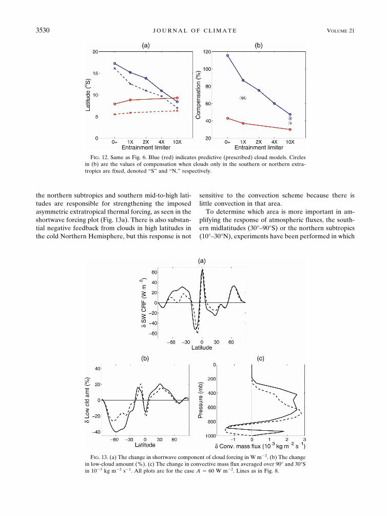
the northern subtropics and southern mid-to-high lati-tudes are responsible for strengthening the imposedasymmetric extratropical thermal forcing, as seen in theshortwave forcing plot (Fig. 13a). There is also substan-tial negative feedback from clouds in high latitudes inthe cold Northern Hemisphere, but this response is not

sensitive to the convection scheme because there islittle convection in that area.

To determine which area is more important in am-plifying the response of atmospheric fluxes, the south-ern midlatitudes (30°–90°S) or the northern subtropics(10°–30°N), experiments have been performed in which

FIG. 13. (a) The change in shortwave component of cloud forcing in W m�2. (b) The changein low-cloud amount (%). (c) The change in convective mass flux averaged over 90° and 30°Sin 10�3 kg m�2 s�1. All plots are for the case A � 60 W m�2. Lines as in Fig. 8.

FIG. 12. Same as Fig. 6. Blue (red) indicates predictive (prescribed) cloud models. Circlesin (b) are the values of compensation when clouds only in the southern or northern extra-tropics are fixed, denoted “S” and “N,” respectively.


Fig 12 live 4/C

clouds have been prescribed in only one of these areasin turn. These regions were chosen as those in which theshortwave cloud forcing and low-cloud responses inFigs. 13a and 13b are most sensitive to �. We find thateach of these regions contributes roughly half of thecloud feedback effect on the degree of tropical com-pensation C, as illustrated in Fig. 12b.

Both the reduction in low-cloud amount over thesouthern midlatitudes and the increase in low-cloudamount over the northern subtropics are sensitive to �.In the warmed Southern Hemisphere, the temperatureand humidity near the surface increase so that the at-mosphere is destabilized, thereby inducing more deepconvection, as can be seen from Fig. 13c, which showsthe change in convective mass flux averaged over 90°–30°S. Because deep convective mass flux increases atthe expense of shallow convection and drives the com-pensating subsidence, there is a reduction in convectivemass flux below 800 mb. In case of � � 1X, shallowconvection seems to become shallower as the convec-tive mass flux increases below 900 mb. Hence, increas-ing deep convection directly contributes to the reduc-tion in lower tropospheric cloud amount because deepconvection warms and dries the lower tropospherethrough the compensating subsidence. This destroyslower-level clouds and/or prevents their formation.These aspects of convection–cloud interactions arelikely to be model dependent. Deep convection occursmore frequently when � is smaller. Thus, in the south-ern midlatitudes, the smaller the value of �, the largerthe increase of deep convection and the larger the re-duction of low-cloud amount, which in turn leads tomore warming through the feedback of cloud forcingon TOA energy fluxes. The opposite changes occur inthe northern subtropics.

In the cooled Northern Hemisphere, the sensitivityof the cloud response (Fig. 13b) to deep convectionoccurs in lower latitudes than in the warmed SouthernHemisphere. Although somewhat weaker than thechanges in the Southern Hemisphere, they are evi-dently of comparable importance for the tropical re-sponses because of greater proximity to the equator.The sensitivity to convection is presumably confined tolower latitudes in the cooled hemisphere because thereis very little deep convection in the control case athigher latitudes, and imposed cooling cannot furtherdecrease deep convection.

In addition to the response to local temperaturechange, enhanced subsidence over the northern sub-tropics associated with a stronger Hadley circulation inthe cooled hemisphere can induce an increase in low-cloud amount. Thus, it is possible that the sensitivity ofthe cloud feedbacks to convection in the northern sub-

tropics is a consequence of changes in convection in thewarm Southern Hemisphere, which increase the asym-metry of the Hadley circulation and thereby inducecloud changes in the northern subtropics through in-creased subsidence. For any given �, it is difficult todetermine whether strengthening of subsidence or re-duction in deep convection due to a stabilized atmo-sphere is more important in increasing the low-cloudamount in the northern subtropics. However, our pre-scribed cloud simulations can help sort out which effectis more responsible for creating the sensitivity to �.When we prescribe clouds only in the southern extra-tropics, removing that source of feedback, the sensitiv-ity of cloud response to � in the northern subtropics isonly reduced by 30%. Therefore, we conclude that overthe northern subtropics, the sensitivity of �CRF to �shown in Fig. 8 can be attributed to the sensitivity ofdeep convection to � in response to local temperaturechanges rather than to strengthened subsidence in thedescending branch of the Hadley cell.

The dependence of the precipitation response oncloud feedbacks suggests an important way in whichuncertainties in cloud modeling can create uncertaintiesin regional responses to climatic perturbations.

5. Conclusions

In this study, the response of the ITCZ to extratrop-ical heating and cooling is investigated. An aquaplanetGCM coupled to a slab ocean is perturbed by an im-posed cross-equatorial oceanic flux. The ITCZ is dis-placed toward the warmer hemisphere. In thinkingabout the ITCZ displacement, we find it convenient tofocus also on the degree of compensation of the im-posed oceanic transport by the atmospheric energytransport in the tropics. We can relate this degree ofcompensation to the latitude of the energy flux equatorwhere the atmospheric energy transport vanishes,which provides insight into the position of the ITCZ.

This degree of compensation is relatively high(greater than 70%) in the standard configuration of themodel, and it might be tempting to conclude that a highdegree of compensation is somehow assured by the na-ture of large-scale atmospheric dynamics. However, theconvection scheme in the model can be altered to varythe degree of compensation from 47% to 115% forotherwise identical models and forcing. Simulationswith prescribed clouds have been used to show thatchanges in the cloud response to the differential heatingof the two hemispheres are primarily responsible forthis sensitivity to the convection scheme.

It is commonly observed that cloud feedbacks are asource of much of the uncertainty in estimates of global

15 JULY 2008 K A N G E T A L . 3531

mean climate responses to external forcing (Cess et al.1996). This study provides evidence that important as-pects of the regional response of climate to externalforcing are also sensitive to cloud feedbacks. The modelconfiguration utilized here can be considered as abenchmark computation that can be used to comparethis important aspect of tropical–extratropical feedbackin a wide range of GCMs. This type of model compari-son study may be very useful in helping to understandintermodel differences in the response of the tropics toice sheets, variations in meridional overturning, oraerosol forcing confined to one hemisphere.

Acknowledgments. We thank Rong Zhang, Ken Ta-kahashi, and three anonymous reviewers for very help-ful comments on earlier versions of this paper. Specialthanks to Rong Zhang for helping with the prescribedcloud simulations. This work was supported by NSFGrant ATM-0612551.

REFERENCES

Anderson, J. L., and Coauthors, 2004: The new GFDL global at-mosphere and land model AM2–LM2: Evaluation with pre-scribed SST simulations. J. Climate, 17, 4641–4673.

Broccoli, A. J., K. A. Dahl, and R. J. Stouffer, 2006: Response ofthe ITCZ to Northern Hemisphere cooling. Geophys. Res.Lett., 33, L01702, doi:10.1029/2005GL024546.

Cess, R. D., and Coauthors, 1996: Cloud feedback in atmosphericgeneral circulation models: An update. J. Geophys. Res., 101(D8), 12 791–12 794.

Chiang, J. C. H., and C. M. Bitz, 2005: Influence of high-latitudeice cover on the marine intertropical convergence zone. Cli-mate Dyn., 25, 477–496.

Frierson, D. M. W., I. M. Held, and P. Zurita-Gotor, 2006: Agray-radiation aquaplanet moist GCM. Part I: Static stabilityand eddy scale. J. Atmos. Sci., 63, 2548–2566.

Held, I. M., M. Zhao, and B. Wyman, 2007: Dynamic radiative–

convective equilibria using GCM column physics. J. Atmos.Sci., 64, 228–238.

Koutavas, A., and J. Lynch-Stieglitz, 2004: Variability of the ma-rine ITCZ over the eastern Pacific during the past 30,000years: Regional perspective and global context. The HadleyCirculation: Present, Past, and Future, H. F. Diaz and R. S.Bradley, Eds., Springer, 347–369.

Lea, D. W., D. K. Pak, L. C. Peterson, and K. A. Hughen, 2003:Synchroneity of tropical and high-latitude Atlantic tempera-tures over the last glacial termination. Science, 301, 1361–1364.

Lee, M.-I., M. J. Suarez, I.-S. Kang, I. M. Held, and D. Kim, 2008:A moist benchmark calculation for the atmospheric generalcirculation models. J. Climate, in press.

Lindzen, R. S., and A. Y. Hou, 1988: Hadley circulations for zon-ally averaged heating centered off the equator. J. Atmos. Sci.,45, 2416–2427.

Moorthi, S., and M. J. Suarez, 1992: Relaxed Arakawa–Schubert:A parameterization of moist convection for general circula-tion models. Mon. Wea. Rev., 120, 978–1002.

Neale, R. B., and B. J. Hoskins, 2000: A standard test for AGCMsincluding their physical parameterizations. I: The proposal.Atmos. Sci. Lett., 1, 101–107.

Philander, S. G. H., D. Gu, D. Halpern, G. Lambert, N.-C. Lau, T.Li, and R. C. Pacanowski, 1996: Why the ITCZ is mostlynorth of the equator. J. Climate, 9, 2958–2972.

Soden, B. J., A. J. Broccoli, and R. S. Hemler, 2004: On the use ofcloud forcing to estimate cloud feedback. J. Climate, 17,3661–3665.

Tokioka, T., K. Yamazaki, A. Kitoh, and T. Ose, 1988: The equa-torial 30–60-day oscillation and the Arakawa–Schubert pen-etrative cumulus parameterization. J. Meteor. Soc. Japan, 66,883–901.

Xie, S.-P., 2004: The shape of continents, air–sea interaction, andthe rising branch of the Hadley circulation. The Hadley Cir-culation: Present, Past, and Future, H. F. Diaz and R. S. Brad-ley, Eds., Springer, 121–152.

Zhang, M. H., J. J. Hack, J. T. Kiehl, and R. D. Cess, 1994: Diag-nostic study of climate feedback processes in atmosphericgeneral circulation models. J. Geophys. Res., 99, 5525–5537.

Zhang, R., and T. L. Delworth, 2005: Simulated tropical responseto a substantial weakening of the Atlantic thermohaline cir-culation. J. Climate, 18, 1853–1860.


the response of the itcz to extratropical thermal forcing: idealized ... · the response of the...

Documents