the response of railroad and truck freight shipments …
TRANSCRIPT
T H E R E S P O N S E O F R A I L R O A D A N D T R U C K F R E I G H T S H I P M E N T S T O
O P T I M A L E X C E S S C A PA C I T Y S U B S I D I E S A N D E X T E R N A L I T Y TA X E S
AN EMPIRICAL STUDY OF FLORIDA’S SURFACE FREIGHT TRANSPORTATION MARKET
Principal Investigator - James F. Dewey Research Economist, Economic Analysis Program
Bureau of Economic and Business Research
Senior Advisor - David Denslow Director, Economic Analysis Program
Bureau of Economic and Business Research
Research Associate – David Lenze Associate Director, Economic Analysis Program
Bureau of Economic and Business Research
Research Coordinator - Eve Irwin
Research Assistant Salvador Martinez
Publications/Information
Susan Floyd Carol Griffen
Dot Evans
September 30, 2002
U N I V E R S I T Y O F F L O R I D A
B U R E A U O F E C O N O M I C A N D B U S I N E S S R E S E A R C H
University of Florida, BEBR FDOT Contract Number B—354-44 1
The Response of Railroad and Truck Freight Shipments to Optimal Excess Capacity Subsidies and Externality Taxes
An Empirical Study of Florida’s Surface Freight Transportation Market
1. Introduction
Florida’s public highways are congested. At the same time there is excess capacity on private railroads. Further, the social costs of moving a ton-mile of freight— including costs from air pollution, accidents, congestion, and wear on the nation’s transportation system—are lower by rail than by truck for many types of freight movements. Given this situation, should the state design policies to increase utilization of the state’s railroads? Would a policy that subsidizes freight shipment by railroad, and taxes the generation of harmful externalities, be beneficial to residents of the state? This report examines whether such policies can be economically justified.
First, the extent of highway congestion is described. Second, estimates of the
social costs of freight transportation are presented. Third, the notion of excess capacity is developed and applied to railroads. Finally, the use of subsidies to exploit excess capacity is considered. The success of such a subsidy depends on the extent to which firms can and do substitute railroads for trucks in meeting their transportation demands as the relative prices of the two modes change. Because there is little agreement on the degree to which the two modes are substitutable, the issue is discussed in detail and some empirical evidence provided. We also briefly consider factors other than prices that affect modal choice.
Given this background, a framework or model for evaluating the economic
consequences of a state policy of subsidizing shipment of freight by railroad is discussed. Values for the various parameters in the model are obtained from academic research published primarily in the last twenty-five years. A review of this literature is organized around four themes: trucking cost functions, railroad cost functions, demand functions for trucking and railroads, and other studies.
We use a model constructed on this basis to determine the optimal subsidy and to
determine the shifts in freight shipments by mode that such a subsidy could achieve. Because there is less agreement on the magnitudes of the model’s parameters than is desirable, a large number of alternative simulations of the model are presented using a range of plausible values for critical parameters. These simulations convey a sense of the uncertainty attached to the analysis of the subsidy policy.
Because the social costs of freight shipment are so large, we also examine a
policy of optimal externality taxes combined with a subsidy to exploit excess capacity in the railroad industry. For interurban areas, we estimate the optimal externality taxes and the mode shifts such taxes can induce. The spatial and temporal complexity of externalities in urban areas, particularly urban congestion, precludes such estimates.
University of Florida, BEBR FDOT Contract Number B—354-44 2
Instead we indicate the data and models that need to be developed in order to quantitatively assess such policies in urban areas.
Any subsidy program would represent additional intervention by government in
private markets. Such intervention often is accompanied by unintended consequences and distortions due to the mixture of political and economic incentives. We briefly consider what light such a political-economy perspective might shed upon the desirability of a program to subsidize rail freight shipments.
The last section summarizes the findings and discusses the implications for
transportation policy in Florida. In his classic paper on the welfare cost of monopoly, Arnold Harberger (1954)
wrote: “It should be clear from the outset that this is not the kind of job one can do with great precision. The best we can hope for is to get a feeling for the general orders of magnitude that are involved.” The same applies to this study of surface freight transportation.
2. Highways are Congested It hardly seems necessary to substantiate the claim that urban highways are
congested; this is something almost anyone can verify by direct experience twice a day. Nevertheless substantial effort is devoted to the precise definition and measurement of highway congestion and a range of cross-sectional, time-series congestion measures for Florida’s five largest urbanized areas 1982-1999 are reported in The 2001 Urban Mobility Report (Schrank & Lomax, 2001).
Of the many ways to quantify congestion and to compare its level over time and
between cities, we select one measure from this report—the percent of peak-period travel under congested conditions. Peak travel periods are defined by the report as occurring between 6:00-9:30 a.m. and 3:30-7:00 p.m. Congestion is defined as occurring when speeds on freeways and principal arterial streets fall below free-flow levels. In 1999, the most recent year available, 40% of peak-period travel was in congested conditions in Jacksonville and in Miami 71% of peak-period travel was in congestion.
As graphic as such a measure is, economists prefer to define congestion as the
increase in a traveler’s travel time caused by other travelers’ use of the same transportation mode. The cost of congestion will vary from traveler to traveler according to the value of his time. The salient feature of congestion to an economist is that a driver is able to freely use the resources (time) of other travelers. For example, a driver considering whether to take a particular freeway considers only the cost to him such a choice entails. But his use of the freeway can slow the speed of other drivers, increasing the time cost of their travel. In effect, he is using up some of their time without
University of Florida, BEBR FDOT Contract Number B—354-44 3
compensation. This is one example from a broad class of costs that economists call “externalities.”
3. Shipment of Freight has External Costs The free use of resources is also the crux of the pollution problems associated
with freight shipment. Trucks and railroad engines spew noxious chemicals into the atmosphere. They generate noise. Lives are lost, injuries sustained, and property damaged in the accidents associated with their operation. To the extent that such losses are not compensated (insured), they are another form of externality.
Forkenbrock (1999, 2001) presented estimates of the average cost of some of the
externalities associated with the shipment of freight by truck and by train. The estimates are his in the sense that they were selected or computed from other published estimates.
Forkenbrock counts greenhouse gases as an externality, despite the skepticism of
the scientific community. He also treats the subsidized provision of highways to the motor carrier industry as an externality, despite the skepticism of the truck lobby.1 Since these costs are explicit and separable in Forkenbrock’s presentation, those who disagree with such treatment can easily remove them from the total the cost category in dispute. Similar estimates (as well as a critique) of the various externality costs of freight transportation can be found in Committee for Study of Public Policy for Surface Freight Transportation (1996).
The external costs Forkenbrock considers are for freight shipments in rural areas
(intercity shipments). Urban areas are ignored because air pollution costs and congestion vary substantially among cities, whereas intercity cost estimates are consistent across most rural areas.
Forkenbrock’s data refer to truckload (TL) shipments of general freight, as
distinct from less-than-truckload (LTL) shipments of general freight and truckload shipments of specialized freight.
His estimate of the private cost of freight transport consists of operating costs
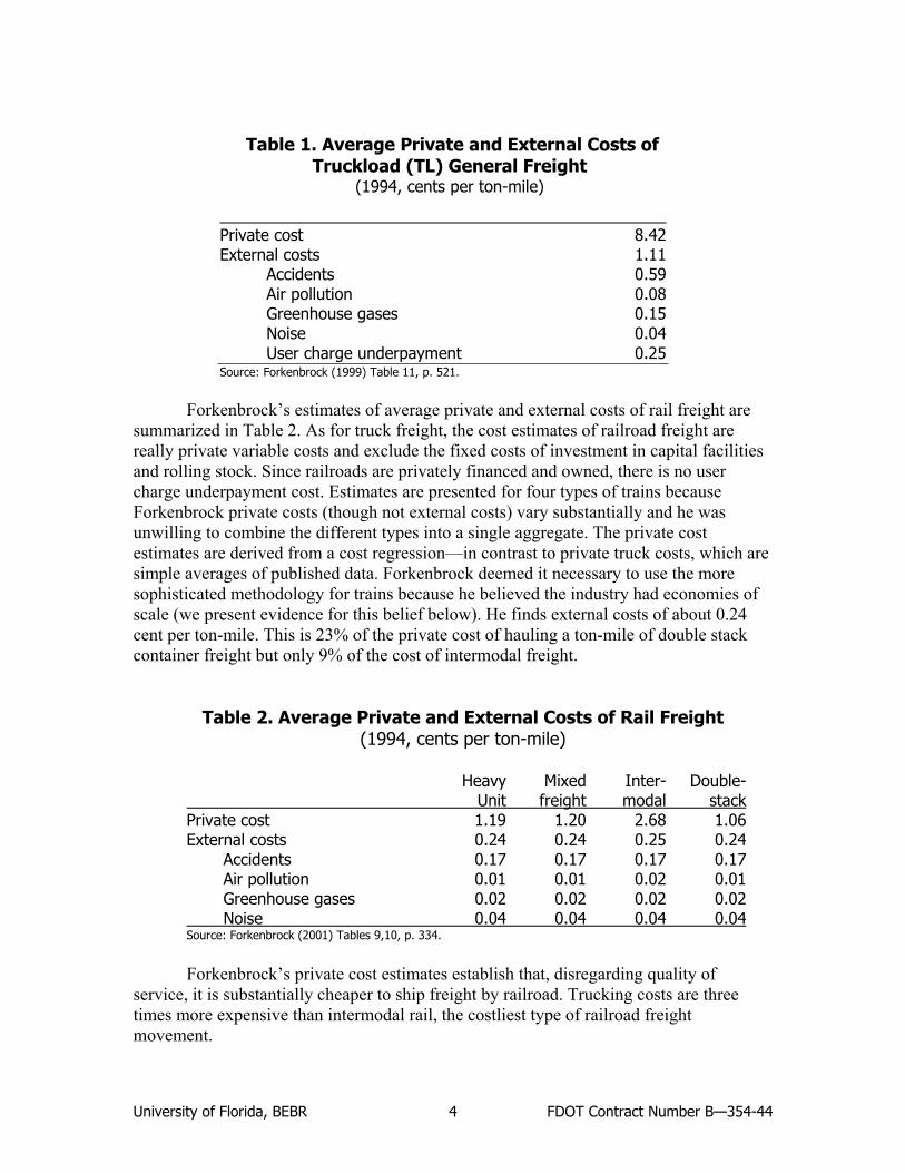
only, not the costs of buildings and rolling stock. In economic jargon Forkenbrock estimates variable costs rather than total costs (the sum of variable and fixed costs). If there are no significant economies of scale in the truckload general freight sector (i.e., if there are constant returns to scale), then average operating costs are a useful approximation of private marginal costs. Forkenbrock’s private and external costs of truckload general freight shipment are presented in Table 1. External costs of 1.11 cents per ton-mile (1994 dollars) are about 13% of the private cost.
1 The user charge underpayment represents “unrecovered costs associated with the provision, operation, and
maintenance” of highways.
University of Florida, BEBR FDOT Contract Number B—354-44 4
Table 1. Average Private and External Costs of Truckload (TL) General Freight
(1994, cents per ton-mile)
Private cost 8.42 External costs 1.11 Accidents 0.59 Air pollution 0.08 Greenhouse gases 0.15 Noise 0.04 User charge underpayment 0.25 Source: Forkenbrock (1999) Table 11, p. 521.
Forkenbrock’s estimates of average private and external costs of rail freight are
summarized in Table 2. As for truck freight, the cost estimates of railroad freight are really private variable costs and exclude the fixed costs of investment in capital facilities and rolling stock. Since railroads are privately financed and owned, there is no user charge underpayment cost. Estimates are presented for four types of trains because Forkenbrock private costs (though not external costs) vary substantially and he was unwilling to combine the different types into a single aggregate. The private cost estimates are derived from a cost regression—in contrast to private truck costs, which are simple averages of published data. Forkenbrock deemed it necessary to use the more sophisticated methodology for trains because he believed the industry had economies of scale (we present evidence for this belief below). He finds external costs of about 0.24 cent per ton-mile. This is 23% of the private cost of hauling a ton-mile of double stack container freight but only 9% of the cost of intermodal freight.
Table 2. Average Private and External Costs of Rail Freight (1994, cents per ton-mile)
Heavy Mixed Inter- Double- Unit freight modal stack Private cost 1.19 1.20 2.68 1.06 External costs 0.24 0.24 0.25 0.24 Accidents 0.17 0.17 0.17 0.17 Air pollution 0.01 0.01 0.02 0.01 Greenhouse gases 0.02 0.02 0.02 0.02 Noise 0.04 0.04 0.04 0.04 Source: Forkenbrock (2001) Tables 9,10, p. 334.
Forkenbrock’s private cost estimates establish that, disregarding quality of
service, it is substantially cheaper to ship freight by railroad. Trucking costs are three times more expensive than intermodal rail, the costliest type of railroad freight movement.
University of Florida, BEBR FDOT Contract Number B—354-44 5
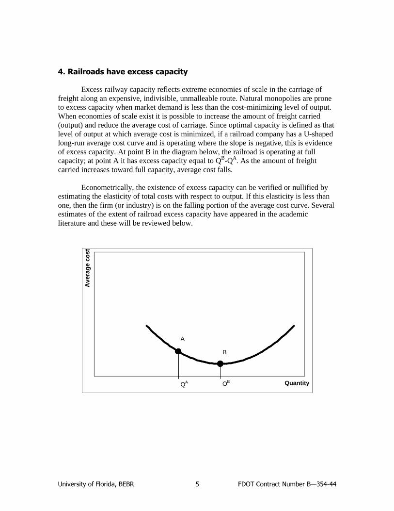
4. Railroads have excess capacity Excess railway capacity reflects extreme economies of scale in the carriage of
freight along an expensive, indivisible, unmalleable route. Natural monopolies are prone to excess capacity when market demand is less than the cost-minimizing level of output. When economies of scale exist it is possible to increase the amount of freight carried (output) and reduce the average cost of carriage. Since optimal capacity is defined as that level of output at which average cost is minimized, if a railroad company has a U-shaped long-run average cost curve and is operating where the slope is negative, this is evidence of excess capacity. At point B in the diagram below, the railroad is operating at full capacity; at point A it has excess capacity equal to QB-QA. As the amount of freight carried increases toward full capacity, average cost falls.
Econometrically, the existence of excess capacity can be verified or nullified by
estimating the elasticity of total costs with respect to output. If this elasticity is less than one, then the firm (or industry) is on the falling portion of the average cost curve. Several estimates of the extent of railroad excess capacity have appeared in the academic literature and these will be reviewed below.
Quantity
Ave
rag
e co
st
B
A
QA QB

University of Florida, BEBR FDOT Contract Number B—354-44 6
5. Subsidies to Freight Shipment by Railroad can Reduce Truck Traffic on highways
Natural monopolies require the attention of the public because they do not have
the nice efficiency properties of competitive firms. Many policies have been proposed to improve the behavior of monopolistic firms, including subsidizing their output. However, economists are unwilling to accept the mere existence of monopoly as grounds for public intervention in the marketplace. Such intervention has costs of its own which can often exceed the benefits achieved.
Proponents of subsidized shipment of freight by railroad point out that many governments currently subsidize passenger travel on transit systems in a variety of ways in order to help reduce highway congestion. The proponents claim to be merely advocating that a policy, which is evidently acceptable politically, be extended to a larger arena. Kain (1999), however, opines that these subsidies have been squandered by policymakers and transit managers who construct and operate costly and ineffective rail transit systems rather than improve bus service and reduce bus fares. A careful understanding of surface freight transportation markets is necessary so that if subsidies are justifiable on efficiency grounds, the policies chosen to implement the subsidies avoid similar errors.
6. Substitutability of Trains and Trucks A policy to encourage the shift of freight shipment from highway to railway must
take into account the substitutability of the two modes of transportation in order to succeed. Some experts aver that the two modes effectively compete only for a narrow range of shipments; some shipments (bulk commodities like coal and grain) are largely captive to railroads while other shipments (high value-to-weight manufactured goods) are largely captive to trucks. For instance, Boyer (1997, p. 58) states, “the majority of the users of truck transportation cannot easily switch to another mode of transport in response to a relative price change.” As support for this view he points out that there were no major shifts between trucking and other forms of surface transportation after trucking was deregulated. He contends that most of the manufactured goods that can be shipped by train are “intermediate goods that move in large flows between distant factories.” (1997, p. 58)
Estimating the amount of traffic that could potentially be shipped either by rail or by truck is difficult because all that the data reveal is the actual choice made, not the relevant options. One of the earliest attempts to do so was Morton (1972) who examined to what extent characteristics such as shipment size, length of haul, and value of commodity might restrict freight to one mode of transportation. Morton contrasted this
University of Florida, BEBR FDOT Contract Number B—354-44 7
approach to the orthodox method of identifying areas of intermodal competition through the use of cost functions and admitted this method might not work when it is possible to divert traffic between modes through slight technical innovations. As an example Morton indicated that the rail share of the transport of new vehicles leaving the assembly line was 8% in 1959. By 1968, it rose to 49% because of the introduction of the “tri-level auto rack.”
Despite finding that there were distinct differences in the size of shipments carried
by each mode, Morton concluded that trains and trucks compete across a broad front with respect to commodities carried and length of haul; “Either mode possesses the potential ability to divert substantial amounts of manufacturing traffic from the other.” (p. 58)
The recent development of Transportation Satellite Accounts to the national
Input-Output (IO) Accounts supports Morton’s conclusion. The Transportation Satellite Accounts are our most comprehensive measure of transportation services—they include both for hire transportation and own-account transportation as well as both intercity transportation and city delivery.2 In these accounts, transportation services are measured as expenditure—that is, as the product of quantity of service and price per unit of service. This enhances comparability between industries and between other inputs.
Input-Output tables are usually faulted for assuming fixed proportions in
production and for assuming static technology. However, we will not use a single IO table to predict the economic consequences of alternative transportation policies, nor will we use a single IO table to predict the future. Instead, we will examine how the Transportation Satellite Accounts changed over a four-year period, circumventing the two faults just mentioned. The “Use Table” for 1992 describes the technology (e.g., input requirements) each industry used that year. The “Use Table” for 1996 describes the technology used in that year. We are interested in how technology has changed between 1992 and 1996 and the relation between relative price changes and the relative use of transportation modes.
Perhaps the most interesting fact about the Transportation Satellite Accounts is that every one of its industries (there are 93) purchases transportation services from both railroad and trucking companies.3 So there appears to be substitution possibilities in
2 The IO Accounts recognize purchases and sales of transportation services of “for-hire” transportation firms only.
However, some firms own and operate trucks on their own account rather than (or, as well as) purchase service from for-hire firms. The Transportation Satellite Accounts introduce a new commodity into the IO Accounts, “own-account transportation,” for such activities. In the IO Accounts, the use of for-hire transportation by an industry includes only those transportation expenses associated with moving intermediate inputs to the industry plus the expenses for certain direct use of transportation commodities. The same is true of the Transportation Satellite Accounts. However, in the Transportation Satellite Accounts, all own-account transportation is attributed to the industry that owns the trucks even if they are used to haul away output.
3 Since general government and households are exogenous, their transportation demands are excluded from the Use Table. The railroad industry in the Transportation Satellite Accounts contains buses and passenger trains as well as freight trains. The IO Accounts separate freight transportation from these other categories. Of the 491 industries in the IO Accounts, 423 purchase transportation services from the narrowly-defined railroad freight industry.
University of Florida, BEBR FDOT Contract Number B—354-44 8
every industry, even if there may not be much possibility at the firm level in the short run. It is true that individual establishments (e.g., a particular manufacturing plant) may rely solely on one mode of transportation and so have essentially no room for substitution of trains for trucks in the short-run as relative prices change. However, at the industry level the Transportation Satellite Accounts indicate room for such substitution. For instance, as relative prices change favoring one transportation mode over another, the market may allocate more demand to those manufacturing plants that have access to the now cheaper transport mode. Comparison of the 1992 and 1996 accounts shows that, in fact, most industries did increase their use of trains in response to relatively high price increases for shipment by truck.
This is witnessed when the expenditure data in the Transportation Satellite
Accounts is transformed into quantity measures by using price indexes. Before doing so, two issues must be addressed. First, price indexes are available only for the aggregate output of the railroad and truck industries. It is well known that shipment rates vary substantially by commodity; the rate per ton railroads charge to carry coal is much lower than the rate they charge to haul automobiles. However, it seems reasonable to suppose that despite big differences in transport price levels between commodities, changes in those levels over a very short period are probably very similar across all commodities (especially since there have been no major innovations within specific sectors of the trucking and railroad industries, nor any major deregulation of specific sectors, etc.). Second, we were unable to find a price index for truckload shipments and, therefore, use an index for less-than-truckload shipments as a proxy.4 Again, we appeal to the reasonableness of the assumption that over a short period of time, price changes in most trucking sectors are likely to be similar.
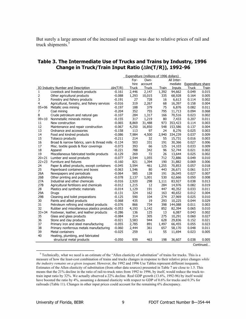
In Table 3, we present expenditure data by industry from the 1996 Transportation
Account, the most recent Account available. Expenditure is tabulated for for-hire truck, own-account truck, trains, and all intermediate inputs. The 1996 expenditure for trucks (both for-hire and own-account) and for trains as a percentage of expenditure on all intermediate inputs is provided in the last two columns. The change in the relative usage of trains and trucks from 1992 to 1996 (the column labeled ∆lnT/R) is computed as the logarithmic change in the ratio of trucking expenditure to railroad expenditure, both deflated by their respective price indices.
Rail rates fell on average 8.9% while truck rates rose 12.6%. Relative price
changes clearly discouraged the use of trucks and, in fact, we can see from this table that most industries did reduce their use of trucks relative to trains, often by substantial amounts. Of course, things other than relative rail and truck rate changes played a role in the changed input ratios. For one thing, GDP grew substantially as the economy recovered from the 1990-91 recession and the relative prices of other inputs also changed.
4 The data are from Wilson (1999, p. 49).
University of Florida, BEBR FDOT Contract Number B—354-44 9
But surely a large amount of the increased rail usage was due to relative prices of rail and truck shipments.5
Table 3. The Intermediate Use of Trucks and Trains by Industry, 1996 Change in Truck/Train Input Ratio (∆ln(T/R)), 1992-96
Expenditure (millions of 1996 dollars) For- Own- All Inter- hire account mediate Expenditure share IO Industry Number and Description ∆ln(T/R) Truck Truck Train Inputs Truck Train 1 Livestock and livestock products -0.161 2,446 2,147 1,392 94,662 0.049 0.015 2 Other agricultural products -0.088 1,293 10,015 335 68,928 0.164 0.005 3 Forestry and fishery products -0.191 27 728 16 6,613 0.114 0.002 4 Agricultural, forestry, and fishery services -0.016 319 2,267 68 16,397 0.158 0.004 05+06 Metallic ores mining -0.197 188 379 75 6,876 0.082 0.011 7 Coal mining -0.204 352 755 795 11,713 0.094 0.068 8 Crude petroleum and natural gas -0.107 284 1,317 166 70,516 0.023 0.002 09+10 Nonmetallic minerals mining -0.155 317 1,219 80 7,433 0.207 0.011 11 New construction -0.065 8,869 31,488 973 353,423 0.114 0.003 12 Maintenance and repair construction -0.067 4,250 16,850 548 153,586 0.137 0.004 13 Ordnance and accessories -0.158 113 97 24 8,276 0.025 0.003 14 Food and kindred products -0.086 7,984 4,500 2,940 334,239 0.037 0.009 15 Tobacco products -0.211 214 32 55 15,731 0.016 0.003 16 Broad & narrow fabrics, yarn & thread mills -0.134 503 331 191 30,366 0.027 0.006 17 Misc. textile goods & floor coverings -0.073 393 66 125 14,103 0.033 0.009 18 Apparel -0.221 788 342 96 52,744 0.021 0.002 19 Miscellaneous fabricated textile products -0.129 269 72 26 13,644 0.025 0.002 20+21 Lumber and wood products -0.077 2,544 1,055 712 72,886 0.049 0.010 22+23 Furniture and fixtures -0.160 821 1,394 190 31,882 0.069 0.006 24 Paper & allied products, except containers -0.045 3,594 461 1,255 70,853 0.057 0.018 25 Paperboard containers and boxes -0.063 1,546 80 443 26,671 0.061 0.017 26A Newspapers and periodicals -0.064 585 128 191 26,045 0.027 0.007 26B Other printing and publishing -0.078 2,137 1,001 530 62,666 0.050 0.008 27A Industrial and other chemicals -0.016 2,920 298 1,111 83,927 0.038 0.013 27B Agricultural fertilizers and chemicals -0.012 1,215 12 284 14,976 0.082 0.019 28 Plastics and synthetic materials -0.014 1,129 191 447 40,352 0.033 0.011 29A Drugs -0.131 324 162 163 40,652 0.012 0.004 29B Cleaning and toilet preparations -0.125 590 104 274 27,969 0.025 0.010 30 Paints and allied products -0.068 435 19 293 10,225 0.044 0.029 31 Petroleum refining and related products -0.076 866 734 398 144,088 0.011 0.003 32 Rubber and miscellaneous plastics products -0.053 4,193 1,142 852 82,394 0.065 0.010 33+34 Footwear, leather, and leather products -0.286 136 125 13 6,087 0.043 0.002 35 Glass and glass products -0.084 314 305 275 10,291 0.060 0.027 36 Stone and clay products -0.021 3,583 944 628 29,836 0.152 0.021 37 Primary iron and steel manufacturing -0.055 2,785 891 1,497 66,455 0.055 0.023 38 Primary nonferrous metals manufacturing -0.060 2,444 361 657 58,170 0.048 0.011 39 Metal containers -0.025 259 11 55 11,694 0.023 0.005 40 Heating, plumbing, and fabricated structural metal products -0.050 939 463 198 36,607 0.038 0.005
Continued…
5 Technically, what we need is an estimate of the “Allen elasticity of substitution” of trains for trucks. This is a
measure of how the least-cost combination of trains and trucks changes in response to their relative price changes while the industry remains on a given isoquant. However, the 1992 and 1996 Use Tables represent different isoquants. Estimates of the Allen elasticity of substitution (from other data sources) presented in Table 7 are close to 1.5. This means that the 21% decline in the ratio of rail-to-truck rates from 1992 to 1996, by itself, would reduce the truck-to-train input ratio by 32%. We actually observed a 22% decline. Real GDP growth (13.6%, 1992-96) by itself would have boosted the ratio by 4%, assuming a demand elasticity with respect to GDP of 0.6% for trucks and 0.3% for railroads (Table 11). Changes in other input prices could account for the remaining 6% discrepancy.
University of Florida, BEBR FDOT Contract Number B—354-44 10
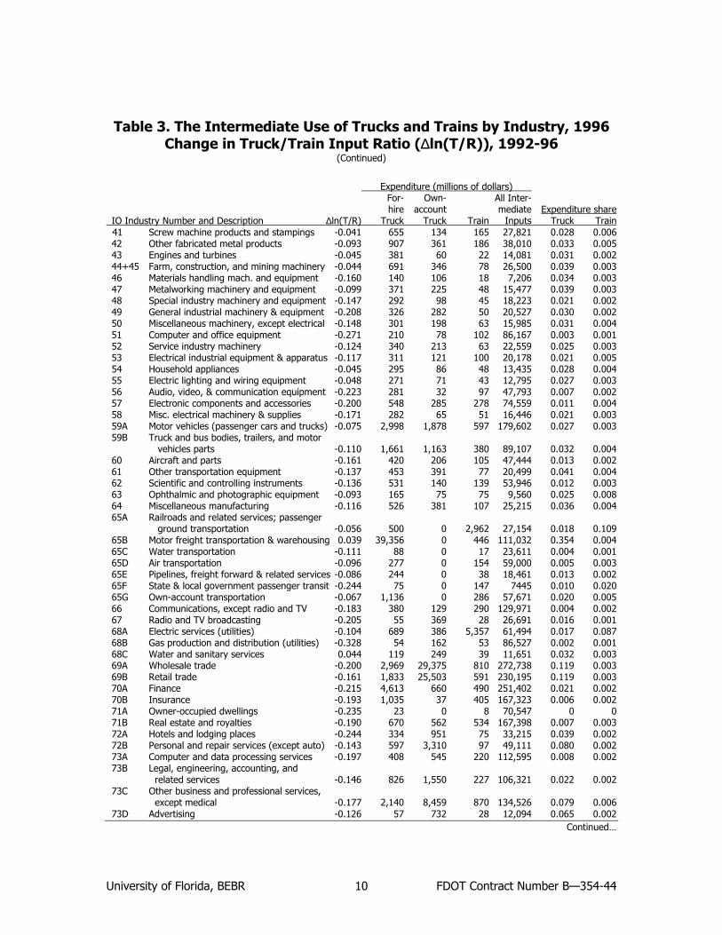
Table 3. The Intermediate Use of Trucks and Trains by Industry, 1996 Change in Truck/Train Input Ratio (∆ln(T/R)), 1992-96
(Continued)
Expenditure (millions of dollars) For- Own- All Inter- hire account mediate Expenditure share IO Industry Number and Description ∆ln(T/R) Truck Truck Train Inputs Truck Train 41 Screw machine products and stampings -0.041 655 134 165 27,821 0.028 0.006 42 Other fabricated metal products -0.093 907 361 186 38,010 0.033 0.005 43 Engines and turbines -0.045 381 60 22 14,081 0.031 0.002 44+45 Farm, construction, and mining machinery -0.044 691 346 78 26,500 0.039 0.003 46 Materials handling mach. and equipment -0.160 140 106 18 7,206 0.034 0.003 47 Metalworking machinery and equipment -0.099 371 225 48 15,477 0.039 0.003 48 Special industry machinery and equipment -0.147 292 98 45 18,223 0.021 0.002 49 General industrial machinery & equipment -0.208 326 282 50 20,527 0.030 0.002 50 Miscellaneous machinery, except electrical -0.148 301 198 63 15,985 0.031 0.004 51 Computer and office equipment -0.271 210 78 102 86,167 0.003 0.001 52 Service industry machinery -0.124 340 213 63 22,559 0.025 0.003 53 Electrical industrial equipment & apparatus -0.117 311 121 100 20,178 0.021 0.005 54 Household appliances -0.045 295 86 48 13,435 0.028 0.004 55 Electric lighting and wiring equipment -0.048 271 71 43 12,795 0.027 0.003 56 Audio, video, & communication equipment -0.223 281 32 97 47,793 0.007 0.002 57 Electronic components and accessories -0.200 548 285 278 74,559 0.011 0.004 58 Misc. electrical machinery & supplies -0.171 282 65 51 16,446 0.021 0.003 59A Motor vehicles (passenger cars and trucks) -0.075 2,998 1,878 597 179,602 0.027 0.003 59B Truck and bus bodies, trailers, and motor vehicles parts -0.110 1,661 1,163 380 89,107 0.032 0.004 60 Aircraft and parts -0.161 420 206 105 47,444 0.013 0.002 61 Other transportation equipment -0.137 453 391 77 20,499 0.041 0.004 62 Scientific and controlling instruments -0.136 531 140 139 53,946 0.012 0.003 63 Ophthalmic and photographic equipment -0.093 165 75 75 9,560 0.025 0.008 64 Miscellaneous manufacturing -0.116 526 381 107 25,215 0.036 0.004 65A Railroads and related services; passenger ground transportation -0.056 500 0 2,962 27,154 0.018 0.109 65B Motor freight transportation & warehousing 0.039 39,356 0 446 111,032 0.354 0.004 65C Water transportation -0.111 88 0 17 23,611 0.004 0.001 65D Air transportation -0.096 277 0 154 59,000 0.005 0.003 65E Pipelines, freight forward & related services -0.086 244 0 38 18,461 0.013 0.002 65F State & local government passenger transit -0.244 75 0 147 7445 0.010 0.020 65G Own-account transportation -0.067 1,136 0 286 57,671 0.020 0.005 66 Communications, except radio and TV -0.183 380 129 290 129,971 0.004 0.002 67 Radio and TV broadcasting -0.205 55 369 28 26,691 0.016 0.001 68A Electric services (utilities) -0.104 689 386 5,357 61,494 0.017 0.087 68B Gas production and distribution (utilities) -0.328 54 162 53 86,527 0.002 0.001 68C Water and sanitary services 0.044 119 249 39 11,651 0.032 0.003 69A Wholesale trade -0.200 2,969 29,375 810 272,738 0.119 0.003 69B Retail trade -0.161 1,833 25,503 591 230,195 0.119 0.003 70A Finance -0.215 4,613 660 490 251,402 0.021 0.002 70B Insurance -0.193 1,035 37 405 167,323 0.006 0.002 71A Owner-occupied dwellings -0.235 23 0 8 70,547 0 0 71B Real estate and royalties -0.190 670 562 534 167,398 0.007 0.003 72A Hotels and lodging places -0.244 334 951 75 33,215 0.039 0.002 72B Personal and repair services (except auto) -0.143 597 3,310 97 49,111 0.080 0.002 73A Computer and data processing services -0.197 408 545 220 112,595 0.008 0.002 73B Legal, engineering, accounting, and related services -0.146 826 1,550 227 106,321 0.022 0.002 73C Other business and professional services, except medical -0.177 2,140 8,459 870 134,526 0.079 0.006 73D Advertising -0.126 57 732 28 12,094 0.065 0.002 Continued…

University of Florida, BEBR FDOT Contract Number B—354-44 11
Table 3. The Intermediate Use of Trucks and Trains by Industry, 1996 Change in Truck/Train Input Ratio (∆ln(T/R)), 1992-96
(Continued)
Expenditure (millions of dollars) For- Own- All Inter- hire account mediate Expenditure share IO Industry Number and Description ∆ln(T/R) Truck Truck Train Inputs Truck Train 74 Eating and drinking places -0.083 2,559 12,520 561 175,078 0.086 0.003 75 Automotive repair and services 0.023 1,084 3,884 359 95,915 0.052 0.004 76 Amusements -0.237 386 3,063 147 80,769 0.043 0.002 77A Health services -0.203 2,108 6,957 939 260,341 0.035 0.004 77B Educational and social services, and membership organizations -0.208 1,109 9,946 318 142,370 0.078 0.002 78 Federal government enterprises 0.053 1,690 823 764 25,146 0.100 0.030 79 State and local government enterprises 0.096 727 0 502 51,033 0.014 0.010 Maximum 0.096 39,356 31,488 5,357 353,423 0.354 0.109 Minimum -0.328 23 0 8 6,087 0 0 Source: Expenditure data are from the Transportation Satellite Accounts. The input ratio is computed from the expenditure data using price indexes from Wilson (1999, p. 49).
As a consequence, real expenditure on trains as an intermediate input in
production rose 32% (1992-96) while the comparable expenditure on trucks rose only 10%. Given that trucks dominate trains as an input—firms spent more than $8 on trucking services for every $1 spent on train services in 1996—it would take many years of similar relative price changes before railroads begin to collect as much revenue as trucks. Nevertheless, it is interesting to note that price changes 1997-2001 continue to favor railroads. The producer price index published by the U.S. Department of Labor indicates that over this period trucking prices rose 13.2% while railroad prices rose only 4.3%.6
In summary, the evidence suggests ample substitutability between trucks and
trains across most industries, providing hope that a subsidy to rail shipment may actually shift a substantial amount of freight from the highways to the railways.
7. Factors Affecting Modal Choice In addition to the prices of shipping freight by the various modes available, there
are many other matters considered by shippers in the choice of transportation mode. Researchers have emphasized different factors in their studies depending on their objectives and the availability of data. For instance, Levin (1978) mentions: (1) transit time or speed (there is an inventory cost while a good is in transit between the seller and the buyer); (2) size of shipment (there are economies of scale; a railcar typically can carry more than a trailer pulled by a truck); (3) damage to or loss of shipment; (4) reliability
6 The series ID for “Railroad transportation” is PCU40 and the series ID for “Trucking and courier services, except
air” is PCU421.

University of Florida, BEBR FDOT Contract Number B—354-44 12
(variation in pick-up and delivery time); and 5) flexibility (the availability of custom shipment services for the shipper and recipient).
Other considerations reflect the characteristics of the freight itself (perish ability,
fragility, and weight) or characteristics of the shipper (location and past transport demand).
Winston et al. (1990, p. 27) mention three other dimensions of service important
to modal choice: (1) time between a shipper’s request for service and the arrival of a carrier at the dock; (2) the ability to specify equipment type along with the contractual freight rate; and (3) frequency of service (a higher frequency allows shippers to transport smaller shipments and hold down inventory costs).
8. A Model of the Freight Transportation Market: Preliminaries Evaluation of a freight subsidy requires a model of the surface freight
transportation market. More than twenty years ago two economists associated with the Massachusetts Institute of Technology, Ann Friedlaender and Richard Spady, estimated such a model and published the results of their five-year undertaking in a much-cited book Freight Transport Regulation (1981). The general framework of their study is still relevant today and we will use it as a starting-point for the current study.
Friedlaender and Spady’s (1981) general framework can be succinctly described.
They built a general equilibrium model of freight transportation consisting of two modes of transportation (trains and trucks), two types of hauled commodities (manufactures and bulk), two regions (the “Official Territory” and the “South and West”), and two models of regional output.
The market for hauling each commodity by each transportation mode in each
region consisted of two equations, one representing market demand, and the other representing market supply. The models of regional output, in principle, allow changes in the six transportation markets to affect all other markets (treated for simplicity as a single all other market) as well as to be affected by changes in these other markets. In this sense, they have built a general equilibrium model of the entire economy.
Their model implicitly assumed that prices of labor, capital, and intermediate
goods used by trucks and railroads were constant so that changes in the output of these industries could be treated as a slide along a given cost curve. If input prices varied with the scale of the industry, the analysis would have to be modified. Their model also ignores competition with other modes of freight transportation, such as pipelines, barges, and airlines.
University of Florida, BEBR FDOT Contract Number B—354-44 13
Although this framework is still valid today, we cannot use their estimates in our study because, among others things, it was estimated with very old data. For instance, the data for railroads was from 1968-70. Not only has transportation technology changed substantially since then, but the regulatory framework has changed radically as well. Given the regulation that existed during the period they studied, it was reasonable for them to work with short-run cost curves. In today’s deregulated environment it is more appropriate to work with long-run costs.
In addition, some of their estimates seem peculiar. For example, the short-run
marginal cost curves they estimated for railroads were above the average cost curves at the mean of their sample (the point of approximation), while the estimated long-run marginal cost curves for trucks were below average costs. This implies increasing average costs in railroads and decreasing average costs in trucking. For the purposes of our study it would seem more reasonable and more consistent with recent empirical work to expect decreasing average costs for railroads, and constant average costs for trucking—at least for the truckload specialized freight sector which competes with trains.
9. Advances in Transportation Market Modeling: From Friedlaender and Spady to the Present
In this section we will review the better studies that have appeared in the
academic literature with an emphasis on those studies appearing subsequent to the 1981 Friedlaender and Spady study. As far as we are aware, no one since them has built a full general equilibrium model for analyzing transportation issues. Rather, progress has been made on specifying and estimating the individual transportation market demand and supply curves. In this review we will first make some general observations and then discuss: (1) cost functions for the trucking industry; (2) cost functions for the railroad industry; (3) demand functions for trucking and railroad transportation services; and (4) various miscellaneous studies.
Little consensus exists in the academic literature on transportation markets,
especially on empirical matters. Generally, there is agreement that the translog functional form is the best form for estimating cost functions. There are two major empirical approaches for demand functions: factor share equations derived from cost functions and qualitative choice models estimated with disaggregate data. Small and Winston (1999) prefer the latter approach but Oum, Waters, and Yong (1992) point out that when the ultimate interest is in aggregate behavior—as it is in the current study—results from the disaggregate model must still be aggregated, there is no agreement on the best manner of aggregation, and all aggregation methods generate error.
Nor is there much agreement in the academic literature about returns to scale in
trucking and railroads. There are a wide range of published price elasticities of supply and demand and even wider disagreement about cross-price elasticities.
University of Florida, BEBR FDOT Contract Number B—354-44 14
In contrast to the lack of empirical agreement there is more agreement about
theoretical matters. The basic general equilibrium framework used by Friedlaender and Spady (1981) is a well-established tool for evaluating transportation policies. There is widespread agreement that taxes and subsidies can be used to efficiently remedy the problem of externalities and excess capacity. Nevertheless, disagreements remain on other theoretical matters. Some economists prefer to use compensating variations to measure welfare changes while others prefer consumer and producer surplus measures (or some other alternative). Some economists are willing to evaluate efficiency aspects of policy independent of distributional aspects while others are not. (We will opt for consumer and producer surplus and for ignoring the income distribution.)
Economists do not speak with a single voice on matters of transportation policy.
Although no one (of whom we are aware) advocates a return to transportation rate regulation as practiced by the Interstate Commerce Commission, some economists are willing to subsidize railroads to eliminate excess capacity while others prefer Ramsey prices—the price a monopolist would charge if its profit rate were regulated by the state.
A. Cost Functions—Trucking Industry Empirical studies of the trucking industry have found it difficult to adequately
handle the substantial heterogeneity of its several segments. Unlike railroad companies, which carry an extremely wide range of commodities, motor carrier companies tend to specialize in just one line. There are many ways to classify the activities of this industry: truckload vs. less-than-truckload; for-hire vs. own-account; city delivery vs. interurban transport; common carriers vs. contract carriers; and general freight vs. specialized freight. Technology, costs, and substitutability with railroads can very substantially among the different trucking segments. For instance, the less-than-truckload general freight segment typically has higher costs than other segments of the industry because of its warehousing and terminal operations.
Forkenbrock (1999) says, “because of large investment in terminal operations,
entry into LTL operations is difficult.” (p. 508) It is possible that this might be a source of increasing returns to scale and oligopolistic behavior. On the other hand he says, “The TL market is quite easy to enter because all that is needed is a driver, rolling stock, and a freight broker with whom to work. Accordingly, the TL sector is highly fragmented, being composed of many small and medium size carriers.” (p. 508) In other words, this sector is likely to be characterized by constant marginal costs and purely competitive firm behavior.
Despite the frequent occurrence of statements such as Forkenbrock’s, it is very
difficult to establish empirically whether a particular segment has increasing, decreasing or constant costs. On the one hand, there are too few observations for some trucking
University of Florida, BEBR FDOT Contract Number B—354-44 15
segments to estimate a cost function while pooling observations across segments runs the risk of +aggregation bias.7
Much of the academic work on the trucking industry has been on the less-than-
truckload segment. As we will discuss below in the section entitled Demand Functions, there is general agreement that railroads are not a close substitute for trucks for less-than-truckload freight shipments. We therefore restrict our review of the literature to other segments.
For our purposes, the two better studies of trucking industry costs are
Friedlaender and Spady (1981) and Grimm, Corsi, and Jarrell (1989). These will be discussed in detail below. Although the former study found increasing returns to scale, the more recent study found that the trucking segments competitive with railroads have a horizontal supply (or marginal cost) curve reflecting a technology with constant returns to scale. An even more recent study by Winston et al. (1990, p. 34, fn. 47) also found constant returns to scale when they used a flexible translog cost function.
(1) Friedlaender and Spady (1981 pp. 47-60). Friedlaender and Spady (1981)
report that “proponents of regulation argue that common carrier trucking is subject to substantial economies of scale, and point to the large number of trucking mergers that have taken place in recent years as supporting evidence.” (p. 10)
Friedlaender and Spady used a sample of 362 motor carrier companies in 1972 to
estimate a total cost function. These companies were classified as carriers of “specialized commodities, not elsewhere classified.” They used ton-miles for output and controlled for average length of haul, average insurance payments (a proxy for the type of commodity hauled), and average load per vehicle. They were surprised to find economies of scale—the elasticity of total cost with respect to output was 0.8 in the Official region and 0.9 in the South-West region at the point of approximation. However, they attribute the economies of scale to “regulation” rather than to technology (p. 45). In contrast, Christensen and Huston (1987) criticize their sample as extremely heterogeneous and suggest that the finding of economies of scale was due to aggregation bias.
Friedlaender and Spady also estimated total cost functions for less-than-truckload
general commodities. In this case they found diseconomies of scale. The elasticity of total cost with respect to output was 1.1 in both the Official region the South-West region at the point of approximation (Table C. 6, p. 26). For interregional carries they estimated the elasticity to be 0.9 (Table C. 7, p. 268).
(2) Grimm, Corsi, and Jarrell (1989). The motivation for the research of Grimm,
Corsi, and Jarrell (1989) is the observation that each segment of the trucking industry has a distinct production technology: equipment differs, loading and unloading techniques
7 Surprisingly, no one seems to have succeeded in pooling data across time and adding a time trend to control for
productivity change. Such pooling has been successful with railroads.
University of Florida, BEBR FDOT Contract Number B—354-44 16
differ, and the usage of terminals differs. They hypothesized that pooling firms from all segments (as Friedlaender and Spady did) would cause severe aggregation bias in empirical work. This led them to estimate separate cost functions.
Grimm, Corsi, and Jarrell concluded that all segments of the trucking industry—
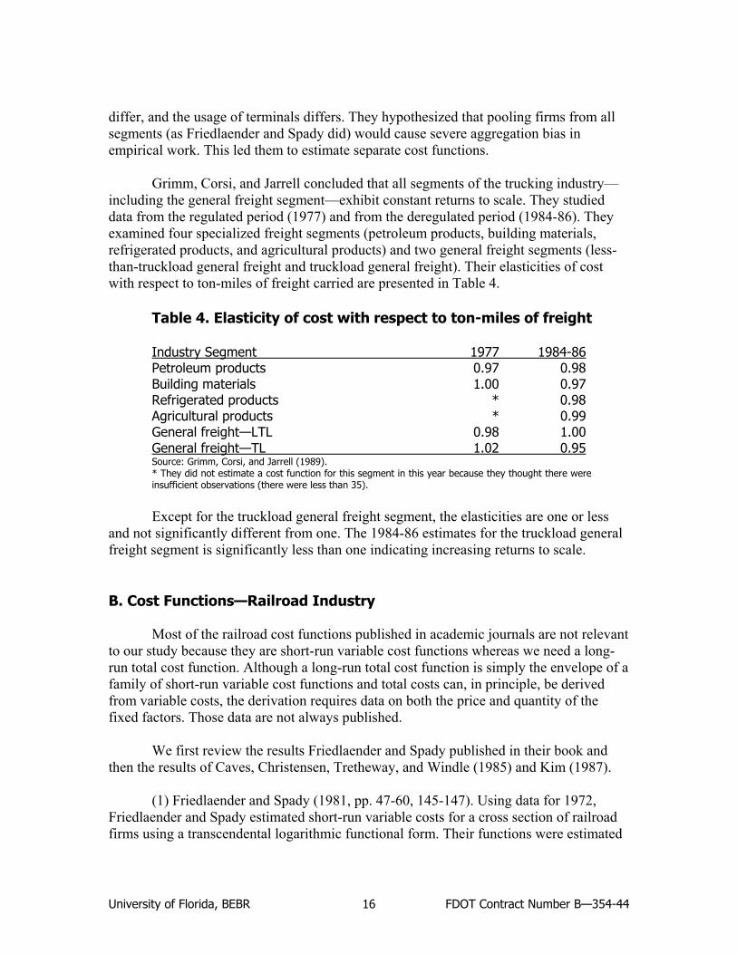
including the general freight segment—exhibit constant returns to scale. They studied data from the regulated period (1977) and from the deregulated period (1984-86). They examined four specialized freight segments (petroleum products, building materials, refrigerated products, and agricultural products) and two general freight segments (less-than-truckload general freight and truckload general freight). Their elasticities of cost with respect to ton-miles of freight carried are presented in Table 4.
Table 4. Elasticity of cost with respect to ton-miles of freight Industry Segment 1977 1984-86 Petroleum products 0.97 0.98 Building materials 1.00 0.97 Refrigerated products * 0.98 Agricultural products * 0.99 General freight—LTL 0.98 1.00 General freight—TL 1.02 0.95 Source: Grimm, Corsi, and Jarrell (1989). * They did not estimate a cost function for this segment in this year because they thought there were insufficient observations (there were less than 35).
Except for the truckload general freight segment, the elasticities are one or less
and not significantly different from one. The 1984-86 estimates for the truckload general freight segment is significantly less than one indicating increasing returns to scale.
B. Cost Functions—Railroad Industry Most of the railroad cost functions published in academic journals are not relevant
to our study because they are short-run variable cost functions whereas we need a long-run total cost function. Although a long-run total cost function is simply the envelope of a family of short-run variable cost functions and total costs can, in principle, be derived from variable costs, the derivation requires data on both the price and quantity of the fixed factors. Those data are not always published.
We first review the results Friedlaender and Spady published in their book and
then the results of Caves, Christensen, Tretheway, and Windle (1985) and Kim (1987). (1) Friedlaender and Spady (1981, pp. 47-60, 145-147). Using data for 1972,
Friedlaender and Spady estimated short-run variable costs for a cross section of railroad firms using a transcendental logarithmic functional form. Their functions were estimated

University of Florida, BEBR FDOT Contract Number B—354-44 17
separately for manufactured goods and for bulk goods in two regions. They found that the price of shipping manufactured goods by railroad was below marginal cost in both the Official and the South-West regions while the price of shipping bulk goods was above marginal cost. This strange result was contrary to the stylized fact of the time that regulation by the Interstate Commerce Commission (ICC) subsidized the shipment of farm products at the expense of manufacturers.
More relevant for our purposes is their calculation of the elasticity of long-run
total costs with respect to shipments. Their estimate of 0.8655 (pp. 145-146) indicates increasing returns to scale.
(2) Caves, Christensen, Tretheway, and Windle (1985). Using data for 1951-75,
Caves, Christensen, Tretheway, and Windle (1985) estimated that the elasticity of total costs with respect to ton-miles of freight traffic was about 0.5 when the cost function was evaluated at the average of their sample of railroads. This means that marginal costs are less than average costs and hence, average costs will fall if output expands. Using their data and again evaluating at the mean we computed the elasticity of marginal cost with respect to freight traffic to be -0.5. This means that if freight traffic expands by 10% then marginal costs will fall by 5% (holding factor prices constant as well as average length of haul, and all other variables).
It may be objected that an elasticity computed from such old data is not relevant
to the railroad industry in the 21st century. The ICC heavily regulated the railroads in their sample. They were compelled to maintain substantial excess capacity. The more numerous railroad companies back then were much smaller than the four remaining major railroads today. Today’s railroads may have exhausted economies of scale. It is reassuring to report that this estimated elasticity can be confirmed by a more recent study by Ivaldi and McCullough (2001).
Ivaldi and McCullough (2001) estimated a short run variable cost function using
data for 1978-97. Clearly, most of their data is for the period since railroads were deregulated and allowed to optimize their capital stock. Another attractive feature of their paper is that they looked at three types of output–bulk, general, and intermodal freight. (Their unit of freight output however, is car-miles rather than the ton-miles used by Caves et al.) They estimated the elasticity of marginal costs to be -0.6 for general freight, -0.3 for bulk freight, and +0.3 for intermodal freight. The positive elasticity for intermodal freight is puzzling, but we have no direct need for such an estimate. The main point is that their short-run elasticity for general freight indicates increasing returns to scale. Since the elasticity can only become more negative when moving from the short run to the long run, we would expect to find increasing returns to scale in the long run if we had the necessary data to compute it from their short-run estimates.
(3) Kim (1987). Kim (1987) estimated a total cost function for railroads using
data for 56 railroads in 1963. He estimated the elasticity of marginal cost with respect to

University of Florida, BEBR FDOT Contract Number B—354-44 18
freight shipments to be -0.37. Interestingly, he also estimated the elasticity of marginal cost of freight shipment with respect to passenger travel to be +0.166 (and the elasticity of marginal cost of passenger travel with respect to freight shipment to be +0.780). Kim explains that the diseconomy of scale arises because passenger trains and freight trains interfere with each other’s operation. The different speeds at which they optimally operate cause scheduling problems and the track maintenance requirements are different.
C. Demand Functions—Trucking & Railroads The transportation demand models of Oum (1979b) and Friedlaender and Spady
(1980, 1981), derived from cost functions, are perhaps the most attractive of those published in the academic literature. The reduced form approach used by Morton (1969) is very crude while the qualitative choice models of Boyer (1977), Levin (1978, 1981) and Winston (1981) suffer from the devastating critique of Oum (1979a). Small and Winston (1999) in contrast, think that the “disaggregate models… have generally been the most successful in capturing essential features of travel behavior.” (p. 12) This disagreement is partly over whether one’s primary interest is in aggregate or disaggregate behavior. In this study we are interested in aggregate behavior.
(1) Friedlaender and Spady (1980). Friedlaender and Spady (1980) estimated
transportation share equations derived from the cost functions of a sample of manufacturing industries using data from the Census of Transportation and calculated factor demand elasticities for railroad and trucking transportation services from these equations. It turned out that the less-than-truckload general freight segment dominated the trucking data from the Census of Transportation. They used value of shipments as a proxy for the output of the manufacturing industries. Hence, the elasticities of demand for transportation can be treated as “partial” or “compensated” or “output-constant” price elasticities. Their “all regions” results for 1972 are summarized in Table 5. These are abstracted from their Table 2, which also has estimates for five regions.
Table 5. Rail and Truck Price Elasticities Own-price elasticity Cross-price elasticity Rail Truck Truck-Rail Rail-Truck Food products -2.6 -1.0 +0.004 -0.023 Wood & wood products -2.0 -1.5 -0.129 -0.050 Paper, plastic, & rubber products -1.8 -1.1 +0.003 +0.007 Stone, clay, & glass products -1.7 -1.0 +0.016 +0.025 Iron & steel products -2.5 -1.1 -0.013 -0.053 Fabricated metal products -2.2 -1.4 -0.099 -0.059 Nonelectrical machinery -2.3 -1.1 -0.010 -0.032 Electrical machinery -3.5 -1.2 -0.061 -0.151 Source: Friedlaender and Spady (1980) Table 2, p. 439.
University of Florida, BEBR FDOT Contract Number B—354-44 19
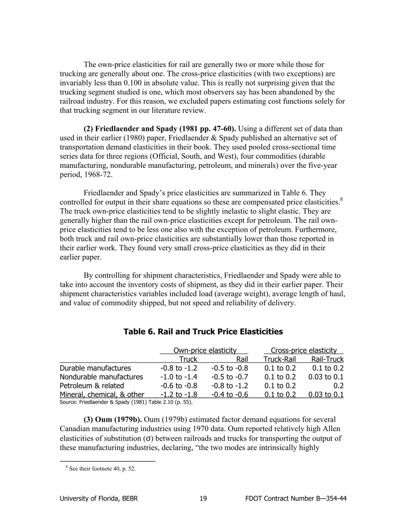
The own-price elasticities for rail are generally two or more while those for trucking are generally about one. The cross-price elasticities (with two exceptions) are invariably less than 0.100 in absolute value. This is really not surprising given that the trucking segment studied is one, which most observers say has been abandoned by the railroad industry. For this reason, we excluded papers estimating cost functions solely for that trucking segment in our literature review.
(2) Friedlaender and Spady (1981 pp. 47-60). Using a different set of data than
used in their earlier (1980) paper, Friedlaender & Spady published an alternative set of transportation demand elasticities in their book. They used pooled cross-sectional time series data for three regions (Official, South, and West), four commodities (durable manufacturing, nondurable manufacturing, petroleum, and minerals) over the five-year period, 1968-72.
Friedlaender and Spady’s price elasticities are summarized in Table 6. They
controlled for output in their share equations so these are compensated price elasticities.8 The truck own-price elasticities tend to be slightly inelastic to slight elastic. They are generally higher than the rail own-price elasticities except for petroleum. The rail own-price elasticities tend to be less one also with the exception of petroleum. Furthermore, both truck and rail own-price elasticities are substantially lower than those reported in their earlier work. They found very small cross-price elasticities as they did in their earlier paper.
By controlling for shipment characteristics, Friedlaender and Spady were able to
take into account the inventory costs of shipment, as they did in their earlier paper. Their shipment characteristics variables included load (average weight), average length of haul, and value of commodity shipped, but not speed and reliability of delivery.
Table 6. Rail and Truck Price Elasticities Own-price elasticity Cross-price elasticity Truck Rail Truck-Rail Rail-Truck Durable manufactures -0.8 to -1.2 -0.5 to -0.8 0.1 to 0.2 0.1 to 0.2 Nondurable manufactures -1.0 to -1.4 -0.5 to -0.7 0.1 to 0.2 0.03 to 0.1 Petroleum & related -0.6 to -0.8 -0.8 to -1.2 0.1 to 0.2 0.2 Mineral, chemical, & other -1.2 to -1.8 -0.4 to -0.6 0.1 to 0.2 0.03 to 0.1 Source: Friedlaender & Spady (1981) Table 2.10 (p. 55).
(3) Oum (1979b). Oum (1979b) estimated factor demand equations for several
Canadian manufacturing industries using 1970 data. Oum reported relatively high Allen elasticities of substitution (σ) between railroads and trucks for transporting the output of these manufacturing industries, declaring, “the two modes are intrinsically highly
8 See their footnote 40, p. 52.

University of Florida, BEBR FDOT Contract Number B—354-44 20
substitutable in moving most commodities, but less so for lumber.” (p. 476) He found much larger cross-price elasticities than Friedlaender and Spady (1980) found. On the other hand, Oum’s own-price elasticities were smaller than Friedlaender and Spady’s (1980) and were generally less than or equal to one. Oum did find (as did Friedlaender and Spady, 1980) that rail demand was usually more sensitive to its own price than truck demand was to its own price.
Table 7. Rail and Truck Price Elasticities and Elasticity of Substitution Own-price elasticity Cross-price elasticity Industry σ Rail Truck Truck-Rail Rail-Truck Fruits, vegetables, & edible foods 1.5 -1.0 -0.5 0.5 1.0 Lumber, including flooring 1.0 -0.5 -0.5 0.5 0.5 Chemicals 1.6 -0.6 -0.9 0.9 0.6 Fuel oil except gasoline 1.4 -0.4 -1.0 1.0 0.4 Refined petroleum products 1.4 -1.0 -0.4 0.4 1.0 Metallic products 1.5 -1.2 -0.3 0.3 1.2 Nonmetallic products 1.5 -1.0 -0.5 0.5 1.0 Source: Oum (1979b, Table 3).
Oum also published estimates of compensated elasticities of demand with respect
to speed (average transit time in days) and reliability (standard deviation of transit time). Demand is very inelastic with respect to the speed and reliability of railroads—all elasticities are less than or equal to 0.3—and often very elastic with respect to the speed and reliability of trucks. The cross elasticities of truck speed and reliability are higher than the own elasticities. Increasing the speed of trucks will not increase demand for trucks (elasticities range from 0.3 to 0.6) as much as reduce demand for railroads (elasticities range from -0.9 to -1.3).
Table 8. Rail and Truck Speed and Reliability Elasticities Speed Reliability Industry RR RT TR TT RR RT TR TT Fruits, vegetables, & edible foods 0.1 -0.9 -0.1 0.4 0.03 -2.4 -0.02 1.1 Metallic products 0 -1.1 0 0.3 0.2 -1.1 -0.05 0.3 Nonmetallic products 0.3 -1.3 -0.1 0.6 0.1 -2.5 -0.04 1.2 Source: Oum (1979b, Table 3). Elasticity of demand for Mode i with respect to speed (or reliability) of Mode j (R=railroad, T=truck).
(4) Morton (1969). Although this study predates Friedlaender and Spady’s (1981)
book we review it primarily because it is one of the few studies which estimated the elasticity of rail and truck freight with respect to Gross National Product (GNP), an elasticity we will use later in our analysis.
University of Florida, BEBR FDOT Contract Number B—354-44 21
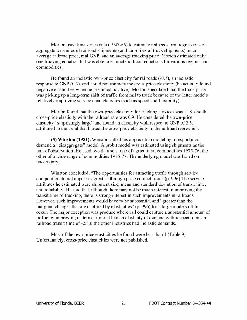
Morton used time series data (1947-66) to estimate reduced-form regressions of
aggregate ton-miles of railroad shipments (and ton-miles of truck shipments) on an average railroad price, real GNP, and an average trucking price. Morton estimated only one trucking equation but was able to estimate railroad equations for various regions and commodities.
He found an inelastic own-price elasticity for railroads (-0.7), an inelastic
response to GNP (0.3), and could not estimate the cross-price elasticity (he actually found negative elasticities when he predicted positive). Morton speculated that the truck price was picking up a long-term shift of traffic from rail to truck because of the latter mode’s relatively improving service characteristics (such as speed and flexibility).
Morton found that the own-price elasticity for trucking services was -1.8, and the
cross-price elasticity with the railroad rate was 0.9. He considered the own-price elasticity “surprisingly large” and found an elasticity with respect to GNP of 2.3, attributed to the trend that biased the cross price elasticity in the railroad regression.
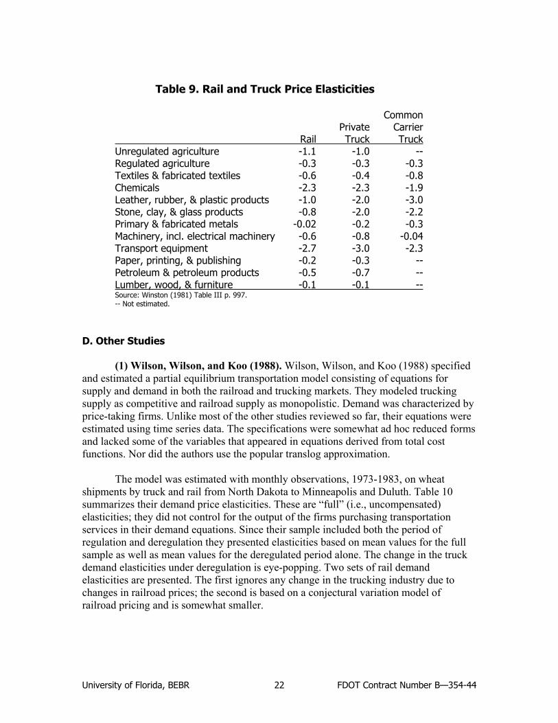
(5) Winston (1981). Winston called his approach to modeling transportation
demand a “disaggregate” model. A probit model was estimated using shipments as the unit of observation. He used two data sets, one of agricultural commodities 1975-76, the other of a wide range of commodities 1976-77. The underlying model was based on uncertainty.
Winston concluded, “The opportunities for attracting traffic through service
competition do not appear as great as through price competition.” (p. 996) The service attributes he estimated were shipment size, mean and standard deviation of transit time, and reliability. He said that although there may not be much interest in improving the transit time of trucking, there is strong interest in such improvements in railroads. However, such improvements would have to be substantial and “greater than the marginal changes that are captured by elasticities” (p. 996) for a large mode shift to occur. The major exception was produce where rail could capture a substantial amount of traffic by improving its transit time. It had an elasticity of demand with respect to mean railroad transit time of -2.33; the other industries had inelastic demands.
Most of the own-price elasticities he found were less than 1 (Table 9).
Unfortunately, cross-price elasticities were not published.
University of Florida, BEBR FDOT Contract Number B—354-44 22
Table 9. Rail and Truck Price Elasticities
Common Private Carrier Rail Truck Truck Unregulated agriculture -1.1 -1.0 -- Regulated agriculture -0.3 -0.3 -0.3 Textiles & fabricated textiles -0.6 -0.4 -0.8 Chemicals -2.3 -2.3 -1.9 Leather, rubber, & plastic products -1.0 -2.0 -3.0 Stone, clay, & glass products -0.8 -2.0 -2.2 Primary & fabricated metals -0.02 -0.2 -0.3 Machinery, incl. electrical machinery -0.6 -0.8 -0.04 Transport equipment -2.7 -3.0 -2.3 Paper, printing, & publishing -0.2 -0.3 -- Petroleum & petroleum products -0.5 -0.7 -- Lumber, wood, & furniture -0.1 -0.1 -- Source: Winston (1981) Table III p. 997. -- Not estimated.
D. Other Studies
(1) Wilson, Wilson, and Koo (1988). Wilson, Wilson, and Koo (1988) specified
and estimated a partial equilibrium transportation model consisting of equations for supply and demand in both the railroad and trucking markets. They modeled trucking supply as competitive and railroad supply as monopolistic. Demand was characterized by price-taking firms. Unlike most of the other studies reviewed so far, their equations were estimated using time series data. The specifications were somewhat ad hoc reduced forms and lacked some of the variables that appeared in equations derived from total cost functions. Nor did the authors use the popular translog approximation.
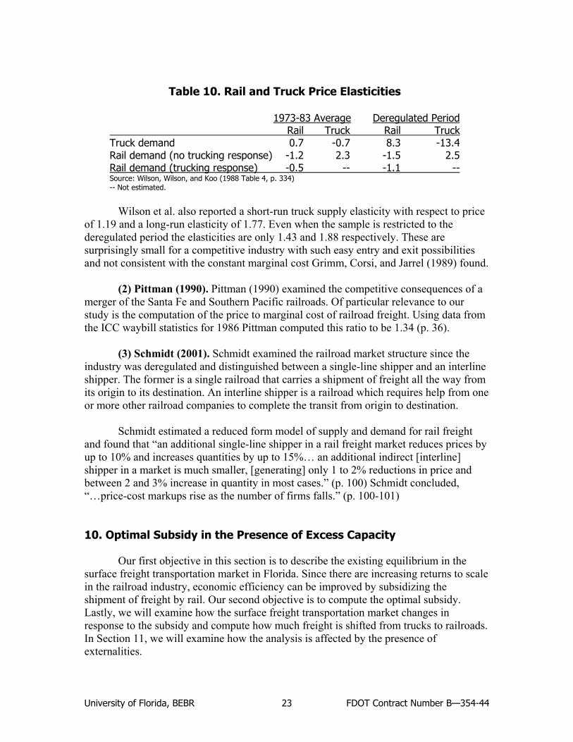
The model was estimated with monthly observations, 1973-1983, on wheat
shipments by truck and rail from North Dakota to Minneapolis and Duluth. Table 10 summarizes their demand price elasticities. These are “full” (i.e., uncompensated) elasticities; they did not control for the output of the firms purchasing transportation services in their demand equations. Since their sample included both the period of regulation and deregulation they presented elasticities based on mean values for the full sample as well as mean values for the deregulated period alone. The change in the truck demand elasticities under deregulation is eye-popping. Two sets of rail demand elasticities are presented. The first ignores any change in the trucking industry due to changes in railroad prices; the second is based on a conjectural variation model of railroad pricing and is somewhat smaller.
University of Florida, BEBR FDOT Contract Number B—354-44 23
Table 10. Rail and Truck Price Elasticities 1973-83 Average Deregulated Period Rail Truck Rail Truck Truck demand 0.7 -0.7 8.3 -13.4 Rail demand (no trucking response) -1.2 2.3 -1.5 2.5 Rail demand (trucking response) -0.5 -- -1.1 -- Source: Wilson, Wilson, and Koo (1988 Table 4, p. 334) -- Not estimated.
Wilson et al. also reported a short-run truck supply elasticity with respect to price
of 1.19 and a long-run elasticity of 1.77. Even when the sample is restricted to the deregulated period the elasticities are only 1.43 and 1.88 respectively. These are surprisingly small for a competitive industry with such easy entry and exit possibilities and not consistent with the constant marginal cost Grimm, Corsi, and Jarrel (1989) found.
(2) Pittman (1990). Pittman (1990) examined the competitive consequences of a
merger of the Santa Fe and Southern Pacific railroads. Of particular relevance to our study is the computation of the price to marginal cost of railroad freight. Using data from the ICC waybill statistics for 1986 Pittman computed this ratio to be 1.34 (p. 36).
(3) Schmidt (2001). Schmidt examined the railroad market structure since the
industry was deregulated and distinguished between a single-line shipper and an interline shipper. The former is a single railroad that carries a shipment of freight all the way from its origin to its destination. An interline shipper is a railroad which requires help from one or more other railroad companies to complete the transit from origin to destination.
Schmidt estimated a reduced form model of supply and demand for rail freight
and found that “an additional single-line shipper in a rail freight market reduces prices by up to 10% and increases quantities by up to 15%… an additional indirect [interline] shipper in a market is much smaller, [generating] only 1 to 2% reductions in price and between 2 and 3% increase in quantity in most cases.” (p. 100) Schmidt concluded, “…price-cost markups rise as the number of firms falls.” (p. 100-101)
10. Optimal Subsidy in the Presence of Excess Capacity Our first objective in this section is to describe the existing equilibrium in the
surface freight transportation market in Florida. Since there are increasing returns to scale in the railroad industry, economic efficiency can be improved by subsidizing the shipment of freight by rail. Our second objective is to compute the optimal subsidy. Lastly, we will examine how the surface freight transportation market changes in response to the subsidy and compute how much freight is shifted from trucks to railroads. In Section 11, we will examine how the analysis is affected by the presence of externalities.
University of Florida, BEBR FDOT Contract Number B—354-44 24
It is important to keep in mind the reason for these calculations. They are not
intended as definitive answers to questions about the desirability of subsidizing railroad freight. Rather, they are intended to provide some guidance about the relative importance of different factors and to provide some direction for future empirical research. That research should aim to reduce the plausible range of the parameters we identify as most important.
We built a simple model of the surface freight transportation markets. It consists
of two railroad demand functions, one for Florida and one for the rest of the country in which Florida’s railroad companies operate. It is necessary to consider the rest of the country because costs depend on total shipments, not just the shipments in the state of Florida. These demand functions have a log-linear form and hence, constant elasticities. Freight shipments depend on the price of shipment by railroad, the price of shipment by truck, and the level of gross state product. The elasticities are assumed to be the same in both regions. Similarly, the model has two truck demand functions, one for Florida and one for the rest of the country. These demand functions have the same variables that are in the railroad demand functions and the elasticities are the same in each region. We assume that the marginal cost of shipping by truck is constant but that the marginal cost of shipping by railroad falls as shipments increase. We assume that there are two railroads, they each have the same marginal cost functions, and they share the market equally. The marginal cost functions are log linear and the only independent variable is the amount shipped. Railroads are assumed to set prices equal to some constant multiple of marginal cost. This multiple is called the “markup rate.” Welfare change is approximated as one-half the product of the change in price and the change in shipments, summed over both transportation industries.9
The model treats the Florida railroad market as a duopoly. It may be objected that
since most shippers in Florida do not have a choice of whether to ship by CSX or Norfolk Southern—only one railroad serves their particular location—it might be better to describe railroads in Florida as monopolists. We believe that duopoly is a better description for the following reason. The competitiveness of the railroad industry depends on the number of railroads serving both the destination as well as the origin. Since more than 75% of rail shipments originating in Florida are carried long distances of 250 or more miles10 it is very likely that the bulk of these shipments are across the state’s borders. Therefore, the competitiveness of railroads in Florida cannot be assessed without reference to the structure of the industry outside the state. The consensus among academic studies of the market structure of U.S. railroads is that there is a duopoly in the East and a duopoly in the West.
9 Simulations were performed with Aremos 5.3.01. Command files to replicate the results are named in a footnote to
the table in which they appear and are available upon request. 10 1992 Commodity Flow Survey—Florida, Table 3.
University of Florida, BEBR FDOT Contract Number B—354-44 25
Interline shipments—shipments in which a railcar is picked up at the origin by one company and exchanged with another company which delivers it to the destination—are common in the railroad industry. For example, CSX may be the only railroad with track to the Deerhaven coal-fired electricity generating plant in Gainesville, Florida. However, so long as CSX is not the only railroad with track to all of the fields from which Deerhaven purchases coal, the rail rates on coal shipments will be less than the monopoly rate. At most, CSX would be in a position to charge a monopoly rate only along that part of the route to Deerhaven for which there is no alternative—and it may not even do so there. To be sure, this is a controversial matter on which economists have not yet reached agreement and a complete evaluation is beyond the scope of this study. Winston, Corsi, Grimm, and Evans (1990) examine the issue and is a useful guide to other studies.
Schmidt (2001) measured competition by separately counting the number of
single-line railroads serving a particular origin and destination, the number of railroads serving only the origin, and the number of railroads serving only the destination. A railroad was considered to service a location if it owned or leased track at that location, whether or not it actually shipped freight on that track. The case of 1 single-line firm, 0 origin-only firms, and 0 destination-only firms is the only case properly called monopoly. All other cases have some degree of competition. Schmidt (2001) found that increasing the number of any type of firm (single-line, origin-only, or destination-only) lowered the rates charged for railroad shipments as one would expect when competition increases.
Although most of the following analysis will assume a duopolistic competition in
Florida, we will also examine how the results are affected in the case of monopoly and in the case of three railroads.
Freight shipments by railroad in Florida in 1997 amounted to 19.822 billion ton-
miles while freight shipments by truck were 30.361 billion ton-miles as reported in the Commodity Flow Survey.11 According to Wilson (1999), railroad revenue per ton-mile averaged 2.40 cents in 1997. We will use this as the price of freight shipment. We will use 8.42 cents per ton-mile as the price of freight shipment by truck, the average private cost reported by Forkenbrock (1999).12 (Since the trucking market has constant returns to scale and is competitive, economic theory says that the price charged will equal average cost of providing the service.) We will treat these prices and quantities as the initial equilibrium in Florida’s surface freight transportation market.
11 These quantities represent only shipments originating in Florida and hence, underestimate total traffic. They count
all miles from the origin to the destination, including those miles traveled outside the state and hence, overestimate traffic that the state might want to subsidize.
12 On the one hand, Forkenbrock’s (1999) estimate is perhaps too low because it excludes the average fixed cost of buildings and rolling stock. On the other hand, it is perhaps too high to the extent that it includes the average variable costs associated with terminal and warehousing operations of the sectors of general freight transport which do not compete with railroads.
University of Florida, BEBR FDOT Contract Number B—354-44 26
Given these conditions, the optimal price and quantity is given by the intersection of the market demand curve and the industry supply curve. The optimal subsidy is the difference between the optimal price and the price railroads would charge for the optimal quantity. It turns out that the optimal subsidy as a percentage of the optimal price paid depends only on the markup rate.
Caves, Christensen, Tretheway and Windle (1985) provide, perhaps, the best
analysis of railroad costs. They estimated that the elasticity of railroad marginal costs with respect to freight shipment was -0.5. This elasticity strictly applies only to the mean of their sample. Since they used a translog cost function, the elasticity varies as output changes. It is also well known that it is dangerous to extrapolate results beyond the range of values used in estimating a regression. We will, nevertheless, do so here and elsewhere in the analysis and therefore, the conclusions must be treated as illustrative, not definitive. In order to determine how sensitive the results are to the assumptions, we will also consider alternative values of key parameters. For instance, we will examine how the optimal subsidy changes as the elasticity of marginal cost with respect to freight shipment varies from zero to -0.9.
By assuming that the markup rate, (i.e., the ratio of price to marginal cost) is 1.34
(as computed by Pittman, 1990, p. 36), it follows that the marginal cost associated with the price characterizing the initial railroad equilibrium is 1.79 cents per ton-mile.
For the trucking industry, we will assume constant returns to scale in accordance
with the findings of Grimm, Corsi, and Jarrell (1989). We assume that the price elasticity of demand for railroad transportation is about -
1.0 (this is consistent with some of the estimates in Oum, 1979b). In contrast, Friedlaender and Spady (1980) found high own-price elasticities of demand for railroad transportation, generally -2 or more while Friedlaender and Spady (1981) found estimates of less than -1.
The own- and cross-price elasticities of demand for trucking (-0.5 and 0.5,
respectively) come from the range estimated by Oum (1979b). The range of estimates published by other researchers is wide. Representative of the high end is -2 found by Winston (1981), representative of an intermediate value is -1.2 found by Friedlaender and Spady (1981).
We assume that the cross-price elasticity of demand for railroad services with
respect to the price of truck transportation is about 1.0. This is in the range found by Oum (1979b).
Florida Gross State Product (GSP) in 1997 amounted to $389 billion. We assume
that the other region served by Florida’s railroads had a GSP ten times larger. The elasticity of demand for railroad and truck shipments with respect to GSP is assumed to

University of Florida, BEBR FDOT Contract Number B—354-44 27
be 0.3 and 0.6 respectively. The railroad elasticity is from Morton (1969) whose truck elasticity, 2.3, appears to be biased by omitted variables and so we will simply assume that it is twice the railroad elasticity. Since our model assumes that demand for shipments is identical across regions, we will use the demand equations to solve for railroad and truck shipments in the other regions given prices and GSP.
These assumptions are summarized in Table 11.
Table 11. Assumptions Elasticity of marginal cost with respect to output -0.5 Price of freight shipment, railroads (cents per ton-mile) 2.40 Price of freight shipment, trucks (cents per ton-mile) 8.42 Markup rate, railroads 1.34 Railroad freight, Florida (billion ton-miles) 19.822 Truck freight, Florida (billion ton-miles) 30.361 Elasticity of demand for shipment by railroad -1.0 Elasticity of demand for shipment by truck with respect to rail price 0.5 Elasticity of demand for shipment by truck -0.5 Elasticity of demand for shipment by railroad with respect to truck price 1.0 Elasticity of demand for shipment by railroad with respect to GSP 0.3 Elasticity of demand for shipment by truck with respect to GSP 0.6 Welfare loss per dollar of tax revenue 0.25 Florida Gross State Product (billion $) 389.473 Other region Gross State Product (billion $) 3,894.73
Given the model and these assumptions, a subsidy of 0.57 cent per ton-mile
would drive the market to the competitive equilibrium. (This result, along with the other results of the Base Case, is presented in Table 12.) With this subsidy, the price charged by railroads would fall from 2.40 cents to 2.24 cents. Shippers would pay only 1.67 cents. The subsidy as a percentage of the price paid is therefore 34%. The subsidy would have a very large effect, increasing traffic on the railroad by 43% or by nearly 9 billion ton-miles. The trucking industry does not lose traffic equal to the gains of the railroad industry. Truck traffic falls by only 5.0 billion ton-miles or 16%.
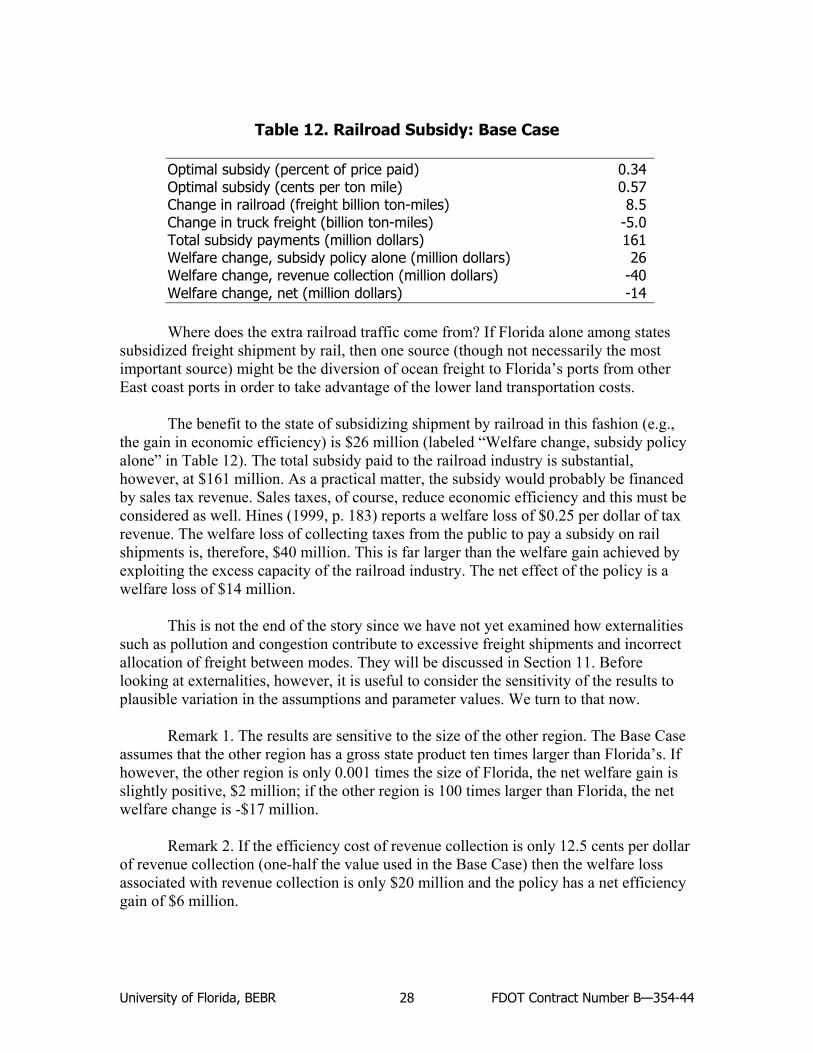
University of Florida, BEBR FDOT Contract Number B—354-44 28
Table 12. Railroad Subsidy: Base Case Optimal subsidy (percent of price paid) 0.34 Optimal subsidy (cents per ton mile) 0.57 Change in railroad (freight billion ton-miles) 8.5 Change in truck freight (billion ton-miles) -5.0 Total subsidy payments (million dollars) 161 Welfare change, subsidy policy alone (million dollars) 26 Welfare change, revenue collection (million dollars) -40 Welfare change, net (million dollars) -14
Where does the extra railroad traffic come from? If Florida alone among states
subsidized freight shipment by rail, then one source (though not necessarily the most important source) might be the diversion of ocean freight to Florida’s ports from other East coast ports in order to take advantage of the lower land transportation costs.
The benefit to the state of subsidizing shipment by railroad in this fashion (e.g.,
the gain in economic efficiency) is $26 million (labeled “Welfare change, subsidy policy alone” in Table 12). The total subsidy paid to the railroad industry is substantial, however, at $161 million. As a practical matter, the subsidy would probably be financed by sales tax revenue. Sales taxes, of course, reduce economic efficiency and this must be considered as well. Hines (1999, p. 183) reports a welfare loss of $0.25 per dollar of tax revenue. The welfare loss of collecting taxes from the public to pay a subsidy on rail shipments is, therefore, $40 million. This is far larger than the welfare gain achieved by exploiting the excess capacity of the railroad industry. The net effect of the policy is a welfare loss of $14 million.
This is not the end of the story since we have not yet examined how externalities
such as pollution and congestion contribute to excessive freight shipments and incorrect allocation of freight between modes. They will be discussed in Section 11. Before looking at externalities, however, it is useful to consider the sensitivity of the results to plausible variation in the assumptions and parameter values. We turn to that now.
Remark 1. The results are sensitive to the size of the other region. The Base Case
assumes that the other region has a gross state product ten times larger than Florida’s. If however, the other region is only 0.001 times the size of Florida, the net welfare gain is slightly positive, $2 million; if the other region is 100 times larger than Florida, the net welfare change is -$17 million.
Remark 2. If the efficiency cost of revenue collection is only 12.5 cents per dollar
of revenue collection (one-half the value used in the Base Case) then the welfare loss associated with revenue collection is only $20 million and the policy has a net efficiency gain of $6 million.
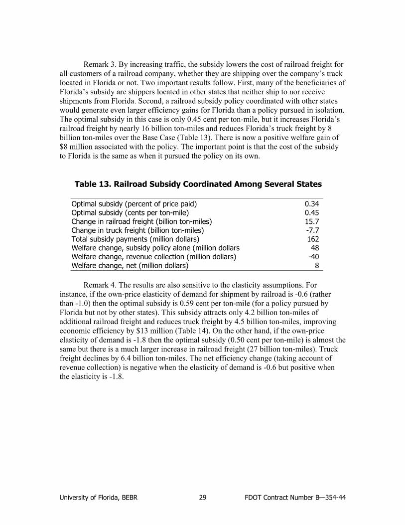
University of Florida, BEBR FDOT Contract Number B—354-44 29
Remark 3. By increasing traffic, the subsidy lowers the cost of railroad freight for all customers of a railroad company, whether they are shipping over the company’s track located in Florida or not. Two important results follow. First, many of the beneficiaries of Florida’s subsidy are shippers located in other states that neither ship to nor receive shipments from Florida. Second, a railroad subsidy policy coordinated with other states would generate even larger efficiency gains for Florida than a policy pursued in isolation. The optimal subsidy in this case is only 0.45 cent per ton-mile, but it increases Florida’s railroad freight by nearly 16 billion ton-miles and reduces Florida’s truck freight by 8 billion ton-miles over the Base Case (Table 13). There is now a positive welfare gain of $8 million associated with the policy. The important point is that the cost of the subsidy to Florida is the same as when it pursued the policy on its own.
Table 13. Railroad Subsidy Coordinated Among Several States Optimal subsidy (percent of price paid) 0.34 Optimal subsidy (cents per ton-mile) 0.45 Change in railroad freight (billion ton-miles) 15.7 Change in truck freight (billion ton-miles) -7.7 Total subsidy payments (million dollars) 162 Welfare change, subsidy policy alone (million dollars 48 Welfare change, revenue collection (million dollars) -40 Welfare change, net (million dollars) 8
Remark 4. The results are also sensitive to the elasticity assumptions. For
instance, if the own-price elasticity of demand for shipment by railroad is -0.6 (rather than -1.0) then the optimal subsidy is 0.59 cent per ton-mile (for a policy pursued by Florida but not by other states). This subsidy attracts only 4.2 billion ton-miles of additional railroad freight and reduces truck freight by 4.5 billion ton-miles, improving economic efficiency by $13 million (Table 14). On the other hand, if the own-price elasticity of demand is -1.8 then the optimal subsidy (0.50 cent per ton-mile) is almost the same but there is a much larger increase in railroad freight (27 billion ton-miles). Truck freight declines by 6.4 billion ton-miles. The net efficiency change (taking account of revenue collection) is negative when the elasticity of demand is -0.6 but positive when the elasticity is -1.8.
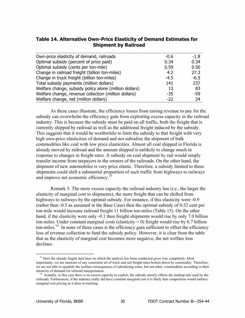
University of Florida, BEBR FDOT Contract Number B—354-44 30
Table 14. Alternative Own-Price Elasticity of Demand Estimates for Shipment by Railroad
Own-price elasticity of demand, railroads -0.6 -1.8 Optimal subsidy (percent of price paid) 0.34 0.34 Optimal subsidy (cents per ton-mile) 0.59 0.50 Change in railroad freight (billion ton-miles) 4.2 27.3 Change in truck freight (billion ton-miles) -4.5 -6.5 Total subsidy payments (million dollars) 141 237 Welfare change, subsidy policy alone (million dollars) 13 83 Welfare change, revenue collection (million dollars) -35 -59 Welfare change, net (million dollars) -22 24
As these cases illustrate, the efficiency losses from raising revenue to pay for the subsidy can overwhelm the efficiency gain from exploiting excess capacity in the railroad industry. This is because the subsidy must be paid on all traffic, both the freight that is currently shipped by railroad as well as the additional freight induced by the subsidy. This suggests that it would be worthwhile to limit the subsidy to that freight with very high own-price elasticities of demand and not subsidize the shipment of bulk commodities like coal with low price elasticities. Almost all coal shipped in Florida is already moved by railroad and the amount shipped is unlikely to change much in response to changes in freight rates. A subsidy on coal shipment by rail would simply transfer income from taxpayers to the owners of the railroads. On the other hand, the shipment of new automobiles is very price elastic. Therefore, a subsidy limited to these shipments could shift a substantial proportion of such traffic from highways to railways and improve net economic efficiency.13
Remark 5. The more excess capacity the railroad industry has (i.e., the larger the
elasticity of marginal cost to shipments), the more freight that can be shifted from highways to railways by the optimal subsidy. For instance, if this elasticity were -0.9 (rather than -0.5 as assumed in the Base Case) then the optimal subsidy of 0.52 cent per ton-mile would increase railroad freight 11 billion ton-miles (Table 15). On the other hand, if the elasticity were only -0.1 then freight shipments would rise by only 7.0 billion ton-miles. Under constant marginal costs (elasticity = 0) freight would rise by 6.7 billion ton-miles.14 In none of these cases is the efficiency gain sufficient to offset the efficiency loss of revenue collection to fund the subsidy policy. However, it is clear from the table that as the elasticity of marginal cost becomes more negative, the net welfare loss declines.
13 Here the already fragile data base on which the analysis has been conducted gives way completely. Most
importantly, we are unaware of any consistent set of truck and rail freight rates broken down by commodity. Therefore, we are not able to quantify the welfare consequences of subsidizing some, but not other, commodities according to their elasticity of demand for railroad transportation.
14 Actually, in this case there is no excess capacity to exploit; the subsidy merely offsets the markup rate used by the railroads. Furthermore, if the industry really did have constant marginal cost it is likely that competition would enforce marginal cost pricing as it does in trucking.
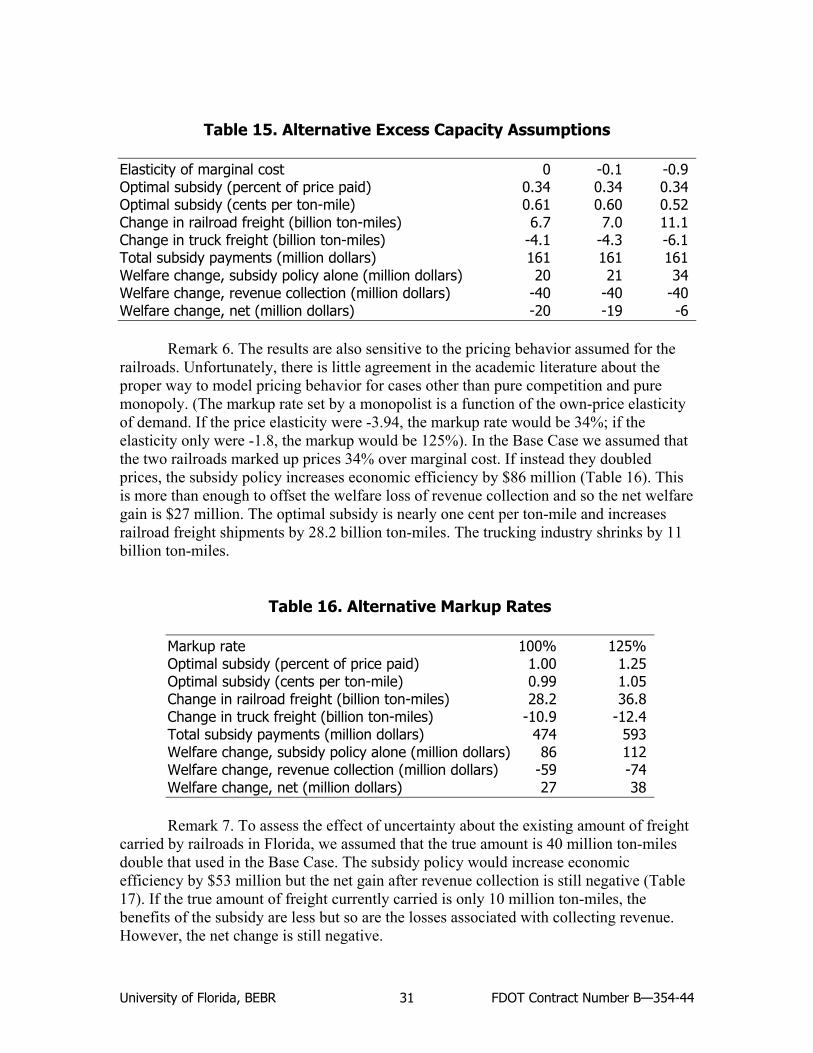
University of Florida, BEBR FDOT Contract Number B—354-44 31
Table 15. Alternative Excess Capacity Assumptions Elasticity of marginal cost 0 -0.1 -0.9 Optimal subsidy (percent of price paid) 0.34 0.34 0.34 Optimal subsidy (cents per ton-mile) 0.61 0.60 0.52 Change in railroad freight (billion ton-miles) 6.7 7.0 11.1 Change in truck freight (billion ton-miles) -4.1 -4.3 -6.1 Total subsidy payments (million dollars) 161 161 161 Welfare change, subsidy policy alone (million dollars) 20 21 34 Welfare change, revenue collection (million dollars) -40 -40 -40 Welfare change, net (million dollars) -20 -19 -6
Remark 6. The results are also sensitive to the pricing behavior assumed for the
railroads. Unfortunately, there is little agreement in the academic literature about the proper way to model pricing behavior for cases other than pure competition and pure monopoly. (The markup rate set by a monopolist is a function of the own-price elasticity of demand. If the price elasticity were -3.94, the markup rate would be 34%; if the elasticity only were -1.8, the markup would be 125%). In the Base Case we assumed that the two railroads marked up prices 34% over marginal cost. If instead they doubled prices, the subsidy policy increases economic efficiency by $86 million (Table 16). This is more than enough to offset the welfare loss of revenue collection and so the net welfare gain is $27 million. The optimal subsidy is nearly one cent per ton-mile and increases railroad freight shipments by 28.2 billion ton-miles. The trucking industry shrinks by 11 billion ton-miles.
Table 16. Alternative Markup Rates Markup rate 100% 125% Optimal subsidy (percent of price paid) 1.00 1.25 Optimal subsidy (cents per ton-mile) 0.99 1.05 Change in railroad freight (billion ton-miles) 28.2 36.8 Change in truck freight (billion ton-miles) -10.9 -12.4 Total subsidy payments (million dollars) 474 593 Welfare change, subsidy policy alone (million dollars) 86 112 Welfare change, revenue collection (million dollars) -59 -74 Welfare change, net (million dollars) 27 38 Remark 7. To assess the effect of uncertainty about the existing amount of freight
carried by railroads in Florida, we assumed that the true amount is 40 million ton-miles double that used in the Base Case. The subsidy policy would increase economic efficiency by $53 million but the net gain after revenue collection is still negative (Table 17). If the true amount of freight currently carried is only 10 million ton-miles, the benefits of the subsidy are less but so are the losses associated with collecting revenue. However, the net change is still negative.
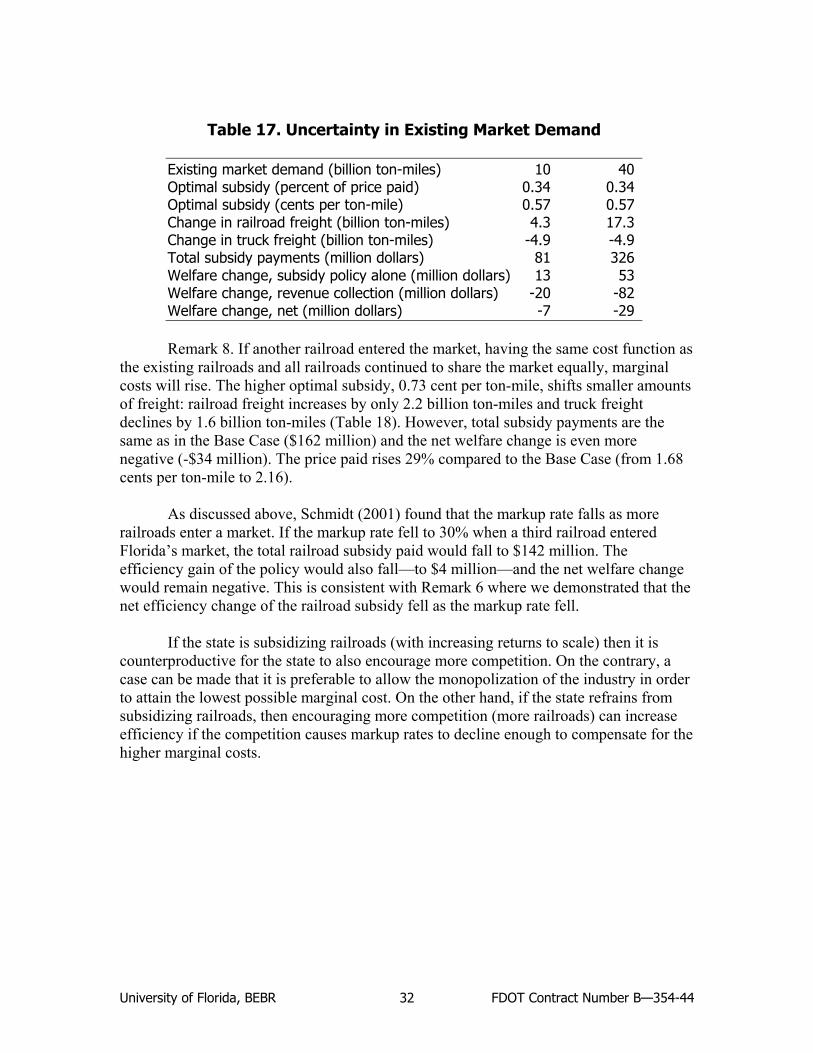
University of Florida, BEBR FDOT Contract Number B—354-44 32
Table 17. Uncertainty in Existing Market Demand Existing market demand (billion ton-miles) 10 40 Optimal subsidy (percent of price paid) 0.34 0.34 Optimal subsidy (cents per ton-mile) 0.57 0.57 Change in railroad freight (billion ton-miles) 4.3 17.3 Change in truck freight (billion ton-miles) -4.9 -4.9 Total subsidy payments (million dollars) 81 326 Welfare change, subsidy policy alone (million dollars) 13 53 Welfare change, revenue collection (million dollars) -20 -82 Welfare change, net (million dollars) -7 -29 Remark 8. If another railroad entered the market, having the same cost function as
the existing railroads and all railroads continued to share the market equally, marginal costs will rise. The higher optimal subsidy, 0.73 cent per ton-mile, shifts smaller amounts of freight: railroad freight increases by only 2.2 billion ton-miles and truck freight declines by 1.6 billion ton-miles (Table 18). However, total subsidy payments are the same as in the Base Case ($162 million) and the net welfare change is even more negative (-$34 million). The price paid rises 29% compared to the Base Case (from 1.68 cents per ton-mile to 2.16).
As discussed above, Schmidt (2001) found that the markup rate falls as more
railroads enter a market. If the markup rate fell to 30% when a third railroad entered Florida’s market, the total railroad subsidy paid would fall to $142 million. The efficiency gain of the policy would also fall—to $4 million—and the net welfare change would remain negative. This is consistent with Remark 6 where we demonstrated that the net efficiency change of the railroad subsidy fell as the markup rate fell.
If the state is subsidizing railroads (with increasing returns to scale) then it is
counterproductive for the state to also encourage more competition. On the contrary, a case can be made that it is preferable to allow the monopolization of the industry in order to attain the lowest possible marginal cost. On the other hand, if the state refrains from subsidizing railroads, then encouraging more competition (more railroads) can increase efficiency if the competition causes markup rates to decline enough to compensate for the higher marginal costs.
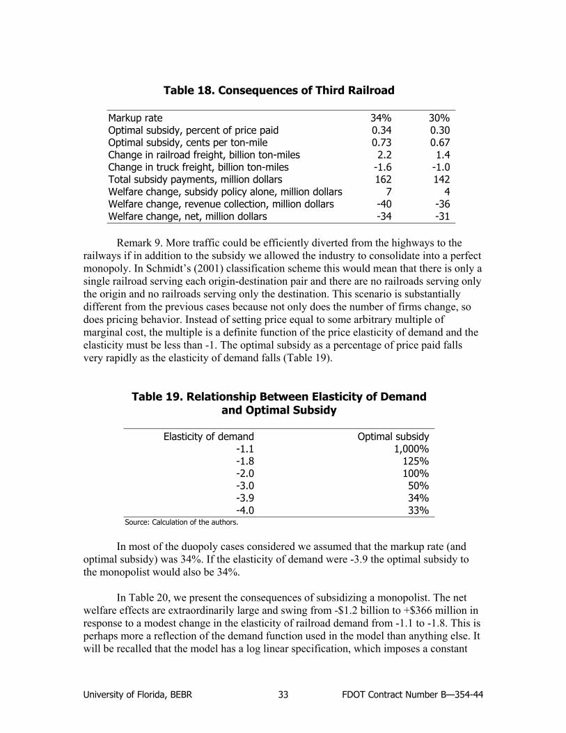
University of Florida, BEBR FDOT Contract Number B—354-44 33
Table 18. Consequences of Third Railroad Markup rate 34% 30% Optimal subsidy, percent of price paid 0.34 0.30 Optimal subsidy, cents per ton-mile 0.73 0.67 Change in railroad freight, billion ton-miles 2.2 1.4 Change in truck freight, billion ton-miles -1.6 -1.0 Total subsidy payments, million dollars 162 142 Welfare change, subsidy policy alone, million dollars 7 4 Welfare change, revenue collection, million dollars -40 -36 Welfare change, net, million dollars -34 -31
Remark 9. More traffic could be efficiently diverted from the highways to the
railways if in addition to the subsidy we allowed the industry to consolidate into a perfect monopoly. In Schmidt’s (2001) classification scheme this would mean that there is only a single railroad serving each origin-destination pair and there are no railroads serving only the origin and no railroads serving only the destination. This scenario is substantially different from the previous cases because not only does the number of firms change, so does pricing behavior. Instead of setting price equal to some arbitrary multiple of marginal cost, the multiple is a definite function of the price elasticity of demand and the elasticity must be less than -1. The optimal subsidy as a percentage of price paid falls very rapidly as the elasticity of demand falls (Table 19).
Table 19. Relationship Between Elasticity of Demand and Optimal Subsidy
Elasticity of demand Optimal subsidy -1.1 1,000% -1.8 125% -2.0 100% -3.0 50% -3.9 34% -4.0 33% Source: Calculation of the authors.
In most of the duopoly cases considered we assumed that the markup rate (and
optimal subsidy) was 34%. If the elasticity of demand were -3.9 the optimal subsidy to the monopolist would also be 34%.
In Table 20, we present the consequences of subsidizing a monopolist. The net
welfare effects are extraordinarily large and swing from -$1.2 billion to +$366 million in response to a modest change in the elasticity of railroad demand from -1.1 to -1.8. This is perhaps more a reflection of the demand function used in the model than anything else. It will be recalled that the model has a log linear specification, which imposes a constant
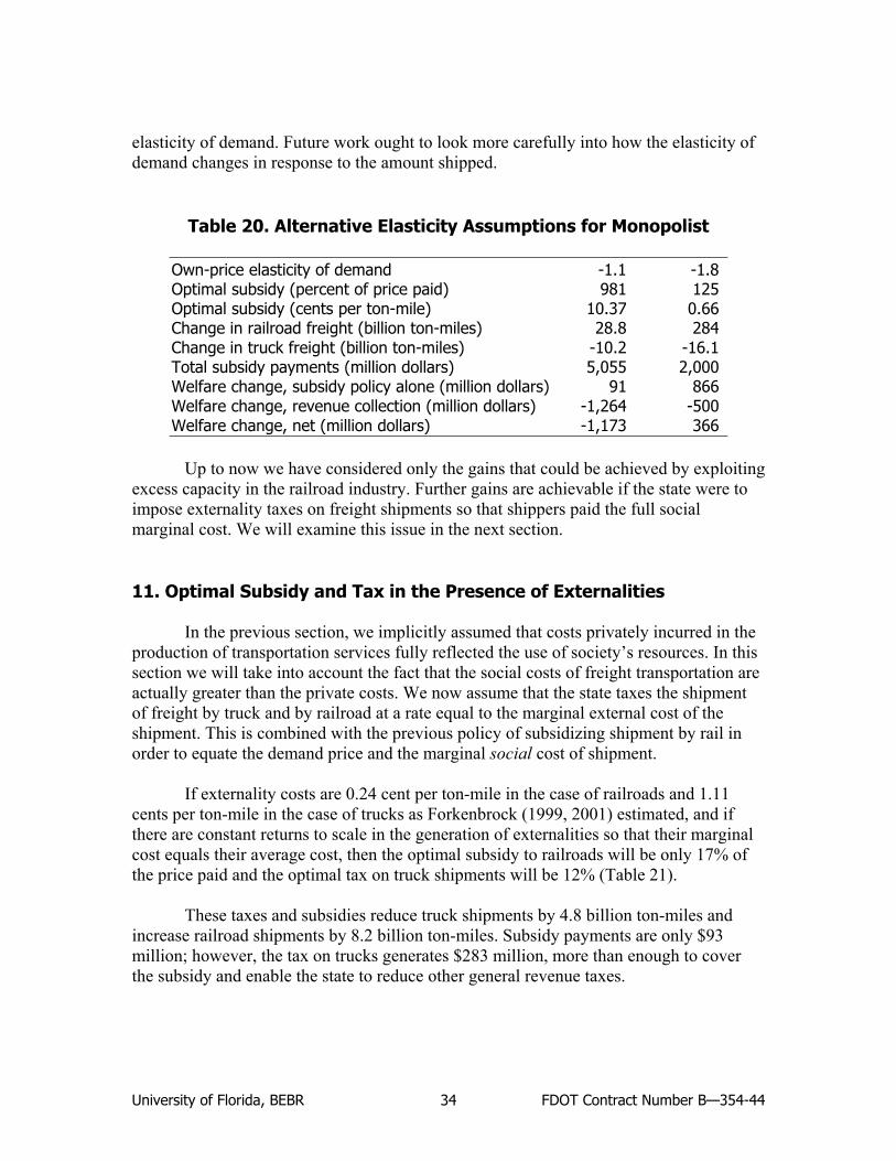
University of Florida, BEBR FDOT Contract Number B—354-44 34
elasticity of demand. Future work ought to look more carefully into how the elasticity of demand changes in response to the amount shipped.
Table 20. Alternative Elasticity Assumptions for Monopolist Own-price elasticity of demand -1.1 -1.8 Optimal subsidy (percent of price paid) 981 125 Optimal subsidy (cents per ton-mile) 10.37 0.66 Change in railroad freight (billion ton-miles) 28.8 284 Change in truck freight (billion ton-miles) -10.2 -16.1 Total subsidy payments (million dollars) 5,055 2,000 Welfare change, subsidy policy alone (million dollars) 91 866 Welfare change, revenue collection (million dollars) -1,264 -500 Welfare change, net (million dollars) -1,173 366
Up to now we have considered only the gains that could be achieved by exploiting
excess capacity in the railroad industry. Further gains are achievable if the state were to impose externality taxes on freight shipments so that shippers paid the full social marginal cost. We will examine this issue in the next section.
11. Optimal Subsidy and Tax in the Presence of Externalities In the previous section, we implicitly assumed that costs privately incurred in the
production of transportation services fully reflected the use of society’s resources. In this section we will take into account the fact that the social costs of freight transportation are actually greater than the private costs. We now assume that the state taxes the shipment of freight by truck and by railroad at a rate equal to the marginal external cost of the shipment. This is combined with the previous policy of subsidizing shipment by rail in order to equate the demand price and the marginal social cost of shipment.
If externality costs are 0.24 cent per ton-mile in the case of railroads and 1.11
cents per ton-mile in the case of trucks as Forkenbrock (1999, 2001) estimated, and if there are constant returns to scale in the generation of externalities so that their marginal cost equals their average cost, then the optimal subsidy to railroads will be only 17% of the price paid and the optimal tax on truck shipments will be 12% (Table 21).
These taxes and subsidies reduce truck shipments by 4.8 billion ton-miles and
increase railroad shipments by 8.2 billion ton-miles. Subsidy payments are only $93 million; however, the tax on trucks generates $283 million, more than enough to cover the subsidy and enable the state to reduce other general revenue taxes.

University of Florida, BEBR FDOT Contract Number B—354-44 35
This policy provides a net welfare gain to the state of $59 million. Surprisingly, the gain to the state of exploiting excess capacity in the railroad industry and forcing shippers to pay the social marginal cost of transportation is only $11 million. By far the largest part of the net welfare change, $48 million, comes from the reduction in general revenue collection made possible by the huge amount of externality taxes collected on shipments by truck.
The change in railroad and truck freight is not very sensitive to the size of the
externality. Cutting the externality in half or doubling it changes freight shipments of each mode by no more than 0.2 billion ton-miles. The size of the externality, however, does greatly affect the subsidy payments and the welfare change. If externalities are only one-half of Forkenbrock’s (1999, 2001) estimates, then the net welfare gain of the tax and subsidy policy is only $21 million. If externalities are actually twice as large as Forkenbrock’s (1999, 2001) estimates, then the net welfare gain is $138 million.
Table 21. Alternative Externality Estimates Railroad externality (cents per ton-mile) 0.12 0.24 0.48 Truck externality (cents per ton-mile) 0.56 1.11 2.22 Optimal subsidy, railroads (percent of price paid) 0.25 0.17 0.04 Optimal subsidy, railroads (cents per ton-mile) 0.45 0.33 0.09 Optimal tax, trucks (percent) 0.06 0.12 0.21 Optimal tax, trucks (cents per ton mile) 0.56 1.11 2.22 Change in railroad freight (billion ton-miles) 8.4 8.2 8.0 Change in truck freight (billion ton-miles) -4.9 -4.8 -4.7 Total subsidy payments (million dollars) 127 93 26 Cost of tax policy (million dollars) -141 -283 -569 Welfare change, subsidy policy alone (million dollars) 18 11 2 Welfare change, revenue collection (million dollars) 4 48 136 Welfare change, net (million dollars) 21 59 138
Remark 10. Externality taxes are vehemently opposed by the truck lobby and
currently appear to have little chance of being implemented. There is perhaps less opposition to the use of subsidies. In our final simulation (Table 22); the state optimizes a subsidy for rail shipment to exploit excess capacity but also takes into account externalities associated with railroads. Our efficiency calculations take into account the reduction in externalities when truck freight is shifted to railroads, but we do not tax the externalities associated with trucks. We compute the efficiency change as equal to one-half the product of the change in prices and quantities shipped in the railroad industry plus the product of the truck externality and the change in the amount shipped by truck.
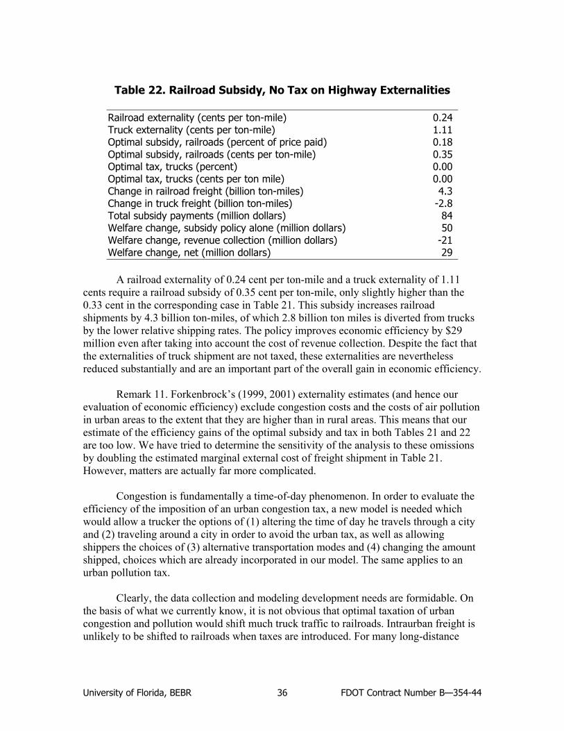
University of Florida, BEBR FDOT Contract Number B—354-44 36
Table 22. Railroad Subsidy, No Tax on Highway Externalities Railroad externality (cents per ton-mile) 0.24 Truck externality (cents per ton-mile) 1.11 Optimal subsidy, railroads (percent of price paid) 0.18 Optimal subsidy, railroads (cents per ton-mile) 0.35 Optimal tax, trucks (percent) 0.00 Optimal tax, trucks (cents per ton mile) 0.00 Change in railroad freight (billion ton-miles) 4.3 Change in truck freight (billion ton-miles) -2.8 Total subsidy payments (million dollars) 84 Welfare change, subsidy policy alone (million dollars) 50 Welfare change, revenue collection (million dollars) -21 Welfare change, net (million dollars) 29
A railroad externality of 0.24 cent per ton-mile and a truck externality of 1.11
cents require a railroad subsidy of 0.35 cent per ton-mile, only slightly higher than the 0.33 cent in the corresponding case in Table 21. This subsidy increases railroad shipments by 4.3 billion ton-miles, of which 2.8 billion ton miles is diverted from trucks by the lower relative shipping rates. The policy improves economic efficiency by $29 million even after taking into account the cost of revenue collection. Despite the fact that the externalities of truck shipment are not taxed, these externalities are nevertheless reduced substantially and are an important part of the overall gain in economic efficiency.
Remark 11. Forkenbrock’s (1999, 2001) externality estimates (and hence our
evaluation of economic efficiency) exclude congestion costs and the costs of air pollution in urban areas to the extent that they are higher than in rural areas. This means that our estimate of the efficiency gains of the optimal subsidy and tax in both Tables 21 and 22 are too low. We have tried to determine the sensitivity of the analysis to these omissions by doubling the estimated marginal external cost of freight shipment in Table 21. However, matters are actually far more complicated.
Congestion is fundamentally a time-of-day phenomenon. In order to evaluate the
efficiency of the imposition of an urban congestion tax, a new model is needed which would allow a trucker the options of (1) altering the time of day he travels through a city and (2) traveling around a city in order to avoid the urban tax, as well as allowing shippers the choices of (3) alternative transportation modes and (4) changing the amount shipped, choices which are already incorporated in our model. The same applies to an urban pollution tax.
Clearly, the data collection and modeling development needs are formidable. On
the basis of what we currently know, it is not obvious that optimal taxation of urban congestion and pollution would shift much truck traffic to railroads. Intraurban freight is unlikely to be shifted to railroads when taxes are introduced. For many long-distance

University of Florida, BEBR FDOT Contract Number B—354-44 37
shipments, the proportion of miles through urban areas is low so that even a very high per-mile urban tax might add little to the rate charged.
12. Extensions In our simulations we have ignored other general equilibrium aspects of the
problem. For instance, the model does not include a feedback from changes in the transportation markets (prices and amounts shipped) to Gross State Product. Nor does the model take into account the regional redistribution of production within the United States that might be induced by Florida’s rail subsidy.15
A subsidy which lowered transportation costs in Florida would make the state
more competitive in the national market place. For instance, shipments of vegetables from south Florida to other states would likely increase. As a consequence there would be less vegetable farming in say, New Jersey and more in Miami-Dade County. Second, in the longer run more firms may relocate to Florida to take advantage of the cheaper transportation costs. One can think usefully of the United States as a single market with plants distributed around the country. The level of operation of these plants changes as relative regional input prices change. It is possible that in addition to the increased railroad capacity utilization achieved by the subsidy, the size of the state’s economy would also be increased. A sufficiently large increase in GSP would increase truck traffic and reduce the initial improvement in congestion. However, this is unlikely. If Florida really could boost GSP substantially in this fashion, surely other states would respond with their own transportation subsidies.
The model is limited to the truck and railroad components of surface freight
transportation. Clearly, some aspects of the analysis will be affected by competition from pipelines, barges, and airlines. Just as clearly there is competition in the form of communications which also can be substituted for transportation in some situations (e.g., Internet delivery of news versus newspaper).
A policy of subsidizing freight shipment by railroad conflicts with the existing
policy of subsidizing passenger travel by rail in southeast Florida. As noted above, Kim (1987) estimated that the elasticity of the cost of freight shipment with respect to passenger travel and the elasticity of the cost of passenger travel with respect to freight shipment are both positive. Our model has not accounted for the increased cost of such passenger travel (state subsidies for a given amount of passenger travel by rail would rise) in south Florida as a consequence of subsidized rail freight shipment, but clearly it would reduce the net benefit of the railroad subsidy. However, if the findings of Kain
15 Although Friedlaender and Spady (1981) found that a 10% increase in rail and truck shipment rates (across all
regions) caused manufacturing employment declines ranging from as low as 0.1% to as high as 5.0%, they described the large impacts as “somewhat surprising” (p. 310). They also found that the reverse linkage (from changes in regional incomes to changes in freight rates) was not significant (pp. 73, 80, 103).

University of Florida, BEBR FDOT Contract Number B—354-44 38
(1999) are accepted, the better policy might be to reduce passenger travel by rail.16 A simple policy of shifting passenger transit subsidies from railroads to busses, for instance, would increase economic efficiency by itself as well as increase freight shipments by railroad and reduce freight shipments by truck—all at zero cost to the state. However, a full evaluation of this policy is beyond the scope of the current study.
13. Political Economy Considerations Even when a well designed subsidy program would create clear gains in economic
efficiency in the directly effected markets at the time the subsidy program is implemented, two additional factors must be considered in evaluating any subsidy program. First, the subsidy program might have dynamic consequences or consequences in indirectly effected markets that are not captured by static analysis of the directly impacted markets. Second, political considerations may cause the subsidy program to be implemented in a way that reduces or eliminates the potential economic gains. We briefly consider each of these possibilities.
Like any government interventions in markets, subsidy programs may have
unintended indirect consequences in related markets or in the subsidized market over time. As an example familiar to Florida, consider U.S. sugar policies.17 While less straightforward than a simple per unit subsidy, a combination of import quotas and loan programs are used to protect the domestic sugar industry. While keeping prices and/or output above competitive levels has resulted in large predictable social losses due to economic distortions, the sugar price supports clearly have had the intended impact of redistributing wealth to the sugar industry.18 However, they have also had other unintended and less easily predicted costs. By raising sugar prices sugar policy has also provided an impetus over time for users to develop methods of economizing on sugar or to move operations out of the U.S. to take advantage of much lower world sugar prices– clearly a distortion of resources from the social perspective. They have also had unintended indirect impacts upon environmental quality in the Florida Everglades by stimulating artificially high growth in the number of acres devoted to sugar cane production.19 The extent of such unanticipated impacts in the context of a rail freight subsidy program is of course unknown. One potential example would be a shift in Florida’s economic activity toward industries that are relatively larger users of rail. While we cannot enumerate and quantify such consequences before the fact, the possibility should not be totally disregarded.
16 “With few exceptions, academic studies of the cost-effectiveness of alternative modes of transportation have found
that some form of express bus system, operating on either an exclusive right-of-way or a shared congestion-free facility, would have lower costs and higher performance than either light or heavy rail systems in nearly all, if not all, U.S. cities.” Kain (1999, p. 384).
17 See Alvarez (1991) for a description of the sugar program history. 18 See USGAO (2000a). 19 Agricultural subsidies have created externalities in other crop industries. See Tolman (1995) and USGAO (2000b).
University of Florida, BEBR FDOT Contract Number B—354-44 39
Once a subsidy program is established, the ongoing level of the subsidy will be determined not strictly on grounds of economic efficiency, but also by political concerns. Potential beneficiary groups have an incentive to expend resources in an effort to capture benefits from the program. Similarly, groups who might be negatively impacted by the program (for instance, by bearing the cost of a subsidy) will have an incentive to invest resources to mitigate these negative impacts. Economists argue that time and other resources devoted to fighting over the division of benefits and costs from such a program are wasted from a social point of view and should properly be regarded as additional costs of government programs. Also, this political involvement means that the decision (in this case, the level of the subsidy) will diverge from the socially desirable level toward the level favored by the group with the most political strength.20 Intense lobbying by Archer Daniels Midland and various agriculture-based political action committees in support of more stringent ethanol requirements for reformulated gasoline, in spite of serious reservations about the net environmental benefits of ethanol use, is one recent example of this phenomenon.21
In the context of a rail freight subsidy, we might imagine that rail companies and
customers that are either heavy rail customers or have the potential to switch a lot of traffic to rail would lobby for higher subsidies, while the trucking industry and any group that might be harmed by a switch from truck to rail would lobby for lower subsidies or the elimination of the subsidies. If those who are harmed by such a program form the relatively stronger interest group, the program likely would not come to pass unless combined with a broader transportation policy that resulted in net gains to the stronger group, thus achieving “buy-in.” In this case, the program might become distorted to emphasize the aspects of the modified policy that benefited the truck lobby while leaving the freight subsidy under-funded. On the other hand, if those who would gain from the subsidy constituted the stronger group, the subsidy level might well end up higher than the social optimum. In either case, the full economic gains from an optimal subsidy program are unlikely to be realized since the actual subsidy will almost certainly diverge from the subsidy level that would best serve the general interest since it will exist in a political context.
Government intervention in the marketplace, even if ostensibly initiated with lofty
aims, can lead to unforeseen economic effects and to outcomes that favor politically strong groups rather than the general interest. These factors will mitigate any perceived benefits to the general welfare arising from the public policy. Therefore, it makes sense to initiate such intervention only when there are clear-cut and substantial economic benefits from the public policy in question. It also makes sense to try to choose policy mechanisms that, once in place, will be relatively insensitive to political pressure, at least in so far as possible. While our quantitative work indicated that there was certainly potential to capture significant economic gains by exploiting untapped rail freight
20 Tullock (1967 and 1980), Stigler (1971), Kruger (1974), Pozner (1975), Peltzman (1976), Becker (1983 and 1985), and Grossmand and Helpman (1994) represent important steps in the development of this line of political-economic theory. Ausin-Smith (1997) provides a useful survey of public choice models of interest group activity.
21 See, for example, Gardner (1995), Bovard (1995), and Moore (1997).
University of Florida, BEBR FDOT Contract Number B—354-44 40
capacity, it also indicated that a simple subsidy for rail freight shipments might have costs higher than benefits at this point. These political economy considerations constitute an additional argument that a rail freight subsidy is probably not a good idea at this time for Florida. Further, any other public policy choices intended to take advantage of Florida’s excess capacity for rail freight shipments should also weigh these factors carefully.
14. Summary and Policy Recommendations In this report we estimated the efficiency of subsidy and tax policies to correct the
market’s misallocation of freight shipment between the trucking and railroad industries. The partial equilibrium analysis of the efficiency gains of exploiting excess capacity in the railroad industry by a subsidy is the most complete; the analysis of the efficiency gains of taxing externalities associated with freight shipments by truck and by railroad is less complete and strictly applies to the intercity portion of the route. Before a comprehensive evaluation of the efficiency gains of taxing urban congestion and pollution can be performed, it will be necessary to develop better estimates of these costs and more sophisticated models to predict carrier route choice in the presence of taxes that vary spatially and temporally. Some of our main findings follow.
In all of the scenarios considered, subsidizing the shipment of freight by railroad reduced truck shipments—by as much as 16% in the Base Case. In some of the cases considered, we also reached the conclusion that subsidizing
the shipment of freight by rail improved economic efficiency by more than enough to offset the loss in efficiency caused by collecting the revenue to pay the subsidy. However, in many other cases we reached the opposite conclusion. The results of this analysis, therefore, are somewhat inconclusive: reasonable variation in key parameters can change net welfare from positive to negative. Further research is urgently needed to improve our estimates of the key parameters. However, the likelihood that a railroad subsidy will increase net social welfare is
higher if (1) externality taxes are charged, (2) Florida coordinates its subsidy with other states, and (3) the subsidy is limited to goods with very elastic own-price elasticities of demand for railroad shipment. On the other hand, subsidizing railroads conflicts with at least two other existing
public policies: subsidizing passenger travel on railroads and maintaining at least duopolistic competition in the railroad industry. Net social welfare can be enhanced perhaps by allowing a railroad monopoly and by removing subsidies to AMTRAK and commuter travel on railroads.

University of Florida, BEBR FDOT Contract Number B—354-44 41
Careful thought must be given to the value of the reduction in congestion that might be attained by the railroad subsidy. Taxes and subsidies on freight alone, ignoring automobiles, might be foolish if the reduction in congestion caused by trucks is offset by an increase in congestion caused by autos according to Down’s Law. In effect, the state would be subsidizing at great cost the use of highways by marginal car drivers. Even though a direct subsidy does not appear desirable at this time, public policy
should not ignore the potential to eventually exploit the excess capacity in Florida’s rail freight market. As Florida’s population continues to grow in coming decades, rail demand in Florida will increase due to two factors. First, the simple increase in the number of customers and firms in the state will cause demand for both truck and rail transport to grow. Second, population growth will likely outpace growth in highway infrastructure. Florida’s population is projected to grow from 16 million in 2000 to 21.7 million in 2020. If lane mileage grows according to its trend over the past 20 years, lane miles per 1,000 residents will fall from 15.9 to 13.8 over that period. Additional highway congestion will increase the costs of shipment by truck relative to the cost of shipment by rail since there is excess capacity in the rail freight market. Thus, existing excess capacity in Florida’s rail freight industry will naturally be put to use to provide some relief to the highway system as congestion worsens.
In order for this to happen, however, the rail network, particularly right of way,
must be maintained. While it may be tempting to divert right of way that is currently underutilized to other purposes, it is exceedingly difficult to reassemble right of way once it is lost. Even rails-to-trails projects raise this concern. Rails-to-trails projects—of which there are currently 420 miles in Florida according to the Rails-to-Trails Conservancy—do maintain large portions of abandoned corridors intact.22 However, these projects also create another class of user of the right of way who may be resistant to converting the right of way back to rail use in the future. Such a program is, however, preferable to outright loss of the right of way through conversion to uses that would not maintain the corridor intact. While it remains to future research to determine exactly what would constitute an optimal system preservation policy, this research strongly indicates that the potential efficiency gains from preserving and eventually exploiting the capacity of Florida’s rail system for freight movement is likely to be large.
In summary, for values of key parameters within the range that existing economic
research has indicated to be reasonable, our quantitative analysis revealed that a rail freight subsidy might have either positive or negative consequences for economic efficiency under current conditions. Together with the possibilities that a rail freight subsidy program might have unintended consequences beyond the scope of our model or become distorted by political pressure, these findings indicate that such a subsidy program does not seem advisable at this time. However, at some point in the future a subsidy program might be justified. This would require additional research that would
22 Rails-to-Trails Conservancy (2002).
University of Florida, BEBR FDOT Contract Number B—354-44 42
allow targeting of high elasticity market segments, coordination with other states, and implementation with other policies to manage peak travel demand on urban roads. Further, the potential for eventually exploiting the excess capacity in Florida’s rail freight market to address growing transportation needs means that Florida should carefully consider policies to preserve rail infrastructure, particularly in-tact right of way that now may appear economically unviable due to current underutilization.
University of Florida, BEBR FDOT Contract Number B—354-44 43
References
Alvarez, J. (1991). Sugar Policy series. Retrieved April 2002, from University of Florida, Institute for Food and Agricultural Sciences, Florida Cooperative Extension, Electronic Data Information Source Website, http://edis,ifas,ufl.edu/MENU_SC_POLICY.
Austin-Smith, D. (1997). Interest groups: Money, information and influence. In D.C.
Mueller (Ed.), Perspectives on Public Choice: A Handbook. Cambridge: Cambridge University Press.
Becker, G. (1983). A theory of competition among pressure groups for political
influence. Quarterly Journal of Economics, 98, 371-401. Becker, G. (1985). Public policies, pressure groups, and dead weight costs.” Journal of
Public Economics, 28(3), 329-347. Bovard, J. (1995). Archer Daniels Midland: A case study in corporate welfare. Cato
Policy Analysis No. 241. Boyer, K. D. (1977). Minimum rate regulation, modal split sensitivities, and the railroad
problem. Journal of Political Economy, 85, 493-512. Boyer, K. D. (1997). American trucking, NAFTA, and the cost of distance. The Annals of
the American Academy of Political and Social Science, 553, 55-65. Caves, D. W., Christensen, L. R., Tretheway, M. W., and Windle, R. J. (1985). Network
effects and the measurement of returns to scale and density for U. S. railroads. In A. F. Daughety (Ed.), Analytical studies in transport economics (pp. 97-120). New York: Cambridge University Press.
Christensen, L. R. and Huston, J. H. (1987). A reexamination of the cost structure for
specialized motor carriers. Logistics and Transportation Review, 23, 339-351. Committee for Study of Public Policy for Surface Freight Transportation. (1996). Paying
our way: Estimating marginal social costs of freight transportation (Transportation Research Board Special Report 246). Washington, DC: Transportation Research Board.
Forkenbrock, D. J. (1999). External costs of intercity truck freight transportation.
Transportation Research (Part A), 33, 505-526. Forkenbrock, D. J. (2001). Comparison of external costs of rail and truck freight
transportation. Transportation Research (Part A), 35, 321-337. Friedlaender, A. F. and Spady, R. H. (1980). A derived demand function for freight
transportation. The Review of Economics and Statistics, 62, 432-441. Friedlaender, A. F. and Spady, R. H. (1981). Freight transport regulation: Equity,
efficiency, and competition in the rail and trucking industries. Cambridge: The MIT Press.
University of Florida, BEBR FDOT Contract Number B—354-44 44
Gardner, B. D. (1995). Plowing ground in Washington. Pacific Research Institute for Public Policy. San Francisco, CA.
Grimm, C. M., Corsi, T. M., and Jarrell, J. L. (1989). U. S. motor carrier cost structure
under deregulation. Logistics and Transportation Review, 25, 231-249. Grossman, G. M., and Helpman, E. (1994). Protection for sale. The American Economic
Review, 84, 833-850. Harberger, A. (1954). Monopoly and resource allocation. The American Economic
Review, 44, 77-87. Hines, Jr., J. R. (1999). Three sides of Harberger Triangles. Journal of Economic
Perspectives, 13, 167-188. Ivaldi, M. and McCullough, G. J. (2001). Density and integration effects on Class I U. S.
freight railroads. Journal of Regulatory Economics, 19, 161-182. Kain, J. F. (1999). The urban transportation problem: A reexamination and update. In
José A. Gómez-Ibáñez and William B. Tye, (Eds.), Essays in transportation economics and policy: A handbook in honor of John R. Meyer. Washington, DC: The Brookings Institution.
Kim, H. Y. (1987). Economies of scale and scope in multiproduct firms: Evidence from
U. S. railroads. Applied Economics, 19, 733-741. Krueger, A. O. (1974). The political economy of the rent seeking society. American
Economic Review, 64, 291-303. Levin, R. C. (1978). Allocation in surface freight transportation: Does rate regulation
matter? The Bell Journal of Economics, 9, 18-45. Levin, R. C. (1981). Railroad rates, profitability, and welfare under deregulation. The
Bell Journal of Economics, 12, 1-26. Moore, S. (1997). Push ethanol off the Dole. Retrieved April 2002, from
http://www.cato.org/dailys/7-10-97.html. Morton, A. L. (1969). A statistical sketch of intercity freight demand. Highway Research
Record, (No. 296). Morton, A. L. (1972). Intermodal competition for the intercity transport of manufactures.
Land Economic, 48, 357-366. Olson, M. (1965). The logic of collective action. Cambridge, MA: Harvard Press. Oum, T. H. (1979a). A warning on the use of linear logit models in transport mode choice
studies. The Bell Journal of Economics, 10, 374-388.
University of Florida, BEBR FDOT Contract Number B—354-44 45
Oum, T. H. (1979b). A cross sectional study of freight transport demand and rail-truck competition in Canada. The Bell Journal of Economics, 10, 463-482.
Oum, T. H, Waters, II, W. G., and Yong, J. (1992). Concepts of price elasticities of
transport demand and recent empirical estimates: An interpretive survey. Journal of Transport Economics and Policy, 26, 139-154.
Peltzman, S. (1976). Toward a more general theory of regulation. Journal of Law and
Economics, 19(2), 211-240. Pittman, R. W. (1990). Railroads and competition: The Santa Fe/Southern Pacific merger
proposal. The Journal of Industrial Economics, 39, 25-46. Posner, R. A. (1975). The social costs of monopoly and regulation. Journal of Political
Economy, 83, 807-827. Rails-to-Trails Conservancy. Florida trail statistics. Retrieved September 2002, from
http://www.railtrails.org/field/florida/default.asp. Schmidt, S. (2001). Market structure and market outcomes in deregulated rail freight
markets. International Journal of Industrial Organization, 19, 99-131. Schrank, D. and Lomax, T. (2001). The 2001 urban mobility report. Retrieved from
Texas A & M University System, Texas Transportation Institute website: http://mobility.tamu.edu.
Small, K. A. and Winston, C. (1999). The demand for transportation: Models and
applications. In José A. Gómez-Ibáñez and William B. Tye (Eds.), Essays in transportation economics and policy: A handbook in honor of John R. Meyer (pp. 11-55). Washington, DC: The Brookings Institution.
Stigler, G. J. (1971). The economic theory of regulation. Bell Journal of Economics, 2, 3-
21. Tolman, J. (1995). Federal agricultural policy: A harvest of environmental abuse.
Competitive Enterprise Institute. Tullock, G. (1967). The welfare costs of tariffs, monopolies, and theft. Western Economic
Journal, 5, 224-232. Tullock, G. (1980). Efficient rent seeking. In J. M. Buchanan, R. D. Tollison, and G.
Tullock (Eds.), Toward a theory of the rent seeking society. College Station: Texas A&M University Press.
U. S. General Accounting Office. (2000b). Comprehensive Everglades restoration plan:
Additional water quality projects may be needed and could increase costs. GAO/T-RCED-00-297.
University of Florida, BEBR FDOT Contract Number B—354-44 46
U. S. General Accounting Office. (2000a). Sugar program: Supporting sugar prices has increased users’ costs while benefiting producers. GAO/RCED-00-126.
Wilson, R. A. (1999). Transportation in America. (17th Edition). Washington, DC: Eno
Transportation Foundation, Inc. Wilson, William W., Wilson, Wesley W., and Koo, W. W. (1988). Modal competition in
grain transport. Journal of Transport Economics and Policy, 22, 319-337. Winston, C. (1981). The welfare effects of ICC rate regulation revisited. The Bell Journal
of Economics, 12, 232-244. Winston, C., Corsi, T. M., Grimm, C. M., and Evans, C. A. (1990). The economic effects
of surface freight deregulation. Washington, DC: The Brookings Institution.