HAL Id: hal-01144547https://hal.inria.fr/hal-01144547

Submitted on 26 May 2015

HAL is a multi-disciplinary open accessarchive for the deposit and dissemination of sci-entific research documents, whether they are pub-lished or not. The documents may come fromteaching and research institutions in France orabroad, or from public or private research centers.

L’archive ouverte pluridisciplinaire HAL, estdestinée au dépôt et à la diffusion de documentsscientifiques de niveau recherche, publiés ou non,émanant des établissements d’enseignement et derecherche français ou étrangers, des laboratoirespublics ou privés.

The Replacement Bootstrap for Dependent DataAmir Sani, Alessandro Lazaric, Daniil Ryabko

To cite this version:Amir Sani, Alessandro Lazaric, Daniil Ryabko. The Replacement Bootstrap for Dependent Data.Proceedings of the IEEE International Symposium on Information Theory, Jun 2015, Hong Kong,Hong Kong SAR China. 2015. <hal-01144547>

The Replacement Bootstrap for Dependent DataAmir Sani

INRIA Lille, FranceAlessandro LazaricINRIA Lille, France

Daniil RyabkoINRIA Lille, France

Abstract—Applications that deal with time-series data oftenrequire evaluating complex statistics for which each time seriesis essentially one data point. When only a few time series areavailable, bootstrap methods are used to generate additionalsamples that can be used to evaluate empirically the statisticof interest. In this work a novel bootstrap method is proposed,which is shown to have some asymptotic consistency guaranteesunder the only assumption that the time series are stationary andergodic. This contrasts previously available results that imposemixing or finite-memory assumptions on the data. Empiricalevaluation on simulated and real data, using a practically relevantand complex extrema statistic is provided.

I. INTRODUCTION

A wide variety of applications, notably in economics, biol-ogy and environmental sciences, require estimating complexstatistics of highly dependent time-series distributions. Inmany cases, only a single data sequence generated by theunderlying process is available. In the case of dependenttime series, such a sequence is essentially one realization(or data point) w.r.t. the computation of a statistic of in-terest. Meaningful estimates are only possible when severaldata points are available, and these have to be somehowobtained from the single one given. For some statistics, simpleheuristics like chopping the available time series into manymay suffice, while for others they clearly do not. Practicallymeaningful examples of the latter situation include extrema-based statistics, such as maximum drawdown (the differencebetween the maximum and the minimum attained after it),or even more complex ones such as the performance of atrading algorithm on the given data. Estimating such statisticsrequire having multiple time series of length close to the timeseries of interest. There are, thus, three problems in estimatingsuch statistics: complex statistics, which appear impossible toanalyse theoretically, highly-dependent time series, and, as aconsequence of the latter, too few, or just a single sample.

Bootstrap methods attempt to tackle the latter problem bygenerating new samples from the available ones, in such away that these new samples are “likely” to be generated bythe underlying process distribution. The original Bootstrap [3]was designed for independent and identically distributed (i.i.d.)data; it samples with replacement from the original sequenceattempting to improve upon the estimates of simple statisticssuch as smooth functions of the mean [5, 23]. While gener-alizations to dependent data are available (some of these arebriefly reviewed below), they concern only rather restrictedclasses of processes, such as Markov chains or geometricallymixing time series. In general, even for simple statistics thetraditional bootstrap is concerned with, obtaining convergence

guarantees is highly problematic, and the available theoreticalresults all require additional assumptions on the distributions.Specifically, under assumptions such as moment conditionsand several conditions necessary for Edgeworth expansions,the i.i.d. Bootstrap, is a consistent estimator of the samplingdistribution for some specific statistics and it is shown toproduce asymptotic refinements for problems such as biasreduction and the construction of confidence intervals [5, 23].

In this paper we address the second problem (highly depen-dent time series), namely, we propose a bootstrap method fortime series which have performance guarantees under the onlyassumption that the time series are stationary ergodic. This isvastly more general than the assumptions made in prior works.However, we do not attempt to solve the problem of theoreticalanalysis of complex statistics; since no theoretical results forsuch complex statistics as we consider (max drawdown) areavailable even for the i.i.d. case, there is at present no hopefor dependent time series. Thus, the theoretical results wepresent establish the consistency of the proposed method forgenerating new time-series, and the performance in estimatingthe statistic of interest is evaluated empirically.

What we propose here is a novel, principally different,approach to generating bootstrap sequences, namely the re-placement bootstrap (RB). Bootstrap sequences are generatedby replacing elements in the original sequence according totheir estimated conditional probability distribution (replace-ment distribution) over the observed sequence around theirposition. First, R positions in the original sequence are se-lected at random. Next, the estimated conditional distributionat the selected positions is calculated using the full time seriesaround them. Finally, existing elements in these R positionsare replaced with elements drawn from each of the R estimatedreplacement distributions. The main idea is that, unlike in thei.i.d. or Markov cases, in highly-dependent time series it isimpossible to estimate the distribution of the whole sequence.It is, however, possible to estimate conditional distributionof a symbol given its past and future. Thus, instead ofgenerating whole new sequences from scratch, we start withthe one available and introduce some changes according toestimated replacement distributions, which we can expect tobe reliable. To estimate the replacement distribution, here weuse an estimator based on the universal measure R proposedin [17] (see also [18]). For this estimator we obtain theoreticalconsistency guarantees that hold for arbitrary stationary er-godic distributions, without relying on finite-memory, mixingor any other assumptions. Further, we study empirically theaccuracy of the proposed method on an extrema statistic (max

drawdown) that has been shown to be inconsistent in thetraditional bootstrap approaches. Additional details and resultsare reported in the extended version of this paper [21].

An important difference between the traditional applicationsof bootstrap and the one considered in this work should bepointed out. Typically, in the literature on bootstrap, one is in-terested in a statistic θ(P ) which concerns single-dimensionalmarginals of P . For i.i.d. data, these define the distributioncompletely. In more general cases, one is interested in esti-mating a statistic of k-dimensional marginals, where k � n.The intuition is that these should provide sufficient precisionfor estimating the distribution P or indeed any statistic thereof,such in the case of m-order Markov (where one can takek = m + 1) or mixing processes. However, in our casewe are interested in complex statistics θn(P ) concerning n-dimensional marginals, where n is the size of the sampleavailable, such as the performance of a (trading, learning, etc.)algorithm or the max drawdown. For stationary ergodic timeseries, studying these statistics cannot be reduced to studyingk-dimensional distributions and thus the object of our study isnot exactly the same as in traditional applications of bootstrap.Prior work. Universal measures, such as R and those basedon data compressors, are used for solving various statisticalproblems concerning time series, often not directly relatedto prediction or compression [20, 18], but have not beenpreviously used for bootstrap. Next we briefly review twopopular model free Bootstrap approaches to dependent data:block based methods and methods that rely on the Markovproperty (for a comprehensive review, see, e.g., [8]). Blockmethods are a direct generalization of the i.i.d. bootstrap todependent data. Block methods resample contiguous blocksof data from the original sequence to capture the dependencestructure defined by a block width. Block width selectiondetermines the bias-variance trade-off: small blocks increasebias, while larger blocks increase variance. As their perfor-mance relies on proper width selection, automatically selectionmethods have been introduced [15]. For relative performanceover various construction methods, see [11, 13]. Note that suchmethods necessarily ignore and break long-range dependencein the sequence. Therefore they are only suitable for processeswhere it is negligible, e.g., processes with fast mixing. Whenthe Markov property and regularity conditions are met, theMarkov bootstrap (MB) of [10] has been shown to be moreaccurate than block methods [7]. MB sequences are generatedby directly estimating a Markov model of a given order fromthe observed sequence, and then sampling from the model togenerate a bootstrap sequence. If the process generating thesequence is not Markov (or is Markov of a higher order) thenthe MB may perform worse than block-based methods.

II. PRELIMINARIES

A sequence Xn = (X1, . . . , Xn) is generated by a time-series distribution P over a finite alphabet A. We introduce thenotation X<t = (X1, . . . , Xt−1), X>t = (Xt+1, . . . , Xn),and Xt:t′ = (Xt, . . . , Xt′) and we denote νXn

(a1, . . . , am)=

#{s ≤ n : Xs = am, . . . , Xs−m+1 = a1} the number ofoccurrences of a word (a1, . . . , am) in Xn. We assume that:

Assumption 1. The process P is stationary, i.e. for any m,τ ∈ N , and any word vm = (a1, . . . , am) ∈ Am

P (X1=a1, . . . , Xm=am)=P (X1+τ =a1, . . . , Xm+τ =am),

and ergodic, i.e., for any word vm = (a1, . . . , am) thefrequency of vm in a sequence Xn tends to its probability a.s.:P (νXn(a1, . . . , am)/n→ P (X1 = a1, . . . , Xm = am)) = 1.

(The latter definition of ergodicity is equivalent to the usualone involving shift-invariant sets [4].) This assumption isvastly more general than those used in the literature onnonparametric (model free) bootstrap methods for time series,and allows us to focus on what is arguably the most generalclass of processes for which it is still possible to define mean-ingful statistical inference problems. We recall the definitionof the Kullback-Leibler (KL) divergence, used to measure theaccuracy of estimated distributions. Given two distributions Pand Q over A, the KL divergence between P and Q is

KL(P ;Q) =∑a∈A

P (a) log(P (a)/Q(a)). (1)

We use h for the Shannon entropy, hk(P ) for the kth orderentropy of the distribution P , and h∞(P ) for its entropy rate.

A bootstrap algorithm is a random mapping Bn : An An,such that given Xn, Bn(Xn) returns a (random) bootstrapsequence bn of length n. The intuition behind the bootstrapapproach is that a sequence Xn might provide enough infor-mation about P to generate additional sequences which arelikely to be generated by P . Thus, given a single sequenceXn, a bootstrap algorithm Bn repeatedly generates bootstrapsequences b1n, . . . , b

Bn . These sequence, together with the

original Xn are then used to estimated the statistic of interest.

III. THE REPLACEMENT BOOTSTRAP

The main idea of the replacement bootstrap (RB) is tochoose a set of R random positions 1 ≤ t1, . . . , tR ≤ n in theoriginal sequence Xn and replace symbols (Xt1 , . . . , XtR)with symbols (bt1 , . . . , btR), drawn from the distributionP (a1, . . . , aR|Xn − {Xt1 , Xt2 , . . . , XtR}), where P is anestimation of the distribution P generating the data. The RBpreserves part of the original sequence’s temporal structure,while simultaneously exploiting the full sequence to determinereplacements through an estimate of the conditional distribu-tion P (a1, . . . , aR|Xn−{Xt1 , Xt2 , . . . , XtR}). It is importantto note that the estimated distribution is conditional both onthe past and the future, and not just on the past; thus thebootstrap is not directly reduced to the problem of predictingthe next symbol of a time series. In general, it is possible toconstruct examples where if the length of the past X<t andthe future X>t tends to infinity, the entropy of the processconditioned on X<t,X>t tends to zero; whereas the processitself has a non-zero entropy. This shows that replacements thattake into account the structure of the whole sequence couldreplicate more accurately the unknown structure of the process.

INPUT: Seq. Xn, replacements R, pattern size Kn

Compute counts νXn(a|vm), a∈A, vm∈Am, m ∈ {0..Kn}Set z0

n = Xn

for r = 0, . . . , R doDraw the replacement point tr ∼ U([1, n])Draw btr ∼ RXn(·|zr−1

<tr;zr−1

>tr)

Set zrn = (zr−1

<tr, btr ,z

r−1>tr

)end forOUTPUT: Synthetic sequence bn = zR

n

Fig. 1. Pseudo-code of the R-Boot algorithm.

A critical aspect of this bootstrap scheme is to compute an ac-curate estimate of the conditional distribution of replacements.A direct implementation of the RB requires estimating theprobability P (a1, . . . , aR|Xn−{Xt1 , Xt2 , . . . , XtR}), whichcorresponds to the probability of a word v = (a1, . . . , aR)in R (random) locations t1, . . . , tR, conditioned on the restof the sequence. Unfortunately, this requires estimating prob-abilities for an alphabet of size |A|R, conditional on the restof the sequence, which would rapidly become infeasible asR increases. For this reason, we propose to implement theRB through a sequential process based on the estimationof the one-symbol replacement probability P (·|X<t,X>t).One way of doing it is by adapting a universal predictor.Universal predictors estimate conditional probabilities of thefuture outcomes given the past and they are asymptoticallyconsistent for all stationary ergodic distributions.

Definition 1. A measure ρ is called universal (or a universalpredictor) if for any stationary and ergodic process P we have

1

n

n∑t=1

EX<t

[KL(P (·|X<t); ρ(·|X<t)

)]→ 0. (2)

Several predictors with this property are known. Here weuse the universal measure R from [17] (see also [18]). Whileother measures can be used, R appears to be easier toimplement efficiently than compression-based predictors (seee.g., [16, 19]); it is also not wasteful of data, unlike theOrnstein predictor [14]. In order to define the measure R, wefirst introduce the finite-memory Krichevsky predictors [9]:

Definition 2. For any m ≥ 0, the Krichevsky predictor oforder m estimates P (Xt = a|X<t) as

Km(Xt = a|Xt−m = v1, . . . , Xt−1 = vm) (3)

=

{νXn (v1,...,vm,a)+

12∑

c∈A νXn (v1,...,vm,c)+|A|2

, t > m,

1|A| , t ≤ m.

Originally, in the Krichevsky predictor the frequencies areonly counted up to the time t where the forecast is made; in thedefinition above, while the conditioning is only on the past,the counters νXn

are computed based on both the past andthe future. The original Krichevsky predictor is optimal (w.r.t.expected KL divergence)[9] for any fixed-length sequence forthe set of (k-order) Markov processes. Finally, the measure Ris defined as follows.

Definition 3 ([17]). For any t, the measure R is defined as

R(X1, . . . , Xn) =

∞∑m=0

ωm+1Km(X1, . . . , Xn), (4)

with weights ωm = (log(m+ 1))−1 − (log(m+ 2))

−1.

The measure R is a fully nonparametric estimator constructeddirectly from Xn, it does not rely on any parametric assump-tions and is proved to be universal in [17]. Here we propose thefollowing method of using R to generate bootstrap sequences.Let t ≤ n be an arbitrary point in the original sequence.We replace the original symbol Xt with a new symbol btdrawn from an estimate of the replacement distribution usedto generate Xt, i.e., P (·|X<t,X>t), computed using R as

RXn(Xt = a|X<t,X>t) =RXn(X<t; a;X>t)∑c∈ARXn(X<t; c;X>t)

. (5)

Once the replacement probability is calculated, R-Boot sub-stitutes Xt in the original sequence with bt drawn fromRXn(·|X<t,X>t), thus obtaining the new sequence z1

n =(X<t, bt,X>t). Here RXn

refers to the measure R withfrequency counts ν(·) in (2) computed only once from thesequence Xn. This indicates that once Xt is replaced by btand z1

n is obtained, the counts are not recomputed on z1n and

RXn is still used as an estimate of replacement distributionfor all the following replacements. This process is iterated Rtimes; such that, at each step r, a random point tr is chosenand the new symbol btr is drawn from RXn

(·|zr−1<tr , zr−1>tr ).

Finally, the sequence bn = zRn is returned. The pseudo-codeof R-Boot is reported in Fig. 1. Although the measure Rcombines an infinite number of predictors, it can be computedin polynomial time. First of all, note that replacing infinitywith any Kn that increases to infinity with n does not affectthe asymptotic convergence properties of the measure. A prac-tically and theoretically meaningful choice for Kn is O(log n).Indeed the frequency estimates in Km for m� log n are notconsistent, so they only add to the noise of the estimate. Thismeaningful choice of Kn is also efficiently computable. If Kn

is of order O(log n), then the computational complexity of R-Boot to generate a bootstrap sequence with R replacements isO((n + R log n) log2(n)|A|2). More details about Eq. 5 andthe implementation of R-Boot are reported in [21].

The parameter R retains an equivalent expected impacton performance as in the general RB. For small values,most of the original temporal structure of the sequence ispreserved, but bootstrap sequences may not reproduce enoughvariability from the original process. For large values, R-Boot has higher variance, but the error in estimating thereplacement distribution may introduce significant errors inthe bootstrap sequences. In general, the incremental processof R-Boot requires large R to compensate for the iterative(versus simultaneous) nature of replacements. Since replace-ment points are random, the same location may be repeatedlyselected through the execution of R-Boot. Furthermore, atstep r, R-Boot uses the current sequence, zr−1n , to definethe conditional probability RXn(·|zr−1n , zr−1n ), for Xtr ; thus

replacements in one location (i.e., changes to the symbolsXt1 , . . . , Xtr−1 in the original sequence) may later triggerchanges in other locations. Thus, R-Boot is an incrementalapproximation to the simultaneous replacement of R symbolsin RB. The results below are limited to this approximation.However, introducing another parameter, it is possible to definean intermediate approach where contiguous blocks of size dare incrementally replaced. At location t, instead of replacingonly symbol Xt, we may replace an entire block Xt:t+d

with a word v = (a1, . . . , ad) drawn from an estimationof P (a1, . . . , ad|X<t,X>t+d) and repeat over multiple it-erations. Although this requires estimating probabilities overlarger alphabets (|A|d), working on contiguous blocks mayimprove the one-symbol replacements of R-Boot.

IV. THEORETICAL GUARANTEES

A desirable property for a bootstrap method is to produce anaccurate estimate of the distribution over the whole sequenceof length n, P (X1, . . . , Xn), given just one data point (i.e., asequence Xn). Unfortunately, this is not possible in the case ofstationary-ergodic processes. This is in stark contrast with theclasses of processes considered in prior works, where estimat-ing P (X1, . . . , Xm) for a critical m� n (e.g., m = k+1 inthe case of k-order Markov processes) results in a sufficientlyaccurate estimate of P (X1, . . . , Xn). While considering thegeneral case of stationary ergodic distributions significantlyincreases the applicability of the bootstrap, it prevents us fromproviding theoretical guarantees for the bootstrap estimateof P (X1, . . . , Xn). Moreover, in this setting it is provablyimpossible to establish any nontrivial rates of convergence. Asa result we focus on asymptotic consistency of the individualreplacement step in R-Boot and we show that if the sequencelength of at least one side of the replacement is sufficientlylong, then on average the probability distribution for theinserted symbol converges to the distribution of the symbolin that position given the past and the future. Moreover, whenthe size of the sequence both before and after the replacementgoes to infinity, the probability distribution over the insertedsymbol approaches the double-sided entropy rate.

We introduce additional notation. A stationary distribu-tion over one-way infinite sequences X1, X2, . . . can beuniquely extended to a distribution over two-way infinitesequences . . . , X−1, X0, X1, . . . . We assume this extensionwhenever necessary. For stationary processes, the k-orderentropy is hk(P ) = EX−k:−1

[h(X0|X−k:−1)]. Similar tothe entropy rate, one can define the two-sided entropyhk,m = EX−k:−1,X1:m

h(X0|X−k:−1,X1:m), which is non-decreasing with k and m, and whose limit limk,m→∞ hk,mwe denote h∞×∞, where limk,m→∞ is an abbreviation for“for every pair of increasing sequences (kl)l∈N , (ml)l∈N ,liml→∞.” Obviously h∞×∞ ≤ h∞(P ) and it is easy toconstruct examples when the inequality is strict. We alsodenote the KL divergence between process measures P and Ras δ(Xt|X<t) = KL(P (Xt|X<t);R(Xt|X<t)), where thecapital letter indicates that Xt and X<t are random variables.Finally, in E[δ(Xt|X<t)], the expectation is over X<t. The

proof of the following theorem is reported in [21] and it buildson the consistency of the R measure as a predictor [17].Theorem 1. For all m ∈ N we have

(i) limN→∞

E[ N∑

n=m

δ(Xn−m+1|X0:n−m,Xn−m+2:n)

N −m

]= 0,

(ii) limN→∞

EN∑

n=m

δ(X−n+m−1|X−n:−n+m,X−n+m−2:0)

N −m=0,

(iii) limm→∞

limN→∞

− EN∑

n=m

logR(Xn−m+1|X0:n−m,Xn−m+2:n)

N −m= h∞×∞,

(iv) limN→∞

limm→∞

− EN∑

n=m

logR(Xn−m+1|X0:n−m,Xn−m+2:n)

N −m= h∞×∞.

One could wish for a stronger consistency statementthan those established in Theorem 1. For example, astatement we would like to demonstrate is the followinglimm,n→∞−E logR(X0|X−n:−1,X1:m) = h∞×∞. Thereare two differences with respect to (iii) and (iv): first, thelimits are taken simultaneously, and, second, there is no aver-aging over time. We conjecture that this statement is possibleto prove. The reason for this conjecture is that it is possible toprove this for some other predictors (other than R). Namely,the consistency proof for the Ornstein predictor [14], as wellas those of its improvements and generalizations in [12] canbe extended to our case. These predictors are constructed bytaking frequencies of events based on growing segments of thepast; however, unlike R, they are very wasteful of data, whichis perhaps the reason they have never been used (to the best ofour knowledge) beyond theoretical analysis. Another possibleextension is to prove “almost sure” analogues of the statementsof the theorem. Note that the a.s. consistency holds for R asa predictor; however, in this case time-averaging is essential,as is also established in [17]. Finally, notice that for standardbootstrap methods it is often possible to derive asymptoticconvergence rates based on the central limit theorem and Edge-worth expansions under relatively strong assumptions aboutthe generative process (e.g., exponentially mixing). However,the class of all stationary ergodic processes is so large thatthis type of analysis is provably impossible; further, finite-time error bounds are also impossible for this setting, since theconvergence rates of any non-trivial estimate can be arbitraryslow [22]. Thus, a direct theoretical comparison between R-Boot and other bootstrap methods is not possible and we relyon the empirical investigation to evaluate their differences.

V. EMPIRICAL EVALUATION

An empirical comparison of R-Boot is presented againstthe circular block bootstrap (CBB) and the Markov bootstrap(MB) on simulated data for the estimation of the maxi-mum drawdown (MDD) statistic, a challenging statistic usedin optimization, finance and economics to characterize the“adverse excursion” risk. Synthetic sequences are simulatedusing a real-valued mean-reverting fractional Brownian motion(FBM) process P with mean µ = 0, standard deviationσ = 1 and Hurst exponent H = 0.25. We sample 104

sequences of length n = 1001 from P and difference theminto stationary increments. From this real-valued sequence

we construct a binary sequence by thresholding at 0: Xt =−1 for negative increments and Xt = 1 for positive. Inpractice, adaptive quantization schemes are often used, butthese could introduce confounding effects in the results sowe do not use them. From Xn, the corresponding cumulativesequence yn (yt =

∑ts=1Xt) is computed (representing, e.g.,

a price sequence) and the MDD is defined as f(Xn) =maxt=1,...,n

(maxs=1,...,t ys − yt

), while the MDD θn of the

P is obtained by averaging the raw estimates θn = f(Xn)over 106 sequences. The MDD is a complex extrema statisticfor which reliable estimates are not available yet not even fori.i.d. data [6]. Note that we are interested in estimating of thestatistic itself, which is different from the typical applicationsof bootstrap where estimating the statistic is easy and bootstrapis used to construct confidence intervals.

As θn is an increasing function of n, we normalize it byits rate of growth n and we compute the estimation error asMSE(B) = E

[ (θn−θBn )2

n

], with θBn = 1

B

∑j f(b

jn) and bjn =

B(Xn). We run B = 103 bootstraps for each method. ForCBB, theoretical guidelines are provided in the literature (seee.g., [15]) suggesting the block width should be O(n

13 ), while

for MB any tuning of the order would require knowledge aboutthe process. In the following we report results for the bestparameter choice (in hindsight) for each value of n separately,where CBB is optimized in the range of block width [1, 20](thus always including the theoretical value up to 2n

13 )1 and

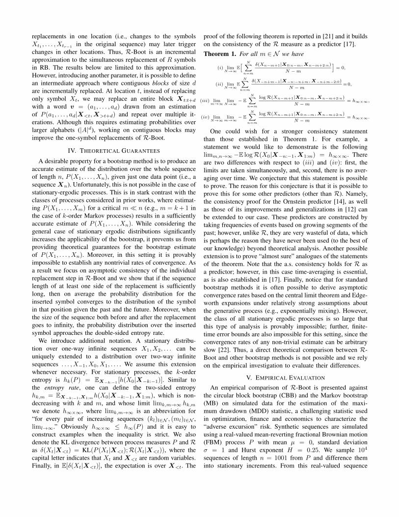
the order of MB is optimized in [1, 20]. Notice that such tuningis not possible in practice since only one sequence is availableand the true statistics of the process are obviously unknown.These best parameters for CBB and MB are intended to upperbound the performance that can be achieved by these methods.Furthermore, the best order for MB also represents an upperbound for any other method using a mixture of Markov modelswith different orders, such as a direct use of the R measurein Def. 3 to generate sequences sampling from P (Xt|X<t)or the sieve bootstrap [2] that automatically selects the order.Results. R-Boot, CBB and MB are compared on FBM datain Fig. 2. CBB is run with its best block width, while MBis run with its best model size. R-Boot is run with Kn =b1.5 log(n)c and two values for R, 0.75n and 3.5n. R-BootR = 0.75n achieves better performance than CBB and rawestimator θn = f(Xn) (single sequence), demonstrating thatapproximated replacement distributions are accurate enoughto guarantee bootstraps which resemble the original process.With this value of R RB still does not outperform MBwith the best (in hindsight) order. This is perhaps becauseR = 0.75n corresponds to approximately 30% replacementsto the original sequence which is not enough to generatesufficiently different sequences. In comparison, MB generatesbootstrapped sequences from scratch. With R = 3.5n thereplacements increase to approximately 140% and R-Bootsignificantly outperforms MB for all values of n. This demon-strates that, while sub-optimal value of the parameters result

1The optimal constant in O(n1/3) depends on the (unknown) autocovari-ance and spectral density functions of the process [15].

large difference of performance of both CBB and MB, R-Bootis quite robust, meaning with values of R in a wide range itconsistently outperforms CBB and MB by a significant margin.

100 200 300 400 500 600 700 800 900 1000

0.02

0.04

0.06

0.08

0.1

0.12

0.14

n

MSE

Single SequenceRBoot, R=0.75nRBoot, R=3.5nCBB(Optimal Block Width)MB(Optimal Model Size)

Fig. 2. MDD MSE (with standard errors) on FBM sequences.

REFERENCES[1] K. Bassler, J. McCauley, and G. Gunaratne. Nonstationary increments,

scaling distributions, and variable diffusion processes in financial mar-kets. Proc. National Academy of Sciences, 104(44):17287–17290, 2007.

[2] Peter Buhlmann et al. Sieve bootstrap for time series. Bernoulli,3(2):123–148, 1997.

[3] Bradley Efron. Bootstrap methods: Another look at the Jackknife. TheAnnals of Statistics, 1979.

[4] R. Gray. Probability, Random Processes, and Ergodic Properties.Springer Verlag, 1988.

[5] Peter Hall. The bootstrap and Edgeworth expansion. Springer, 1992.[6] Joel L Horowitz. The bootstrap. Handbook of econometrics, 5:3159–

3228, 2001.[7] Joel L Horowitz. Bootstrap methods for markov processes. Economet-

rica, 71(4):1049–1082, 2003.[8] J.-P. Kreiss and S. Lahiri. Bootstrap methods for time series. Handbook

of Statistics: Time Series Analysis: Methods and Applications, 30, 2012.[9] R. Krichevsky. A relation between the plausibility of information about

a source and encoding redundancy. Probl.Inf.Trans., 4(3):48–57, 1968.[10] RJ Kulperger and BLS Prakasa Rao. Bootstrapping a finite state markov

chain. Sankhya: The Indian Journal of Statistics, Series A, pages 178–191, 1989.

[11] Soumendra N Lahiri. Theoretical comparisons of block bootstrapmethods. Annals of Statistics, pages 386–404, 1999.

[12] G. Morvai, S. Yakowitz, and L. Gyorfi. Nonparametric inference forergodic, stationary time series. Ann. Stat., 24(1):370–379, 1996.

[13] Daniel J Nordman et al. A note on the stationary bootstrap’s variance.The Annals of Statistics, 37(1):359–370, 2009.

[14] Donald S Ornstein. Guessing the next output of a stationary process.Israel Journal of Mathematics, 30(3):292–296, 1978.

[15] Dimitris N Politis and Halbert White. Automatic block-length selectionfor the dependent bootstrap. Econometric Reviews, 23(1):53–70, 2004.

[16] B. Ryabko and V. Monarev. Experimental investigation of forecastingmethods based on data compression algorithms. Problems of InformationTransmission, 41(1):65–69, 2005.

[17] Boris Ryabko. Prediction of random sequences and universal coding.Problems of Information Transmission, 24:87–96, 1988.

[18] Boris Ryabko. Applications of Kolmogorov complexity and universalcodes to nonparametric estimation of characteristics of time series.Fundamenta Informaticae, 83(06):1–20, 2008.

[19] Boris Ryabko. Compression-based methods for nonparametric pre-diction and estimation of some characteristics of time series. IEEETransactions on Information Theory, 55:4309–4315, 2009.

[20] Boris Ryabko. Applications of universal source coding to statisticalanalysis of time series. Selected Topics in Information and CodingTheory, World Scientific Publishing, pages 289–338, 2010.

[21] A. Sani, A. Lazaric, and D. Ryabko. The replacement bootstrap fordependent data. Technical Report hal-01144547, INRIA, 2015.

[22] P. Shields. The Ergodic Theory of Discrete Sample Paths. AMS, 1996.[23] Kesar Singh. On the asymptotic accuracy of Efron’s bootstrap. The

Annals of Statistics, pages 1187–1195, 1981.

APPENDIX ACOMPUTATION OF THE REPLACEMENT DISTRIBUTION

In this section we report more details on how to actually compute the Replacement Bootstrap in Eq. 5 and we discuss itsoverall computational complexity.

Dealing with numerical issues. As illustrated in Eq. 5, the replacement probability that a (new) sequence has a symbola ∈ A in position t given that the rest of the sequence is as in the original Xn is calculated by estimating P (Xt = a|X<t,X>t)as

RXn(Xt = a|X<t,X>t) =

RXn(X<t; a;X>t)∑

c∈ARXn(X<t; c;X>t)=

∑∞i=0 ωiKiXn

(X<t; a;X>t)∑c∈A

∑∞j=0 ωjK

jXn

(X<t; c;X>t)

=

∞∑i=0

ωiKiXn(X<t; a;X>t)∑

c∈A∑∞j=0 wjK

jXn

(X<t; c;X>t)=

∞∑i=0

[∑c∈A

∞∑j=0

ωjωi

KjXn(X<t; c;X>t)

KiXn(X<t; a;X>t)

]−1. (6)

Although the previous expression could be computed directly by using the definition of the Krichevsky predictors, the valuesreturned by KjXn

(X<t; c;X>t) and KiXn(X<t; a;X>t) would rapidly fall below the precision threshold as n increases,

thus introducing significant numerical approximations. Therefore, we need to further elaborate the previous expression. Forany i, j 6= 0, let Y c = {X<t; c;X>t}, Y a = {X<t; a;X>t} be exactly as the original sequence with only the symbol atposition t replaced by symbol a and c ∈ A respectively, and let t′i,j = t+max{i, j}. In the following we exploit the fact that,conditionally on the frequency counts, the Krichevsky predictors of order m only uses the m symbols before to predict thecurrent symbol, so we obtain2

Kj(X<t; c;X>t)

Ki(X<t; a;X>t)=

n∏s=1

Kj(Y cs|Y c

<s)

Ki(Y as |Y a

<s)

=

t−1∏s=1

Kj(Y cs |Y c<s)

Ki(Y as |Y a<s)

n∏s=t

Kj(Y cs |Y c<s)

Ki(Y as |Y a<s)

=

t−1∏s=1

Kj(Xs|X<s)

Ki(Xs|X<s)

n∏s=t

Kj(Y cs |Y c<s)

Ki(Y as |Y a<s)

=

t−1∏s=1

Kj(Xs|Xs−j , . . . , Xs−1)

Ki(Xs|Xs−i, . . . , Xs−1)

n∏s=t

Kj(Y cs |Y cs−j , . . . , Y cs−1)Ki(Y as |Y as−i, . . . , Y as−1)

=

t−1∏s=1

Kj(Xs|Xs−j , . . . , Xs−1)

Ki(Xs|Xs−i, . . . , Xs−1)

t′i,j∏s=t

Kj(Y cs |Y cs−j , . . . , Y cs−1)Ki(Y as |Y as−i, . . . , Y as−1)

n∏s=t′i,j+1

Kj(Y cs |Y cs−j , . . . , Y cs−1)Ki(Y as |Y as−i, . . . , Y as−1)

=

t−1∏s=1

Kj(Xs|Xs−j , . . . , Xs−1)

Ki(Xs|Xs−i, . . . , Xs−1)

t′i,j∏s=t

Kj(Y cs |Y cs−j , . . . , Y cs−1)Ki(Y as |Y as−i, . . . , Y as−1)

n∏s=t′i,j+1

Kj(Xs|Xs−j , . . . , Xs−1)

Ki(Xs|Xs−i, . . . , Xs−1)

= πi,j,1:t−1

t′i,j∏s=t

Kj(Y cs |Y cs−j , . . . , Y cs−1)Ki(Y as |Y as−i, . . . , Y as−1)

πi,j,t′i,j+1:n,

where for any t1 and t2, we define

πi,j,t1:t2 =

t2∏s=t1

Kj(Xs|Xs−j , . . . , Xs−1)

Ki(Xs|Xs−i, . . . , Xs−1).

Notice that the previous expression is still valid for either i = 0 or j = 0 with the convention that K0(Y bs |Y b<s) = K0(Y bs ).

Thus, we obtain that Eq. 6 can be conveniently rewritten as

RXn(Xt=a|X<t,X>t)=

Kn∑i=0

[Kn∑j=0

ωjωiπi,j,1:t−1πi,j,t′i,j+1:n

(∑c∈A

t′i,j∏s=t

KjXn(Y cs |Y cs−j , . . . , Y cs−1)

KiXn(Y as |Y as−i, . . . , Y as−1)

)]−1. (7)

2In the following we drop the dependency on Xn.

We are now left with computing the expressions Ki(Ys|Ys−i, . . . , Ys−1) (for Y = Y a and Y = Y c) over the sequence ofvalues dependent on the replacement at t. As an illustrative case, let Ys = a and Ys−i, . . . , Ys−1 = V i, where V i is someword of length i, then

Ki(Ys|Ys−i, . . . , Ys−1) =νXn(a|V i) + 1/2∑

c∈A νXn(c|V i) + |A|/2=νXn(a|V i) + 1/2

νXn(Vi) + |A|/2

. (8)

Each term in the previous expression is computable with no major numerical error, since it stays in the range 2−i (and i shouldnever exceed Kn), and so the ratios between K values in Eq. 7 for each s and their products continue to be well conditioned.Even in the case that for some pairs i and j the numbers become too small, they are just added in the summation over c andj in Eq. 7, so this does not pose any numerical approximation problem anymore.Implementation details for Eq. 7 over successive replacements. In order to efficiently implement Eq. 7 over multiplereplacements, it is useful to store a series of intermediate values that will allow a small incremental computational cost fromone replacement to the other. Let K be a matrix of dimension (Kn+1)×n such that for any i = 0, . . . ,Kn and s = 1, . . . , n,

Ki,s = Ki(Xs|Xs−i, . . . , Xs−1).

We also define the multi-dimensional matrix R of dimensions (Kn + 1) × (Kn + 1) × n such that for any i, j = 0, . . . ,Kn

and s = 1, . . . , n,

Ri,j,s =Kj,s

Ki,s.

Then we compute πprev and πpost as

πi,j,prev =

t−1∏s=1

Ri,j,s, πi,j,post =

n∏s=t′i,j+1

Ri,j,s.

Similarly we define the multi-dimensional matrix K ′ of dimensions (Kn+1)× |A| × (tend− t) where tend = min{t′i,j , n} and

Ki,a,s = Ki(yas |yas−i, . . . , yas−1).Thus the matrix R′ of dimensions (Kn + 1)× (Kn + 1)× |A| × |A| × (tend − t) is

R′i,j,a,b,s =Kj,b,s

Ki,a,s.

Once these structures are computed, the final probability of replacement of a letter a in position t is computed as

R(Xt = a|X<t,X>t) =

Kn∑i=0

[ Kn∑j=0

wjwiπi,j,prevπi,j,post

(∑b∈A

t′i,j∏s=t

R′i,j,a,b,s

)]−1. (9)

As a result, the computational complexity for the first symbol replacement requires initializing the counts ν and coefficients πafter a full scan of the entire sequence Xn and the overall complexity is O(nK2

nA2). Nonetheless, it is possible to dramatically

reduce the computational complexity of the other steps.We use l = 1, . . . , L as an index for the replacement points, t(l) as the time index of the l-th replacement point, Zn(l)

as the sequence obtained after l replacement points (i.e., Zn(0) = Xn), and πi,j,prev(l) and πi,j,post(l) as the products ofprobabilities computed on the l-th sequence. Furthermore, we assume that the position of the replacement points is known inadvance (i.e., t(l) is chosen for all l = 1, . . . , L at the beginning). Beside πi,j,prev(0) and πi,j,post(0) at the first iteration l = 0,we also compute the additional structures

πi,j,prod(0) = πi,j,prev(0)× πi,j,post(0), πi,j,next(0) =

t′i,j(1)∏s=t(1)

Ri,j,s(0).

After the first replacement, only the coefficients πi,j,t1:t2 directly affected by the replacement of Xt by bt need to be recomputed.In particular, we notice that for any i = 1, . . . ,Kn and for any s such that s < t(l) or s > t(l)+ i then Ki,s(l+1) = Ki,s(l).Thus for any i we only need to recompute Ki,s for t(l) ≤ s ≤ t(l) + i. As a result, once the replacement is done and Z1

n iscomputed, the Ri,j,s affected by the change are recomputed and at the beginning of the new iteration we use them to compute

πi,j,cur(1) =

t′i,j(0)∏s=t(0)

Ri,j,s(1),

For any fixed i, j

πi,j,prev(l) πi,j,post(l)

t(l) t′i,j(l)

πi,j,prod(l) = πi,j,prev(l)× πi,j,post(l)

πi,j,prod(l + 1) =πi,j,prod(l)×πi,j,cur(l+1)

πi,j,next(l)

πi,j,next(l)

πi,j,curr(l + 1)

zl+1n

zln

t(l+1) t′i,j(l +1)

For any fixed i, j

πi,j,prev(l) πi,j,post(l)

t(l) t′i,j(l)

πi,j,prod(l) = πi,j,prev(l)× πi,j,post(l)

πi,j,prod(l + 1) =πi,j,prod(l)×πi,j,cur(l+1)

πi,j,next(l)

πi,j,next(l)

πi,j,curr(l + 1)

zl+1n

zln

t(l+1) t′i,j(l +1)

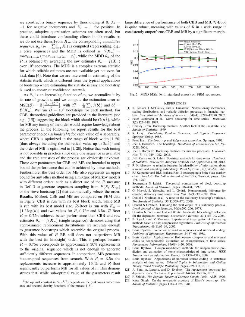
Fig. 3. Computation of other replacement points (i.e., l ≥ 1).

and this allows to compute the πprod terms of the next iteration as

πi,j,prod(1) =πi,j,prod(0)πi,j,cur(1)

πi,j,next(0),

In general, after the first iteration, at any iteration l ≥ 1, the computation of the previous elements can be done iteratively as(see also Fig. 3 for an illustration of these quantities)

πi,j,prod(l) =πi,j,prod(l − 1)πi,j,cur(l)

πi,j,next(l − 1),

where

πi,j,next(l) =

t′i,j(l+1)∏s=t(l+1)

Ri,j,s(l), πi,j,cur(l) =

t′i,j(l−1)∏s=t(l−1)

Ri,j,s(l).

As a result, while the complexity of recomputing the coefficients Ki,s for t(l) ≤ s ≤ t(l)+i, is limited to O(K2n) computations,

the overall computation for the replacement at each l > 0 is of order O(K3nA

2).

APPENDIX BPROOF OF THEOREM 1.

Proof. For the first statement, first note that,

E [δ(Xn−m+1|X0:n−m,Xn−m+2:n)] ≤ E [δ(Xn−m+1:n|X0:n−m)− δ(Xn−m+2:n|X0:n−m)] ≤ E [δ(Xn−m+1:n|X0:n−m)]

where the inequality follows from the fact that the KL divergence is non-negative. The statement follows from the consistencyof R as a predictor: for every m ∈ N we have (see [17, 18]).

limN→∞

1

NE

N∑n=m

δ(Xn−m+1:n|X0:n−m)→ 0. (10)

The proof of the second statement is analogous to that of the first, except that we need the consistency of R as a predictor“backwards,” that is, when the sequence extends to the past rather than to the future. The proof of this consistency is analogousto the proof of the usual (forward) consistency (10). Since it is important for exposing some further ideas, we give it here. Weconsider the case m = 1. The general case follows by replacing Yi = Xi:i+m for every i and noting that if the distribution ofXi is stationary ergodic then so is the distribution of Yi. We have

EN∑n=0

δ(X−n|X0:−n+1) = −N∑n=0

EX0:−n+1EX−n log

(R(X−n|X0:−n+1)

P (X−n|X0:−n+1)

)= −EX0:−N

log

(R(X−N :0)

P (X−N :0)

)= −E logR(X−N :0) + ElogP (X−N :0).

Since lim− 1NE logP (X−N :0) = h∞(P ), to establish the consistency statement it is enough to show that

lim− 1NE logR(X−N :0) = h∞(P ). For every k ∈ N

−E logR(X−N :0)−Nh∞(P ) = −E log

∞∑i=1

wi+1Ki(X−N :0)−Nhk(P ) +Nhk(P )−Nh∞(P )

≤ −E logKk(X−N :0)−Nhk(P )− logwk+1 +Nεk = o(N) +Nεk

where εk = hk(P ) − h∞(P ) and the last equality follows from the consistency of Kk. Since the statement holds for eachk ∈ N , it remains to notice that εk → 0.

The third statement follows from the first by noting that

Eδ(Xn−m+1|X0:n−m,Xn−m+2:n) = −E logR(Xn−m+1|X0:n−m,Xn−m+2:n) + hn,m,

and that by definition limn,m→∞ hn,m = h∞×∞. Analogously, the fourth statement follows from the second, where weadditionally need the stationarity of P to shift the time-index by n to the right.

APPENDIX CADDITIONAL EMPIRICAL RESULTS

A. Fractional Brownian Motion

Here we report additional experiments on the FBM model, a synthetic process commonly used to model complicated timeseries.

5 10 15 200

0.05

0.1

0.15

0.2

0.25

MS

E

Block Width

Single Sequence

Circular Block Bootstrap

2 4 6 8 10 12 140

0.05

0.1

0.15

0.2

0.25

MS

E

Markov Model Size (Order)

Single Sequence

MarkovBootstrap

100 200 300 400 500 600 7000

0.05

0.1

0.15

0.2

0.25

MS

E

R Percentage

Single Sequence

R-Boot

Fig. 4. Sensitivity analysis of CBB, MB, and R-Boot with respect to their parameters (block width, order, and number of replacements R)in the FBM experiment for n = 200 (notice the difference in scale for CBB).

Sensitivity analysis. In the results reported in the main text, we considered two values of the parameter R to show thatR-Boot is competitive w.r.t. the optimally tuned CBB and MB. In this section we explore the parameter sensitivity of thesethree methods, showing that advantage of R-Boot is potentially very important. In Fig. 4 we report the MSE performance ofeach method for a full range of parameters. CBB shows a very poor performance for block sizes that are too small while anincreasing block width improves performance. However, as noted in Section V above, CBB fails to demonstrate decisivelyimproved performance even against the single sequence estimator. On the other hand, MB significantly outperforms CBB andthe single sequence estimator. Fig. 4 illustrates the dependence of the performance of MB on the model size specified (theparameter corresponding to the order of the Markov source). Small orders introduce too much bias (i.e., the process cannotbe described accurately enough with 1 or 2-Markov models), while large orders suffer from large variance, where model sizesabove the optimal order overfit noise. As expected for a non-Markovian source, the best model size increases with n. Thuswe can conclude that properly tuning the order parameter for MB is challenging and a poor parameter significantly impactsperformance.

Finally, we report the performance of R-Boot w.r.t. the number of replacements. As discussed in Sect. III, R corresponds tothe number of attempted replacements. The need for large values is due to R-Boot’s sequential nature. In fact, as the sequenceZrn changes, the replacements in a specific position t may have different outcomes because of the conditioning in computingRXn

(·|Zr−1<tr ,Z

r−1>tr ). As a result, we need R to be large enough to allow for a sufficient number of actual changes in the

original sequence to generate a consistent bootstrap sequence. In order to provide an intuition about the actual replacements,let R′ be the number of times the value zr−1tr is changed across R iterations. For R = 0.75n, we obtain on average R′ ≈ 0.30n,meaning that less than 30% of the original sequence is actually changed. Similar results are observed from different valuesof R in both FBM and the real datasets. As illustrated in Fig. 4, both choices of R used in the experiments are suboptimal,

since the performance further improves for larger R (before deteriorating as the choice of R grows too large). Nonetheless,the change in performance is quite smooth and R-Boot outperforms both optimal block width CBB and optimal model sizeMB for a large range of R values.

B. Currency Data

In this section we report the result of testing R-Boot on differenced high-frequency 1-minute currency pair data. Currencypairs are relative value comparisons between two currencies. When differenced, these data can be considered close to beingstationary and ergodic [1]. From the application point of view, these data are suitable for testing analysis methods due to theirwide availability and since the underlying financial process is characterized by high liquidity, 24-hour nature and minimal gapsin the data due to non-trading times. This final feature is important because it reduces the noise caused by activities duringnon-trading hours, such as stock or economic news.

Estimator USDCHF EURUSD GBPUSD USDJPY

Asymptotic Estimator (single sequence) 93.0018 66.6727 72.8849 119.1314

Circular Block (optimal block width) 93.2946± 4.1490 66.9138± 3.5688 73.1951± 3.3746 119.2367± 6.6380

R-Boot (100% actual replacements) 44.6137± 5.1640 31.7459± 3.3220 37.0970± 4.5164 50.5639± 5.1623

Markov Bootstrap (optimal model size) 43.7268± 4.6376 29.4964± 3.0739 36.5849± 4.2520 47.5460± 4.7423

Fig. 5. MDD MSE (with 2X standard errors) on multiple high-frequency currency data.

We estimate the maximum drawdown statistic using bootstrap methods on four pairs of currencies considering the ratio ofthe first currency over the second currency. For example, the British Pound to U.S. Dollar cross is calculated as GBP/USD.We work with the 1-minute closing price. One minute data constitute a compressed representation of the actual sequence,which includes four data points for each 1 minute time interval: the open, high, low and close prices. The data3 used in thispaper were segmented into 1-day blocks of n = 1440 minutes. Days which were partially open due to holidays or announcedclosures were removed from the data set for consistency. A total of 300 days (1.5 years excluding holidays and weekends) ofdaily sequential samples from the underlying daily generative process were used for each currency pair.

10 20 30 40 50

40

50

60

70

80

90

100

MS

E

Block Width

Single Sequence

Circular Block Bootstrap

5 10 15 20

40

50

60

70

80

90

100

MS

E

Markov Model Size (Order)

Single Sequence

MarkovBootstrap

50 100 150 200 250 300 350

40

50

60

70

80

90

100

MS

E

R Percentage

Single Sequence

R-Boot

Fig. 6. Sensitivity to parameters for different bootstrap methods for the USDCHF currency (notice the difference in scale for CBB).

In Figure 5, we report estimation performance across all the currency datasets for MB with the best-performing order (withmodel size selected in [1, 20]), best block width CBB (with width selected in [1, 20]), and R-Boot with R = 3.5n (chosen tomatch the value used in the FBM experiments). As we noted in the FBM analysis, a large value of R does not necessarilycorrespond to a large value of replacements. In fact, we observed that the actual number of replacements in the FBM sequenceswith R = 3.5n were approximately 140% replacements. On these datasets, CBB exhibits constant behavior and can not beatthe simple baseline estimator (single sequence). On the other hand, R-Boot and MB significantly improve the maximumdrawdown estimation and they always perform similarly across different currencies (notice that the small advantage of MB is

3We downloaded the 1-minute historical data from http://www.forexhistorydatabase.com/

never statistically significant). The full range of parameters for each of these methods is reported in Fig. 6. These results mostlyconfirm the analysis in Section C-A, where MB achieves very good performance for a specific range of model sizes, whileperformance rapidly degrades in model sizes that are too large and too small. Finally, R-Boot confirms a similar behavior, asin the FBM, with a performance which gracefully improves as R increases with a gradual degradation thereafter.