the relative valuation - 50megsrdcohen.50megs.com/rvepi.pdf · 9 the relative valuation of an...

9The Relative Valuationof an Equity Price Index1

Ruben D. Cohen

A new approach for the relative valuation of an equity price index is presented. Themethod is based on a coordinate transformation or mapping, which enables one toweigh the index against the aggregated earnings and GDP. This, therefore, gives riseto the notion of relative valuation between the index, the earnings and the GDP. Apractical demonstration of this is then provided for the US, UK and Japan economiesand some of their major equity indices, namely the S&P500, FTSE100 and TOPIX,respectively.

Another potential application of the above is also discussed, which relates toforecasting the GDP. This stems from the assumption that the expected GDP, oneyear ahead from today, is readily priced in today’s interest rates. The method is furtherapplied to computing duration. This is shown to circumvent the difficulties that aregenerally associated with calculating the parameter.

1 IntroductionRelative valuation is a generic term that refers to the notion of comparing the price of an assetto the market value of similar assets. In the field of securities investment, the idea has ledto important practical tools, which could presumably spot pricing anomalies. Over time, thesetools have become instrumental in enabling analysts and investors to make vital decisions onasset allocation.

In equities, the concept separates into two areas—one pertaining to individual equities and theother to indices. The most common methodology for the former is based on comparing certainfinancial ratios or multiples, such as the price to book value, price to earnings, EBITDA toenterprise value, etc., of the equity in question to those of its peers (see, for instance, Barth et al.1998, D’Mello et al. 1991 and Peters 1991). This type of approach, which is largely popular asa strategic tool in the financial industry, is mainly statistical and based on historical data.

For an equity index, however, the above fails mainly because it is difficult to group indicesinto peer groups. Consequently, relative valuation here is generally carried out by comparing theindex’s performance to economic and market fundamentals, which may include GDP growth,

100 THE BEST OF WILMOTT 2

interest rate and inflation forecasts, as well as earnings growth, among others. This style ofcomparison is popular among practising economists in their attempt to rationalise the connectionsbetween the equity markets and the economy.

The above approach also has its faults, however—one being that, even if the fundamentalswere known, there appears to be no consensus methodology, as the procedures that are generallyimplemented tend to be subjective, ad hoc and dependent on personal style. Thus, it would beuseful to devise a new approach to enable one to add some objectivity to the process.

In constructing such a framework here, the classical equity valuation models are first sum-marised, after which the role of the equity risk premium and how it fits in are clarified. A coupleor so simple propositions are then brought in to help facilitate the process. The use of this newmethod is later demonstrated by (1) suggesting other potential applications, such as forecastingthe GDP and calculating duration and (2) incorporating it as a relative-valuation tool. It shouldbe noted that, owing to the nature of the approach, there is no need for any detailed statisticaltesting, as conclusions can be drawn simply by visual examination of graphs and charts alone.

2 A background on equity valuationSince the classical models of equity valuation are covered well in the literature, it would berepetitive to discuss them here in any depth. Nevertheless, it is still necessary to go over some ofthe assumptions and limitations that underlie these models, as they comprise part of the foundationupon which the new model for relative valuation is based.

2.1 The classical models of equity valuation

In the classical theory of equity valuation, three relationships dominate. They are:

Sf (t) − S(t)

S(t)+ δf (t)

S(t)= RM(t) (2.1)

δf (t) − δ(t)

δ(t)+ δf (t)

S(t)= RI (t) (2.2)

and

Ef (t)

S(t)= RF (t) (2.3)

where S(t) and δ(t), respectively, are the price and dividends at time t , while Sf (t), δf (t) andEf (t) signify the ‘expected’ price, dividends and earnings (after interest and tax, but beforedividends). These are yearly expectations, generated for one year ahead from today.

With regards to the above, note that, while Equation 2.1 is an identity, with RM(t) denoting theexpected total rate of return, Equations 2.2 and 2.3 represent valuation models, namely, Gordon’sGrowth Model2 and the discounted-cash-flow (DCF) relationship,3,4 respectively, with RI (t) andRF (t) being their expected discount rates. The equity risk premium is discussed briefly in thenext section, after which the derivation of the relative valuation model will be carried out.

RELATIVE VALUATION OF AN EQUITY PRICE INDEX 101

2.2 The equity risk premiumOwing to its importance in the area of equity investment, the equity risk premium has alwaysattracted attention from academics and practitioners. Countless papers have been written so far onthe subject, each proposing a reason for why the risk premium should exist, what it depends onand/or how large it should be. Although many of these works present conflicting theories and/orconclusions, all concur unanimously that the risk premium is a result of uncertainties. It is not theconcern here to discuss what causes these uncertainties. These uncertainties simply exist, havealways been and will remain to be around as long as no one can predict accurately what thefuture—near-term or far—holds for the economy and markets.

What is relevant here is how does the equity risk premium, as a parameter, get integrated intovaluation? By definition, the risk premium is the difference between the rate of return or discountrate, which could be any of the ones appearing in Equations 2.1–2.3 above, and some ‘risk-free’rate.5 As to what discount rate and risk-free rate one should use is another matter, which, again,shall be left out here. Rather, what is important is that under total and unconditional absence ofall uncertainty—past, present and future—the risk premium would not exist, so that all the ratesof return that appear in Equations 2.1–2.3 become equal to the ‘true’ risk-free rate, which itselfwould remain constant and free of volatility.6 This, therefore, leads to Proposition 1, which maybe expressed as:

Proposition 1 In the absence of all uncertainty and change—past, present and going for-ward—all risk premiums become zero.

Thus, what entails the above proposition is that all arbitrage opportunities between differenttypes of securities disappear. For instance, equity and fixed income instruments will yield thesame, as the yield curve flattens and becomes horizontal. In this instance, therefore, all yieldswill equal b∗, where b∗ symbolises the ‘true’ risk-free rate. Moreover, in the absence of the riskpremium, all rates of return (or discount rates) in Equations 2.1–2.3 will also equal b∗.

In addition to the above, the golden rule of economics enters also, so that

d ln G

dt=

(∂ ln G

∂t

)b=b∗=constant

= b∗ (2.4)

where G is the level of the nominal GDP and b is the interest rate, which is set constant at b∗.Finally, all forecasts in 2.1–2.3 above—i.e. Sf (t), δf (t) and Ef (t)—become identical to theirreal-time counterparts, S(t + 1), δ(t + 1) and E(t + 1), respectively, realised a year later at t + 1.

With Proposition 1 in place, Proposition 2 may now be stated as:

Proposition 2 Under Proposition 1, the golden rule applies also to the rate of growth inequity earnings.

Proposition 2 basically unites the golden rule, as it relates to the GDP in Equation 2.4, toequity earnings as well. This is possible under the above circumstances because equity earnings,or profits, comprise a subset of the GDP and, in the absence of arbitrage, all subdivisions withinthe GDP must yield at the same rate.

Quantitatively, this is expressible by(

∂ ln E

∂t

)b=b∗=constant

= b∗ (2.5)


where E is the equity earnings. Thus, under Propositions 1 and 2, with all rates of return in2.1–2.3 being equal to b∗, as well as the forecasts of S, δ and E remaining identical to theirreal-time counterparts a year later, Equation 2.5 may be applied to 2.3 to give:

(∂ ln E

∂t

)b=b∗

=(

∂ ln S

∂t

)b=b∗

= b∗ (2.6)

since, in this case, the discount rate, RF , also equals b∗.The implication of Equation 2.6, which states that, subject to the conditions imposed above,

the golden rule applies as well to the equity price, S(t), is significant. This is because, upon firstusing the approximation7

(∂ ln S

∂t

)b=b∗

≈ S(t + 1) − S(t)

S(t)(2.7)

then substituting 2.6 and 2.7 into 2.1 and, finally, setting the rate of return, RM(t), equal to b∗,all in the absence of the risk premium, the dividend yield, δ(t + 1)/S(t), tends to zero. Thissimply suggests that, in a world with no uncertainty and change, and, hence, no risk premiums,the investor will not demand any dividend yield.8

Therefore, do markets pay and/or investors demand a positive dividend yield because ofuncertainties? This, inevitably, points to the much debated issue of the dividend puzzle, alongwith its link to the equity risk premium, both of which will be left out here as they are notrelevant to this work, but, nonetheless, whose details may be found elsewhere (Cohen 2002).Notwithstanding, the above conclusions do lead to the next step, which is to develop a model forthe relative valuation of an equity price index.

3 A model for the relative valuation of an equityprice indexThe new model for relative valuation is constructed here in two ways—one focusing on equity(Section 3.1) and the other on the fundamentals, namely GDP and equity earnings (Section 3.2).The latter two occupy the same section because their underlying principles happen to be the same.The final results will then be united to present the relative valuation measures.

3.1 The equity modelBeginning here with Equation 2.6, which states

(∂ ln S

∂t

)b=b∗

= b∗ (2.6)

it follows that ln S could be written as a function of time, t , as well as b∗ —i.e.:

ln S = ln S(b∗, t) (3.1)

In the above, holding the discount rate constant at b∗ clearly imposes a severe constraint onS. This, however, may be relaxed by proceeding as follows. Very briefly, in place of writing


ln S(b∗, t) as done in 3.1, it shall be expressed as

ln S = ln S(b, t) (3.2)

which generalises S to account for a time-variable discount rate, b = b(t), instead.The rationale behind Equation 3.2 is that the effects of the market, and the economy in general,

on S are presumed to enter separately through two fundamental elements, one which is b and theother which comprises everything else that falls outside the reign of b. As the second variableappears as time, t , it renders Equation 3.2 general and, hence, together with b(t), it should captureall the economic and market effects on the price, S. In other words, expressing S in the form of3.2 effectively removes all the restrictions imposed on it earlier in Equation 3.1.

In view of the above, the total time differential of Equation 3.2, subsequently, becomes:

� ln S(b, t)

�t=

(∂ ln S

∂t

)b

+(

∂ ln S

∂b

)t

�b

�t(3.3)

where � denotes time-wise differential—i.e. �b ≡ b(t + 1) − b(t). While the first partial dif-ferential—i.e. (∂ ln S/∂t)b —has been shown to be equal to b (see Equation 2.6), the second,(∂ ln S/∂b)t , is simply the stock duration, which is the sensitivity of the price to changes in b atsome given point in time.

Being an ‘exact differential’, therefore, the two components in Equation 3.3 are coupled toeach other via:

(∂

∂b

(∂ ln S

∂t

)b

)t

=(

∂

∂t

(∂ ln S

∂b

)t

)b

(3.4)

Since, by virtue of 2.6, the left-hand side of the above is 1, the above equation simplifies to:

(∂

∂t

(∂ ln S

∂b

)t

)b

= 1 (3.5)

which may be integrated twice to yield a general solution of the form:

ln S = bt + α0 + α1b + �̃(b)

where α0 and α1 are integration constants and �̃(b) a yet unknown function of only b.Alternatively, the above may be recast into:

ln S − bt = �(b) (3.6)

where �(b) is another function of b. The latter representation conveniently absorbs �̃(b), α0 andα1b into a single function, �(b).

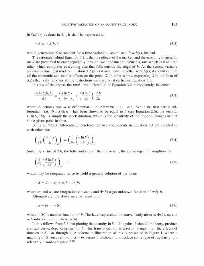
It thus follows from 3.6 that plotting the quantity ln S − bt against b should, in theory, producea single curve, depending only on b. This transformation, as a result, brings in all the effects oftime on ln S − bt through b. A schematic illustration of this is presented in Figure 1, where amapping of S versus b into ln S − bt versus b is shown to introduce some type of regularity to arelatively disordered graph.9,10


Ψ(b)

S

b

ln(S

) − b

t

b

maps into

Figure 1: Schematic of the convergence of data pointsunder the proposed coordinate transformation

In light of the derivation so far, it is necessary to mention two points. First, even thoughEquation 3.6 is extracted from what appears to be too theoretical an approach, it is indeed easyto apply to real situations and, also, as it shall be demonstrated shortly, it does possess otherpractical uses too. Second, questions relating to what b is—i.e. what interest rate should oneuse here—have undoubtedly been raised by now. The answer to these, as it will turn out later,happens to be straightforward. Beforehand, however, the same logic is applied next to both thenominal GDP and earnings, as similar transformations are derived.

3.2 Applications to GDP and earnings

It is well accepted that movements in the equity price index are tied closely to corporateearnings and, even more generally, to the economy. Common sense further dictates that abull market comes typically with a strong economy and a bear market with a weak one. Anexplanation for this correlation is that the market comprises a subset of the economy—i.e.corporate earnings constitute a (small) fraction of the GDP. This, therefore, should enableone to derive a GDP relationship analogous to the one for equity, as well as for corporateearnings.

Before going into that, however, we need to introduce, with the help of the DCF,11 a coupleof analogies to the equity price index. For this, define VG and VE as the ‘values’ associated withthe nominal GDP and corporate earnings, respectively.12 Therefore, under Propositions 1 and 2,VG could be represented by

VG ≡ Gf

b∗ (3.7a)

and VE by

VE ≡ Ef

b∗ (3.7b)

where Gf and Ef , respectively, are the time-t expectations of the nominal GDP and corporateearnings one year ahead, at t + 1. Hence, with b∗ analogous to the discount rate in a ‘constant’world, the DCF valuation model is being imposed on the economy as well. It should further bestressed that the one-year-ahead nominal GDP, i.e. G(t + 1), will from now on be implemented


instead of the expected for no reason other than convenience, as it shall be assumed that the twoconverge in an information-efficient economy. For the expected corporate earnings, Ef , on theother hand, Datastream’s aggregate I/B/E/S forecasts will be presumed sufficient for the purposesof this work.

Now, with the above analogy in place, it is simple to demonstrate that upon relaxing theconstraint on b∗ (i.e. replace b∗ with b, as it was done in going from Equation 3.1 to 3.2), thesame rules that govern the price index should apply as well to VG and VE , yielding expressionssimilar to Equation 3.6, but with VG and VE substituted for S. This, consequently, leads to:

ln VG − bt = �(b) (3.8a)

and

ln VE − bt = �(b) (3.8b)

where, as before, �(b) and �(b) are functions of only b.It should be emphasised that, even though the same transformation that presides over the

equity model applies to here as well, the functions �(b) and �(b) may not necessarily be thesame as �(b). A comparison of these will be made later; however, certain issues that this raises,namely of the interest rate, ‘reversibility’ and ‘structural or regime shifts’, must be addressedbeforehand.

3.2.1 Reversibility and structural shifts The representations for the equity price index, GDPand earnings, which are provided in Equations 3.6 to 3.8, lead to the important notions of‘reversibility’ and ‘structural shifts’. Recognising that structural shifts tend to alter the behaviourof the economy and the markets, an important objective here, as in any economic and finan-cial analysis, would thereby consist of defining ways for detecting and, possibly, classifyingthem.

To carry this out, observe that ln S − bt, ln VG − bt and ln VE − bt must depend solely on b

via the functions �(b), �(b), and �(b), respectively. The effect of time, as mentioned earlier,enters indirectly through b. Whether or not this functional dependence of �, � and � on b is thesame in all situations is not of concern now, but, eventually, it shall be dealt with.

An important by-product of such dependence is the concept of ‘reversibility’, which may beexplained via Figure 1 as follows. In reference to this figure, it is noted that, while the unmappedprice, S, varies with both b and t and leads to a scattered plot of S versus b, the mapped counterpartchanges only with b. This implies that if, for example, the price is S1 at time t1, when b equals,let us say, 5%, then at a later time t2, when b reverts back to 5%, the transformed parameters,ln S1 − bt1 and ln S2 − bt2, calculated at both times, t1 and t2, respectively, must reach the samevalue again, regardless of the path taken from 1 to 2. This, of course, should apply to VG and VE

as well, simply by virtue of Equations 3.8a and 3.8b.Alternatively, a structural or regime shift implies the contrary. If, for instance, a transformed

plot produces notably disparate lines, then it is likely that a structural shift has occurred somewherein between. Schematically, a structural shift is exemplified in Figure 2, where mapping S versusb into ln S − bt versus b over a given time frame leads to distinctive characteristic patterns. In asimilar manner, outliers should, under this type of transformation, appear as shown in Figure 3.Empirical evidence of these phenomena, namely reversibility, regime shifts and outliers, will beprovided in Section 4.


S

b

ln(S

) −

bt

b

maps into

Ψ2(b)Ψ1(b)

Figure 2: Schematic of how a regime shift manifests itself underthe suggested coordinate transformation. A mapping of S versus b

into ln S − bt versus b leads to distinctive characteristic functions,depicted here by �1(b) and �2(b), each belonging to a separateregime

S

b

ln(S

) −

bt

b

Ψ(b)

maps into

Outliers

Figure 3: Schematic of how outliers become visibleunder the suggested coordinate transformation. Amapping of S versus b into ln S − bt versus b shouldclearly separate outliers from the function, �(b)

3.2.2 The interest rate As mentioned at the end of Section 3.1, the issue of the interest rateis an important one. Putting it more precisely, what should one use for b in Equations 3.6 and3.8a,b in order to test their validity?

Obviously, several choices exist. These include all the different yields associated with thedifferent, available bond maturities, thus adding to the subjectivity. But, nevertheless, an attemptis made later to settle this point.

Upon following the steps that led to the coordinate transformations in Equations 3.6 and 3.8a,b,it is noted that (bond) maturity or tenor does not enter into the picture. Furthermore, in the contextof the reversibility property discussed earlier, it should also not matter which interest rate is used.In other words, using b as the yield of any bond maturity, be it 2 years or 7 years or 30 years,etc., should be acceptable, but only if one moves along a characteristic line, i.e. �(b), �(b), and�(b), which belongs to a certain structural regime. The invariance towards maturity should notbe expected to hold across regime shifts and/or to outliers.


4 Evidence of reversibility, outliers andstructural shiftsIf the hypotheses put forward above were to be proven valid, then upon plotting ln X − bt againstb, where X could signify S, VG or VE , one should expect to obtain a single curve, or, moregenerally, a series of curves, each pertaining to some particular structural regime in the marketand/or the economy. Furthermore, it was argued that b could represent the yield associated withany tenor. Examples of each of these, with specific applications to the US, UK and Japan (JP)economies and markets, will be provided in the following sections. Prior to this, however, onemust carefully study Table 1, which illustrates how the functions �(b), �(b), and �(b) arecalculated.

4.1 Applications to US data

To evaluate the long-run applicability of the model to the US market, refer to Figures 4a,b, wherein Figure 4a the S&P price data from 1950 to 200013 are plotted both in raw form, as S versus b,and transformed, as ln S − bt versus b, where b has been chosen to be the 10-year US governmentbond yield.14 It is evident here that the raw data, as plotted in Figure 4a, exhibit no regular pattern,whereas the mapped form in Figure 4b definitely displays a convergence that is consistent withtheory. A similar conclusion can be derived also from Figures 5a,b, where the aggregated earningsare displayed, both raw and transformed, over the same time period.15

Shorter-term, but more detailed, data (quarterly as opposed to annual) for the US, covering fromabout 1980 to 2004, are presented in Figures 6a–c, where evidence of all the above-mentionedeffects, namely convergence, regime shifts and outliers, are clearly depicted. In all instances thatfollow from now on, the data come from Datastream, using the codes tabulated in Table 2. Also,unless otherwise specified, b will be given by the 10-year government bond yield.

Figures 6a–c present plots of quarterly numbers pertaining to the S&P500 price, I/B/E/S earn-ings forecast and US GDP, respectively, comparing the raw data against their mapped counterparts.Convergence is noticeable in all cases, although the support is more compelling in the earningsand GDP plots shown in Figures 6b and 6c.

Figure 6a, which pertains to the price index, demonstrates how an outlier, which could other-wise remain hidden in the raw data, stands out in the mapped plane. The outlier highlighted hererepresents the quarter just before the August 1987 crash, when the overpricing in the S&P500index, which was then also present in many other national and international indices, led subse-quently to the crash.

Figures 6b and 6c, on the other hand, depict structural breaks and regime shifts in the aggre-gated earnings and GDP. In the interest of objectivity, however, as well as owing to the primaryfocus of this work, which is to introduce the capabilities of the model rather than guess the causesthat could have led to these shifts, there will be no further speculation here. An economist is, per-haps, better suited to undertake this task, by observing the timing of these breaks and connectingthem to fundamental (economic and/or market) changes that might have occurred then.

4.2 Applications to UK and JP data

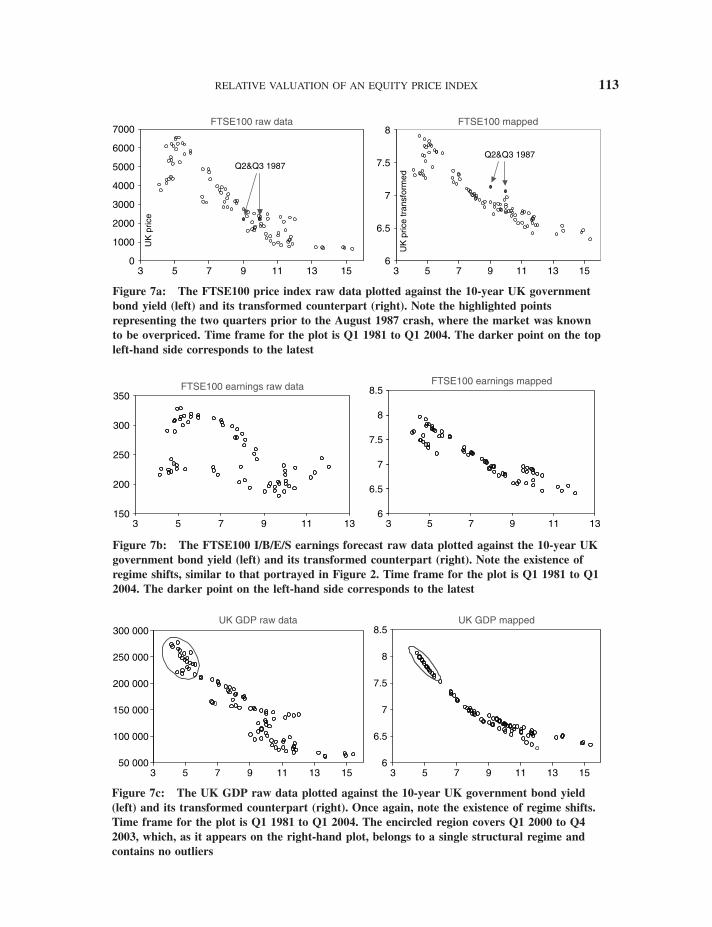
The UK data, concentrating on the FTSE100 price index, aggregated I/B/E/S earnings forecastsand GDP, are presented in Figures 7a–c, respectively. Once again, similar to the US case in


TA

BL

E1:

CA

LC

UL

AT

ION

OF

TH

EF

UN

CT

ION

S�

(b),

�(b

)A

ND

�(b

)F

RO

MD

OW

NL

OA

DE

DU

SD

AT

AO

FT

HE

S&P

500

PR

ICE

IND

EX

,S

,10

-YE

AR

YIE

LD

GO

VE

RN

ME

NT

BO

ND

YIE

LD

,b

,N

OM

INA

LG

DP

LE

VE

L,G

,A

ND

TH

EI/

B/E

/SA

GG

RE

GA

TE

EA

RN

ING

SF

OR

TH

EIN

DE

X,E

f.

DA

TE

OF

DO

WN

LO

AD

ISF

EB

RU

AR

Y12

,20

04.T

HE

SAM

PL

EC

AL

CU

LA

TIO

NS

INN

OT

ES

6–

10U

ND

ER

NE

AT

HT

HE

TA

BL

EA

RE

BA

SED

ON

Q1

2001

Dat

eS

(1)

b(2

)G

(3)

Ef

(4)

t(5

)V

G(b

)(6

)V

E(b

)(7

)�

(b)

(8)

�(b

)(9

)�

(b)

(10)

Q1

0013

46.0

96.

588

9629

.461

.134

1915

2167

.692

8.0

5.95

325.

2810

5.58

13Q

200

1437

.26.

556

9822

.863

.983

19.2

515

3877

.497

5.9

6.00

845.

2819

5.62

14Q

300

1491

.72

5.90

598

62.1

64.0

8819

.517

0977

.110

85.3

6.15

625.

4978

5.83

82Q

400

1367

.72

5.69

699

53.6

63.6

6819

.75

1789

65.9

1117

.86.

0959

5.57

005.

8941

>>

Q1

0113

01.5

35.

223

1002

4.8

60.7

3120

1977

65.7

1162

.86.

1267

5.75

026.

0140

Q2

0112

91.9

65.

398

1008

8.2

58.1

7320

.25

1931

88.2

1077

.76.

0708

5.67

835.

8895

Q3

0111

61.9

74.

924

1009

6.2

56.5

6920

.521

4094

.211

48.8

6.04

855.

8648

6.03

71Q

401

1138

.65

4.88

810

193.

952

.872

20.7

521

7342

.510

81.7

6.02

335.

8750

5.97

20Q

102

1104

.18

4.91

910

329.

354

.423

2121

8251

.711

06.4

5.97

395.

8604

5.97

59Q

202

1106

.59

5.23

910

428.

356

.385

21.2

520

7037

.610

76.3

5.89

585.

7274

5.86

80Q

302

928.

774.

2910

542

56.3

4221

.525

8904

.413

13.3

5.91

156.

1419

6.25

80Q

402

900.

364.

006

1062

3.7

55.3

0221

.75

2807

36.4

1380

.55.

9315

6.27

396.

3589

Q1

0385

1.17

3.93

1073

5.8

55.0

7822

#N/A

1401

.55.

8820

#N/A

6.38

07Q

203

944.

33.

447

1084

6.7

56.4

5722

.25

1637

.96.

0835

6.63

42Q

303

999.

744.

401

1110

758

.581

22.5

1331

.15.

9173

6.20

35Q

403

1034

.15

4.14

611

246.

360

.08

22.7

514

49.1

5.99

816.

3355

Q1

0411

51.8

24.

031

#N/A

62.2

2523

1543

.76.

1220

6.41

48

(1)

S&

P500

pric

ein

dex

(2)

US

10-y

ear

gove

rnm

ent

bond

yiel

d.(3

)N

omin

alle

vel

ofU

SG

DP

.(4

)I/

B/E

/Sea

rnin

gsfo

reca

st.

(5)

Ref

eren

cetim

e,w

ithQ

100

bein

gta

ken

as19

.T

hein

itial

valu

eha

sno

impa

ctw

hats

oeve

ron

the

fina

lre

sults

.Q

uart

erly

mov

emen

tsar

ein

step

sof

0.25

.(6

)C

alcu

latio

nof

VG

base

don

Equ

atio

n3.

7a,

i.e.

1977

65.7

=10

329.

3∗10

0/5.

223.

Not

eth

atth

eG

DP

fore

cast

attim

et,

Gf

(t),

ista

ken

asth

eva

lue

ofG

aye

arla

ter,

i.e.G

f(t

=20

)=

G(t

=21

) .(7

)C

alcu

latio

nof

VE

base

don

Equ

atio

n3.

7b,

i.e.

1162

.8=

60.7

31∗ 1

00/5.

223.

Not

eth

atth

eea

rnin

gsfo

reca

stat

time

t,E

f(t

),is

take

nas

the

I/B

/E/S

fore

cast

attim

et=

2.(8

)T

rans

form

edpr

ice,

base

don

Equ

atio

n3.

6.C

ompu

ted

as6.

1267

=ln

(130

1.53

)−

5.22

3∗20

/10

0.(9

)T

rans

form

edG

DP,

base

don

Equ

atio

n3.

8a.

Thi

sis

com

pute

dhe

reas

5.75

02=

ln(1

9776

5.7)

−5.

223∗

20/10

0−

5.4.

The

fact

orof

5.4

has

been

subt

ract

edat

the

end

toad

just

the

leve

lof

�(b

)to

abou

t�

(b).

(10)

Tra

nsfo

rmed

I/B

/E/S

earn

ings

fore

cast

,ba

sed

onE

quat

ion

3.8b

.C

ompu

ted

as6.

0140

=ln

(116

2.8)

−5.

223∗

20/10

0.


0

200

400

600

800

1000

1200

1400

0 5 10

(a)

15 20

Interest rate, %

S&

P p

rice,

$

(b)−16

−14

−12

−10

−8

−6

−4

−2

0

2

40 5 10 15 20

Interest rate, %

ln S

− r

t

Figure 4: Raw and transformed data, respectively, of the S&P price versus theinterest rate from 1950 to about 2000. Transformation of the price data is carriedout according to Equation 3.6

Figure 6a, the FTSE100 price index, when mapped, depicts outliers that coincide exactly withtime periods immediately prior to the August 1987 crash. In addition, evidence of structural breakscan also be observed in mapped plots of both earnings and GDP.

The JP data, which are included in Figures 8a–c, are substantially different. First, the impactof the transformation on the TOPIX price, as depicted in Figure 6a, is non-existent. Obviously,


0

10

20

30

40

50

0 5 10

(a)

15 20

Interest rate, %

Ear

ning

s, $

/yea

r

(b)−20

−15

−10

−5

0

50 5 10 15 20

Interest rate, %

ln(E

f/r)

− rt

Figure 5: Raw and transformed data, respectively, of the S&P aggregatedearnings versus the interest rate from 1950 to about 2000. Transformation ofthe earnings data is carried out according to Equations 3.7a and 3.8a

the TOPIX does not abide by the same rules that the S&P500 and FTSE100 indices do. As tothe reason for this, whether it is a different valuation technique that underlies the TOPIX or acomplete detachment between this index and the bond yield (i.e. inapplicability of Equation 3.2to the TOPIX) is not up for speculation here. What is clear altogether is that this approach doesnot work for the TOPIX and, hence, cannot be used here.


0

400

800

1200

1600

3 5 7 9 11 13

Q3 1987

S&P500 raw data

4.4

4.9

5.4

5.9

6.4

3 5 7 9 11 13

Q3 1987

S&P500 transformed

Figure 6a: The S&P500 price index raw data plotted against the 10-year US governmentbond yield (left) and its transformed counterpart (right). Note the highlighted pointrepresenting the quarter prior to the August 1987 crash, where the market was known to beoverpriced. Time frame for the plot is Q1 1981 to Q1 2004. The darker point on the topleft-hand side is the most current

10

20

30

40

50

60

70

3 5 7 9 11

S&P500 earnings raw data

4.5

5

5.5

6

6.5

7

3 5 7 9 11

S&P500 earnings mapped

Figure 6b: The S&P500 I/B/E/S earnings forecast raw data plotted against the 10-yearUS government bond yield (left) and its transformed counterpart (right). Note theexistence of a regime shift, similar to that portrayed in Figure 2. Time frame for the plotis Q1 1981 to Q1 2004. The darker point on the top left-hand side corresponds to the latest

2000

4000

6000

8000

10 000

12 000

3 5 7 9 11 13 15

US GDP raw data

4.4

4.9

5.4

5.9

6.4

3 5 7 9 11 13 15

US GDP mapped

Figure 6c: The US GDP raw data plotted against the 10-year US government bond yield(left) and its transformed counterpart (right). Once again, note the existence of regime shifts.Time frame for the plot is Q1 1981 to Q1 2004. The encircled region covers Q1 2000 to Q42003, which, as it appears on the right-hand plot, belongs to a single structural regime andappears to contain no outliers


TABLE 2: DATASTREAM CODES FOR THE QUARTERLYDATA USED IN FIGURES 6 AND THEREAFTER

Country Parameter Datastream code

S&P500 S&PCOMPI/B/E/S earnings forecast @:USSP500(A12FE)US GDP USGDP . . .B

US 30-year US gov. bond yld. BMUS30Y(RY)10-year US gov. bond yld. BMUS10Y(RY)7-year US gov. bond yld. BMUS07Y(RY)5-year US gov. bond yld. BMUS05Y(RY)2-year US gov. bond yld. BMUS02Y(RY)

FTSE100 FTSE100I/B/E/S earnings forecast @:UKFT100(A12FE)UK GDP UKGDP . . .B

UK 20-year UK gov. bond yld. BMUK20Y(RY)10-year UK gov. bond yld. BMUK10Y(RY)7-year UK gov. bond yld. BMUK07Y(RY)5-year UK gov. bond yld. BMUK05Y(RY)2-year UK gov. bond yld. BMUK02Y(RY)

TOPIX TOKYOSEI/B/E/S earnings forecast @:JPTOPIX(A12FE)JP GDP JPGDP . . .B

JP 30-year JP gov. bond yld. BMJP30Y(RY)10-year JP gov. bond yld. BMJP10Y(RY)7-year JP gov. bond yld. BMJP07Y(RY)5-year JP gov. bond yld. BMJP05Y(RY)2-year JP gov. bond yld. BMJP02Y(RY)

In contrast, however, a pattern does emerge when the I/B/E/S earnings forecasts are trans-formed, as shown in Figure 8b. Here, there is evidence of a structural shift in the earnings,coinciding to around the end of 1994 when the 10-year yield was approximately 4.5%. The JPGDP, on the other hand, which is illustrated in Figure 8c, displays a remarkably tight pattern,showing no signs of any structural change in the economy, at least from Q1 1984 to Q1 2004,the selected range of the data.

In the case of JP, therefore, one could conclude that bond yields (1) are completely detachedfrom the TOPIX price, (2) have an influence on expected earnings and (3) are tightly coupledto the GDP. This, subsequently, could mean that in Japan, the GDP and TOPIX price are notconnected to one another, so that any attempt to infer the direction of the TOPIX price, andpossibly other Japanese equity indices, from expected movements in either the interest ratesand/or the GDP is doomed to fail.

4.3 The impact of bond maturity

Having thus far concentrated only on the 10-year government bond yield, it is time now toquestion the applicability of the approach to other bond maturities. According to the governing


0

1000

2000

3000

4000

5000

6000

7000

3 5 7 9 11 13 15

UK

pric

e

Q2&Q3 1987

FTSE100 raw data

6

6.5

7

7.5

8

3 5 7 9 11 13 15

UK

pric

e tr

ansf

orm

ed

Q2&Q3 1987

FTSE100 mapped

Figure 7a: The FTSE100 price index raw data plotted against the 10-year UK governmentbond yield (left) and its transformed counterpart (right). Note the highlighted pointsrepresenting the two quarters prior to the August 1987 crash, where the market was knownto be overpriced. Time frame for the plot is Q1 1981 to Q1 2004. The darker point on the topleft-hand side corresponds to the latest

150

200

250

300

350

3 5 7 9 11 13

FTSE100 earnings raw data

6

6.5

7

7.5

8

8.5

3 5 7 9 11 13

FTSE100 earnings mapped

Figure 7b: The FTSE100 I/B/E/S earnings forecast raw data plotted against the 10-year UKgovernment bond yield (left) and its transformed counterpart (right). Note the existence ofregime shifts, similar to that portrayed in Figure 2. Time frame for the plot is Q1 1981 to Q12004. The darker point on the left-hand side corresponds to the latest

50 000

100 000

150 000

200 000

250 000

300 000

3 5 7 9 11 13 15

UK GDP raw data

6

6.5

7

7.5

8

8.5

3 5 7 9 11 13 15

UK GDP mapped

Figure 7c: The UK GDP raw data plotted against the 10-year UK government bond yield(left) and its transformed counterpart (right). Once again, note the existence of regime shifts.Time frame for the plot is Q1 1981 to Q1 2004. The encircled region covers Q1 2000 to Q42003, which, as it appears on the right-hand plot, belongs to a single structural regime andcontains no outliers


0

500

1000

1500

2000

2500

3000

JP 10y Gov't Bond Yld

TOPIX raw data

6.06.26.46.66.87.07.27.47.67.88.0

0 2 4 6 8


TOPIX mapped

0 2 4 6 8

Figure 8a: The TOPIX price index raw data plotted against the 10-year JP government bondyield (left) and its transformed counterpart (right). Note the absence of any convergence in themapped frame of reference. Time frame for the plot is Q1 1984 to Q1 2004. The darker point onthe left-hand side corresponds to the latest

0 2 4 6 8


TOPIX earnings raw data

4.5

5.5

6.5

7.5

8.5

9.5

0 2 4 6 8


TOPIX earnings mapped

0

10

20

30

40

50

60

70

Figure 8b: The TOPIX I/B/E/S earnings forecast raw data plotted against the 10-year JPgovernment bond yield (left) and its transformed counterpart (right). Note the existence of aregime shift, similar to that portrayed in Figure 2. Time frame for the plot is Q1 1984 to Q12004. The darker point on the top left-hand side corresponds to the latest

5.5

6

6.5

7

7.5

8

8.5

0 2 4 6 8

JP G

DP

Tra

nsfo

rmed

0 2 4 6 8

JP 10y Gov't Bond Yld JP 10y Gov't Bond Yld

JP GDP raw data JP GDP mapped

2.5E+05

3.5E+05

4.5E+05

5.5E+05

Figure 8c: The JP GDP raw data plotted against the 10-year JP government bond yield (left)and its transformed counterpart (right). Note the absence of regime shifts in the transformedplane, which covers the period Q1 1984 to Q4 2003


equations 3.6–3.8, bond maturity, T , plays no role in the model. Therefore, going back toSection 3.2.2, this means that, in the absence of outliers and structural shifts, the characteristicline of convergence in the mapped frame of reference should remain insensitive to the differentmaturities. More simply stated, all points that result from applying the coordinate transformationusing yields from different bond maturities should, under the above conditions, fall exactly on thesame line, regardless of maturity.

The validity of the above may now be examined, again visually, by producing plots similar toFigures 6–8. In doing so, care must be taken to select regions where structural shifts and outliersare absent, of which the area encircled in Figure 6c is one. This region contains the time frameQ1 2000 to Q4 2003 for the US GDP. Bearing in mind that the graph was constructed using the10-year US government bond yield, we now ask what happens if different maturities were alsoincluded in the same plot.

The impact of bond maturity on, or rather the absence of its effect in, the present model isclearly demonstrated in Figures 9a–c, which enlarge the areas highlighted in Figures 6c, 7c and8c, for the US, UK and JP,16 respectively. In each of these figures, 9a–c, different governmentbond tenors—namely the 2, 5, 7, 10 and 30 years (20 instead of 30 years in the case of UK)—wereplotted together, with the idea that any observable scatter could be attributed to the differencesin maturities. Nevertheless, one obtains in all cases a remarkably tight fit, which provides furthertestimony to the earlier presumption (see Section 3.2.2) that the underlying curve is invariant todifferent maturities.

5 Potential applicationsPrior to going forward with the development of the relative valuation model, two types of appli-cations are brought to mind, both of which could have possible uses in the field of investment.

5

5.5

6

6.5

7

7.5

8

1.5 2.5 3.5 4.5 5.5 6.5

US 30-y yldUS 10-y yldUS 7-y yldUS 5-y yldUS 2-y yld

Figure 9a: The transformed US GDP for the area circled in Figure 6c,covering the time frame Q1 2000 to Q4 2003. The plot shows differentmaturities superimposed on each other. The horizontal and verticalcoordinates represent b and ln VG − bt , respectively


7.2

7.6

8

8.4

3.7 4 4.3 4.6 4.9 5.2 5.5 5.8 6.1 6.4

UK 20-y yldUK 10-y yldUK 7-y yldUK 5-y yldUK 2-y yld

Figure 9b: The transformed UK GDP for the area circled inFigure 7c, covering the time frame Q1 1998 to Q4 2003. The plotshows different maturities superimposed on each other. Thehorizontal and vertical coordinates represent b and ln VG − bt ,respectively

5

6

7

8

9

10

11

12

13

0 1 2 3 4 5 6 7 8

JP 30-y yldJP 10-y yldJP 7-y yldJP 5-y yldJP 2-y yld

Figure 9c: The transformed JP GDP for all of the area in Figure 8c,covering the time frame Q1 1984 to Q4 2003. The plot shows differentmaturities superimposed on each other. The horizontal and verticalcoordinates represent b and ln VG − bt , respectively

These applications, which are described next, result from the properties of the curves describedin Section 4 and consist of forecasting the GDP and calculating the duration.

5.1 Forecasting the GDPTo illustrate the GDP forecasting capability of the model, one needs to combine Equations 3.7aand 3.8a, replace b∗ by b and arrange the result as:

Gf (t) = exp[�(b) + bt + ln b] (5.1)


Recognising that Gf (t) is the GDP expectation, Equation 5.1 then allows one to recover theexpected GDP, one year from today, given today’s yield, b, as well as the empirically deter-mined function, �(b), which is extractable from plots similar to Figures 9a–c. The assumptionsunderlying this method are that (1) today’s bond yields have the expected GDP priced in themand (2) between now and one year ahead from now, no structural shifts will occur, so that thefunction �(b) retains its shape over the time period between now and then.

Let us now apply Equation 5.1 to the three cases of interest here, namely the US, UK and JP.Focusing initially on the US, it is observed that a fourth-order polynomial curve runs satisfactorilythrough all the points in Figure 9a, comprising the yields associated with the different tenors. Thiscurve, therefore, provides an empirical relation for �(b) with an R2 of 0.99975. The tightness ofthe fit is noteworthy in Figure 10a, where the polynomial expression is also included.

What follows now is a step-by-step demonstration of how a forecast for the US GDP, let’ssay of Q1 2005,17 could be obtained using Equation 5.1. (1) Compute from Table 1 the mappingof GDP to �(b). This, when plotted against b, leads to Figure 10a. (2) A curve fit, similar tothe one in that figure, could then be obtained to represent the behaviour of �(b) with respect tob. In this case, a fourth-order polynomial was sufficient to achieve a very tight fit. (3) Return toEquation 5.1 and note that the expected GDP for Q1 2005—i.e. Gf (t = Q1 2004)—may nowbe calculated by substituting the values of b, �(b) and the quantity bt, where, in correspondenceto Q1 2004, b and t are 4.031% and 23, respectively (see Table 1).

Repeating the above procedure for the different bond maturities leads to Figure 10b, as wellas Table 3, where different estimates of the Q1 2005 expected GDP have been obtained. Thesefall between 11 350 and 11 906 (in appropriate units), which correspond to the stretch of tenorsbetween 2 and 30 years, respectively. A simple average finally provides an overall estimate of11 619 for the Q1 2005 US GDP. Note that, since this value is based on yields that are marketdriven and which tend to vary rather gently on a day-to-day basis, the estimate for one-year-aheadGDP should also behave similarly.

7.5

8

7

6.5

6

5.5

51.5 2.5 3.5 4.5 5.5 6.5

US 30-y yldUS 10-y yldUS 7-y yldUS 5-y yldUS 2-y yld

y = 8.3886E − 04x4 − 1.8464E − 02x3 + 1.7972E − 01x2 − 1.2308E + 00x + 9.2779E + 00R2 = 9.9975E − 01

Figure 10a: Same as Figure 9a, but with a fourth-orderpolynomial curve fit passing through the yields belonging to thedifferent maturities indicated in the legend. The extremely tight fit,as reflected by the high R2, represents the function �(b)


8000

9000

10 000

11 000

12 000

13 000

14 000

15 000

16 000

1 2 3 4 5 6

US

GD

P

Yield, %2-

year

5-ye

ar

7-ye

ar

10-y

ear

30-y

ear

Figure 10b: The expected US GDP for Q1 2005 as a function ofthe interest rate, as derived from the methodology outlined inSection 5.1. The vertical lines correspond to the different maturityyields as of the time of data download—i.e. February 12, 2004,corresponding to Q1 2004

TABLE 3: EXAMPLE CALCULATION ILLUSTRATING THE GDP FORECASTINGPROCEDURE. A VALUE OF 23, CONSISTENT WITH THAT IN TABLE 1, WAS USED HEREFOR t TO SIGNIFY Q1 2004. ALSO, �(b) WAS COMPUTED USING THE POLYNOMIAL FIT INFIGURE 10a

Maturity, T Bond yield, b, in % bt/100 �(b) Expected GDP for Q1 05

2 years 1.687 0.38801 7.63116 11 3505 years 2.998 0.68954 6.77352 11 5667 years 3.544 0.81512 6.48367 11 60110 years 4.031 0.92713 6.24891 11 67130 years 4.911 1.12953 5.86892 11 906

Average 11 619

To validate these estimates, a back test was performed following the same steps as above.Here, for instance, an estimate for the now historical Q1 2001 GDP level is obtainable fromthe yields of Q1 2000, as well as upon utilising the same expression for �(b). This back testprovides Figures 11a–c, which pertain to the US, UK and JP, respectively. The basis of this isTable 4, which displays the fitted polynomials, as well as the time frames involved, for all threejurisdictions.

5.2 Calculating the durationIn the financial literature, the duration of any parameter, let’s say X, is defined as its sensitivityto the interest rate, keeping all else constant. Thus, quantitatively, the duration of X, symbolisedhere by DX, is represented by

DX ≡(

∂ ln X

∂b

)t

(5.2)


Although simplistic in construct, problems abound when trying to calculate DX in practice. First,since this application involves differentiation, then differentiating any volatile economic or marketfundamental, such as the GDP, price, earnings, etc., will lead to even more volatile outcomes. Sec-ond, the above definition incorporates a partial differentiation with respect to b, which explicitlyrequires holding the time parameter, t , constant. This is an impossible feat to achieve in practicesince expressing Equation 5.2 as the difference, let’s say, in GDP level between Q1 2001 and Q1

9500

10 000

10 500

11 000

11 500

12 000

Q1

01

Q2

01

Q3

01

Q4

01

Q1

02

Q2

02

Q3

02

Q4

02

Q1

03

Q2

03

Q3

03

Q4

03

Q1

04

Q2

04

Q3

04

Q4

04

Q1

05

US GDP forecast

Figure 11a: The US GDP forecast post-Q3 2003 derived by themethodology outlined in Section 5.1. The historical data, which arethe solid circles, are also included to demonstrate the close fitbetween model and data

220 000

230 000

240 000

250 000

260 000

270 000

280 000

290 000

300 000

Q4

99

Q1

00

Q2

00

Q3

00

Q4

00

Q1

01

Q2

01

Q3

01

Q4

01

Q1

02

Q2

02

Q3

02

Q4

02

Q1

03

Q2

03

Q3

03

Q4

03

Q1

04

Q2

04

Q3

04

Q4

04

Q1

05

UK GDP forecast

Figure 11b: The UK GDP forecast post-Q3 2003 derived by the methodology outlined inSection 5.1. The historical data, which are the solid circles, are also included to demonstrate theclose fit between model and data


430 000

450 000

470 000

490 000

510 000

530 000

550 000

570 000

Q4

01

Q1

02

Q2

02

Q3

02

Q4

02

Q1

03

Q2

03

Q3

03

Q4

03

Q1

04

Q2

04

Q3

04

Q4

04

Q1

05

JP GDP forecast

Figure 11c: The JP GDP forecast post-Q3 2003 derived by the methodology outlined inSection 5.1. The historical data, which are the solid circles, are also included to demonstrate theclose fit between the model and data

TABLE 4: TIME FRAMES, MATURITIES, POLYNOMIAL FITS AND THE R2 VALUESUNDERLYING THE CURVES IN FIGURES 9a–c

Market Time frame Maturities 4th order polynomial curve fit R squaredof data used

US Q1 00 - Q1 04 2, 5, 7, 10, 30 8.3886E − 04∗b ∧ 4 − 1.8464E − 02∗b ∧ 3 +1.7972E − 01∗b ∧ 2 − 1.2308∗b + 9.2779

99.975%

UK Q4 98 - Q1 04 2, 5, 7, 10, 20 −3.730118E − 03∗b ∧ 3 + 8.758313E − 02∗b ∧2 − 0.9.961051∗b + 11.10780

99.932%

JP Q3 00 - Q1 04 5, 7, 10, 30 0.1246∗b ∧ 4 − 0.9396∗b ∧ 3 + 2.7093∗b ∧ 2 −4.2651∗b + 10.509

99.960%

2000 divided by the yield b, will, implicitly, also involve a change in the time parameter. Thus,there is no way in practice that the above expression could be worked out.

Therefore, how could one get around this? Assuming for the time being that X is the GDPlevel, then, obviously, with �(b) being independent of time, the duration of the GDP—i.e. itssensitivity with respect to the interest rate while holding all else constant—could be computedby simply applying the partial differentiation to it. This yields the expression

DGDP =(

∂ ln Gf (t)

∂b

)t

= �′(b) + t + 1

b(5.3)


which greatly simplifies the calculation of the duration of GDP, among other data of interest. Inpractice, therefore, if one were to calculate the sensitivity of the GDP in Q1 2005 with respectto b, then it could be achieved from the above using �(b) in Table 4, along with the appropriatevalue for t , which, for example, is 23 for the US, in accordance to Table 1. This approachis mathematically more sound than the existing ones simply because the time parameter, t , isliterally being held constant in the process of calculating duration.

6 The relative valuation of an equity price index

Thus far, the model has been developed and applied to forecasting the GDP and computingduration. What remains now is its implementation to relative valuation. This is simple as it onlyinvolves superimposing the three empirically determined functions, �(b), �(b) and �(b), directlyon top of one another and looking for regions of deviation. It should be noted that this methodincorporates no adjustable parameters, except for a basic and necessary one that is discussed innote 9 under Table 1.18 To illustrate how the model works, we start with a preliminary description,along with a couple of historical examples, and then proceed with some detailed assessments.

6.1 A long-term historical example

For a preliminary demonstration, refer to Figures 4a and 4b, where, respectively, the historicalprice and earnings are mapped against the US government 10-year bond yield. A direct super-position of the two plots leads to Figure 12a, part of which has been magnified in Figure 12b.

Without dwelling too much on this, it is worth noting that the two data series, when mappedas �(b) and �(b) and superimposed, do fall on top of one another over most of the time covered,thus confirming that, with the exception of the period between 1950 and 1960, price and earningsare reasonably valued relative to each other. This chart, nevertheless, is based on annual data and,hence, does not capture the details that are to follow shortly.19 Before going into these, however,it is worth alluding to an issue that comes up often in related literature—namely, Irving Fisher’sassertion that the stock market was not overvalued just before its crash in 1929. An examinationof this is carried out in the next section.

6.2 Irving Fisher and the 1929 stock market crash

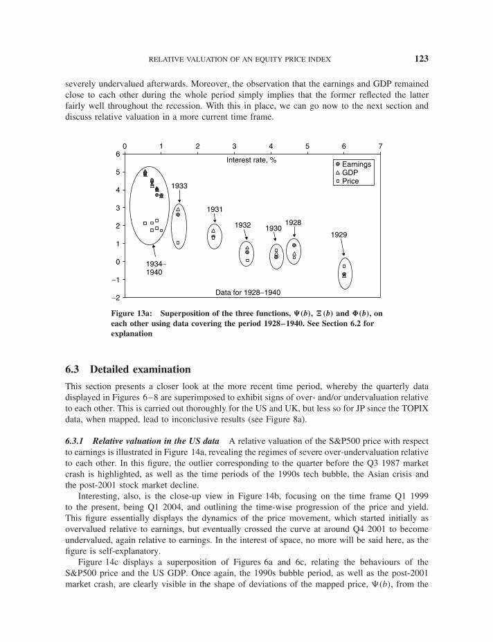
Let us now apply the model to provide an answer to a long-debated issue, which is whetherFisher was right in his claim that the stock market was not overvalued before its dramatic crashin 1929, around the time when the great depression began. This issue seems to be a popular one,as countless papers have been written on it, each attempting to offer an explanation (see, forexample, McGrattan and Prescott (2003) and references therein). We shall also try to provide ananswer here, albeit strictly in the context of the present model.

Refer to Figure 13, which portrays a superposition of the three functions, �(b), �(b) and�(b), on each other over the time period 1928–1940. Any deviation observed in this mapped planeshould, therefore, reflect the degree of relative valuation between the three fundamentals—beingprice, earnings and GDP.

First, note that from 1928 to 1931, all three fundamentals lie, more or less, near each other,signifying relative fair valuation. The significant deviation, which can be seen as a drop in the


−20

−15

−10

−5

0

5

100 5 10 15 20

PriceEarnings

Interest rate, %

19601950

Figure 12a: Figures 4b and 5b superimposed, portraying the notion of relativevaluation in the context of this work. Note that the points lie, more or less, ontop of one another except for the time frame between 1950 and 1960, duringwhich the convergence was in the process of happening

−7

−6

−5

−4

−3

−2

−1

0

1

2

3

4

51 3 5 7 9

PriceEarnings

Interest rate, %

19601950

1999

Figure 12b: Magnification of the boxed data in Figure 12a, illustrating theconvergence of the two characteristic functions, i.e. �(b) and �(b), ataround 1960

mapped price relative to the others, begins at around 1932 and becomes dramatic afterwards.Nevertheless, the mapped earnings and GDP remain reasonably close to one another throughoutthe whole time period. This, according to the model, means that, just before its plunge, theprice was not overvalued20 in relation to the earnings and GDP, but, nevertheless, it did become


severely undervalued afterwards. Moreover, the observation that the earnings and GDP remainedclose to each other during the whole period simply implies that the former reflected the latterfairly well throughout the recession. With this in place, we can go now to the next section anddiscuss relative valuation in a more current time frame.

−2

−1

0

1

2

3

4

5

60 1 2 3 4 5 6 7

EarningsGDPPrice

1929

1931

19301932

Data for 1928−1940

Interest rate, %

1933

1928

1934−1940

Figure 13a: Superposition of the three functions, �(b), �(b) and �(b), oneach other using data covering the period 1928–1940. See Section 6.2 forexplanation

6.3 Detailed examination

This section presents a closer look at the more recent time period, whereby the quarterly datadisplayed in Figures 6–8 are superimposed to exhibit signs of over- and/or undervaluation relativeto each other. This is carried out thoroughly for the US and UK, but less so for JP since the TOPIXdata, when mapped, lead to inconclusive results (see Figure 8a).

6.3.1 Relative valuation in the US data A relative valuation of the S&P500 price with respectto earnings is illustrated in Figure 14a, revealing the regimes of severe over-undervaluation relativeto each other. In this figure, the outlier corresponding to the quarter before the Q3 1987 marketcrash is highlighted, as well as the time periods of the 1990s tech bubble, the Asian crisis andthe post-2001 stock market decline.

Interesting, also, is the close-up view in Figure 14b, focusing on the time frame Q1 1999to the present, being Q1 2004, and outlining the time-wise progression of the price and yield.This figure essentially displays the dynamics of the price movement, which started initially asovervalued relative to earnings, but eventually crossed the curve at around Q4 2001 to becomeundervalued, again relative to earnings. In the interest of space, no more will be said here, as thefigure is self-explanatory.

Figure 14c displays a superposition of Figures 6a and 6c, relating the behaviours of theS&P500 price and the US GDP. Once again, the 1990s bubble period, as well as the post-2001market crash, are clearly visible in the shape of deviations of the mapped price, �(b), from the


mapped GDP, �(b). Finally, for the US, Figure 14d portrays the mapped S&P500 earnings, �(b),relative to the US GDP. Here, the period coinciding with the 1990s equity bubble is portrayedby a structural regime shift in the shape of a series of earnings data points that fall parallel to,but slightly above, the mapped GDP. Interestingly, however, the post-2001 decline in the marketprice, which is clearly apparent in Figure 14a, is not reflected at all by the earnings. This supports

4.5

4.7

4.9

5.1

5.3

5.5

5.7

5.9

6.1

6.3

6.5

3 4 5 6 7 8 9 10 11 12 13

S&P500 mapped priceS&P500 mapped earnings

US 10-year gov't bond yld

Tech bubble of the 1990s

Post-2001 crash

Q3 1987

Asian Crisis

Figure 14a: Relative valuation of the S&P500 price and earnings via superposition ofFigures 6a and 6b. Regions of gross deviation are circled. The 1990s tech bubbleportrays overvaluation of the stocks relative to earnings and the post-2001 crashshows undervaluation of the former relative to the latter

5.0335.735

5.9286.057

6.5886.556

5.9055.696

5.2235.3984.9244.888

4.919

5.2394.294.0063.93

3.447

4.401

4.146

4.031

5.6

5.9

6.2

6.5

6.8

3 3.5 4 4.5 5 5.5 6 6.5 7

Q1 99Q2 99Q3 99Q4 99Q1 00Q2 00Q3 00Q4 00Q1 01Q2 01Q3 01Q4 01Q1 02Q2 02Q3 02Q4 02Q1 03Q2 03Q3 03Q4 03Q1 04

1237.281333.321332.841424.941346.091437.2

1491.721367.721301.531291.961161.971138.651104.181106.59928.77900.36851.17944.3

999.741034.151151.82

5.0335.7355.9286.0576.5886.5565.9055.6965.2235.3984.9244.8884.9195.2394.29

4.0063.93

3.4474.4014.1464.031

S&P500 mapped earningsS&P500 mapped price


Figure 14b: Close-up of Figure 14a, covering the period Q1 1999 to Q1 2004 and depicting themovement of the mapped price relative to mapped earnings. The table on the right-hand sidelists the quarter, price and 10-year government bond yield in columns 1, 2 and 3, respectively


4.4

4.7

5

5.3

5.6

5.9

6.2

6.5

3 5 7 9 11 13 15

S&P500 mapped priceUS mapped GDP


Q3 1987

Figure 14c: Relative valuation of the S&P500 price and the US GDP via superposition ofFigures 6a and 6c

4.4

4.8

5.2

5.6

6

6.4

3 4 5 6 7 8 9 10 11 12 13

US mapped GDPS&P500 mapped earnings


Figure 14d: Relative valuation of the S&P500 earnings and the US GDP viasuperposition of Figures 6b and 6c

the claim, albeit in retrospect, that the rise in the market’s equity price during the 1990s wasnothing but a bubble, which ultimately collapsed.

6.3.2 Relative valuation in the UK data Figure 15a, which is a superposition of Figures 7aand 7b, displays the relative behaviour of the FTSE100 price against earnings, both in transformed


6

6.5

7

7.5

8

8.5

3 5 7 9 11 13 15

FTSE100 mapped priceFTSE100 mapped earnings

UK 10-year gov't bond yld

Post-2001 crash

Q3 1987

Figure 15a: Relative valuation of the FTSE100 price and earnings via superpositionof Figures 7a and 7b. Regions of gross deviation are circled. In contrast to theS&P500 case in Figure 14a, the 1990s tech bubble is completely absent and astructural shift in both price and earnings appears to have occurred post-2001

4.5044.835

5.2015.119

5.6025.472

5.2724.943

5.1114.8234.672

4.913

5.3354.671

4.5564.207

4.1294.538

4.9144.791

FTSE100 mapped priceFTSE100 mapped earnings

UK 10-year gov't bond yld7

7.2

7.4

7.6

7.8

8

8.2

4 4.3 4.6 4.9 5.2 5.5 5.8

5.082

Q1 99Q2 99Q3 99Q4 99Q1 00Q2 00Q3 00Q4 00Q1 01Q2 01Q3 01Q4 01Q1 02Q2 02Q3 02Q4 02Q1 03Q2 03Q3 03Q4 03Q1 04

6074.96206.436201.786550.756164.966232.956543.666440.1

6088.285914.985342.135290.985154.295217.984329.974115.993729.544049.014272.124354.74442.9

4.5044.8355.2015.1195.6025.4725.2725.0824.9435.1114.8234.6724.9135.3354.6714.5564.2074.1294.5384.9144.791

Figure 15b: Close-up of Figure 15a, covering the period Q1 1999 to Q1 2004 and depicting themovement of the mapped price relative to mapped earnings. The table on the right-hand sidelists the quarter, price and 10-year government bond yield in columns 1, 2 and 3, respectively

planes, throughout roughly the last 20 years. The data point pertaining to the quarter prior to theQ3 1987 crash is, once again, highlighted. Here, however, in contrast to the S&P case discussedin Section 6.1.1 and illustrated in Figure 14a, there is no sign, whatsoever, of a price bubble.

In the 1990s, during the peak of the dotcom bubble in the US, the FTSE100 price is observedto follow the earnings consistently. In this case, however, what coincides with the collapse of the


6

6.5

7

7.5

8

8.5

3 5 7 9 11 13 15

FTSE100 mapped priceUK mapped GDP


Q3 1987

Figure 15c: Relative valuation of the FTSE100 price and the UK GDP viasuperposition of Figures 7a and 7c

6

6.5

7

7.5

8

8.5

3 5 7 9 11 13 15


UK mapped GDP

FTSE100 mapped earnings

Figure 15d: Relative valuation of the FTSE100 earnings and the UK GDP viasuperposition of Figures 7b and 7c

price bubble in the S&P is a regime shift in the FTSE100 mapped earnings, which appears alsoto pull the FTSE100 price with it. This is further confirmed in Figure 15b, where the time-wisemovements in earnings and price are depicted in close-up. Again, as in the above and in theinterest of remaining objective, we shall not speculate here on the possible reasons for this regimeshift (in the behaviour of the earnings and the subsequent fall in the FTSE100 price). Rather, aneconomist is perhaps better suited to provide an explanation for this.


The lack of a tech bubble, similar to that in the S&P data, in the FTSE price index is againverified in Figure 15c, where the mapped price in Figure 7a is superimposed on the mappedUK GDP in Figure 7b. Moreover, the existence of the regime shift in the FTSE100 earnings, asdiscussed in the previous paragraph, is found to be quite prominent in Figure 15d, which lays themapped earnings in Figure 7b directly on top of the mapped UK GDP in Figure 7c.

Altogether, based on the above and without delving into detail, one could deduce that (1) thetech bubble that dominated the S&P500 during the 1990s did not exist in the FTSE100 marketand (2) the decline in the FTSE100 price, which coincided with the S&P500 bubble collapse, wasinitiated by a regime shift in the FTSE earnings. Based on Figure 15d, this regime shift couldbe ‘corrected’ by either an increase in the interest rate (to shift the post-2001 earnings line inFigure 15d to the right to match the mapped UK GDP), an increase in earnings (to shift the sameline in Figure 15d above to match the UK GDP), or a combination of both. Once the mappingscoincide, fair valuation will presumably be achieved between earnings, GDP and price, that is ifprice will follow earnings.

6.3.3 Relative valuation in the JP data The superimposed JP data are displayed inFigures 16a–c. Figure 16a overlays Figures 8a and 8b, representing the mapped TOPIX priceand earnings, respectively. Figure 16b, on the other hand, superimposes the mapped price onthe mapped JP GDP in Figure 8c. From the perspective of relative valuation not much can beconcluded, as there seems to be no pattern established in the mapped price.

Figure 16c lays the mapped I/B/E/S expected earnings of the TOPIX on top of the mappedJP GDP. There is similarity in the patterns here, although the earnings data converge less tightlyand, as already discussed in Section 4.2, they do appear to exhibit some sign of a structural shift,

5.5

6.5

7.5

8.5

9.5

0 2 4 6 8

TOPIX mapped priceTOPIX mapped earnings

JP 10-year gov't bond yld

Figure 16a: Superposition of Figures 8a and 8b for the TOPIX mapped price and earnings. Thenature of the price prevents any objective assessment of its relative valuation with respect toearnings


5.5

6.5

7.5

8.5

0 2 4 6 8

TOPIX mapped priceJP mapped GDP


Figure 16b: Superposition of Figures 8a and 8c for the TOPIX mapped price and JPGDP. Once again, as in Figure 16a, the nature of the price prevents any objectiveassessment of its relative valuation with respect to the GDP

5.5

6.5

7.5

8.5

9.5

0 2 4 6 8

TOPIX mapped earningsJP mapped GDP


Figure 16c: Superposition of Figures 8b and 8c for the TOPIX mapped earnings and JPGDP

which is absent from the GDP. In terms of relative valuation between the TOPIX earnings andthe JP GDP, however, it could be concurred that the two are currently, within the present regimeof low interest rates, reasonably close to each other and, hence, the former can be considered tobe a fair reflection of the latter.


7 Summary and conclusionsAn objective and, hopefully, practical approach to relative valuation of an equity price indexhas been proposed. The method, which entails a simple mapping, enables one to (1) objectivelycompare the nominal GDP, corporate earnings and equity index against one another, (2) pinpointoutliers and structural shifts in the data and distinguish between the different regimes, (3) extractan estimate of the GDP forecast for next year, given today’s interest rates and (4) obtain amathematically sound expression for calculating duration. Application of the new method to theUS, UK and JP markets and economies led to certain conclusions, some of which are listed below.

1. Fisher’s claim that the stock market, just before its dramatic crash in 1929, was notovervalued is supported.

2. A historical, but detailed, assessment of US data, involving the S&P500 price and I/B/E/Searnings forecast, as well as the US GDP, over the last 20 years clearly confirms theexistence of the 1990s price bubble in comparison to the earnings and the GDP, and itssubsequent collapse in 2001. The collapse brought down the price to fair value relative toboth earnings and GDP.

3. An assessment of the UK data, similar to the above, was also undertaken. Here, in contrastto the S&P price data, the results point to the absence of any price bubble in the FTSE100.The subsequent fall in the price, which nonetheless coincided with the collapse of theS&P bubble, occurred as the FTSE100 aggregated earnings underwent a structural shift.A disparate line in Figures 7b, 15a and 15b clearly marks this shift.

4. The situation in JP is markedly different. As depicted in Figures 8a and 16a, b, the mappingtransformation has no impact whatsoever on the TOPIX price. In this case, the unmappedprice undergoes no change in pattern when subjected to the transformation defined inEquation 3.6. This potentially means that the effect that interest rates or bond yields haveon the S&P500 and FTSE100 price indices are totally absent here. As a result, the policyof varying interest rates to manipulate the equity price index does not work in JP underthe present circumstances.In contrast, the TOPIX earnings and the JP GDP acquire well-defined patterns under theproposed coordinate transformation. A superposition of the two indicates that currentlythey are both fairly valued relative to each other.

All said, the new model does appear to have some potential as a relative valuation tool and,thereby, might be worth developing further. This could well involve (1) applications to othermajor equity indices that lie within the same jurisdictions covered here, (2) applications to otherjurisdictions and, finally, (3) delving deeper into the other possible uses that were briefly mentionedhere—namely, extracting the expected GDP and calculating the duration.

FOOTNOTES & REFERENCES

1. I express these views as an individual, not as representative of companies with which I amconnected. E-mail: [email protected] Phone: +44(0)207 986 4645 Contactaddress: Citigroup, London E14 5LB, UK2. This is also known as the dividend discount model.


3. Note that this is also the return on equity (ROE), which is more an identity rather than avaluation tool.4. Some might debate here that the DCF or ROE relationship in Equation 2.3 must containa growth term for the earnings, analogous to the dividend-growth term in Gordon’s GrowthModel. The argument against including such a term, however, relies on the classical relationshipbetween the plowback ratio and equity growth. The relation, according to literature (see,e.g., Brealey and Myers 1996), as well as intuition, implies that Ef − δf = �S, where �S isthe growth in equity. Dividing both sides of this by the equity, S, leads to an equality betweenEquations 2.1 and 2.3. This equality first suggests that the total rate of return is the same asthe ROE and, second, it reconciles the income statement with the balance sheet. Inclusion ofany growth term in Equation 2.3 would, otherwise, produce something inconsistent with theplowback relation provided above.5. The notion of the risk-free rate is also surrounded by controversy, especially in the empiricalliterature. Although there is little argument that this number should be based on a government-issued security, questions abound as to what maturity it should take. Another problem, whichis more fundamental in nature, addresses the ‘riskiness’ of the risk-free rate—that is howcould government securities be considered risk free when they are, as with any other type ofsecurity, volatile and impossible to predict.6. This, obviously, presents an idealised scenario, but it will be relaxed later as the relativevaluation model is developed.7. Which is especially valid in the absence of volatility.8. Based on this, therefore, firms pay and/or investors demand dividends because of theuncertainties inherent in the market. Take away these uncertainties—i.e. as per Propositions 1and 2—and the dividend yield will disappear altogether from the fundamental relationships,Equations 2.1 and 2.2.9. Mappings and/or coordinate transformations, whose principal objective is to condensetheoretical and empirical data into more manageable formats, have, for nearly a century,played a central role in the field of fluid mechanics. Although a few successful attempts havebeen made so far to apply this technique to economics (see, for instance, de Jong 1967and Cohen 1998), as of yet, and as far as we are aware, very few endeavours, if any, have beenmade to incorporate it into finance.10. Although materially different in approach from the classical ‘dimensional analysis’described in de Jong (1967) and Cohen (1998), among others, the fundamental purposeof the coordinate transformation introduced here remains essentially the same.11. The DCF model converges with the dividend discount model after 1950 (refer to Cohen2002).12. Note the similarity between Equations 3.7b and 2.3, as they are both based on theDCF model.13. Price and earnings data from Shiller (http://www.econ.yale.edu/shiller/data/ie data.htm). Interest rate data from the Fed website (http://www.federalreserve.gov/releases/h15/data/m/tcm10y.txt).14. As discussed in Section 3.2.2, and as it will also be shown in a later section, the choiceof bond maturity does not matter.15. The earnings data used here are actual, rather than the I/B/E/S forecasts. Therefore, VEwas in this case computed the same way as VG, where the one-year forward is substituted for


today’s forecast of one-year ahead—i.e. E(t + 1) used for Ef (t) (refer, for instance, to Table 1for the method of calculation of VG(t)).16. Since the JP GDP is all one regime, then Figure 9c contains all the time frame included inFigure 8c.17. Given that today is Q1 2004.18. The need for this arises from the scale differential between the GDP and the aggregatedindex earnings.19. More detailed, quarterly data will be shown later to clearly capture the 1990s bubble andits collapse.20. This, therefore, is consistent with Fisher’s claim and all the subsequent works thatsupport it.

� Barth, M. E., Beaver, W. H. and Landsman, W. R. (1998) Relative valuation roles of equitybook value and net income as a function of financial health. Journal of Accounting andEconomics, 25, 1–34.� Brealey, R. A. and Myers, S. C. (1996) Principles of Corporate Finance, McGraw-Hill, NY.� Cohen, R. D. (1998) An analysis of the dynamic behaviour of earnings distributions. AppliedEconomics, 30, 1–17.� Cohen, R. D. (2002) The relationship between the equity risk premium, duration anddividend yield. Wilmott Magazine, November issue, 84–97. Paper also available in http://rdcohen.50megs.com/ERPabstract.html� de Jong, F. J. (1967) Dimensional Analysis for Economists. North Holland, Amsterdam.� D’Mello, J. P., Lahey, K. E. and Mangla, I. U. (1991) An empirical test of the relativevaluation of portfolio selection. Financial Analysts Journal, 47, 82–86.� McGrattan, E. R. and Prescott, E. C. (2003) The 1929 stock market: Irving Fisher was right.Federal Reserve Bank of Minneapolis Research Department Sta. Report 294.� Peters, D. J. (1991) Valuing a growth stock. Journal of Portfolio Management, 17, 49–51.

the relative valuation - 50megsrdcohen.50megs.com/rvepi.pdf · 9 the relative valuation of an...

Documents