the relationship between market structure and innovation...
TRANSCRIPT
The Relationship between Market Structure and
Innovation in Industry Equilibrium:
A Case Study of the Global Automobile Industry∗
Aamir Rafique Hashmi†
and
Johannes Van Biesebroeck‡
January 9, 2012
Abstract
We first estimate a dynamic game for the global automobile industry and
then compute a Markov Perfect equilibrium to study the equilibrium relation-
ship between market structure and innovation. The key state variable in the
model is the efficiency level of each firm and the market structure is character-
ized by the vector of efficiency levels across all firms. Efficiency is estimated
to be stochastically increasing in the dynamic control—innovation—which is
proxied by patenting behavior. Equilibrium innovation is a function of all state
variables in the industry and the cost of R&D which includes a privately ob-
served cost shock. We find that it exhibits the following patterns: 1) innovation
by the industry leader is decreasing in the efficiency of other firms; 2) innova-
tion is decreasing in the efficiency dispersion; 3) innovation is more concentrated
that efficiency; 4) innovation is declining in the number of active firms; 5) the
innovation gap between the leader and other firms increases with competition.
Keywords: Competition; Innovation; Dynamic game; Schumpeter
JEL Codes: C73; L13; L62; O31
∗We thank participants at various conferences and at seminars at the University of Toronto,
National University of Singapore, Victoria University, London School of Economics, and Tilburg
University for their comments. We also thank Bart Van Looy and Xiaoyan Song for help with
patent data. Financial support from AUTO21, CFI, and SSHRC is greatly appreciated. This is a
substantially modified and revised version of an earlier paper that circulated under the title ‘Market
Structure and Innovation: A Dynamic Analysis of the Global Automobile Industry’.†Department of Economics, National University of Singapore. E-mail: [email protected]‡Center for Economic Studies, KU Leuven & CEPR. E-mail: [email protected]
1 Introduction
Schumpeter (1942) advanced the controversial argument that monopoly is more
conducive to innovation than highly competitive markets. An extensive literature
sprung up investigating the effects of market structure on innovative activity, but
it has proven difficult to identify robust empirical results. Cohen and Levin (1989)
highlight several methodological difficulties that have plagued empirical work. The
absence of a monotone relationship and the endogeneity of market structure are two
of the most important problems.
A number of theoretical studies have demonstrated that the competition-innovation
relationship is monotonic only under restrictive conditions (Gilbert 2006). One rea-
son for this is the opposing impact of the ‘efficiency’ and ‘replacement’ effects. The
former leads to lower innovation incentives in more competitive situations where
aggregate industry profits are lower. The latter leads to lower innovation incentives
for a monopolist that has existing profits at stake. Aghion et al. (2005) demonstrate
in an explicit model of firm optimizing behavior that the relationship between com-
petition and innovation should have a nonlinear ‘inverted-U’ pattern. They confirm
with data for U.K. firms that stronger competition is associated with higher inno-
vation if competition is low, but that the relationship is inverted when competition
is already high.
A second problem for empirical work is the endogeneity of market structure, in
particular reverse causality from innovation to market structure. Vives (2008) shows
that robust patterns in a set of empirically relevant cases remain sensitive to the
assumption of an exogenous market structure versus endogenous entry. The issue
has been ignored in much of the empirical literature, although a few studies have
exploited quasi-natural experiments where market structure changed exogenously.
Carlin, Schaffer, and Seabright (2004) exploit the sudden introduction of competition
after the communist model is abandoned in transition countries. Aghion et al.
(2005) instrument the change in competition with policy variables associated with
the integration of the U.K. economy into the European market.
A host of other factors make it difficult to identify a stable empirical relation-
ship between innovation and market structure. It matters greatly how innovation
is exactly introduced in the model. Opposite effects have been demonstrated for
product versus process innovations (Boone 2000a), for discrete innovations that do
or do not make an existing technology obsolete (Gilbert 2006), and for cases with
or without complementarities between different innovation decisions (Kretschmer,
Miravete, and Pernias 2009). Furthermore, it is difficult to identify the relationship
1
from cross-sectoral variation because profit opportunities and innovation costs vary
as well. Market structure variables often turn insignificant if many controls are in-
cluded (Gilbert 2006). Blundell, Griffith, and Reenen (1999) rely on within-sector
comparisons instead, but firm heterogeneity still makes it difficult to identify a stable
relationship between innovation and a firm’s competitive position (Boone 2000b).
All of the above factors are problematic for reduced form studies that regress a
measure of innovation on a measure of competition or market structure. Coefficient
estimates will be sensitive to functional form assumptions and to the controls in-
cluded. In contrast, we propose to study the relationship in an explicit dynamic
model of strategic decision making where the absence of robust monotone effects is
not a problem, an approach urged by Cohen and Levin (1989), Gilbert (2006), and
Sutton (2008). Instead of looking for a relationship that holds similarly everywhere,
we can focus on local effects or investigate which control variables are crucial. Op-
posing effects of market structure on innovation, and vice versa, can be isolated once
the primitives of the model are estimated.
We have chosen to estimate the model for the global automotive industry which
is highly innovative, both in terms of R&D expenditure and patents granted. Many
firms have experienced pronounced changes in their competitive position over the
study period, 1982–2004, which provides identifying power to estimate the structural
parameters. The more globalized operations of some initial regional firms have made
the global market structure more symmetric with a diminished role for fringe firms
and for the very largest firms.
In our model, each firm produces a differentiated product that is characterized
by the firm’s product quality or, interpreted alternatively, the firm’s efficiency level.
A firm’s market share is determined by its price and its relative efficiency. The price
is chosen strategically in each period, taking all efficiencies as given. A firm can
stochastically increase its efficiency by investing in R&D, which is a strategic and
forward looking decision. A firm takes the actions of its rivals and their possible
future states into account.
A few other papers study the interrelation between innovation and market struc-
ture in a dynamic model of strategic interaction. Goettler and Gordon (2009) study
the microprocessor industry and explicitly incorporate the durable nature of the
good by making demand and price setting dynamic as well. They study the im-
pact of market structure on innovation by a counterfactual analysis of monopoly
innovation, relying on the primitives estimated from the actual AMD-Intel duopoly.
Their finding that as a monopoly Intel would innovate more depends crucially on the
durable nature of the good. Upgrades are necessary to stimulate demand and they
2
only happen if consumers value quality highly and are relatively price insensitive.
Xu (2008) analyzes innovation decisions in the Korean electric motor industry.
In addition to the cost of R&D, he also estimates R&D spillovers, adjustment costs
of physical investment, and the distribution of plant scrap value. As he uses the
oblivious equilibrium concept of Weintraub, Benkard, and Roy (2008), there is no
strategic interaction between plants in the innovation decision. Plants only optimize
relative to a stable industry state.1 Finally, Siebert and Zulehner (2010) study
the reverse question of ours, i.e. how innovation affects market structure. In their
study of the DRAM industry, they estimate the evolution of sunk entry costs as the
innovation intensity and market demand increase over time. Through their effect
on entry and exit, these costs determine equilibrium market structure.
We differ from these other studies in a number of ways. First, we model a con-
tinuous control variable, innovation, rather than the zero-one decision in the more
common discrete dynamic games. It leads us to the two-step estimation strategy of
Bajari, Benkard, and Levin (2007), which does not require to solve for the equilib-
rium. This estimator has only been used in a few other empirical applications.2
Second, we are the first to estimate a model of dynamic industry equilibrium for
the automobile industry, which has been a popular proving ground for static models
in industrial organization. Hence, we can study the innovation-market structure
relationship using functional form assumptions that are well understood.
Third, once all parameters are estimated, we calculate the equilibrium innova-
tion policy, a mapping from all possible market structures a firm might encounter.
This allows us to study how innovation incentives within a single industry, hold-
ing primitives and parameters constant, vary over the possible states the industry
might visit. While the primitives of the model will lead to a particular stochastic
steady state, exogenous shocks such as globalization or mergers might lead to many
different industry states with possibly very different levels of innovation. With the
optimal dynamic policy vector in hand, it is straightforward to conduct a causal
analysis of market structure on innovation.
1Aw et al. (2011) also study innovation dynamics, but focus on international trade as providing
an incentive for innovation. Their dynamic parameters are those that characterize the sunk cost
distribution for export and R&D activities.2Examples are: Ryan (2011), who studies the effect of environmental regulation on the cement
industry, and Ellickson and Misra (2008) who study supermarket pricing. Ching (2010) modified the
estimator, simultaneously estimating the demand and policy functions, to study demand dynamics
in prescription drugs after patent expiry. Jenkins et al. (2004) also modified the estimator, allowing
the dynamic parameters to enter nonlinearly, to estimate network effects in the market for internet
browsers.
3
The rest of the paper is organized as follows. In Section 2, we provide background
information on the global automotive industry and the data we use. In Section 3 we
introduce the static and dynamic aspects of the model as well as the Markov Per-
fect equilibrium concept. The two-step estimation methodology and the estimation
results are discussed in Section 4, followed by a sensitivity analysis. In Section 5, we
use the estimated model to analyze the equilibrium interaction between innovation
and market structure. We conclude in Section 6.
2 Background on the industry and the data
2.1 Innovation
The automotive industry is well-suited to investigate the interaction between in-
novation and market structure in a strategic context. Demand estimates—see for
example Berry, Levinsohn, and Pakes (1995) and Goldberg (1995)—indicate large
markups over marginal costs, consistent with the view that fixed costs are impor-
tant in this industry. Innovation is an important source of product differentiation
as firms’ competitive position is improved through higher product quality, greater
reliability, and the introduction of new product features. In addition, the industry
is the poster child for the importance of productivity-enhancing process innovations
(Van Biesebroeck 2003).
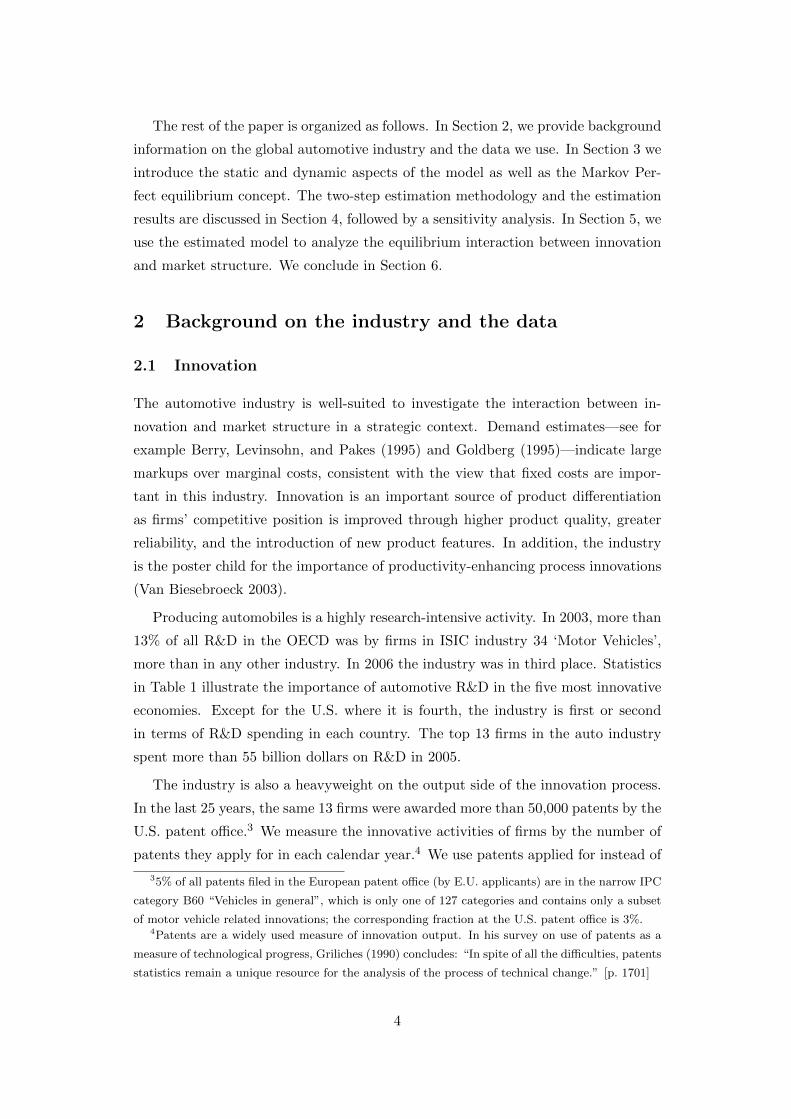
Producing automobiles is a highly research-intensive activity. In 2003, more than
13% of all R&D in the OECD was by firms in ISIC industry 34 ‘Motor Vehicles’,
more than in any other industry. In 2006 the industry was in third place. Statistics
in Table 1 illustrate the importance of automotive R&D in the five most innovative
economies. Except for the U.S. where it is fourth, the industry is first or second
in terms of R&D spending in each country. The top 13 firms in the auto industry
spent more than 55 billion dollars on R&D in 2005.
The industry is also a heavyweight on the output side of the innovation process.
In the last 25 years, the same 13 firms were awarded more than 50,000 patents by the
U.S. patent office.3 We measure the innovative activities of firms by the number of
patents they apply for in each calendar year.4 We use patents applied for instead of
35% of all patents filed in the European patent office (by E.U. applicants) are in the narrow IPC
category B60 “Vehicles in general”, which is only one of 127 categories and contains only a subset
of motor vehicle related innovations; the corresponding fraction at the U.S. patent office is 3%.4Patents are a widely used measure of innovation output. In his survey on use of patents as a
measure of technological progress, Griliches (1990) concludes: “In spite of all the difficulties, patents
statistics remain a unique resource for the analysis of the process of technical change.” [p. 1701]
4
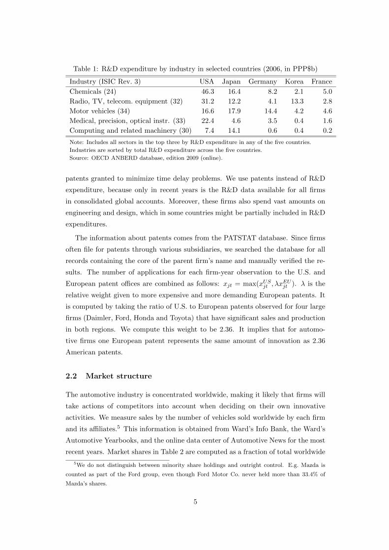
Table 1: R&D expenditure by industry in selected countries (2006, in PPP$b)
Industry (ISIC Rev. 3) USA Japan Germany Korea France
Chemicals (24) 46.3 16.4 8.2 2.1 5.0
Radio, TV, telecom. equipment (32) 31.2 12.2 4.1 13.3 2.8
Motor vehicles (34) 16.6 17.9 14.4 4.2 4.6
Medical, precision, optical instr. (33) 22.4 4.6 3.5 0.4 1.6
Computing and related machinery (30) 7.4 14.1 0.6 0.4 0.2
Note: Includes all sectors in the top three by R&D expenditure in any of the five countries.
Industries are sorted by total R&D expenditure across the five countries.
Source: OECD ANBERD database, edition 2009 (online).
patents granted to minimize time delay problems. We use patents instead of R&D
expenditure, because only in recent years is the R&D data available for all firms
in consolidated global accounts. Moreover, these firms also spend vast amounts on
engineering and design, which in some countries might be partially included in R&D
expenditures.
The information about patents comes from the PATSTAT database. Since firms
often file for patents through various subsidiaries, we searched the database for all
records containing the core of the parent firm’s name and manually verified the re-
sults. The number of applications for each firm-year observation to the U.S. and
European patent offices are combined as follows: xjt = max(xUSjt , λxEUjt ). λ is the
relative weight given to more expensive and more demanding European patents. It
is computed by taking the ratio of U.S. to European patents observed for four large
firms (Daimler, Ford, Honda and Toyota) that have significant sales and production
in both regions. We compute this weight to be 2.36. It implies that for automo-
tive firms one European patent represents the same amount of innovation as 2.36
American patents.
2.2 Market structure
The automotive industry is concentrated worldwide, making it likely that firms will
take actions of competitors into account when deciding on their own innovative
activities. We measure sales by the number of vehicles sold worldwide by each firm
and its affiliates.5 This information is obtained from Ward’s Info Bank, the Ward’s
Automotive Yearbooks, and the online data center of Automotive News for the most
recent years. Market shares in Table 2 are computed as a fraction of total worldwide
5We do not distinguish between minority share holdings and outright control. E.g. Mazda is
counted as part of the Ford group, even though Ford Motor Co. never held more than 33.4% of
Mazda’s shares.
5
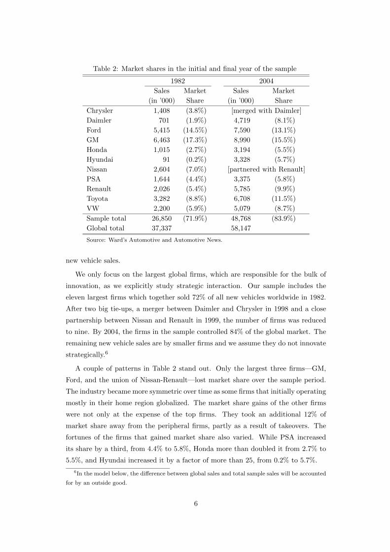
Table 2: Market shares in the initial and final year of the sample
1982 2004
Sales Market Sales Market
(in ’000) Share (in ’000) Share
Chrysler 1,408 (3.8%) [merged with Daimler]
Daimler 701 (1.9%) 4,719 (8.1%)
Ford 5,415 (14.5%) 7,590 (13.1%)
GM 6,463 (17.3%) 8,990 (15.5%)
Honda 1,015 (2.7%) 3,194 (5.5%)
Hyundai 91 (0.2%) 3,328 (5.7%)
Nissan 2,604 (7.0%) [partnered with Renault]
PSA 1,644 (4.4%) 3,375 (5.8%)
Renault 2,026 (5.4%) 5,785 (9.9%)
Toyota 3,282 (8.8%) 6,708 (11.5%)
VW 2,200 (5.9%) 5,079 (8.7%)
Sample total 26,850 (71.9%) 48,768 (83.9%)
Global total 37,337 58,147
Source: Ward’s Automotive and Automotive News.
new vehicle sales.
We only focus on the largest global firms, which are responsible for the bulk of
innovation, as we explicitly study strategic interaction. Our sample includes the
eleven largest firms which together sold 72% of all new vehicles worldwide in 1982.
After two big tie-ups, a merger between Daimler and Chrysler in 1998 and a close
partnership between Nissan and Renault in 1999, the number of firms was reduced
to nine. By 2004, the firms in the sample controlled 84% of the global market. The
remaining new vehicle sales are by smaller firms and we assume they do not innovate
strategically.6
A couple of patterns in Table 2 stand out. Only the largest three firms—GM,
Ford, and the union of Nissan-Renault—lost market share over the sample period.
The industry became more symmetric over time as some firms that initially operating
mostly in their home region globalized. The market share gains of the other firms
were not only at the expense of the top firms. They took an additional 12% of
market share away from the peripheral firms, partly as a result of takeovers. The
fortunes of the firms that gained market share also varied. While PSA increased
its share by a third, from 4.4% to 5.8%, Honda more than doubled it from 2.7% to
5.5%, and Hyundai increased it by a factor of more than 25, from 0.2% to 5.7%.
6In the model below, the difference between global sales and total sample sales will be accounted
for by an outside good.
6
Table 3: Summary statistics
Variable Mean S.D. 10th pctile 90th pctile
Patents 311 268 56 769
Sales (in thousands) 3,653 2,439 900 7,866
Log price (reference firm = 0) -0.03 0.13 -0.19 0.19
Efficiency (reference firm = 0) -1.53 0.97 -2.35 0.48
Note: The number of observations for each variable is 240.
Again because of our focus on strategic interaction in the global automotive
industry, we abstract from the various vehicle models sold by each firm. Instead,
we assume a ‘composite’ model and construct a price for it by estimating a hedonic
price regression. Pooling all available models in a market over the sample period,
we regress the list price in logarithm on a rich set of vehicle characteristics—see
Goldberg and Verboven (2001) for an example. We include a full set of firm-year
interaction dummies and the coefficients on these capture the relative price for each
firm in each year.
This price is relative to the average price charged by a set of peripheral firms,
which are included in the difference between sample and total market in Table 2. It
measures what consumers are willing to pay for a particular firm’s vehicle compared
to a peripheral vehicle with the same characteristics. We estimate this hedonic
regression separately for the U.S. passenger vehicle market, and jointly for five E.U.
countries.7 The (sales) weighted average of a firm’s price in the two markets is its
global price, normalized to zero for the peripheral firms in each year.
The last piece of information we will need to estimate our dynamic model is
the state variable, firm efficiency or product quality. We do not use independent
information for this, but use the residual from a transformed demand equation, the
ξj term in Berry (1994). This measure includes everything that affects a firm’s
market share except the observed vehicle characteristics and prices. It is observed
by all firms in the industry, but not by the econometrician. Most importantly for
our purpose, we hypothesize that its evolution is influenced by innovation.
Summary statistics for the four variables that enter the model are reported in
Table 3. Recall that the sample contains eleven firms over 23 years (1982–2004).
All firms in the sample are very innovative, applying for an average of 311 patents
per year. The standard deviation of 268 suggests that there is a lot of variation
in innovative activities. Average annual sales in the sample is 3.7 million vehicles,
7We have updated the data sets in Petrin (2002) and Goldberg and Verboven (2001) to 2004
using information from JATO Dynamics.
7
500
1000
1500
2000
300
400
500
600
1316192225 1316192225
Total number of patents Patents by revenue (bil. $)
Number of active firms
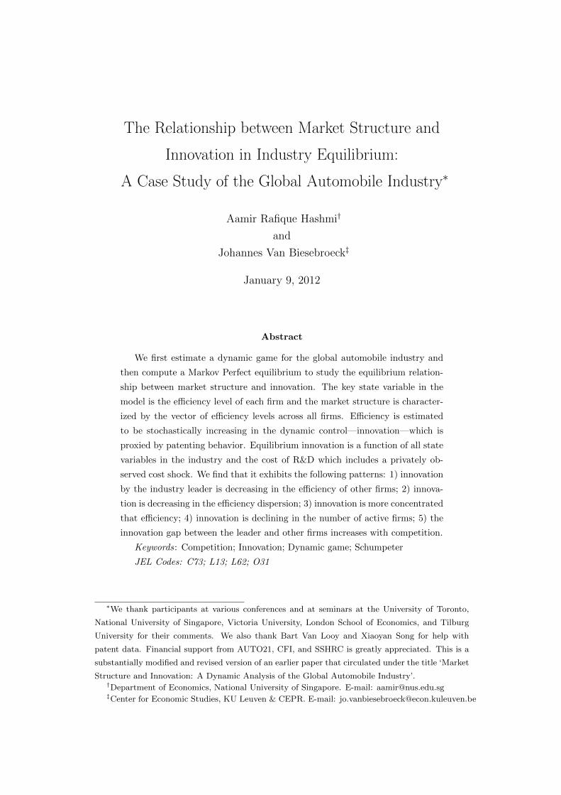
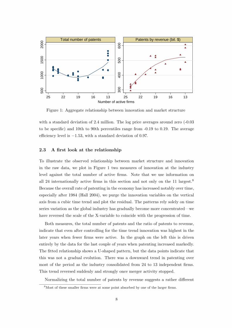
Figure 1: Aggregate relationship between innovation and market structure
with a standard deviation of 2.4 million. The log price averages around zero (-0.03
to be specific) and 10th to 90th percentiles range from -0.19 to 0.19. The average
efficiency level is −1.53, with a standard deviation of 0.97.
2.3 A first look at the relationship
To illustrate the observed relationship between market structure and innovation
in the raw data, we plot in Figure 1 two measures of innovation at the industry
level against the total number of active firms. Note that we use information on
all 24 internationally active firms in this section and not only on the 11 largest.8
Because the overall rate of patenting in the economy has increased notably over time,
especially after 1984 (Hall 2004), we purge the innovation variables on the vertical
axis from a cubic time trend and plot the residual. The patterns rely solely on time
series variation as the global industry has gradually become more concentrated—we
have reversed the scale of the X-variable to coincide with the progression of time.
Both measures, the total number of patents and the ratio of patents to revenue,
indicate that even after controlling for the time trend innovation was highest in the
later years when fewer firms were active. In the graph on the left this is driven
entirely by the data for the last couple of years when patenting increased markedly.
The fitted relationship shows a U-shaped pattern, but the data points indicate that
this was not a gradual evolution. There was a downward trend in patenting over
most of the period as the industry consolidated from 24 to 13 independent firms.
This trend reversed suddenly and strongly once merger activity stopped.
Normalizing the total number of patents by revenue suggests a rather different
8Most of these smaller firms were at some point absorbed by one of the larger firms.
8
050
010
00
0 50 100 0 50 100
1982 2004
New patents applied fitted values: entire periodfitted values: year by year
Revenue
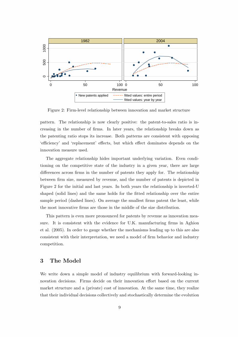
Figure 2: Firm-level relationship between innovation and market structure
pattern. The relationship is now clearly positive: the patent-to-sales ratio is in-
creasing in the number of firms. In later years, the relationship breaks down as
the patenting ratio stops its increase. Both patterns are consistent with opposing
‘efficiency’ and ‘replacement’ effects, but which effect dominates depends on the
innovation measure used.
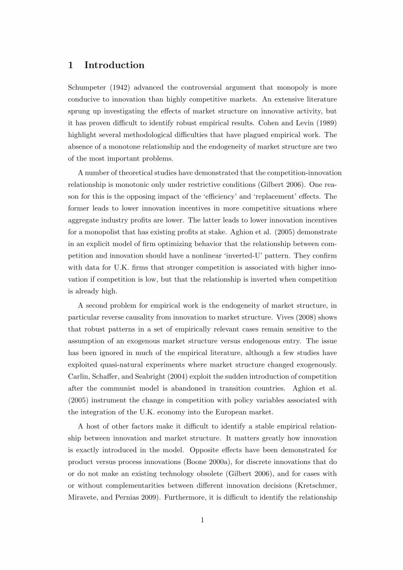
The aggregate relationship hides important underlying variation. Even condi-
tioning on the competitive state of the industry in a given year, there are large
differences across firms in the number of patents they apply for. The relationship
between firm size, measured by revenue, and the number of patents is depicted in
Figure 2 for the initial and last years. In both years the relationship is inverted-U
shaped (solid lines) and the same holds for the fitted relationship over the entire
sample period (dashed lines). On average the smallest firms patent the least, while
the most innovative firms are those in the middle of the size distribution.
This pattern is even more pronounced for patents by revenue as innovation mea-
sure. It is consistent with the evidence for U.K. manufacturing firms in Aghion
et al. (2005). In order to gauge whether the mechanisms leading up to this are also
consistent with their interpretation, we need a model of firm behavior and industry
competition.
3 The Model
We write down a simple model of industry equilibrium with forward-looking in-
novation decisions. Firms decide on their innovation effort based on the current
market structure and a (private) cost of innovation. At the same time, they realize
that their individual decisions collectively and stochastically determine the evolution
9
of the market structure. Our modeling strategy follows Ericson and Pakes (1995)
except for the absence of entry and exit which have not been important in this
industry.
Time is discrete. There are n firms in the industry, each producing a single dif-
ferentiated product. Firms are heterogenous with respect to their relative efficiency
level, ξj ∈ Ξ. At the beginning of each period, firms observe the full state vector for
the industry, their own cost of innovation, and they decide on price and investment
in R&D. While price-setting can be thought of as the equilibrium outcome of a static
Bertrand-Nash game, the investment decisions are the outcome of a dynamic game
of incomplete information.
3.1 The Static Problem
Prices influence current profits, but have no effect on the future. They are chosen
conditioning on the industry state vector and in equilibrium no firm should be willing
to deviate unilaterally. The outcome from the static problem is a mapping from all
possible industry states to a vector of profit levels for each firm under optimally
chosen equilibrium prices.
The demand system is derived from a discrete choice model of individual con-
sumer behavior, following Berry, Levinsohn, and Pakes (1995) and many others
studying the automobile industry. Vehicles differ in quality, ξ, which is observable
to all firms and consumers, but not to the econometrician. There are m consumers
in the market and each buys one vehicle. The utility for consumer i from buying ve-
hicle j depends on its quality, its price and the consumer’s idiosyncratic preferences
as follows
uij = θp log(pj) + ξj + εij , i = 1, . . . ,m, j = 1, . . . , n. (1)
θp is the price elasticity of demand.9 The price of vehicle j incorporates an adjust-
ment for a set of vehicle characteristics as described in the data section. In addition
to the n firms that innovate and price strategically and are the focus of our study,
there are a number of peripheral firms. We normalize the consumer’s utility from
buying a vehicle from a peripheral firm, the outside good, to zero.
If we assume that the idiosyncratic utility εij is i.i.d. extreme value distributed,
9We do not use a random coefficients model because our main focus is on innovation and not on
substitution patterns or on consumer heterogeneity beyond what is implied by εij .
10
we obtain the following expected market share for firm j:10
σj(ξj , ξ−j , pj , p−j) =exp(θp log(pj) + ξj)
1 +∑n
k=1 exp(θp log(pk) + ξk), (2)
where p−j is the price vector of all other firms than j in the industry. The expected
demand is simply mσj(·). The demand that each firm faces depends on the full price
vector for all firms, directly through the denominator of (2) and indirectly through
its own price which, in equilibrium, is a function of its rivals’ prices.
Each firm chooses its price taking the industry state and rival prices as given.
The profit maximization problem of firm j is
πj(ξj , ξ−j , p−j ,m|θp, θc) = maxpj{pj − µj(ξj |θc)}mσj(ξj , ξ−j , pj , p−j |θp).
µj is the marginal cost of firm j and it might vary with the relative efficiency level.
This allows for higher vehicle quality translating in higher costs, but also for cost-
reducing process innovations. θc are the parameters in the marginal cost function.
The first order condition for firm j, after some simplification, is
{pj − µj(·)} {1− σj(·)} θp + pj = 0. (3)
With n active firms, we have to solve n such first order conditions simultaneously
to obtain the equilibrium price vector {p∗j , p∗−j}. Existence and uniqueness of equi-
librium in this context is proved by Caplin and Nalebuff (1991). The equilibrium
profits are then given directly by
π∗j (ξj , ξ−j ,m|θp, θc) = {p∗j − µj(ξj |θc)}mσj(ξj , ξ−j , p∗j , p∗−j |θp). (4)
Once the functional forms and parameter values of the demand and cost functions
are known, the vector of π∗ values for all firms can be calculated for any state of the
industry using equation (4).
3.2 The Dynamic Problem
The optimal innovation decision is a dynamic problem that generates an evolution
for the firm’s state variable. We now have to be more specific on the domain Ξ for ξ.
It is defined by specifying lower and upper bounds and discretizing the intermediate
range of possible values in steps of ∆ξ. As a result, Ξ = {ξmin, ξmin + ∆ξ, · · · , ξmax−∆ξ, ξmax}. Recall that ξj is the relative efficiency of firm j, defined by normalizing
10Anderson, de Palma, and Thisse (1992, p. 136) illustrate how the CES demand system can
equivalently be motivated using the representative consumer framework.
11
the absolute efficiency level by the average efficiency of a set of peripheral firms.
The benefit of this formulation is that ξj is naturally bounded.
Firms also differ in their cost of R&D, which is the sum of a common part that is a
function of R&D expenditure xj and a private shock νj ∈ R that is i.i.d. across firms
and over time and only observed by firm j. The state vector for firm j is then given
by {ξ1, · · · , ξj , · · · , ξn, νj}, which we write in short as sj = {ξj , ξ−j , νj}.11 These
random shocks perform the same function as the choice-specific state variables in
Rust (1987) or Gowrisankaran et al. (2009). They make sure that each investment
choice has positive probability.
Investment in R&D is a strategic and dynamic decision, chosen each period based
on the expected value of future profit streams. The problem is recursive and can be
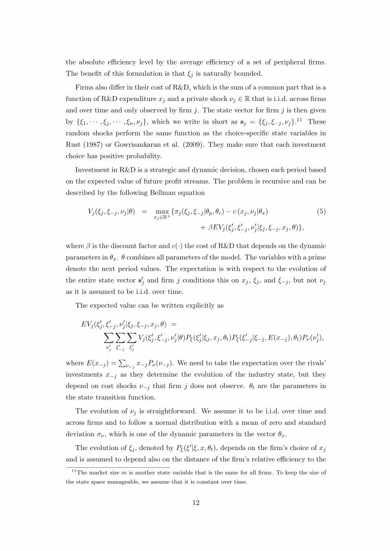
described by the following Bellman equation
Vj(ξj , ξ−j , νj |θ) = maxxj∈R+
{πj(ξj , ξ−j |θp, θc)− c (xj , νj |θx) (5)
+ βEVj(ξ′j , ξ′−j , ν
′j |ξj , ξ−j , xj , θ)},
where β is the discount factor and c(·) the cost of R&D that depends on the dynamic
parameters in θx. θ combines all parameters of the model. The variables with a prime
denote the next period values. The expectation is with respect to the evolution of
the entire state vector s′j and firm j conditions this on xj , ξj , and ξ−j , but not νj
as it is assumed to be i.i.d. over time.
The expected value can be written explicitly as
EVj(ξ′j , ξ′−j , ν
′j |ξj , ξ−j , xj , θ) =∑
ν′j
∑ξ′−j
∑ξ′j
Vj(ξ′j , ξ′−j , ν
′j |θ)Pξ(ξ′j |ξj , xj , θt)Pξ(ξ′−j |ξ−j , E(x−j), θt)Pν(ν ′j),
where E(x−j) =∑
ν−jx−jPν(ν−j). We need to take the expectation over the rivals’
investments x−j as they determine the evolution of the industry state, but they
depend on cost shocks ν−j that firm j does not observe. θt are the parameters in
the state transition function.
The evolution of νj is straightforward. We assume it to be i.i.d. over time and
across firms and to follow a normal distribution with a mean of zero and standard
deviation σν , which is one of the dynamic parameters in the vector θx.
The evolution of ξj , denoted by Pξ(ξ′|ξ, x, θt), depends on the firm’s choice of xj
and is assumed to depend also on the distance of the firm’s relative efficiency to the
11The market size m is another state variable that is the same for all firms. To keep the size of
the state space manageable, we assume that it is constant over time.
12
frontier ξmax.12
We follow Ericson and Pakes (1995) and assume that next period’s efficiency
level can only take three possible values if current efficiency is ξj : (ξj + ∆ξ), ξj , or
(ξj−∆ξ). On the discretized domain, efficiency can increase or decrease by one step
or stay the same. The probability distribution over these possible future states is
given by the triplet{pU , pS , pD
}, which are defined as
pU = Pr(ξ′j = ξj + ∆ξ | ξj
)pS = Pr
(ξ′j = ξj | ξj
)pD = Pr
(ξ′j = ξj −∆ξ | ξj
).
(6)
The functional forms for the transition probabilities will incorporate that the firm
cannot move up anymore when it is at ξmax or down when it is at ξmin.
The solution to (5) is a strategy profile xj = χj(ξj , ξ−j , νj |χ−j). The Markov
Perfect Equilibrium (MPE) of the game is a strategy profile χ∗j that solves (5)
given that all rivals follow the same equilibrium strategy as firm j. It is given by
χ∗j (ξj , ξ−j , νj |χ∗−j), which we denote for short as X∗(s).
In the estimation of the dynamic parameters θx we exploit the properties of
the equilibrium strategy profile. The estimation approach is described in the next
section, where we also introduce the functional form assumptions for the marginal
costs and the transition probabilities.
4 Estimation Methodology and Results
We need to estimate parameters from four functions: demand (θp), marginal cost
(θc), state transitions (θt), and the cost of R&D (θx). The first two sets of parameters
can be estimated from the specification of the static problem and the third set is
merely a parametric description of the observed process in the data. The major
challenge is to estimate the dynamic parameters in the cost of R&D function. With
nine to eleven firms in the industry, the brute force method of computing the Markov
Perfect Equilibrium (MPE) and matching predicted to observed innovation decisions
is computationally infeasible.
12This assumption is supported by the data. The following fixed-effects regression characterizes
changes in efficiency,
∆ξjt = −0.28(0.10)
+ 0.13(0.09)
xjt−1 − 0.13(0.03)
ξjt−1 + γ̂j .
Innovation has a positive effect on the change in efficiency, but a higher level of initial efficiency
makes it harder to improve further.
13
Recently, a number of alternative approaches have been developed that do not
require the calculation of the equilibrium of the game. As observed investment
decisions are equilibrium outcomes, they are used directly to characterize the policy
function and the state transition function (non)parametrically.13
We adopt the two-step estimator of Bajari, Benkard, and Levin (2007) as it is
directly applicable to our situation with a continuous choice variable.14 In the first
step, state transition probabilities and the equilibrium policy functions are combined
with the estimates of the period profit function to obtain numerical estimates of the
value function by forward-simulation. In the second step, the dynamic parameters
are chosen to minimize the deviations from equilibrium conditions, which occur when
the value function is higher under policies that differ from the optimal policies.
We present benchmark estimates and some sensitivity checks immediately follow-
ing the discussion of the estimation methodology for the different elements of the
model.
4.1 Step 1
4.1.1 Demand and Cost Parameters
The demand side in our model is static and we can follow Berry (1994) to write the
log market share of firm j relative to a base firm as15
log[σj(·)/σ0(·)] = θp log[pj/p0] + [ξj − ξ0].
This can be estimated using the observed market shares and price data. The relative
efficiency levels of all firms are then simply the residuals from the demand equation.
Consistent estimation requires that we account for the endogeneity of prices as firms
use unobserved vehicle quality in their pricing decisions. In particular, we expect
the price coefficient to be biased upward if we estimate with ordinary least squares.
The usual instruments in this context are the product characteristics of rival firms,
see for example Berry et al. (1995). In our case, we do not have any characteristics in
the demand equation, as they have already been accounted for in the construction of
the price series. However, lagged patent activity by rival firms should be correlated
with the quality of their current products and thus be correlated with a competitor
13While this approach is widely used in single agent dynamic problems since Hotz and Miller
(1993), in a dynamic game context the assumption is less innocuous due to the possibility of
multiple equilibria, see Doraszelski and Pakes (2007).14Alternative approaches that avoid computing the MPE at each iteration include Aguirregabiria
and Mira (2007) and Pakes, Ostrovsky, and Berry (2007).15All estimators in Step 1 pool data across all years; time subscripts are omitted.
14
firm’s price. We also include firm-fixed effects in the regression, which already absorb
much of the endogeneity as unobserved product quality varies a lot more between
firms than over time. The fixed effects are added again to calculate the ξj series.
Finally, we perform a sensitivity check for the estimation of the dynamic parameters
by selecting a higher and lower price elasticity parameter than the one we estimate.
If marginal costs are assumed constant, the demand function can be estimate
alone. If marginal cost varies with a firm’s efficiency level, it is estimated jointly
with the first order condition for price setting to recover both sets of coefficients. We
use the following specification for the marginal cost function, where the coefficient
on the quadratic term can be fixed to zero or estimated freely:
µj/µ0 = θc0 + θc1ξ̃j + θc2ξ̃2j + εmcj (7)
with ξ̃j = exp(ξj − ξ0).
The estimates for the three different specifications of marginal cost together with
the corresponding price elasticity estimates are reported in Table 4. Price enters
negatively and significantly in each case. Given the log(p) in the indirect utility
function, we are estimating a CES demand model and the coefficient on price directly
gives the price elasticity of demand. Joint estimation of the demand with the first
order condition guarantees an elasticity above unity, but we find this holds even when
demand is estimated separately. Weak instruments or controlling imperfectly for the
product characteristics in the hedonic price regression would lead to an upwardly
biased price coefficient. Both issues do not appear to be problematic.
The estimates range between -3.9 and -2.5, which tends to be lower in absolute
value than the average elasticities that in studies using model-level data. This is
consistent with the more aggregate product definition as the residual demand for a
firm should be less elastic than for an individual model. The implied price-marginal
cost markups are correspondingly lower. Again, this is reasonable because at the
firm level more costs will be variable than at the model level.
The relationship between marginal cost and the unobserved quality term is nega-
tive, in both the linear and quadratic cases.16 It is counterintuitive that firms seem
to be able to produce higher quality vehicles at lower costs. It is therefore better
not to think of ξ as just product quality, but any unobservable that makes the firm
achieve high sales. It is not surprising that factors that make a firm succeed in the
marketplace are correlated with factors that make it produce efficiently.
16The same holds if we specify the logarithm rather than the level of marginal cost as the linear
function in equation (7).
15
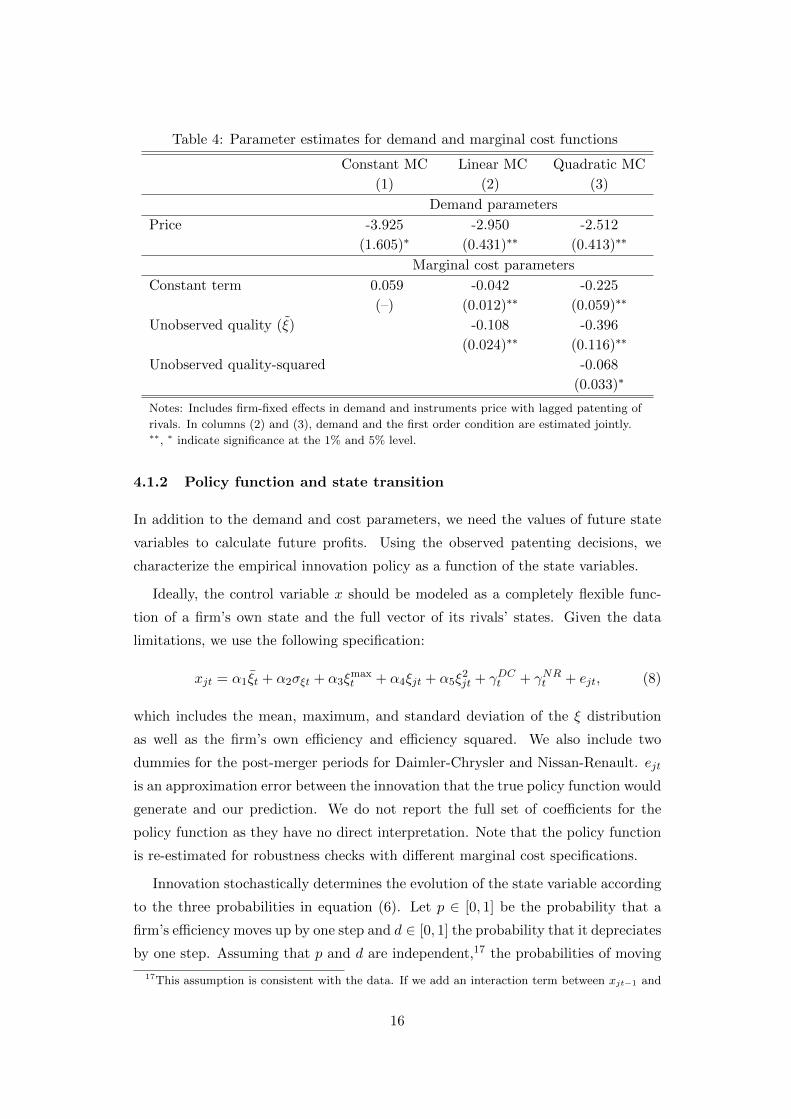
Table 4: Parameter estimates for demand and marginal cost functions
Constant MC Linear MC Quadratic MC
(1) (2) (3)
Demand parameters
Price -3.925 -2.950 -2.512
(1.605)∗ (0.431)∗∗ (0.413)∗∗
Marginal cost parameters
Constant term 0.059 -0.042 -0.225
(–) (0.012)∗∗ (0.059)∗∗
Unobserved quality (ξ̃) -0.108 -0.396
(0.024)∗∗ (0.116)∗∗
Unobserved quality-squared -0.068
(0.033)∗
Notes: Includes firm-fixed effects in demand and instruments price with lagged patenting of
rivals. In columns (2) and (3), demand and the first order condition are estimated jointly.∗∗, ∗ indicate significance at the 1% and 5% level.
4.1.2 Policy function and state transition
In addition to the demand and cost parameters, we need the values of future state
variables to calculate future profits. Using the observed patenting decisions, we
characterize the empirical innovation policy as a function of the state variables.
Ideally, the control variable x should be modeled as a completely flexible func-
tion of a firm’s own state and the full vector of its rivals’ states. Given the data
limitations, we use the following specification:
xjt = α1ξ̄t + α2σξt + α3ξmaxt + α4ξjt + α5ξ
2jt + γDCt + γNRt + ejt, (8)
which includes the mean, maximum, and standard deviation of the ξ distribution
as well as the firm’s own efficiency and efficiency squared. We also include two
dummies for the post-merger periods for Daimler-Chrysler and Nissan-Renault. ejt
is an approximation error between the innovation that the true policy function would
generate and our prediction. We do not report the full set of coefficients for the
policy function as they have no direct interpretation. Note that the policy function
is re-estimated for robustness checks with different marginal cost specifications.
Innovation stochastically determines the evolution of the state variable according
to the three probabilities in equation (6). Let p ∈ [0, 1] be the probability that a
firm’s efficiency moves up by one step and d ∈ [0, 1] the probability that it depreciates
by one step. Assuming that p and d are independent,17 the probabilities of moving
17This assumption is consistent with the data. If we add an interaction term between xjt−1 and
16
up, staying put, or moving down are
pU = p (1− d)
pS = pd+ (1− p)(1− d)
pD = (1− p)d,
and we use the following parameterizations for p and d:
p = 1− exp(−θt1 − θt2x),
d = exp
(−θt3
ξmax − ξξmax − ξmin
).
This specification has several attractive properties. First, if θt2 > 0 patenting
increase the probability that efficiency increases. Second, if innovation goes to in-
finity, efficiency increases almost surely. Third, even if a firm does not innovate
there is some positive probability that its efficiency improves. Fourth, if θt3 > 0, the
probability that efficiency depreciates is inversely related to the distance from the
frontier.
Together these probabilities fully define the transition function Pξ(ξ′|ξ, x). They
also imply that when a firm is at maximum efficiency, the probability of a further
increases is zero because d = 1. At the other extreme, when the firm is at the
minimum level of efficiency, it does not hold automatically that pD = 0 and we need
to enforce this. If ξ = ξmin, we assume that pD = 0 and adjust pS to equal 1− pU .
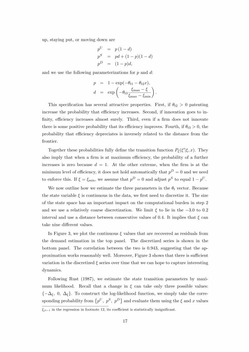
We now outline how we estimate the three parameters in the θt vector. Because
the state variable ξ is continuous in the data, we first need to discretize it. The size
of the state space has an important impact on the computational burden in step 2
and we use a relatively coarse discretization. We limit ξ to lie in the −3.0 to 0.2
interval and use a distance between consecutive values of 0.4. It implies that ξ can
take nine different values.
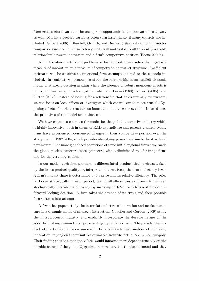
In Figure 3, we plot the continuous ξ values that are recovered as residuals from
the demand estimation in the top panel. The discretized series is shown in the
bottom panel. The correlation between the two is 0.943, suggesting that the ap-
proximation works reasonably well. Moreover, Figure 3 shows that there is sufficient
variation in the discretized ξ series over time that we can hope to capture interesting
dynamics.
Following Rust (1987), we estimate the state transition parameters by maxi-
mum likelihood. Recall that a change in ξ can take only three possible values:
{−∆ξ, 0, ∆ξ}. To construct the log-likelihood function, we simply take the corre-
sponding probability from{pU , pS , pD
}and evaluate them using the ξ and x values
ξjt−1 in the regression in footnote 12, its coefficient is statistically insignificant.
17
1982 1984 1986 1988 1990 1992 1994 1996 1998 2000 2002 2004−2.5
−2
−1.5
−1
−0.5
0
Evolution of Continuous ξ
Year
ξ
1982 1984 1986 1988 1990 1992 1994 1996 1998 2000 2002 2004−2.5
−2
−1.5
−1
−0.5
0
Evolution of Discrete ξ (∆ ξ = 0.2)
Year
ξ
1982 1984 1986 1988 1990 1992 1994 1996 1998 2000 2002 2004−2.5
−2
−1.5
−1
−0.5
0
Evolution of Discrete ξ (∆ ξ = 0.4)
Year
ξ
1982 1984 1986 1988 1990 1992 1994 1996 1998 2000 2002 2004−2.5
−2
−1.5
−1
−0.5
0
Evolution of Continuous ξ
Year
ξ
1982 1984 1986 1988 1990 1992 1994 1996 1998 2000 2002 2004−2.5
−2
−1.5
−1
−0.5
0
Evolution of Discrete ξ (∆ ξ = 0.2)
Year
ξ
1982 1984 1986 1988 1990 1992 1994 1996 1998 2000 2002 2004−2.5
−2
−1.5
−1
−0.5
0
Evolution of Discrete ξ (∆ ξ = 0.4)
Year
ξ
Figure 3: Evolution of efficiency for selected firms
Note: The top panel shows the estimated (continuous) values for ξ and the bottom panel the
discretized efficiency levels used in the model.
for each observation. The objective function is then the sum of the logarithms of
the relevant probabilities over all observations in the sample.
The parameter estimates for the three specifications for marginal costs are in
Table 5. We faced two problems. First, due to the coarse discretization of ξ, some
of the standard errors are extremely high. With a finer discretization this problem
largely disappears, with t-statistics above 1.5 even for θt3. We use the current point
estimates to reduce the computational burden in the next step.
Second, the parameter estimate for θt2, which captures the impact of innovation
on the probability that efficiency increases, is negative in the third specification,
although it is estimated very imprecisely. It would imply that innovation lowers
the probability of improving efficiency. This problem does not appear when using
18
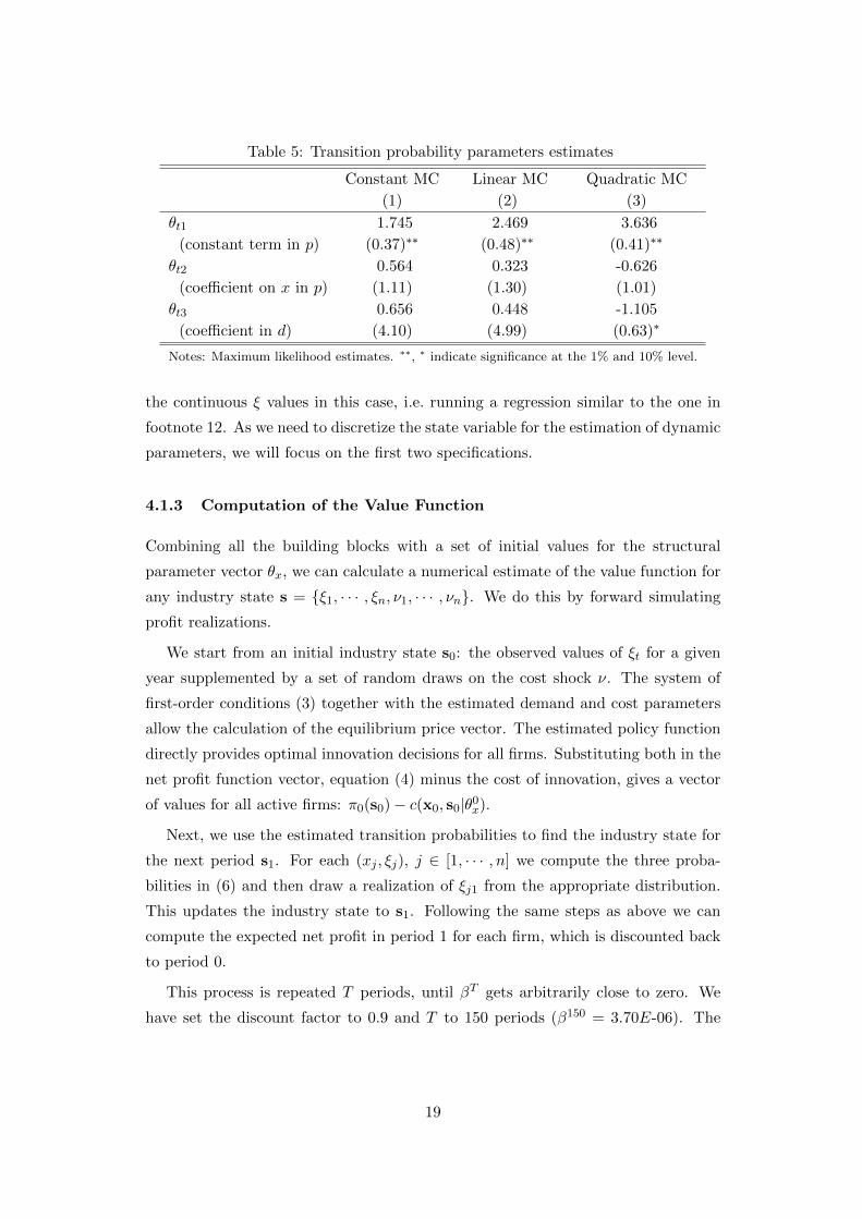
Table 5: Transition probability parameters estimates
Constant MC Linear MC Quadratic MC
(1) (2) (3)
θt1 1.745 2.469 3.636
(constant term in p) (0.37)∗∗ (0.48)∗∗ (0.41)∗∗
θt2 0.564 0.323 -0.626
(coefficient on x in p) (1.11) (1.30) (1.01)
θt3 0.656 0.448 -1.105
(coefficient in d) (4.10) (4.99) (0.63)∗
Notes: Maximum likelihood estimates. ∗∗, ∗ indicate significance at the 1% and 10% level.
the continuous ξ values in this case, i.e. running a regression similar to the one in
footnote 12. As we need to discretize the state variable for the estimation of dynamic
parameters, we will focus on the first two specifications.
4.1.3 Computation of the Value Function
Combining all the building blocks with a set of initial values for the structural
parameter vector θx, we can calculate a numerical estimate of the value function for
any industry state s = {ξ1, · · · , ξn, ν1, · · · , νn}. We do this by forward simulating
profit realizations.
We start from an initial industry state s0: the observed values of ξt for a given
year supplemented by a set of random draws on the cost shock ν. The system of
first-order conditions (3) together with the estimated demand and cost parameters
allow the calculation of the equilibrium price vector. The estimated policy function
directly provides optimal innovation decisions for all firms. Substituting both in the
net profit function vector, equation (4) minus the cost of innovation, gives a vector
of values for all active firms: π0(s0)− c(x0, s0|θ0x).
Next, we use the estimated transition probabilities to find the industry state for
the next period s1. For each (xj , ξj), j ∈ [1, · · · , n] we compute the three proba-
bilities in (6) and then draw a realization of ξj1 from the appropriate distribution.
This updates the industry state to s1. Following the same steps as above we can
compute the expected net profit in period 1 for each firm, which is discounted back
to period 0.
This process is repeated T periods, until βT gets arbitrarily close to zero. We
have set the discount factor to 0.9 and T to 150 periods (β150 = 3.70E-06). The
19
value functions are then simply the present discounted values of these profit streams:
V (s0|θ0x) = E
[T∑t=0
βt[πt(st)− c(xt, st|θ0x
)]
], (9)
where the expectation is over future states. We perform these forward simulations
10, 000 times using different draws for the ν shocks and the realizations of the state
transitions. The average over all simulations is the numerical estimate of V (s0|θ0x)
for starting state s0. We repeat this for all observed industry states by taking each
as the starting state for a separate set of simulations.
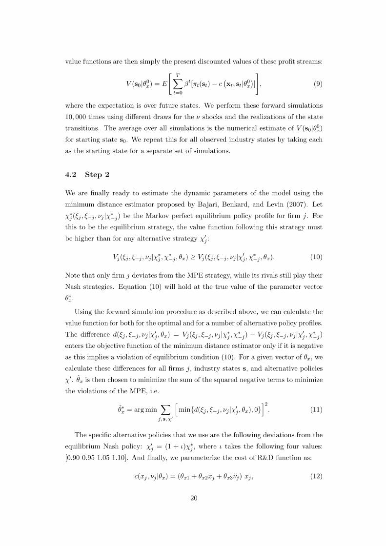
4.2 Step 2
We are finally ready to estimate the dynamic parameters of the model using the
minimum distance estimator proposed by Bajari, Benkard, and Levin (2007). Let
χ∗j (ξj , ξ−j , νj |χ∗−j) be the Markov perfect equilibrium policy profile for firm j. For
this to be the equilibrium strategy, the value function following this strategy must
be higher than for any alternative strategy χ′j :
Vj(ξj , ξ−j , νj |χ∗j , χ∗−j , θx) ≥ Vj(ξj , ξ−j , νj |χ′j , χ∗−j , θx). (10)
Note that only firm j deviates from the MPE strategy, while its rivals still play their
Nash strategies. Equation (10) will hold at the true value of the parameter vector
θ∗x.
Using the forward simulation procedure as described above, we can calculate the
value function for both for the optimal and for a number of alternative policy profiles.
The difference d(ξj , ξ−j , νj |χ′j , θx) = Vj(ξj , ξ−j , νj |χ∗j , χ∗−j) − Vj(ξj , ξ−j , νj |χ′j , χ∗−j)enters the objective function of the minimum distance estimator only if it is negative
as this implies a violation of equilibrium condition (10). For a given vector of θx, we
calculate these differences for all firms j, industry states s, and alternative policies
χ′. θ̂x is then chosen to minimize the sum of the squared negative terms to minimize
the violations of the MPE, i.e.
θ̂∗x = arg min∑j, s, χ′
[min{d(ξj , ξ−j , νj |χ′j , θx), 0}
]2. (11)
The specific alternative policies that we use are the following deviations from the
equilibrium Nash policy: χ′j = (1 + ι)χ∗j , where ι takes the following four values:
[0.90 0.95 1.05 1.10]. And finally, we parameterize the cost of R&D function as:
c(xj , νj |θx) = (θx1 + θx2xj + θx3ν̃j) xj , (12)
20
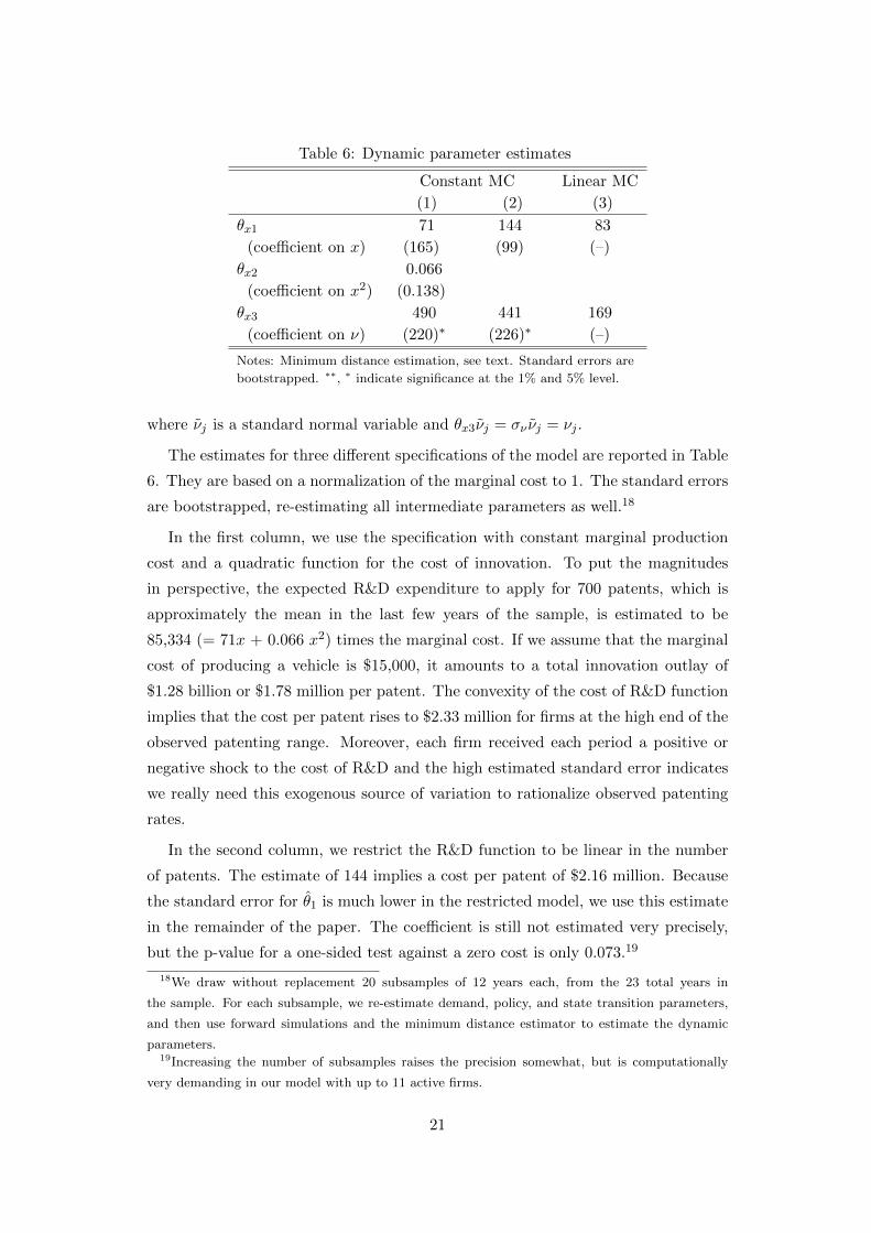
Table 6: Dynamic parameter estimates
Constant MC Linear MC
(1) (2) (3)
θx1 71 144 83
(coefficient on x) (165) (99) (–)
θx2 0.066
(coefficient on x2) (0.138)
θx3 490 441 169
(coefficient on ν) (220)∗ (226)∗ (–)
Notes: Minimum distance estimation, see text. Standard errors are
bootstrapped. ∗∗, ∗ indicate significance at the 1% and 5% level.
where ν̃j is a standard normal variable and θx3ν̃j = σν ν̃j = νj .
The estimates for three different specifications of the model are reported in Table
6. They are based on a normalization of the marginal cost to 1. The standard errors
are bootstrapped, re-estimating all intermediate parameters as well.18
In the first column, we use the specification with constant marginal production
cost and a quadratic function for the cost of innovation. To put the magnitudes
in perspective, the expected R&D expenditure to apply for 700 patents, which is
approximately the mean in the last few years of the sample, is estimated to be
85,334 (= 71x + 0.066 x2) times the marginal cost. If we assume that the marginal
cost of producing a vehicle is $15,000, it amounts to a total innovation outlay of
$1.28 billion or $1.78 million per patent. The convexity of the cost of R&D function
implies that the cost per patent rises to $2.33 million for firms at the high end of the
observed patenting range. Moreover, each firm received each period a positive or
negative shock to the cost of R&D and the high estimated standard error indicates
we really need this exogenous source of variation to rationalize observed patenting
rates.
In the second column, we restrict the R&D function to be linear in the number
of patents. The estimate of 144 implies a cost per patent of $2.16 million. Because
the standard error for θ̂1 is much lower in the restricted model, we use this estimate
in the remainder of the paper. The coefficient is still not estimated very precisely,
but the p-value for a one-sided test against a zero cost is only 0.073.19
18We draw without replacement 20 subsamples of 12 years each, from the 23 total years in
the sample. For each subsample, we re-estimate demand, policy, and state transition parameters,
and then use forward simulations and the minimum distance estimator to estimate the dynamic
parameters.19Increasing the number of subsamples raises the precision somewhat, but is computationally
very demanding in our model with up to 11 active firms.
21
We have investigated the sensitivity of the estimates in column (2) to the price
elasticity of demand, which is a key parameter in the model. It determines not
only how high the price-cost margins and thus profits are, but also how consumers
trade off lower prices and higher quality. Both are key considerations in the firms’
innovation decision. In the benchmark case with constant marginal cost, the price
elasticity was estimated at −3.92. We re-estimate the dynamic parameters when
the elasticity is set to one half and to double the estimated value.
As the price elasticity rises from −1.96, over −3.92, to −7.85, the θ̂1 estimate
falls from 261, to 144, and 114. The intuition is the following. When demand is
less elastic, markups are higher and so are profits from increased sales. In addition,
consumers value a high vehicle quality relatively more than a low price. As a result,
the incentives to innovate are raised and to rationalize the observed number of
patents in the data we need a higher cost of R&D.
At the same time, the θ̂3 estimate for the standard deviation of the shock to
innovation falls from 1059, to 441, and 19. This is the result from an asymmetric
effect of the cost shocks. As we impose that the cost of R&D can never be negative, a
higher standard deviation mainly has an effect on the positive side, i.e. to discourage
innovation. Several firms in the data are observed to innovate less than we would
predict based on the model primitives and the shock rationalizes their behavior.
When the price elasticity is very high, the incentives to innovate in the model are
reduced and we can fit the patenting activity without requiring large variations in
the cost of innovation.
The results reported in the third column of Table 6 allow the marginal production
cost to vary with firm efficiency. Recall that we found marginal costs to be declining
in efficiency in Table 4, but we nevertheless find lower estimates for both θ̂1 and θ̂3,
at 83 and 169. It is counterintuitive that the model comes up with a lower cost of
innovation to match observed rates of patenting when patents have the additional
benefit of lowering production costs. The explanation comes from the differences
in state-transition estimates. The lower estimates for θ̂t2 in the second column of
Table 5 implies that innovation has less of a positive effect on the probability that
efficiency improves in this case. The lower estimate for θ̂t3 implies slower depreciation
of efficiency, further reducing the incentive to innovate. These effects outweigh the
boost in incentives coming from the production costs.
22
5 Market Structure and Innovation
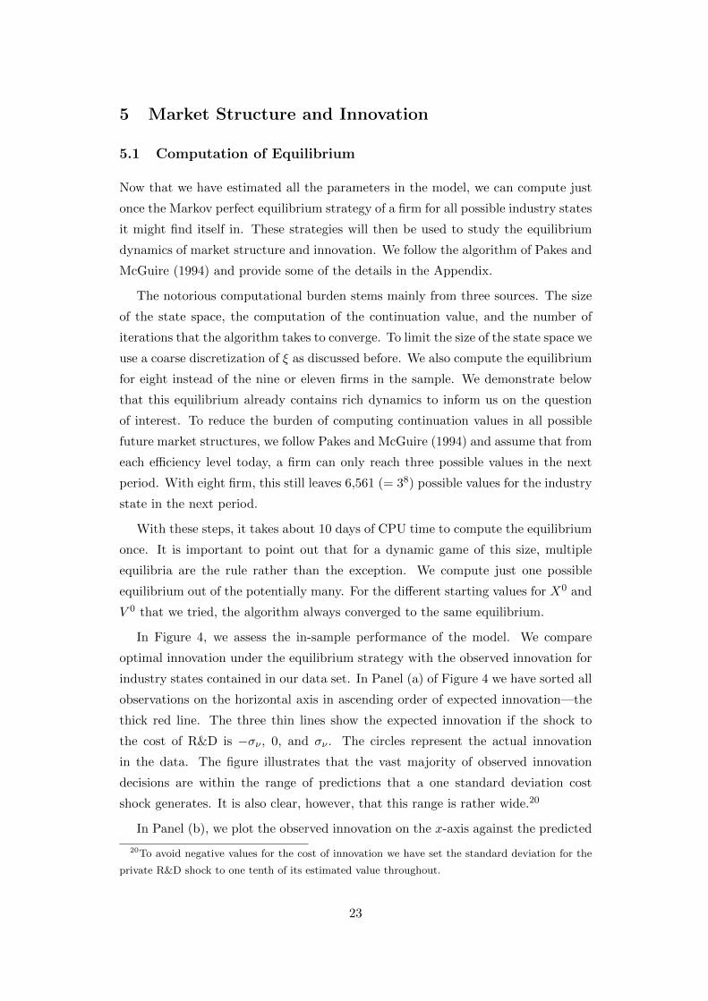
5.1 Computation of Equilibrium
Now that we have estimated all the parameters in the model, we can compute just
once the Markov perfect equilibrium strategy of a firm for all possible industry states
it might find itself in. These strategies will then be used to study the equilibrium
dynamics of market structure and innovation. We follow the algorithm of Pakes and
McGuire (1994) and provide some of the details in the Appendix.
The notorious computational burden stems mainly from three sources. The size
of the state space, the computation of the continuation value, and the number of
iterations that the algorithm takes to converge. To limit the size of the state space we
use a coarse discretization of ξ as discussed before. We also compute the equilibrium
for eight instead of the nine or eleven firms in the sample. We demonstrate below
that this equilibrium already contains rich dynamics to inform us on the question
of interest. To reduce the burden of computing continuation values in all possible
future market structures, we follow Pakes and McGuire (1994) and assume that from
each efficiency level today, a firm can only reach three possible values in the next
period. With eight firm, this still leaves 6,561 (= 38) possible values for the industry
state in the next period.
With these steps, it takes about 10 days of CPU time to compute the equilibrium
once. It is important to point out that for a dynamic game of this size, multiple
equilibria are the rule rather than the exception. We compute just one possible
equilibrium out of the potentially many. For the different starting values for X0 and
V 0 that we tried, the algorithm always converged to the same equilibrium.
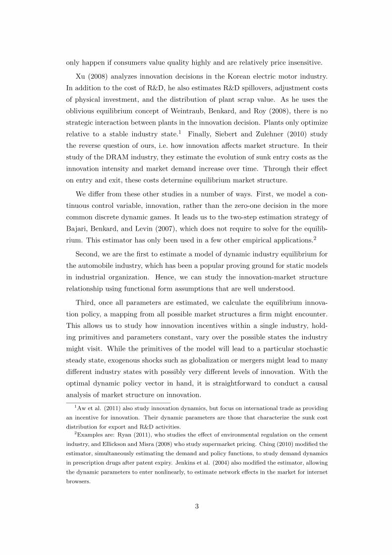
In Figure 4, we assess the in-sample performance of the model. We compare
optimal innovation under the equilibrium strategy with the observed innovation for
industry states contained in our data set. In Panel (a) of Figure 4 we have sorted all
observations on the horizontal axis in ascending order of expected innovation—the
thick red line. The three thin lines show the expected innovation if the shock to
the cost of R&D is −σν , 0, and σν . The circles represent the actual innovation
in the data. The figure illustrates that the vast majority of observed innovation
decisions are within the range of predictions that a one standard deviation cost
shock generates. It is also clear, however, that this range is rather wide.20
In Panel (b), we plot the observed innovation on the x-axis against the predicted
20To avoid negative values for the cost of innovation we have set the standard deviation for the
private R&D shock to one tenth of its estimated value throughout.
23
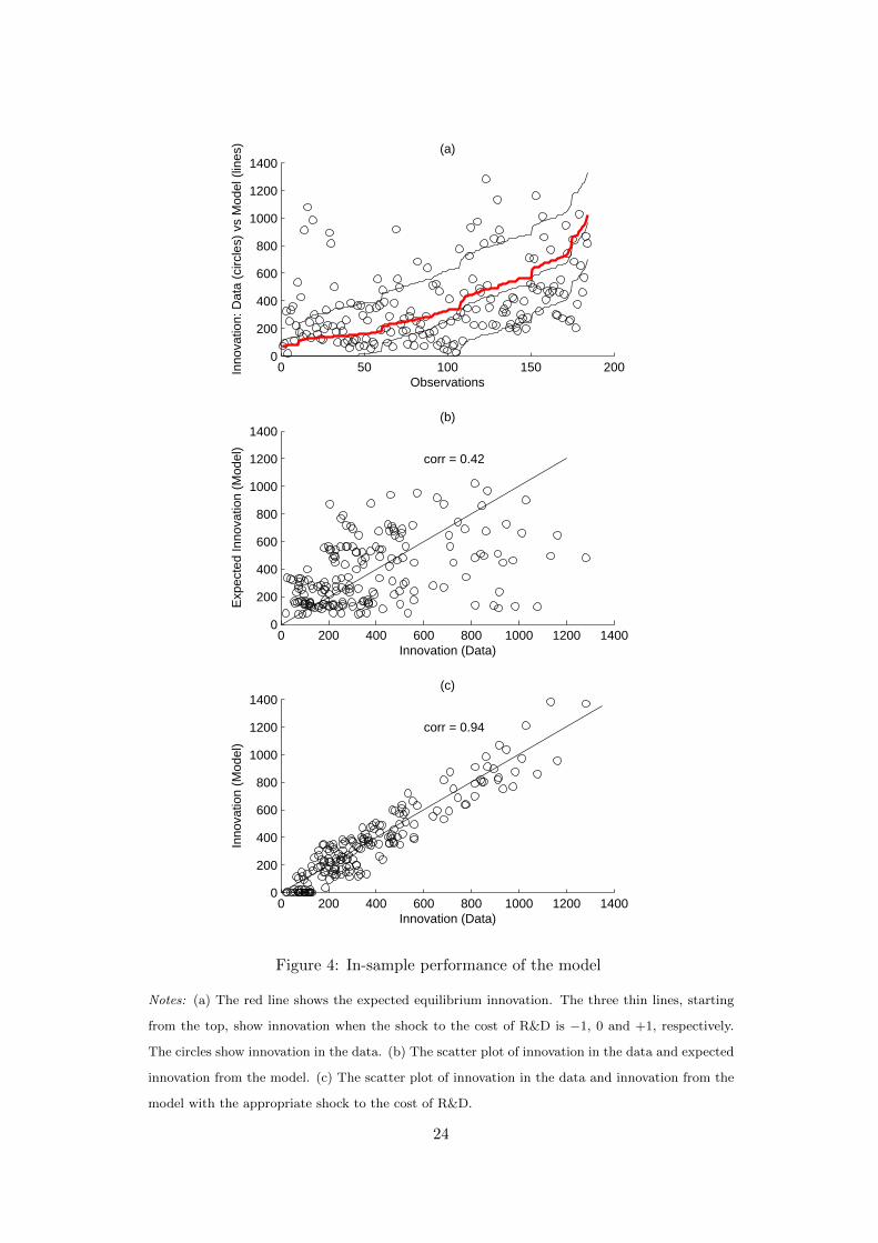
0 50 100 150 2000
200
400
600
800
1000
1200
1400(a)
Observations
Inno
vatio
n: D
ata
(circ
les)
vs
Mod
el (
lines
)
0 200 400 600 800 1000 1200 14000
200
400
600
800
1000
1200
1400(b)
Innovation (Data)
Exp
ecte
d In
nova
tion
(Mod
el)
corr = 0.42
0 200 400 600 800 1000 1200 14000
200
400
600
800
1000
1200
1400(c)
Innovation (Data)
Inno
vatio
n (M
odel
)
corr = 0.94
Figure 4: In-sample performance of the model
Notes: (a) The red line shows the expected equilibrium innovation. The three thin lines, starting
from the top, show innovation when the shock to the cost of R&D is −1, 0 and +1, respectively.
The circles show innovation in the data. (b) The scatter plot of innovation in the data and expected
innovation from the model. (c) The scatter plot of innovation in the data and innovation from the
model with the appropriate shock to the cost of R&D.
24
equilibrium innovation on the y-axis. The correlation is 0.42 and the model only does
a modest job of predicting the data. This should not be surprising as the estimated
importance of the random shock to the cost of R&D was rather large. We allowed
the shock to the cost of R&D to take one of five values: {−2σν ,−σν , 0, σν , 2σν}.Expected innovation is computed by taking the expectation over the equilibrium
innovation for each possible realization of the shock. In Panel (c), we report the
equilibrium innovation when we pick for each observation the value of the shock (out
of the 5 possible values) that minimizes the difference between actual and equilibrium
innovation. The correlation between the actual and equilibrium innovation is now
0.94, illustrating that the model is capable of rationalizing the data quite well.
In Figure A.1 in the Appendix we further illustrate that the calculated optimal
investment policy leads to an evolution of efficiency levels that captures the observed
patterns quite well. Starting from the observed industry state in 1982 for the eight
largest firms, we simulate the industry forward till 2004 one thousand times using
the optimal innovation policy. The average evolution (red lines) track the actual
evolutions (black lines) rather well.21 The average correlation between the actual
and predicted efficiency levels is 0.75.
5.2 Equilibrium Relationship between Market Structure and Inno-
vation
We now turn to the main question that motivated the paper: what is the equilib-
rium relationship between market structure and innovation in the global automobile
industry? We illustrate several patterns by graphing optimal innovation using the
MPE policy vector against specific variations in market structure.
We use the optimal policies that we calculated for all possible market structures
because in the data we only observe a small set of states for the industry. This
is illustrated in Figure A.2 in the Appendix, where we forward simulate the model
using optimal innovation and random draws on the transition process. The figure
shows the average efficiency in the industry for one thousand periods starting from
an initial state where all eight firms have ξj = −0.5. We see that there can be quite
dramatic endogenous changes. For example, in the 30 periods following t = 380, the
average efficiency level increases from close to −1 to almost −0.1. There are several
such episodes and they imply even more dramatic changes at the firm level. We also
see that, despite the sometimes dramatic changes, the industry is in a stochastic
steady state.
21The averaging over different industry realizations has smoothed the predicted evolution.
25
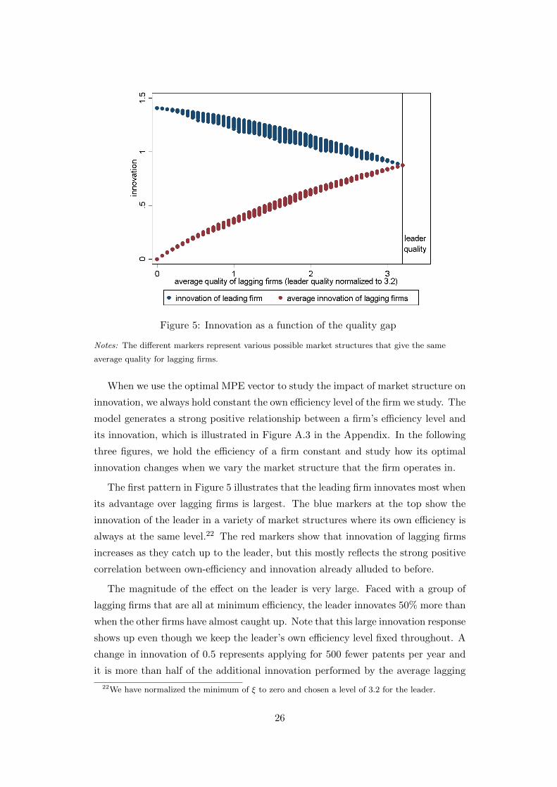
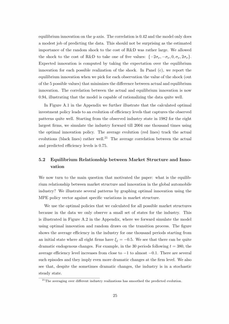
Figure 5: Innovation as a function of the quality gap
Notes: The different markers represent various possible market structures that give the same
average quality for lagging firms.
When we use the optimal MPE vector to study the impact of market structure on
innovation, we always hold constant the own efficiency level of the firm we study. The
model generates a strong positive relationship between a firm’s efficiency level and
its innovation, which is illustrated in Figure A.3 in the Appendix. In the following
three figures, we hold the efficiency of a firm constant and study how its optimal
innovation changes when we vary the market structure that the firm operates in.
The first pattern in Figure 5 illustrates that the leading firm innovates most when
its advantage over lagging firms is largest. The blue markers at the top show the
innovation of the leader in a variety of market structures where its own efficiency is
always at the same level.22 The red markers show that innovation of lagging firms
increases as they catch up to the leader, but this mostly reflects the strong positive
correlation between own-efficiency and innovation already alluded to before.
The magnitude of the effect on the leader is very large. Faced with a group of
lagging firms that are all at minimum efficiency, the leader innovates 50% more than
when the other firms have almost caught up. Note that this large innovation response
shows up even though we keep the leader’s own efficiency level fixed throughout. A
change in innovation of 0.5 represents applying for 500 fewer patents per year and
it is more than half of the additional innovation performed by the average lagging
22We have normalized the minimum of ξ to zero and chosen a level of 3.2 for the leader.
26
Figure 6: Innovation as a function of mean-preserving quality dispersion
firm as its efficiency level is raised over the full range of the state variable.23.
The second pattern in Figure 6 looks at innovation of a firm holding constant
not only its own efficiency level and its relative position in the industry, but also
the average level of efficiency for the industry as a whole. On the horizontal axis we
measure the dispersion of efficiency in the industry, where variation is added in a
mean-preserving way. On the vertical axis we indicate innovation of the middle firm
(green markers), the average innovation for the industry (solid line) and the lowest
and highest industry average innovation across different market structures (dashed
lines).24
The central pattern in this figure is of declining innovation as efficiency becomes
more unequal. The middle firm innovates less when its distance to the industry
leaders grows, even though its own advantage over laggards grows by the same
amount. Average innovation falls as well, which is the result of a concave relationship
between innovation and own efficiency (Figure A.3). As a result, holding total
efficiency for the industry constant, total innovation is maximized when the efficiency
is divided equally among firms.
23Figure A.3 in the Appendix shows that the innovation of a group of symmetric firms grows by
approximately the same amount, from 0.25 to 0.75, if their efficiency level is raised over the full
range of the state variable24We only show market structures where no firm is at zero efficiency as the sudden drop in
innovation at that point would introduce small jumps in the figure.
27
The previous pattern in Figure 5 works against this trend of declining average
innovation with dispersion. Innovation incentives for the leaders get stronger as
their advantage grows, but this effect is not strong enough to overcome the effect
of concavity. It does show up, however, in a less pronounced decline of the average
innovation level compared with the decline for the middle firm.
These same effects also give rise to a positive and more than proportional rela-
tionship between concentration in innovation and in efficiency. When the allocation
of the state variable is more concentrated, innovation is also more concentrated.
The relationship, shown in Figure A.4 in the Appendix, is even steeper than the
45 degree line. A 50% rise in the Herfindahl index for efficiency can double the
Herfindahl index for innovation. At the same time, total innovation for the industry
is a declining function of the concentration in efficiency, in line with the dispersion
results in Figure 6.
Another interesting question is whether industry leaders innovate more than fol-
lowers. However, it is difficult to make such a comparison while holding constant own
efficiency and total efficiency for the industry. The only way to do this is to make
the distribution less dispersed when we consider the leader’s innovation, but Figure
6 already demonstrated that this in itself raises innovation. We made a number of
comparisons for an industry consisting of just three firms and found innovation to
be between 1.1% and 3.3% higher for a leader compared to a follower with the same
efficiency level, when holding total efficiency in the industry constant as well.
We can make similar comparisons to verify whether a firm at the very bottom
innovates more or less than a firm in the middle. Again, the only way to do this
while holding own efficiency and total industry efficiency constant is to make the
distribution less dispersed for the bottom firm. Across several cases, we find that
the bottom firm innovates 0.7% to 4.1% more than the middle firm. These results
suggest that innovation is higher for firms at the very top or bottom than for firms
in the middle, but we cannot rule out entirely that this is the result of efficiency
dispersion rather than the firm’s own position in the industry.
The above results are all for the specification of the model with constant marginal
production costs. The pattern in Figure 5 is similar when we use the model with
marginal production costs declining in efficiency. Only the range of innovation over
different possible market structures is wider, both for the leader and lagging firms.
The pattern in Figure 6 is similar for the middle firm, but the average innovation in
the industry is now increasing in dispersion, see Figure A.5 in the Appendix. The
reason is that the relationship between own-efficiency and innovation is still increas-
ing, but now has an S-shape rather than being concave. It makes the innovation
28
Figure 7: Innovation as a function of the number of firms
boost for the leading firms more important and suggests that in this case aggregate
innovation would be much higher if efficiency were highly asymmetric.25
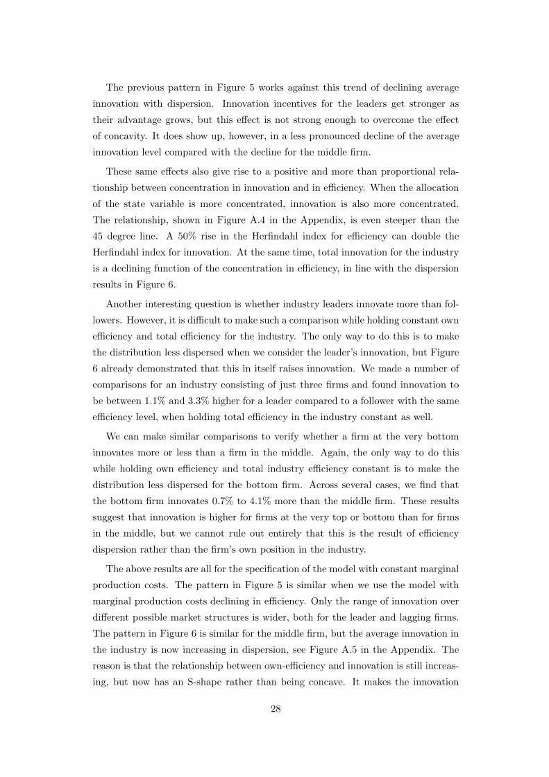
The last pattern in Figure 7 illustrates how innovation changes when the number
of competitors is exogenously increased.26 Again, we hold the relative and absolute
position of a firm constant and plot its optimal level of innovation as we add firms to
the market. Additional firms are always entered at the mean level of efficiency. The
blue circled markers are for a firm that is also at the mean efficiency level, i.e. all
firms in the industry are symmetric in this case. The figure shows a monotonically
declining rate of innovation with competition, consistent with the efficiency effect.
As the number of active firms increases in a market of constant size, profit rates will
go down and innovation incentives with them. Firms do take some market share
away from the outside good, but it is not enough to compensate for the additional
competition. Note that the interpretation here is really the innovation response
to an exogenous change in market structure as we always use the optimal MPE
innovation policy.
The same pattern of declining innovation with competition holds for leading and
lagging firms, but for firms that are ahead of the new entrants the innovation decline
25The same mechanism also leads to higher average innovation for higher levels of the Herfindahl
index in efficiency in this case.26To construct this figure we computed the optimal policy vector for different numbers of active
firms.
29
is much less pronounced. To illustrate this more clearly, we included red lines on
the graph that express innovation of an existing leading or lagging firm relative to
the innovation of firms at average efficiency, either existing or new entrants. The
interpretation of the red lines is that they are the optimal innovation policies of
leaders or laggards, relative to the optimal policies of average firms.
For existing industry leaders, their relative rate of innovation increases strongly
when additional competitors enter the market. A firm with a competitive advantage
will increase its innovation lead over other firms when faced with more competition.
While its absolute level of innovation is declining with entry, it declines much less
than the innovation of other (average) firms. This pattern is in line with the replace-
ment effect. A firm that is innovating to defend its competitive position, increases
the gap with other firms when facing more competition.
6 Concluding remarks
We have accomplished two things. First, we estimated all parameters in a structural
game-theoretic model of strategic, forward-looking, innovating firms for a particular
sector. Second, we calculated the optimal Markov-perfect equilibrium policy for
this game for all possible industry states and used it to investigate how optimal
innovation responds to exogenous changes in market structure.
The structural approach in this paper has a number of advantages over reduced
form approaches that look directly at the relationship between innovation and mar-
ket structure in the data. It allows us to focus on the equilibrium relationships and
do away with worries about endogeneity of market structure and reverse causality
of innovation on market structure. In fact, the structural approach tackles the en-
dogeneity problem directly by modeling the market structure and its evolution. The
structural model can accommodate non-monotonic effects of market structure on
innovation, which we can investigate by holding some aspects of market structure
constant while varying others. It also allows us to study the relationship across a
wide range of industry states, even though only a limited set is observed in the data.
Our approach is also complementary to theoretical work studying the same ques-
tion. While it is useful to know what type of effects are possible in a model of
profit-maximizing firms, it is equally important to know which of these effects are
most important in a model where the primitives are estimated from the data. We
relied on a functional form for demand and a price setting assumption that are
widely used in static models of the automobile sector. The implementation to the
global industry necessitated some more assumptions, but the estimated model, in
30
particular the dynamic policy vector, is consistent with the observed data.
We learned a number of things. The parameter estimates in the demand, marginal
cost, and state transition equations are all plausible. Most, importantly, the model
implies average R&D expenditure of approximately $1.78 million per patent and
this cost is increasing in the rate of patenting. To fit the data, the model requires a
relatively large firm-specific element to the cost of R&D.
In terms of the response of optimal innovation to changes in market structure
we can highlight the following patterns. First, innovation by the industry leader
is strongly decreasing in the efficiency of the lagging firms. Second, holding own-
efficiency constant, innovation is decreasing in the dispersion of efficiency in the in-
dustry. Third, whether total industry innovation increases or decreases with disper-
sion of efficiency depends on the specification of marginal production costs. Fourth,
higher concentration in efficiency leads to a more than proportional increase in the
concentration of innovation. Fifth, innovation is declining in the number of active
firms. Sixth, the innovation gap between the leader and other firms increases with
competition.
One limitation of the analysis is the assumption of i.i.d. shocks to the cost of
R&D over time. It appears from the data that the innovation level of firms persists
over time and this might be the result of persistent shocks to the cost of R&D. Some
firms are consistently better at innovation than others. We did not incorporate
persistent shocks, but believe that this is an interesting area for future research.
31
References
Aghion, P., N. Bloom, R. Blundell, R. Griffith, and P. Howitt (2005). Com-
petition and Innovation: An Inverted-U Relationship. Quarterly Journal of
Economics 120 (2), 701–728.
Aguirregabiria, V. and P. Mira (2007). Sequential Estimation of Dynamic Discrete
Games. Econometrica 75 (1), 1–53.
Anderson, S. P., A. de Palma, and J.-F. Thisse (1992). Discrete Choice Theory of
Product Differentiation. Cambridge, MA: The MIT Press.
Aw, B. Y., M. J. Roberts, and D. Y. Xu (2011). R&D Investment, Exporting and
Productivity Dynamics. American Economic Review 101 (3), 1312–1344.
Bajari, P., C. L. Benkard, and J. Levin (2007). Estimating Dynamic Models of
Imperfect Competition. Econometrica 75 (5), 1331–1370.
Berry, S. (1994). Estimating Discrete-Choice Models of Product Differentiation.
Rand Journal of Economics 25 (2), 242–262.
Berry, S., J. Levinsohn, and A. Pakes (1995). Automobile Prices in Market Equi-
librium. Econometrica 63 (4), 841–890.
Blundell, R., R. Griffith, and J. V. Reenen (1999). Market Share, Market Value
and Innovation in a Panel of British Manufacturing Firms. Review of Economic
Studies 66 (3), 529–554.
Boone, J. (2000a). Competitive Pressure: The Effects on Investments in Product
and Process Innovation. RAND Journal of Economics 31 (3), 549–569.
Boone, J. (2000b). Intensity of Competition and the Incentive to Innovate. Inter-
national Journal of Industrial Organization 19, 705–726.
Caplin, A. and B. Nalebuff (1991). Aggregation and Imperfect Competition: On
the Existence of Equilibrium. Econometrica 59 (1), 26–61.
Carlin, W., M. Schaffer, and P. Seabright (2004). A Minimum of Rivalry: Evidence
from Transition Economies on the Importance of Competition for Innovation
and Growth. Contributions to Economic Analysis and Policy 3 (1), 1–43.
Ching, A. T. (2010). Consumer Learning and Heterogeneity: Dynamics of De-
mand for Prescription Drugs After Patent Expiration. International Journal
of Industrial Organization 28 (6), 619–638.
Cohen, W. M. and R. C. Levin (1989). Empirical Studies of Innovation and Market
Structure. In R. Schmalensee and R. D. Willig (Eds.), Handbook of Industrial
Organization, Volume 2. Amsterdam: North-Holland: Elsevier Science.
32
Doraszelski, U. and A. Pakes (2007). A Framework for Applied Dynamic Anal-
ysis in I.O. In M. Armstrong and R. Porter (Eds.), Handbook of Industrial
Organization, Volume 3, pp. 1887–1966. Amsterdam: NorthHolland.
Ellickson, P. B. and S. Misra (2008). Supermarket Pricing Strategies. Marketing
Science 27 (5), 811–828.
Ericson, R. and A. Pakes (1995). Markov-Perfect Industry Dynamics: A Frame-
work for Empirical Work. Review of Economic Studies 62 (1), 53–82.
Gilbert, R. (2006). Looking for Mr Schumpeter: Where Are We in the
Competition-Innovation Debate? In A. B. Jaffe, J. Lerner, and S. Stern (Eds.),
Innovation Policy and the Economy (NBER), Volume 6. Cambridge: Mas-
sachusetts: The MIT Press.
Goettler, R. and B. Gordon (2009). Competition and innovation in the micropro-
cessor industry: Does AMD spur Intel to innovate more? Working Paper.
Goldberg, P. K. (1995). Product Differentiation and Oligopoly in International
Markets: The Case of the U.S. Automobile Industry. Econometrica 63 (4),
891–951.
Goldberg, P. K. and F. Verboven (2001). The Evolution of Price Dispersion in
the European Car Market. Review of Economic Studies 68 (4), 811–48.
Gowrisankaran, G., C. Lucarelli, P. Schmidt-Dengler, and R. J. Town (2009).
Government Policy and the Dynamics of Market Structure: Evidence from
Critical Access Hospitals. Working Paper.
Griliches, Z. (1990). Patent Statistics as Economic Indicators: A Survey. Journal
of Economic Literature 28 (4), 1661–1707.
Hall, B. H. (2004). Exploring the patent explosion. Journal of Technology Trans-
fer 30 (1–2), 35–48.
Hotz, J. V. and R. A. Miller (1993). Conditional Choice Probabilities and Esti-
mation of Dynamic Models. Review of Economic Studies 60 (3), 497–529.
Jenkins, M., P. Liu, R. Matzkin, and D. McFadden (2004). The Browser War.
Econometric Analysis of Markov Perfect Equilibrium in Markets with Network
Effects. U.C. Berkeley WP.
Kretschmer, T., E. Miravete, and J. Pernias (2009). Competitive Pressure and
Innovation Complementarities. Working Paper.
Pakes, A. and P. McGuire (1994). Computing Markov-perfect Nash Equilibria:
Numerical Implications of a Dynamic Differentiated Product Model. RAND
Journal of Economics 25 (4), 555–589.
33
Pakes, A., M. Ostrovsky, and S. Berry (2007). Simple Estimators for the Parame-
ters of Discrete Dynamic Games (with entry/exit examples). Rand Journal of
Economics 38 (2), 373–399.
Petrin, A. (2002). Quantifying the Benefits of New Products: The Case of Mini-
van. Journal of Political Economy 110 (4), 705–29.
Rust, J. (1987). Optimal Replacement of GMC Bus Engines: An Empirical Model
of Harold Zurcher. Econometrica 55 (5), 999–1033.
Ryan, S. (2011). The Cost of Environmental Regulation in a Concentrated Indus-
try. Econometrica, forthcoming.
Schumpeter, J. A. (1942). Capitalism, Socialism and Democracy. New York:
Harper.
Siebert, R. and C. Zulehner (2010). The impact of market demand and innovation
on market structure. Working paper.
Sutton, J. (2008). Market Structure: Theory and Evidence. In M. Armstrong and
R. Porter (Eds.), Handbook of Industrial Organization, Volume 3. Amsterdam:
North Holland.
Van Biesebroeck, J. (2003). Productivity dynamics with technology choice: An
application to automobile assembly. Review of Economic Studies 70 (1), 167–
198.
Vives, X. (2008). Innovation and Competitive Pressure. Journal of Industrial Eco-
nomics 56 (3), 419–469.
Weintraub, G. Y., C. L. Benkard, and B. V. Roy (2008). Markov Perfect Industry
Dynamics with Many Firms. Econometrica 76 (6), 1375–1411.
Xu, D. Y. (2008). A structural empirical model of R&D, firm heterogeneity, and
industry evolution. Working Paper.
34
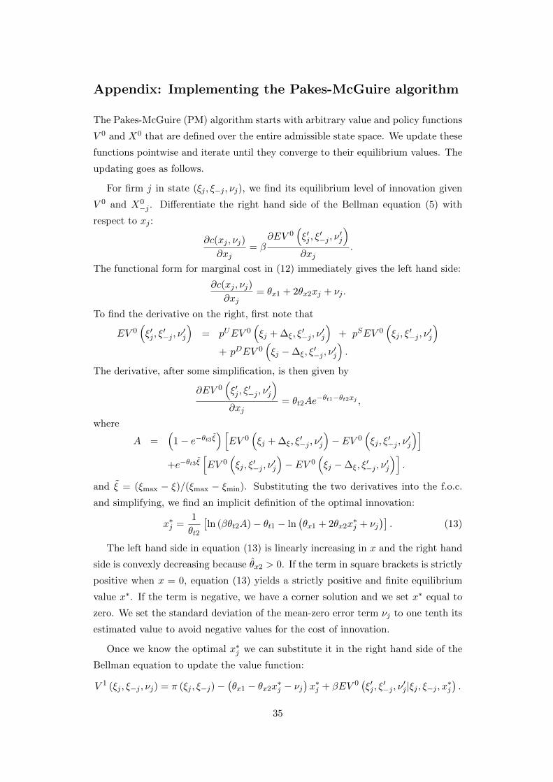
Appendix: Implementing the Pakes-McGuire algorithm
The Pakes-McGuire (PM) algorithm starts with arbitrary value and policy functions
V 0 and X0 that are defined over the entire admissible state space. We update these
functions pointwise and iterate until they converge to their equilibrium values. The
updating goes as follows.
For firm j in state (ξj , ξ−j , νj), we find its equilibrium level of innovation given
V 0 and X0−j . Differentiate the right hand side of the Bellman equation (5) with
respect to xj :
∂c(xj , νj)
∂xj= β
∂EV 0(ξ′j , ξ
′−j , ν
′j
)∂xj
.
The functional form for marginal cost in (12) immediately gives the left hand side:
∂c(xj , νj)
∂xj= θx1 + 2θx2xj + νj .
To find the derivative on the right, first note that
EV 0(ξ′j , ξ
′−j , ν
′j
)= pUEV 0
(ξj + ∆ξ, ξ
′−j , ν
′j
)+ pSEV 0
(ξj , ξ
′−j , ν
′j
)+ pDEV 0
(ξj −∆ξ, ξ
′−j , ν
′j
).
The derivative, after some simplification, is then given by
∂EV 0(ξ′j , ξ
′−j , ν
′j
)∂xj
= θt2Ae−θt1−θt2xj ,
where
A =(
1− e−θt3ξ̃) [EV 0
(ξj + ∆ξ, ξ
′−j , ν
′j
)− EV 0
(ξj , ξ
′−j , ν
′j
)]+e−θt3ξ̃
[EV 0
(ξj , ξ
′−j , ν
′j
)− EV 0
(ξj −∆ξ, ξ
′−j , ν
′j
)].
and ξ̃ = (ξmax − ξ)/(ξmax − ξmin). Substituting the two derivatives into the f.o.c.
and simplifying, we find an implicit definition of the optimal innovation:
x∗j =1
θt2
[ln (βθt2A)− θt1 − ln
(θx1 + 2θx2x
∗j + νj
)]. (13)
The left hand side in equation (13) is linearly increasing in x and the right hand
side is convexly decreasing because θ̂x2 > 0. If the term in square brackets is strictly
positive when x = 0, equation (13) yields a strictly positive and finite equilibrium
value x∗. If the term is negative, we have a corner solution and we set x∗ equal to
zero. We set the standard deviation of the mean-zero error term νj to one tenth its
estimated value to avoid negative values for the cost of innovation.
Once we know the optimal x∗j we can substitute it in the right hand side of the
Bellman equation to update the value function:
V 1 (ξj , ξ−j , νj) = π (ξj , ξ−j)−(θx1 − θx2x∗j − νj
)x∗j + βEV 0
(ξ′j , ξ
′−j , ν
′j |ξj , ξ−j , x∗j
).
35
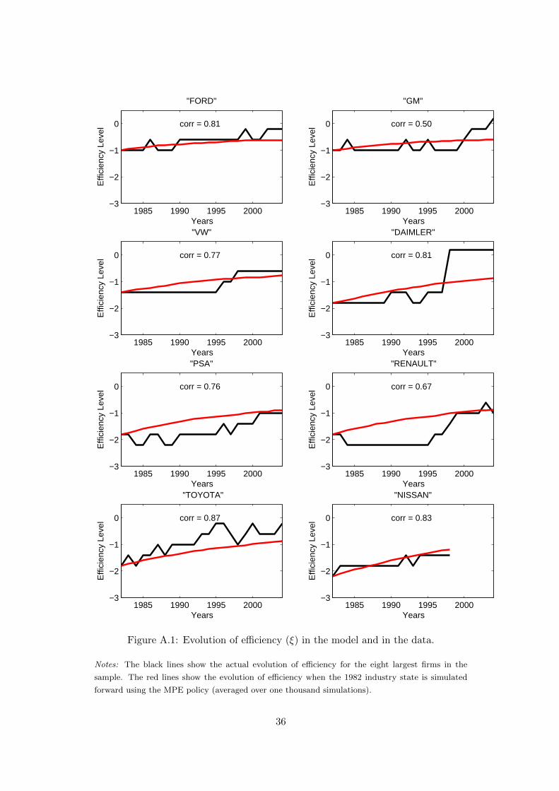
1985 1990 1995 2000−3
−2
−1
0 corr = 0.81
"FORD"
Years
Effi
cien
cy L
evel
1985 1990 1995 2000−3
−2
−1
0 corr = 0.50
"GM"
Years
Effi
cien
cy L
evel
1985 1990 1995 2000−3
−2
−1
0 corr = 0.77
"VW"
Years
Effi
cien
cy L
evel
1985 1990 1995 2000−3
−2
−1
0 corr = 0.81
"DAIMLER"
Years
Effi
cien
cy L
evel
1985 1990 1995 2000−3
−2
−1
0 corr = 0.76
"PSA"
Years
Effi
cien
cy L
evel
1985 1990 1995 2000−3
−2
−1
0 corr = 0.67
"RENAULT"
Years
Effi
cien
cy L
evel
1985 1990 1995 2000−3
−2
−1
0 corr = 0.87
"TOYOTA"
Years
Effi
cien
cy L
evel
1985 1990 1995 2000−3
−2
−1
0 corr = 0.83
"NISSAN"
Years
Effi
cien
cy L
evel
Figure A.1: Evolution of efficiency (ξ) in the model and in the data.
Notes: The black lines show the actual evolution of efficiency for the eight largest firms in the
sample. The red lines show the evolution of efficiency when the 1982 industry state is simulated
forward using the MPE policy (averaged over one thousand simulations).
36
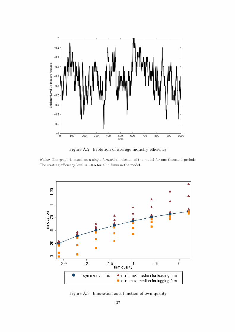
0 100 200 300 400 500 600 700 800 900 1000−1
−0.9
−0.8
−0.7
−0.6
−0.5
−0.4
−0.3
−0.2
−0.1
0
Time
Effi
cien
cy L
evel
(ξ),
Indu
stry
Ave
rage
Figure A.2: Evolution of average industry efficiency
Notes: The graph is based on a single forward simulation of the model for one thousand periods.
The starting efficiency level is −0.5 for all 8 firms in the model.
Figure A.3: Innovation as a function of own quality
37
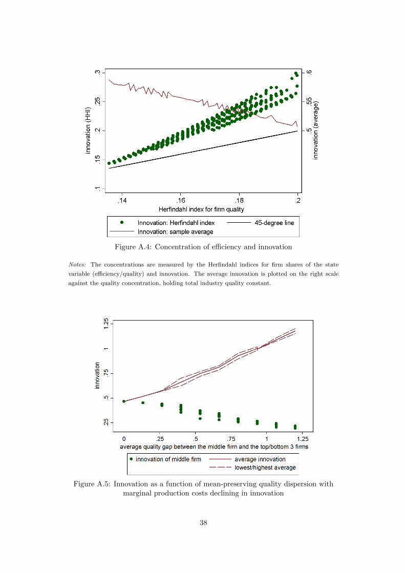
Figure A.4: Concentration of efficiency and innovation
Notes: The concentrations are measured by the Herfindahl indices for firm shares of the state
variable (efficiency/quality) and innovation. The average innovation is plotted on the right scale
against the quality concentration, holding total industry quality constant.
Figure A.5: Innovation as a function of mean-preserving quality dispersion withmarginal production costs declining in innovation
38