the relation between post-earnings announcement drift · it has been found that based on...
TRANSCRIPT

The Relation Between Post-Earnings Announcement Drift
and the Value Anomaly in the UK Stock Market
By
Pedro Jácome Henriques de Lancastre
Master Dissertation in Finance
Supervised by:
Professor: Júlio Fernando Seara Sequeira da Mota Lobão
2017

i
Biographical Note:
Pedro Lancastre was born and raised in Braga. Most of his life journey was made in his
home town, whereas he studied a Bachelor Degree in International Business and then a
Bachelor Degree in Management at University of Minho graduating in 2013.
During his lifetime he had some training courses abroad and he practiced sports mainly
football and tennis. He also does some volunteering work during his free time.
In 2014, he enrolled at FEP to start his master degree in finance, in which he developed
interest to follow career in this field.

ii
Abstract
Two of the oldest common anomalies that occur in the financial market are the value
anomaly and post-earnings announcement drift. Value anomaly consists in value stocks
that outperform growth stocks by having greater profitability with the same level of risk,
while post-earnings announcement drift consists in firms that report unexpected high
earnings outperform firms that report unexpected poor earnings by having greater
profitability with the same level of risk.
Both anomalies are provoked by different reactions in the market. The PEAD is provoked
by an underreaction and the value anomaly is caused by an overreaction as it concerns
when new information arrives, which have been part of study over the years among
experts. The aim of this study is to link both anomalies in the UK stock market, since
there is a lack of study in this field. Moreover, this study has theoretical relevance by
testing the efficiency market hypothesis to see if investors can beat the market and
practical relevance in the perspective of the investors to see if they can create a profitable
strategy taking advantage of the market anomalies.
It has been found that based on book-to-market, earnings-to-price, cash-flow-to-price and
sales growth classifications achieved a 29.84%, 36.6%, 45.52% and 25.72% annual
average abnormal return respectively.
This study in supporting with previous studies about anomalies in this market conclude
that UK stock market challenge the efficiency market hypothesis.
Key-words: Value anomaly, post-earnings announcement drift; market efficiency
hypothesis; overreaction, underreaction
JEL-Codes: G02, G14

iii
Sumário
Duas das mais comuns antigas anomalias que ocorrem no mercado financeiro são o valor
da anomalia e o post-earnings announcement drift. Valor da anomalia consiste em ações
de valor ultrapassarem em desempenho ao obter maiores rendibilidades do que as ações
de crescimento para o mesmo nível de risco, enquanto post-earnings announcement drift
consiste em empresas que apresentam inesperadamente maiores resultados obtêm melhor
desempenho ao conseguir maiores rendibilidades para o mesmo nível de risco do que
empresas que apresentam inesperadamente menores resultados.
Ambas anomalias são provocadas por diferentes reacções no mercado. O PEAD é
provocado pela sub-reacção e o valor da anomalia é o resultado de uma sobre-reacção no
que diz respeito à chegada de nova informação, o que tem sido parte de estudo ao longo
dos anos por especialistas. O objectivo deste estudo é ligar as duas anomalias no mercado
do Reino Unido, uma vez que há uma falha de estudo neste tema para este mercado. Além
do mais, este estudo tem relevância teórica ao testar a hipótese de eficiência de mercado
para ver se os investidores conseguem bater o mercado e tem também relevância prática
na perspetiva do investidor para saber se ele consegue criar estratégias lucráveis, tirando
vantagens das anomalias de mercado.
Foi encontrado com base nas classificações de book-to-market, earnings-to-price, cash-
flow-to-price e sales growth um retorno anormal médio anual de 29.84%, 36.6%, 45.52%
e 25.72% respectivamente.
Este estudo com base nos estudos anteriores sobre anomalias neste mercado conclui que
o mercado de ações do Reino Unido desafia a hipótese de eficiência de mercado.
Palavras-Chave: valor de anomalia, post-earnings announcement drift; hipótese de
eficiência de mercado, sobre-reacção e sub-reacção
JEL-Codes: G02, G14

iv
Index
1. Introduction ............................................................................................................................... 1
2. Literature Review ...................................................................................................................... 3
2.1 Post-Earnings Announcement Drift .................................................................................... 3
2.2 Value Anomaly ................................................................................................................... 5
2.3 Behavioral factors for Overreaction and Underreaction ..................................................... 8
2.3.1 Overconfidence and biased self-attribution .................................................................. 8
2.3.2 Representativeness heuristic......................................................................................... 9
2.3.3 Conservatism ................................................................................................................ 9
2.3.4 Bounded rationality .................................................................................................... 10
3. Methodology ........................................................................................................................... 11
3.1 Event Study ....................................................................................................................... 11
3.2 Models for Measuring Normal Performance ..................................................................... 14
3.2.1 Statistical models........................................................................................................ 14
3.3 Estimation of the Market Model ....................................................................................... 15
3.3.1 Abnormal Returns ...................................................................................................... 15
3.3.2 Cumulative Abnormal Returns ................................................................................... 17
3.4 Test Statistics .................................................................................................................... 18
3.4.1 Parametric Tests ......................................................................................................... 19
3.4.2 Non-Parametric Tests ................................................................................................. 20
3.5 The Value Anomaly Proxies ............................................................................................. 21
3.6 Market Expectations and Surprises ................................................................................... 22
4. Data and Descriptive Statistics ................................................................................................ 26
4.1 Data Selection ................................................................................................................... 26
4.2 Data Statistics .................................................................................................................... 28
5. Empirical Evidence ................................................................................................................. 33
5.1 Normality Test .................................................................................................................. 33
5.2 Sample Observations ......................................................................................................... 35

v
5.3 Results using Both Anomalies .......................................................................................... 38
5.3.1 Post-Earnings Announcement Drift using BM .......................................................... 39
5.3.2 Post-Earnings Announcement Drift using other proxies ............................................ 42
5.4 Regression Analysis .......................................................................................................... 43
5.5 Robustness Checks ............................................................................................................ 46
6. Conclusion ............................................................................................................................... 50
Bibliography ................................................................................................................................ 52
Appendix ..................................................................................................................................... 56
Appendix A: Extracted Variables ........................................................................................... 56
Appendix B: Formulas ............................................................................................................ 57
Appendix C: Portfolios using Both Anomalies ....................................................................... 60
Appendix D: Other Regressions and full Results .................................................................... 67
Appendix E: Robustness Check for other proxies................................................................... 85

vi
List of Tables
Table 1 - Frequency of the Subsample signs ............................................................................... 30
Table 2 - Summary Statistic ........................................................................................................ 31
Table 3 - Jarque-Bera Test for Normality ................................................................................... 34
Table 4a - Results: EAAR/ES portfolios using BM as a proxy ....................................................... 39
Table 4b - Results: EAAR portfolios using BM as a proxy ............................................................ 40
Table 5 - Regression Analysis for PEAD using BM ....................................................................... 44
Table 6a - Robustness Check: EAAR/ES portfolios using BM as a proxy – Size Effect ................. 47
Table 6b - Robustness Check: EAAR portfolios using BM as a proxy – Size Effect ...................... 48
Table 7 - Full Results: EAAR/ES portfolios using BM as a proxy .................................................. 60
Table 8a - Results: EAAR/ES portfolios using EP as a proxy ....................................................... 61
Table 8b - Results: EAAR portfolios using EP as a proxy ............................................................. 62
Table 9a - Results: EAAR/ES portfolios using CP as a proxy ........................................................ 63
Table 9b - Results: EAAR portfolios using CP as a proxy ............................................................. 64
Table 10a - EAAR/ES portfolios using SG as a proxy ................................................................... 65
Table 10b - Results: EAAR portfolios using SG as a proxy ........................................................... 66
Table 11 - Regression Analysis of PEAD using EP as a proxy ....................................................... 68
Table 12 - Regression Analysis of PEAD using CP as a proxy ....................................................... 69
Table 13 - Regression Analysis of PEAD using SG as a proxy....................................................... 70
Table 14a - Robustness Check: EAAR/ES portfolios using EP as a proxy – Size Effect ................ 85
Table 14b - Robustness Check: EAAR portfolios using EP as a proxy – Size Effect ..................... 85
Table 15a - Robustness Check: EAAR/ES portfolios using CP as a proxy – Size Effect ................ 86
Table 15b - Robustness Check: EAAR portfolios using CP as a proxy – Size Effect ..................... 86
Table 16a - Robustness Check: EAAR/ES portfolios using SG as a proxy – Size Effect ................ 87
Table 16b - Robustness Check: EAAR portfolios using SG as a proxy – Size Effect ..................... 88

vii
List of Figures
Figure 1 - Timeline for event study ............................................................................................. 13
Figure 2 - Sample Selection ......................................................................................................... 27
Figure 3 - Final Sample Selection for the Events ......................................................................... 28
Figure 4 - Number of Earnings Announcement per Quarter ...................................................... 29
Figure 5a - PEAD using proxies: EAAR/ES Portfolios - Value, Glamour and Hedge Portfolios .... 36
Figure 5b - PEAD using proxies: EAAR Portfolios - Value, Glamour and Hedge Portfolios ......... 37

1
1. Introduction
There are several anomalies that occur in the financial markets, which have been created
interest of study in the financial literature over the years and among them are the post-
earnings announcement drift and the value anomaly. Relevant literature found to cover
the existence of these anomalies (e.g. Foster et al. (1984), Bernard and Thomas (1989),
Lakonishok et al. (1994) and Liu et al. (2003)).
Recently, Yan and Zhao (2011) were the first and the only to link value anomaly directed
to the post-earnings announcement drift and analyse the relationship between the two
anomalies by covering the US stock market over 24 years, starting from 1984 until 2008.
Using calendar time portfolio formation and 1, 3, 6, 9, 12 months holding period and
BHAR as return metric, they found that a trading strategy taking a long position in value
stocks when both EARs and earnings surprise are positive and short position in glamour
stocks when both are negative can generate 16.6% to 18% annual returns.
To best of our knowledge since this theme is recent to link the two anomalies, there is a
lack of investigation in this field for other countries in which we intend to fill the gap in
the literature by linking the two anomalies as well fill emptiness of (in)efficiency research
on the UK stock market. We will rely on the Yan and Zhao (2011) study as our guideline,
since it is the only published study. This topic focuses on the relation between these two
anomalies and it has theoretical and practical relevance. It has theoretical relevance
because it has theoretical implication of the results by knowing if the markets are efficient,
and by that we want to know if stock prices would fully reflect all available and relevant
information at any given time. These anomalies question the validity of the efficiency of
the markets, therefore the idea of testing the efficient market hypothesis (EMH) is
important because it says that all stocks trade at their fair value because they reflect all
available information, so investors cannot beat the market. As for the practical relevance,
it is important for the perspective of the investor to see if they are able to create profitable
opportunities by taking advantage of the anomalies of the market by identifying
undervalued securities expecting that in the future will increase to outperform the market.
In this way, we intend to answer our research questions: Is there any relation between the
two anomalies? If the relation remains constant or not?

2
Our sample expands from 2010Q1 until 2015Q3 because we want to analyse the recent
years and the events that happened in the UK stock during this period of time to see if it
had any impact on the stock market and for the investor decisions.
Following the main author for this study, we intend to construct portfolios sorted into
quintiles based on the proxy classification with subsamples that vary with the direction
of the signs. The subsamples will be based on the earnings announcement abnormal
returns and earnings surprise performing a total of six sub-samples. Moreover, we add
two more subsamples based on the earnings abnormal return sign in order to have more
strengthens statistical tests and robustness for the EAAR/ES samples.
The results by linking the two anomalies for the UK stock market found some evidences
that challenge the Efficiency Market Hypothesis, as well significant drifts and the
presence of anomalies in the event-window and the post-event window. Moreover, we
found that our results for the 3-day event window and post-event windows are more
volatile for the value stocks than for the glamour stocks with the same level of risk
creating more profitable opportunities for the former than the latter stocks. In additionally,
the same applies for the robustness check when we study for the size effect, adding also
a small firm effect.
Besides this chapter, the study proceeds with the following chapters: chapter 2 literature
review, chapter 3 is the methodology, chapter 4 we describe the data and descriptive
statistics, chapter 5 portfolio results under the subsample signs condition for both
anomalies and we finish with chapter 6 where it remarks for conclusion, limitations,
further research and suggestions.

3
2. Literature Review
In this chapter contains evidence of literature review of both anomalies and possible
explanations. In this way, in section 2.1 we have post-earnings announcement drift,
section 2.2 value anomaly and section 2.3 behavior factors of underreaction and
overreaction.
2.1 Post-Earnings Announcement Drift
Post-Earnings Announcement Drift (PEAD) anomaly is an anomaly that occurs in the
financial market when firms report unexpectedly high earnings outperform firms
reporting poor earnings with the same level of risk. Ball and Brown (1968) were the first
to establish the existence of this anomaly through recognizing that following earnings
announcements, the estimated cumulative abnormal returns (CAR) continuously drifted
up in relation to firms announcing good news and continuously drifted down in relation
to firms announcing bad news (Bernard and Thomas, 1989).
The evidence of PEAD was later supported by studies such as Jones and Litzenberger
(1970) whereas in their investigation of quarterly earnings with a sample of stocks on the
US market from 1962-1967 found violations of the semi-strong efficiency by the fact of
the market not adjust instantaneously and correctly when new information arrives, instead
of that it reacts slowly and the results differ from the market.
Later, Foster et al. (1984) in their study on US stocks 1974-1981 observed a correlation
between abnormal returns and the unexpected earnings, by making a connection with size
of the firms. “The smaller the firm, the larger is the post-announcement cumulative
abnormal return with the positive (negative) earnings portfolios having positive
(negative) cumulative abnormal returns”. (p.598)
Moreover, Bernard and Thomas (1989) examine stocks in the US market over the period
1974-86 and found that a large amount of the drift that takes place in the first 60 days
following the announcement of earnings occurs within the first 5 days following the
announcement of earnings. They estimated for 240 days for post-announcement and
create an event-time portfolio formation with a size-adjusted risk control over the 120
days surrounding the earnings announcement date. In fact Bernard and Thomas (1989)
established that the percentage of the drift that occurs within the first 5 days following

4
the announcement of earnings in relation to the drift that takes place in the first 60 days
following the announcement of earnings is 13% for small firms, 18% for medium firms,
and 20% for large firms. In their empirical result to measure the magnitude of the drift,
they obtain a long position in the highest unexpected earnings decile and a short position
in the lowest decile would have yielded an estimated abnormal return of approximately
4.2% over the 60 days after the earnings announcement, or about 18% on an annualized
basis.
Bernard and Thomas (1989) explains that when the Earning based model is used it reflects
an identified risk premium which lead to PEAD been identified and this is because one
of the problems security model aims to alleviate is the risk adjustment problem of
Earnings based model.
Liu et al. (2003) show another study outside of US stock market. This study was made
for the UK stock market to find evidence of PEAD. They found evidence of PEAD,
confirm that this anomaly is not a specific market, but exists and persist in any stock
market. Extracting a sample period from 1988 until 1998, using a calendar time portfolio
formation and a 3, 6, 9, 12 months holding period with a three-factor model as risk
control, they use an alternative earnings surprise measures based on “(i) the time-series
of earnings; (ii) market prices; and (iii) analyst forecasts. Using each of the measures we
find evidence of significant post-earnings-announcement drift, robust to alternative
controls for risk and market microstructure effects (…) Our conclusion is that the UK
stock market is inefficient with respect to publicly available corporate earnings
information” (p.89).
Livnat and Mendenhall (2006) with a sample from US stocks from 1987-2003, holding
period of 4 quarters, using CAR as return metric, they obtained 5.21% PEAD return per
quarter. Concluding that differences comparing the analyst forecast to time series may
lead to mispricing.
Considering information uncertainty Francis et al. (2007) related with PEAD for the US
stock market between 1982-2001. With a calendar time portfolio formation and 6 months
holding period, using monthly alpha return metric and three/four factor model risk
control, they establish a connection whereas stocks where the investors have less

5
information and gain earnings with that create mutual initial reaction. Moreover, they
found that idiosyncratic volatility predicts the profitability of PEAD.
This phenomenon of PEAD can be explained by several hypotheses. Among them, the
most widely accepted explanation for this effect is that investors underreact to earnings
announcements, and this anomaly does not adjust as quickly as it should (Daniel et al.,
1998; Hong and Stein, 1999). Moreover, it is also widely believed that there is a strong
connection between earnings momentum and price momentum (Chordia and Shivakumar,
2006) .
Supporting the momentum evidence on the stock market Chan et al. (1996) found that it
is possible with earnings momentum strategy may benefit from underreaction to
information on short-term earnings, while a price momentum strategy may benefit from
the slow reaction of the market to response the arrival of the information, including the
long-term profitability.
In additionally, several studies such as Sadka (2006) also showed that the liquidity risk
could be one of the reasons of the earnings momentum as the Post-Earnings
Announcement Effect appears to be strong in small cap stocks.
Another two main reasons have also been part of discussion as a cause of PEAD supported
in the literature by authors such as Bernard and Thomas (1989) and Ball et al. (1988).
One of the causes is the delay price in response to new information, most explained that
traders do not use all available information or due to transaction and trading costs. The
other cause is the misspecification of CAPM, this cause is not plausibly and it is most
explained that this model to calculated abnormal returns is unfinished or wrongly
estimated.
Many theories have been suggested and stated for reasons of this phenomenon since the
first study of PEAD appointing for different arguments, but no consensus has been
reached among the experts.
2.2 Value Anomaly
The Value Anomaly is one of the oldest anomalies of the markets and it consists to be the
tendency of the value stocks outperforming growth stocks with the same level of risk.
Graham and Dodd (1934) were the first to establish the concept of value anomaly by

6
recognizing the importance of paying a low price for stocks and make a definition of these
two types of stocks (value and growth) in their study.
The importance of paying low price for stocks came because value stocks systematically
outperform growth stocks with the same level of risk. Although, smaller stocks are more
difficult to value because they are riskier; have less information; more difficult to profit
from that and have higher transaction costs, investors when are optimistic are willing to
pay a lot for smaller stocks. Indeed, in times of recession investors are willing to pay more
for value stocks because they have a better performance than growth stocks, while growth
stocks are stronger in periods of expansion (Chan and Lakonishok, 2004).
If firms do not have a long historic about smaller stocks, it will affect the mood of the
investors. The main explanations have to do with the sentiment. These stocks are also
difficult to arbitrage because it is difficult to profit from that, once it has no derivatives.
Value stocks are low profile securities that are traded at a lower price relative to its
fundamentals. This kind of stocks are characterized to have low (price-to-earnings; price-
to-book; price-to-cash flow; dividends) and others measures of their fundamentals in
relation to the market average (Fama and French, 1992; Fama and French, 1996). These
stocks are considered to be part of investors that use contrarian strategies, once according
to Fama and French (1992) they are fundamentally riskier. So, investors consider them to
be underpriced and because of that they can produce superior returns in compensation for
the risk.
The successful of this investment strategy is because they are contrarian to “naïve”
strategies. These naïve strategies results from the lack of sense of the investor in reading
the price market signs making an overreact or underreact in the process of the information.
While, the contrarian investors bet against naïve investors because they invest in
underpriced stocks and not in overpriced stocks by that outperforming the market (De
Bondt and Thaler, 1985; Conrad, 1995).
Additionally, the value strategy with the value investment philosophy supported by
Graham and Dodd (1934) as stated before contrary the efficient market hypothesis that
says that the market incorporates all relevant information, making it impossible to profit
from undervalued stocks.

7
On the other hand, glamour stocks are shares in a company whose their earnings and sales
are growing faster than those in other companies and are expected to continue to growth.
According to Bourguignon and de Jong (2003) this type of investment style requires to
investors a longer time-horizon by looking companies in booming industries for the
expectation of rapid growing earnings and sales. In this sense, this contradicts the value
stocks whereas the investor uses their strategy in short-horizon expecting to achieve gains
from price momentum.
From Lakonishok et al. (1994) study they found that one of the reasons why value stocks
outperform growth stock is because investors overestimated future growth rates of
glamour stocks relative to value stocks. They use sample of US stocks from the period
1968-1990, with a calendar time portfolio formation and with 12 months holding period,
they used B/M; E/P; C/P and GS ratios as proxies to capture value anomaly. The results
present a 10%-11% value anomaly per year with a long positive position and a short
negative position.
In their study, they documented “value strategies” linking their higher returns to
“overreaction hypothesis”. This happens because although, the evidence of mean
reversion on growth forecast these strategies are contrarian investors and are able to
exploit the naïve investors behavior or because they are riskier.
A challenge to the EMH is the individual’s reaction to news. The most valuable
commodity that we can have is information and with that people tend to overreact or
underreact. However, some investors could in turn take advantage of people’s reaction
which create a market anomaly and use their expertise to take advantage by profiting with
that. On the other hand, the overreaction and underreaction could be consistent with the
efficiency market hypothesis if both split randomly (Fama 1998).
Investors overweight to new information because that newly information is salient and
captures their attention, so it becomes important for them and have a heavy weight in
terms of making decision resulting in overreaction whereas prices are pushed beyond the
levels warranted by fundamentals.
On the other hand, investors that underweight the arrival of new information cause
underreaction. In this sense, it is possible to affirm that there is a lack of incorporation of

8
new information into stock prices such as earnings announcement and this underreaction
continue until prices fully incorporate all information available.
Despite the evidence of overreaction and underreaction Fama (1998) says that both are
equally common. This is not supported with the previous studies when both phenomena
act in different time horizons.
However, this view is not consistent with Lee and Swaminathan (2000) showing that past
trading volume provides an important link between “momentum” and “value” strategies,
whereas these findings support the intermediate-horizon “underreaction” and the long-
horizon “overreaction” effects.
The value anomaly is considered to be inconsistent with the CAPM model, once the value
stocks tend to have higher expected returns than CAPM, while the growth stocks tend to
have lower expected returns in comparison to the CAPM prediction.
2.3 Behavioral factors for Overreaction and Underreaction
The behavior of investors is related as an explanation of both reactions, as this factor is
attributed as the cause of investors having overconfidence and biased self-attribution;
representative heuristic; and to have bounded rationality concerning their overreaction to
new information, while they are considered to have conservatism and bounded rationality
concerning their underreaction to new information.
2.3.1 Overconfidence and biased self-attribution
Daniel et al. (1998) made a theory connecting the overconfidence to self-attribution bias,
saying that this comes from the ability of the investors to think that they are smarter than
the average and that they rarely make mistakes with their assumptions.
According to the authors, the investors weights their private information comparing to
public signals. Depending on the confirmation or not of the signals is what makes them
to overreact or underreact. Normally, their overconfidence makes them overreact due
private information, they trade with the information that they have even is irrelevant to
gain with that and only adjust slowly when public signals contradict it.
So, people are overconfident and that explains the excess volatility of asset prices because
people overweight the information that they own.

9
The overconfidence and self-attribution also cause the continuing overreaction implying
momentum in prices in the short-term, but the momentum is reversed when public
information correct prices back to their fundamentals. So, stock prices are more volatile
than fundamentals. Thus, these factors are also mean reversion in the long-term.
2.3.2 Representativeness heuristic
The representativeness heuristic was first theorized by Tversky and Kahneman (1974).
This theory is used by people that take judgments and make decisions about the
probabilities of an event under uncertainty. The authors of this theory argue that people
rely on limited heuristic principles, reducing complex tasks of assessing likelihoods and
predicting values to simple judgmental operation but sometimes they lead to severe and
systematic errors. Nevertheless, the authors affirm that heuristics are useful because
reduce our effort and time by simplifying our decision.
In contradiction, Gigerenzer (1996) disagree with the theory developed by Tversky and
Kahneman (1974). He argues that this method explains everything and nothing at the
same time, adding that the judgments and decisions should not take always be based in
statistics and probabilities and it could be based made by asking questions of frequencies.
Later, Barberis et al. (1998) present a model of investor sentiment stating with the
representativeness people think they see actual earnings follow a random walk and the
investors do not understand this, creating an overreaction because if they see growing
earnings of a firm and due the random path of the earnings they might not continue to
growth. Thus, it is created disappointment once they overweight and underweight the
information and as consequence get contradictions results.
2.3.3 Conservatism
Basu (1997) find evidence of conservatism in result of earnings reflecting more quickly
“bad news” than “good news”.
Following that path, Barberis et al. (1998) based on the model previously stated, the
investors are very stuck with their prior beliefs and for that they are slow to make
adjustments of the underweight information and that contributes for the underreaction to
new information.

10
These implications may lead to investors makes mistakes and assume that the firm is
mean-reverting.
2.3.4 Bounded rationality
Bounded rationality is one of main behavior explanation of the investors and takes as
consequence the creation of the overreaction and underreaction.
Hong and Stein (1999) defined two groups of boundedly rational agents: “news watchers”
and “momentum traders”. The “news watchers” do not pay attention to prices, only to
news and the “momentum traders” only look at past prices. So, both are risk averse
because do not evaluate a part of the information available.
The news watchers adjust prices slowly only to new information, so there is only
underreaction resulting in a combination of gradual information diffusion with the
assumptions.
On the other hand, momentum traders want to profit from the underreaction caused by
news watchers and they use simple strategies by looking only to past prices, so they are
pushing the price of winners above their intrinsic value creating overreaction to any news.
Their model generates underreaction and price momentum in the short-term and
overreaction and mean reversion in the long-term.

11
3. Methodology
In this chapter, it is described the methodology used for study. The first subsection
presents the overall framework for this study, second and third subsections present the
choice of models and formulas to apply for the study and test statistics, the fourth
subsection explain the tests statistics and finally the fifth and the sixth section explain the
proxies and subsamples used for this study.
3.1 Event Study
From the literature review chapter, it was possible to conclude that post-earnings
announcement drift and value anomaly violates the semi-strong form efficiency market
hypothesis. So, in this sense it is important to introduce an event study approach to test
the performance of the capital markets. The underlying assumption of this approach is
that capital markets is semi-strong form efficiency. For that, it is necessary to measure
the valuations effects of the earnings announcements as well as examine the response of
the stock price around the earnings announcement of the event by treating and process
the data in MS Excel and ESM software.
The event study framework has not changed drastically since the late 1960’s when Ball
and Brown (1968) and mainly when Fama et al. (1969) introduced their methodology
concerning the estimation of abnormal returns (AR) as important measure to test the
market’s efficiency in response to stock split announcements. Moreover, Fama (1991)
states that event studies are an important part of finance and says that:
“Event studies are the cleanest evidence we have on efficiency” (Fama, 1991, p. 1602).
An event study more specifically, show the analysis and evidence of the impact of news
and events related directly or indirectly to the company, its stocks as well as the industry,
sector or overall market and any capture of the abnormal returns may result a detection
of markets’ inefficiency. If markets are informationally efficient, then the event should
reflect immediately on the announcement date and not on the following trading days. That
is why event studies are often considered to test the efficiency of the market.
There are short (< 1 year) and long-horizon (> 1 year up to 5 years) event studies. The
short-horizon event studies are more reliable than the long-horizon event studies.
Although the long-horizon event studies have been improved in last years, Kothari and

12
Warner (1997) say that these event studies still involve many issues and there is still a
path to improve.
In order to construct an event study, it is necessary to design an event study timeline. In
this sense, following the standard event study technique by Brown and Warner (1985)
there are three important periods to define. Firstly, the estimation window, also as known
as the control period, whereas estimate the market model which is used to determine the
normal behavior of a stock’s return in comparison with the market or industry index and
it is normally used the regression model to determine this “normal” behavior. Secondly,
the event window whereas it often starts a few trading days before the actual event day
happen and length it is usually centered on the announcement. Based on actual returns
during the event window and the “normal returns” predicted, “abnormal returns” are
calculated for all days with the event window. This period of the timeline along with the
abnormal returns are important to examine if whether the event announcement was
anticipated, leaked or if the “post-announcement effect” needed more time to absorb the
information content of the event and another reason is if the material of the event was
relevant for the content in cause.
Finally, we have the post-event window which is considered when a company makes an
announcement or when an event significant occurs that makes impact on the market and
this also allow us to measure the long-term impact of the event. Normally, the post-event
window is associated to investigate the performance of the company following
announcements when a major acquisition or an IPO happens.
For this event study the firms of the market extracted from the United Kingdom will be
used the quarterly earnings announcement. Additionally, this study focuses on 23 quarters
from 2010Q1 to 2015Q3 and for the firms that announce earnings during the trading day,
the event date will be the date of the announce and if the firms announce after the closing
bell the event date will on the following day. Moreover, Jones and Litzenberger (1970),
Foster et al. (1984), Bernard and Thomas (1989) and Yan and Zhao (2011) confirm the
importance of collecting quarterly data as well the earnings surprise factor to exploit the
post-announcement security return results. Since, the aim is to investigate the post-event
window where possible post-announcement drift can occur and as we know the drift is
commonly seen within 3-months after the earnings announcement.

13
The estimation window should be chosen in a way that the returns are not compromised
with their performance with the event. Armitage (1995) suggest that the estimate period
should range from 100 to 300 days. But, MacKinlay (1997) says that for the most common
model, the market model, for the measure of normal returns it should be implemented an
estimation window with a size of 120 days. We decided to follow Mackinlay (1997) and
use the 120 days, since it also belongs to the period range purposed by Armitage (1995).
As it concerns to the event window will be similar to Yan and Zhao (2011), it will be
looked the drift starting from the second day after the current quarter´s earnings
announcement and ends on the second day prior to the next quarter´s earnings
announcement. The same approach of the author will happen for the post-event window
in examine drift patterns in each sub-sample in the subsequent periods, starting from the
second day after the earnings announcement up to 1 month (22 trading days), 3 months
(63 trading days), 6 months (126 trading days), 9 months (189 trading days) and 1 year
(252 trading days) after the earnings announcement.
Thus, in this sense this should be long enough to calculate meaningful estimates of normal
returns. Otherwise, a shorter sub-sample could affect the construction of expected returns.
So, the choice of this event study as short-term is perfect to exclude any confounding
effects and the sub-samples are long enough to capture any significant effect of the event.
The timeline for event study is illustrated in figure 1
Figure 1 - Timeline for event study
Estimation Window Event Window Post-Event Window
T0 T1 T2 T3
-120 -1 0 1 22 63 126 189 252
Source: Own Creation
Time

14
3.2 Models for Measuring Normal Performance
The event studies are used to measure the impact of a specific event on the value of firms
or prices. That is why it is necessary to choose the appropriate normal return model.
MacKinlay (1997) describe that there are two categories of models to be followed in order
to estimate normal returns: statistical and economic. In additionally, he says that the
former category follows from statistical assumptions concerning the behavior of asset
returns and do not depend on economic arguments. On the other hand, the latter category
relies on assumptions concerning on investors’ behavior and are not based only on
statistical assumptions. However, it is needed to add statistical assumptions to put the
economic model in practice. We followed the statistical model.
3.2.1 Statistical models
The right and the most popular model according to the financial literature for an event
study determine that this thesis will rely on the Market Model in the calculation of the
expected normal returns.
The Market Model is probably the most common approach to construct expected returns.
It is a more slightly sophisticated approach in which the return on a security depends on
the return on the market portfolio of security’s receptiveness as measured by beta. In this
sense, this model will overcome the impact of general market movements in a
rudimentary way, once this model assumes a constant and linear relation between
individual asset returns and the return of a market index. The use of this model compared
with the former model reduces variance of abnormal return, which implies more powerful
tests (CLM, 1997).
Ri,t = αi + βi (Rmt) + ei,t
With
E[ei,t] = 0 and VAR[ei,t] = 𝜎2εi (3.2.1.1)
Ri,t is the return on asset i on period t, Rmt is the return on portfolio m on period t, αi is
the intercept of the value of Ri when Rm equals to zero, βi is the slope (estimate of the
systematic risk for asset i), ei,t is the zero mean error term on the security i on the period
t. Moreover, the variance (𝜎2εi), beta (βi), alpha (αi) and the error term (ei,t) are the

15
parameters of the model, estimated by the Ordinary Least Squares (OLS) method. These
parameters are estimated in the estimation period for each observation. The formulas for
the estimation of the parameters can be seen in equation 3.2.1.1, Appendix B.
In the Brown and Warner (1980) paper, they observed stock return data into various
methodologies in event studies to measure security price performance based by the
examination of the frequency of type I and type II errors and calculating the power of
each methodology. Their findings prove that a simple methodology based on the market
model performs well under a wide variety of conditions and the use of more sophisticated
models can result in false inferences about the presence of abnormal performance.
Based on these evidences, the right and the most popular model in the financial literature
determine that this thesis will rely on the Market Model in the calculation of the expected
normal returns.
3.3 Estimation of the Market Model
Through the choice of the market model with the appropriate estimate procedure (OLS)
for the parameters made in the previous sub-section, the respectively choice of methods
and calculations for this model will be deeply explained in the following sub-sections
considering the choice of the UK stock market (London Stock Exchange).
3.3.1 Abnormal Returns
The abnormal returns are the difference between the actual return and expected return
from the market movements, making them as essential measure to evaluate the impact of
an event. In this way, these measures are important to help in auditing for a conclusion if
a portfolio manager’s skills on a risk-adjusted basis and if the investors were appropriately
compensated for the risk that they assume. The abnormal returns can be calculated by the
following formula:
𝐴𝑅𝑖, 𝑡 = 𝑅𝑖, 𝑡 - �̂� - �̂�𝑖𝑅𝑚𝑡 (3.3.1.1)
Where, 𝐴𝑅𝑖, 𝑡 is the abnormal return, which is the disturbance term 𝜀𝑖𝑡 in the event
window of the market model for firm i at the period t, 𝑅𝑖, 𝑡 is the actual return for firm i
at the period t and the �̂� - �̂�𝑖𝑅𝑚𝑡 is the expected return for firm i at the period t.

16
The daily stock returns are used with the logarithmic function to make the return
distribution, converge to normality and to eliminate negative returns according to the
market model and the tests used. This is consistent with the findings of Corrado and
Truong (2008) were they found that the logarithmic returns perform better test
specification in event studies. The daily logarithmic return for both stock and market are
calculated in the following formula:
𝑅𝑖, 𝑡 = LN (𝑆𝑡𝑜𝑐𝑘 𝑝𝑟𝑖𝑐𝑒 𝑡
𝑆𝑡𝑜𝑐𝑘 𝑝𝑟𝑖𝑐𝑒 𝑡−1) ; 𝑅𝑚𝑡= LN (
𝑀𝑎𝑟𝑘𝑒𝑡 𝑖𝑛𝑑𝑒𝑥 𝑝𝑟𝑖𝑐𝑒 𝑡
𝑀𝑎𝑟𝑘𝑒𝑡 𝑖𝑛𝑑𝑒𝑥 𝑝𝑟𝑖𝑐𝑒 𝑡−1) (3.3.1.2)
Where, 𝑅𝑖, 𝑡 is the logarithmic return of the stock i for the period t divided by the
logarithmic return of the stock i for the day before the period t. The same applies for the
market formula, 𝑅𝑚𝑡.
There are two different measures to aggregate abnormal returns that normally used in the
finance literature for an event study: BHAR (Buy-and-Hold Abnormal Returns) and CAR
(Cumulative Abnormal Returns).
The BHAR model is based on the principle of the long-term where it gives the best
returns. This kind of model is calculated by the difference between the realized buy-and-
hold return and the normal buy-and-hold return and it is often used for long-term event
studies such as IPO or when a major acquisition happens (Loughran and Ritter, 1995;
Fama, 1998). Furthermore, Barber and Lyon (1997) and Lyon et al. (1999) advocate this
model and say that the BHAR model better match the investor investment experience and
eliminates the problem of cross-sectional dependence among the sample firms.
However, this method requires a benchmark sample or matching stock that have not
experience the event. Since, as it was said before every firm of the sample report their
earnings quarterly, semi-annual or even annually and because of that the latter
requirement is impossible to do. Besides that, we want to study earnings announcement,
so every firm will experience the event at some day. Moreover, the MSCI UK was chosen
as index for this study instead of the benchmark because we believe it measures with
more precise all the constituents of the LSE stock market and it seems more appropriate
for this kind of study.
While it is true that BHAR perform better for long-term studies, it is also true that the
CARs perform better for short-term studies. Furthermore, Fama (1998) argues in favor of

17
the use of CARs instead of the BHARs given the theoretical and statistical considerations.
For these reasons, we decided to use the Cumulative Abnormal Returns method.
3.3.2 Cumulative Abnormal Returns
A hierarchy of abnormal returns calculated are compounded to cumulative abnormal
returns (CARs), which can be averaged to cumulative average abnormal returns (CAARs)
in cross-sectional studies.
The cumulative abnormal return method is normally used to determine how accurate the
model is. More often, it is used to investigate the impact of any affect extraneous events
on the stock prices. In additionally, Kothari and Warner (2008) say that for testing the
semi-strong form of EMH, this measure should be used in order to see how fast the market
react to new information.
The CARs method is the sum of the abnormal returns of the stock i at the period t and it
is represented as:
𝐶𝐴𝑅𝑖(𝑇1, 𝑇2) = ∑ 𝐴𝑅𝑇2𝑡=𝑇1 𝑖, 𝑡 (3.3.2.1)
Where, the cumulative abnormal returns over a multi-period event window by summing
the average returns from the period T1 until the period T2. This can also be applied to the
post-event window starting from the period T2 and goes until the period T3.
Following, the analysis performance of abnormal returns for multiple events it may give
typical stock market response patterns. So, the typical abnormal returns associated with a
specific period of time of N events before and after the event day give us the following
formula for average abnormal returns:
𝐴𝐴𝑅 = 1
𝑁 ∑ 𝐴𝑅𝑖,𝑡
𝑁
𝑖=1 (3.3.2.2)
After following the abnormal, cumulative and average returns formulas we are able to
form the cumulative average abnormal returns (CAARs) where it has great statistical
analysis importance in addition with the AAR because it assembles the effect of the
abnormal returns. The CAAR based on cross-average measure for both event-window
and post-window is defined by the following formula:
𝐶𝐴𝐴𝑅 (𝑇1, 𝑇2) = 1
𝑁 ∑ 𝐶𝐴𝑅𝑖(𝑇1, 𝑇2)𝑁
𝑖=1 (3.3.2.3)

18
The statistical tests considering these measures will be approached deeply in the
following section.
3.4 Test Statistics
The power of using test statistics is very accurately in precisely the capture of any
abnormal returns that differ from zero with some statistical validity. The literature on
event study test statistics is very rich, as well the significance tests. CLM (1997) claim
that:
“The significance of using statistical test on an event study is the ability to detect the
presence of false null hypothesis. Thus, the likelihood that an event study test rejects the
null hypothesis for a given level of abnormal return associated with an event is the power
of the test” (CLM., 1997, p.168).
The CAARs use the T-Tests to test the efficiency of the markets, this is the hypothesis of
the CAARs being or not equal to zero defined as:
Ho: CAAR = 0 H1: CAAR ≠ 0
Hence, the rejection of H0 confirms a presence of anomalies in the market. A rejection of
H1 confirms otherwise.
This study, will include three different statistical tests in order to achieve the main purpose
of the investigation. One parametric tests (Standardized Residual Test) and two non-
parametric tests (Rank Test and Generalized Sign Test).
Parametric tests assume that the individual firm’s abnormal returns are normally
distrusted. So, it makes more assumptions and the parametric data underlies on normal
distribution, which allows to make more conclusions. Campbell and Wasley (1993) say
that the normality of abnormal returns is a key assumption underlying to use the
parametric tests for event studies. The non-parametric tests are based on a fewer
assumptions and for that are less powerful than the parametric tests. However, Corrado
(1989) on his paper describe statistic superiority of non-parametric tests over parametric
tests in the returns case has been documented even departures from normality are not
pronounced.

19
The following sub-sections will describe deeply each of both parametric and non-
parametric tests to be used.
3.4.1 Parametric Tests
The parametric test used for this event study was the standardized residual test because is the
most popular parametric statistical test, once it has been found more robust considering
possible volatility changes associated with the event. For details about this parametric test
could be found in the following description.
T1: Standardized Residual Test
The Standardized Residual Test also as known as the Patell Test is a complement of the
cross-sectional independence test. It was developed by Patell (1976) and the
standardization reduces the effect of the stocks with large returns, it assumes cross-
sectional independence in abnormal returns and assumes that there is no event induced
change in the variance across of the event period of abnormal returns. It is estimated as:
𝑆𝐴𝑅𝑖, 𝑡 = 𝐴𝑅 i,t
𝑆(𝐴𝑅 i,t) (3.4.1.1)
Where the standard deviation is according to his facts that the event-window abnormal
returns are an out-of-sample forecast and the standard error is adjusted by the forecast
error:
𝑆𝐴𝑅𝑖,𝑡2 = 𝑆𝐴𝑅𝑡
2 (1 + 1
𝑀𝑖+
(𝑅𝑚,𝑡− �̅�𝑚)2
∑ (𝑅𝑚,𝑡− �̅�𝑚)2𝑇1𝑡=0
)
After calculating SAR, we have:
𝑆𝐶𝐴𝑅𝑖 = ∑ 𝑆𝐴𝑅𝑖, 𝑡𝑇2𝑡=𝑇𝑖,𝑇2
And finally, to get the patell test:
𝑇1 𝐶𝐴𝐴𝑅 = 1
√𝑁 ∑
𝑆𝐶𝐴𝑅𝑖
𝑆𝑆𝐶𝐴𝑅𝑡
𝑁𝑖=1
With,
𝑆𝐶𝑆𝐴𝑅𝑡2 = 𝐿2
𝑀𝑖−2
𝑀𝑖−4

20
Boehmer et al. (1991) found that under the absence of an event induced variance increase,
and that this test is well specified and has appropriate power.
3.4.2 Non-Parametric Tests
The following non-parametric test for this event study are the rank teste and the generalized
sign test, which could be found in the following description.
T2: Rank Test
The Corrado (1989) Rank Test consider a combination of both post and event window as
well the estimation period into a single set of returns and ranked them based on return to
each daily for each firm: 𝐾𝑖,𝑇 = 𝑟𝑎𝑛𝑘 (𝐴𝑅𝑖𝑇), where t = -120, …, 252. This test ranks
from the lowest abnormal return until the highest abnormal return. To get the rank test,
we need to follow the following steps:
�̅�𝑇1,𝑇2 = 1
𝐿2 ∑ �̅�𝑡
𝑇2𝑡=𝑇1+1 , where �̅�𝑡 =
1
𝑁𝑡∑ 𝐾𝑖𝑡𝑁𝑡
𝑖=1 (3.4.2.1)
Where, statics test is:
𝑇2 𝐶𝐴𝐴𝑅 = √𝐿2 (�̅�𝑇1,𝑇2 − 0.5
𝑆�̅�
)
And for standard deviation, we have:
𝑆�̅�2
1
𝐿1+𝐿2 ∑
𝑁𝑡
𝑁
𝑇2𝑡=𝑇𝑖 (�̅�𝑡 − 0.5)
T3: Generalized Sign Test
The Generalized Sign Test is an improvement of the Sign Test and was adopted by Cowan
(1992), where it compares the proportion of positive AR around an event to a proportion
that was not affected by the event. So, it allows the null hypothesis having positive AR to
be different from 0.5. Moreover, this test is a binomial test whether this positive AR
equals to 50% or not.
The generalized sign test provides more powerful than a parametric test based on standard
errors from cross-section of event date abnormal returns and becomes more powerful as
the length of the event window increases (Cowan, 1992).
It is calculated with the following formulas:

21
�̂� = 1
𝑁 ∑
1
𝐿1
𝑁𝑖=1 ∑ 𝜑𝑖𝑡
𝑇𝑖𝑡=𝑇𝑖 where, 𝜑𝑖𝑡 = 1 if the sign is positive, and 0 otherwise. (3.4.2.2)
And the GST is:
𝑇3 𝐶𝐴𝐴𝑅 = (𝑤−𝑁�̂�)
√𝑁�̂�(1−𝑝)
Where, w is the number of stocks in the event window for which CAR is positive.
3.5 The Value Anomaly Proxies
Following the Lakonishok et al. (1994) and the Yan and Zhao (2011) studies, we will use
the four empirical proxies to capture the value anomaly effect: book-to-market (BM),
earnings-to-price (EP), cash-flow-to-price (CP) and sales growth (SG). As we already
know, the value stocks are characterized for having high (book-to-market; price-to-
earnings; cash-flow-to-price) and low sales growth, while in the opposite way is classified
for the growth stocks.
The use of these multiples to make classification on the value anomaly is recognized by
several scholars (see e.g., Fama and French (1993); Lakonishok et al. (1994) Barberis and
Shleifer (2003); Bourguignon and de Jong (2003)).
In additionally, Fama (1998) says that these multiples produce stable results in returns.
However, the dividend-to-price (D/P) is also used by these authors, but the problem of
this proxy is that produce a weaker performance compared with the other multiples.
The book-to-market compares the book value of a firm to its market value. According to
Fama and French (1992) this measure has a strong role in explaining cross-sectional
average returns on the stocks of the stock exchange. Moreover, Fama and French (1995)
say that the market and size factors can explain the behavior of earnings, but there is no
link between the B/M factors in earnings and returns.
Regarding the earnings-to-price compares the P/E of a stock to a cumulative P/E of a
related market index. This is useful because it helps if the performance of a stock was
adequate or not to the overall market performance. Basu (1983) shows that E/P also help
to explain the cross section of average returns, and Ball (1978) argues that E/P is a catch-
all proxy for unnamed factors in expected returns (Fama and French, 1992).

22
The cash-flow-to-price compares the amount of cash-flow generated to the price of a
company. It offers to investors a useful tool to look to the company’s value more than
P/E because it not includes the depreciation effects as well as the accounting differences
related with depreciations. According to Bodie et al. (2009) this ratio is important as
multiple because it defines the expectation of a stock’s firms price to reach when
generates a certain level of cash flow.
Finally, we have the sales growth in which following Lakonishok et al. (1994) it consists
as the average of annual growth in sales over the previous five years. It is useful because
it determines trends and how investors are prone to regard a stock with low cash flow
relative to price and high past sales growth as having more promising future growth
prospects (Chan and Lakonishok, 2004).
The positive and negative of the multiples could be considered by scholars as a neglect.
Fama and French (2007) argue that both signs are largely unexpected, while Huang et al.
(2012) say that negative multiples causes noise to the sample. Nevertheless, we will be
consistent with Lakonishok et al. (1994), Desai et al. (2004) and Yan and Zhao (2011)
studies and not remove the EP and CP ratios because the negative of these multiples has
increased in recent years and if we cut it will imply a huge cut for the final sample (Collins
et al. 1999). However, we will eliminate the negative book-to-market ratios.
3.6 Market Expectations and Surprises
In order to form portfolios and detect market reaction to the event, we will follow LaPorta
et al. (1997) and Yan and Zhao (2011) approach and use the Earnings Announcement
Abnormal Return (EAAR).
The market expectations have influence on how the investor or investment managers
allocate their assets in a portfolio considering the expected risks and returns, whereas
these assumptions increase when the assets allocated are exposed to favorable scenarios,
and decrease when assets allocated are exposed to unfavorable scenarios. So, when the
market expectations are taking into account it is seen as a crucial undertaking.
In this way, the time sensitivity is a crucial factor that can shift the market expectations
due to the tendency for data to modify in response to a large range of factors. Therefore,
based on the number of observations and the group of EAARs to form portfolios, the

23
market expectations signs will result on the outcome of the capture sign of the EAARs.
This is, when there is a negative sign of the market expectation, the same sign will have
the EAARs as so when there is a positive sign of the market expectation, the same sign
will have the EAARs:
• Negative Market Reaction (-): EAAR < 0
• Positive Market Reaction (+): EAAR > 0
As concerning the importance of the market expectations Fried and Givoly (1982) in their
study measure the performance of an alternative surrogate for the same and knowing from
a previous study that they made in which analysts’ forecasts have information content,
their results indicate prediction errors are more associated with the price security
movement and with that they were able to conclude that:
“Analysts’ forecasts provide a better surrogate for market expectations than forecasts
generated by time-series models” (Fired and Givoly, 1982, p.85)
The main reason, according to the authors why time series models as an alternative for
the market expectations are not so reliable is because is further impaired by the underlying
assumptions that the earnings generating process are stationary along with stable
parameters and the characteristics of the model is applied to all firms involved.
In the literature, there is a distinguish views to apply EPS surprises method, some use for
time series models while others use for analysts’ forecasts.
Skinner and Sloan (2002) show that growth stocks exhibit an asymmetric response to
earnings surprises. Demonstrating, that while growth stocks are at least as likely to
announce negative earnings surprises as positive earnings surprises, they exhibit an
asymmetrically large negative price response to negative earnings surprises.
While, Brandt et al. (2008) state that earnings surprises represented by SUE do not
represent all the stock abnormal returns around the earnings announcement date. Adding
to that, the 14%-15% of the firms subject it to SUE approach experience extreme
announcement returns in exactly the opposite direction of the earnings surprise.
We will rely and follow the method provided by Yan and Zhao (2011) based on the
analyst forecasts.

24
The formula that they used can be translated as the difference between the reported EPS
and the expected EPS, divided by the absolute value of the expected EPS1:
𝐸𝑎𝑟𝑛𝑖𝑛𝑔𝑠 𝑆𝑢𝑟𝑝𝑟𝑖𝑠𝑒𝑖𝑞 = 𝑅𝑒𝑝𝑜𝑟𝑡𝑒𝑑 𝐸𝑃𝑆𝑖𝑞−𝐸𝑥𝑝𝑒𝑐𝑡𝑒𝑑 𝐸𝑃𝑆𝑖𝑞
𝑎𝑏𝑠(𝐸𝑥𝑝𝑒𝑐𝑡𝑒𝑑 𝐸𝑃𝑆𝑖𝑞) (3.6.1)
Where, Reported EPS i,q is the actual EPS announced on the earnings announcement date
for firms i in quarter q, and the Expected EPS i,q is the mean analyst forecast of EPS for
firms i in quarter q. All divided by the absolute value of the Expected EPS i,q.
The strategy implemented is conditioned on the signs of EAARs (+/-) and ES EPS (+/-
/0), where it will combine with the Value Anomaly subsample to form the final portfolio.
Picking from the period sample and sort the stock into quintiles based on the value
anomaly proxies, we will then allocate each stock into six subsamples based on the signs
of both measures: When both are positive and negative; positive EAARs and negative ES
EPS and vice versa; positive EAARs and zero ES EPS and negative EAARs and zero ES
EPS.
Following this, the observations are grouped in three groups defined by the sign of the
EPS Surprise, as it is possible to see below:
• Negative Surprise (-): EPS Surprise < -1%
• Consensus (=): EPS Surprise > -1% < 1%
• Positive Surprise (+): EPS Surprise > 1%
An EPS Surprise below 1% is considered negative surprise, while the opposite happens
when an EPS Surprise is above 1% turning them as a positive surprise. When there is case
where the EPS Surprise is located between -1% and 1%, this is considered to be in line
with the consensus.
For all four proxies of this work there is a variation below, consensus and above of 1%,
except for the EP proxy where there is a variation below, consensus and above of 2% due
1 Expected EPS is based on projections estimated of the sum of the mean analysts’ forecasts. This is
estimated for each company recording 3 days prior to the announcement.

25
to the number of observations observed and the selection of the final sample events. This
line is designed to detect errors, so it can be possible to correct errors in the EPS forecast
values. In this way, these three groups are formed to gain more robust, facilitate the
division of groups analysed and to have roughness to find any possible difference of
imbalance between the extremes.
With the measures of Earnings Announcement Abnormal Return and the EPS Surprised
grouped and formed, both combined based on the signs of the two measures we have a
new sample split into six subsamples, which combined with the value anomaly proxied
form the final portfolios for this study.
Some authors, such as Jegadeesh and Livnat (2006) find that the drift may not be so strong
because is very difficult to confirm future information to the original earnings surprise.
Others, as Kinney et al. (2002) claim that earnings surprise is not a good indicator for
market reactions for earnings announcement.
In order to contradict this distortion of results, besides the initial six sub-samples we will
add two more subsamples aside by including negative and positive earnings
announcement abnormal return
Finally, according to Johnson and Zhao (2011) there is a muted drift in the post-window
compared with the event-window thankful to the decrease of earnings surprise. So, the
decision to include the two subsamples of EAAR will lead to larger samples, more
strengthening tests statistics and robustness to the initial six subsamples (EAAR/ES).

26
4. Data and Descriptive Statistics
Having the methodology presented for this study, this chapter will serve to introduce and
explain the data selection process described in section 4.1 as well to describe and analyse
all the statistical data from the data chosen for all subsamples and proxies of this study
mentioned in section 4.2.
4.1 Data Selection
The United Kingdom owns the main stock market exchange in Europe and one of the
oldest and most important stock exchange markets in the world. Moreover, the London
Stock Exchange, alongside with Deutsche Böerse and the Euronext Group represent more
than 80% of market capitalization and listings companies in Europe. Furthermore, the
London Stock Exchange owns by itself the third largest market capitalization in the word
with over than £6 trillion and owing more than 2000 listings companies.2
The London Stock Exchange has multiple markets. It is essential divided by two parts:
LSE Main Market which is usually for large and established companies and the other part
is the LSE AIM Market, which is more appropriate for smaller and growing companies.
Each of them represents 52% and 48% respectively of the London Stock Exchange.
The Thomson Reuters DataStream and the London Stock Exchange official website were
used to collect data. Most of the data was withdrawal by DataStream once is owns the
larger part essential of static data as timeseries data and the LSE website was essential to
complete the data already retrieved, which was essential to have the right variables such
as date of incorporation for the regression analysis.
The first extraction results in all companies available in DataStream for the LSE, which
resulted in more than 2000 firms. After a process of selection for missing ISIN, financial3
and unclassified firms, missing and inconsistency data such quarterly announcements and
stock price result of a total of 775 final firms as is it illustrated in figure 2.
2 http://www.londonstockexchange.com/statistics/companies-and-issuers/companies-and-issuers.htm
3 Financial firms follow another Accounting principles, which may lead to a misinterpretation to approach
for this study.

27
Figure 2 - Sample Selection
Source: Own Creation
The sample was extracted through DataStream to be analysed during the period between
2010Q1-2015Q3 which with the extension for years withdraw to 2009-2016 for the
analysing of the estimation window and the post-event window for this study. Which is
ideal because it covers all kind of events that happened during these period: the beginning
of the financial crisis, the post-financial crisis and the pre-brexit.
Firstly, after the selection of firms the sample was sorted for thin traded stocks. This is
done by observed the turnover by volume. So, all stocks during the event date that
represent less transparency and low liquidity are eliminated with a requirement
considering the frequency of trading. The elimination of stocks that are traded with less
than 80% of frequency are considered as thin traded.
As it was said in the previous chapters the MSCI UK was chosen for this study and as
well the other values such as EPS data, quarterly announcements and the data respectful
to the proxies’ book-to-market; earnings-to-price; cash-flow-to- price and sales growth
was obtained from DataStream to get the final sample observations of the event as it is
possible to observe in the figure 3.
2070• First Extraction
-838
• Financial and unclassified firms• Missing ISIN• Eliminating Non-UK firms
-457
• No quarterly announcemnts • Inconsistency in announcemnts• Missing stock price data
775• Final Firms Sample

28
Figure 3 - Final Sample Selection for the Events
Source: Own Creation
Besides the book-to-market, the other proxies such as the earnings-to-price, cash-flow-
to-price and sales growth also belongs to this study. Followed by Yan and Zhao (2011),
in the case of the last three proxies we did not eliminate negative values finding a final
sample observation of 4139, 3286 and 3994 with 0, 853 and 145 missing values
respectively. Moreover, the market values were also extracted for a study of a robustness
test. For a complete list of data extraction please see appendix A.
4.2 Data Statistics
With the final selection made for all four proxies during the 23 quarters, now it is possible
to see the distribution of the events as it is illustrated in the figure 4.
17825• First extraction of earnings announcemnts dates
-9049• Missing or incorrect announcent dates
-2318• Thin Trading
-2319• Missing EPS data on the announcement date
-717• Missing or negative book-to-market on the announcement date
3422• Final Earnings Announcement Dates Sample

29
Figure 4 - Number of Earnings Announcement per Quarter
Source: Own Creation Note: Figure 4 represents the number of earnings announcement per quarter of each proxy from 2010Q1 until 2015Q3
In the above figure, is easy to see a preference of companies to report semi-annually their
earnings announcements, while only a small portion report quarterly. So, it is easy to
conclude that for all proxies observed the first and the third quarters are the least
represented in this figure, while the second quarter seems to be where it meets the higher
number of earnings announcement, gained only by a few number of EA released per
quarter in comparison to the last quarter. Moreover, the average of EA per quarter is
located around the 160, where the Q1 and Q3 are clearly below the average while the Q2
and Q4 are above.
To sum up, is to notice that in the second quarter of 2012 and 2013 represent the higher
number of earnings announcement with around 320, 390, 290 and 380 for BM, EP, CP
and SG respectively and in the opposite direction the Q1 and Q3 of every year represented
around 10-20 of EA in all proxies.
In table 1 reports the frequency of the signs for each variable and subsamples as
concerning the EAAR and the ES corresponding for each proxy.

30
Table 1 - Frequency of the Subsample signs
Note: From each panel we have the frequency of Earnings Announcement Abnormal Return and Earnings Surprise combining six subsamples signs for each proxy: book-to-market (BM); earnings-to-price (EP); cash-flow-to-price (CP) and sales growth (SG).
In this table from panel A-D represent all the proxies, in which it is reported based on the
observations selected. We can see a small percentage on the consensus and positive
earnings surprise with around 3%-5% and 12%-13% respectively against the 83%-84%
of negative earnings surprise. This could be explained by the earnings forecast uncertainty
due the period of time selected and could also meaning a suspicious of firms
“manipulating” their earnings due to a small positive earnings surprise.
Meanwhile, the EAAR seems to be more even, with about 59%-60% against 40%-41%
when EAAR is positive and negative respectively making a difference of less than 700
observations in total between them. Even so, this could mean a size problem, since small
companies are the ones who normally exhibit greater abnormal returns. Nevertheless, the
values are close due to the corrections made on the sample selection regarding with firms
with liquidity problems.
The table 2 shows a statistical analysis of the full sample observation for each proxy.
Sign ES>0 ES=0 ES<0 Total Sign ES>0 ES=0 ES<0 Total
EAAR>0 269 60 1711 2040 EAAR>0 287 119 2022 2428
EAAR<0 182 43 1157 1382 EAAR<0 213 79 1419 1711
Total 451 103 2868 3422 Total 500 198 3441 4139
EAAR>0 8% 2% 50% 60% EAAR>0 7% 3% 49% 59%
EAAR<0 5% 1% 34% 40% EAAR<0 5% 2% 34% 41%
Total 13% 3% 84% 100% Total 12% 5% 83% 100%
Sign ES>0 ES=0 ES<0 Total Sign ES>0 ES=0 ES<0 Total
EAAR>0 254 58 1632 1944 EAAR>0 284 87 1989 2360
EAAR<0 181 40 1121 1342 EAAR<0 212 53 1369 1634
Total 435 98 2753 3286 Total 496 140 3358 3994
EAAR>0 8% 2% 50% 59% EAAR>0 7% 2% 50% 59%
EAAR<0 6% 1% 34% 41% EAAR<0 5% 1% 34% 41%
Total 13% 3% 84% 100% Total 12% 4% 84% 100%
Panel A - BM Panel B -EP
Panel C - CP Panel D - SG

31
Table 2 - Summary Statistic
Note: Table 2 for panel A and B report the summary statistics for the full sample of key variables from 2010Q1 until 2015Q3. Obs: total number of quarter firm observations. MV: the market value of equity in million pounds. It is defined as the outstanding shares multiplied by the price of the stock. BM: book-to-market ratio. EP: earnings-to-price ratio. CP: cash-flow-to-price ratio. SG: annual average growth in sales over the previous five years. In table B reports the earnings surprise and the earnings announcement abnormal return in event window (-1;1) of each proxy (book-to-market; earnings-to-price; cash-flow-to-price and sales growth) used as a final sample selection. For details about the use of formulas in panel B please go to the chapter 3.
The table 2 represents the descriptive statistics of all variables used for this study
concerning the number of observations, mean, median, standard deviation, minimum and
maximum in panel A, as well the ES and EAAR of all four proxies in panel B.
In panel A, reports a total of 18980 firm-quarter observations among all variables during
the sample period between 2010Q1-2015Q3. The mean and the median for BM is much
larger than comparing with other three proxies with 0.77 and 0.47 against between 0.04-
0.17 for the mean and 0.04-0.08 for the median respectively. Both means and medians
are slightly larger comparing the findings of Yan and Zhao (2011) and smaller than those
in Desai et al. (2004).
Still, to notice in panel A that the minimum and maximum value for the market value as
a range of 1.12-165,829 £M.
As for the panel B, the EAAR has a mean and median 0.67%-0.83% and 0.97%-1.09%
respectively for all proxies which is considered to have a positive skewed distribution,
Variable Obs Mean Median Std Min Max
MV 4139 6812.60 862.41 18507.97 1.12 165829.01
BM 152 0.78 0.49 1.65 0.00 18.95
EP 4139 0.04 0.06 0.52 -26.72 6.69
CP 3286 0.17 0.04 11.36 -526.32 222.22
SG 3994 0.13 0.08 3.48 -50.00 100.00
Variable Obs Mean Median Std Min Max
ES_BM 3422 -35.66% -12.07% 332.94% -967.23% 1223.75%
ES_EP 4139 -46.03% -12.81% 370.30% -967.23% 1223.75%
ES_CP 3286 -39.19% -11.93% 340.74% -700.00% 1223.75%
ES_SG 3994 -41.68% -41.68% 338.95% -892.00% 1223.75%
EAAR_BM 3422 0.83% 1.09% 7.16% -55.55% 43.00%
EAAR_EP 4139 0.67% 0.97% 7.65% -85.67% 53.73%
EAAR_CP 3286 0.78% 1.03% 6.90% -69.21% 43.00%
EAAR_SG 3994 0.74% 1.01% 7.48% -85.67% 53.73%
Panel B Descriptive statistics
Panel A Descritive statistics

32
while on the other hand, the quarterly earnings surprise is negative skewed with a range
of -36% and -46% for the mean and -12% and -41% respectively. These findings are
consistent with Yan and Zhao (2011).

33
5. Empirical Evidence
In this chapter will be conducted a test for normality to strengthen the parametric tests in
section 5.1. Secondly, we will analyse the sample observations of their initial reactions in
the event and post-earnings announcement drift in section 5.2. Thirdly, the results of all
proxies will be analyse for their signs and respective portfolios in section 5.3. Last, but
not least the regression analysis will be made to explain any underlying factor caused by
the drift in the conducted study in section 5.4.
5.1 Normality Test
The reason why the normality test was chosen, is to see in terms descriptive statistics if
the measure of data was perfectly matched with the normal model. In this way, we can
judge if the data was or not well modeling by a normal distribution.
Based on parametric tests, the normality test is as all parametric tests more powerful than
the non-parametric tests. So, it will bring stronger results in detecting any smaller
difference in the sample size.
To test the normality of the data, the Jarque-Bera test was chosen to statistical analysis
for the goodness-of-fit test. This test was used for all post-event windows, as well for the
event window (-1,1). The formula is described below in the following formula:
JB = 𝑛
6 (𝑆2 +
1
4 𝐾2) (5.1.1)
Where, n is represented as the number of observations, S is the skewness and K stands
for the kurtosis of the sample’s abnormal return.
A characterization of the skewness and the kurtosis is to expect values as result to be zero
and three respectively. Any result deviating from these values will increase the test
statistic.
Furthermore, since we have a large sample size the test statistic is compared with the chi-
squared distribution with two degrees of freedom4. If there is evidence of excess from the
test statistic in relation to the critical value of the chi-squared, then the null hypothesis for
the normality is rejected. The chi-squared is the commonly used test, once it can be used
4 Chi-squared critical values with two degrees of freedom: 1%=4.61; 5%=5.99 and 10%=9.21

34
for any kind of distribution, so we can assume from their popularity is support among
scholars.
In the table 3 from panel A-D we show the evidence of results for full sample from every
proxy event observation selected previously to conduct the Jarque-Bera test.
Table 3 - Jarque-Bera Test for Normality
Note: The table 3 in all panels represents the Jarque-Bera Test for Normality of using the full number of quarter events over the 2010Q1 until 2015Q3 for the event window (-1;1), as well for the post-event window (2;22), (2;63), (2;126), (2;189) and (2;252). Each panel stands for each proxy used for the final sample selection. BM (book-to-market); EP (earnings-to-price); CP (cash-flow-to-price) and SG (annual average growth in sales over the previous five years).
From all panels in the table above is evident that in every sample period from the event-
window and the post-event windows, the test statistics exceed the critical value. From this
Window N Min Max Mean Std Dev. Skewness Kurtosis Jarque Bera Prob
-1__1 3422 -0.56 0.43 0.01 0.07 -1.02 8.34 10505.09 0.00
2__22 3422 -0.88 0.68 0.00 0.10 -0.05 7.36 7721.89 0.00
2__63 3422 -1.34 1.12 -0.02 0.19 0.03 4.94 3478.95 0.00
2__126 3422 -1.73 1.52 -0.03 0.31 -0.09 4.19 2506.56 0.00
2__189 3422 -2.52 2.64 -0.05 0.43 -0.15 4.69 3154.26 0.00
2__252 3422 -3.36 3.13 -0.05 0.56 -0.09 4.43 2805.70 0.00
Window N Min Max Mean Std Dev. Skewness Kurtosis Jarque Bera Prob
-1__1 4139 -0.86 0.54 0.01 0.08 -1.38 13.33 31957.52 0.00
2__22 4139 -0.88 0.96 0.00 0.11 0.18 8.23 11712.00 0.00
2__63 4139 -1.98 1.86 -0.03 0.22 -0.04 7.77 10400.53 0.00
2__126 4139 -3.01 2.47 -0.03 0.35 -0.11 6.91 8244.27 0.00
2__189 4139 -4.33 3.48 -0.06 0.49 -0.30 7.41 9539.08 0.00
2__252 4139 -5.86 4.55 -0.07 0.63 -0.22 6.96 8390.80 0.00
Window N Min Max Mean Std Dev. Skewness Kurtosis Jarque Bera Prob
-1__1 3286 -0.69 0.43 0.01 0.07 -1.03 9.49 12910.38 0.00
2__22 3286 -0.59 0.83 0.00 0.10 0.28 6.65 6091.98 0.00
2__63 3286 -1.34 1.15 -0.02 0.20 -0.06 5.60 4295.16 0.00
2__126 3286 -2.24 1.52 -0.03 0.31 -0.17 4.69 3028.24 0.00
2__189 3286 -3.89 2.65 -0.05 0.44 -0.34 6.64 6092.27 0.00
2__252 3286 -3.36 3.13 -0.05 0.56 -0.15 4.73 3081.90 0.00
Window N Min Max Mean Std Dev. Skewness Kurtosis Jarque Bera Prob
-1__1 3994 -0.86 0.54 0.01 0.07 -1.32 13.23 30270.90 0.00
2__22 3994 -0.88 0.96 0.00 0.10 0.17 8.41 11779.56 0.00
2__63 3994 -1.98 1.86 -0.02 0.21 0.11 8.49 12014.27 0.00
2__126 3994 -2.45 2.47 -0.03 0.34 0.11 6.56 7174.59 0.00
2__189 3994 -3.89 3.48 -0.05 0.47 -0.03 6.98 8102.08 0.00
2__252 3994 -3.36 4.55 -0.06 0.60 0.10 5.96 5919.53 0.00
Panel A - BM
Panel B - EP
Panel C - CP
Panel D - SG

35
evidence, we reject the null hypothesis and we conclude saying that the sample is not
normally distributed showing evidence of anomalies in the stock market.
Moreover, from every panels the skewness and kurtosis achieved deviating numbers from
what was supposed. Even if the skewness represents results closer to zero in some
windows, the same does not happen to kurtosis from the deviation of three. Whereas, the
stronger value is located in the event window with 8.34, 13.33, 9.49 and 13.23 and as for
the smaller values are situated in the fourth windows with the exception for panel D where
is detected in the final windows representing 4.19, 6.91, 4.69 and 5.96 for BM, EP, CP
and SG respectively. Moreover, the skewness seems to be negatively larger in the event
window comparing with following post-event windows and an agreement seems to have
with turning skewness positive to the left in the second windows for all panels.
Having thick tails, there is some windows that approximate to the expected skewness and
kurtosis values for a normal distribution.
Despite the rejection of the null hypothesis, the non-parametric test should be used
anyways to reinforce the robust results.
5.2 Sample Observations
In this subsection, it is illustrated in the figures 5a and 5b in full window (-1;252) for each
proxy, the initial reaction of event window and post-event window of portfolios P1-P5
and P6-P10 when earnings announcement abnormal returns and earnings surprise are
positive and negative, and the following figure show us the same thing, but only for the
earnings announcement abnormal return portfolio observations. In additionally, a hedge
portfolio will be added for each group of portfolios. This section is important in order to
have a clearly idea to see the market reaction of the market incorporating information, as
well to see the reaction of investors through drifts in post-event window.

36
Figure 5a - PEAD using proxies: EAAR/ES Portfolios - Value, Glamour and Hedge Portfolios

37
Figure 5b - PEAD using proxies: EAAR Portfolios - Value, Glamour and Hedge Portfolios

38
From the figures illustrated in 5a and 5b displayed over the 252-day event window, which
correspond to a one year trading days, is evident that in the first trading days there is still
a process of absorbing the initial information release of the earnings announcements
delivered by the companies, adjusting in the event window, where the drifts are more
clearly in the post-event window. So, it rejects the idea that the market reflects all
information available purpose by the weak and semi-strong form of EMH.
The portfolios P1-P5 and P6-P10 seem to be very close with one and another across the
time except the CP P1-P10 and EP P6-P10 EAAR/ES and EAAR portfolios achieving
extreme returns -10% and nearly 30% respectively and as concern of the latter group of
portfolios in getting negative returns of -10% and -40%.
The glamour and value positive portfolios seem to gain more drift in the CP EAAR/ES
figure for P5 starting to drift up in day 30 and gain more evidence in day 130, and P1 for
SG EAAR/ES drifting up in the day 40. As respect of negative glamour value portfolios,
this is more evident for the BM for both EAAR/ES and EAAR portfolios drifting down
around the day 30.
Moreover, for both figures there is a positive effect for P1-P5 and a negative effect for
the P6-P10 generating a very profitable hedge portfolio around 20%-40%.
The following sections will describe the portfolio results for every subsample signs and
the robustness of this study.
5.3 Results using Both Anomalies
In this part, we will see the results for the aim of this investigated study that compose for
linking the value anomalies directly with the post-earnings and announcement drift. The
portfolios were formed into quintiles based on the proxy classification of each of them.
In total, for each observation of PEAD and the corresponding linking value anomaly, 30
portfolios were made for the six-subsamples based on the signs of EAAR (+/-) and ES
(+/-/0), allocating each stock into one of these six subsamples.
Additionally, as justified in the previous sections we also analysed the signs of EAAR
isolated when the sign is negative and when the sign is positive. The formation of
portfolios was also sorted into quintiles based on the classification of each value anomaly.

39
Moreover, the construction of the portfolio starts with the 3-day event window and the
drifts extend over the 1-month, 3-months, 6-months, 9-months and 1-year post-window.
The number of observations and the market value, as well the value of the anomaly ratio
is also added for each portfolio.
5.3.1 Post-Earnings Announcement Drift using BM
The table 4a reports the investigation results of post-earnings announcement drift and the
BM classification. The portfolios were sorted into quintiles, where the value stocks refer
to stocks with highest classification and glamour stocks are denoted for having lowest
classification based on the BM.
In table 4b is illustrated the portfolios of EAAR signs, sorted into quintiles based on the
BM classification.
Table 4a - Results: EAAR/ES portfolios using BM as a proxy
Note: The values are represented in CAAR-values for each corresponding event window and post-event window based on the BM classification portfolio. The significant levels are representing by: * for 10%, ** representing 5% and *** denotes for 1% under T1 Standardized Residual Test. If the values are in grey shaded then is either T2: Rank Test or T3 Generalized Sign Test, supporting the rejection. Every panel and full results can be consulted in Appendix C in table 7.
BM_rank obs MV (M £) BM EAAR (%) 1mth (%) 3mth (%) 6mth (%) 9mth (%) 1yr (%)
Glamour 1 54 7130 0.17 4.72*** 0.52 -0.02 1.61 1.44 3.75
2 45 7434 0.40 4.37*** 1.57 3.38 5.08* 4.02 8.21
3 48 9143 0.68 5.54*** -0.62 0.08 4.86 7.06 14.03**
4 68 3865 0.97 4.09*** -0.08 1.15 3.71 3.50 6.02
Value 5 54 6115 3.16 5.66*** 1.28 3.66 5.35 0.90 3.74
Glamour 1 175 6156 0.14 -4.43*** -1.71** -3.8* -7.51*** -10.68** -15.75**
2 242 4625 0.33 -4.47*** 0.19 -3.23*** -7.61*** -10.71*** -14.57***
3 215 2936 0.53 -5.59*** -0.35 -4.32*** -6.15** -9.79*** -10.91***
4 244 6781 0.85 -3.96*** -1.27** -5.47*** -7.39*** -11.52*** -14.49***
Value 5 104 3552 2.58 -7.31*** -2.98*** -9.88** -12.46** -15.38*** -15.04***
Spread 10.09 2.99 7.46 12.86 11.58 19.49
Panel A: Earnings Surprise>0 & EAARs>0
Panel B: Earnings Surprise<0 & EAARs<0

40
Table 4b - Results: EAAR portfolios using BM as a proxy
Note: The values are represented in CAAR-values for each corresponding event window and post-event window based on the BM classification portfolio. The significant levels are representing by: * for 10%, ** representing 5% and *** denotes for 1% under T1 Standardized Residual Test. If the values are in grey shaded then is either T2: Rank Test or T3 Generalized Sign Test, supporting the rejection.
The first notice that appeals in both tables is when EAAR and ES agrees on negative sign
and when EAAR has negative sign, both have strong evidence to indicate a large amount
of results with significance level with less support of the parametric tests in relation to
the non-parametric tests. Most of the significance levels are performing at 1%, with only
a few exceptions in the 6-month window and for P6 in 3-month, 9-month and 1-year
window also seen in the figures 5a-5b. Only the 1-month window failed almost exclusive
for evidence of the non-parametric test at significance level with exception for the last
portfolio.
Our drift results support the findings of Yan and Zhao (2011) achieving positive drifts
when earnings surprise and earnings announcement abnormal return are positive (Panel
A), and when have negative earnings surprise (Panel B and Panel C). Given the idea that
the stock price moves in the same direction of earnings surprise, increasing the drift across
every post window. On the other hand, the when the earnings surprise are positive and
negative earnings announcement abnormal return (Panel D), contradicts the findings from
the author. Assuming, that stock prices and earnings surprise move in different directions.
Another contradiction with Yan and Zhao (2011) is the 3-day event window in having
more volatile glamour stocks than value stocks, which do not match with our result except
when ES are consensus and EAAR are positive (Panel E). However, from both tables
BM_rank obs MV (M £) BM EAAR (%) 1mth (%) 3mth (%) 6mth (%) 9mth (%) 1yr (%)
Glamour 1 462 5485 0.15 4.82*** 0.75** -0.46 0.15 -0.17* -0.35
2 472 4005 0.34 4.45*** 0.13 -0.85* -0.68 -1.94** -1.48
3 395 3158 0.56 4.6*** -0.18 -1.88* -2.19* -2.85*** -2.9***
4 426 5720 0.91 4.45*** -0.22** 0.73 1.52 2.29 4.42
Value 5 285 2802 2.40 6.15*** 0.26 1.74 4.84** 1.49 3.98
Glamour 1 283 5933 0.14 -4.28*** -1.2* -3.71*** -7.1*** -10.47*** -15.18***
2 301 4311 0.34 -4.5*** -0.18 -3.74*** -7.58*** -10.27*** -13.61***
3 250 3135 0.54 -5.3*** -0.05 -2.83** -4.41*** -7.35*** -8.94**
4 296 6196 0.88 -3.88*** -1.01*** -5.57*** -7.03*** -11.52*** -13.98***
Value 5 252 3222 2.80 -7.56*** -2.36*** -8.06*** -9.5** -13.76*** -14.4***
Spread 10.43 1.46 5.45 11.94 11.96 19.16
Panel A: EAARs>0
Panel B: EAARs<0

41
these findings that value stocks outperform glamour stocks are more in agreement with
the evidence from LLSV (1997).
Moreover, the value stocks seem to be more in “favourable” than the glamour stocks.
Value stocks characterized by trading at a lower price relative to its fundamentals are
more attractive for the analysts, believing that this kind of stocks are undervalued and
have profitable opportunities thinking that the price will rise. Therefore, the market
reaction of EAAR to ES is wider than glamour stocks, making investors to get
overconfident turning them overreacting due private information (Daniel et al. 1998).
This is also confirming for the drifts in almost post-windows for every panel, supporting
the evidence by Yan and Zhao (2011).
When ES and EAAR are positive and EAAR are positive, the glamour portfolio shows
differences in the 1-year window exhibited 3.75% and -0.35% drift respectively.
Contrary, the drift values in the same period for the value portfolio when both ES and
EAAR are negative as well the EAAR portfolio negative sign show similar results 3.74%
and 3.98% respectively. Following the same pattern for close results when both ES and
EAAR are negative and when EAAR is negative it shows around 14%-15% drift. As
concerning the spread also show similar close results for ES and EAAR and EAAR with
19.49% and 19.16% in 1-year post window before transaction costs. Since, we employ
quarterly earnings announcement data the annualized mean abnormal return is larger for
EAAR and ES portfolios with 29.84% than the EAAR portfolios with 21.8% before
transaction costs. So, the return is larger when earnings announcement abnormal return
and earnings surprise follow their signs.
Overall, is visible a long side phenomenon specially in value stocks where it appears to
be stronger and therefore is a possible explanation for investors underreact to earnings
announcement and a connection between earnings and price momentum.
In the following subsection, we investigated PEAD using other proxies to see if the
conclusions results remain.

42
5.3.2 Post-Earnings Announcement Drift using other proxies
From tables 8a-10a and 8b-10b report the earnings announcement abnormal return with
earnings surprise portfolios and the earnings announcement abnormal return portfolios
respectively, where it is possible to see the post-earnings announcement drift using
different proxies for value and glamour stocks based on EP, CP and SG proxies. The
portfolios were sorted into quintiles based on the proxies’ classification. For the first two
proxies, the value stocks refer stocks with the highest ranking and lowest ranking for the
glamour stocks. As concerns the sales growth, the value stocks refer to stocks with the
lowest sales growth, while the glamour stocks refer to highest stocks. In additionally, as
it happens previously for BM besides the six sub-samples regarding the sings of the ES
and EAAR, we also show tables with two more subsamples by isolating the sign of EAAR
(see appendix C).
The first notice is the same as made before when using the BM as a proxy. When EAAR
and ES agrees on negative signs, as well when EAAR is negative it generates larger
amount of drift results supporting the rejection using the non-parametric tests. Once
again, most of the results were performed at 1% significant level, with just a few
exceptions in the post-event windows specially in the 6-month window. The exception
maintains in the 1-month window in failing evidence with significance level for the non-
parametric tests, scaping only the last portfolios for EP and CP and the first for SG.
Then, the glamour stocks in CP and SG when earnings surprise and EAARs portfolios
are positive in the 3-day announcement window (Panel A) are smaller than the value
stocks. This is consistent with the finding when using BM as a proxy, only EP agrees with
the findings of Yan and Zhao (2011). When earnings surprise and EAAR portfolios are
negative the EP and CP agrees with the findings of the author saying that the value stocks
are more positive than the glamour stocks, but the SG agrees with our findings made with
for the BM proxy.
In general, for every panel (Panel A-F) in each proxy the value stocks seem to outperform
the glamour stocks. Given the idea again that there is a preference of analysts in these
stocks, believing that the price of the stock is trading at a below price from what is worth.
In the post-event window, the value stocks exhibit larger drifts at 1-year window with
13.99% and 31.25% when both ES and EAAR are positive for EP and CP respectively

43
and 7.42% for glamour stocks in SG proxy putting a contradiction with the result of the
value stocks for being smaller than the latter. This is also evident for Yan and Zhao (2011)
evoking LLSV (1997) for the reason to use CP and GS two-way classification.
The EAAR portfolios when are positive and when are negative confirms, taking only a
few exceptions, that for the post-event window the value stocks have in general a better
performance than the glamour stocks, making consensus with the findings when we used
BM as a proxy.
Finally, the abnormal return for EAAR and ES portfolio for each proxy was 44.38%,
42.38% and 16.67% before transaction costs in the 1-year windows for EP, CP and SG
respectively and for EAAR portfolio was 33.89%, 21.33% and 13.24% before transaction
costs for the same period. As we considered quarterly earnings announcement data the
annualized average abnormal return is 36.6%, 45.52% and 25.72% for EAAR and ES
portfolios and 37.28%, 31.76% and 18.8% for EAAR portfolio for EP, CP and SG
respectively. Thus, the same conclusion remains when we use portfolios based on BM
classification in which the EAAR and ES portfolios generate larger spread returns than
the EAAR portfolios.
The section 5.4 will present an explanation of this results by a regression analysis.
5.4 Regression Analysis
The regression analysis will be useful to quantity the relationship of our post-event event
days with other variables and to know how close and well the relationship is. Fama and
Macbeth (1973) conducted a regression analysis for a PEAD saying that this anomaly is
based on testing and analysis. Their regression analysis resulted that the coefficients and
residual of risk return are coefficients with the “efficient capital market”. Our regression
analysis will investigate the explanatory factors of PEAD such as: information
uncertainty purposed by Zhang (2006) and others from prior literature.
In this way, the regression analysis will be based in two signs of earnings announcements
portfolios when are positive and when are negative. The reason why did not employ the
regression analysis based on the earnings announcement and earnings surprise when both
are positive and negative besides, the already reason said previously in the beginning of
this chapter is because we want to explore the influence of the earnings surprise sign on

44
the earnings announcement drifts. So, the ES will be part as dummy variable, the EAAR
event window and each proxy based on their classification portfolio, as well the other
independent variables will serve to examine the outcomes.
To complete the extraction of variables, following the latter author three more
independent variables will be included: Age, Number of Analysts and the Market Cap.
The firm age is measured by the age of firm´s incorporation until the announcement date
and the number of analysts covering a stock is important because they represent a key
financial variable. Furthermore, the last variable to be included is the Beta, that
determines the volatility of the portfolio comparing with the market to explain the drift
as tested by Bernard and Thomas (1989).
The regression analysis is presented in the following table 5 for BM and other tables 11-
13 for EP, CP, and SG respectively (see Appendix D), as well for full results of all proxies
is also available in the same appendix.
Table 5 - Regression Analysis for PEAD using BM
Note: In this table is possible to analyse the regression for the post-earnings announcement drift using book-to-market as a proxy. For panel A we have positive earnings announcement abnormal returns sample with 2040 events and for the panel B we have same but when is negative with 1382 events. The dependent variables are the cumulative average abnormal return for the post-event windows (2;22), (2;63), (2;126), (2;189) and (2;252). The independent variables are the earnings announcement abnormal return (EAAR)
Dependent Variable EAAR Age Coverage Beta ES Market Cap BM Constant
Panel A:EAAR>0 N = 2040
-0.2 0 0.01
(-3.74***) (-2.62***) (2.07**)
-0.44 0.02 -0.01
(-6.41***) (2.95***) (-1.95*)
-0.93 -0.001 0 -0.02 0.08
(-19.13***) (-6.41***) (3.25***) (-2.93***) (16.97***)
-0.85 -0.03 0.03 0.07
(-6.19***) (-2.18**) (1.80*) (5.44***)
-1.03 -0.05 0.04 0.1
(-4.85***) (-2.37**) (1.88*) (4.73***)
Panel B:EAAR<0 N = 1382
-0.13
(-2.12**)
-0.57 -0.01
(-7.34***) (-1.83*)
-1.05 0.0003 0.0012 0.013 -0.07
(-16.04***) (2.16**) (2.80***) (1.78*) (-12.55***)
-1.27 0.0007 0.003 0.03 -0.16
(-7.84***) (1.93*) (3.57***) (1.87*) (-11.2***)
-1.19 0.0008 0.0056 0.05 -0.2
(-5***) (1.69*) (3.70***) (1.91*) (-9.66***)
0.0145
0.0263
0.175
0.0257
0.0184
CAAR(2:22)
CAAR(2:63)
CAAR(2:126)
CAAR(2:189)
CAAR(2:252)
CAAR(2:189) 0.0641
CAAR(2:252) 0.0394
CAAR(2:22) 0.0052
CAAR(2:63) 0.0393
CAAR(2:126) 0.1708
𝑅2

45
for the event window (-1;1). Age: Difference between the date of incorporation and the event date. Coverage: Number of analysts covering a stock. Beta: estimated beta for stock i, calculated by the market model. ES: earnings surprise. Market Cap: market value of equity in million pounds for the stock I at the event date. BM: book-to-market ratio for the stock i at the event date. Constant: interception value in the y-axis. 𝑅2: coefficient of determination. The significant levels are representing by: * for 10%, ** representing 5% and *** denotes for 1%. The regression equation is determined by the following formula:
𝐶𝐴𝐴𝑅ⅈ,𝑡=𝛼+𝛽1∗#𝐶𝐴𝑅_−1_1𝑖(EAAR)+𝛽2∗𝐴𝑔𝑒𝑖,𝑡+𝛽3∗𝐶𝑜𝑣𝑒𝑟𝑎𝑔𝑒𝑖,𝑡+𝛽4∗𝐵𝑒𝑡𝑎𝑖+𝛽5∗𝐸𝑆𝑖,𝑡+𝛽6∗𝑀𝑎𝑟𝑘e𝑡 𝐶𝑎𝑝𝑖,𝑡+𝛽7∗𝐵M𝑖,𝑡 + Ɛ. For more details about the formula please see Appendix D.
From other tables (see appendix D) we can see about half of the table has significant
variables, whereas the event window is the only independent variable represented as
significantly in all post-event windows in both panels. Curiously, all EAAR has shown
negative results this could lead with the explanation of the information asymmetric
theory. Thus, according to Francis et al., (2007) the greater PEAD profitability is
associated with the greater information uncertainty, this is seen specially in panel B where
the drifts follows the same sign, and the number of analysts follow the opposite sign.
The 𝑅2 values are considered as low values in all panels for the four regressions analysis,
which may be the conclusion of the information uncertainty. However, the highest 𝑅2 is
obtained in the 6-month window for all panels and regressions with a range that around
about between 15.5% and 21% in all four regressions analysis, that is the same to say,
this window is the most suitable for the model. Regarding the constant it represents
significant and different values in all post-event windows, with the exception for the one-
month window whereas it does not occur. And when the constant occurs for both panels
it follows the signs of each panel, by having for most of the cases positive coefficient for
panel A and negative coefficient for panel B in all four regression analysis.
In what concerns to the proxies’ BM, EP, CP and SG in general they present contradiction
sign values with the respective sign of the panel in all post-windows. For BM ratio
independent variable, there is particularly no significant correlation, but for the remain
proxies they increase as the post-window increases, showing more significant correlation.
In fact, this confirms with the results from the previously sections.
The number of analysts and the age of firms is confirmed more in panel B for the BM,
EP, CP and SG regression analysis verifying more in the last windows where the age firm
and the number of analysts increases from window to window as simultaneously the
EAAR verifies larger negative drifts in this panel and windows. For Beta, in an overall
analysis it seems that is following their panel signs with only a few exceptions in BM and

46
EP regressions. This beta results looks like they are corresponding to the swings of the
market sign, but not by the corresponding high r-squared. In fact, when we have beta and
earnings surprise in the same post-window they do not match with the same sign, either
for panel A or B, this is when one beta is negative the other is positive and vice versa.
This is supported with the findings of Ball (1992) in the response of betas to earnings.
The earnings surprise produces significantly when earnings announcement abnormal
return is positive (Panel A). So, the earnings surprise has positive influence on drifts. This
is agreed with the findings of Johnson and Zhao (2011) and Yan and Zhao (2011). But,
in some cases (BM, EP) when earnings announcement abnormal return is negative (Panel
B) the earnings produce positive influence on drifts, therefore investors overreact the
information incorporated in earnings surprise.
Finally, the market capitalization, as well the BM, across all panels from all tables has
practically no appearance in all dependent variables and when has is only in the 6-month
window and the value is almost null. Moreover, this lack of correlation between market
cap, BM and PEAD is also visible in Foster et al. (1984) study. The following section
will serve to conduct robustness tests in order to support or not the results tested until
now.
To sum up, in all four regression analysis for both panels it seems to have negative or
positive relationship with the exception of the market capitalization in which had no
relationship. Moreover, the six-month window is the most suitable window indicated a
relationship of 17%-17.5%, 16%-16.7%, 19.7%-21%, 15.5%-16% in each panel for BM,
EP, CP and SG respectively.
5.5 Robustness Checks
The robustness tests will be based on the size effects of the London Stock Exchange
companies. Similar, to previous subsections a quintile portfolio was formed based on each
proxy classification, but to control size effect we separate the portfolios into small and
big firms.
We chose firm size effect as our robustness test because we want to see if there are any
differences regarding the firm size companies on how fast investors respond to new
information, and if there is any information asymmetry surrounding earnings release.

47
As a large stock market, the London Stock Exchange has wide listings companies but also
a wide market value that ranges from £1.12M to £165,829.01M. In this way, we are able
from the market value of each company to determine the composition group portfolio of
the companies in each will be inserted, if they are small or big firms. The size break-
points used for study is determined based each stock market value with the relative
minimum and maximum threshold for each category, as it is defined by (LSE, 2010):
• Small Cap < £297M
• Medium Cap < £2.3B > £297M
• Large Cap > £2.3B
The small firms will incorporate stocks with the Small and Medium Cap, while the big
firms will denote stocks that incorporate the Large Cap category.
From tables 6a-6b (see below), 14a-16a and 14b-16b (see Appendix E) show each
robustness tests portfolios for EAAR with ES signs and EAAR sign based on size
portfolio ranking using each proxy.
Table 6a - Robustness Check: EAAR/ES portfolios using BM as a proxy – Size Effect
Note: The values are represented in CAAR-values for each corresponding event window and post-event window based on the Size/BM classification portfolio. The significant levels are representing by: * for 10%, ** representing 5% and *** denotes for 1% under T1 Standardized Residual Test. If the values are in grey shaded then is either T2: Rank Test or T3 Generalized Sign Test, supporting the rejection. Every size/ proxy portfolio can be consulted in Appendix E
Size_rank BM_rank obs MV (M £) BM EAAR (%) 1mth (%) 3mth (%) 6mth (%) 9mth (%) 1yr (%)
Small Glamour 1 23 890 0.21 5.29*** 0.06 -0.16 0.91 3.83 6.4
Small Value 5 45 379 3.98 6.27*** 1.9 5.94 10.84 7.26 11.7
Spread 0.98 1.84 6.1 9.93 3.43 5.3
Big Glamour 1 23 18282 0.13 3.93*** 1.01 -0.38 4.18 2.35 0.69
Big Value 5 22 20028 1.55 3.11*** -0.29 -1.74 -5.25* -7.3** -6.19
Spread -0.82 -1.3 -1.36 -9.43 -9.65 -6.88
Small Glamour 1 96 732 0.15 -4.92*** -3.3** -5.64* -8.52** -13.39*** -18.61***
Small Value 5 195 243 3.03 -7.22*** -2.67** -11.83*** -13.44** -17.33*** -18.76***
Spread -2.3 0.63 -6.19 -4.92 -3.94 -0.15
Big Glamour 1 70 17585 0.12 -3.14*** -0.14 -1.71 -6.16** -8.44*** -10.79*
Big Value 5 127 23579 1.36 -3.85*** -1.9* -3.99*** -5.97* -9.81*** -10.93***
Spread -0.71 -1.76 -2.28 0.19 -1.37 -0.14
Spread Small 11.19 5.2 11.58 19.36 20.65 30.31
Spread Big 6.25 -0.15 -0.03 0.91 1.14 4.6
Panel A: Earnings Surprise>0 & EAARs>0
Panel B: Earnings Surprise<0 & EAARs<0

48
Table 6b - Robustness Check: EAAR portfolios using BM as a proxy – Size Effect
Note: The values are represented in CAAR-values for each corresponding event window and post-event window based on the size/BM classification portfolio. The significant levels are representing by: * for 10%, ** representing 5% and *** denotes for 1% under T1: Standardized Residual Test. If the values are in grey shaded then is either T2: Rank Test or T3 Generalized Sign Test, supporting the rejection. Every EAAR portfolio for each proxy can be consulted in Appendix E.
Similarly, with the empirical results for every robustness checks when EAAR and ES
agree on negative sign and when EAAR has negative sign in the size/proxy portfolios
they show more significantly evidence, particularly in the non-parametric tests.
Analyzing the 3-day event window it seems that from size/proxies’ results met our first
results on having more volatile value stocks than glamour stocks, having a bigger
difference between values when we compare each stock (glamour vs value) in each panel
and by panel (Panel A vs Panel B), looking the value stocks results by sign at the event
window and the same thing when we look to the glamour stocks, the difference between
value comparing glamour is notable. Indeed, this is inconsistent with Yan and Zhao
(2011), the only truth is verified for the size/EP portfolios.
In the post-event windows, when EAAR/ES is positive and when is negative (Panel A
and Panel B) the small firm size portfolios show to have more significant drifts for BM,
EP, CP and SG than the big firm size portfolios. Yet, all big glamour and value stocks
show to be significant in 1-year window when EAAR/ES are negative demonstrating
drifts with -10.79%, -13.22%, -5.55%, and -5.03% for glamour stocks and drifts for the
Size_rank BM_rank obs MV (M £) BM EAAR (%) 1mth (%) 3mth (%) 6mth (%) 9mth (%) 1yr (%)
Small Glamour 1 125 672 0.17 5.57*** 0.76 -1.92 -1.75 -3.14 -4.1
Small Value 5 411 235 2.70 5.95*** 0.47 2.29 5.82** 4.12* 8.07***
Spread 0.38 -0.29 4.21 7.57 7.26 12.17
Big Glamour 1 151 12953 0.27 4.12*** -0.09 -0.97 -0.69 -1.56* -1.81
Big Value 5 186 16474 0.80 3.48*** -0.11 0.75 0.61 1.22 1.76
Spread -0.64 -0.02 1.72 1.3 2.78 3.57
Small Glamour 1 105 712 0.15 -4.77*** -2.77** -5.85** -9.42*** -15.74* -21.46***
Small Value 5 249 231 3.28 -7.47*** -1.5 -9.3*** -9.95*** -15.36*** -17.63***
Spread -2.7 1.27 -3.45 -0.53 0.38 3.83
Big Glamour 1 90 16982 0.11 -3.14*** 0.4 -1.25 -4.58*** -6.22*** -8.7*
Big Value 5 162 22855 1.34 -3.7*** -1.85*** -3.76*** -5.72** -9.47*** -10.83***
Spread -0.56 -2.25 -2.51 -1.14 -3.25 -2.13
Spread Small 10.72 3.24 8.14 15.24 19.86 29.53
Spread Big 6.62 -0.51 2 5.19 7.44 10.46
Panel A: EAARs>0
Panel B: EAARs<0

49
same period with -10.93%, -8.31%, -10.59% and -3.08% for value stocks respectively for
each proxy. The same situation occurs when we look for the EAAR portfolios. When
negative sign imposes the big glamour stocks produces a drift of -8.7%, -9.94%, -5.42%
and -5.28% in the same time period as before and for value stocks -10.83%, -6.54%, -
7.31% and -3.74% respectively for each proxy.
Another finding is that in general regardless the sign for EAAR/ES and for EAAR the
value stocks generates higher PEAD than glamour stocks, they either show to be more
positive or less negative, even so this comparison can be seen with more evidence when
the sign is positive. This is consistent with our empirical results and with the findings of
Yan and Zhao (2011).
Finally, in a combination spread the small portfolios obtain with a big difference a higher
spread than the big portfolios. This is seen for EAAR/ES portfolios with 30.31%, 58.97%,
44.88% and 21.09% for BM, EP, CP and SG size portfolio at 1-year windows, which
translated in quarterly to annually is 46.32%, 45.12%, 55.8% and 23.04% respectively.
The same spread difference from small portfolios to big portfolios is seen in EAAR
portfolios with 29.53%, 48.42%, 34.37% and 20.7% for BM, EP, CP and SG size
portfolio at 1-year windows, which translated from quarterly to annually is 32.56%,
54.76%, 46% and 28.72%.
From this robustness check it was possible to see evidence value stocks outperform
growth stocks, confirming our previously results and we also could see that there is
evidence of small firm effect in the London Stock Exchange, whereas this firms with
characteristics from having a small capitalization produce greater growth opportunities
comparing with larger firms. In additionally, the small cap companies are riskier than
companies with larger capitalization, so they have higher returns as consequently are
known to tend more volatile business environment.
These findings are also consistent with the findings of Foster et al. (1984) where it says
the smaller the firm size, the larger is the PEAD.

50
6. Conclusion
In this study, we investigated the relationship between two anomalies, the post-earnings
announcement drift and the value anomaly, in the UK stock exchange using the book-to-
market, earnings-to-price, cash-flow-to-price and sales growth as proxies for the value
anomaly. Hereupon, it was constructed EAAR/ES and EAAR portfolios regarding their
signs for glamour and value stocks based on the proxies’ classification and profitable
opportunities with the conditionals signs was designed to challenge the EMH.
We found that by rejecting the null hypothesis and proceeding a regression analysis there
is a presence of anomalies and a relationship between the two anomalies, adding also
significant and different constant values in every post-event window except for the first
post-event window in every proxy. Moreover, we also found some evidences that
challenge the Efficient Market Hypothesis. According, to the study of Liu, et al., (2003)
we could also agree that the UK has an inefficient stock market. It is shown that there are
significant drifts and the existence of anomalies on both signs, either positive or negative.
Overall, the observed portfolios tend to respond from their initial reaction, drifting in the
same direction and providing annual average abnormal return of 29.84%, 36.6%, 45.52%
and 25.72% before transaction costs for EAAR/ES portfolios and 21.8%, 37.28%,
31.76% and 18.8% before transaction costs for EAAR portfolios, all with respectively for
BM, EP, CP and SG proxies.
Our results show that based on the proxy classification the EAAR/ES portfolios have
larger annual abnormal return, providing a larger profitable opportunity, when we
compared with the EAAR portfolios. Furthermore, our results found to be more volatile
in the 3-day event window for value stocks than for glamour stocks contradicting the
findings of Yan and Zhao (2011), but in agreement with Lakonishok et al. (1994)
evidence. So, the value stocks have more profitable opportunities than the glamour stocks
with the same level of risk. This view is also verified in the post-windows, and now is
also supported with the former author.
Throughout our regression analysis, we could see a positive influence on earnings
surprise when earnings announcement abnormal return is positive and in some case cases
when earnings announcement abnormal return is negative. Moreover, from observations
particularly with negative EAAR is shown a contradiction of signs between the number

51
of analysts covering a stock and the drift from the post-event windows, concluding that
there is information uncertainty. And we could concluded that the six-month window has
the most suitable window for all panels and regression analysis.
As for robustness check we investigate the size effect and divided the portfolios into two
groups, measured by small and big capitalization. Here, it was also consistent with our
previous results that value stocks outperform growth stocks and we also checked that the
small firms outperform the big firms, creating a small firm effect which is consistent with
the findings of Foster et al. (1984).
This study has significant contributions to the literature, because to best of our knowledge
there is a lack of investigation in this field in a stock market outside of the US stock
market, and we fill this gap by studying for the UK stock market.
Our study has some limitations. Firstly, the event study methodology depends on
assumptions of an efficient market. The length of time that an investor has to respond
event signals is random, therefore this could have impact by exhibiting inefficiencies in
the market because prices do not instantly or fully reflect all available information.
Secondly, the period sample chosen may also have impact on the results. During the
period from 2010Q1 until 2015Q3 occur several events, as mentioned before during this
study, that may impact directly and/or indirectly the UK stock market. Thirdly, the use of
a market index could lead to an underperforming by finding significant abnormal returns
when it should not find instead of using a benchmark index. Finally, the transaction costs
were not included. The value stocks produced higher returns than the glamour stocks with
the same level of risk and it only give us suggestions about market opportunities, and not
if a particular trading strategy could have been profitable over another.
For further research, we have some suggestions. Since this theme is recent there are
several countries where this study could be applied. Furthermore, we suggest increasing
the sample size since most countries, particularly in Europe, were affected by the recent
financial crisis and in this way, we can avoid some noise trading. In additionally, the
inclusion of a benchmark portfolio method could lead a stronger and reliable
performance. Moreover, the event-day could be increase and a shorter post-event window
could be applied as some authors suggest in order to generate more powerful results.

52
Bibliography
Armitage, S. (1995), “Event Study Methods and Evidence of their Performance.” Journal
of Economic Surveys, 9(1):25-52
Ball, R. (1992), "The Earnings Price Anomaly." Journal of Accounting & Economics, 15(2-3): 319-345.
Ball, R. and P. Brown (1968), "Empirical Evaluation of Accounting Income Numbers." Journal of Accounting Research, 6(2): 159-178.
Ball, R., Kothari, S., and Watts, R. (1988), "The Economics of the Relation Between Earnings Changes and Stock Returns" Working paper, University of Rochester.
Barber, B. M. and J. D. Lyon (1997), "Detecting Long-Run Abnormal Stock Returns: The Empirical Power and Specification of Test Statistics." Journal of Financial Economics, 43(3): 341-372.
Barberis, N. and A. Shleifer (2003), "Style Investing." Journal of Financial Economics, 68(2): 161-199.
Barberis, N., Shleifer, A., and Vishny, R. (1998), "A Model of Investor Sentiment." Journal of Financial Economics, 49(3): 307-343.
Basu, S. (1983), "The Relationship Between Earnings Yield, Market Value, and Return for NYSE Common Stocks: Further Evidence. Journal of Financial Economics, 12: 129-156.
Basu, S. (1997), "The Conservatism Principle and the Asymmetric Timeliness of Earnings." Journal of Accounting & Economics, 24(1): 3-37.
Bernard, V. L. and J. K. Thomas (1989), "Post-Earnings-Announcement Drift - Delayed Price Response or Risk Premium." Journal of Accounting Research, 27: 1-36.
Bodie, Z., Kane, A. and Marcus, A.J. (1993), Investments, Irwin, New York, NY.
Boehmer, E., Musumeci, J., and Poulsen, A.B. (1991), "Event-Study Methodology Under Conditions of Event-Induced Variance." Journal of Financial Economics, 30(2): 253-272.
Bourguignon, F. and M. de Jong (2003), "Value versus Growth - Investor Styles and Stock Characteristics." Journal of Portfolio Management, 29(4): 71-79.
Brandt, M., Kishore, R., Santa-Clara, P., Venkatachalam, M. (2008), "Earnings Announcement are Full of Surprises." Working paper. Duke University.
Brown, S. J. and J. B. Warner (1980), "Measuring Security Price Performance." Journal of Financial Economics, 8(3): 205-258.
Brown, S. J. and J. B. Warner (1985), "Using Daily Stock Returns - The Case of Event Studies." Journal of Financial Economics, 14(1): 3-31.
Campbell, C. J. and C. E. Wasley (1993), "Measuring Security Price Performance Using Daily Nasdaq Returns." Journal of Financial Economics, 33(1): 73-92.
Campbell, J. Y., Lo, A. W. and Mackinlay, A. C. (1997), The Econometrics of Financial Markets. New jersey: Princenton University Prees.

53
Chan, L. K. C., Jegadeesh, N., and Lakonishok, J. (1996), "Momentum Strategies." Journal of Finance, 51(5): 1681-1713.
Chan, L. K. C. and J. Lakonishok (2004), "Value and Growth Investing: Review and Update." Financial Analysts Journal, 60(1): 71-86.
Chordia, T. and L. Shivakumar (2006), "Earnings and Price Momentum." Journal of Financial Economics, 80(3): 627-656.
Collins, D. W., Pincus, M., and Xie, H. (1999), "Equity Valuation and Negative Earnings: The Role of Book Value of Equity." Accounting Review, 74(1): 29-61.
Corrado, C. J. (1989), "A Nonparametric Test for Abnormal Security-Price Performance in Event Studies." Journal of Financial Economics, 23(2): 385-395.
Corrado, C. J., Truong, C. (2008), "Conducting Event Studies with Asia-Pacific Security Market Data." Pacific-Basin Finance Journal, 16, 493-521.
Cowan, A. R. (1992), "Nonparametric Event Study Tests." Review of Quantitative Finance and Accounting, 2(4): 343-358
Daniel, K., Hirshleifer, D., and Subrahmanyam, A. (1998), "Investor Psychology and Security Market Under- and Overreactions." Journal of Finance, 53(6): 1839-1885.
Debondt, W. F. M. and R. Thaler (1985), "Does the Stock-Market Overreact?" Journal of Finance 40(3): 793-805.
Desai, H. M., Rajgopal, S., and Venkatchalam, M. (2004), "Value-Glamour and Accruals Mispricing: One Anomaly or Two?" Accounting Review 79(2): 355-385.
Fama, E. F. (1991), "Efficient Capital - Markets .2." Journal of Finance 46(5): 1575-1617.
Fama, E. F. (1998), "Market Efficiency, Long-Term Returns, and Behavioral Finance." Journal of Financial Economics, 49(3): 283-306.
Fama, E. F. and K. R. French (1992), "The Cross-Section of Expected Stock Returns." Journal of Finance, 47(2): 427-465.
Fama, E. F. and K. R. French (1993), "Common Risk-Factors in the Returns on Stocks and Bonds." Journal of Financial Economics, 33(1): 3-56.
Fama, E. F. and K. R. French (1995), "Size and Book-to-Market Factors in Earnings and Returns " Journal of Finance, 50(1): 131-155.
Fama, E. F. and K. R. French (2007), "The Anatomy of Value and Growth Stock Returns." Financial Analysts Journal, 63(6): 44-54.
Fama, E. F. and J. D. Macbeth (1973), "Risk, Return, and Equilibrium - Empirical Tests." Journal of Political Economy, 81(3): 607-636.
Fama, E. F., Fisher, L., Jensen, M. C., and Roll, R. (1969), "The Adjustment of Stock Prices to New Information." International Economic Review, 10(2): 1-21.
Foster, G., Olsen, C., and Shevlin, T. (1984), "Earnings Releases, Anomalies, and the Behavior of Security Returns." Accounting Review, 59(4): 574-603.

54
Francis, J., Lafound, R., Olsson, P., and Schipper, K. (2007), "Information Uncertainty and Post-Earnings-Announcement-Drift." Journal of Business Finance & Accounting, 34(3-4): 403-433.
Fried, D. and D. Givoly (1982), "Financial Analysts of Earnings - A Better Surrogate for Market Expectations." Journal of Accounting & Economics, 4(2): 85-107.
Gigerenzer, G. (1996), "On Narrow Norms and Vague Heuristics: Reply." Psychological Review 103(3): 592-596.
Graham, B., and Dodd, D., (1934), Security Analysis. McGraw Hill, New York.
Hong, H. and J. C. Stein (1999), "A Unified Theory of Underreaction, Momentum Trading, and Overreaction in Asset Markets." Journal of Finance, 54(6): 2143-2184.
Huang, Y., Yang, J., and Zhang, Y. (2012), "Value Premium in the Chinese Stock Market: Free Lunch or Paid Lunch?" Applied Financial Economics, 315–324.
Jegadeesh, N. and J. Livnat (2006), "Post-Earnings-Announcement Drift: The Role of Revenue Surprises." Financial Analysts Journal, 62(2): 22-34.
Johnson, W. B. and R. Zhao (2011), "Contrarian Share Price Reactions to Earnings Surprises." Journal of Accounting, Auditing & Finance, 27(2): 236-266.
Jones, C. P. and R. H. Litzenberger (1970), "Quarterly Earnings Reports and Intermediate Stock Price Trends." Journal of Finance, 25(1): 143-148.
Kinney, W., Burstahler, D., and Martiny, R. (2002), "Earnings Surprise "Materiality" as Measured by Stock Returns." Journal of Accounting Research, 40(5): 1297-1329.
Kothari, S. P. and J. B. Warner (1997), "Measuring Long-Horizon Security Price Performance." Journal of Financial Economics, 43(3): 301-339.
Kothari, S. P., & Warner, J. B. (2008), Econometrics of event studies. In B. E. Eckbo (Ed.), Handbook of Corporate Finance: Empirical Corporate Finance. North Holland: Elsevier
Lakonishok, J., Shleifer, A., and Vishny R. W. (1994), "Contrarian Investment, Extrapolation, and Risk." Journal of Finance, 49(5): 1541-1578.
LaPorta, R., Lakonishok, J., Shleifer, A., and Vishny R. W. (1997), "Good News for Value Stocks: Further Evidence on Market Efficiency." Journal of Finance, 52(2): 859-874.
Lee, C. M. C. and B. Swaminathan (2000), "Price Momentum and Trading Volume." Journal of Finance, 55(5): 2017-2069.
Liu, W., Strong, N. and Xu., X., (2003), "Post-earnings announcement Drift in the UK". European Financial Management, 9(1), pp.89-116
Livnat, J. and R. R. Mendenhall (2006), "Comparing the Post-Earnings Announcement Drift for Surprises Calculated from Analyst and Time Series Forecasts." Journal of Accounting Research, 44(1): 177-205.

55
LSE (2010), "Market Capitalization Ranking at London Stock Exchange", http://www.stockchallenge.co.uk/ftse.php?report=101208, accessed on 25 July 2017,
LSE (2017), "London Stock Exchange official website", http://www.londonstockexchange.com/home/homepage.htm, accessed on 15 May 2017.
Lyon, J. D., Barber, B. M., and Tsai, C. L. (1999), "Improved Methods for Tests of Long-Run Abnormal Stock Returns." Journal of Finance, 54(1): 165-201.
MacKinlay, A. C. (1997), "Event Studies in Economics and Finance." Journal of Economic Literature, 35(1): 13-39.
Patell, J. M. (1976), "Corporate Forecasts of Earnings Per Share and Stock-Price Behavior - Empirical Tests." Journal of Accounting Research, 14(2): 246-276.
Sadka, R. (2006), "Momentum and Post-Earnings-Announcement Drift Anomalies: The Role of Liquidity Risk." Journal of Financial Economics, 80(2): 309-349.
Skinner, D. and R. Sloan (2002), "Earnings Surprises, Growth Expectations, and Stock Returns or Don't Let an Earnings Torpedo Sink Your Portfolio." Review of Accounting Studies, 7((2-3)): 289–312.
Tversky, A. and D. Kahneman (1974), "Judgment Under Uncertainty - Heuristics and Biases." Science, 185(4157): 1124-1131.
Yan, Z. P. and Y. Zhao (2011), "When Two Anomalies Meet: The Post-Earnings Announcement Drift and the Value-Glamour Anomaly." Financial Analysts Journal, 67(6): 46-60.
Zhang, X. F. (2006), "Information Uncertainty and Stock Returns." Journal of Finance, 61(1): 105-136.

56
Appendix
Appendix A: Extracted Variables
Stock Prices (P)
MSCI Index Price (PI)
Turnover by Volume (VO)
Market Value of Equity (MV)
Quarterly Earnings Announcements WC05901, WC05902, WC05903, WC05904
EPS GAAP (GPS1TR12)
Forward EPS GAAP (GPS1FD12)
Trailing MTB – (1/MTB)
Trailing PE – (1/PE)
Trailing CF – CF/P
Average Annual Growth in Sales over the Previous Five Years
Date of Incorporation
Analyst Recommendation (EPS1NE)

57
Appendix B: Formulas
Market Model:
Ri,t = αi + βi (Rmt) + ei,t With E[ei,t] = 0 and VAR[ei,t] = 𝜎2εi
Ri,t is the return on asset i on period t, Rmt is the return on portfolio m on period t, αi is
the intercept of the value of Ri when Rm equals to zero, βi is the slope (estimate of the
systematic risk for asset i), ei,t is the zero mean error term on the security i on the period
t. Moreover, the variance (𝜎2εi), beta (βi), alpha (αi) and the error term (ei,t) are the
parameters of the model, estimated by the Ordinary Least Squares (OLS) method.
Beta for stock i:
�̂�𝑖 =∑ (𝑅𝑖𝑡 − �̂�𝑖)(𝑅𝑚𝑡 − �̂�𝑚)𝑇1
𝑡=𝑇0+1
∑ (𝑅𝑚 − �̂�𝑚)2𝑇1
𝑡=𝑇0+
Alpha for stock i:
�̂�= �̂�𝑖 − �̂�𝑖�̂�𝑚
Variance:
�̂�𝑒𝑖=1
𝐿1−2∑ (𝑅𝑖𝑡 − �̂� − �̂�𝑖𝑅𝑚𝑡)
2𝑇1𝑡=𝑇0+1
Where:
�̂� =1
𝐿1∑ 𝑅𝑖𝑡𝑇1
𝑡=𝑇0+1 and �̂�𝑚 =1
𝐿1∑ 𝑅𝑚𝑡𝑇1
𝑡=𝑇0+1
Abnormal Returns
𝐴𝑅𝑖, 𝑡 = 𝑅𝑖, 𝑡 - �̂� - �̂�𝑖𝑅𝑚𝑡
Where, 𝐴𝑅𝑖, 𝑡 is the abnormal return, which is the disturbance term 𝜀𝑖𝑡 in the event
window of the market model for firm i at the period t, 𝑅𝑖, 𝑡 is the actual return for firm i
at the period t and the �̂� - �̂�𝑖𝑅𝑚𝑡 is the expected return for firm i at the period t.
Logarithmic transformation
𝑅𝑖, 𝑡 = LN (𝑆𝑡𝑜𝑐𝑘 𝑝𝑟𝑖𝑐𝑒 𝑡
𝑆𝑡𝑜𝑐𝑘 𝑝𝑟𝑖𝑐𝑒 𝑡−1) ; 𝑅𝑚𝑡= LN (
𝑀𝑎𝑟𝑘𝑒𝑡 𝑖𝑛𝑑𝑒𝑥 𝑝𝑟𝑖𝑐𝑒 𝑡
𝑀𝑎𝑟𝑘𝑒𝑡 𝑖𝑛𝑑𝑒𝑥 𝑝𝑟𝑖𝑐𝑒 𝑡−1)

58
Where, 𝑅𝑖, 𝑡 is the logarithmic return of the stock i for the period t divided by the
logarithmic return of the stock i for the day before the period t. The same applies for the
market formula, 𝑅𝑚𝑡.
Cumulative Abnormal Returns
𝐶𝐴𝑅𝑖(𝑇1, 𝑇2) = ∑ 𝐴𝑅𝑇2𝑡=𝑇1 𝑖, 𝑡
Where, the cumulative abnormal returns over a multi-period event window by summing
the average returns from the period T1 until the period T2. This can also be applied to the
post-event window starting from the period T2 and goes until the period T3.
Average Abnormal Return
𝐴𝐴𝑅 = 1
𝑁 ∑ 𝐴𝑅𝑖,𝑡
𝑁
𝑖=1
Cumulative Abnormal Return
𝐶𝐴𝐴𝑅 (𝑇1, 𝑇2) = 1
𝑁 ∑ 𝐶𝐴𝑅𝑖(𝑇1, 𝑇2)𝑁
𝑖=1
T1: Standardized Residual Test with Patell Adjustement
𝑆𝐴𝑅𝑖, 𝑡 = 𝐴𝑅 i,t
𝑆(𝐴𝑅 i,t)
Where the standard deviation is according to his facts that the event-window abnormal
returns are an out-of-sample forecast and the standard error is adjusted by the forecast
error:
𝑆𝐴𝑅𝑖,𝑡2 = 𝑆𝐴𝑅𝑡
2 (1 + 1
𝑀𝑖+
(𝑅𝑚,𝑡− �̅�𝑚)2
∑ (𝑅𝑚,𝑡− �̅�𝑚)2𝑇1𝑡=0
)
After calculating SAR, we have:
𝑆𝐶𝐴𝑅𝑖 = ∑ 𝑆𝐴𝑅𝑖, 𝑡𝑇2𝑡=𝑇𝑖,𝑇2
And finally, to get the patell test:
𝑇1 𝐶𝐴𝐴𝑅 = 1
√𝑁 ∑
𝑆𝐶𝐴𝑅𝑖
𝑆𝑆𝐶𝐴𝑅𝑡
𝑁𝑖=1
With,

59
𝑆𝐶𝑆𝐴𝑅𝑡2 = 𝐿2
𝑀𝑖−2
𝑀𝑖−4
T2 Rank Test:
�̅�𝑇1,𝑇2 = 1
𝐿2 ∑ �̅�𝑡
𝑇2𝑡=𝑇1+1 , where �̅�𝑡 =
1
𝑁𝑡∑ 𝐾𝑖𝑡𝑁𝑡
𝑖=1 Where, statics test is:
𝑇2 𝐶𝐴𝐴𝑅 = √𝐿2 (�̅�𝑇1,𝑇2 − 0.5
𝑆�̅�
)
And for standard deviation, we have:
𝑆�̅�2
1
𝐿1+𝐿2 ∑
𝑁𝑡
𝑁
𝑇2𝑡=𝑇𝑖 (�̅�𝑡 − 0.5)
T3 Generalized Sign Test
�̂� = 1
𝑁 ∑
1
𝐿1
𝑁𝑖=1 ∑ 𝜑𝑖𝑡
𝑇𝑖𝑡=𝑇𝑖 where, 𝜑𝑖𝑡 = 1 if the sign is positive, and 0 otherwise. And the
GST is: 𝑇3 𝐶𝐴𝐴𝑅 = (𝑤−𝑁�̂�)
√𝑁�̂�(1−�̂�)
Earnings Surprise
𝐸𝑎𝑟𝑛𝑖𝑛𝑔𝑠 𝑆𝑢𝑟𝑝𝑟𝑖𝑠𝑒𝑖𝑞 = 𝑅𝑒𝑝𝑜𝑟𝑡𝑒𝑑 𝐸𝑃𝑆𝑖𝑞−𝐸𝑥𝑝𝑒𝑐𝑡𝑒𝑑 𝐸𝑃𝑆𝑖𝑞
𝑎𝑏𝑠(𝐸𝑥𝑝𝑒𝑐𝑡𝑒𝑑 𝐸𝑃𝑆𝑖𝑞)
Jarque-Bera Test for Normality
JB = 𝑛
6 (𝑆2 +
1
4 𝐾2)
Where, n is represented as the number of observations, S is the skewness and K stands
for the kurtosis of the sample’s cumulative abnormal return.

60
Appendix C: Portfolios using Both Anomalies
Table 7 - Full Results: EAAR/ES portfolios using BM as a proxy
Note: The values are represented in CAAR-values for each corresponding event window and post-event window based on the EP classification portfolio. The significant levels are representing by: * for 10%, ** representing 5% and *** denotes for 1% under T1 Standardized Residual Test. If the values are in grey shaded then is either T2: Rank Test or T3 Generalized Sign Test, supporting the rejection. Every panel and proxy portfolio result can be consulted in Appendix C
BM_rank obs MV (M £) BM EAAR (%) 1mth (%) 3mth (%) 6mth (%) 9mth (%) 1yr (%)
Glamour 1 54 7130 0.17 4.72*** 0.52 -0.02 1.61 1.44 3.75
2 45 7434 0.40 4.37*** 1.57 3.38 5.08* 4.02 8.21
3 48 9143 0.68 5.54*** -0.62 0.08 4.86 7.06 14.03**
4 68 3865 0.97 4.09*** -0.08 1.15 3.71 3.50 6.02
Value 5 54 6115 3.16 5.66*** 1.28 3.66 5.35 0.90 3.74
Glamour 1 175 6156 0.14 -4.43*** -1.71** -3.8* -7.51*** -10.68** -15.75**
2 242 4625 0.33 -4.47*** 0.19 -3.23*** -7.61*** -10.71*** -14.57***
3 215 2936 0.53 -5.59*** -0.35 -4.32*** -6.15** -9.79*** -10.91***
4 244 6781 0.85 -3.96*** -1.27** -5.47*** -7.39*** -11.52*** -14.49***
Value 5 104 3552 2.58 -7.31*** -2.98*** -9.88** -12.46** -15.38*** -15.04***
Spread 10.09 2.99 7.46 12.86 11.58 19.49
Glamour 1 413 5681 0.16 4.73*** 0.85** -0.52 -0.12 -0.91 -1.25
2 398 4145 0.34 4.39*** -0.07 -1.32** -1.30 -2.62** -2.72*
3 333 3207 0.55 4.49*** -0.13 -2.33* -3.29* -4.58*** -5.69*
4 332 5984 0.89 4.43*** -0.33* -0.09* 0.64 1.42 3.08
Value 5 235 2991 2.25 6.4*** 0.28 2.20 5.82*** 3.74 6.47
Glamour 1 33 9503 0.17 -3.01*** 0.44* -4.82*** -3** -4.94* -8.09*
2 41 9245 0.41 -3.32*** 0.56 -1.07** -2.26 -2.55 -1.97
3 40 10754 0.76 -3.32*** -0.66 -3.55* -4.6*** -8.81* -12.74***
4 38 3511 1.07 -3.09*** 1.12 -0.32 -0.80 -4.64** -9.27**
Value 5 30 7884 3.05 -10.09*** 1.22 -3.09* -0.87 -16.02*** -23.74***
Glamour 1 15 8369 0.09 5.22*** 1.94 1.87 -2.81 0.82 1.87
2 11 1023 0.34 8.94*** -3.67 -2.96 -5.66 2.16 2.77
3 11 9010 0.53 5.62*** 2.36 4.79 3.91 7.54 12.35*
4 12 11177 0.77 3.49** -2.05 0.68 -6.61 -9.38 -11.06
Value 5 11 9983 1.18 3.23*** -3.84* -0.58 4.15 -1.85 3.83
Glamour 1 9 13529 0.21 -8.56*** -0.78 -11.96*** -15.42 -30.71** -27.99
2 8 17381 0.35 -2.75** 0.41 1.87 -6.48 -3.98 -7.56
3 8 8027 0.50 -5.11*** 1.50 6.41 13.68 20.48 22.90
4 9 14867 0.82 -4.45*** -1.95 -4.85 0.77 3.16 8.07**
Value 5 9 2716 3.38 -13.31*** 0.10 -1.02 4.74 -4.81 2.74
Panel F: Earnings Surprise=0 & EAARs<0
Panel A: Earnings Surprise>0 & EAARs>0
Panel B: Earnings Surprise<0 & EAARs<0
Panel C: Earnings Surprise<0 & EAARs>0
Panel D: Earnings Surprise>0 & EAARs<0
Panel E: Earnings Surprise=0 & EAARs>0

61
Table 8a - Results: EAAR/ES portfolios using EP as a proxy
Note: The values are represented in CAAR-values for each corresponding event window and post-event window based on the EP classification portfolio. The significant levels are representing by: * for 10%, ** representing 5% and *** denotes for 1% under T1 Standardized Residual Test. If the values are in grey shaded then is either T2: Rank Test or T3 Generalized Sign Test, supporting the rejection. Every panel and proxy portfolio result can be consulted in Appendix C
EP_rank obs MV (M £) EP EAAR (%) 1mth (%) 3mth (%) 6mth (%) 9mth (%) 1yr (%)
Glamour 1 42 2927 -0.33 6.39*** 3.69** 0.58 -1.95 -6.88* -13.59***
2 50 1295 0.05 5.69*** 1.18*** 2.30 3.13 1.12 3.17
3 56 7429 0.06 4.25*** -0.78 0.34 3.29* 1.23 4.10
4 56 10760 0.08 3.93*** 1.45 4.85 8.33** 10.94* 12.88*
Value 5 83 6829 0.17 4.63*** -0.62 -0.58 5.15 6.61* 13.99**
Glamour 1 251 1187 -0.31 -7.66*** -3.32*** -9.73*** -17.25** -25.62*** -30.39***
2 312 1577 0.04 -5.18*** -1.51*** -6.31*** -9.6*** -14.62*** -17.94***
3 316 4434 0.06 -4.18*** -0.90 -4.12*** -6.94*** -10.3*** -11.94***
4 317 7162 0.07 -4.1*** -0.42 -3.81*** -6.8*** -10.51*** -12.84***
Value 5 223 5013 0.18 -6.95*** -2.06* -8.92*** -9.05*** -11.77* -16.6***
Spread 12.29 2.70 9.15 22.40 32.23 44.38
Glamour 1 281 1156 -0.25 6.51*** 1.62 1.00 2.75 -0.58 0.42
2 417 1470 0.04 5.21*** 0.93** -0.23 0.64 0.50 0.22
3 524 4228 0.06 4.14*** -0.03 -0.97** -0.76 -2.05*** -2.09***
4 482 7331 0.08 4.52*** 0.00 -0.8* -0.12 0.11 -0.16
Value 5 318 4208 0.16 5*** -0.26 -1.36* -1.85 -4.45*** -6.13***
Glamour 1 37 1230 -0.28 -9.12*** -2.70 -8.56*** -12.77*** -31.51*** -55.4***
2 31 2759 0.04 -3.4*** 3.01** 0.06 0.71 -4.04* -6.48*
3 44 9791 0.06 -3.21*** 0.2* -3.23** -3.84* -9.98** -13.7**
4 45 9642 0.08 -3.22*** -1.00 -3.85** -6.58** -8.58** -8.62*
Value 5 56 11299 0.20 -4.58*** -0.01 -3.22* -3.38*** -6.66*** -6.3**
Glamour 1 20 486 -0.08 6.15*** -3.94** 3.25 12.40 1.63 12.77
2 25 2476 0.05 5.48*** -3.43 -7.02** -10.1* -9.22 -5.47
3 24 6855 0.07 2.48*** 0.68 1.20 -6.41** -4.16 -4.49
4 27 10930 0.09 4.48*** -0.13 2.76 0.99 0.02 -1.33
Value 5 23 10757 0.14 6.4*** 2.27 3.15 0.52 -3.86 -8.10
Glamour 1 16 311 -0.20 -7.57* 0.44 -13.16 -25.21 -41.41** -50.12**
2 15 4609 0.04 -5.7*** -2.73 -8.09 -14.56*** -17.25** -16.9**
3 14 3509 0.07 -3.81*** -0.64 1.86 7.42** 8.56*** 13.14***
4 16 8476 0.08 -3.66*** 1.95** 4.19 7.25 7.21 6.16
Value 5 18 25770 0.12 -7.49*** -1.56 -2.9* -0.41 0.14 3.82
Panel F: Earnings Surprise=0 & EAARs<0
Panel A: Earnings Surprise>0 & EAARs>0
Panel B: Earnings Surprise<0 & EAARs<0
Panel C: Earnings Surprise<0 & EAARs>0
Panel D: Earnings Surprise>0 & EAARs<0
Panel E: Earnings Surprise=0 & EAARs>0

62
Table 8b - Results: EAAR portfolios using EP as a proxy
Note: The values are represented in CAAR-values for each corresponding event window and post-event window based on the EP classification portfolio. The significant levels are representing by: * for 10%, ** representing 5% and *** denotes for 1% under T1 Standardized Residual Test. If the values are in grey shaded then is either T2: Rank Test or T3 Generalized Sign Test, supporting the rejection. Every panel and proxy portfolio result can be consulted in Appendix C
EP_rank obs MV (M £) EP EAAR (%) 1mth (%) 3mth (%) 6mth (%) 9mth (%) 1yr (%)
Glamour 1 309 1059 -0.26 6.26*** 1.83** 1.46 3.46 -0.52 0.37
2 461 1390 0.04 5.66*** 0.69* -0.58 -0.18 -0.61 -0.66
3 632 4153 0.06 4.11*** -0.03 -0.77* -0.33 -1.46*** -1.17***
4 569 7072 0.08 4.45*** 0.02 -0.27 0.33 0.48 0.24
Value 5 457 4040 0.16 4.92*** -0.06 -0.53 0.12 -1.5** -1.39
Glamour 1 291 1089 -0.31 -7.72*** -3.27*** -9.85*** -18.01*** -28.17*** -35.28***
2 348 1468 0.04 -5.34*** -1.09** -5.95*** -8.36*** -13.6*** -17***
3 371 4247 0.06 -4.01*** -0.81 -4.15*** -6.9*** -10.35*** -12.24***
4 409 7363 0.08 -4.06*** -0.69* -3.67*** -6.11*** -9.6*** -11.75***
Value 5 292 4170 0.19 -6.49*** -1.21* -6.95*** -6.84*** -9.17** -12.12***
Spread 12.64 3.21 9.32 18.13 26.67 33.89
Panel A: EAARs>0
Panel B: EAARs<0

63
Table 9a - Results: EAAR/ES portfolios using CP as a proxy
Note: The values are represented in CAAR-values for each corresponding event window and post-event window based on the CP classification portfolio. The significant levels are representing by: * for 10%, ** representing 5% and *** denotes for 1% under T1 Standardized Residual Test. If the values are in grey shaded then is either T2: Rank Test or T3 Generalized Sign Test, supporting the rejection. Every panel and proxy portfolio result can be consulted in Appendix C
CP_rank obs MV (M £) CP EAAR (%) 1mth (%) 3mth (%) 6mth (%) 9mth (%) 1yr (%)
Glamour 1 51 4067 -0.07 4.69*** -0.56* -3.24* -1.73* -5.06*** -5.7***
2 66 8077 0.02 3.08*** -0.83 -1.97 -0.23 -3.34 -3.88
3 45 6461 0.04 5.25*** 1.52 3.63 4.44 3.5 9.67
4 52 4689 0.09 5.12*** -0.57 1.34 3.92 6.07 9.08
Value 5 40 11439 0.33 6.1*** 2.92* 6.02** 14.31** 18.96** 31.25**
Glamour 1 194 3281 -0.55 -6.35*** -0.94 -5.36*** -7.86*** -11.32*** -11.13***
2 241 7225 0.02 -3.73*** 0.93* -1.22* -2.67*** -5.46*** -7.75***
3 240 3995 0.04 -4.48*** -1.46*** -4.71*** -8.86*** -11.98*** -14.83***
4 227 5418 0.09 -4.19*** -1.58*** -6.5*** -8.47*** -13.67*** -18.3***
Value 5 219 5494 1.09 -5.97*** -1.95* -8.44*** -11.53*** -16.91*** -19.08***
Spread 12.45 3.86 11.38 22.17 30.28 42.38
Glamour 1 283 3698 -0.48 4.59*** -0.4 -0.63 -0.23 -3.47** -3.91*
2 389 6865 0.02 4.17*** 0.13 -1.38*** -1.36** -1.2** -0.83**
3 369 4137 0.05 4.58*** 0.24 -1.44*** -0.02 -0.72 -0.72
4 331 5020 0.10 4.79*** 0.66* 0.09 0.9 0.27 3.02
Value 5 260 4436 1.07 5.44*** 0.62 0.73 0.25 -1.2* -1.18*
Glamour 1 32 2495 -0.33 -7.93*** -2.77*** -9.7*** -15.21*** -29.78** -49.25***
2 32 9432 0.02 -2.62*** 1.9 -2.29* 0.16 -2.75 -1.39
3 44 7629 0.04 -2.78*** -0.01 -1.41* -1.13* -6.17*** -8.51***
4 38 9439 0.09 -4.04*** 0.98 -1.11* -3.93** -8.15** -11.22*
Value 5 35 10039 0.67 -5.85*** 1.56 -0.89 -1.3 -6.46** -10.24**
Glamour 1 12 4608 -0.54 7.84*** 0.9 -1.29 -2.04 -0.42 1.8
2 12 12548 0.03 3.28*** 0.67 4.45 2.89 7.77* 11.15*
3 12 10021 0.07 4.01*** 0.22 -0.09 -4.03 -4.38* -8.25**
4 11 12148 0.12 4.63*** -2.89 1.59 3.22 11.41 22.31**
Value 5 11 3274 0.33 4.26*** -0.8 7.53* 11.78* 13.81* 16.54
Glamour 1 10 787 -0.97 -6.03*** -3.43* -18.8 -26.94 -49.1* -52.07
2 6 10888 0.02 -5.17** -1.4 -2.19 -1.57 -8.55 -12.56
3 10 12874 0.04 -6.15*** 1.22 -1.81 3.97 8.75 21.67**
4 6 16737 0.08 -3.78** 0.35 -0.94 0.33 1.2 5.27
Value 5 8 31626 0.59 -5.49** -2.75 3.4 7.11 12.22 14.23
Panel F: Earnings Surprise=0 & EAARs<0
Panel A: Earnings Surprise>0 & EAARs>0
Panel B: Earnings Surprise<0 & EAARs<0
Panel C: Earnings Surprise<0 & EAARs>0
Panel D: Earnings Surprise>0 & EAARs<0
Panel E: Earnings Surprise=0 & EAARs>0

64
Table 9b - Results: EAAR portfolios using CP as a proxy
Note: The values are represented in CAAR-values for each corresponding event window and post-event window based on the EP classification portfolio. The significant levels are representing by: * for 10%, ** representing 5% and *** denotes for 1% under T1 Standardized Residual Test. If the values are in grey shaded then is either T2: Rank Test or T3 Generalized Sign Test, supporting the rejection. Every panel and proxy portfolio result can be consulted in Appendix C
CP_rank obs MV (M £) CP EAAR (%) 1mth (%) 3mth (%) 6mth (%) 9mth (%) 1yr (%)
Glamour 1 322 3149 -0.47 4.7*** -0.38 -0.99* -0.34 -3.64*** -4.11*
2 475 6954 0.02 4.04*** -0.04 -1.42*** -1.25** -1.59*** -1.22**
3 431 4123 0.05 4.59*** 0.39 -0.88** 0.44 -0.19 0.35
4 419 5037 0.10 4.83*** 0.63* 0.53 1.48 1.46 4.45*
Value 5 297 4062 1.08 5.55*** 0.59 1.48 2.2 1.77 3.3
Glamour 1 228 2625 -0.53 -6.6*** -1.09* -6.46*** -9.21** -15.59*** -18.03***
2 286 7391 0.02 -3.64*** 0.71 -1.58** -3.18* -5.41*** -7.62***
3 298 4011 0.04 -4.32*** -1.02** -3.9*** -6.8*** -10.12*** -12.21***
4 270 5266 0.09 -4.19*** -1.3** -5.83*** -7.77*** -12.81*** -17.04***
Value 5 260 5222 1.10 -5.91*** -1.46*** -7.1*** -9.68** -14.69*** -16.94*
Spread 12.15 1.68 7.94 11.41 17.36 21.33
Panel A: EAARs>0
Panel B: EAARs<0

65
Table 10a - EAAR/ES portfolios using SG as a proxy
Note: The values are represented in CAAR-values for each corresponding event window and post-event window based on the EP classification portfolio. The significant levels are representing by: * for 10%, ** representing 5% and *** denotes for 1% under T1 Standardized Residual Test. If the values are in grey shaded then is either T2: Rank Test or T3 Generalized Sign Test, supporting the rejection. Every panel and proxy portfolio result can be consulted in Appendix C
SG_rank obs MV (M £) SG EAAR (%) 1mth (%) 3mth (%) 6mth (%) 9mth (%) 1yr (%)
Value 1 57 7535 -0.64 5.22*** 0.29 1.72 4.72 1.26 4.55
2 50 5403 -0.01 5.32*** 4.07 5.28 8.67 8.35 12.14
3 45 5014 0.07 5.54*** 1.05 -0.24 6.21 7.34* 11.83**
4 74 7696 0.15 3.57*** -0.32 0.64 1.41** 1.94** 4.09
Glamour 5 58 6085 0.72 4.64*** -0.33 1.23 3.36 6.32 7.42
Value 1 145 6900 -0.61 -5.1*** -1.94*** -5.98** -7.69*** -11.2*** -13.69***
2 248 2532 0.00 -6.61*** -2.72*** -10** -14.64** -20.98* -24.82***
3 252 2226 0.06 -5.97*** -0.64 -3.99** -7.08*** -12.26* -16.62***
4 287 4006 0.13 -4.42*** -1.1** -5.15*** -8.59*** -12.09** -15.65**
Glamour 5 292 4596 0.98 -4.56*** -0.67 -4.71* -7.11*** -10.21*** -12.12***
Spread 9.78 0.96 6.43 11.83 11.47 16.67
Value 1 410 6501 -0.62 4.95*** 0.38 0.38 1.71 0.45 2.95
2 308 2429 0.00 5.73*** 2.17*** 2.11* 3.73* 2.68 2.75
3 397 2215 0.07 5.04*** 0.05 -0.88 -1.26 -2.41** -4.12***
4 467 3784 0.14 4.33*** -0.36 -1.33*** -1.02** -1.62*** -2.84***
Glamour 5 407 4394 1.00 4.52*** 0.3 -0.8* -0.31 -1.15 -1.15
Value 1 41 10689 -0.67 -3.53*** -1.07 -2.46 -1.41 0.64 -1.93
2 43 3445 -0.07 -5.85*** -0.55 -8.78* -17.07** -31.45*** -40.7***
3 37 7515 0.05 -6.22*** 2.46 -1.87** -2.85** -8.91* -14.73**
4 47 8999 0.15 -4.07*** 1.01 1.77 1.84 -1.28* -4.93***
Glamour 5 44 4312 1.34 -3.08*** 1.12 -3.12** -1.14* -8.26* -8.5***
Value 1 18 9906 -0.97 4.84*** 0.37 0.86 -3.02 -9.33 -10.93
2 16 1007 -0.01 6.05*** -0.66 5.22 10.66 1.99 -1.43
3 14 1560 0.05 7.05*** -7.13** -4.7 -5.28 -18.16* -15.12
4 18 8070 0.13 4.44*** 2.13 6.34* 8.29 14.47 19.88**
Glamour 5 21 9722 0.48 4.54*** 0.27 -1.35 -3.9 3.19 2.43
Value 1 9 17566 -1.42 -11.77** 1 2.02 1.43 -1.86 -0.9
2 9 8129 -0.01 -5.78*** -5.14 -10.14 -10.08 -17.01 -17.83
3 13 12137 0.08 -6.54*** -0.27 -8.07** -3.57 -0.8 6.58
4 12 9024 0.19 -5.41*** -2.74 -0.48 0.14 6.54 4.18
Glamour 5 10 7789 0.42 -1.87** -2.31 -3.28 -4.64 -9.91 -13.64
Panel F: Earnings Surprise=0 & EAARs<0
Panel A: Earnings Surprise>0 & EAARs>0
Panel B: Earnings Surprise<0 & EAARs<0
Panel C: Earnings Surprise<0 & EAARs>0
Panel D: Earnings Surprise>0 & EAARs<0
Panel E: Earnings Surprise=0 & EAARs>0

66
Table 10b - Results: EAAR portfolios using SG as a proxy
Note: The values are represented in CAAR-values for each corresponding event window and post-event window based on the EP classification portfolio. The significant levels are representing by: * for 10%, ** representing 5% and *** denotes for 1% under T1 Standardized Residual Test. If the values are in grey shaded then is either T2: Rank Test or T3 Generalized Sign Test, supporting the rejection. Every panel and proxy portfolio result can be consulted in Appendix C
SG_rank obs MV (M £) SG EAAR (%) 1mth (%) 3mth (%) 6mth (%) 9mth (%) 1yr (%)
Value 1 485 6255 -0.63 4.97*** 0.36 0.54 1.88 0.19 2.53
2 369 2352 0.00 5.7*** 2.22* 2.82** 4.65** 3.11 3.73
3 446 2121 0.06 5.25*** 0.02 -1 -0.63 -1.75* -2.86**
4 559 3721 0.13 4.1*** -0.34* -0.93*** -0.54** -0.72** -1.17**
Glamour 5 501 4243 0.98 4.62*** 0.3 -0.48 0.19 0.09 0.12
Value 1 345 6422 -0.67 -5.02*** -1.32* -5.05*** -6*** -9.71*** -12.05***
2 294 2496 -0.01 -6.58*** -3.02* -10.09** -15.29** -22.38** -26.78***
3 230 2122 0.06 -6.07*** -0.18 -4.07*** -6.77*** -11.2*** -15.26***
4 355 3823 0.13 -4.42*** -0.92** -4.35*** -7.53*** -11.02*** -14.89***
Glamour 5 350 4398 0.95 -4.31*** -0.47 -4.16* -5.76*** -9.08*** -10.71***
Spread 9.28 0.83 4.7 7.64 9.27 13.24
Panel A: EAARs>0
Panel B: EAARs<0

67
Appendix D: Other Regressions and full Results
The Regression Analysis was estimated in the ESM program, inserting the following regression equation for: book-to-market, earnings-to-price, cash-flow-to-price and sales growth proxies.
𝐶𝐴𝐴𝑅ⅈ,𝑡=𝛼+𝛽1∗#𝐶𝐴𝑅_−1_1𝑖(EAAR)+𝛽2∗𝐴𝑔𝑒𝑖,𝑡+𝛽3∗𝐶𝑜𝑣𝑒𝑟𝑎𝑔𝑒𝑖,𝑡+𝛽4∗𝐵𝑒𝑡𝑎𝑖+𝛽5∗𝐸𝑆𝑖,𝑡+𝛽6∗𝑀𝑎𝑟𝑘e𝑡 𝐶𝑎𝑝𝑖,𝑡+𝛽7∗𝐵M𝑖,𝑡 + Ɛ
𝐶𝐴𝐴𝑅ⅈ,𝑡=𝛼+𝛽1∗#𝐶𝐴𝑅_−1_1𝑖(EAAR)+𝛽2∗𝐴𝑔𝑒𝑖,𝑡+𝛽3∗𝐶𝑜𝑣𝑒𝑟𝑎𝑔𝑒𝑖,𝑡+𝛽4∗𝐵𝑒𝑡𝑎𝑖+𝛽5∗𝐸𝑆𝑖,𝑡+𝛽6∗𝑀𝑎𝑟𝑘e𝑡 𝐶𝑎𝑝𝑖,𝑡+𝛽7∗EP𝑖,𝑡 + Ɛ
𝐶𝐴𝐴𝑅ⅈ,𝑡=𝛼+𝛽1∗#𝐶𝐴𝑅_−1_1𝑖(EAAR)+𝛽2∗𝐴𝑔𝑒𝑖,𝑡+𝛽3∗𝐶𝑜𝑣𝑒𝑟𝑎𝑔𝑒𝑖,𝑡+𝛽4∗𝐵𝑒𝑡𝑎𝑖+𝛽5∗𝐸𝑆𝑖,𝑡+𝛽6∗𝑀𝑎𝑟𝑘e𝑡 𝐶𝑎𝑝𝑖,𝑡+𝛽7∗CP𝑖,𝑡 + Ɛ
𝐶𝐴𝐴𝑅ⅈ,𝑡=𝛼+𝛽1∗#𝐶𝐴𝑅_−1_1𝑖(EAAR)+𝛽2∗𝐴𝑔𝑒𝑖,𝑡+𝛽3∗𝐶𝑜𝑣𝑒𝑟𝑎𝑔𝑒𝑖,𝑡+𝛽4∗𝐵𝑒𝑡𝑎𝑖+𝛽5∗𝐸𝑆𝑖,𝑡+𝛽6∗𝑀𝑎𝑟𝑘e𝑡 𝐶𝑎𝑝𝑖,𝑡+𝛽7∗SG𝑖,𝑡 + Ɛ
Where:
CAAR_i,t = Cumulative Average Abnormal Return for portfolio i in post-event window t
CAR_-1;1 = Cumulative Abnormal Return for stock i in event window (-1;1) for event at time t
Age_i,t = Difference between the date of incorporation and the date of the event for the stock i
Coverage_i,t = Number of Analysts covering a stock i at time t (event date -3 days)
Beta_i = Estamated beta for stock i, calculated by the market model
EPS_i,t= Dummy variable for Earnings Surprise (1= ES >0, 0=ES <0) for stock i at the event date t.
Market Cap_i,t = Market value of equity in million pounds for the stock i at the time t (event date -3 days)
BM_i,t = Book-to-market for the stock i at the time t (event date -3 days)
EP_i,t = Earnings-to-price for the stock i at the time t (event date -3 days)
CP_i,t = Cash-flow-to-price for the stock i at the time t (event date -3 days)
SG_i,t = Annual average growth in sales over five years for the stock i at the time t (event date -3 days)
ε = Error term

68
Table 11 - Regression Analysis of PEAD using EP as a proxy
Note: In this table is possible to analyse the regression for the post-earnings announcement drift using book-to-market as a proxy. For panel A we have positive earnings announcement abnormal returns sample with 2040 events and for the panel B we have same but when is negative with 1382 events. The dependent variables are the cumulative average abnormal return for the post-event windows (2;22), (2;63), (2;126), (2;189) and (2;252). The independent variables are the earnings announcement abnormal return (EAAR) for the event window (-1;1). Age: Difference between the date of incorporation and the event date. Coverage: Number of analysts covering a stock. Beta: estimated beta for stock i, calculated by the market model. ES: earnings surprise. Market Cap: market value of equity in million pounds for the stock I at the event date. EP: earnings-to-price ratio for the stock i at the event date. Constant: interception value in the y-axis. 𝑅2: coefficient of determination. The significant levels are representing by: * for 10%, ** representing 5% and *** denotes for 1%. The regression equation is determined by the following formula:
𝐶𝐴𝐴𝑅ⅈ,𝑡=𝛼+𝛽1∗#𝐶𝐴𝑅_−1_1𝑖(EAAR)+𝛽2∗𝐴𝑔𝑒𝑖,𝑡+𝛽3∗𝐶𝑜𝑣𝑒𝑟𝑎𝑔𝑒𝑖,𝑡+𝛽4∗𝐵𝑒𝑡𝑎𝑖+𝛽5∗𝐸𝑆𝑖,𝑡+𝛽6∗𝑀𝑎𝑟𝑘e𝑡 𝐶𝑎𝑝𝑖,𝑡+𝛽7∗EP𝑖,𝑡 + Ɛ. For more details about the formula please see Appendix D.
Dependent Variable EAAR Age Beta Coverage EP ES Market Cap Constant
Panel A:EAAR>0 N=2428
-0.1512
(-2.9267***)
-0.4368 0.0198 -0.0098
(-6.8696***) 3.1957*** (-1.9196*)
-0.8712 -0.0076 0 0.0705
(-19.805***) (-1.416***) (-1.7154*) 20.033***
-0.9302 -0.0202 0.0245 0.0557
(-7.1225***) (-1.2634*) 1.657* 5.3234***
-0.9903 0.0435 0.066
(-4.939***) 1.9203* 4.1096***
Panel B:EAAR<0 N=1711
-0.1315 -0.0001
(-2.484**) (-0.3529**)
-0.6653 0.0135 -0.0003 -0.0153
(-9.835***) 1.785* (-0.557***) (-2.4208**)
-0.9075 0.0003 -0.0116 0.0122 0.0156 -0.0731
(-17.005***) 2.4327** (-1.9345*) 1.6165*** 2.1774** (-14.6459***)
-1.06 0.0008 0.0049 0.0387 0.0341 -0.1772
(-7.5892***) 2.1805** 4.6653* 1.9617*** 1.8146* (-13.5612***)
-1.0092 0.0013 -0.0407 0.008 0.0938 -0.2352
(-4.8066***) 2.411** (-1.7332*) 5.1138*** 3.1666*** (-11.9743***)CAAR(2:252) 0.0508
CAAR(2:63) 0.0616
CAAR(2:126) 0.1669
CAAR(2:189) 0.0636
CAAR(2:189) 0.0242
CAAR(2:252) 0.013
CAAR(2:22) 0.0082
CAAR(2:22) 0.0058
CAAR(2:63) 0.0245
CAAR(2:126) 0.1608
𝑅2

69
Table 12 - Regression Analysis of PEAD using CP as a proxy
Note: In this table is possible to analyse the regression for the post-earnings announcement drift using book-to-market as a proxy. For panel A we have positive earnings announcement abnormal returns sample with 2040 events and for the panel B we have same but when is negative with 1382 events. The dependent variables are the cumulative average abnormal return for the post-event windows (2;22), (2;63), (2;126), (2;189) and (2;252). The independent variables are the earnings announcement abnormal return (EAAR) for the event window (-1;1). Age: Difference between the date of incorporation and the event date. Coverage: Number of analysts covering a stock. Beta: estimated beta for stock i, calculated by the market model. ES: earnings surprise. Market Cap: market value of equity in million pounds for the stock I at the event date. CP: cash-flow-to-price ratio for the stock i at the event date. Constant: interception value in the y-axis. 𝑅2: coefficient of determination. The significant levels are representing by: * for 10%, ** representing 5% and *** denotes for 1%. The regression equation is determined by the following formula: 𝐶𝐴𝐴𝑅ⅈ,𝑡=𝛼+𝛽1∗#𝐶𝐴𝑅_−1_1𝑖(EAAR)+𝛽2∗𝐴𝑔𝑒𝑖,𝑡+𝛽3∗𝐶𝑜𝑣𝑒𝑟𝑎𝑔𝑒𝑖,𝑡+𝛽4∗𝐵𝑒𝑡𝑎𝑖+𝛽5∗𝐸𝑆𝑖,𝑡+𝛽6∗𝑀𝑎𝑟𝑘e𝑡 𝐶𝑎𝑝𝑖,𝑡+𝛽7∗CP𝑖,𝑡 + Ɛ. For more details about the formula please see Appendix D.
Dependent Variable EAAR Age Beta Coverage CP ES Market Cap Constant
Panel A:EAAR>0 N=1944
-0.1257 -0.0004
(-2.189**) (-1.116**)
-0.3819 0.0181 -0.0009 -0.0048
(-5.44***) 2.85*** (-2.19***) (-4.91**)
-0.9899 -0.0001 0 0.0754
(-20.26***) (-0.138***) (-1.84*) 17.879***
-0.8251 0.0631
(-5.82***) 5.1575***
-0.9273 0.0868
(-4.263***) 4.6242***
Panel B:EAAR<0 N=1342
-0.1061 -0.0171
(-1.98**) (-2.49**)
-0.6108 -0.0181
(-8.883***) (-2.4189**)
-0.9397 0.0002 0.0004 -0.064
(-18.023***) 1.8244* 0.3664* (-11.297***)
-1.3097 0.0036 -0.0082 -0.1622
(-9.014***) 3.4671*** (-2.993***) (-10.28***)
-1.3965 0.0009 0.0056 -0.0124 -0.2143
(-6.626***) 1.817* 3.6621*** (-3.126***) (-9.3588***)CAAR(2:252) 0.0577
CAAR(2:63) 0.0613
CAAR(2:126) 0.2088
CAAR(2:189) 0.0802
CAAR(2:189) 0.0215
CAAR(2:252) 0.0135
CAAR(2:22) 0.0108
CAAR(2:22) 0.0073
CAAR(2:63) 0.0332
CAAR(2:126) 0.1975
𝑅2

70
Table 13 - Regression Analysis of PEAD using SG as a proxy
Note: In this table is possible to analyse the regression for the post-earnings announcement drift using book-to-market as a proxy. For panel A we have positive earnings announcement abnormal returns sample with 2040 events and for the panel B we have same but when is negative with 1382 events. The dependent variables are the cumulative average abnormal return for the post-event windows (2;22), (2;63), (2;126), (2;189) and (2;252). The independent variables are the earnings announcement abnormal return (EAAR) for the event window (-1;1). Age: Difference between the date of incorporation and the event date. Coverage: Number of analysts covering a stock. Beta: estimated beta for stock i, calculated by the market model. ES: earnings surprise. Market Cap: market value of equity in million pounds for the stock I at the event date. SG: annual average growth in sales over five years for the stock i at the event date. Constant: interception value in the y-axis. 𝑅2: coefficient of determination. The significant levels are representing by: * for 10%, ** representing 5% and *** denotes for 1%. The regression equation is determined by the followingformula:𝐶𝐴𝐴𝑅ⅈ,𝑡=𝛼+𝛽1∗#𝐶𝐴𝑅_−1_1𝑖(EAAR)+𝛽2∗𝐴𝑔𝑒𝑖,𝑡+𝛽3∗𝐶𝑜𝑣𝑒𝑟𝑎𝑔𝑒𝑖,𝑡+𝛽4∗𝐵𝑒𝑡𝑎𝑖+𝛽5∗𝐸𝑆𝑖,𝑡+𝛽6∗𝑀𝑎𝑟𝑘e𝑡 𝐶𝑎𝑝𝑖,𝑡+𝛽7∗SG𝑖,𝑡 + Ɛ. For more details about the formula please see Appendix D.
EAAR >0 for BM
Dependent Variable EAAR Age Beta Coverage ES Market Cap SG Constant
Panel A:EAAR>0 N=2360
-0.1606 0.0087 -0.0004
(-3.022***) 1.7483* (-0.3368**)
-0.5118 0.0167 -0.0086
(-7.85***) 2.728*** (-1.697*)
-0.8786 0.002 0.001 0.0707
(-19.096***) 0.4109* 0.9676*** 19.773***
-0.7868 -0.0022 0.0017 0.0599
(-5.8067***) (-2.6765*) 0.5607*** 5.6891***
-0.6364 -0.0034 0.0031 0.0667
(-3.0725***) (-2.7079*) 0.6632*** 4.1454***
Panel B:EAAR<0 N=1634
-0.1466 0.0001
(-2.8265***) 0.262*
-0.658 -0.0177
(-9.7633***) (-2.8193***)
-0.8967 0.0003 0.0016 -0.0005 -0.0743
(-16.373***) 2.3946** 4.0352** (-0.307***) (-14.603***)
-1.0191 0.0007 0.0043 0.0019 -0.1705
(-7.265***) 1.8648* 4.1436** 0.4907*** (-13.0795***)
-1.0083 0.0011 0.0022 -0.2144
(-4.8202***) 2.0293** 0.3894*** (-11.027***)CAAR(2:252) 0.0394
CAAR(2:63) 0.0574
CAAR(2:126) 0.163
CAAR(2:189) 0.0575
CAAR(2:189) 0.0192
CAAR(2:252) 0.0094
CAAR(2:22) 0.008
CAAR(2:22) 0.0072
CAAR(2:63) 0.0298
CAAR(2:126) 0.1552
𝑅2

71

72
EAAR Negative: BM

73

74
EAAR >0 EP

75

76
EAAR Negative:EP

77

78
EAAR >0 : CP

79
EAAR <0 CP

80

81
EAAR>0 SG
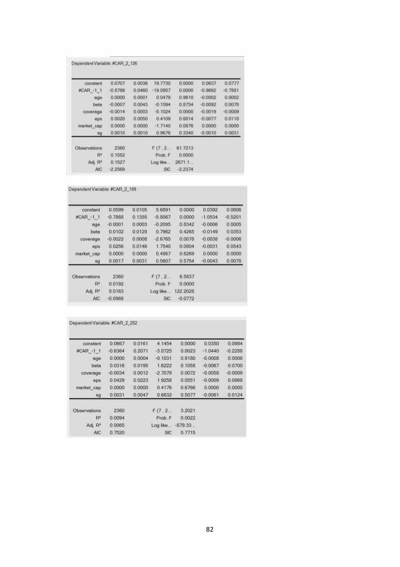
82

83
EAAR <0 SG

84

85
Appendix E: Robustness Check for other proxies
Table 14a - Robustness Check: EAAR/ES portfolios using EP as a proxy – Size Effect
Note: The values are represented in CAAR-values for each corresponding event window and post-event window based on the Size/BM classification portfolio. The significant levels are representing by: * for 10%, ** representing 5% and *** denotes for 1% under T1 Standardized Residual Test. If the values are in grey shaded then is either T2: Rank Test or T3 Generalized Sign Test, supporting the rejection. Every size/ proxy portfolio can be consulted in Appendix E
Table 14b - Robustness Check: EAAR portfolios using EP as a proxy – Size Effect
Note: The values are represented in CAAR-values for each corresponding event window and post-event window based on the Size/BM classification portfolio. The significant levels are representing by: * for 10%, ** representing 5% and *** denotes for 1% under T1 Standardized Residual Test. If the values are
Size_rank EP_rank obs MV (M £) EP EAAR (%) 1mth (%) 3mth (%) 6mth (%) 9mth (%) 1yr (%)
Small Glamour 1 28 204 -0.50 6.89*** 4.23 5.16 4.17 -2.97 -8.29
Small Value 5 51 830 0.18 5.54*** -0.89 -1.46 5.15 6.9 17.41**
Spread -1.35 -5.12 -6.62 0.98 9.87 25.7
Big Glamour 1 23 10657 0.03 3.77*** 1.09 0.63 -0.4 1.42 -0.84
Big Value 5 23 35883 0.15 3.03*** 0.34 1.7 2.14 2.57 2.6
Spread -0.74 -0.75 1.07 2.54 1.15 3.44
Small Glamour 1 141 181 -0.40 -8.89*** -5.32** -12.74*** -24.28*** -36.72*** -41.56***
Small Value 5 257 360 0.20 -7.06*** -1.64*** -8.29*** -9.48*** -12.72** -17.49***
Spread 1.83 3.68 4.45 14.8 24 24.07
Big Glamour 1 70 7976 0.02 -4.58*** -1.74* -6.39** -11.56** -13.13** -13.22*
Big Value 5 127 35609 0.12 -3.39*** -0.71* -2.87*** -3.27** -6.84*** -8.31***
Spread 1.19 1.03 3.52 8.29 6.29 4.91
Spread Small 14.43 4.43 11.28 29.43 43.62 58.97
Spread Big 7.61 2.08 8.09 13.7 15.7 15.82
Panel A: Earnings Surprise>0 & EAARs>0
Panel B: Earnings Surprise<0 & EAARs<0
Size_rank EP_rank obs MV (M £) EP EAAR (%) 1mth (%) 3mth (%) 6mth (%) 9mth (%) 1yr (%)
Small Glamour 1 185 146 -0.32 6.22*** 2.11* 1.65 4.79 0.54 1.54
Small Value 5 529 380 0.17 5.32*** 0.42 -0.44 0.48 -1.1 -1.29
Spread -0.9 -1.69 -2.09 -4.31 -1.64 -2.83
Big Glamour 1 151 7955 0.02 5.23*** -0.19 -0.78* 0.3 0.71 0.96
Big Value 5 190 33602 0.12 3.03*** -0.95** -0.41 -0.36 -0.47 0.56
Spread -2.2 -0.76 0.37 -0.66 -1.18 -0.4
Small Glamour 1 155 161 -0.39 -9.35*** -5.1** -14.13*** -26.54*** -40.96*** -49.71***
Small Value 5 318 371 0.21 -7.01*** -1.36*** -7.29** -8.08*** -11.35*** -14.75***
Spread 2.34 3.74 6.84 18.46 29.61 34.96
Big Glamour 1 90 7976 0.02 -4.78*** -0.64 -3.87* -7.07*** -9.84* -9.94*
Big Value 5 161 34887 0.12 -3.19*** -0.95*** -2.43*** -3.3*** -5.45** -6.54***
Spread 1.59 -0.31 1.44 3.77 4.39 3.4
Spread Small 14.67 5.52 13.69 27.02 39.86 48.42
Spread Big 7.81 -0.31 3.46 6.71 9.37 10.5
Panel A: EAARs>0
Panel B: EAARs<0

86
in grey shaded then is either T2: Rank Test or T3 Generalized Sign Test, supporting the rejection. Every size/ proxy portfolio can be consulted in Appendix E
Table 15a - Robustness Check: EAAR/ES portfolios using CP as a proxy – Size Effect
Note: The values are represented in CAAR-values for each corresponding event window and post-event window based on the Size/BM classification portfolio. The significant levels are representing by: * for 10%, ** representing 5% and *** denotes for 1% under T1 Standardized Residual Test. If the values are in grey shaded then is either T2: Rank Test or T3 Generalized Sign Test, supporting the rejection. Every size/ proxy portfolio can be consulted in Appendix E
Table 15b - Robustness Check: EAAR portfolios using CP as a proxy – Size Effect
Note: The values are represented in CAAR-values for each corresponding event window and post-event window based on the Size/BM classification portfolio. The significant levels are representing by: * for 10%, ** representing 5% and *** denotes for 1% under T1 Standardized Residual Test. If the values are
Size_rank CP_rank obs MV (M £) CP EAAR (%) 1mth (%) 3mth (%) 6mth (%) 9mth (%) 1yr (%)
Small Glamour 1 24 588 -0.11 5.44*** -1.07 -4.04* 0.85 -6.93* -9.96*
Small Value 5 40 647 0.41 7.09*** 2.38 5.68* 12.61** 15.59** 28.86**
Spread 1.65 3.45 9.72 11.76 22.52 38.82
Big Glamour 1 23 17761 0.01 3*** -0.57 -1.25 -2.17 -4.97 -6.96
Big Value 5 26 29049 0.16 3.87*** 0.98 5.44* 8.43** 14.63*** 18.48***
Spread 0.87 1.55 6.69 10.6 19.6 25.44
Small Glamour 1 87 359 -0.76 -8.36*** -0.45 -8.27* -11.58*** -17.03** -16.02**
Small Value 5 177 388 1.45 -6.7*** -2.38*** -11.02** -15.2*** -22.45*** -24.78**
Spread 1.66 -1.93 -2.75 -3.62 -5.42 -8.76
Big Glamour 1 70 147 0.01 -3.83*** -0.26 -2.5** -4.23*** -6.81*** -5.55***
Big Value 5 115 796 0.16 -3.91*** -1.11* -4.4*** -5.9* -7.24*** -10.59***
Spread -0.08 -0.85 -1.9 -1.67 -0.43 -5.04
Spread Small 15.45 2.83 13.95 24.19 32.62 44.88
Spread Big 7.7 1.24 7.94 12.66 21.44 24.03
Panel A: Earnings Surprise>0 & EAARs>0
Panel B: Earnings Surprise<0 & EAARs<0
Size_rank CP_rank obs MV (M £) CP EAAR (%) 1mth (%) 3mth (%) 6mth (%) 9mth (%) 1yr (%)
Small Glamour 1 111 356 -0.65 6.06*** -0.25 -1.94 -0.96 -7.02** -9.92**
Small Value 5 350 349 1.40 5.83*** 0.87 0.67 2.04 1.09 3.67
Spread -0.23 1.12 2.61 3 8.11 13.59
Big Glamour 1 151 12463 0.01 3.49*** -0.82** -1.14* -0.95 -2.71** -3.1**
Big Value 5 187 20526 0.16 3.98*** 0.27 1.56 1.08 1.73 2.95
Spread 0.49 1.09 2.7 2.03 4.44 6.05
Small Glamour 1 98 319 -0.73 -9.03*** -0.99 -10.83** -14.82*** -25.72* -30.7**
Small Value 5 226 349 1.46 -6.47*** -1.58** -8.98* -13.21*** -20.7*** -24.25***
Spread 2.56 -0.59 1.85 1.61 5.02 6.45
Big Glamour 1 90 12889 0.01 -3.81*** -0.52* -3.08*** -4.22* -6.21*** -5.42***
Big Value 5 158 21027 0.16 -3.66*** -0.89** -3.35*** -4.15* -4.92** -7.31**
Spread 0.15 -0.37 -0.27 0.07 1.29 -1.89
Spread Small 14.86 1.86 11.5 16.86 26.81 34.37
Spread Big 7.79 0.79 4.64 5.3 7.94 8.37
Panel A: EAARs>0
Panel B: EAARs<0

87
in grey shaded then is either T2: Rank Test or T3 Generalized Sign Test, supporting the rejection. Every size/ proxy portfolio can be consulted in Appendix E
Table 16a - Robustness Check: EAAR/ES portfolios using SG as a proxy – Size Effect
Note: The values are represented in CAAR-values for each corresponding event window and post-event window based on the Size/BM classification portfolio. The significant levels are representing by: * for 10%, ** representing 5% and *** denotes for 1% under T1 Standardized Residual Test. If the values are in grey shaded then is either T2: Rank Test or T3 Generalized Sign Test, supporting the rejection. Every size/ proxy portfolio can be consulted in Appendix E
Size_rank SG_rank obs MV (M £) SG EAAR (%) 1mth (%) 3mth (%) 6mth (%) 9mth (%) 1yr (%)
Small Value 1 26 546 -0.47 6.07*** 0.45 -0.75* 3.6 -0.46* 4.48
Small Glamour 5 47 642 0.94 5.38*** -1.14 0.12 1.49 2.92 4.91
Spread 0.69 1.59 -0.87 2.11 -3.38 -0.43
Big Value 1 23 22147 -1.01 2.8*** 0.05 2.15 4.06 1.41 4.14
Big Glamour 5 25 11931 0.28 3.39*** 0.31 0.73 1.48 2.44 2.84
Spread -0.59 -0.26 1.42 2.58 -1.03 1.3
Small Value 1 134 379 -0.53 -6.54*** -3.68*** -9.33*** -9.84* -12.95*** -14.87***
Small Glamour 5 248 486 0.73 -5.08*** -0.92 -6.51*** -10.36*** -13.49*** -16.61***
Spread -1.46 -2.76 -2.82 0.52 0.54 1.74
Big Value 1 71 26971 -0.84 -3.2*** 0.04 -1.76* -1.81 -1.89 -3.08*
Big Glamour 5 127 13996 1.77 -3.43*** -0.29 -1.78** -2.82** -4.97*** -5.03***
Spread 0.23 0.33 0.02 1.01 3.08 1.95
Spread Small 11.15 1.37 5.76 13.96 13.03 21.09
Spread Big 6.23 0.34 3.93 6.88 6.38 9.17
Panel A: Earnings Surprise>0 & EAARs>0
Panel B: Earnings Surprise<0 & EAARs<0

88
Table 16b - Robustness Check: EAAR portfolios using SG as a proxy – Size Effect
Note: The values are represented in CAAR-values for each corresponding event window and post-event window based on the Size/BM classification portfolio. The significant levels are representing by: * for 10%, ** representing 5% and *** denotes for 1% under T1 Standardized Residual Test. If the values are in grey shaded then is either T2: Rank Test or T3 Generalized Sign Test, supporting the rejection. Every size/ proxy portfolio can be consulted in Appendix E
Size_rank SG_rank obs MV (M £) SG EAAR (%) 1mth (%) 3mth (%) 6mth (%) 9mth (%) 1yr (%)
Small Value 1 176 362 -0.58 5.27*** 0.48 1.97 3.31 3.79 5.82*
Small Glamour 5 492 481 0.77 4.92*** 0.76* 0.07 1.25* 0.88 0.46
Spread 0.35 -0.28 1.9 2.06 2.91 5.36
Big Value 1 156 26184 -0.81 3.4*** -0.32 -0.16 0.19 -1.42 0.96
Big Glamour 5 189 13598 1.71 3.31*** -0.51 -0.71 -0.47 -0.12 1.18
Spread 0.09 0.19 0.55 0.66 -1.3 -0.22
Small Value 1 144 365 -0.62 -6.48*** -2.92** -8.49** -8.54*** -11.61* -13.57**
Small Glamour 5 303 484 0.72 -4.87*** -0.7 -5.21*** -8.07*** -11.65*** -14.88***
Spread -1.61 -2.22 -3.28 -0.47 0.04 1.31
Big Value 1 88 26971 -0.84 -3.11*** -0.23 -2.4* -2.25 -2.18 -3.74**
Big Glamour 5 160 13865 1.78 -3.21*** -0.34** -2.07*** -2.62*** -4.99*** -5.28***
Spread 0.1 0.11 -0.33 0.37 2.81 1.54
Spread Small 10.14 1.18 7.18 11.38 15.44 20.7
Spread Big 6.61 0.02 1.91 2.81 3.57 6.24
Panel A: EAARs>0
Panel B: EAARs<0