the rational numbers as an abstract data type

The Rational Numbers as an Abstract Data Type

J. A. BERGSTRA

University of Amsterdam, Informatics Institute, Amsterdam, The Netherlands

AND

J. V. TUCKER

University of Wales Swansea, Singleton Park, Swansea, United Kingdom

Abstract. We give an equational specification of the field operations on the rational numbers underinitial algebra semantics using just total field operations and 12 equations. A consequence of thisspecification is that 0−1 = 0, an interesting equation consistent with the ring axioms and manyproperties of division. The existence of an equational specification of the rationals without hiddenfunctions was an open question. We also give an axiomatic examination of the divisibility operator,from which some interesting new axioms emerge along with equational specifications of algebras ofrationals, including one with the modulus function. Finally, we state some open problems, including:Does there exist an equational specification of the field operations on the rationals without hiddenfunctions that is a complete term rewriting system?

Categories and Subject Descriptors: D.3.1 [Programming Languages]: Formal Definition and The-ory; D.3.3 [Programming Languages]: Language Constructs and Features; F.1.3 [Logics and Mean-ings of Programs]: Specifying and Verifying and Reasoning about Programs; F.3.2 [Logics andMeanings of Programs]: Semantics of Programming Languages; F.4.1 [Mathematical Logic andFormal Languages]: Mathematical Logic

General Terms: Verification, Languages

Additional Key Words and Phrases: Rational numbers, field, meadow, division-by-zero, total versuspartial functions, abstract data types, algebraic specification, equations, initial algebra, computablealgebras

ACM Reference Format:

Bergstra, J. A. and Tucker, J. V. 2007. The rational numbers as an abstract data type J. ACM54, 2, Article 7 (April 2007), 25 pages. DOI = 10.1145/1219092.1219095 http://doi.acm.org/10.1145/1219092.1219095

Authors’ addresses: J. A. Bergstra, University of Amsterdam, Informatics Institute, Kruislaan 403,1098 SJ Amsterdam, The Netherlands, e-mail: [email protected]; J. V. Tucker, Department of Com-puter Science, University of Wales Swansea, Singleton Park, Swansea, SA2 8PP, United Kingdom,e-mail: [email protected] to make digital or hard copies of part or all of this work for personal or classroom use isgranted without fee provided that copies are not made or distributed for profit or direct commercialadvantage and that copies show this notice on the first page or initial screen of a display along with thefull citation. Copyrights for components of this work owned by others than ACM must be honored.Abstracting with credit is permitted. To copy otherwise, to republish, to post on servers, to redistributeto lists, or to use any component of this work in other works requires prior specific permission and/ora fee. Permissions may be requested from Publications Dept., ACM, Inc., 2 Penn Plaza, Suite 701,New York, NY 10121-0701 USA, fax +1 (212) 869-0481, or [email protected]© 2007 ACM 0004-5411/2007/04-ART7 $5.00 DOI 10.1145/1219092.1219095 http://doi.acm.org/10.1145/1219092.1219095

Journal of the ACM, Vol. 54, No. 2, Article 7, Publication date: April 2007.

2 J. A. BERGSTRA AND J. V. TUCKER

1. Introduction

Measurements are made using some kind of gauge. To calibrate a gauge, onechooses a unit and divides that unit into a number k of subunits of equal size.Then a measurement is denoted by n whole units and m subunits or, in this case,n m

k = (nk + m)/k subunits. Note that measurements are finite.The set Q of rational numbers is a number system designed to denote measure-

ments. Most users make computations involving measurements. Hence, the set Qof rational numbers is among the truly fundamental data types. The rationals are thenumbers with which we make finite computations in practice. Despite the fact theyhave been known and used for over two millennia, they are somewhat neglected inthe modern theory of data types.

On the rationals, we calculate using standard operations such as the functions+, −, ·,−1. Algebras made by equipping Q with some selection of operations wecall here rational arithmetics. The algebra (Q | 0, 1, +, −, ·,−1 ) is usually calledthe field of rational numbers when the operations satisfy certain axioms.

In this article, we will model some rational arithmetics, including the field, asabstract data types. Now, the rationals can be specified by the field axioms; indeed,they are uniquely definable up to isomorphism as the prime subfield of characteristic0. However, the field axioms contain a negative conditional formula for inverse,which is difficult to apply and automate in formal reasoning. Specifically, we areinterested in finding equational specifications of rational arithmetics under initialalgebra semantics. Such equational axiomatisations allow simple term rewritingsystems for reasoning and computation. Surprisingly, after over 30 years of datatype theory, questions such as “Does there exist such an equational specificationwithout hidden functions of the field of rational numbers?” seem to be open.

According to our general theory of algebraic specifications for computable datatypes (e.g., Bergstra and Tucker [1982; 1983; 1987; 1995]), since the common ratio-nal arithmetics are computable algebras, they have various equational specificationsunder both initial and final algebra semantics. Computable rational arithmetics evenhave equational specifications that are also complete term rewriting systems (byBergstra and Tucker [1995]). However, these general specification theorems forcomputable data types involve hidden functions and are based on equationally de-finable enumerations of data. Recently, in Moss [2001], algebraic specificationsof the rationals were considered. Among several interesting observations, Mossshowed that there exists an equational specification with just one unary hiddenfunction. He used a special enumeration technique that reminds one of the generalmethods of Bergstra and Tucker [1995], but is based on a remarkable enumerationtheorem for the rationals in Calkin and Wilf [2000]. He also gave specifications ofrational arithmetics with a modulus operator and with a floor.

Here we prove:

THEOREM 1.1. There exists a finite equational specification under initial alge-bra semantics, without hidden functions, of the rational numbers with field opera-tions that are all total.

Our axioms include the commutative ring axioms and some general rules forinverses from which it can be deduced that

0−1 = 0.


The Rational Numbers as an Abstract Data Type 3

This equation is also true of the hidden function specification in Moss [2001]. Theequation 0−1 = 0 occurs in several other places as well, for reasons of technicalconvenience (e.g., Hodges [1993] and Harrison [1998]). Our proposed specificationincludes a special axiom that codes a representation of an infinite subset of positiverational numbers.

The pursuit of this result leads to a thorough axiomatic examination of the divis-ibility operator, in which some interesting new axioms and models are discovered.In particular, we introduce a class of commutative rings with interesting divisionproperties, which we call meadows.

The structure of the article is this: In Section 2, we give the basic equations thatdefine the rational arithmetic operations and define some of their properties. InSection 3, we give two equational specifications of the rational field without hiddenfunctions, one recursive and infinite, and one finite. In Section 5, we give resultson fields and equational subtheories of fields, and on other rational arithmetics.Finally, in Section 6, we discuss some open problems.

This article is the first of a series on equational specifications of the rational arith-metics and their extensions, see Bergstra and Tucker [2006a; 2006b] and Bergstra[2006], launched in 2005 by Bergstra and Tucker [2005]. It can be read as a se-quel to Bergstra and Tucker [1987; 1995], which contains a literature survey andthe complementary general results. We use only the basic ideas of initial algebraspecification. However, with several unfamiliar axioms about the familiar inverseoperator in action, care is needed in verifying equations and other formulae.

We thank Kees Middelburg, Yoram Hirschfeld and an anonymous referee forvaluable comments on the subject.

2. Axioms for Rational Arithmetic

2.1. PRELIMINARIES ON ALGEBRAIC SPECIFICATIONS. We assume the reader isfamiliar with using equations and conditional equations and initial algebra seman-tics to specify data types. Some accounts of this are: Goguen et al. [1978], Meseguerand Goguen [1985], and Wirsing [1990].

The theory of algebraic specifications is based on theories of universal algebras(e.g., Wechler [1992] and Meinke and Tucker [1992]); computable and semicom-putable algebras [Stoltenberg-Hansen and Tucker 1995]; and term rewriting [Klop1992; Terese 2003].

We use standard notations: typically, we let � be a many sorted signature andA a total � algebra. The class of all total � algebras is Alg(�) and the class ofall total � algebras satisfying all the axioms in a theory T is Alg(�, T ). The word“algebra” will mean total algebra.

2.2. ALGEBRAIC SPECIFICATIONS OF THE RATIONALS. We will build ourspecifications in stages. The primary signature � is simply that of the field ofrational numbers:

signature �sorts fieldoperations0: → field;1 : → field;



+ : field × field → field;− : field → field;· : field × field → field;−1 : field → fieldend

The first set of eight axioms is that of a commutative ring with 1, whichestablishes the standard properties of +, −, and ·. We will refer to these axiomsby CR1, . . . , CR8.

equations CR

(x + y) + z = x + (y + z)x + y = y + xx + 0 = x

x + (−x) = 0(x · y) · z = x · (y · z)

x · y = y · xx · 1 = x

x · (y + z) = x · y + x · z

end

Our first set SIP of axioms for −1 contain the following, which we call thestrong inverse properties. They are “strong” because they are equations involving−1 without any guards, such as x �= 0:

equations SIP

(−x)−1 = −(x−1)(x · y)−1 = x−1 · y−1

(x−1)−1 = x

end

We will refer to these axioms by SIP1, . . . ,SIP3. The set CR ∪ SIP ofequations and its extensions are our basic object of study. We will also need otheraxioms, especially about −1.

Later, we will add to CR ∪ SIP the restricted inverse law (Ril),

x · (x · x−1) = x ,

which, using commutativity and associativity, expresses that x · x−1 is 1 in thepresence of x .

Hirschfeld (Personal Communication 2006) has shown that equations SIP1 andSIP2 are derivable from SIP3 using CR ∪Ril.

The standard axioms of a field simply add to CR the following: the generalinverse law (Gil)



x �= 0 =⇒ x · x−1 = 1

and the axiom of separation (Sep)

0 �= 1.

Guarded versions of the equations of SIP—such as, x �= 0 =⇒ (x−1)−1 = x—canbe proved from Gil and Sep.

2.3. TOTALIZED FIELDS AND ALGEBRAS SATISFYING THE SPECIFICATIONS.Let us consider the notion of a field in our setting. Let (�, Tfield) be the axiomaticspecification of fields, where

Tfield = CR ∪ Gil ∪ Sep.

The class Alg(�, Tfield) is the class of total algebras satisfying the axioms in Tfield.For emphasis, we refer to these algebras as totalized fields.

For all totalized fields A ∈ Alg(�, Tfield) and all x ∈ A, the inverse x−1 is defined.In particular, 0−1

A is defined. What can it be?Now suppose 0−1

A = a for some a ∈ A. Then, we must expect that

0−1A · 0A �= 1A.

To see this, note that a · 0A = 0A for all a in a ring (see Lemma 2.1(a) below). So0−1

A · 0A = 0A and 0A �= 1A by Sep. Thus, at this stage, the actual value 0−1A = a

can be anything. Choosing 0−1A = a we may speak of an a-totalized field and, in

particular, when a = 0 of a 0-totalized field.Now, the axiomatic theory of fields is one of the central topics in the model theory

of first order languages: it has shaped the subject and led to its best applications.In model theory operations in signatures are invariably total. It is common to ax-iomatise fields using a set of �2 sentences over the ring signature thus avoiding thequestion of the totality of the inverse operation. However, with this ring signature,the substructures are rings and not necessarily fields. Thus, axiomatisations basedon the field signature with the following axiom are also used (see, e.g., Hodges[1993, p. 695])

0−1 = 0 ∧ x �= 0 =⇒ x · x−1 = 1.

In fact, 0 is a common choice for the value of 0−1. In automated reasoning, forexample, Harrison [1998] used 0−1 = 0 and observed that SIP1, SIP2 and SIP3 arevalid in the 0-totalised reals.

Our own interest will be in the specification CR ∪ SIP. Shortly, we shall showthat this specification will force the choice of 0−1 = 0.

The main �-algebra we are interested in is

Q0 = (Q | 0, 1, +, −, ·,−1 )

where the inverse is total

x−1 = 1/x if x �= 0;= 0 if x = 0.



This total algebra satisfies the axioms of a field Tfield and is a 0-totalized field ofrationals.

Similarly, we can define the a-totalized field Qa of rationals where the inverseis made total by 0−1 = a.

2.4. PROPERTIES. We will now derive some simple equational properties fromthe axioms.

LEMMA 2.1. The following equations are provable from CR:(a) 0 · x = 0.(b) (−1) · x = −x.(c) (−x) · y = −(x · y).(d) −0 = 0.(e) (−x) + (−y) = −(x + y).(f) −(−x) = x.

PROOF(a) We calculate:

0 + 0 = 0 by CR3(0 + 0) · x = 0 · x multiplying both sides by x

0 · x + 0 · x = 0 · x by CR8 and CR6(0 · x + 0 · x) + (−(0 · x)) = 0 · x + (−(0 · x)) adding to both sides0 · x + (0 · x + (−(0 · x))) = 0 by CR1 and CR4

0 · x + 0 = 0 by CR40 · x = 0 by CR3.

(b) We calculate:

(−1) · x = (−1) · x + (x − x) by CR3 and CR4= ((−1) · x + (x · 1)) − x by CR7 and CR1= ((−1) · x + (1 · x)) − x by CR6= ((−1) + 1) · x − x by CR8= (1 + (−1)) · x − x by CR2= 0 · x − x by CR4= 0 − x by this Lemma clause (a)= −x by CR3.

(c) We calculate:

(−x) · y = ((−1) · x) · y by this Lemma clause (b)= (−1) · (x · y) by CR5= −(x · y) by this Lemma clause (b).

(d) We calculate:

−0 = (−1) · 0 by this Lemma clause (b)= 0 by this Lemma clause (a).



(e) We calculate:

(−x) + (−y) = 0 + ((−x) + (−y)) by CR3= (−(x + y) + (x + y)) + ((−x) + (−y)) by CR3= −(x + y) + ((x + −x) + (y + −y)) by CR1 and CR2= −(x + y) + (0 + 0) by CR4= −(x + y) + 0 by CR3= −(x + y) by CR3.

(f) We calculate:

−(−x) = 0 + −(−x) by CR3= (x + (−x)) + −(−x) by CR4= x + ((−x) + −(−x)) by CR1= x + 0 by CR3= x by CR3. �

We know from (a) that 0 = 0 · 0−1 is valid in a commutative ring. On adding theaxioms SIP to CR, we force a value for 0−1:

THEOREM 2.2. The following equation is provable from CR ∪ SIP:

0−1 = 0.

PROOF. First observe that:

0 = 0−1 + −(0−1) by CR4

= 0−1 + (−0)−1 by SIP1

= 0−1 + 0−1 by Lemma 2.1(d).

Now we calculate:

0−1 = (0−1 + 0−1)−1 by applying −1

= (1 · 0−1 + 1 · 0−1)−1 by CR6 and CR7

= ((1 + 1) · 0−1)−1 by CR8

= (1 + 1)−1 · (0−1)−1 by SIP2

= (1 + 1)−1 · 0 by SIP3= 0 by Lemma 2.1(a) and CR2.

2.5. EQUATIONAL SUBTHEORIES OF FIELDS. Given the three axioms of SIP,one might ask: What is wrong with the unguarded equation x · x−1 = 1? It is easyto show that it contradicts Sep, that is,

CR ∪{x · x−1 = 1} 0 = 1.

So we must try other equations for inverse. The axiom Ril implies a wider contextfor inverse.

LEMMA 2.3. CR ∪ SIP ∪Ril u · x · y = u =⇒ u · x · x−1 = u.



PROOF. We calculate:

u · x · x−1 = (u · x · y) · x · x−1 by premiss

= u · y · x · x · x−1 by commutativity= u · y · x by Ril= u by premiss. �

Let us show that the equational specifications are (almost) subtheories of Tfield =CR ∪ Gil ∪ Sep. First, we need this cancelation lemma:

LEMMA 2.4. Tfield x · y = 1 ∧ x · z = 1 → y = z.

PROOF. If x · y = 1, then x �= 0. Multiply both assumptions by x−1 and we havex−1 · x · y = x−1 and x−1 · x · z = x−1. So, using Gil for x �= 0, we have 1 · y = x−1

and 1 · z = x−1. By CR7, we have y = x−1 = z. �

LEMMA 2.5. Tfield ∪ {0−1 = 0} SIP and Tfield ∪ {0−1 = 0} Ril.

PROOF. Consider the three axioms of SIP in turn.(1) (−x)−1 = −(x−1). If x = 0, then the equation is true trivially. Suppose x �= 0

and so −x �= 0. We calculate:

1 = (−x) · (−x)−1 by Gil

= (−1 · x) · (−x)−1 by Lemma 2.1(b)

= x · −1 · (−x)−1 by CR6

= x · −(−x)−1 by Lemma 2.1(b).

By Gil, we also have 1 = x · x−1. So,

x−1 = −(−x)−1 by Cancellation Lemma 2.4

−(x−1) = −(−(−x)−1) by applying −= (−x)−1 by Lemma 2.1(f).

(2) (x · y)−1 = x−1 · y−1. If x = 0 or y = 0, then the equation is true trivially. Ifx �= 0 and y �= 0, then x · y �= 0. By Gil, we have

(x · y) · (x · y)−1 = 1

and by the axioms of CR

(x · y) · x−1 · y−1 = 1 · 1 = 1.

Thus, by cancellation, (x · y)−1 = x−1 · y−1.(3) (x−1)−1 = x . If x = 0, then the equation is true trivially. If x �= 0, then

x−1 �= 0. By Gil, we have

(x−1) · (x−1)−1 = 1 and (x−1) · x = 1.

By cancellation, (x−1)−1 = x .The derivation of Ril is obvious. �



Notice that for any closed equation, Tfield t = s implies Tfield ∪ {0−1 = 0} t = s, which is trivial as is monotonic.

3. Initial Algebra Specification

We give two algebraic specifications of the rationals, one infinite and one finite.

3.1. A RECURSIVE EQUATIONAL SPECIFICATION. Let us define the numeralsover � by 0 = 0 and n + 1 = n + 1. We denote 0, 1, 1 + 1, (1 + 1) + 1, . . . by0, 1, 2, 3, . . . . Now we define a set I of closed �-equations between numerals by

I = {n · (n)−1 = 1 | n > 0}.THEOREM 3.1. There exists a recursive equational initial algebra specification

(�, CR ∪ SIP ∪ I ), without hidden functions, of the totalised field Q0 of rationalnumbers, that is,

T (�, CR ∪ SIP ∪ I ) ∼= Q0.

PROOF. Clearly, the specification I is decidable. Note that, by inspection,

Q0 |= CR ∪ SIP ∪ I .

By initiality, there exists a unique �-homomorphism φ : T (�, CR ∪ SIP ∪ I )→ Q0.

As Q0 is �-minimal, we know that φ is surjective. Thus, to complete the proof,we must show that φ is also injective.

Consider Q0. The domain Q of Q0 can be represented as follows:

Q = {0} ∪ { nm | n > 0, m > 0, gcd(n, m) = 1

}∪ { − n

m | n > 0, m > 0, gcd(n, m) = 1}.

We use this representation to calculate the values of φ on certain equivalence classesof terms in T (�, CR ∪ SIP ∪ I ):

LEMMA 3.2. The following hold:φ([0]) = 0φ([1]) = 1φ([n]) = nφ([n−1]) = 1

nφ([n · m−1]) = n

m , providing gcd(n, m) = 1.φ([−(n · m−1)]) = − n

m , providing gcd(n, m) = 1.

PROOF. Cases (i) and (ii) are obvious since φ preserves constants. Case (iii)is shown by induction on n. Case (iv) is shown by induction on n and uses theinterpretation of −1. The last two cases are based on

φ([n · m−1]) ={

φ([n])φ([m]) if gcd(n, m) = 1;n:gcd(n,m)m:gcd(n,m) otherwise

where we use: to denote division on natural numbers. �



These observations suggest the following definition and lemma. Let

T R = {0} ∪ {n · m−1 | n > 0, m > 0, gcd(n, m) = 1}∪ {−(n · m−1) | n > 0, m > 0, gcd(n, m) = 1}.

LEMMA 3.3. The set TR is a transversal for the equivalence relation ≡CR∪SIP∪I ,that is, each equivalence class contains one and only one element of TR.

Before we prove Lemma 3.3, let us note that it is enough to prove φ is injective.For suppose

φ([t]) = φ([t ′]).

Then, by Lemma 3.3, we know that [t] = [r ] and [t ′] = [r ′] for unique r, r ′ ∈ TR.Thus,

φ([r ]) = φ([r ′]).

But, by Lemma 3.2, we know that φ([r ]) and φ([r ′]) have values in the normal formof n

m , or − nm , provided gcd(n, m) = 1, etc. This happens if, and only if, r = r ′ and

hence if, and only if, [t] = [t ′].It remains to prove the Lemma 3.3 as follows:PROOF. Let E = CR ∪ SI P ∪ I . We have to show that:

(1) for each closed term t ∈ T (�) there is some u ∈ T R such that E t = u;(2) for any closed terms k, l ∈ T R, if E k = l then k ≡ l.

The proof of (1) is by induction on the structure of term t and requires a largecase analysis based on the leading function symbol of t in � and possible normalforms for subterms in TR. We give one of the induction cases for illustration:

Case: Multiplication t = r · s.By induction, both r and s are provably equivalent to elements of TR. We take

the following subcase: suppose

(�, E) r = n · m−1 and E s = −(k · l−1).

Now,

(�, E) r · s = n · m−1 · −(k · l−1) by substitution

r · s = n · m−1 · (−1) · (k · l−1) by CR6 and CR7

r · s = (−1) · n · m−1 · k · l−1 by CR8

r · s = (−1) · (n · k) · (m−1 · l−1) by SIP2

r · s = (−1) · (n · k) · (m · l)−1 by SIP3

r · s = (−1) · (n.k) · (m.l)−1 by SIP3

r · s = −(n.k) · (m.l)−1 by SIP3.



Now let u = gcd(n.k, m.l). If u = 1, then we are done. Suppose that n.k = u.pand m.l = u.q and so gcd(p, q) = 1. Then we continue rewriting:

(�, E) r · s = −(u.p) · (u.q)−1 by definition

r · s = −(u · p) · (u · q)−1 by Lemma 3.4

r · s = −(u · u−1)(p · q−1) by CR6 and SIP2

r · s = −p · q−1 by equations of I.

The term −p ·q−1 is of the required form because gcd(p, q) = 1. The followingis an easy induction.

LEMMA 3.4. For any p, q ∈ N we have

(�, E) p + q = p + q(�, E) p.q = p · q(�, E) −p = −p.

The proof of uniqueness condition (2) is easy: Suppose k �= l. Then they havedifferent interpretations in Q0 under φ. This means that they cannot be proved equalby the axioms CR ∪ SIP ∪ I since Q0 satisfies these axioms.

This completes the proof of Lemma 3.3 and hence the proof of Theorem 3.1. �

3.2. A FINITE EQUATIONAL SPECIFICATION. We first introduce an operation:

Definition 3.5. Z (x) = 1 − x · x−1.

The operator “measures” the difference between x · x−1 and 1. Clearly,

Z (x) = 0 ⇔ x · x−1 = 1.

The operator has many useful properties. For example, the set I of closed equa-tions used in Section 3.1 can be written

I = {Z (n) = 0 | n > 0}.The operator Z is a function that is definable by a term over the field signature. Itis used to simplify notations and calculations below. It does not count as a hiddenfunction as it can be simply removed from all specifications by expanding its explicitdefinition.

Recall Lagrange’s Theorem that every natural number can be represented asthe sum of four squares (see Dickson [1952, pp. 275–303]). We define a specialequation L (for Lagrange):

Z (1 + x2 + y2 + z2 + u2) = 0.

L expresses that for a large collection of numbers (in particular, those q which canbe written as 1 plus the sum of four squares) q · q−1 equals 1.

THEOREM 3.6. There exists a finite equational initial algebra specification,without hidden functions, of the totalised field Q0 of rational numbers; in particular,



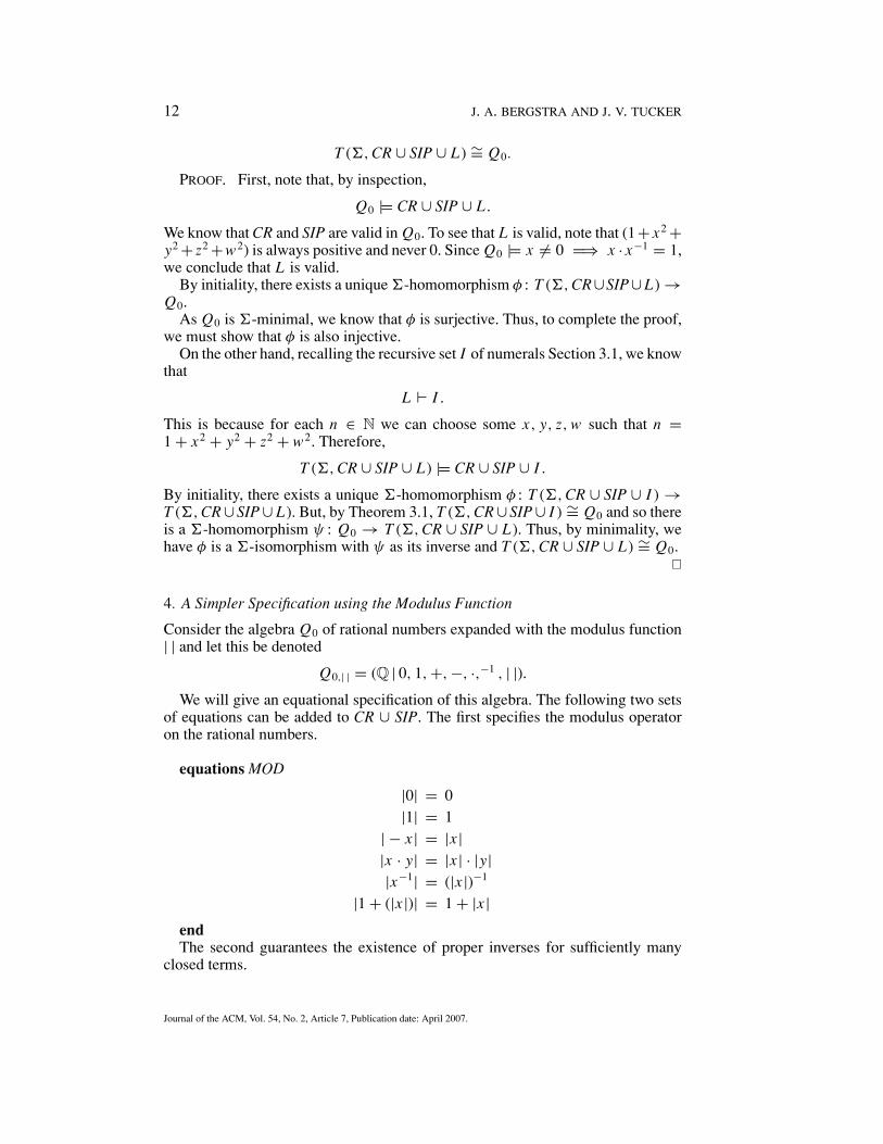
T (�, CR ∪ SIP ∪ L) ∼= Q0.

PROOF. First, note that, by inspection,

Q0 |= CR ∪ SIP ∪ L .

We know that CR and SIP are valid in Q0. To see that L is valid, note that (1+ x2 +y2 + z2 +w2) is always positive and never 0. Since Q0 |= x �= 0 =⇒ x · x−1 = 1,we conclude that L is valid.

By initiality, there exists a unique �-homomorphism φ : T (�, CR∪SIP∪ L) →Q0.

As Q0 is �-minimal, we know that φ is surjective. Thus, to complete the proof,we must show that φ is also injective.

On the other hand, recalling the recursive set I of numerals Section 3.1, we knowthat

L I .

This is because for each n ∈ N we can choose some x, y, z, w such that n =1 + x2 + y2 + z2 + w2. Therefore,

T (�, CR ∪ SIP ∪ L) |= CR ∪ SIP ∪ I .

By initiality, there exists a unique �-homomorphism φ : T (�, CR ∪ SIP ∪ I ) →T (�, CR ∪ SIP ∪ L). But, by Theorem 3.1, T (�, CR ∪ SIP ∪ I ) ∼= Q0 and so thereis a �-homomorphism ψ : Q0 → T (�, CR ∪ SIP ∪ L). Thus, by minimality, wehave φ is a �-isomorphism with ψ as its inverse and T (�, CR ∪ SIP ∪ L) ∼= Q0.

�

4. A Simpler Specification using the Modulus Function

Consider the algebra Q0 of rational numbers expanded with the modulus function| | and let this be denoted

Q0,| | = (Q | 0, 1, +, −, ·,−1 , | |).We will give an equational specification of this algebra. The following two sets

of equations can be added to CR ∪ SIP. The first specifies the modulus operatoron the rational numbers.

equations MOD

|0| = 0|1| = 1

| − x | = |x ||x · y| = |x | · |y||x−1| = (|x |)−1

|1 + (|x |)| = 1 + |x |endThe second guarantees the existence of proper inverses for sufficiently many

closed terms.



equations Modril

Z (1 + |x |) = 0

end

To get used to the axioms for | |, we prove a simple lemma of use later:

LEMMA 4.1. For each k ∈ N, CR ∪ MOD |k| = k.

PROOF. By induction on k.Basis, k = 0: We calculate:

|0| = |0| by definition of 0= 0 by MOD1= 0 by definition of 0.

Induction step, k + 1, Assume as induction hypothesis that |k| = k. We calculate:

k + 1 = k + 1 by definition of k + 1= 1 + k by commutativity CR2= 1 + |k| by induction hypothesis= |1 + |k|| by MOD6= |1 + k| by induction hypothesis= |k + 1| by CR2 and the definition of k + 1. �

THEOREM 4.2. The initial algebra T (� ∪ {||}, CR ∪ SIP ∪ MOD ∪ Modril) isisomorphic to the algebra Q0,| | of rational numbers.

PROOF. The proof follows the pattern of earlier theorems (Theorems 3.1 and3.6). For notational convenience, let

E = CR ∪ SIP ∪ MOD ∪ Modril.

The equations in E are valid in Q0,| |. Thus, by initiality, there exists a unique� ∪ {| |}-homomorphism

ψ : T (� ∪ {| |}, E) → Q0,| |.

As Q0,| | is � ∪ {| |}-minimal, we know that ψ is surjective. Thus, to complete theproof, we must show that ψ is also injective.

The carrier of Q0,| | is the same as Q0 and is

Q = {0} ∪ { nm | n > 0, m > 0, gcd(n, m) = 1

}∪ { − n

m | n > 0, m > 0, gcd(n, m) = 1}.

This suggests that we should use the previous transversal

T R = {0} ∪ {n · m−1 | n > 0, m > 0, gcd(n, m) = 1}∪ {−(n · m−1) | n > 0, m > 0, gcd(n, m) = 1}.

as a transversal for T (� ∪ {| |}, E). Following the pattern of Theorem 3.1, we canprove new versions of the evaluation and transversal Lemmas 3.2 and 3.3.



First, we generalize the numeral notation for the naturals to a notation for therationals. For each r ∈ Q, we define

r = 0 if r = 0;

= n · m−1 if r = nm

and n > 0, m > 0, gcd(n, m) = 1

= −(n · m−1) if r = − nm

and n > 0, m > 0, gcd(n, m) = 1

Thus, with this notation, T R = {r | r ∈ Q}.LEMMA 4.3. The � ∪{| |} homomorphism ψ satisfies ψ([r ]) = r for all r ∈ Q.

PROOF. This follows the same arguments as the proof of Lemma 3.2. Note clauses(i), (v) and (vi). �

LEMMA 4.4. The set TR is a transversal for the equivalence relation ≡E onT (� ∪ {| |}).

Suppose we have proved this fact, then we can conclude the proof of the theoremas follows. If

ψ([t]) = ψ([t ′]),

then, by Lemma 4.4, there exist r , r ′ ∈ TR such that

E t = r and E t ′ = r ′.

Thus,

ψ([r ]) = ψ([r ′]).

Now, by Lemma 4.3,

ψ([r ]) = r and ψ([r ′]) = r ′.

Thus,

r = r ′.

Since TR is a transveral, this happens if, and only if, the terms

r = r ′

and hence [r ] = [r ′] and [t] = [t ′].

It remains to prove Lemma 4.4. We note the following.

LEMMA 4.5. CR ∪ MOD ∪ Modril I

PROOF. We can write the set I as

I = {Z (n) = 0 | n > 0}and so prove, by induction on n > 0, that CR ∪ MOD ∪ Modril Z (n) = 0.



Basis n = 1. We calculate:

Z (1) = Z (1 + 0) by CR3 and the definition of 0= Z (1 + |0|) by MOD1= 0 by Modril.

Induction Step n = k + 1. We calculate:

Z (k + 1) = Z (k + 1) by the definition of k + 1= Z (1 + k) by CR2= Z (1 + |k|) by Lemma 4.1= 0 by Modril. �

We can show that for every term t ∈ T (� ∪ {| |}) there is an r ∈ T R such thatE t = r . Notice that by Lemma 4.5, and Lemma 3.3, we know that for all termst not containing | |, t ∈ T (�), E t = r .

We prove the transversal lemma by induction on the height Ht(t) of terms t ∈T (� ∪ {| |}).

Basis. Ht(t) = 0. Then t = 0 or t = 1 and we are done.Induction Step, Ht(t) = k + 1. Suppose that the lemma is true for terms of

height lower than Ht(t) = k and consider a term of height k. There are five casescorresponding to the operations. We consider two for illustration.

Case t = s + s ′. By induction,

E s = r and E s ′ = r ′

for r , r ′ ∈ T R. Thus,

E s + s ′ = r + r ′.

Now r + r ′ does not contain | | and so reduces to some element in TR.Case t = |s|. This is the interesting case. By induction, E s = r . There are

three subcases.If r = 0, then t = |r | = |0| = 0 by MOD1.If r = n · m−1, then

t = |n · m−1| by definition

= |n| · |m−1| by MOD4

= |n| · |m|−1 by MOD5

= n · m−1 by Lemma 4.1.

If r = −(n · m−1), then

t = | − (n · m−1)| by the definition

= n · m−1 by MOD3. �



The specification CR ∪ SIP ∪ MOD ∪ Modril of the rational numbers is simplerthan the specification CR ∪ SIP ∪ L because it does not depend on (somewhat)sophisticated number theory.

5. Specifications of Totalized Fields and Other Rational Arithmetics

5.1. ON THE EQUATIONAL THEORY OF TOTALIZED FIELDS. It has long beenknown that the class of totalised fields is not a variety, that is, is not definable byequations over the field signature. The argument is based on the fact that the classof totalised fields is not closed under products (compare Birkhoff’s Theorem, see,e.g., Meinke and Tucker [1992]).

We can rephrase and reprove this elementary fact in the present setting as follows:

LEMMA 5.1. There is no set E of equations over the signature � of fields thatis logically equivalent with CR ∪ SIP ∪ Sep ∪ Gil.

PROOF. Assume the contrary and suppose that there is such a set of equations Esuch that Alg(�, E) = Alg(�, CR ∪ SIP ∪ Sep ∪ Gil). Consider the initial algebraI (�, E) of E . Now because the �-algebra Q0 of rational numbers is a model ofE , we know that

I (�, E) |= ¬(1 + 1 = 0).

To see this, note that if 1 + 1 = 0 was valid in the initial model I (�, E) in thenit would be valid under every homomorphism and, in particular, would be valid inQ0, which it is not.

Now, by assumption, I (�, E) |= CR ∪ SIP ∪ Sep ∪ Gil and this implies

I (�, E) |= Z (1 + 1) = 0.

But the prime totalized field Z2 of characteristic 2 is also a model of CR ∪ SIP ∪Sep ∪ Gil. By initiality, here is an unique homomorphism φ : I (�, E) → Z2 and,being a minimal structure, Z2 must be a homomorphic image of I (�, E). Now sinceZ (x) is a term, φZ (a) = Z (φ(a)) for all a ∈ A and φ(Z (1 + 1)) = Z (φ(1 + 1)) =Z (φ(1)+φ(1)) = Z (1+1). In Z2, we have 1+1 = 0, which implies Z (1+1) = 1.Thus, the unique homomorphism φ maps Z (1+1) = 0 in I (�, E) to Z (1+1) = 1in Z2, which is impossible for a homomorphism since the algebras satisfy Sep. (Infact, more generally all homomorphisms between fields must be injective.) This isa contradiction. �

Using a similar argument one can prove that there is no conditional equationaltheory C E over the signature � of fields which is equivalent to CR ∪ SIP ∪ Sep ∪Gil in first order logic.

5.2. THE RESTRICTED INVERSE LAW. Recall Ril is

x · (x · x−1) = x .

In the presence of CR ∪ SIP, another way of writing Ril is as follows:

Z (x) · x = 0.



We will now use the equational specification (�, CR ∪ SIP ∪ Ril). If one restrictsattention to the closed equations over �, an interesting positive result is found(Theorem 5.6).

Now Ril is derivable from CR ∪ SIP ∪ Sep ∪ Gil and for that reason CR ∪ SIP ∪Ril is a weaker theory than CR ∪ SIP ∪ Sep ∪ Gil. Of course, the key point is thatCR ∪ SIP ∪ Ril is an equational theory over � in which inverses are possible.

To illustrate further the implications of Ril, here is a listing of identities that caneasily be proved from CR ∪ SIP ∪ Ril:

LEMMA 5.2. The following equations can be proved from CR ∪ SIP ∪ Ril

Z (0) = 1Z (1) = 0

Z (x) · Z (x) = Z (x)(Z (x))−1 = Z (x)

(1 − Z (x)) · (1 − Z (x)) = 1 − Z (x)(1 − Z (x))−1 = 1 − Z (x).

PROOF. Equations (1) and (2) are obvious in any commutative ring. The othercases are calculations; we do the remaining cases.

Consider Z (x) · Z (x) = Z (x).

Z (x) · Z (x) = (1 − x · x−1) · (1 − x · x−1)

= 1 − x · x−1 − x · x−1 + (x · x−1) · (x · x−1)

= 1 − x · x−1 − x · x−1 + (x · x−1 · x) · x−1

= 1 − x · x−1 − x · x−1 + x · x−1 by Ril

= 1 − x · x−1

= Z (x).

Consider Z (x)−1 = Z (x).

Z (x)−1 = Z (x)−1 · (Z (x)−1 · Z (x)) by Ril

= (Z (x) · Z (x))−1 · Z (x) by SIP

= Z (x)−1 · Z (x) by above

= Z (x)−1 · Z (x) · Z (x) by above= Z (x).

Consider (1 − Z (x)) · (1 − Z (x)) = 1 − Z (x).

(1 − Z (x)) · (1 − Z (x)) = 1 − Z (x) − Z (x) + Z (x) · Z (x) by expansion= 1 − Z (x) − Z (x) + Z (x) by above= 1 − Z (x).



Consider (1 − Z (x))−1 = 1 − Z (x).

(1 − Z (x))−1 = (1 − (1 − x · x−1))−1 by expansion

= (x · x−1)−1

= x−1 · (x−1)−1 by CR

= x−1 · x by CR

= x · x−1

= (1 − (1 − x · x−1))= 1 − Z (x). �

LEMMA 5.3. Let p, q be different prime numbers. Then

CR ∪ SIP ∪ Ril Z (p) · Z (q) = 0.

PROOF. Let a, b ∈ Z be such that 1 = a · p+b·q. There are different cases of whichwe will do one. Assume a = n and b = −m for n, m ∈ N. Then 1 = n · p − m · q .We calculate:

Z (p) = Z (p) · 1 by multiplying

= Z (p) · (n · p − m · q) by substituting

= Z (p) · n · p − Z (p) · m · q by SIP

= Z (p) · p · n − Z (p) · q · m by above

= 0 · n − Z (p) · q · m by Ril

= Z (p) · q · −m.

By Lemma 2.3, we have Z (p) = Z (p) · q · q−1. Thus, Z (p) · (1 − q · q−1) = 0 andthis is Z (p) · Z (q) = 0.

LEMMA 5.4. For each prime p and closed term t ∈ �, there is a unique naturalnumber n < p such that

CR ∪ SIP ∪ Ril Z (p) · t = Z (p) · n.

PROOF. This is proved by an induction on the structure of t .Basis. If t ≡ k then write k = n + p · l for natural numbers n and l with n < p.

Now

Z (p) · k = Z (p) · n + p · l by substitution

= Z (p) · n + Z (p) · p · l by CR

= Z (p) · n by Ril.

Induction Step. There are four cases corresponding with +, −, ·,−1 of which wewill do one for illustration.



Let t ≡ r−1 then we calculate:

Z (p) · t = Z (p) · r−1 by substitution

= Z (p) · Z (p) · r−1 by Lemma 5.2

= Z (p) · (Z (p))−1 · r−1 by Lemma 5.2

= Z (p) · (Z (p) · r )−1 by SIP

= Z (p) · (Z (p) · n)−1 by induction

= Z (p) · (Z (p))−1 · n−1 by SIP

= Z (p) · n−1 by Lemma 5.2

= Z (p) · m with m < p such that m = n−1 mod p.

That the number n is unique follows from an inspection of the prime field ofcharacteristic p. In that field Z (p) equals 1 while different numerals n1 and n2 withn1 and n2 both below p have different interpretations.

By inspection, we can check the following refinement of the statement of thelemma.

COROLLARY 5.5. Let val0p(t) the value of term t in the totalised field K 0

p. Theunique number n is val0

p(t). Therefore, we have

CR ∪ SIP ∪ Ril Z (p) · t = Z (p) · val0p(t).

The following theorem states that the equational subtheory T 0field can prove all the

closed identities that are true in all fields.

THEOREM 5.6. For any closed terms t, t ′ ∈ T (�), we have

T 0field t = t ′ implies CR ∪ SIP ∪ Ril t = t ′

Recall that if Tfield t = t ′ then T 0field t = t ′.

PROOF. The proof is rather involved with many calculations needed to establishcanonical forms. The canonical forms depend on the characteristics of the totalizedfields.

Let pn represent an enumeration of the primes in increasing order, starting withp0 = 2. Then, we define the following special terms:

G1 = 1, G2 = 1 − Z (p1), Gn+1 = Gn · (1 − Z (pn)).

For each n, the term Gn equals 0 in any prime field K 0pn

with characteristic pn orless. For all n, the term Gn equals 1 in any field of characteristic 0 and, in particular,in the totalized field of rational numbers.

LEMMA 5.7. For all n, we have:(i) Gn = 1 − Z (p1) − · · · − Z (pn−1).(ii) Gn · Z (pn) = Z (pn)

(iii) if n ≤ m, then Gm · Gn = Gm(iv) if k < pn, then Gn · k · k−1 = Gn.

PROOF. Exercise.



Using these G terms the following lemma can be stated:

LEMMA 5.8. For each closed term t over �, there is a unique term r ∈ T Rsuch that CR ∪ SIP ∪ Ril Gn · t = Gn · r .

PROOF. The proof uses induction of the structure of terms. We give the case ofaddition in the induction step. Let t ≡ r + s and assume that

CR ∪ SIP ∪ Ril Gn · r = Gn · r ′ and CR ∪ SIP ∪ Ril Gm · s = Gm · s ′

with r ′, s ′ ∈ T R. Now there is a case distinction on the possible forms of r ′ and s ′.Let r ′ ≡ k · l−1 and s ′ ≡ u · v−1. Take i larger than m and n such that pi exceeds

both l and v . Now CR ∪ SIP ∪ Ril proves

Gi · t = Gi · (r + s) = Gi · r + Gi · s

= Gi · k · l−1 + Gi · u · v−1

= Gi · v · v−1 · k · l−1 + Gi · l · l−1 · u · v−1

= Gi · (v · k · v−1 · l−1 + l · u · l−1 · v−1)

= Gi · (v · k + l · u) · (l · v)−1

= Gi · v · k + l · u · (l · v)−1

= Gi · k ′ · (l ′)−1.

If k ′ and l ′ are not relatively prime, they share a prime factor q = p j . In particular:k ′ = q · k ′′ and l ′ = q · l ′′. Let h = max(i, j) then CR ∪ SIP ∪ Ril Gi ′ · t =Gi ′ · k ′′ · l ′′. By repeating the removal of shared prime factors until no more existthe required representation is obtained. That the representation is unique followsfrom its interpretation in the prime field of characteristic 0. �

The following defines the canonical terms:

LEMMA 5.9. Let t ∈ T (�). Suppose that

CR ∪ SIP ∪ Ril Gn · t = Gn · val00(t).

Then, for all m > n,

CR ∪ SIP ∪ Ril t = ∑m−1i=1 Z (pi ) · val0

pi(t) + Gm · val0

0(t).

PROOF. We begin with a lemma.

LEMMA 5.10. For each n ∈ N,

CR ∪ SIP ∪ Ril Gn · t = Z (pn) · val0pn

(t) + Gn+1 · t .



PROOF. This is a calculation:

Gn · t = (Z (pn) + (1 − Z (pn))) · Gn · t by CR

= Z (pn) · Gn · t + (1 − Z (pn)) · Gn · t by CR

= Z (pn) · Gn · t + Gn+1 · t by definition

= Gn · Z (pn) · t + Gn+1 · t by CR

= Gn · Z (pn) · val0pn

(t) + Gn+1 · t by Corollary 5.5

= Z (pn) · val0pn

(t) + Gn+1 · t by Lemma 5.7. �

Now we choose k ∈ N such that CR ∪ SIP ∪ Ril Gk · t = Gk · r for somer ∈ T R. Then we may expand the formula as follows:

t = G1 · t because G1 = 1and CR

= Z (p1) · val0p1

(t) + G2 · t by Lemma 5.10

= Z (p1) · val0p1

(t) + Z (p2) · val0p2

(t) + G3 · t by Lemma 5.10

= Z (p1) · val0p1

(t) + · · · + Z (pk−1) · val0pk−1

(t) + Gk · t by repeated use of

Lemma 5.10

= Z (p1) · val0p1

(t) + · · · + Z (pk−1) · val0pk−1

(t) + Gk · r by choice of k.

This completes the proof of the Lemma 5.9 �Finally, we can complete the proof of Theorem 5.6. Assume that

T 0field t = s

for any closed terms t, s ∈ T (�). We choose n, m such that

CR ∪ SIP ∪ Ril Gn · t = Gn · val00(t)

CR ∪ SIP ∪ Ril Gm · s = Gm · val00(s).

Take k = max(n, m). Then, by Canonical Term Lemma 5.9,

CR ∪ SIP ∪ Ril t = ∑ki=1 Z (pi ) · val0

pi(t) + Gk · val0

0(t)

CR ∪ SIP ∪ Ril s = ∑ki=1 Z (pi ) · val0

pi(s) + Gk · val0

0(s).

Since T 0field t = s, the values of these closed terms in all prime fields are identical,

that is, for all pi , val0pi

(t) = val0pi

(s) and val00(t) = val0

0(s). Thus, the expansionson the right-hand side are identical and so we have

CR ∪ SIP ∪ Ril t = s. �The initial algebra of CR is the integers. However, we note that

COROLLARY 5.11. The initial algebra of CR ∪ SIP ∪ Ril is a computablealgebra but it is not an integral domain.



PROOF. It is easy to check that the completeness proof for closed term equations(Theorem 5.6) also provides the decidability of their derivability. In any integraldomain, we have x · y = 0 implies x = 0 or y = 0. Let x = Z (2) and lety = 1− Z (2). We calculate: CR∪SIP∪ Z(2) · (1−Z(2)) = Z(2)−Z(2) ·Z(2) =Z(2) − Z(2) = 0. Thus, for these choices, x · y = 0 in the initial meadow. But bothx and y are not equal to 0 in the initial meadow because, under homomorphisms,x �= 0 and y �= 0 in prime fields with different characteristics 2 and 0.

The algebras that are models of CR ∪ SIP ∪ Ril have nice properties, in spite ofnot being fields nor even integral domains. We have the following proposal for aname, derived from their connection with fields:

Definition 5.12. A model of CR ∪ SIP ∪ Ril is called a meadow.

All fields are clearly meadows but not conversely (as the initial meadow is not afield). In fact, the theorem proves a normal form theorem for meadows.

6. Concluding Remarks

6.1. OPEN PROBLEMS. The rational numbers are not well understood compu-tationally or logically, even in the case of equational logic, possibly the simplestlogic. We failed to obtain answers to the following problems:

PROBLEM 6.1. Does the totalized field Q0 of rational numbers have a decidableequational theory?

In connection with algebraic specifications, the following is related to Prob-lem 6.1. In fact, its positive solution would, by general specification theory, solveProblem 6.1.

PROBLEM 6.2. Does the totalized field Q0 have a finite basis, that is, an ω-complete equational initial algebra specification?

The following problem is quite basic:

PROBLEM 6.3. Is there a finite equational specification of the totalised field Q0,without hidden functions, which constitutes a complete term rewriting system?

We know from our Bergstra and Tucker [1995] that there exists such a specifi-cation with hidden functions.

Equations over Q0 are called diophantine equations, just as equations over theintegers are. We do not know the answer to this question:

PROBLEM 6.4. Does the totalized field Q0 of rational numbers havea decidable diophantine theory, that is, can one decide whether or not∃x1, . . . , xn[t1(x1, . . . , xn) = t2(x1, . . . , xn)]?

If the diophantine theory of the totalized field of rationals is decidable (Problem6.4), then the diophantine theory of the ring of rationals is also decidable (as it isthe syntactic subtheory without division), and this latter question is a long standingopen problem. Perhaps it is easier to show that Problem 6.4 is undecidable.



The specifications we have presented lead to questions, for instance:

PROBLEM 6.5. Does the specification CR ∪ SIP admit Knuth–Bendixcompletion?

Questions proliferate as one reflects on the number of algebras based on rationalnumbers.

PROBLEM 6.6. Is there a finite equational specification of the algebra Q0(i) ofcomplex rational numbers, without hidden functions?

It is in fact possible to provide an initial algebra specification using the complexconjugate cc as an hidden function: see Bergstra and Tucker [2006a]. In the matterof term rewriting, we do not know the answer to this question:

PROBLEM 6.7. Is there a finite equational specification of the algebra Q0(i , cc),(without further hidden functions), which constitutes a complete term rewritingsystem?

Although there seems to be little work with this precise focus (e.g., Contejeanet al. [1997]), a great deal is known about computable fields (see Stoltenberg-Hansenand Tucker [1999b]).

6.2. RELATED AND FUTURE WORK. It seems to us that an important task forthe theory of algebraic specifications—and for formal methods in general—isthis:

PROBLEM 6.8. To create a comprehensive theory of computing, specifying andreasoning with systems based on continuous data. Ideally, the theory should inte-grate discrete and continuous data.

At present, this is a huge and complicated task because computation, specifica-tion and verification on continuous data are all active research areas with disparateagendas. In fact, the task is a challenge in the special case of real numbers. Theexisting algebraic specification literature on the reals is limited. One of the earliestattempts at an axiomatic specification of any data type was the study of computerreals in van Wijngaarden [1966]. In Roggenbach et al. [2004], there is an axiom-atization designed for the algebraic specification language CASL. In Tucker andZucker [2002], there is a specification using infinite terms.

There is some progress on the question: Can all computable functions on contin-uous data be algebraically specified? In Tucker and Zucker [2005], it is shown thata computably approximable function on a complete metric algebra can be specifiedby a form of conditional equations. In fact it is shown there is one universal set ofequations that can specify all computably approximable functions. (See Tucker andZucker [2004] for the compact case and Tucker and Zucker [2005] for the generalcase.) There are many notions of computable function on the real numbers: seeTucker and Zucker [2000].

Obviously, technically, the specification theory of rational arithmetics is a basicsubject for these tasks. If the rational numbers are the data type for measuring inunits and subunits then the real numbers can be seen as the data type for the processof measuring to arbitrary accuracy, the measuring procedures being modeled byCauchy sequences.



Our specification CR ∪ SIP draws attention to division by zero. Division by zerohas been studied by Setzer [1997] in which he proposed the concept of wheels,a sophisticated modification of integral domains with constants for infinity andundefined, and division by zero with 0−1 = ∞. Setzer’s idea has been taken up inCarlstrom [2004].

For algebraic specification there is a great interest in limited types of first orderformulae that are “close” to equations. Of course, conditional equations are animportant example since they have initial models; another example of formulae aremulti-equations studied by Adamek et al. [2002].

The problem is connected to many others such as the algebraic approaches tonumerical software for scientific simulation, in Haveraaen [2000] and Haveraaenet al. [2005], and to 3D and 4D volume graphics, in Chen and Tucker [2000]. In fact,it is not an uncommon view that the problem of integrating discrete and continuouscomputation is a barrier to progress in computer science and its application.

REFERENCES

ADAMEK, J., HEBERT, M., AND ROSICKY, J. 2002. On abstract data types presented by multiequations.Theoret. Comput. Sci. 275, 427–462.

BERGSTRA, J. A. 2006. Elementary algebraic specifications of the rational function field. In Logicalapproaches to computational barriers. Proceedings of Computability in Europe 2006, A. Beckmannet al. Eds. Lecture Notes in Computer Science, vol. 3988, Springer-Verlag, New York, 40–54.

BERGSTRA, J. A., AND TUCKER, J. V. 1982. The completeness of the algebraic specification methods fordata types. Inf. Cont. 54, 186–200.

BERGSTRA, J. A., AND TUCKER, J. V. 1983. Initial and final algebra semantics for data type specifications:Two characterisation theorems. SIAM J. Comput. 12, 366–387.

BERGSTRA, J. A., AND TUCKER, J. V. 1987. Algebraic specifications of computable and semicomputabledata types. Theoret. Comput. Sci. 50, 137–181.

BERGSTRA, J. A., AND TUCKER, J. V. 1995. Equational specifications, complete term rewriting systems,and computable and semicomputable algebras. J. ACM 42, 1194–1230.

BERGSTRA, J. A., AND TUCKER, J. V. 2005. The rational numbers as an abstract data type. Res. Rep.PRG0504, Programming Research Group, University of Amsterdam, August 2005, or Tech. Rep. CSR12-2005, Department of Computer Science, University of Wales, Swansea, August 2005.

BERGSTRA, J. A., AND TUCKER, J. V. 2006a. Elementary algebraic specifications of the rational complexnumbers. In Goguen Festschrift, K. Futatsugi et al., Eds. Lecture Notes in Computer Science, vol. 4060.Springer-Verlag, New York, pp. 459–475.

BERGSTRA, J. A., AND TUCKER, J. V. 2006b. Division safe calculation in totalised fields. Res. Rep. PRG0605, Programming Research Group, University of Amsterdam, September 2006 or Tech. Rep. CSR14-2006, Department of Computer Science, University of Wales Swansea, September 2006.

CALKIN, N., AND WILF, H. S. 2000. Recounting the rationals. Amer. Math. Monthly 107, 360–363.CARLSTROM, J. 2004. Wheels - On division by zero. Math. Struct. Comput. Sci. 14, 143–184.CHEN, M., AND TUCKER, J. V. 2000. Constructive volume geometry. Computer Graphics Forum 19,

281–293.CONTEJEAN, E., MARCHE, C., AND RABEHASAINA, L. 1997. Rewrite systems for natural, integral, and

rational arithmetic. In Rewriting Techniques and Applications 1997. Lecture Notes in Computer Sciencevol. 1232. Springer-Verlag, Berlin, Germany, pp. 98–112.

DICKSON, L. E. 1952. History of the Theory of Numbers. Chelsea, New York.GOGUEN, J. A., THATCHER, J. W., AND WAGNER, E. G. 1978. An initial algebra approach to the spec-

ification, correctness and implementation of abstract data types. In Current Trends in ProgrammingMethodology. IV. Data Structuring R.T. Yeh, Ed., Prentice-Hall, Engelwood Cliffs, pp. 80–149.

HARRISON, J. 1998. Theorem Proving with the Real Numbers, Springer-Verlag, New York.HAVERAAEN, M. 2000. Case study on algebraic software methodologies for scientific computing. Sci.

Prog. 8, 261–273.HAVERAAEN, M., FRIIS, H. A., AND MUNTHE-KAAS, H. 2005. Computable scalar fields: A basis for PDE

software. J. Logic Alg. Prog. 65, 36–49.HODGES, W. 1993. Model Theory. Cambridge University Press, Cambridge, UK.



MEINKE, K., AND TUCKER, J. V. 1992. Universal algebra. In Handbook of Logic in Computer Science.Volume I: Mathematical Structures, S. Abramsky, D. Gabbay, and T. Maibaum, Eds. Oxford UniversityPress, Oxford, UK, pp. 189–411.

MESEGUER, J., AND GOGUEN, J. A. 1985. Initiality, induction and computability. In Algebraic Methodsin Semantics. M. Nivat and J. Reynolds, Eds. Cambridge University Press, Cambridge, pp. 459–541.

KLOP, J. W. 1992. Term rewriting systems. In Handbook of Logic in Computer Science. Volume 2:Mathematical Structures, S. Abramsky, D. Gabbay, and T. Maibaum, Eds. Oxford University Press,Oxford, UK, pp. 1–116.

MOSS, L. 2001. Simple equational specifications of rational arithmetic. Discr. Math. Theoret. Comput.Sci. 4, 291–300.

ROGGENBACH, M., SCHRODER, L., AND MOSSAKOWSKI, T. 2004. Specifying real numbers in CASL. InRecent Trends in Algebraic Development Techniques. 14th International Workshop (WADT ’99) (Chateaude Bonas, Sept. 15–18, 1999), D. Bert, C. Choppy, and P. D. Mosses, Eds. Lecture Notes in ComputerScience, vol. 1827. Springer-Verlag, Berlin, 146–161.

SETZER, A. 1997. Wheels. Manuscript, 8 pp. Download at: http://www.cs.swan.ac.uk/csetzer.STOLTENBERG-HANSEN, V., AND TUCKER, J. V. 1995. Effective algebras. In Handbook of Logic in Com-

puter Science. Volume IV: Semantic Modelling, S. Abramsky, D. Gabbay, and T. Maibaum, Eds. OxfordUniversity Press, Oxford, UK, pp. 357–526.

STOLTENBERG-HANSEN, V., AND TUCKER, J. V. 1999. Computable rings and fields. In Handbook ofComputability Theory, E. Griffor, Ed. Elsevier, North-Holland, Amsterdam, The Netherlands, pp. 363–447.

STOLTENBERG-HANSEN, V., AND TUCKER, J. V. 1999. Concrete models of computation for topologicalalgebras. Theoret. Comput. Sci. 219, 347–378.

TERESE, 2003. Term Rewriting Systems. Cambridge Tracts in Theoretical Computer Science 55, Cam-bridge University Press, Cambridge, UK.

TUCKER, J. V., AND ZUCKER, J. I. 2000. Computable functions and semicomputable sets on many sortedalgebras. In Handbook of Logic for Computer Science. Volume V: Logic and Semantical Methods, S.Abramsky, D. Gabbay, and T. Maibaum, Eds. Oxford University Press, Oxford, UK, pp. 317–523.

TUCKER, J. V., AND ZUCKER, J. I. 2002. Infinitary initial algebraic specifications for stream algebras.In Reflections on the Foundations of Mathematics: Essays in honour of Solomon Feferman, W. Sieg, R.Somer and C. Talcott, Eds. Lecture Notes in Logic, Vol. 15, Association for Symbolic Logic, pp. 234–253.

TUCKER, J. V., AND ZUCKER, J. I. 2004. Abstract versus concrete computation on metric partial algebras.ACM Trans. Computat. Logic 5, 4, 611–668.

TUCKER, J. V., AND ZUCKER, J. I. 2005. Computable total functions on metric algebras, universal algebraicspecifications and dynamical systems. J. Alg. Logic Prog. 62, 71–108.

WECHLER, W. 1992. Universal algebra for computer scientists. EATCS Monographs in Computer Sci-ence. Springer-Verlag, New York.

VAN WIJNGAARDEN, A. 1966. Numerical analysis as an independent science. BIT 6, 68–81.WIRSING, M. 1990. Algebraic specifications. In Handbook of Theoretical Computer Science. Volume

B: Formal Models and Semantics, J. van Leeuwen, Ed. North-Holland, Amsterdam, The Netherland,pp. 675–788.

RECEIVED SEPTEMBER 2005; REVISED JANUARY 2007; ACCEPTED JANUARY 2007


the rational numbers as an abstract data type

Documents