F. J. Dyson, Phys. Rev. 75, 486 1949

The Radiation Theories of Tomonaga, Schwinger,and Feynman

F.J. DysonInstitute for Advanced Study, Princeton, New Jersey

(Received October 6, 1948)

— — ♦ — —Reprinted in “Quantum Electrodynamics”, edited by Julian Schwinger

— — ♦ — —

Abstract

A unified development of the subject of quantum electrodynam-ics is outlined, embodying the main features both of the Tomonaga-Schwinger and of the Feynman radiation theory. The theory is carriedto a point further than that reached by these authors, in the discussionof higher order radiative reactions and vacuum polarization phenom-ena. However, the theory of these higher order processes is a programrather than a definitive theory, since no general proof of the conver-gence of these effects is attempted.

The chief results obtained are (a) a demonstration of the equiva-lence of the Feynman and Schwinger theories, and (b) a considerablesimplification of the procedure involved in applying the Schwinger the-ory Co particular problems, the simplification being the greater themore complicated the problem.

1

1 Introduction

As a result of the recent and independent discoveries of Tomonaga,1

Schwinger,2 and Feynman3 the subject of quantum electrodynamics hasmade two very notable advances. On the one hand, both the foundationsand the applications of the theory have been simplified by being presentedin a completely relativistic way; on the other, the divergence difficulties havebeen at least partially overcome. In the reports so far published, emphasishas naturally been placed on the second of these advances; the magnitudeof the first has been somewhat obscured by the fact that the new methodshave been applied to problems which were beyond the range of the oldertheories, so that the simplicity of the methods was hidden by the com-plexity of the problems. Furthermore, the theory of Feynman differs soprofoundly in its formulation from that of Tomonaga and Schwinger, andso little of it has been published, that its particular advantages have nothitherto been available to users of the other formulations. The advantagesof the Feynman theory are simplicity and ease of application, while those ofTomonaga-Schwinger are generally and theoretical completeness.

The present paper aims to show how the Schwinger theory can be appliedto specific problems in such a way as to incorporate the ideas of Feynman.To make the paper reasonably self-contained it is necessary to outline thefoundations of the theory, following the method of Tomonaga; but this paperis not intended as a substitute for the complete account of the theory shortlyto be published by Schwinger. Here the emphasis will be on the applicationof the theory, and the major theoretical problems of gauge-invariance andof the divergencies will not be considered in detail. The main results of thepaper will be general formulas from which the radiative reactions on themotions of electrons can be calculated, treating the radiation interaction asa small perturbation, to any desired order of approximation. These formu-las will be expressed in Schwinger’s notation, but are in substance identicalwith results given previously by Feynman. The contribution of the presentpaper is thus intended to be twofold: first, to simplify the Schwinger theoryfor the benefit of those using it for calculations, and second, to demonstrate

1Sin-itiro Tomonaga, Prog. Theoret. Phys. 1, 27 (1946); Koba. Tati,and Tomonaga,Prog. Theoret. Phys. 2, 101 198 (1947); S. Kanesawa and S. Tomonaga, Prog. Theoret.Phys. 3, 1, 101 (1948); S. Tomonaga, Phys. Rev. 74 224 (1948).

2Julian Schwinger. Phys. Rev. 73, 416 (1948); Phys. Rev, 74, 1439 (1948). Severalpapers, giving a complete exposition of the theory, are in course of publication.

3R. P. Feynman, Rev. Mod. Phys. 20, 367 (1948); Phys. Rev. 74, 939, 1430 (1948); J.A. Wheeler and R. P. Feynman, Rev. Mod. Phys. 17, 157 (1945). These articles describeearly stages in the development of Feynman’s theory, little of which is yet published.

2

the equivalence of the various theories within their common domain of ap-plicability.4

2 Outline of Theoretical Foundations

Relativistic quantum mechanics is a special case on non-relativistic quan-tum mechanics, and it is convenient to use the usual non-relativistic termi-nology in order to make clear the relation between the mathematical theoryand the results of physical measurements. In quantum electrodynamics thedynamical variables are the electromagnetic potentials Aµ(r) and the spinorelectron-positron field ψα(r) each component of each field at each point r ofspace is a separate variable. Each dynamical variable is, in the Schrodingerrepresentation of quantum mechanics, a time-independent operator operat-ing on the state vectorΦ of the system. The nature of Φ (wave function orabstract vector) need not be specified; its essential property is that, giventhe Φ of a system at a particular time, the results of all measurements madeon the system at that time are statistically determined. The variation of Φwith time is given by the Schrodinger equation

ih[∂/∂t]Φ =

∫H(r)dr

Φ, (1)

where H(r) is the operator representing the total energy-density of the sys-tem at the point r. The general solution of (1) is

Φ(t) = exp

[−it/h]

∫H(r)dr

Φ0, (2)

with Φ0 any constant state vector.Now in a relativistic system, the most general kind of measurement is

not the simultaneous measurement of field quantities at different points ofspace. It is also possible to measure independently field quantities at differ-ent points of space at different times, provided that the points of space-timeat which the measurements are made lie outside each other’s light cones,

4After this paper was written, the author was shown a letter, published in Progressof Theoretical Physics 3, 205 (1948) by Z. Koba and G. Takeda. The letter is datedMay 22, 1948, and briefly describes a method of treatment of radiative problems, similarto the method of this paper. Results of the application of the method to a calculationof the second-order radiative correction to the Klein-Nishina formula are stated. Allthe papers of Professor Tomonaga and his associates which have yet been published werecompleted before the end of 1946. The isolation of these Japanese workers has undoubtedlyconstituted a serious loss to theoretical physics.

3

so that the measurements do not interfere with each other. Thus the mostcomprehensive general type of measurement is a measurement of field quan-tities at each point r of space at a time t(r), the locus of the points (r, t(r))in space-time forming a 3-dimensional surface σ which is space-like (i.e.,every pair of points on it is separated by a space-like interval). Such ameasurement will be called “an observation of the system on σ.” It is easyto see what the result of the measurement will be. At each point r′ thefield quantities will be measured for a state of the system with state vectorΦ(t(r′)) given by (2). But all observable quantities at r′ are operators whichcommute with the energy-density operator H(r) at every point r differentfrom r′, and it is a general principle of quantum mechanics that if B is aunitary operator commuting with A, then for any state Φ the results of mea-surements of A are the same in the state Φ as in the state BΦ. Therefore,the results of measurement of the field quantities at r′ in the state Φ(t(r′))are the same as if the state of the system were

Φ(σ) = exp

−[i/h]

∫t(r)H(r)dr

Φ0, (3)

which differs from Φ(t(r′)) only by a unitary factor commuting with thesefield quantities. The important fact is that the state vector Φ(σ) dependsonly on σ and not on r′. The conclusion reached is that observations of asystem on a give results which are completely determined by attributing tothe system the state vector Φ(σ) given by (3).

The Tomonaga-Schwinger form of the Schrodinger equation-is a differen-tial form of (3). Suppose the surface σ to be deformed slightly near the pointr into the surface σ′ the volume of space-time separating the two surfacesbeing V . Then the quotient

[Φ(σ′)− Φ(σ)]/V

tends to a limit as V → 0, which we denote by ∂Φ/∂σ(r) and call thefunctional derivative of Φ with respect to σ at the point r. From (3) itfollows that

ihc[∂Φ/∂σ(r)] = H(r)Φ, (4)

and (3) is, in fact, the general solution of (4).The whole meaning of an equation such as (4) depends on the physical

meaning which is attached to the statement “a system has a constant statevector Φ0” In the present context, this statement means “results of mea-surements of field quantities at any given point of space are independent of

4

time.” This statement is plainly non-relativistic, and so (4) is, in spite ofappearances, a non-relativistic equation.

The simplest way to introduce a new state vector Ψ which shall bea relativistic invariant is to require that the statement “a system has aconstant state vector Ψ” shall mean “a system consists of photons, electrons,and positrons, traveling freely through space without interaction or externaldisturbance.” For this purpose, let

H(r) = H0(r) +H1(r), (5)

whereH0 is the energy-density of the free electromagnetic and electron fields,and H1 is that of their interaction with each other and with any externaldisturbing forces that may be present. A system with constant Ψ is, then,one whose H1 is identically zero; by (3) such a system corresponds to Φ ofthe form

Φ(σ) = T (σ)Φ0,

T (σ) = exp−[i/h]

∫t(r)H0(r)dr

.

(6)

It is therefore consistent to write generally

Φ(σ) = T (σ)Ψ(σ), (7)

thus defining the new state vector Ψ of any system in terms of the old Φ.The differential equation satisfied by Ψ is obtained from (4), (5), (6), and(7) in the form

ihc[∂Ψ/∂σ(r)] = (T (σ))−1H1(r)T (σ)Ψ. (8)

Now if q(r) is any time-independent field operator, the operator

q(x0) = (T (σ))−1q(r)T (σ)

is just the corresponding time-dependent operator as usually defined inquantum electrodynamics.5 It is a function of the point x0 of space-timewhose coordinates are (r, ct(r)), but is the same for all surfaces σ passingthrough this point, by virtue of the commutation of H1(r) with H0(r′) forr′ 6= r. Thus (8) may be written

ihc[∂Ψ/∂σ(x0)] = H1(x0)Ψ, (9)

where H1(x0) is the time-dependent form of the energy-density of interactionof the two fields with each other and with external forces. The left side

5See for example, Gregor Wentzel, Einfuhrung in die Quantentheorie der Wellenfelder(Franz Deuticke, Wien, (1943), pp. 18-26.

5

of (9) represents the degree of departure of the system from a system offreely traveling particles and is a relativistic invariant; H1(x0) is also aninvariant, and thus is avoided one of the most unsatisfactory features of theold theories, in which the invariant H1 was added to the non-invariant H0.Equation (9) is the starting point of the Tomonaga-Schwinger theory.

3 Introduction of Perturbation Theory

Equation (9) can be solved explicitly. For this purpose it is convenientto introduce a one-parameter family of space-like surfaces filling the wholeof space-time, so that one and only one member σ(x) of the family passesthrough any given point x. Let σ0, σ1, σ2, . . . be a sequence of surfaces ofthe family, starting with σ0 and proceeding in small steps steadily into thepast. By

σ0∫σ1

H1(x)dx

is denoted the integral of H1(x) over the 4-dimensional volume between thesurfaces σ1 and σ0 similarly, by

σ0∫−∞

H1(x)dx,

∞∫σ0

H1(x)dx

are denoted integrals over the whole volume to the past of σ0 and to thefuture of σ0 respectively. Consider the operator

U = U(σ0) =

(1− [i/hc]

σ0∫σ1

H1(x)dx

)

×(

1− [i/hc]σ1∫σ2

H1(x)dx

). . . ,

(10)

the product continuing to infinity and the surfaces σ0, σ1, . . . being taken inthe limit infinitely close together. U satisfies the differential equation

ihc[∂U/∂σ(x0)] = H1(x0)U, (11)

general solution of (9) is

Ψ(σ) = U(σ)Ψ0, (12)

6

with Ψ0 any constant vector.Expanding the product (10) in ascending powers of H1 gives a series

U = 1 +(−i/hc)σ0∫−∞

H1(x1)dx1 + (−i/hc)2

×σ0∫−∞

dx1

σ(x1)∫−∞

H1(x1)H1(x2)dx2 + . . . ..

(13)

Further, U is by (10) obviously unitary, and

U−1 = U = 1 + (i/hc)σ0∫−∞

H1(x1)dx1 + (i/hc)2

×σ0∫−∞

dx1

σ(x1)∫−∞

H1(x2)H1(x1)dx2 + . . . .

(14)

It is not difficult to verify that U is a function of σ0 alone and is independentof the family of surfaces of which σ0 is one member. The use of a finitenumber of terms of the series (13) and (14), neglecting the higher terms, isthe equivalent in the new theory of the use of perturbation theory in theolder electrodynamics.

The operator U(∞) obtained from (10) by taking σ0 in the infinite fu-ture, is a transformation operator transforming a state of the system inthe infinite past (representing, say, converging streams of particles) into thesame state in the infinite future (after the particles have interacted or beenscattered into their final outgoing distribution). This operator has matrix el-ements corresponding only to real transitions of the system, i.e., transitionswhich conserve energy and momentum. It is identical with the HeisenbergS matrix.6

4 Elimination of the Radiation Interaction

In most of the problem of electrodynamics, the energy-density H1(x0)divides into two parts —

H1(x0) = H i(x0) +He(x0), (15)

H i(x0) = −[1/c]Jµ(x0)Aµ(x0), (16)

6Werner Heisenberg, Zeits. f. Physik 120, 513 (1943), 120, 673 (1943), and Zeits. f.Naturforschung 1, 608 (1946).

7

the first part being the energy of interaction of the two fields with each other,and the second part the energy produced by external forces. It is usuallynot permissible to treat He as a small perturbation as was done in the lastsection. Instead, H i alone is treated as a perturbation, the aim being toeliminate H i but to leave He in its original place in the equation of motionof the system.

Operators S(σ) and 5S(∞) are defined by replacing H1 by H i in thedefinitions of U(σ) and U(∞). Thus S(σ) satisfies the equation

ihc[∂S/∂σ(x0)] = H i(x0)S. (17)

Suppose now a new type of state vector Ω(σ) to be introduced by the sub-stitution

Ψ(σ) = S(σ)Ω(σ). (18)

By (9), (15), (17), and (18) the equation of motion for Ω(σ) is

ihc[∂Ω/∂σ(x0)] = (S(σ))−1He(x0)S(σ)Ω. (19)

The elimination of the radiation interaction is hereby achieved; only thequestion, “How is the new state vector Ω(σ) to be interpreted?” remains.

It is clear from (19) that a system with a constant Ω is a system ofelectrons, positrons, and photons, moving under the influence of their mutualinteractions, but in the absence of external fields. In a system where two ormore particles are actually present, their interactions alone will, in general,cause real transitions and scattering processes to occur. For such a system, itis rather “unphysical” to represent a state of motion including the effects ofthe interactions by a constant state vector; hence, for such a system the newrepresentation has no simple interpretation. However, the most importantsystems are those in which only one particle is actually present, and itsinteraction with the vacuum fields gives rise only to virtual processes. Inthis case the particle, including the effects of all its interactions with thevacuum, appears to move as a free particle in the absence of external fields,and it is eminently reasonable to represent such a state of motion by aconstant state vector. Therefore, it may be said that the operator,

HT (x0) = (S(σ))−1He(x))S(σ), (20)

on the right of (19) represents the interaction of a physical particle withan external field, including radiative corrections. Equation (19) describesthe extent to which the motion of a single physical particle deviates, in the

8

external field, from the motion represented by a constant state-vector, i.e.,from the motion of an observed “free” particle.

If the system whose state vector is constantly Ω undergoes no real tran-sitions with the passage of time, then the state vector Ω is called “steady.”More precisely, Ω is steady if, and only if, it satisfies the equation

S(∞)Ω = Ω. (21)

As a general rule, one-particle states are steady and many-particle statesunsteady. There are, however, two important qualifications to this rule.

First, the interaction (20) itself will almost always cause transitions fromsteady to unsteady states. For example, if the initial state consists of oneelectron in the field of a proton, HT will have matrix elements for transitionsof the electron to a new state with emission of a photon, and such transitionsare important in practice. Therefore, although the interpretation of thetheory is simpler for steady states, it is not possible to exclude unsteadystates from consideration.

Second, if a one-particle state as hitherto denned is to be steady, thedefinition of S(σ) must be modified. This is because S(∞) includes the ef-fects of the electromagnetic self-energy of the electron, and this self-energygives an expectation value to S(∞) which is different from unity (and in-deed infinite) in a one-electron state, so that Eq. (21) cannot be satisfied.The mistake that has been made occurred in trying to represent the ob-served electron with its electromagnetic self-energy by a wave field with thesame characteristic rest-mass as that of the “bare” electron. To correct themistake, let δm denote the electromagnetic mass of the electron, i.e., thedifference in rest-mass between an observed and a “bare” electron. Insteadof (5), the division of the energy-density H(r) should have taken the form

H(r) = (H0(r) + δmc2ψ∗(r)βψ(r)) + (H1(r)− δmc2ψ∗(r)βψ(r)).

The first bracket on the right here represents the energy-density of the freeelectromagnetic and electron fields with the observed electron rest-mass,and should have been used instead of H0(r) in the definition (6) of T (σ).Consequently, the second bracket should have been used instead of H1(r) inEq. (8).

The definition of S(σ) has therefore to be altered by replacing H i(x0)by7

HI(x0) = H i(x0) +HS(x0) = H i(x0)− δmc2ψ(x0)ψ(x0). (22)

7Here Schwinger’s notation ψ = ψ∗β is used.

9

The value of δm can be adjusted so as to cancel out the self-energy effects inS(∞) (this is only a formal adjustment since the value is actually infinite),and then Eq. (21) will be valid for one-electron states. For the photonself-energy no such adjustment is needed since, as proved by Schwinger, thephoton self-energy turns out to be identically zero.

The foregoing discussion of the self-energy problem is intentionally onlya sketch, but it will be found to be sufficient for practical applications ofthe theory. A fuller discussion of the theoretical assumptions underlyingthis treatment of the problem will be given by Schwinger in his forthcomingpapers. Moreover, it must be realized that the theory as a whole cannotbe put into a finally satisfactory form so long as divergencies occur in it,however skilfully these divergencies arc circumvented; therefore, the presenttreatment should be regarded as justified by its success in applications ratherthan by its theoretical derivation.

The important results of the present paper up to this point are Eq. (19)and the interpretation of the state vector Ω. The state vector Ψ of a systemcan be interpreted as a wave function giving the probability amplitude offinding any particular set of occupation numbers for the various possiblestates of free electrons, positrons, and photons. The state vector Ω of asystem with a given Ψ on a given surface σ is, crudely speaking, the Ψwhich the system would have had in the infinite past if it had arrived at thegiven Ψ on a under the influence of the interaction HI(x0) alone.

The definition of Ω being unsymmetrical between past and future, a newtype of state vector Ω′ can be defined by reversing the direction of time inthe definition of Ω. Thus the Ω′ of a system with a given Ψ on a given σ isthe Ψ which the system would reach in the infinite future if it continued tomove under the influence of HI(x0) alone. More simply, Ω′ can be definedby the equation

Ω′(σ) = S(∞)Ω(σ). (23)

Since S(∞) is a unitary operator independent of σ, the state vectors Ωand Ω′ are really only the same vector in two different representations orcoordinate systems. Moreover, for any steady state the two are identical by(21).

5 Fundamental Formulas of the Schwingerand Feynman Theories

The Schwinger theory works directly from Eqs. (19) and (20), the aimbeing to calculate the matrix elements of the “effective external potential

10

energy” HT between states specified by their state vectors Ω. The statesconsidered in practice always have Ω of some very simple kind, for example,Ω representing systems in which one or two free-particle states have occu-pation number one and the remaining free-particle states have occupationnumber zero. By analogy with (13), S(σ0) is given by

S(σ0) = 1 + (−i/hc)σ0∫−∞

HI(x1)dx1 + (−i/hc)2

×σ0∫−∞

dx1

σ(x1)∫−∞

HI(x1)HI(x2)dx2 + . . . ,

(24)

and (S(σ0))−1 by a corresponding expression analogous to (14). Substitutionof these series into (20) gives at once

HT (x0) =∞∑n=0

(i/hc)nσ(x0)∫−∞

dx1

σ(x1)∫−∞

dx2 . . .

×σ(xn−1)∫−∞

dxn × [HI(xn), [. . . , [HI(x2), [HI(x1),He(x0)]] . . .]].

(25)The repeated commutators in this formula are characteristic of the Schwingertheory, and their evaluation gives rise to long and rather difficult analysis.Using the first three terms of the series, Schwinger was able to calculate thesecond-order radiative corrections to the equations of motion of an electronin an external field, and obtained satisfactory agreement with experimentalresults. In this paper the development of the Schwinger theory will be carriedno further; in principle the radiative corrections to the equations of motionof electrons could be calculated to any desired order of approximation fromformula (25).

In the Feynman theory the basic principle is to preserve symmetry be-tween past and future. Therefore, the matrix elements of the operator HT

are evaluated in a “mixed representation;” the matrix elements are calcu-lated between an initial state specified by its state vector Ω1 and a finalstate specified by its state vector Ω′2. The matrix element of HT betweentwo such states in the Schwinger representation is

Ω∗2HTΩ1 = Ω′∗2 S(∞)HTΩ1, (26)

and therefore the operator which replaces HT in the mixed representationis

HF (x0) = S(∞)HT (x0) = S(∞)(S(σ))−1He(x0)S(σ). (27)

11

Going back to the original product definition of S(σ) analogous to (10), itis clear that S(∞)× (S(σ))−1 is simply the operator obtained from S(σ) byinterchanging past and future. Thus,

R(σ) = S(∞)(S(σ))−1 = 1 + (−i/hc)×∞∫σ

HI(x1)dx1 + (−i/hc)2∞∫σ

dx1

×∞∫

σ(x1)

HI(x2)HI(x1)dx2 + . . . .

(28)

The physical meaning of a mixed representation of this type is not at allrecondite. In fact, a mixed representation is normally used to describe sucha process as bremsstrahlung of an electron in the field of a nucleus when theBorn approximation is not valid; the process of bremsstrahlung is a radiativetransition of the electron from a state described by a Coulomb wave function,with a plane ingoing and a spherical outgoing wave, to a state described by aCoulomb wave function with a spherical ingoing and a plane outgoing wave.The initial and final states here belong to different orthogonal systems ofwave functions, and so the transition matrix elements are calculated in amixed representation. In the Feynman theory the situation is analogous;only the roles of the radiation interaction and the external (or Coulomb) fieldare interchanged; the radiation interaction is used instead of the Coulombfield to modify the state vectors (wave functions) of the initial and finalstates, and the external field instead of the radiation interaction causestransitions between these state vectors.

In the Feynman theory there is an additional simplification. For if matrixelements are being calculated between two states, either of which is steady(and this includes all cases so far considered), the mixed representationreduces to an ordinary representation. This occurs, for example, in treatinga one-particle problem such as the radiative correction to the equations ofmotion of an electron in an external field; the operator HF (x0) although ingeneral it is not even Hermitian, can in this case be considered as an effectiveexternal potential energy acting on the particle, in the ordinary sense of thewords.

This section will be concluded with the derivation of the fundamentalformula (31) of the Feynman theory, which is the analog of formula (25) ofthe Schwinger theory. If

F1(x1), . . . , Fn(xn)

are any operators defined, respectively, at the points x1, . . . xn of space-time,

12

thenP (F1(x1), . . . , Fn(xn)) (29)

will denote the product of these operators, taken in the order, reading fromright to left, in which the surfaces σ(x1), . . . , σ(xn) occur in time. In mostapplications of this notation Fi(xi) will commute with Fj(xj) so long as xiand xj are outside each other’s light cones; when this is the case, it is easy tosee that (29) is a function of the points x1, . . . , xn only and is independentof the surfaces σ(xi). Consider now the Integral

In =∞∫−∞

dx1 . . .∞∫−∞

dxnP (He(x0),

HI(x1), . . . ,HI(xn)).

Since the integrand is a symmetrical function of the points x1, . . . , xn, thevalue of the integral is just n! times the integral obtained by restricting theintegration to sets of points x1, . . . , xn for which σ(xi) occurs after σ(xi+1)for each i.

The restricted integral can then be further divided into (n + 1) parts,the j’th part being the integral over those sets of points with the propertythat σ(x0) lies between σ(xj−1) and σ(xj) (with obvious modifications forj = 1 and j = n+ 1). Therefore,

In = n!n+1∑j=1

σ(x0)∫−∞

dxj . . .σ(xn−1)∫−∞

dxn

×∞∫

σ(x0)

dxj−1 . . .∞∫

σ(x2)

dx1 ×HI(x1) . . .

HI(xj−1)He(x0)HI(xj) . . .HI(xn).

(30)

Now if the series (24) and (28) are substituted into (27), sums of integralsappear which are precisely of the form (30). Hence finally

HP (x0) =∞∑n=0

(−i/hc)n[1/n!]In

=∞∑n=0

(−i/hc)n[1/n!]∞∫−∞

dx1 . . .∞∫−∞

dxn

×P (He(x0),HI(x1), . . . ,HI(xn)).

(31)

13

By this formula the notation HF (x0) is justified, for this operator now ap-pears as a function of the point x0 alone and not of the surface σ. Thefurther development of the Feynman theory is mainly concerned with thecalculation of matrix elements of (31) between various initial and final states.

As a special case of (31) obtained by replacing He by the unit matrix in(27),

S(∞) =∞∑n=0

(i/hc)n[1/n!]∞∫−∞

dx1 . . .∞∫−∞

dxn

×P (HI(x1), . . . ,HI(xn)).

(32)

6 Calculation of Matrix Elements

In this section the application of the foregoing theory to a general class ofproblems will be explained. The ultimate aim is to obtain a set of rules bywhich the matrix element of the operator (31) between two given states maybe written down in a form suitable for numerical evaluation, immediatelyand automatically. The fact that such a set of rules exists is the basis of theFeynman radiation theory; the derivation in this section of the same rulesfrom what is fundamentally the Tomonaga-Schwinger theory constitutes theproof of equivalence of the two theories.

To avoid excessive complication, the type of matrix element consideredwill be restricted in two ways. First, it will be assumed that the externalpotential energy is

He(x0) = −[1/c]jµ(x0)Aeµ(x0), (33)

that is to say, the interaction energy of the electron-positron field with elec-tromagnetic potentials Aeµ(x0) which are given numerical functions of spaceand time. Second, matrix elements will be considered only for transitionsfrom a state A, in which just one electron and no positron or photon ispresent, to another state B of the same character. These restrictions arenot essential to the theory, and are introduced only for convenience, in orderto illustrate clearly the principles involved.

The electron-positron field operator may be written

ψα(x) =∑u

φuα(x)au, (34)

where the φuα(x) are spinor wave functions of free electrons and positrons,and the au are annihilation operators of electrons and creation operators of

14

positrons. Similarly, the adjoint operator

ψα(x) =∑u

φuα(x)au, (35)

where au are annihilation operators of positrons and creation operators ofelectrons. The electromagnetic field operator is

Aµ(x) =∑v

(Avµ(x)bv +A∗vµ(x)bv), (36)

where bv and bv are photon annihilation and creation operators, respectively.The charge-current 4-vector of the electron field is

jµ(x) = iecψ(x)γµψ(x); (37)

strictly speaking, this expression ought to be antisymmetrized to the form8

jµ(x) =1

2iecψα(x)ψβ(x)− ψβ(x)ψα(x)

(γµ)αβ , (38)

but it will be seen later that this is not necessary in the present theory.Consider the product P occurring in the n’th integral of (31); let it be

denoted by Pn. From (16), (22), (33), and (37) it is seen that Pn is a sumof products of (n+ 1) operators ψα, (n+ 1) operators ψα and not more thann operators Aµ, multiplied by various numerical factors. By Qn may bedenoted a typical product of factors ψα, ψα, and Aµ, not summed over theindices such as α and µ, so that Pn is a sum of terms such as Qn. Then Qnwill be of the form (indices omitted)

Qn = ψ(xi0)ψ(xi0)ψ(xi1)ψ(xi1) . . . ψ(xin)ψ(xin)×A(xj1) . . . A(xjm),

(39)

where i0, i1, . . . , in is some permutation of the integers 0, 1, . . . , n, and j1, . . . jmare some, but not necessarily all, of the integers 1, . . . , n in some order. Sincenone of the operators ψ and ψ commute with each other, it is especially im-portant to preserve the order of these factors. Each factor of Qn is a sumof creation and annihilation operators by virtue of (34), (35), and (36), andso Qn itself is a sum of products of creation and annihilation operators.

Now consider under what conditions a product of creation and annihila-tion operators can give a non-zero matrix element for the transition A→ B.Clearly, one of the annihilation operators must annihilate the electron in

8See Wolfgang Paul;, Rev. Mod. Phys. 13, 203 (1941), Eq. (96), p. 224.

15

state A, one of the creation operators must create the electron in state B,and the remaining operators must be divisible into pairs, the members ofeach pair respectively creating and annihilating the same particle. Creationand annihilation operators referring to different particles always commuteor anticommute (the former if at least one is a photon operator, the latter ifboth are electron-positron operators). Therefore, if the two single operatorsand the various pairs of operators in the product all refer to different parti-cles, the order of factors in the product can be altered so as to bring togetherthe two single operators and the two members of each pair, without chang-ing the value of the product except for a change of sign if the permutationmade in the order of the electron and positron operators is odd. In the casewhen some of the single operators and pairs of operators refer to the sameparticle, it is not hard to verify that the same change in order of factors canbe made, provided it is remembered that the division of the operators intopairs is no longer unique, and the change of order is to be made for eachpossible division into pairs and the results added together.

It follows from the above considerations that the matrix element of Qnfor the transition A→ B is a sum of contributions, each contribution arisingfrom a specific way of dividing the factors of Qn into two single factors andpairs. A typical contribution of this kind will be denoted by M . The twofactors of a pair must involve a creation and an annihilation operator for thesame particle, and so must be either one ψ and one ψ or two A; the two singlefactors must be one ψ and one ψ. The term M is thus specified by fixingan integer k, and a permutation r0, r1, . . . , rn of the integers 0, 1, . . . , n, anda division (s1, t1), (s2, t2)), . . . , (sh, th) of the integers j1, . . . , jm into pairs;clearly m = 2h has to be an even number; the term M is obtained bychoosing for single factors ψ(xk) and ψ(xrk), and for associated pairs offactors (ψ(xi), ψ(xri)) for i = 0, 1, . . . , k−1, k+1, . . . , n and (A((xsi), A(xti))for i = 1, . . . , h. In evaluating the term M , the order of factors in Qn is firstto be permuted so as to bring together the two single factors and the twomembers of each pair, but without altering the order of factors within eachpair; the result of this process is easily seen to be

Q′n = εP (ψ(x0), ψ(xr0)) . . . P (ψ(xn), ψ(xrn))×P (A(xs1), A(xt1)) . . . P (A(xsh), A(xth)),

(40)

a factor ε being inserted which takes the value ±1 according to whetherthe permutation of ψ and ψ factors between (39) and (40) is even or odd.Then in (40) each product of two associated factors (but not the two singlefactors) is to be independently replaced by the sum of its matrix elements

16

for processes involving the successive creation and annihilation of the sameparticle.

Given a bilinear operator such as Aµ(x)Aν(y), the sum of its matrixelements for processes involving the successive creation and annihilationof the same particle is just what is usually called the “vacuum expectationvalue” of the operator, and has been calculated by Schwinger. This quantityis, in fact (note that Heaviside units are being used)

〈Aµ(x)Aν(y)〉0 =1

2hcδµν

D(1) + iD

(x− y),

where D(1) and D are Schwinger’s invariant D functions. The definitions ofthese functions will not be given here, because it turns out that the vacuumexpectation value of P (Aµ(x), Aν(y)) takes an even simpler form. Namely,

〈P (Aµ(x), Aν(y))〉0 =1

2hcδµνDF (x− y), (41)

where DF is the type of D function introduced by Feynman. DF (x) is aneven function of x, with the integral expansion

DF (x) = −[i/2π2]

∞∫0

exp[iαx2]dα, (42)

where x2 denotes the square of the invariant length of the 4-vector x. In asimilar way it follows from Schwinger’s results that

〈P (ψα(x), ψβ(y))〉0 =1

2η(x, y)SFβα(x− y), (43)

whereSFβα(x) = −(γµ(∂/∂xµ) + κ0)βα∆F (x), (44)

κ0 is the reciprocal Compton wave-length of the electron, η(x, y) is −1 or +1according as σ(x) is earlier or later than σ(y) in time, and ∆F is a functionwith the integral expansion

∆F (x) = −[i/2π2]

∞∫0

exp[iαx2 − iκ20/4α]dα. (45)

Substituting from (41) and (44) into (40), the matrix element M takesthe form (still omitting the indices of the factors ψ, ψ and A of Qn)

M = ε Πi 6=k(

12η(xi, xri)SF (xi − xri)

)×Πj

(12hcDF (xsj − xtj )

)P (ψ(xk), ψ(xrk)).

(46)

17

The single factors ψ(xk) and ψ(xrk) are conveniently left in the form ofoperators, since the matrix elements of these operators for effecting thetransition A→ B depend on the wave functions of the electron in the statesA and B. Moreover, the order of the factors ψ(xk) and ψ(xrk) is immaterialsince they anticommute with each other; hence it is permissible to write

P (ψ(xk), ψ(xrk)) = η(xk, xrk)ψ(xk)ψ(xrk).

Therefore (46) may be rewritten

M = ε′Πi 6=k(

12SF (xi − xri)

)Πj

(12hcDF (xsj − xtj )

)× ψ(xk)ψ(xrk),

(47)with

ε′ = εΠiη(xi, xri). (48)

Now the product in (48) is (−1)p, where p is the number of occasions in theexpression (40) on which the ψ of a P bracket occurs to the left of the ψ.Referring back to the definition of ε after Eq. (40), it follows that ε′ takesthe value +1 or −1 according to whether the permutation of ψ and ψ factorsbetween (39) and the expression

ψ(x0)ψ(xr0) . . . ψ(xn)ψ(xrn) (49)

is even or odd. But (39) can be derived by an even permutation from theexpression

ψ(x0)ψ(x0) . . . ψ(xn)ψ(xn), (50)

and the permutation of factors between (49) and (50) is even or odd accord-ing to whether the permutation r0, . . . , rn of the integers 0, . . . , n is even orodd. Hence, finally, ε′ in (47) is +1 or −1 according to whether the per-mutation r0, . . . , rn is even or odd. It is important that ε′ depends only onthe type of matrix element M considered, and not on the points x0, . . . , xn;therefore, it can be taken outside the integrals in (31).

One result of the foregoing analysis is to justify the use of (37), insteadof the more correct (38), for the charge-current operator occurring in He

and H i. For it has been shown that in each matrix element such as M thefactors ψ and ψ in (38) can be freely permuted, so that (38) can be replacedby (37), except in the case when the two factors form an associated pair.In the exceptional case, M contains as a factor the vacuum expectationvalue of the operator Jµ(xi) at some point xi; this expectation value is zeroaccording to the correct formula (38), though it would be infinite accordingto (37); thus the matrix elements in the exceptional case are always zero.

18

The conclusion is that only those matrix elements are to be calculated forwhich the integer ri differs from i for every i 6= k, and in these elements theuse of formula (37) is correct.

To write down the matrix elements of (31) for the transition A → B,it is only necessary to take all the products Qn replace each by the sum ofthe corresponding matrix elements M given by (47), reassemble the termsinto the form of the Pn from which they were derived, and finally substituteback into the series (31). The problem of calculating the matrix elements of(31) is thus in principle solved. However, in the following section it will beshown how this solution-in-principle can be reduced to a much simpler andmore practical procedure.

7 GRAPHICAL REPRESENTATION OF MATRIXELEMENTS

Let an integer n and a product Pn occurring in (31) be temporarily fixed.The points x0, x1, . . . , xn may be represented by (n+ 1) points drawn on apiece of paper. A type of matrix element M as described in the last sectionwill then be represented graphically as follows. For each associated pair offactors (ψ(xi), ψ(xri) with i 6= k, draw a line with a direction marked in itfrom the point xi to the point xri . For the single factors ψ(xk), ψ(xrk), drawdirected lines leading out from xk to the edge of the diagram, and in fromthe edge of the diagram to xrk. For each pair of factors (A(xsi), A(xti)),draw an undirected line joining the points xsi and xti . The complete setof points and lines will be called the “graph” of M ; clearly there is a one-to-one correspondence between types of matrix element and graphs, andthe exclusion of matrix elements with ri = i for i 6= k corresponds to theexclusion of graphs with lines joining a point to itself. The directed lines ina graph will be called “electron lines,” the undirected lines “photon lines.”

Through each point of a graph pass two electron lines, and thereforethe electron lines together form one open polygon containing the verticesxk and xrk and possibly a number of closed polygons as well. The closedpolygons will be called “closed loops,” and their number denoted by l. Nowthe permutation r0, . . . , rn of the integers 0, . . . , n is clearly composed of(l + 1) separate cyclic permutations. A cyclic permutation is even or oddaccording to whether the number of elements in it is odd or even. Hencethe parity of the permutation r0, . . . , rn is the parity of the number of even-number cycles contained in it. But the parity of the number of odd-numbercycles in it is obviously the same as the parity of the total number (n+1) of

19

elements. The total number of cycles being (l+1), the parity of the numberof even-number cycles is (l − n). Since it was seen earlier that the ε′ ofEq. (47) is determined just by the parity of the permutation r0, . . . , rn, theabove argument yields the simple formula

ε′ = (−1)l−n. (51)

This formula is one result of the present theory which can be much moreeasily obtained by intuitive considerations of the sort used by Feynman.

In Feynman’s theory the graph corresponding to a particular matrixelement is regarded, not merely as an aid to calculation, but as a picture ofthe physical process which gives rise to that matrix element. For example, anelectron line joining x1 to x2 represents the possible creation of an electronat x1 and its annihilation at x2, together with the possible creation of apositron at x2 and its annihilation at x1. This interpretation of a graph isobviously consistent with the methods, and in Feynman’s hands has beenused as the basis for the derivation of most of the results, of the presentpaper. For reasons of space, these ideas of Feynman will hot be discussedin further detail here.

To the product Pn correspond a finite number of graphs, one of whichmay be denoted by G all possible G can be enumerated without difficultyfor moderate values of n. To each G corresponds a contribution C(G) tothe matrix element of (31) which is being evaluated.

It may happen that the graph G is disconnected, so that it can be dividedinto subgraphs, each of which is connected, with no line joining a point ofone subgraph to a point of another. In such a case it is clear from (47)that C(G) is the product of factors derived from each subgraph separately.The subgraph G1 containing the point x0 is called the “essential part” ofG, the remainder G2 the “inessential part.” There are now two cases to beconsidered, according to whether the points xk and xrk . lie in G2 or in G1

(they must clearly both lie in the same subgraph). In the first case, thefactor C(G2) of C(G) can be seen by a comparison of (31) and (32) to be acontribution to the matrix element of the operator S(∞) for the transitionA → B. Now letting G vary over all possible graphs with the same G1

and different G2, the sum of the contributions of all such G is a constantC(G1) multiplied by the total matrix element of S(∞) for the transitionA→ B. But for one-particle states the operator S(∞) is by (21) equivalentto the identity operator and gives, accordingly, a zero matrix element for thetransition A → B. Consequently, the disconnected G for which xk and xrklie in G2 give zero contribution to the matrix element of (31), and can be

20

omitted from further consideration. When xk and xrk , lie in G1, again theC(G) may be summed over all G consisting of the given G1 and all possibleG2; but this time the connected graph G1 itself is to be included in the sum.The sum of all the C(G) in this case turns out to be just C(G1) multiplied bythe expectation value in the vacuum of the operator S(∞). But the vacuumstate, being a steady state, satisfies (21), and so the expectation value inquestion is equal to unity. Therefore the sum of the C(G) reduces to thesingle term C(G1), and again the disconnected graphs may be omitted fromconsideration.

The elimination of disconnected graphs is, from a physical point of view,somewhat trivial, since these graphs arise merely from the fact that mean-ingful physical processes proceed simultaneously with totally irrelevant fluc-tuations of fields in the vacuum. However, similar arguments will now beused to eliminate a much more important class of graphs, namely, thoseinvolving self-energy effects. A “self-energy part” of a graph G is defined asfollows; it is a set of one or more vertices not including x0, together withthe lines joining them, which is connected with the remainder of G (or withthe edge of the diagram) only by two electron lines or by one or two photonlines. For definiteness it may be supposed that G has a self-energy part F ,which is connected with its surroundings only by one electron line enter-ing F at x1, and another leaving F at x2; the case of photon lines can betreated in an entirely analogous way. The points x1 and x2 may or may notbe identical. From G a “reduced graph” G0 can be obtained by omitting Fcompletely and joining the incoming line at x1 with the outgoing line at x2

to form a single electron line in G0, the newly formed line being denoted byλ. Given G0 and λ, there is conversely a well determined set Γ of graphs Gwhich are associated with G0 and λ in this way; G0 itself-is considered alsoto belong to Γ. It will now be shown that the sum C(Γ) of the contributionsC(G) to the matrix element of (31) from all the graphs G of Γ reduces to asingle term C ′(G0).

Suppose, for example, that the line λ in G0 leads from a point x3 to theedge of the diagram. Then C(G0) is an integral containing in the integrandthe matrix element of

ψ(x3) (52)

for creation of an electron into the state B. Let the momentum-energy 4-vector of the created electron be p; the matrix element of (52) is of the form

Yα(x3) = aα exp[−i(p · x3)/h] (53)

with aα independent of x3. Now consider the sum C(Γ). It follows from an

21

analysis of (31) that C(Γ) is obtained from C(G0) by replacing the operator(52) by

∞∑n=0

(−i/hc)n[1/n!]∞∫−∞

dy1 . . .∞∫−∞

dyn

×P (ψα(x3),HI(y1), . . . ,HI(yn)).

(54)

(This is, of course, a consequence of the special character of the graphs ofΓ.) It is required to calculate the matrix element of (54) for a transitionfrom the vacuum state O to the state B, i.e., for the emission of an electroninto state B. This matrix element will be denoted by Zα;C(Γ) involves Zα,in the same way that C(G0) involves (53). Now Zα can be evaluated as asum of terms of the same general character as (47); it will be of the form

Zα =∑i

∞∫−∞

Kαβi (yi − x3)Yβ(yi)dyi,

where the important fact is that Ki is a function only of the coordinatedifferences between yi and x3. By (53), this implies that

Zα = Rαβ(p)Yβ(x3), (55)

with R independent of x3. From considerations of relativistic invariance, Rmust be of the form

δβαR1(p2) + (pµγµ)βαR2(p2),

where p2 is the square of the invariant length of the 4-vector p. But sincethe matrix element (53) is a solution of the Dirac equation,

p2 = −h2κ20, (pµγµ)βαYβ = ihκ0Yα,

and so (55) reduces toZα = R1Yα(x3),

with R1 an absolute constant. Therefore the sum C(Γ) is in this case justC ′(G0), where C ′(G0) is obtained from C(G0) by the replacement

ψ(x3) −→ R1ψ(x3). (56)

In the case when the line λ leads into the graph G0 from the edge of thediagram to the point x3, it is clear that C(Γ) will be similarly obtained fromC(G0) by the replacement

ψ(x3) −→ R∗1ψ(x3). (57)

22

There remains the case in which λ leads from one vertex x3 to another x4

of G0. In this case C(G0) contains in its integrand the function

1

2η(x3, x4)SFβα(x3 − x4), (58)

which is the vacuum expectation value of the operator

P (ψα(x3), ψβ(x4)) (59)

according to (43). Now in analogy with (54), C(Γ) is obtained from C(G0)by replacing (59) by

∞∑n=0

(−i/hc)n[1/n!]∞∫−∞

dy1 . . .∞∫−∞

dyn

×P (ψα(x3), ψβ(x4),HI(y1), . . . ,HI(yn)),

(60)

and the vacuum expectation value of this operator will be denoted by

1

2η(x3, x4)S′Fβα(x3 − x4). (61)

By the methods of Section VI, (61) can be expanded as a series of termsof the same character as (47); this expansion will not be discussed in detailhere, but it is easy to see that it leads to an expression of the form (61), withS′F (x) certain universal function of the 4-vector x. It will not be possible toreduce (61) to a numerical multiple of (58), as Zα was in the previous casereduced to a multiple of Yα. Instead, there may be expected to be a seriesexpansion of the form

SFβα(x) = (R2 + a1(2 − κ20) + a2(2 − κ2

0)2

+ . . .)SFβα(x) + (b1 + b2(2 − κ20) + . . .)

×(γµ[∂/∂xµ]− κ0)βγSFγα(x),(62)

where 2 is the Dalembertian operator and the a, b are numerical coeffi-cients. In this case C(Γ) will be equal to the C ′(G0) obtained from C(G0)by the replacement

SF (x3 − x4)→ SF ′(x3 − x4). (63)

Applying the same methods to a graph G with a self-energy part con-nected to its surroundings by two photon lines, the sum C(Γ) will be ob-tained as a single contribution C ′(G0) from the reduced graph G0, C

′(G0)being formed from C(G0) by the replacement

DF (x3 − x4)→ D′F (x3 − x4). (64)

23

The function D′F is defined by the condition that

1

2hcδµνD

′F (x3 − x4) (65)

is the vacuum expectation value of the operator

∞∑n=0

(−i/hc)n[1/n!]∞∫−∞

dy1 . . .∞∫−∞

dyn

×P (Aµ(x3), Aν(x4),HI(y1), . . . ,HI(yn)),

(66)

and may be expanded in a series

D′F (x) = (R3 + c12 + c2(2)2 + . . .)Df (x). (67)

Finally, it is not difficult to see that for graphs G with self-energy partsconnected to their surroundings by a single photon line, the sum C(Γ) willbe identically zero, and so such graphs may be omitted from considerationentirely.

As a result of the foregoing arguments, the contributions C(G) of graphswith self-energy parts can always be replaced by modified contributionsC ′(G0) from a reduced graph G0. A given G may be reducible in morethan one way to give various G0, but if the process of reduction is repeateda finite number of times a G0 will be obtained which is “totally reduced,”contains no self-energy part, and is uniquely determined by G. The con-tribution C ′(G0) of a totally reduced graph to the matrix element of (31)is now to be calculated as a sum of integrals of expressions like (47), butwith a replacement (56), (57), (63), or (64) made corresponding to everyline in G0. This having been done, the matrix element of (31) is correctlycalculated by taking into consideration each totally reduced graph once andonce only.

The elimination of graphs with self-energy parts is a most important sim-plification of the theory. For according to (22), HI contains the subtractedpart HS which will give rise to many additional terms in the expansion of(31). But if any such term is taken, say, containing the factor HS(xi) in theintegrand, every graph corresponding to that term will contain the point xijoined to the rest of the graph only by two electron lines, and this point byitself constitutes a self-energy part of the graph. Therefore, all terms involv-ing HS are to be omitted from (31) in the calculation of matrix elements.The intuitive argument for omitting these terms is that they were only in-troduced in order to cancel out higher order self-energy terms arising fromH i, which are also to be omitted; the analysis of the foregoing paragraphs

24

is a more precise form of this argument. In physical language, the argumentcan be stated still more simply; since δm is an unobservable quantity, itcannot appear in the final description of observable phenomena.

8 VACUUM POLARIZATION AND CHARGERENORMALIZATION

The question now arises: What is the physical meaning of the newfunctions D′F and S′F , and of the constant R1? In general terms, the answeris clear. The physical processes represented by the self-energy parts of graphshave been pushed out of the calculations, but these processes do not consistentirely of unobservable interactions of single particles with their self-fields,and so cannot entirely be written off as “self-energy processes.” In addition,these processes include the phenomenon of vacuum polarization, i.e., themodification of the field surrounding a charged particle by the charges whichthe particle induces in the vacuum. Therefore, the appearance of D′F , S

′F ,

and R1 in the calculations may be regarded as an explicit representation ofthe vacuum polarization phenomena which were implicitly contained in theprocesses now ignored.

In the present theory there are two kinds of vacuum polarization, oneinduced by the external field and the other by the quantized electron andphoton fields themselves; these will be called “external” and “internal,”respectively. It is only the internal polarization which is represented yet inexplicit fashion by the substitutions (56), (57), (63), (64); the external willbe included later.

To form a concrete picture of the function D′F it may be observed thatthe function DF (y − z) represents in classical electrodynamics the retardedpotential of a point charge at y, acting upon a point charge at z, togetherwith the retarded potential of the charge at z acting on the charge at y.Therefore, DF may be spoken of loosely as “the electromagnetic interactionbetween two point charges.” In this semiclassical picture, D′F is then theelectromagnetic interaction between two point charges, including the effectsof the charge-distribution which each charge induces in the vacuum.

The complete phenomenon of vacuum polarization, as hitherto under-stood, is included in the above picture of the function D′F . There is nothingleft for S′F to represent. Thus, one of the important conclusions of thepresent theory is that there is a second phenomenon occurring in nature,included in the term vacuum polarization as used in this paper, but addi-tional to vacuum polarization in the usual sense of the word. The nature of

25

the second phenomenon can best be explained by an example.The scattering of one electron by another may be represented as caused

by a potential energy (the Miller interaction) acting between them. If oneelectron is at and the other at z, then, as explained above, the effect of vac-uum polarization of the usual kind is to replace a factor DF in this potentialenergy by D′F . Now consider an analogous, but unorthodox, representationof the Compton effect, or the scattering of an electron by a photon. If theelectron is at y and the photon at z, the scattering may be again representedby a potential energy, containing now the operator SF (y−z) as a factor; thepotential is an exchange potential, because after the interaction the electronmust be considered to be at z and the photon at y, but this does not detractfrom its usefulness. By analogy with the 4-vector charge-current density jµwhich interacts with the potential DF , a spinor Compton-effect density uαmay be defined by the equation

uα(x) = Aµ(x)(γµ)αβψβ(x),

and an adjoint spinor by

uα(x) = ψβ(x)(γµ)βαAµ(x).

These spinors are not directly observable quantities, but the Compton ef-fect can be adequately described as an exchange potential, of magnitudeproportional to SF (y − z), acting between the Compton-effect density atany point y and the adjoint density at z. The second vacuum polarizationphenomenon is described by a charge in the form of this potential from SFto S′F . Therefore, the phenomenon may be pictured in physical terms as theincluding, by a given element of Compton-effect density at a given point, ofadditional Compton-effect density in the vacuum around it.

In both sorts of internal vacuum polarization, the functions DF andSF , in addition to being altered in shape, become multiplied by numerical(and actually divergent) factors, R3 and R2; also the matrix elements of(31) become multiplied by numerical factors such as R1R

∗1. However, it

is believed (this has been verified only for second-order terms) that n’th-oder matrix elements of (31) will involve these factors only in the form of amultiplier

(eR2R1/23 )n;

this statement includes the contributions from the higher terms of the series(62) and (67). Here e is defined as the constant occurring in (37). Now theonly possible experimental determination of e is by means of measurements

26

of the effects described by various matrix elements of (31), and so the directly

measured quantity is not e but eR2R1/23 . Therefore, in practice the letter e

is used to denote this measured quantity, and the multipliers R no longerappear explicitly in the matrix elements of (31); the charge in the meaningof the letter e is called “charge-renormalization,” and is essential if e isto be identified with the observed electronic charge. As a result of therenormalization, the divergent coefficients R1, R2, and R3 in (56), (57), (62),and (67) are to be replaced by unity, and the higher coefficients a, b, and c

by expressions involving only the renormalized charge e.The external vacuum polarization induced by the potential Aeµ is, phys-

ically speaking, only a special case of the first sort of internal polarization;it can be treated in a precisely similar manner. Graphs describing externalpolarization effects are those with an “external polarization part,” namely,a part including the point x0 and connected with the rest of the graph byonly a single photon line. Such a graph is to be “reduced” by omitting thepolarization part entirely and renaming with the label x0 the point at thefurther end of the single photon line. A discussion similar to those of SectionVII leads to the conclusion that only reduced graphs need be considered inthe calculation of the matrix element of (31), and that the effect of exter-nal polarization is explicitly represented if in the contributions from thesegraphs a replacement

Aeµ(x)→ Ae′µ (x) (68)

is made. After a renormalization of the unit of potential, similar to therenormalization of charge, the modified potential Ae

′µ takes the form

Ae′µ (x) = (1 + c12 + c2(2)2 + . . .)Aeµ(x), (69)

where the coefficients are the same as in (67).It is necessary, in order to determine the functions D′F , S

′F , and Ae

′µ ,

to go back to formulas (60) and (66). The determination of the vacuumexpectation values of the operators (60) and (66) is a problem of the samekind as the original problem of the calculation of matrix elements of (31),and the various terms in the operators (60) and (66) must again be split up,represented by graphs, and analyzed in detail. However, since D′F and S′Fare universal functions, this further analysis has.only to be carried out onceto be applicable to all problems.

It is one of the major triumphs of the Schwinger theory that it enablesan unambiguous interpretation to be given to the phenomenon of vacuumpolarization (at least of the first kind), and to the vacuum expectation value

27

of an operator such as (66). In making this interpretation, profound theoret-ical problems arise, particularly concerned with the gauge invariance of thetheory, about which nothing will be said here. For Schwinger’s solution ofthese problems, the reader must refer to his forthcoming papers. Schwinger’sargument can be transferred without essential change into the framework ofthe present paper.

Having overcome the difficulties of principle, Schwinger proceeded toevaluate the function D′F explicitly as far as terms of order α = (e2/4πhc)(heaviside units). In particular, he found for the coefficient c1 in (67) and(69) the value (−α/15πκ2

0) to this order.9 in a sequel to the present paper asimilar evaluation of the function S′F the analysis involved is too complicatedto be summarized here.

9 SUMMARY OF RESULTS

In this section the results of the preceding pages will be summarized, sofar as they relate to the performance of practical calculations. In effect, thissummary will consist of a set of rules for the application of the Feynmanradiation theory to a certain class of problems.

Suppose an electron to be moving in an external field with interactionenergy given by (33). Then the interaction energy to be used in calculatingthe motion of the electron, including radiative corrections of all orders, is

HE(x0) =∞∑n=0

(−i/hc)n[1/n!]Jn

=∞∑n=0

(−i/hc)n[1/n!]∞∫−∞

dx1 . . .∞∫−∞

dxn

×P (He(x0),H i(x1), . . . ,H i(xn)),

(70)

with H i given by (16), and the P notation as defined in (29).To find the effective n’th-order radiative correction to the potential act-

ing on the electron, it is necessary to calculate the matrix elements of Jnfor transitions from one one-electron state to another. These matrix ele-ments can be written down most conveniently in the form of an operatorKn bilinear in ψ and ψ, whose matrix elements for one-electron transitionsare the same as those to be determined. In fact, the operator Kn itself is

9Schwinger’s results agree with those of the earlier, theoretically unsatisfactory treat-ment of vacuum polarization. The best account of the earlier work is V. F. Weisskopf.Kgl. Danske Sels. Math.-Fys. Medd. 14, No. 6 (1936).

28

already the matrix element to be determined if the ψ and ψ contained in itare regarded as one-electron wave functions.

To write down Kn the integrand Pn in Jn is first expressed in terms of itsfactors ψ, ψ, and A, all suffixes being indicated explicitly, and the expression(37) used for jµ. All possible graphs G with (n+ 1) vertices are now drawnas described in Section VIII omitting disconnected graphs, graphs with self-energy parts, and graphs with external vacuum polarization parts as definedin Section VIII. It will be found that in each graph there are at each vertextwo electron lines and one photon line, with the exception of x0 at whichthere are two electron lines only; further, such graphs can exist only for evenn. Kn is the sum of a contribution K(G) from each G.

Given G,K(G) is obtained from Jn by the following transformations.First, for each photon line joining x and y inG, replace two factors Aµ(x)Aν(y)in Pn (regardless of their positions) by

1

2hcδµνD

′F (x− y), (71)

with D′F given by (67) with R3 = 1, the function DF being denned by(42). Second, for each electron line joining x to y in G, replace two factorsψα(x)ψβ(y) in Pn (regardless of positions) by

1

2S′Fβα(x− y) (72)

with SF given by (62) with R2 = 1, the function SF being denned by (44)and (45). Third, replace the remaining two factors P (ψγ(z), ψδ(ω)) in Pnby ψγ(z)ψδ(ω) in this order. Fourth, replace Aeµ(x0) by Ae

′µ (x0) given by

Ae′µ (x) = Aeµ(x)− [α/15πκ2

0]2Aeµ(x) (73)

or, more generally, by (69). Fifth, multiply the whole by (−1)l, where l isthe number of closed loops in G as denned in Section VII.

The above rules enable Kn to be written down very rapidly for smallvalues of n. It should be observed that if Kn is being calculated, and if itis not desired to include effects of higher order than the n’th, then D′F , S

′F

and Ae′µ in (71), (72), and (73) reduce to the simple functions DF , SF , and

Aeµ. Also, the integrand in Jn is a symmetrical function of x1, . . . , xn; there-fore, graphs which differ only by a relabeling of the vertices x1, . . . , xn giveidentical contributions to Kn and need not be considered separately.

The extension of these rules to cover the calculation of matrix elementsof (70) of a more general character than the one-electron transitions hitherto

29

considered presents no essential difficulty. All that is necessary is to considergraphs with more than two “loose ends,” representing processes in whichmore than one particle is involved. This extension is not treated in thepresent paper, chiefly because it would lead to unpleasantly cumbersomeformulas.

10 EXAMPLE-SECOND-ORDER RADIATIVECORRECTIONS

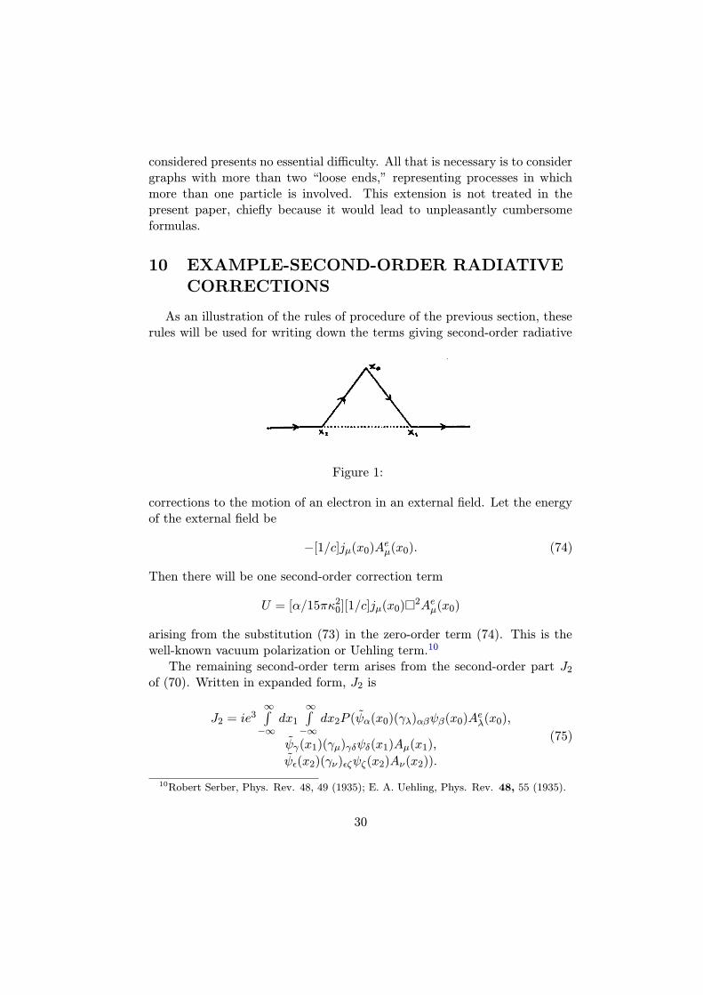
As an illustration of the rules of procedure of the previous section, theserules will be used for writing down the terms giving second-order radiative

Figure 1:

corrections to the motion of an electron in an external field. Let the energyof the external field be

−[1/c]jµ(x0)Aeµ(x0). (74)

Then there will be one second-order correction term

U = [α/15πκ20][1/c]jµ(x0)2Aeµ(x0)

arising from the substitution (73) in the zero-order term (74). This is thewell-known vacuum polarization or Uehling term.10

The remaining second-order term arises from the second-order part J2

of (70). Written in expanded form, J2 is

J2 = ie3∞∫−∞

dx1

∞∫−∞

dx2P (ψα(x0)(γλ)αβψβ(x0)Aeλ(x0),

ψγ(x1)(γµ)γδψδ(x1)Aµ(x1),

ψε(x2)(γν)εζψζ(x2)Aν(x2)).

(75)

10Robert Serber, Phys. Rev. 48, 49 (1935); E. A. Uehling, Phys. Rev. 48, 55 (1935).

30

Next, all admissable graphs with the three vertices x0, x1, x2 are to be drawn.It is easy to see that there are only two such graphs, that G shown in Fig.1, and the identical graph with x1 and x2 interchanged. The full linesare electron lines, the dotted line a photon line. The contribution K(G)is obtained from J2 by substituting according to the rules of Section IX;in this case l = 0, and the primes can be omitted from (71), (72), (73)since only second-order terms are required. The integrand in K(G) canbe reassembled into the form of a matrix product, suppressing the suffixesα, . . . , ζ. Then, multiplying by a factor 2 to allow for the second graph, thecomplete second-order correction to (74) arising from J2 becomes

L = −i[e3/8hc]∞∫−∞

dx1

∞∫−∞

dx2DF (x1 − x2)Aeµ(x0)

×ψ(x1)γνSF (x0 − x1)γµSF (x2 − x0)γνψ(x2).

(76)

This is the term which gives rise to the main part of the Lamb-Retherfordline shift,11 the anomalous magnetic moment of the electron,12 and theanomalous hyperfine splitting of the ground state of hydrogen.13

The above expression L is formally simpler than the corresponding ex-pression obtained by Schwinger, but the two are easily seen to be equivalent.In particular, the above expression does not lead to any great reduction inthe labor involved in a numerical calculation of the Lamb shift. Its advan-tage lies rather in the ease with which it can be written down.

In conclusion, the author would like to express his thanks to the Com-monwealth Fund of New York for financial support, and to Professors Schwingerand Feynman for the stimulating lectures in which they presented their re-spective theories.

Notes added in proof (To Section II). The argument of Section II is an over-simplification of the method of Tomonaga,14 and is unsound. There is an error inthe derivation of (3); derivatives occurring in H(r) give rise to non-commutativitybetween H(r) and field quantities at r′ when r′ is a point on r infinitesimally distantfrom r′. The argument should be amended as follows. Φ is defined only for flatsurfaces t(r) = t, and for such surfaces (3) and (6) are correct. Ψ is defined forgeneral surfaces by (12) and (10), and is verified to satisfy (9). For a flat surface, Φand Ψ are then shown to be related by (7). Finally, since H1 does not involve thederivatives in H, the argument leading to (3) can be correctly applied to prove that

11W.E. Lamb and R.C. Retherford, Phys. Rev. 72, 241 (1947).12P. Kusch and H.M. Foley, Phys. Rev. 74, 250 (1948).13J.E. Nafe and E.B. Nelson, Phys. Rev. 73, 718 (1948); Aage Bohr, Phys. Rev. 73,

1109 (1948).14P. Kusch and H. M. Foley, Phys. Rev. 74, 250 (1948). J. E. Nafe and E. B. Nelson,

Phys. Rev. 73, 718 (1948); Aage Bohr, Phys. Rev. 73, 1109 (1948).

31

for general σ the state-vector Ψ(σ) will completely describe results of observationsof the system on σ.

(To Section III). A covariant perturbation theory similar to that of Section IIIhas previously been developed by E. C. G. Stueckelberg, Ann. d. Phys. 21, 367(1934); Nature, 153, 143 (1944).

(To Section V). Schwinger’s “effective potential” is not HT given by (25), butis H ′T = QHTQ

−1. Here Q is a “square-root” of S(∞) obtained by expand-ing (S(∞))1/2 by the binomial theorem. The physical meaning of this is thatSchwinger specifies states neither by Ω nor by Ω′, but by an intermediate state-vector Ω′′ = QΩ = Q−1Ω′, whose definition is symmetrical between past and future.H ′T is also symmetrical between past and future. For one-particle states, HT andH ′T are identical.

Equation (32) can most simply be obtained directly from the product expansionof S(∞).

(To Section VII). Equation (62) is incorrect. The function S′F is well-behaved,but its fourier transform has a logarithmic dependence on frequency, which makesan expansion precisely of the form (62) impossible.

(To Section X). The term L still contains two divergent parts. One is an “infra-

red catastrophe” removable by standard methods. The other is an “ultraviolet”

divergence, and has to be interpreted as an additional charge-renormalization, or,

better, cancelled by part of the charge-renormalization calculated in Section VIII.

32