the radiation environment for the next generation … radiation environment for the next generation...

The Radiation Environmentfor theNext GenerationSpace Telescope

<Document Control Number>

Janet L. Barth

NASA/Goddard Space Flight CenterGreenbelt, Maryland

John C. Isaacs

Space Telescope Science InstituteBaltimore, Maryland

Christian Poivey

SGT-Inc.Greenbelt, Maryland

September 2000

G S F C

2

Table of Contents

I. INTRODUCTION ................................................................................................................................ 3

II. RADIATION ENVIRONMENT ......................................................................................................... 3

III. DESCRIPTION OF RADIATION EFFECTS ............................................................................... 3

IV. THE NGST MISSION...................................................................................................................... 4

V. TOTAL DOSE AND DEGRADATION.............................................................................................. 5

A. DEGRADATION ENVIRONMENT............................................................................................................ 61. The Plasma Environment................................................................................................................ 62. High Energy Particles – Spacecraft Incident Fluences ................................................................ 123. High Energy Particles – Shielded Fluences ................................................................................. 15

B. TOTAL DOSE ESTIMATES................................................................................................................... 181. Top Level Ionizing Dose Requirement.......................................................................................... 182. Dose at Specific Spacecraft Locations.......................................................................................... 20

C. DISPLACEMENT DAMAGE ESTIMATES ............................................................................................... 20

VI. SINGLE EVENT EFFECTS ANALYSIS..................................................................................... 21

A. HEAVY ION INDUCED SINGLE EVENT EFFECTS.................................................................................. 211. Galactic Cosmic Rays................................................................................................................... 212. Solar Heavy Ions........................................................................................................................... 22

B. PROTON INDUCED SINGLE EVENT EFFECTS ....................................................................................... 221. Trapped Protons ........................................................................................................................... 232. Solar Protons................................................................................................................................ 23

VII. INSTRUMENT INTERFERENCE............................................................................................... 23

VIII. SPACECRAFT CHARGING AND DISCHARGING................................................................. 28

IX. SUMMARY..................................................................................................................................... 28

X. REFERENCES ................................................................................................................................... 29

APPENDICES........................................................................................................................................... A-1

3

I. Introduction

The purpose of this document is to define the radiation environment for the evaluation of degradation dueto total ionizing and non-ionizing dose and of single event effects (SEEs) for the Next Generation SpaceTelescope (NGST) instruments and spacecraft. The analysis took into account the radiation exposure forthe nominal five-year mission at the Earth-Sun L2 Point and assumes a launch date in June 2009. Thetransfer trajectory out to the L2 position has not yet been defined, therefore, this evaluation does notinclude the impact of passing through the Van Allen belts. Generally, transfer trajectories do not contributeto degradation effects; however, single event effects and deep dielectric charging effects must be taken intoconsideration especially if critical maneuvers are planned during the Van Allen belt passes.

II. Radiation Environment

The natural space radiation environment of concern for damage to spacecraft electronics is classified intotwo populations, 1) the transient particles which include protons and heavier ions of all of the elements ofthe periodic table, and 2) the trapped particles which include protons, electrons and heavier ions. Thetrapped electrons have energies up to 10 MeV and the trapped protons and heavier ions have energies up to100s of MeV. The transient radiation consists of galactic cosmic ray particles and particles from solarevents (coronal mass ejections and flares). The cosmic rays have low level fluxes with energies up to TeV.The solar eruptions periodically produce energetic protons, alpha particles, heavy ions, and electrons. Thesolar protons have energies up to 100’s MeV and the heavier ions reach the GeV range. All particles areisotropic and omnidirectional to the first order.

Space also contains low energy plasma of electrons and protons with fluxes up to 1012 cm2/sec. Theplasmasphere environment and the low energy (< 0.1 MeV) component of the charged particles are aconcern in the near-earth environment. In the outer regions of the magnetosphere and in interplanetaryspace, the plasma is associated with the solar wind. Because of its low energy, thin layers of materialeasily stop the plasma so it is not a hazard to most spacecraft electronics. However, it is damaging tosurface materials and differentials in the plasma environment can contribute to spacecraft surface chargingand discharging problems [1,2].

III. Description of Radiation Effects

Radiation effects that are important to consider for instrument and spacecraft design fall roughly into threecategories: degradation from total ionizing dose (TID), degradation from non-ionizing energy loss (NIEL),and single event effects. Total ionizing dose in electronics is a cumulative long term ionizing damage dueto protons and electrons. It causes threshold shifts, leakage current and timing skews. The effect firstappears as parametric degradation of the device and ultimately results in functional failure. It is possible toreduce TID with shielding material that absorbs most electrons and lower energy protons. As shielding isincreased, shielding effectiveness decreases because of the difficulty in slowing down the higher energyprotons. When a manufacturer advertises a part as “rad-hard”, he is almost always referring to its totalionizing dose characteristics. Rad-hard does not usually imply that the part is hard to non-ionizing dose orsingle event effects.

4

Displacement damage is cumulative long-term non-ionizing damage due to protons, electrons, andneutrons. The particles produce defects in optical materials that result in charge transfer degradation. Itaffects the performance of optocouplers (often a component in power devices), solar cells, CCDs, andlinear bipolar devices. The effectiveness of shielding depends on the location of the device. For example,coverglasses over solar cells reduce electron damage and proton damage by absorbing the low energyparticles. Increasing shielding, however, is not usually effective for optoelectronic components because thehigh-energy protons penetrate the most feasible spacecraft electronic enclosures. For detectors ininstruments it is necessary to understand the instrument geometry to determine the vulnerability to theenvironment.

Single event effects are caused through ionization by a single charged particle as it passes through asensitive junction of an electronic device. They are caused by heavier ions, but for some devices, protonscan induce single event effects. In some cases SEEs are induced through direct ionization by the proton,but in most instances, proton induced effects are the result of secondary particles that are produced whenthe proton collides with a nucleus of the material in the device. Some single event effects are non-destructive as in the case of single event upsets (SEUs), single event transients (SETs), multiple bit errors(MBEs), single event hard errors (SHEs), etc. Single event effects can also be destructive as in the case ofsingle event latchups (SELs), single event gate ruptures (SEGRs), and single event burnouts (SEBs). Theseverity of the effect can range from noisy data to loss of the mission, depending on the type of effect andthe criticality of the system in which it occurs. Shielding is not an effective mitigator for single eventeffects because they are induced by very penetrating high energy particles. The preferred method fordealing with destructive failures is to use SEE-hard parts. When SEE-hard parts are not available, latchupprotection circuitry is sometimes used in conjunction with failure mode analysis. For non-destructiveeffects, mitigation takes the form of error-detection and correction codes (EDACs), filtering circuitry, etc.

Total ionizing dose is primarily caused by protons and electrons trapped in the Van Allen belts and solarevent protons. As electrons are slowed down, their interactions with orbital electrons of the shieldingmaterial produce a secondary photon radiation known as bremsstrahlung. Generally, the dose due togalactic cosmic ray ions and proton secondaries is negligible in the presence of the other sources. Forsurface degradation, it is also important to include the effects of very low energy particles.

Single event effects can be induced by heavy ions (solar events and galactic cosmic rays) and, in somedevices, protons (trapped and solar events) and neutrons. Displacement damage is primarily due to trappedand solar protons and also neutrons that are produced by interactions of primary particles with theatmosphere and spacecraft materials.∗ Spacecraft charging can occur on the surface of the spacecraft due tolow energy electrons. Deep dielectric charging occurs when high energy electrons penetrate the spacecraftand collect in dielectric materials.

IV. The NGST Mission

The NGST spacecraft will be transferred out to the L2 point via a trajectory that has not yet been defined.While in the transfer, NGST will pass through the trapped proton and electron belts. These exposurescould constitute a single event effect risk during some maneuvers but will not contribute to significantdegradation effects. During the transfer trajectory, NGST will also encounter varying levels of galactic

______________________∗ In avionics applications it is necessary to consider neutrons that are produced by interactions of primary particles withthe atmosphere.

5

cosmic ray heavy ions and possibly protons and heavier ions from solar events. It will also be necessary totake the charging effects of the trapped electrons into account.

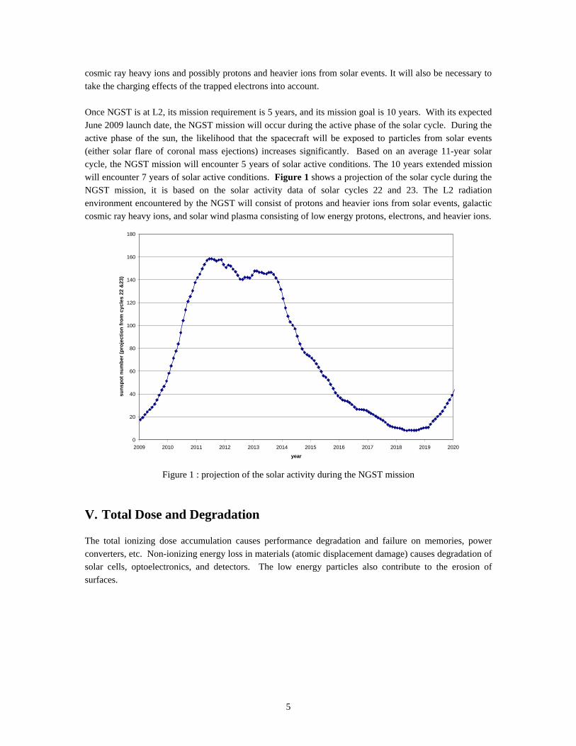
Once NGST is at L2, its mission requirement is 5 years, and its mission goal is 10 years. With its expectedJune 2009 launch date, the NGST mission will occur during the active phase of the solar cycle. During theactive phase of the sun, the likelihood that the spacecraft will be exposed to particles from solar events(either solar flare of coronal mass ejections) increases significantly. Based on an average 11-year solarcycle, the NGST mission will encounter 5 years of solar active conditions. The 10 years extended missionwill encounter 7 years of solar active conditions. Figure 1 shows a projection of the solar cycle during theNGST mission, it is based on the solar activity data of solar cycles 22 and 23. The L2 radiationenvironment encountered by the NGST will consist of protons and heavier ions from solar events, galacticcosmic ray heavy ions, and solar wind plasma consisting of low energy protons, electrons, and heavier ions.

0

20

40

60

80

100

120

140

160

180

2009 2010 2011 2012 2013 2014 2015 2016 2017 2018 2019 2020

year

sun

spo

t n

um

ber

(p

roje

ctio

n f

rom

cyc

les

22 &

23)

Figure 1 : projection of the solar activity during the NGST mission

V. Total Dose and Degradation

The total ionizing dose accumulation causes performance degradation and failure on memories, powerconverters, etc. Non-ionizing energy loss in materials (atomic displacement damage) causes degradation ofsolar cells, optoelectronics, and detectors. The low energy particles also contribute to the erosion ofsurfaces.

6

A. Degradation Environment

At L2 low energy particles from the solar wind plasma contribute to the degradation of surface materials.The higher energy particles trapped in the Van Allen belts and from high energy solar events can penetratesolar cell coverglasses and solar array substrate structures and, therefore, are responsible for solar celldegradation.

1. The Plasma Environment

The solar wind is composed of protons and heavier ions (roughly 95% and H+ and 5% H++ ) combined withenough electrons to form an electrically neutral plasma. It is commonly described in terms of averagedensity, velocity, and temperature. Table 1 lists average values or a range of values for these parameters

Table 1Average Solar Wind Parameters

Density 1-10 particles/cm3

Velocity 400 km/sEnergy “a few eV”

A model of the solar wind plasma that can be used for engineering applications such as materialdegradation analysis and spacecraft surface charging is not available at this time. However, a joint effort atGSFC and MFSC is underway to develop a plasma model for these applications. In the meantime, recentsatellite measurements provide a good understanding of the dynamic range of the density, velocity, andenergy temperature.

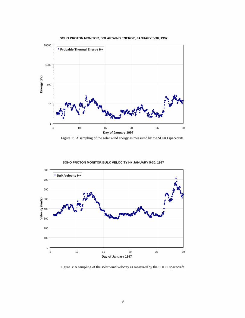
The plasma environment for the NGST spacecraft will depend on its position relative to the magnetotailregion of the earth’s magnetosphere.* The data given here from the GEOTAIL and SOHO spacecraft give asampling of the expected range of the solar wind parameters inside and outside of the magnetotail. TheSOHO spacecraft has also measured plasma parameters with the Mass Time-of-Flight/Proton Monitor.Measurements [3] are given here outside of the tail region at ~230 earth radii during January 1997.Figures 2-4 plot the plasma density, velocity, and energy. A sampling of the data is given in Table 2. Thedata in the table and figures show that the average solar wind parameters given in Table 1 comparefavorably with the SOHO measurements.

______________________* The magnetotail of the magnetosphere is formed by the interactions of the solar wind with the Earth’s magnetic field.In the solar direction, the magnetic field lines are compressed down to ~12 earth radii under average solar-magneticconditions. In the anti-solar direction, the solar wind “stretches” the magnetic field lines out to hundreds of earth radii,forming the magnetotail.

7

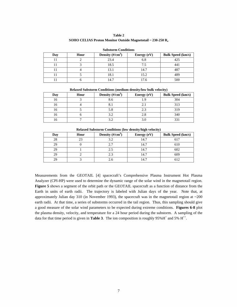
Table 2SOHO CELIAS Proton Monitor Outside Magnetotail ~ 230-250 Re

Substorm ConditionsDay Hour Density (#/cm3) Energy (eV) Bulk Speed (km/s)11 2 23.4 6.8 42511 3 18.5 7.5 44111 4 13.1 14.7 48711 5 18.1 15.2 48911 6 14.7 17.6 500

Relaxed Substorm Conditions (medium density/low bulk velocity)Day Hour Density (#/cm3) Energy (eV) Bulk Speed (km/s)16 3 8.6 1.9 30416 4 8.1 2.1 31316 5 5.8 2.3 31916 6 3.2 2.8 34016 7 3.2 3.0 331

Relaxed Substorm Conditions (low density/high velocity)Day Hour Density (#/cm3) Energy (eV) Bulk Speed (km/s)28 23 3.2 14.7 61729 0 2.7 14.7 61029 1 2.5 14.7 60229 2 2.3 14.7 60929 3 2.6 14.7 612

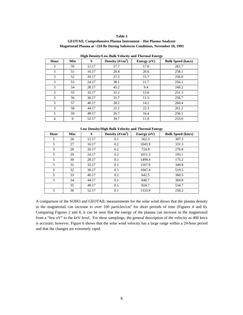
Measurements from the GEOTAIL [4] spacecraft’s Comprehensive Plasma Instrument Hot PlasmaAnalyzer (CPI-HP) were used to determine the dynamic range of the solar wind in the magnetotail region.Figure 5 shows a segment of the orbit path or the GEOTAIL spacecraft as a function of distance from theEarth in units of earth radii. The trajectory is labeled with Julian days of the year. Note that, atapproximately Julian day 310 (in November 1993), the spacecraft was in the magnetotail region at ~200earth radii. At that time, a series of substorms occurred in the tail region. Thus, this sampling should givea good measure of the solar wind parameters to be expected during extreme conditions. Figures 6-8 plotthe plasma density, velocity, and temperature for a 24 hour period during the substorm. A sampling of thedata for that time period is given in Table 3. The ion composition is roughly 95%H+ and 5% H++.

8

Table 3GEOTAIL Comprehensive Plasma Instrument – Hot Plasma Analyzer

Magnetotail Plasma at ~210 Re During Substorm Conditions, November 18, 1993

High Density/Low Bulk Velocity and Thermal EnergyHour Min S Density (#/cm3) Energy (eV) Bulk Speed (km/s)

3 50 12.17 27.7 17.8 261.73 51 16.17 28.4 20.6 258.13 52 20.17 27.5 15.7 256.03 53 24.17 38.1 11.7 256.13 54 28.17 45.2 9.4 249.23 55 32.17 31.2 13.6 251.33 56 36.17 31.7 11.5 256.73 57 40.17 28.2 14.2 260.43 58 44.17 21.1 22.3 261.23 59 48.17 26.7 16.4 256.14 0 52.17 39.7 11.0 253.0

Low Density/High Bulk Velocity and Thermal EnergyHour Min S Density (#/cm3) Energy (eV) Bulk Speed (km/s)

5 26 12.17 0.1 562.3 307.35 27 16.17 0.2 1043.9 331.35 28 20.17 0.2 724.9 276.85 29 24.17 0.2 1011.3 193.15 30 28.17 0.1 1499.4 175.25 31 32.17 0.1 1167.0 349.85 32 36.17 0.1 1047.4 519.55 33 40.17 0.2 642.5 360.55 34 44.17 0.1 848.7 369.8

35 48.17 0.1 824.7 534.75 36 52.17 0.1 1333.9 258.2

A comparison of the SOHO and GEOTAIL measurements for the solar wind shows that the plasma densityin the magnetotail can increase to over 100 particles/cm3 for short periods of time (Figures 4 and 6).Comparing Figures 2 and 8, it can be seen that the energy of the plasma can increase in the magnetotailfrom a “few eV” to the keV level. For these samplings, the general description of the velocity as 400 km/sis accurate; however, Figure 6 shows that the solar wind velocity has a large range within a 24-hour periodand that the changes are extremely rapid.

9

Figure 2: A sampling of the solar wind energy as measured by the SOHO spacecraft.

Figure 3: A sampling of the solar wind velocity as measured by the SOHO spacecraft.

SOHO PROTON MONITOR, SOLAR WIND ENERGY, JANUARY 5-30, 1997

1

10

100

1000

10000

5 10 15 20 25 30

Day of January 1997

En

erg

y (e

V)

Probable Thermal Energy H+

SOHO PROTON MONITOR BULK VELOCITY H+ JANUARY 5-30, 1997

0

100

200

300

400

500

600

700

800

5 10 15 20 25 30

Day of January 1997

Vel

oci

ty (

km/s

)

Bulk Velocity H+

10

Figure 4: A sampling of the solar wind density as measured by the SOHO spacecraft.

Figure 5: Position of GEOTAIL in the magnetotail.

SOHO PROTON MONITOR, H+ DENSITY, JANUARY 5-30, 1997

0.01

0.1

1

10

100

1000

5 10 15 20 25 30

Day of January 1997

Den

sity

(p

arti

cles

/cm

3 )H+ Density

11

Figure 6: A sampling of the ion density as sampled by GEOTAIL.

Figure 7: A sampling of ion bulk velocity by GEOTAIL.

GEOTAIL CPI-HP, Ion Density (Particles/cc), November 18, 1993

0.01

0.1

1

10

100

1000

0 1 2 3 4 5 6 7 8 9 10 11 12 13 14 15 16 17 18 19 20 21 22 23 24

UT (Hour)

Den

sity

(p

arti

cles

/cm

3 )

Ion Density

GEOTAIL CPI-HP, Ion Bulk Velocity (km/s), November 18, 1993

0

100

200

300

400

500

600

700

800

0 1 2 3 4 5 6 7 8 9 10 11 12 13 14 15 16 17 18 19 20 21 22 23 24

UT (Hour)

Vel

oci

ty (

km/s

)

12

Figure 8: A sampling of ion energy by GEOTAIL.

2. High Energy Particles – Spacecraft Incident Fluences

The spacecraft incident proton fluence levels given in this document are most often used for standard solarcell analyses that take into account the coverglass thickness of the cell. There are three possible sources ofhigh energy particles: trapped protons and trapped electrons encountered in the transfer trajectory andprotons from solar events that can occur anytime during the five to seven solar active years of the mission.The trapped particles encountered in the transfer trajectory cannot be evaluated at this time but are usuallynot a factor in degradation analyses. The proton fluence levels are also used to determine displacementdamage effects, however, most analysis methods require that the surface incident particles be transportedthrough the materials surrounding the sensitive components. The proton fluences behind nominalaluminum shield thicknesses are given in Section V.A.3.

When the transfer trajectory is known, the trapped particle fluxes will be estimated with NASA’s AP-8 [5]model for protons and AE-8 [6] model for electrons. The models come in solar minimum and maximumversions. The uncertainty factors defined for the models are a factor of 2 for the AP-8 and 2 to 5 for theAE-8. These uncertainty factors apply to long term averages expected over a 6 month mission duration.Daily values can fluctuate by two to three orders of magnitude depending on the level of activity on the sunand within the magnetosphere.

The solar proton levels can now be estimated from the new Emission of Solar Proton (ESP) model [7].Previously, estimates of solar proton levels were obtained from models [8,9] that were largely empirical innature, making it difficult to add data to the model from more recent solar cycles. The ESP model is basedon satellite data from solar cycles 20, 21, and 22. The distribution of the fluences for the events is obtainedfrom maximum entropy theory, and design limits in the worst case models are obtained from extreme valuetheory.

GEOTAIL CPI-HP, Ion Energy at 210 Earth Radii in Magnetotail, Nov. 18, 1993

1

10

100

1000

10000

0 1 2 3 4 5 6 7 8 9 10 11 12 13 14 15 16 17 18 19 20 21 22 23 24UT (Hour)

En

erg

y (e

V)

Ion (95% H+, 5% He++)

13

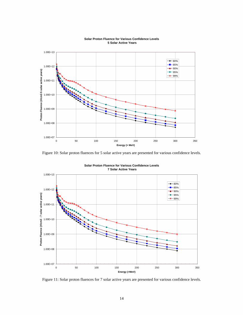
Total integral solar proton fluences were estimated for 1, 5, and 7 solar active years with 5 years being thenumber of years to consider for the nominal mission and 7 years the number of years to consider for the 10years extended mission. Tables A1-A3 give the fluence levels as a function of particle energy for 80, 85,90, 95, and 99% confidence levels. Figures 9-11 are plots of the energy-fluences spectra for 1, 5, and 7solar active years for the given confidence levels. In addition, Figure 12 compares the 1, 5, and 7 yearsolar proton fluence levels for the 95% confidence level. The energies are in units of >MeV and thefluences are in units of particles/cm2. These values do not include a design margin. The solar protonpredictions are not linear over time; therefore, these estimates may be invalid if extrapolated for longermission durations.

Solar Proton Fluence for Various Confidence Levels 1 Solar Active Year

1.00E+06

1.00E+07

1.00E+08

1.00E+09

1.00E+10

1.00E+11

1.00E+12

0 50 100 150 200 250 300 350

Energy (> MeV)

Pro

ton

Flu

ence

(#/

cm2-

1 s

ola

r ac

tive

yea

r)

80%85%90%95%99%

Figure 9: Solar proton fluences for 1 solar active year are presented for various confidence levels.

14

Solar Proton Fluence for Various Confidence Levels 5 Solar Active Years

1.00E+07

1.00E+08

1.00E+09

1.00E+10

1.00E+11

1.00E+12

1.00E+13

0 50 100 150 200 250 300 350

Energy (> MeV)

Pro

ton

Flu

ence

(#/

cm2-

5 so

lar

acti

ve y

ears

)

80%85%90%95%99%

Figure 10: Solar proton fluences for 5 solar active years are presented for various confidence levels.

Solar Proton Fluence for Various Confidence Levels 7 Solar Active Years

1.00E+07

1.00E+08

1.00E+09

1.00E+10

1.00E+11

1.00E+12

1.00E+13

0 50 100 150 200 250 300 350

Energy (>MeV)

Pro

ton

Flu

ence

(#/

cm2

- 7

sola

r ac

tive

yea

rs)

80%85%90%95%99%

Figure 11: Solar proton fluences for 7 solar active years are presented for various confidence levels.

15

Solar Proton Fluence for 1,5 and 7 Solar Active years 95% Confidence Level

1.00E+07

1.00E+08

1.00E+09

1.00E+10

1.00E+11

1.00E+12

1.00E+13

0 50 100 150 200 250 300 350

Energy (> MeV)

Pro

ton

Flu

ence

(#/

cm2)

5 Solar Active Years7 Solar Active Years1 Solar Active Year

Figure 12: Solar proton fluences for a 95% confidence level are presented for 1, 5, and 7 solar active years.

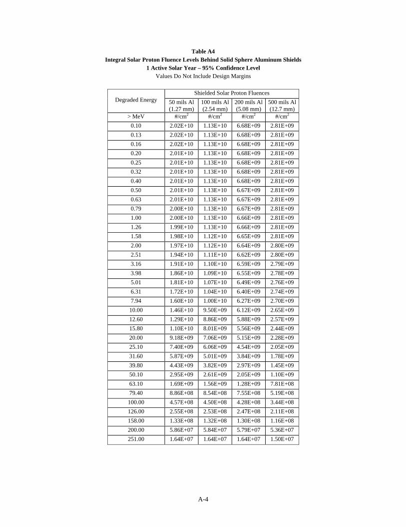
3. High Energy Particles – Shielded Fluences

Evaluation of non-ionizing energy loss damage requires the use of shielded fluence levels. For this analysisnominal shielding thicknesses of 50, 100, 200, and 500 mils of aluminum were used for a generic solidsphere geometry. The spacecraft incident, solar proton estimates for the 95% confidence level and for 1, 5,and 7 year solar active years were transported through the shield thickness to obtain fluence estimatesbehind the shielding. Tables A4-A6 give the degraded energy spectra. The spectra are plotted inFigures 13-15. Figure 16 shows a comparison for 1, 5, and 7 solar active years for 100 mil shielding case.It can be seen from the figures that even though low energy particles are absorbed by the shielding, the lowenergy range of the spectrum is filled in by the higher energy protons as they are degraded by passingthrough the material.

16

Shielded integral Solar Proton Fluence for 1 Solar Active Year 95% Confidence Level - Values do not include Design Margins

1.00E+07

1.00E+08

1.00E+09

1.00E+10

1.00E+11

1.00E+12

0.1 1 10 100 1000

Energy (> MeV)

Pro

ton

s (#

/cm

2- 1

So

lar

Act

ive

Yea

r)

Spacecraft incident50 mils Al (1.27 mm)100 mils Al (2.54 mm)200 mils Al (5.08 mm)500 mils Al (12.7 mm)

Figure 13: Shielded solar proton energy spectra for 1 solar active year, 95% confidence level.

Shielded integral Solar Proton Fluences for 5 Solar Active Years 95% Confidence Level - Values do not include Design Margins

1.00E+07

1.00E+08

1.00E+09

1.00E+10

1.00E+11

1.00E+12

1.00E+13

0.1 1 10 100 1000

Energy (>MeV)

Pro

ton

s(#/

cm2-

5 S

ola

r A

ctiv

e ye

ars)

Spacecraft Incident50 mils Al (1.27 mm)100 mils Al (2.54 mm)200 mils Al (5.08 mm)500 mils Al (12.7 mm)

Figure 14: Shielded solar proton energy spectra for 5 solar active years, 95% confidence level.

17

Shielded Integral Solar Proton Fluences for 7 Solar Active years 95% Confidence Level - Values do not include Design Margins

1.00E+07

1.00E+08

1.00E+09

1.00E+10

1.00E+11

1.00E+12

1.00E+13

0.1 1 10 100 1000

Energy (> MeV)

Pro

ton

s (#

/cm

2 -

7 so

lar

acti

ve y

ears

)

Spacecraft incident50 mils Al (1.27 mm)100 mils Al (2.54 mm)200 mils Al (5.08 mm)500 mils Al (12.7 mm)

Figure 15: Shielded solar proton energy spectra for 7 solar active years, 95% confidence level.

Shielded Integral Solar Proton Fluences for 100 mils (2.54mm) Aluminum 95% Confidence Level - Value do not include Design Margins

1.00E+07

1.00E+08

1.00E+09

1.00E+10

1.00E+11

0.1 1.0 10.0 100.0 1000.0

Energy (> MeV)

Pro

ton

s (#

/cm

2)

1 Solar Active Year5 Solar Active Years7 Solar Active Years

Figure 16: Shielded solar proton energy spectra for 100 mils aluminum 95% confidence level

18

B. Total Dose Estimates

1. Top Level Ionizing Dose Requirement

Doses are calculated from the surface incident integral fluences as a function of aluminum shield thicknessfor a simple geometry. The geometry model used for spacecraft applications is the solid sphere. The solidsphere doses represent an upper boundary for the dose inside an actual spacecraft and are used as a top-level requirement. In cases where the amount of shielding surrounding a sensitive location is difficult toestimate, a more detailed analysis of the geometry of the spacecraft structure may be necessary to evaluatethe expected dose levels. This is done by modeling the electronic boxes or instruments and the spacecraftstructure. The amount of shielding surrounding selected sensitive locations is estimated using solid anglesectoring and 3-dimensional ray tracing. Doses obtained by sectoring methods must be verified for 5-10%of the sensitive locations with full Monte Carlo simulations of particle trajectories through the structure formany histories.

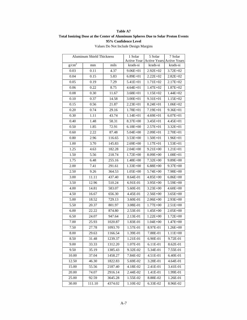
Table A7 and Figures 17 and 18 give the top-level total ionizing dose requirement for the 5 year NGSTmission and for the 10 year extended mission. The doses are given for 1, 5, and 7 solar active years for a95% confidence level. The best estimate at this time predicts 5 solar active years for the nominal missionand 7 solar active years for the extended mission given the 2009 NGST launch. The doses are calculatedhere as a function of aluminum shield thickness in units of krads in silicon. For the nominal 100 mils ofequivalent aluminum shielding and the 5 years nominal mission , the dose requirement is 18 krad-Si withno design margin. For the nominal 100 mils of equivalent aluminum shielding and the 10 years extendedmission , the dose requirement is 24 krad-Si with no design margin A minimum design margin of x 2 isrecommended.

19

Total Dose at the Center of Solid Aluminum Spheres- Top Level Requirement 95% Confidence Level - Values do not include Design Margin

0.01

0.10

1.00

10.00

100.00

1000.00

0 500 1000 1500 2000 2500 3000 3500 4000 4500 5000

Aluminum Shield Thickness (mils)

Do

se (

krad

-Si)

1 Solar Active Year5 Solar Active Years7 Solar Active years

Figure 17: Total ionizing dose from solar proton events for 1, 5, and 7 solar active years is presented.

Total Dose at the Center of Solid Aluminum Spheres- Top Level Requirement 95% Confidence Level - Values do not include Design Margin

0.01

0.10

1.00

10.00

100.00

1000.00

0 100 200 300 400 500 600 700 800 900 1000

Aluminum Shield Thickness (mils)

Do

se (

krad

-Si)

1 Solar Active Year

5 Solar Active Years

7 Solar Active years

Figure 18: Total ionizing dose from solar proton events for 1, 5, and 7 solar active years is presented.

20

2. Dose at Specific Spacecraft Locations

In cases where parts cannot meet the top level design requirement and a “harder” part cannot be substituted,it is often beneficial to employ more accurate methods of determining the dose exposure for somespacecraft components to qualify the parts. One such method for calculating total dose, solid anglesectoring/3-dimensional ray tracing, is accomplished in three steps:

1) Model the spacecraft structure: -develop a 3-D model of the spacecraft structures and components -develop a material library -define sensitive locations2) Model the radiation environment: -define the spacecraft incident radiation environment -develop a particle attenuation model using theoretical shielding configurations (similar to dose-depth curves).3) Obtain results for each sensitive location: -divide the structural model into solid angle sectors -ray trace through the sectors to calculate the material mass distribution

-use the ray trace results to calculate total doses from the particle attenuation model.

Once the basic structural model has been defined, total doses can be obtained for any location in thespacecraft in a short time (in comparison to Monte Carlo methods). The value of dose mitigation measurescan be accurately evaluated be adding the changes to the model and recalculating the total dose. Forspacecraft with strict weight budgets, the 3-D ray trace method, the total dose design requirement can bedefined at a box or instrument level avoiding unnecessary use of expensive or increasingly unavailableradiation hardened parts.

As the design of the NGST evolves, it may become necessary to estimate the doses at specific locations inthe spacecraft or instruments. Often the dose requirement can be met by modeling the surroundingelectronic box only or by modeling only the instrument.

C. Displacement Damage Estimates

Total non-ionizing energy loss damage is evaluated by combining the shielded proton energy spectra givenSection V.A.3 with the NIEL Non Ionizing Energy Loss (NIEL) response curves for the material and theresults of laboratory radiation of the devices sensitive to atomic displacement damage. The level of thehazard is highly dependent on the device type and can be process specific. For the NGST mission, it isimportant to keep in mind that some optoelectronic devices experience enough damage during one largesolar proton event to cause the device to fail. It is necessary that the parts list screening for radiation alsoinclude a check for devices that are susceptible to displacement damage.

21

VI. Single Event Effects Analysis

A. Heavy Ion Induced Single Event Effects

Some electronic devices are susceptible to single event effects (SEEs), e.g., single event upsets, singleevent latch-up, single event burn-out. Because of their ability to penetrate to the sensitive regions ofdevices and their ability to ionize materials, heavy ions cause SEEs by the direct deposit of charge. Thequantity most frequently used to measure an ion’s ability to deposit charge in devices is linear energytransfer (LET). Heavy ion abundances are converted to total LET spectra. Once specific parts are selectedfor the mission and, if necessary, characterized by laboratory testing, the LET spectra for the heavy ions areintegrated with the device characterization to calculate SEE rates. Heavy ion populations that havesufficient numbers to be a SEE hazard are the galactic cosmic rays and those from solar events.

1. Galactic Cosmic Rays

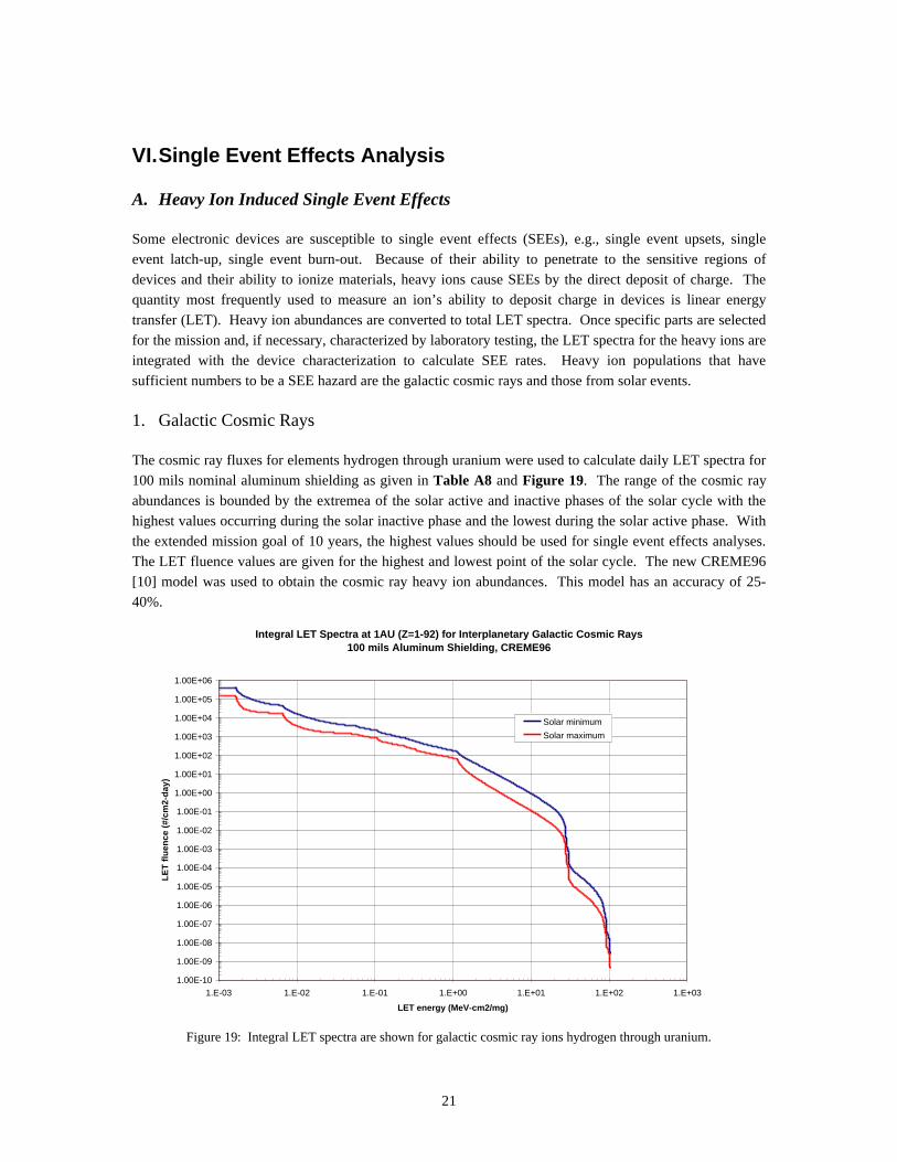
The cosmic ray fluxes for elements hydrogen through uranium were used to calculate daily LET spectra for100 mils nominal aluminum shielding as given in Table A8 and Figure 19. The range of the cosmic rayabundances is bounded by the extremea of the solar active and inactive phases of the solar cycle with thehighest values occurring during the solar inactive phase and the lowest during the solar active phase. Withthe extended mission goal of 10 years, the highest values should be used for single event effects analyses.The LET fluence values are given for the highest and lowest point of the solar cycle. The new CREME96[10] model was used to obtain the cosmic ray heavy ion abundances. This model has an accuracy of 25-40%.

Integral LET Spectra at 1AU (Z=1-92) for Interplanetary Galactic Cosmic Rays 100 mils Aluminum Shielding, CREME96

1.00E-10

1.00E-09

1.00E-08

1.00E-07

1.00E-06

1.00E-05

1.00E-04

1.00E-03

1.00E-02

1.00E-01

1.00E+00

1.00E+01

1.00E+02

1.00E+03

1.00E+04

1.00E+05

1.00E+06

1.E-03 1.E-02 1.E-01 1.E+00 1.E+01 1.E+02 1.E+03

LET energy (MeV-cm2/mg)

LE

T f

luen

ce (

#/cm

2-d

ay)

Solar minimum

Solar maximum

Figure 19: Integral LET spectra are shown for galactic cosmic ray ions hydrogen through uranium.

22

2. Solar Heavy Ions

The heavy ions from solar flares and coronal mass ejections can also produce single event effects. Thesolar event fluxes for the elements hydrogen through uranium were used to calculate daily LET spectra for100 mils nominal aluminum shielding in units of average LET flux per second. The intensity of the fluxesvaries over the duration of an event; therefore, values are averaged over the worst week of the solar cycle,the worst day of the solar cycle, and the peak of the October 1989 solar event. Table A9 and Figure 20give the solar heavy ion LET predictions for the NGST mission. The new CREME96 model was also usedto calculate the solar heavy ion levels. An uncertainty factor for the solar heavy ion model has not beenreleased.

Integral LET Spectra at 1 AU (Z=1-92) for Interplanetary Solar Particle Events 100 mils Aluminum Shielding, CREME96

1.00E-11

1.00E-10

1.00E-09

1.00E-08

1.00E-07

1.00E-06

1.00E-05

1.00E-04

1.00E-03

1.00E-02

1.00E-01

1.00E+00

1.00E+01

1.00E+02

1.00E+03

1.00E+04

1.00E+05

1.00E+06

1.00E-03 1.00E-02 1.00E-01 1.00E+00 1.00E+01 1.00E+02 1.00E+03

LET Energy (MeV-cm2/mg)

LE

T F

luen

ce (

#/cm

2-s)

Average Over Peak

Average Over Worst Day

Average Over Worst Week

Figure 20: Integral LET spectra are shown for hydrogen through uranium for the October 1989 solar particle event.

B. Proton Induced Single Event Effects

In some devices, single event effects are also induced by protons. Protons from the trapped radiation beltsand from solar events do not generate sufficient ionization (LET < 1 MeV-cm2 /mg) to produce the criticalcharge necessary for SEEs to occur in most electronics. More typically, protons cause Single Event Effectsthrough secondary particles via nuclear interactions, that is, spallation and fractionation products. Becausethe proton energy is important in the production (and not the LET) of the secondary particles that cause theSEEs, device sensitivity to these particles is typically expressed as a function of proton energy rather thanLET.

23

1. Trapped Protons

Trapped protons can be a concern for single event effects during the transfer trajectory passes through thetrapped particle radiation belts. The proton fluxes in the intense regions of the belts reach levels that arehigh enough to induce upsets or latchups. The timing of critical operations during the transfer trajectoryshould be analyzed to determine the trapped proton environment at the time of the operation.

2. Solar Protons

Protons from solar events can also be a single event effects hazard for the NGST spacecraft. Theseenhanced levels of protons could occur anytime during the 5 to 10 year mission but are most likely duringthe portion of the mission that occurs during the active phase of the solar cycle. As with the solar heavyion LET, solar proton fluxes are averaged over worst day, worst week, and the peak of the October 1989solar event. The proton flux averages for a nominal 100 mils of shielding are given in Table A10 and areshown in Figure 21.

1 .0 E-03

1 .0 E-02

1 .0 E-01

1.0E+00

1.0E+01

1.0E+02

1.0E+03

1.0E+04

1.0E+05

1 1 0 1 0 0 1000

E n e r g y ( M e V )

Pa

rtic

les

(#

/cm

2/s

/Me

V)

A v e r a g e O ve r P e a k

A v e r a g e O ve r Wors t Day

A v e r a g e O ve r Wors t W e e k

V a l u e s D o N o t Include Des ign Marg in

D ifferent ial Solar Proton Event Fluxes at 1 AU100 m ils A luminum S hie lding, CREME96

Figure 21: Solar proton fluxes for single event effects evaluation.

VII. Instrument Interference

For NGST the particle background is also a concern for instrument observations. To estimate the nominalparticle background level, the energy spectra for galactic cosmic ray heavy ion elements were estimatedwith the CREME96 model and summed. Fifty mils of aluminum shielding was assumed. The result isshown in Figure 22. Note that the hydrogen component dominates the total number of ions. The total ionflux was integrated over energy to obtain a background count of 5 ions/cm2/s.

24

Total D ifferential Ion Flux - GCR BackgroundShielded - 50 mils Al, CREME96 (Z=1-92)

1.0E-08

1.0E-07

1.0E-06

1.0E-05

1.0E-04

1.0E-03

1.0E-02

0.1 1 10 100 100 0 1000 0 100000

Energy (MeV/n)

Ion

s (

#/c

m2 /s

/Me

V/n

))

Total GCR

H GCR

Integrated Over Energy = 5 ions/cm2/s

Figure 22: Total differential fluence for all galactic cosmic ray particles for a 1 second time period.

Particle interference during solar events is of particular concern because it can impact the observation timesof the instruments. To obtain an estimate for the peak particle count, the total number of particles wasestimated from the solar heavy ion model of the CREME96 code which is based on the October 1989 solarparticle event. The particles were summed and integrated using the same method as with the galacticcosmic ray background. It was estimated the particle rate is approximately 2.5 x 105 ions/cm2/s. Theresults are shown in Figure 23.

Total Differential Ion Flux - Averaged 5-Min Peak during Solar EventShielded - 50 mils Al, CREME96 (Z=1-92)

1 .0E-1 0

1 .0E-0 9

1 .0E-0 8

1 .0E-0 7

1 .0E-0 6

1 .0E-0 5

1 .0E-0 4

1 .0E-0 3

1 .0E-0 2

1 .0E-0 1

1.0E+00

1.0E+01

1.0E+02

1.0E+03

1.0E+04

1.0E+05

0.1 1 1 0 100 1000 10000 100000

Energy (MeV/n)

Ion

s (#

/cm

2/s

/Me

V/n

))

Total Solar Integrated Over Energy = 2.5 x 105 ions/cm2/s

Figure 23: Total differential fluence of all predicted solar particles based on the October 1989 event

25

It is necessary to have a clearer understanding of how the solar particle events impact viewing and datacollection activities on the NGST. Therefore, solar proton flux data were obtained from the SpaceEnvironment Monitor (SEM) Mission of the Geosynchronous Operational Environmental Satellites(GOES) [11]. The 5 minute average data were extracted from the GOES SEM data base* and converted tointegral flux in particles/cm2/s/steradian for proton flux levels greater than 1, 5, 10, 30, 50, 60 and 100MeV, for the years 1986 through 1996. These data were converted to hourly averages in order to reducethe size of the data set.

The distribution of solar proton flux for particles with energies greater than 30 and 50 MeV were firstanalyzed. The distribution is measured by counting the number of hours the average flux was greater than1, 2, 5, 10, 20, or 50 particles/cm2/s for each year, and converting hours to days for presentation purposes.The results are shown in Figures 24 and 25.

020406080

100120140160180200

1986 1987 1988 1989 1990 1991 1992 1993 1994 1995 1996

Cumulative Distribution of Solar Proton Flux > 30MeV

Flux > 1 part/cm^2/secFlux > 2 part/cm^2/secFlux > 5 part/cm^2/sec


Day

s of

Yea

r

Year

Figure 24: The cumulative distribution of > 30 MeV solar protons for the last solar cycle.

0

20

40

60

80

100

120

140

160

1986 1987 1988 1989 1990 1991 1992 1993 1994 1995 1996

Cumulative Distribution of Solar Proton Flux > 50MeV



Day

s of

Yea

r

Year

Figure 25: The cumulative distribution of > 50 MeV solar protons for the last solar cycle______________________* The authors wish to thank Paul McNulty and Craig Stauffer of SGT, Inc., Greenbelt, MD for their support inextracting the GOES data.

26

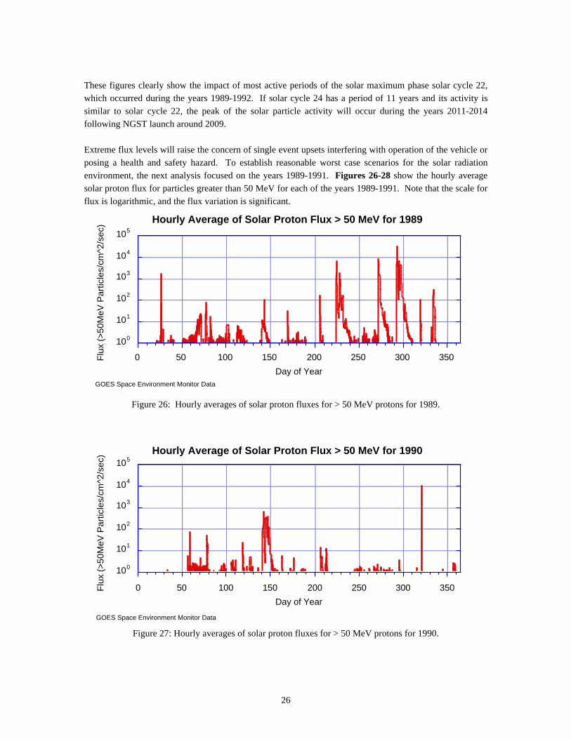
These figures clearly show the impact of most active periods of the solar maximum phase solar cycle 22,which occurred during the years 1989-1992. If solar cycle 24 has a period of 11 years and its activity issimilar to solar cycle 22, the peak of the solar particle activity will occur during the years 2011-2014following NGST launch around 2009.

Extreme flux levels will raise the concern of single event upsets interfering with operation of the vehicle orposing a health and safety hazard. To establish reasonable worst case scenarios for the solar radiationenvironment, the next analysis focused on the years 1989-1991. Figures 26-28 show the hourly averagesolar proton flux for particles greater than 50 MeV for each of the years 1989-1991. Note that the scale forflux is logarithmic, and the flux variation is significant.

100

101

102

103

104

105

0 50 100 150 200 250 300 350

Hourly Average of Solar Proton Flux > 50 MeV for 1989

Flu

x (>

50M

eV P

artic

les/

cm^2

/sec

)

Day of YearGOES Space Environment Monitor Data

Figure 26: Hourly averages of solar proton fluxes for > 50 MeV protons for 1989.

100

101

102

103

104

105

0 50 100 150 200 250 300 350


Flu

x (>

50M

eV P

artic

les/

cm^2

/sec

)

Day of Year

GOES Space Environment Monitor Data


27

100

101

102

103

104

105

0 50 100 150 200 250 300 350


Flu

x (>

50M

eV P

artic

les/

cm^2

/sec

)

Day of Year



Moderate flux levels will affect the ability of NGST to observe dim targets with long exposures. Thegalactic background flux is 5 particles/cm2/s at L2, so NGST will be configured to operate in thisenvironment. To address the problem of observation interference during solar particle events, thedistributions of the solar proton flux counts for 1989, 1990, and 1991 were estimated. During these solarmaximum years, the solar proton flux will vary significantly and will increase the total flux by severalparticles for a large portion of the year. Figures 29 and 30 show the cumulative distributions of solarproton flux for particles greater than 30 and 50 MeV for 1989, 1990, and 1991, and the average of theseyears.. These figures show that, for an average of almost two months for each year of solar maximum, thesolar proton flux will exceed 5 particles/cm2/s for > 30 MeV protons (or over one month per year for > 50MeV protons).

0 10 20 30 40 50 600

15

30

45

60

75

90

Cumulative Distribution of Solar Proton Flux > 30 MeVfor Peak Solar Cycle Years 1989-1991

1989 Flux 1990 Flux 1991 Flux Avg. Flux

0

15

30

45

60

75

90

Flux (>50 MeV particles/cm^2/sec)

Day

s of

Yea

r


Figure 29: Distribution of solar proton flux counts at > 30 MeV

28

0 5 10 15 200

15

30

45

60

75

90

Cumulative Distribution of Solar Proton Flux > 50 MeVfor Peak Solar Cycle Years 1989-1991

1989 Flux 1990 Flux 1991 Flux Avg. Flux

0

15

30

45

60

75

90

Flux (>50 MeV particles/cm^2/sec)

Day

s of

Yea

r


Figure 30: Distribution of solar proton flux counts at > 50 MeV.

VIII. Spacecraft Charging and Discharging

Surface charging and deep dielectric charging must also be evaluated for the NGST mission. Both arepotentially a problem in transfer trajectories that take long loops through the Van Allen belts. During theseloops, the spacecraft can accumulate high levels of electron build-up on spacecraft surfaces (low energyelectrons) in the dielectrics (high energy electrons). When the transfer trajectory of NGST is known inmore detail, the particle accumulation profiles must be estimated and analyzed for possible surface anddeep dielectric charging effects.

At L2 there is also concern that surface charges can build up due to the differential in the plasma during thepasses in and out of the magnetotail. This analysis should be performed when the plasma model becomesavailable.

IX. Summary

A top-level radiation environment specification was presented for the NGST mission. Although theenvironment is considered “moderate”, the environment poses challenges to mission designers because ofits highly variable nature caused by activity on the sun.

Spacecraft and instrument designers must be made aware that some newer technologies and commercial-off-the-shelf (COTS) devices are very soft to radiation effects. COTS devices that lose functionality at5 krads of dose are not uncommon. One extremely large solar proton event can cause enough displacementdamage degradation in some optocoupler devices to cause failure. Increasingly, single event effects requirecareful part selection and mitigation schemes. With its full exposure to galactic cosmic heavy ions andparticles from solar events, NGST must have a carefully planned radiation engineering program.

29

X. References

[1] A. Holmes-Siedle and L. Adams, Handbook of Radiation Effects, p. 16, Oxford University Press,Oxford, 1993.

[2] A. R. Frederickson, “Upsets Related to Spacecraft Charging,” IEEE Trans. on Nucl. Science, Vol.43, No. 2, pp. 426-441, April 1996.

[3] F.M. Ipavich et al., (in press JGR 1997), Space Physics Group, University of Maryland, “TheSolar Wind Proton Monitor on the SOHO Spacecraft,” [WWW Dosument], URLhttp://umtof.umd.edu/papers/pml.htm

[4] L. A. Frank, et al., “The Comprehensive Plasma Instrumentation (CPI) for the GEOTAILSpacecraft,” J. Geomag. Geoelec., Vol. 46, pp. 23-37, 1994.

[5] D. M. Sawyer and J. I. Vette, “AP-8 Trapped Proton Environment,” NSSDC/WDC-A-R&S 76-06,NASA/Goddard Space Flight Center, Greenbelt, MD, December 1991.

[6] J. I. Vette, “The AE-8 Trapped Electron Model Environment,” NSSDC/WDC-A-R&S 91-24,NASA/Goddard Space Flight Center, Greenbelt, MD, November 1991.

[7] M. A. Xapsos, J. L. Barth, E. G. Stassinopoulos, G. P. Summers, E.A. Burke, G. B. Gee, “Modelfor Prediction of Solar Proton Events”, to be published in Proceedings of the 1999 SpaceEnvironment and Effects Workshop, Farnborough, UK.

[8] E. G. Stassinopoulos, “SOLPRO: A Computer Code to Calculate Probabilistic Energetic SolarFlare Protons,” NSSDC 74-11, NASA/Goddard Space Flight Center, Greenbelt, MD, April 1975.

[9] J. Feynman, T. P. Armstrong, L. Dao-Gibner, and S. Silverman, “New Interplanetary ProtonFluence Model,” J. Spacecraft, Vol. 27 No. 24, pp 403-410, July-August 1990.

[10] A. J. Tylka, J. H. Adams, Jr., P. R. Boberg, W. F. Dietrich, E.O. Flueckiger, E.L. Petersen, M.A.Shea, D.F. Smart, and E.C. Smith, “CREME96: A Revision of the Cosmic Ray Effects on Micro-Electronics Code: to be published in IEEE Trans. On Nuc. Sci., December 1997.

[11] GOES home page - http://julius.ngdc.noaa.gov:8080/production/html/GOES/index.html

A-1

Appendices

Table A1Spacecraft Incident Solar Proton Fluences for 1 Solar Active Years

Values Do Not Include Design Margins

Energy Confidence Level(>MeV) 80% 85% 90% 95% 99%

1 1.19E+11 1.47E+11 1.91E+11 2.81E+11 5.83E+11

3 4.18E+10 5.17E+10 6.76E+10 1.01E+11 2.12E+11

5 2.41E+10 3.05E+10 4.08E+10 6.30E+10 1.42E+11

7 1.68E+10 2.16E+10 2.96E+10 4.73E+10 1.14E+11

10 9.84E+09 1.33E+10 1.95E+10 3.44E+10 9.94E+10

15 5.61E+09 7.69E+09 1.14E+10 2.06E+10 6.20E+10

20 3.55E+09 4.93E+09 7.44E+09 1.37E+10 4.31E+10

25 2.43E+09 3.43E+09 5.28E+09 1.00E+10 3.34E+10

30 1.75E+09 2.52E+09 3.97E+09 7.79E+09 2.76E+10

35 1.32E+09 1.93E+09 3.13E+09 6.37E+09 2.42E+10

40 1.03E+09 1.53E+09 2.54E+09 5.36E+09 2.18E+10

45 8.07E+08 1.22E+09 2.06E+09 4.45E+09 1.90E+10

50 6.39E+08 9.74E+08 1.66E+09 3.65E+09 1.60E+10

55 5.10E+08 7.82E+08 1.34E+09 2.97E+09 1.32E+10

60 4.10E+08 6.30E+08 1.08E+09 2.40E+09 1.07E+10

70 2.73E+08 4.19E+08 7.17E+08 1.59E+09 7.07E+09

80 1.90E+08 2.90E+08 4.94E+08 1.09E+09 4.81E+09

90 1.36E+08 2.09E+08 3.56E+08 7.87E+08 3.48E+09

100 1.00E+08 1.54E+08 2.64E+08 5.87E+08 2.63E+09

125 6.05E+07 9.28E+07 1.59E+08 3.54E+08 1.59E+09

150 3.91E+07 6.01E+07 1.03E+08 2.29E+08 1.03E+09

175 2.68E+07 4.11E+07 7.06E+07 1.57E+08 7.03E+08

200 1.92E+07 2.94E+07 5.05E+07 1.12E+08 5.03E+08

225 1.41E+07 2.17E+07 3.72E+07 8.28E+07 3.71E+08

250 1.07E+07 1.64E+07 2.81E+07 6.26E+07 2.80E+08

275 8.25E+06 1.27E+07 2.17E+07 4.83E+07 2.16E+08

300 6.48E+06 9.96E+06 1.71E+07 3.80E+07 1.70E+08

A-2




1 5.93E+11 6.66E+11 7.71E+11 9.58E+11 1.44E+12

3 2.10E+11 2.37E+11 2.76E+11 3.45E+11 5.25E+11

5 1.27E+11 1.46E+11 1.73E+11 2.23E+11 3.60E+11

7 9.28E+10 1.08E+11 1.31E+11 1.74E+11 2.97E+11

10 6.21E+10 7.63E+10 9.90E+10 1.45E+11 2.99E+11

15 3.64E+10 4.54E+10 5.98E+10 8.99E+10 1.93E+11

20 2.37E+10 3.00E+10 4.02E+10 6.20E+10 1.40E+11

25 1.68E+10 2.16E+10 2.97E+10 4.74E+10 1.14E+11

30 1.26E+10 1.65E+10 2.32E+10 3.86E+10 1.00E+11

35 9.79E+09 1.32E+10 1.91E+10 3.32E+10 9.36E+10

40 7.83E+09 1.08E+10 1.61E+10 2.92E+10 8.91E+10

45 6.26E+09 8.76E+09 1.33E+10 2.49E+10 8.04E+10

50 5.01E+09 7.07E+09 1.09E+10 2.07E+10 6.93E+10

55 4.02E+09 5.71E+09 8.86E+09 1.70E+10 5.79E+10

60 3.24E+09 4.61E+09 7.17E+09 1.38E+10 4.73E+10

70 2.16E+09 3.06E+09 4.75E+09 9.11E+09 3.10E+10

80 1.49E+09 2.11E+09 3.26E+09 6.23E+09 2.10E+10

90 1.07E+09 1.52E+09 2.35E+09 4.50E+09 1.52E+10

100 7.92E+08 1.13E+09 1.75E+09 3.38E+09 1.16E+10

125 4.78E+08 6.79E+08 1.06E+09 2.04E+09 6.99E+09

150 3.09E+08 4.40E+08 6.85E+08 1.32E+09 4.52E+09

175 2.12E+08 3.01E+08 4.69E+08 9.04E+08 3.10E+09

200 1.51E+08 2.15E+08 3.35E+08 6.47E+08 2.22E+09

225 1.12E+08 1.59E+08 2.47E+08 4.77E+08 1.63E+09

250 8.44E+07 1.20E+08 1.87E+08 3.60E+08 1.24E+09

275 6.52E+07 9.27E+07 1.44E+08 2.78E+08 9.53E+08

300 5.12E+07 7.29E+07 1.13E+08 2.19E+08 7.50E+08

A-3




1 8.11E+11 8.97E+11 1.02E+12 1.23E+12 1.75E+12

3 2.88E+11 3.20E+11 3.64E+11 4.42E+11 6.36E+11

5 1.75E+11 1.97E+11 2.29E+11 2.86E+11 4.34E+11

7 1.29E+11 1.47E+11 1.74E+11 2.23E+11 3.57E+11

10 8.85E+10 1.07E+11 1.35E+11 1.90E+11 3.64E+11

15 5.23E+10 6.37E+10 8.18E+10 1.18E+11 2.37E+11

20 3.43E+10 4.24E+10 5.54E+10 8.22E+10 1.73E+11

25 2.45E+10 3.09E+10 4.13E+10 6.36E+10 1.42E+11

30 1.85E+10 2.39E+10 3.28E+10 5.24E+10 1.27E+11

35 1.46E+10 1.93E+10 2.73E+10 4.57E+10 1.20E+11

40 1.18E+10 1.59E+10 2.32E+10 4.06E+10 1.16E+11

45 9.49E+09 1.30E+10 1.94E+10 3.50E+10 1.06E+11

50 7.61E+09 1.05E+10 1.59E+10 2.93E+10 9.17E+10

55 6.12E+09 8.53E+09 1.30E+10 2.41E+10 7.68E+10

60 4.94E+09 6.89E+09 1.05E+10 1.96E+10 6.29E+10

70 3.28E+09 4.57E+09 6.94E+09 1.29E+10 4.11E+10

80 2.27E+09 3.15E+09 4.76E+09 8.79E+09 2.78E+10

90 1.63E+09 2.27E+09 3.44E+09 6.36E+09 2.02E+10

100 1.21E+09 1.68E+09 2.57E+09 4.79E+09 1.54E+10

125 7.27E+08 1.02E+09 1.55E+09 2.89E+09 9.29E+09

150 4.71E+08 6.58E+08 1.00E+09 1.87E+09 6.02E+09

175 3.22E+08 4.50E+08 6.86E+08 1.28E+09 4.12E+09

200 2.31E+08 3.22E+08 4.91E+08 9.15E+08 2.95E+09

225 1.70E+08 2.37E+08 3.62E+08 6.75E+08 2.17E+09

250 1.29E+08 1.80E+08 2.73E+08 5.10E+08 1.64E+09

275 9.92E+07 1.39E+08 2.11E+08 3.94E+08 1.27E+09

300 7.80E+07 1.09E+08 1.66E+08 3.10E+08 9.97E+08

A-4

Table A4Integral Solar Proton Fluence Levels Behind Solid Sphere Aluminum Shields

1 Active Solar Year – 95% Confidence LevelValues Do Not Include Design Margins

Shielded Solar Proton FluencesDegraded Energy 50 mils Al

(1.27 mm)100 mils Al(2.54 mm)

200 mils Al(5.08 mm)


> MeV #/cm2 #/cm2 #/cm2 #/cm2

0.10 2.02E+10 1.13E+10 6.68E+09 2.81E+09

0.13 2.02E+10 1.13E+10 6.68E+09 2.81E+09

0.16 2.02E+10 1.13E+10 6.68E+09 2.81E+09

0.20 2.01E+10 1.13E+10 6.68E+09 2.81E+09

0.25 2.01E+10 1.13E+10 6.68E+09 2.81E+09

0.32 2.01E+10 1.13E+10 6.68E+09 2.81E+09

0.40 2.01E+10 1.13E+10 6.68E+09 2.81E+09

0.50 2.01E+10 1.13E+10 6.67E+09 2.81E+09

0.63 2.01E+10 1.13E+10 6.67E+09 2.81E+09

0.79 2.00E+10 1.13E+10 6.67E+09 2.81E+09

1.00 2.00E+10 1.13E+10 6.66E+09 2.81E+09

1.26 1.99E+10 1.13E+10 6.66E+09 2.81E+09

1.58 1.98E+10 1.12E+10 6.65E+09 2.81E+09

2.00 1.97E+10 1.12E+10 6.64E+09 2.80E+09

2.51 1.94E+10 1.11E+10 6.62E+09 2.80E+09

3.16 1.91E+10 1.10E+10 6.59E+09 2.79E+09

3.98 1.86E+10 1.09E+10 6.55E+09 2.78E+09

5.01 1.81E+10 1.07E+10 6.49E+09 2.76E+09

6.31 1.72E+10 1.04E+10 6.40E+09 2.74E+09

7.94 1.60E+10 1.00E+10 6.27E+09 2.70E+09

10.00 1.46E+10 9.50E+09 6.12E+09 2.65E+09

12.60 1.29E+10 8.86E+09 5.88E+09 2.57E+09

15.80 1.10E+10 8.01E+09 5.56E+09 2.44E+09

20.00 9.18E+09 7.06E+09 5.15E+09 2.28E+09

25.10 7.40E+09 6.06E+09 4.54E+09 2.05E+09

31.60 5.87E+09 5.01E+09 3.84E+09 1.78E+09

39.80 4.43E+09 3.82E+09 2.97E+09 1.45E+09

50.10 2.95E+09 2.61E+09 2.05E+09 1.10E+09

63.10 1.69E+09 1.56E+09 1.28E+09 7.81E+08

79.40 8.86E+08 8.54E+08 7.55E+08 5.19E+08

100.00 4.57E+08 4.50E+08 4.28E+08 3.44E+08

126.00 2.55E+08 2.53E+08 2.47E+08 2.11E+08

158.00 1.33E+08 1.32E+08 1.30E+08 1.16E+08

200.00 5.86E+07 5.84E+07 5.79E+07 5.36E+07

251.00 1.64E+07 1.64E+07 1.64E+07 1.50E+07

A-5


5 Active Solar Years – 95% Confidence LevelValues Do Not Include Design Margins

Shielded Solar Proton FluencesDegraded Energy 50 mils Al

(1.27 mm)100 mils Al(2.54 mm)



> MeV #/cm2 #/cm2 #/cm2 #/cm2

0.10 8.78E+10 5.21E+10 3.39E+10 1.61E+10

0.13 8.77E+10 5.21E+10 3.39E+10 1.61E+10

0.16 8.77E+10 5.21E+10 3.39E+10 1.61E+10

0.20 8.77E+10 5.21E+10 3.39E+10 1.61E+10

0.25 8.77E+10 5.21E+10 3.39E+10 1.61E+10

0.32 8.76E+10 5.21E+10 3.39E+10 1.61E+10

0.40 8.76E+10 5.21E+10 3.39E+10 1.61E+10

0.50 8.75E+10 5.20E+10 3.39E+10 1.61E+10

0.63 8.74E+10 5.20E+10 3.38E+10 1.61E+10

0.79 8.73E+10 5.20E+10 3.38E+10 1.61E+10

1.00 8.71E+10 5.19E+10 3.38E+10 1.61E+10

1.26 8.68E+10 5.18E+10 3.38E+10 1.61E+10

1.58 8.64E+10 5.17E+10 3.38E+10 1.61E+10

2.00 8.58E+10 5.15E+10 3.37E+10 1.61E+10

2.51 8.49E+10 5.13E+10 3.37E+10 1.60E+10

3.16 8.36E+10 5.09E+10 3.35E+10 1.60E+10

3.98 8.17E+10 5.03E+10 3.34E+10 1.59E+10

5.01 7.94E+10 4.94E+10 3.32E+10 1.58E+10

6.31 7.59E+10 4.84E+10 3.28E+10 1.57E+10

7.94 7.12E+10 4.69E+10 3.23E+10 1.55E+10

10.00 6.52E+10 4.48E+10 3.17E+10 1.52E+10

12.60 5.86E+10 4.23E+10 3.08E+10 1.47E+10

15.80 5.12E+10 3.89E+10 2.95E+10 1.40E+10

20.00 4.38E+10 3.52E+10 2.79E+10 1.31E+10

25.10 3.68E+10 3.14E+10 2.50E+10 1.18E+10

31.60 3.09E+10 2.72E+10 2.16E+10 1.02E+10

39.80 2.47E+10 2.15E+10 1.70E+10 8.28E+09

50.10 1.69E+10 1.50E+10 1.18E+10 6.29E+09

63.10 9.69E+09 8.91E+09 7.33E+09 4.46E+09

79.40 5.05E+09 4.88E+09 4.31E+09 2.99E+09

100.00 2.63E+09 2.59E+09 2.47E+09 1.98E+09

126.00 1.47E+09 1.46E+09 1.42E+09 1.21E+09

158.00 7.63E+08 7.59E+08 7.49E+08 6.68E+08

200.00 3.38E+08 3.37E+08 3.34E+08 3.09E+08

251.00 9.42E+07 9.42E+07 9.42E+07 8.62E+07

A-6


7 Active Solar Years – 95% Confidence LevelValues Do Not Include Design Margins

Shielded Solar Proton FluencesDegraded Energy

50 mils Al(1.27 mm)




> MeV #/cm2 #/cm2 #/cm2 #/cm2

0.10 1.15E+11 6.93E+10 4.63E+10 2.29E+10

0.13 1.15E+11 6.93E+10 4.63E+10 2.29E+10

0.16 1.15E+11 6.93E+10 4.63E+10 2.29E+10

0.20 1.15E+11 6.93E+10 4.63E+10 2.29E+10

0.25 1.15E+11 6.93E+10 4.63E+10 2.29E+10

0.32 1.15E+11 6.93E+10 4.63E+10 2.29E+10

0.40 1.15E+11 6.93E+10 4.63E+10 2.29E+10

0.50 1.15E+11 6.92E+10 4.62E+10 2.29E+10

0.63 1.15E+11 6.92E+10 4.62E+10 2.28E+10

0.79 1.15E+11 6.92E+10 4.62E+10 2.28E+10

1.00 1.14E+11 6.91E+10 4.62E+10 2.28E+10

1.26 1.14E+11 6.90E+10 4.62E+10 2.28E+10

1.58 1.13E+11 6.88E+10 4.61E+10 2.28E+10

2.00 1.13E+11 6.86E+10 4.61E+10 2.28E+10

2.51 1.11E+11 6.83E+10 4.60E+10 2.27E+10

3.16 1.10E+11 6.78E+10 4.59E+10 2.27E+10

3.98 1.07E+11 6.70E+10 4.57E+10 2.26E+10

5.01 1.04E+11 6.59E+10 4.54E+10 2.25E+10

6.31 1.00E+11 6.45E+10 4.50E+10 2.23E+10

7.94 9.39E+10 6.26E+10 4.43E+10 2.20E+10

10.00 8.62E+10 6.00E+10 4.36E+10 2.15E+10

12.60 7.77E+10 5.68E+10 4.24E+10 2.09E+10

15.80 6.84E+10 5.25E+10 4.08E+10 1.99E+10

20.00 5.88E+10 4.79E+10 3.87E+10 1.86E+10

25.10 5.00E+10 4.31E+10 3.50E+10 1.67E+10

31.60 4.27E+10 3.78E+10 3.05E+10 1.45E+10

39.80 3.46E+10 3.04E+10 2.41E+10 1.17E+10

50.10 2.39E+10 2.12E+10 1.67E+10 8.88E+09

63.10 1.37E+10 1.26E+10 1.04E+10 6.30E+09

79.40 7.13E+09 6.88E+09 6.08E+09 4.23E+09

100.00 3.72E+09 3.67E+09 3.50E+09 2.81E+09

126.00 2.08E+09 2.07E+09 2.01E+09 1.72E+09

158.00 1.08E+09 1.08E+09 1.06E+09 9.46E+08

200.00 4.79E+08 4.77E+08 4.73E+08 4.37E+08

251.00 1.34E+08 1.34E+08 1.34E+08 1.23E+08

A-7

Table A7Total Ionizing Dose at the Center of Aluminum Spheres Due to Solar Proton Events

95% Confidence LevelValues Do Not Include Design Margins

Aluminum Shield Thickness 1 SolarActive Year

5 SolarActive Years

7 SolarActive Years

g/cm2 mm mils krads-si krads-si krads-si

0.03 0.11 4.37 9.06E+01 2.92E+02 3.72E+02

0.04 0.15 5.83 6.89E+01 2.22E+02 2.82E+02

0.05 0.19 7.29 5.41E+01 1.71E+02 2.17E+02

0.06 0.22 8.75 4.64E+01 1.47E+02 1.87E+02

0.08 0.30 11.67 3.68E+01 1.15E+02 1.44E+02

0.10 0.37 14.58 3.00E+01 9.31E+01 1.15E+02

0.15 0.56 21.87 2.23E+01 8.24E+01 1.06E+02

0.20 0.74 29.16 1.78E+01 7.19E+01 9.36E+01

0.30 1.11 43.74 1.14E+01 4.69E+01 6.07E+01

0.40 1.48 58.31 8.37E+00 3.45E+01 4.45E+01

0.50 1.85 72.91 6.18E+00 2.57E+01 3.32E+01

0.60 2.22 87.48 5.04E+00 2.09E+01 2.70E+01

0.80 2.96 116.65 3.53E+00 1.50E+01 1.96E+01

1.00 3.70 145.83 2.69E+00 1.17E+01 1.53E+01

1.25 4.63 182.28 2.04E+00 9.21E+00 1.21E+01

1.50 5.56 218.74 1.72E+00 8.09E+00 1.08E+01

1.75 6.48 255.16 1.48E+00 7.32E+00 9.89E+00

2.00 7.41 291.61 1.33E+00 6.88E+00 9.37E+00

2.50 9.26 364.53 1.05E+00 5.74E+00 7.98E+00

3.00 11.11 437.40 8.64E-01 4.85E+00 6.86E+00

3.50 12.96 510.24 6.91E-01 3.95E+00 5.59E+00

4.00 14.81 583.07 5.60E-01 3.23E+00 4.60E+00

4.50 16.67 656.30 4.45E-01 2.56E+00 3.65E+00

5.00 18.52 729.13 3.60E-01 2.06E+00 2.93E+00

5.50 20.37 801.97 3.08E-01 1.77E+00 2.51E+00

6.00 22.22 874.80 2.53E-01 1.45E+00 2.05E+00

6.50 24.07 947.64 2.13E-01 1.22E+00 1.72E+00

7.00 25.93 1020.87 1.83E-01 1.04E+00 1.47E+00

7.50 27.78 1093.70 1.57E-01 8.97E-01 1.26E+00

8.00 29.63 1166.54 1.39E-01 7.88E-01 1.11E+00

8.50 31.48 1239.37 1.21E-01 6.90E-01 9.72E-01

9.00 33.33 1312.20 1.07E-01 6.11E-01 8.62E-01

9.50 35.19 1385.43 9.32E-02 5.34E-01 7.55E-01

10.00 37.04 1458.27 7.84E-02 4.51E-01 6.40E-01

12.50 46.30 1822.83 5.69E-02 3.28E-01 4.64E-01

15.00 55.56 2187.40 4.18E-02 2.41E-01 3.41E-01

20.00 74.07 2916.14 2.44E-02 1.41E-01 1.99E-01

25.00 92.59 3645.28 1.55E-02 8.88E-02 1.26E-01

30.00 111.10 4374.02 1.10E-02 6.33E-02 8.96E-02

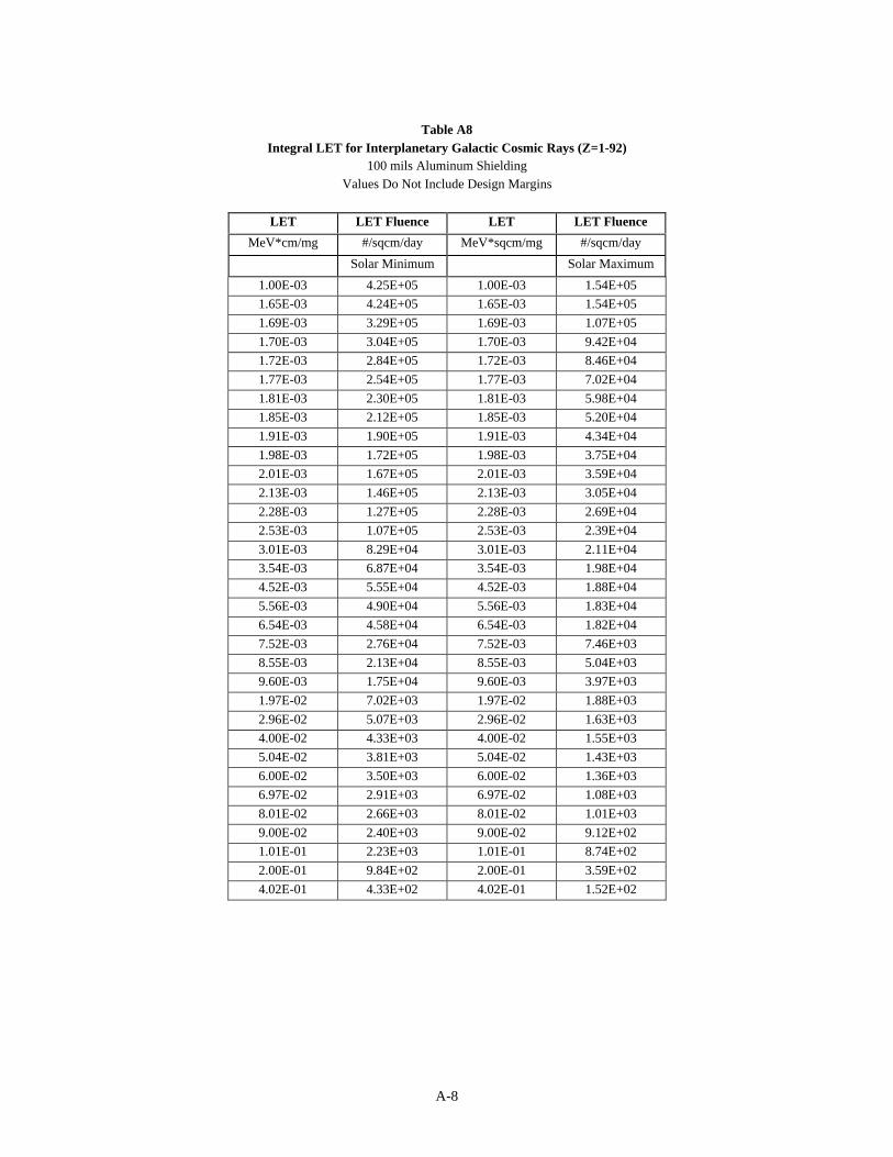
A-8

Table A8Integral LET for Interplanetary Galactic Cosmic Rays (Z=1-92)

100 mils Aluminum ShieldingValues Do Not Include Design Margins

LET LET Fluence LET LET Fluence

MeV*cm/mg #/sqcm/day MeV*sqcm/mg #/sqcm/day

Solar Minimum Solar Maximum

1.00E-03 4.25E+05 1.00E-03 1.54E+051.65E-03 4.24E+05 1.65E-03 1.54E+051.69E-03 3.29E+05 1.69E-03 1.07E+051.70E-03 3.04E+05 1.70E-03 9.42E+041.72E-03 2.84E+05 1.72E-03 8.46E+041.77E-03 2.54E+05 1.77E-03 7.02E+041.81E-03 2.30E+05 1.81E-03 5.98E+041.85E-03 2.12E+05 1.85E-03 5.20E+041.91E-03 1.90E+05 1.91E-03 4.34E+041.98E-03 1.72E+05 1.98E-03 3.75E+042.01E-03 1.67E+05 2.01E-03 3.59E+042.13E-03 1.46E+05 2.13E-03 3.05E+042.28E-03 1.27E+05 2.28E-03 2.69E+042.53E-03 1.07E+05 2.53E-03 2.39E+043.01E-03 8.29E+04 3.01E-03 2.11E+043.54E-03 6.87E+04 3.54E-03 1.98E+044.52E-03 5.55E+04 4.52E-03 1.88E+045.56E-03 4.90E+04 5.56E-03 1.83E+046.54E-03 4.58E+04 6.54E-03 1.82E+047.52E-03 2.76E+04 7.52E-03 7.46E+038.55E-03 2.13E+04 8.55E-03 5.04E+039.60E-03 1.75E+04 9.60E-03 3.97E+031.97E-02 7.02E+03 1.97E-02 1.88E+032.96E-02 5.07E+03 2.96E-02 1.63E+034.00E-02 4.33E+03 4.00E-02 1.55E+035.04E-02 3.81E+03 5.04E-02 1.43E+036.00E-02 3.50E+03 6.00E-02 1.36E+036.97E-02 2.91E+03 6.97E-02 1.08E+038.01E-02 2.66E+03 8.01E-02 1.01E+039.00E-02 2.40E+03 9.00E-02 9.12E+021.01E-01 2.23E+03 1.01E-01 8.74E+022.00E-01 9.84E+02 2.00E-01 3.59E+024.02E-01 4.33E+02 4.02E-01 1.52E+02

A-9

Table A8 (Continued)Integral LET for Interplanetary Galactic Cosmic Rays (Z=1-92)


LET LET Fluence LET LET Fluence

MeV*cm/mg #/sqcm/day MeV*sqcm/mg #/sqcm/day

Solar Minimum Solar Maximum

6.03E-01 2.90E+02 6.03E-01 1.10E+027.96E-01 2.23E+02 7.96E-01 8.84E+011.00E+00 1.79E+02 1.00E+00 7.22E+012.01E+00 3.39E+01 2.01E+00 5.88E+003.02E+00 1.43E+01 3.02E+00 2.03E+003.99E+00 7.76E+00 3.99E+00 1.02E+005.03E+00 4.59E+00 5.03E+00 5.81E-015.99E+00 3.07E+00 5.99E+00 3.80E-018.00E+00 1.55E+00 8.00E+00 1.90E-011.01E+01 9.00E-01 1.01E+01 1.10E-011.11E+01 7.17E-01 1.11E+01 8.75E-021.20E+01 5.76E-01 1.20E+01 7.04E-021.30E+01 4.67E-01 1.30E+01 5.71E-021.40E+01 3.85E-01 1.40E+01 4.72E-021.50E+01 3.16E-01 1.50E+01 3.88E-021.60E+01 2.61E-01 1.60E+01 3.20E-021.70E+01 2.20E-01 1.70E+01 2.71E-021.80E+01 1.85E-01 1.80E+01 2.27E-021.91E+01 1.54E-01 1.91E+01 1.89E-022.00E+01 1.30E-01 2.00E+01 1.60E-022.49E+01 4.45E-02 2.49E+01 5.50E-033.00E+01 6.27E-04 3.00E+01 8.18E-053.49E+01 6.86E-05 3.49E+01 1.06E-054.01E+01 4.18E-05 4.01E+01 6.50E-064.50E+01 2.83E-05 4.50E+01 4.42E-065.00E+01 2.00E-05 5.00E+01 3.13E-065.06E+01 1.92E-05 5.06E+01 3.00E-065.55E+01 1.34E-05 5.55E+01 2.11E-066.02E+01 9.38E-06 6.02E+01 1.49E-066.53E+01 6.32E-06 6.53E+01 1.01E-067.00E+01 4.40E-06 7.00E+01 7.01E-077.50E+01 2.83E-06 7.50E+01 4.52E-078.04E+01 1.65E-06 8.04E+01 2.63E-078.52E+01 7.71E-07 8.52E+01 1.23E-079.03E+01 1.94E-07 9.03E+01 3.10E-089.57E+01 2.88E-08 9.57E+01 4.60E-091.00E+02 1.19E-08 1.00E+02 1.89E-091.01E+02 5.27E-09 1.01E+02 8.41E-101.03E+02 2.54E-09 1.03E+02 4.05E-10

A-10

Table A9Integral LET for the October 1989 Solar Particle Event (Z=1-92)


LET LET Fluence LET Fluence LET FluenceMeV*cm2/mg #/cm2/s #/cm2/s #/cm2/s

Average Over Peak Average Over Worst Day Average Over Worst Week

1.00E-03 1.93E+05 5.21E+04 1.15E+042.01E-03 1.93E+05 5.21E+04 1.15E+043.01E-03 1.93E+05 5.20E+04 1.14E+044.02E-03 1.92E+05 5.17E+04 1.13E+045.01E-03 1.90E+05 5.11E+04 1.11E+046.03E-03 1.86E+05 5.02E+04 1.08E+047.02E-03 1.82E+05 4.90E+04 1.05E+047.97E-03 1.77E+05 4.76E+04 1.01E+048.95E-03 1.71E+05 4.60E+04 9.68E+031.01E-02 1.64E+05 4.40E+04 9.19E+031.99E-02 9.60E+04 2.55E+04 5.07E+032.99E-02 5.39E+04 1.43E+04 2.78E+034.00E-02 3.23E+04 8.56E+03 1.65E+034.98E-02 2.11E+04 5.59E+03 1.07E+036.00E-02 1.45E+04 3.84E+03 7.33E+026.97E-02 1.06E+04 2.81E+03 5.34E+028.01E-02 7.91E+03 2.09E+03 3.96E+029.00E-02 6.16E+03 1.63E+03 3.08E+029.99E-02 4.90E+03 1.29E+03 2.44E+022.00E-01 9.50E+02 2.51E+02 4.67E+013.01E-01 3.15E+02 8.31E+01 1.53E+014.02E-01 1.25E+02 3.32E+01 6.08E+005.01E-01 3.82E+01 1.01E+01 1.80E+006.03E-01 1.86E+01 4.94E+00 8.78E-017.01E-01 1.35E+01 3.58E+00 6.52E-018.05E-01 9.85E+00 2.62E+00 4.91E-019.04E-01 7.55E+00 2.02E+00 3.87E-011.00E+00 5.88E+00 1.57E+00 3.10E-012.01E+00 7.49E-01 2.06E-01 5.99E-023.02E+00 4.11E-01 1.13E-01 3.33E-023.99E+00 2.64E-01 7.29E-02 2.14E-025.03E+00 1.74E-01 4.80E-02 1.42E-026.06E+00 1.21E-01 3.36E-02 9.92E-037.04E+00 8.68E-02 2.40E-02 7.11E-038.00E+00 6.39E-02 1.77E-02 5.26E-038.99E+00 5.04E-02 1.40E-02 4.13E-031.01E+01 3.85E-02 1.07E-02 3.15E-032.00E+01 5.75E-03 1.60E-03 4.63E-042.52E+01 2.14E-03 5.95E-04 1.72E-04

A-11

Table A9 (Continued)Integral LET for the October 1989 Solar Particle Event (Z=1-92)


LET LET Fluence LET Fluence LET FluenceMeV*cm2/mg #/cm2/s #/cm2/s #/cm2/s


3.00E+01 1.83E-05 5.10E-06 1.55E-063.53E+01 7.23E-07 2.01E-07 7.14E-084.01E+01 3.26E-07 9.08E-08 3.43E-084.50E+01 1.95E-07 5.44E-08 2.12E-085.00E+01 1.36E-07 3.78E-08 1.48E-085.55E+01 8.43E-08 2.35E-08 9.31E-096.02E+01 4.92E-08 1.37E-08 5.58E-096.53E+01 3.28E-08 9.12E-09 3.75E-097.00E+01 2.49E-08 6.92E-09 2.84E-097.50E+01 1.80E-08 5.00E-09 2.04E-098.04E+01 1.20E-08 3.34E-09 1.36E-098.52E+01 6.69E-09 1.86E-09 7.56E-109.03E+01 2.03E-09 5.64E-10 2.29E-109.46E+01 1.33E-10 3.71E-11 1.51E-111.00E+02 5.01E-11 1.39E-11 5.66E-121.01E+02 2.22E-11 6.19E-12 2.51E-121.03E+02 1.07E-11 2.99E-12 1.21E-12

A-12

Table A10Differential Fluxes from Solar Proton Events

100 mils Aluminum Shielding, CREME96Note: Spectra were cut off at E =1 MeV and E=1000 MeV


Energy Proton Flux Proton Flux Proton FluxMeV #/cm2/s #/cm2/s #/cm2/s


1.00 1.75E+03 4.62E+02 8.85E+01

2.00 2.68E+03 7.09E+02 1.36E+02

3.02 3.47E+03 9.17E+02 1.76E+02

4.04 4.11E+03 1.09E+03 2.09E+02

5.04 4.62E+03 1.22E+03 2.36E+02

6.03 5.03E+03 1.33E+03 2.58E+02

7.02 5.33E+03 1.41E+03 2.75E+02

8.06 5.56E+03 1.47E+03 2.88E+02

9.00 5.69E+03 1.51E+03 2.96E+02

10.05 5.76E+03 1.53E+03 3.01E+02

14.99 5.41E+03 1.44E+03 2.92E+02

20.03 4.50E+03 1.21E+03 2.52E+02

24.98 3.57E+03 9.65E+02 2.07E+02

30.31 2.73E+03 7.40E+02 1.64E+02

35.27 2.11E+03 5.75E+02 1.31E+02

40.49 1.61E+03 4.42E+02 1.04E+02

50.50 9.91E+02 2.73E+02 6.79E+01

60.43 6.33E+02 1.75E+02 4.58E+01

70.33 4.20E+02 1.17E+02 3.20E+01

79.63 2.94E+02 8.18E+01 2.33E+01

90.17 2.03E+02 5.65E+01 1.68E+01

100.69 1.44E+02 4.01E+01 1.24E+01

150.25 3.84E+01 1.06E+01 3.80E+00

200.77 1.39E+01 3.79E+00 1.50E+00

299.59 3.32E+00 8.62E-01 3.88E-01

400.31 1.16E+00 2.85E-01 1.39E-01

499.23 4.97E-01 1.16E-01 5.96E-02

605.64 2.07E-01 4.64E-02 2.54E-02

704.94 1.10E-01 2.48E-02 1.44E-02

798.17 6.61E-02 1.48E-02 9.03E-03

903.74 3.95E-02 8.88E-03 5.66E-03

995.41 2.65E-02 5.96E-03 3.94E-03

the radiation environment for the next generation … radiation environment for the next generation...

Documents