the quest for a truly parsimonious airfoil ...eprints.soton.ac.uk/64913/1/sobe_08a.pdf · the quest...

The Quest for a Truly Parsimonious

Airfoil Parameterization Scheme

Andras Sobester∗, Thomas Barrett†

University of Southampton, Southampton, Hampshire, SO17 1BJ, UK

The conceptual phase of the aircraft design process demands a parsimo-

nious description of the airframe geometry. While there is no hard and fast

upper limit on the affordable number of variables, the so-called ‘curse of di-

mensionality’ must always be kept in mind: if a thorough, conceptual level

search of a one-variable space can be accomplished by the evaluation of n can-

didate designs, the same level of thoroughness (however one chooses to define

this) will demand nk evaluations in k-dimensional space. Therefore, to make

the design search tractable and the complexity of the geometry definition at

a level where the effect of the variables can be readily understood by the de-

signer, the number of airframe definition variables should be minimized. This

has an impact on all of the components, perhaps most importantly on airfoil-

type section definitions that feature on all ‘wing-like’ surfaces. It is therefore

imperative to define these sections as parsimoniously as possible. In this pa-

per we examine a series of parameterization schemes, whose chief conception

criterion was conciseness in terms of the number of design variables. Another

constraint we are considering is the ease of implementation in a commercial

off-the-shelf Computer Aided Design engine.

I. Introduction

THE ‘curse of dimensionality’, that is, the observation that the size of a k-dimensional spaceobserved at q levels is O(qk), presents conceptual designers with a significant challenge in terms

of reducing the number of design variables. This is especially pressing when it comes to defining airfoilsections, as these feature on every lifting surface on an airframe and therefore are often responsiblefor a significant fraction of the overall number of design variables. This paper presents a number ofpotential airfoil representation formulations designed with low dimensionality as the chief driver.

The search for practically useful parametric airfoils is almost as old as heavier than air flightitself. A plethora of airfoil geometry definition schemes have been proposed over the years and manydifferent criteria could be used to arrange these into a taxonomy. Here, in a brief overview of existingapproaches, we choose to simply position them along a continuum of design variable scopes. In otherwords, we classify them according to the geometrical extent (in terms of the overall size of the airfoil)of the influence of any particular design variable, as this criterion feels the most germane when itcomes to clarifying the place of our proposed schemes in the rather broad context of airfoil descriptionmethodology.

∗Lecturer, Computational Engineering and Design Group, AIAA member.†AIAA Member

1Submitted to the American Institute of Aeronautics and Astronautics

Consider the extremes of this scale. If a computational fluid dynamics mesh is generated around aputative airfoil, one could designate the coordinates of the mesh points falling onto the airfoil surfaceas design variables. Sometimes combined with a related mapping of the rest of the mesh, as well as asmoothness constraint designed to prevent the emergence of ‘jagged’ airfoils, this is a highly successfulscheme when a local improvement is sought in relation to the starting point of the design process. Thesearch can be particularly efficient when adjoint gradients are available at a computational cost thatis independent of problem dimensionality. A classic example is the control theory based formulationof Jameson.1 Clearly, in this case the influence of a design variable is restricted to the immediatevicinity of its corresponding mesh point.

Staying with Jameson’s work, one can also find here an example of the opposite end of the scale,where a design parameter’s scope is the entire airfoil. In Ref. 2 he describes the solution of thepotential flow equations over an airfoil, which results from a circle, via a complex conformal mapping(a mapping, which is, incidentally, also applied to the mesh). A very similar example is that of thewell-known Jukowski airfoil – in both cases the impact of changes to the coordinates of the circle beingmapped can be seen across the entire airfoil.

All other methods populate the span between these two extremes. Indeed, some can take updifferent locations along this continuum, depending on how the designer chooses to implement them.For example, the ‘bump’ functions, introduced by Hicks and Henne3 at the dawn of the computer-aided design age, can be added to the baseline airfoil scaled to the entire chord, or, more locally, to alimited part thereof (see Ref. 4 for an 18-variable example). Another way of controlling the scope ofthe Hicks-Henne parameterisation method is to restrict the range of permitted chordwise movementof the peak of the bump (while the base of the bump rests on the full chord).

Also, to some extent, variable in scope, is the scheme described recently by Kulfan.5 At the heartof her airfoil description lies a generic template, containing a square root term (to ensure a roundleading edge), and a ‘1-x/chord’ term to close the trailing edge (with another term specifying a finitetrailing-edge thickness). The actual parameterisation is encapsulated by a shape function term withvariable flexibility. At its stiffest, the shape function can depend on a single variable – in this casewe can control the nose radius on both the lower and upper surfaces at the same time. It is alsopossible to set up a one variable shape function to control the boat-tail angle. Both of these choicesplace us about half-way down the scope continuum, as the impact of any change affects either thefore or the aft section of the airfoil. More flexible shape functions can come, for example, in the formof a Bernstein-polynomial partition of unity, which gives increasingly finer and, in some sense, morelocalized control of the shape (as an illustration of the flexibility of the shape function, Ref. 5 includes8th order Bernstein polynomial approximations of the RAE2822 airfoil, which take the approximationerrors well below wind tunnel model tolerances).

Let us now consider a few examples of formulations with more specific places on the parameterscope scale. Lepine et al.6 and Painchaud-Ouellet et al.7 use NURBS curves to define their airfoils,where the coordinates and the weights of the control points are the design variables. The significantimpact of each is, of course, restricted to the vicinity of the relevant control point and therefore thisscheme is close to the local end of the scope scale.


6th order polynomials form the basis of the PARSEC formulation.8 Each of the 11 design variablesis connected to a very specific feature of the airfoil: leading edge radius, upper and lower crest location,curvatures at the crests, trailing edge ordinates, thickness, tail direction and wedge angle. This is,therefore also fairly near to the local end of the scale: each variable affects a well-defined section ofthe airfoil.

Near the global end we find the classic 4-digit NACA foils. The variables here refer to specificfeatures of the airfoil (max thickness and its location and maximum camber), but, each of theserefers to both the upper and the lower surface of the airfoil and thus any change in any of thedesign variables has some impact on every point. Also at the global end we find the orthogonal basisfunctions of Robinson and Keane.9 These functions represent features extracted from the NASAPhase 2 supercritical airfoils (described by Harris10) and the variables, which are the weights of thesebases, affect the shape of the entire airfoil.

As we stated at the outset, our main aim here is to consider a number of parsimonious parametricairfoils, that is, section descriptions that can be controlled through a relatively small number ofparameters (accepting inevitable sacrifices in terms of flexibility, i.e., the ability of the parametricairfoil to take up a wide range of shapes).

It is clear that, in terms of the above classification, parametric airfoils suitable for conceptual designcannot be at the local end of the parameter scope scale. We therefore start, in what follows, aroundthe mid-point of the scale, with three schemes that, as we shall see, share a number of features.The simplest of this trio is based on cubic splines (Section II) – this is followed by two B-splinebased schemes (Sections III and IV). We then tackle the global extreme of the scale, via a variabledimensionality formulation based on defining new airfoils in terms of the features of existing, ‘classic’sections (Section V).

II. A Parametric Airfoil Based on Cubic Splines

We begin with a six-variable formulation based on a pair of cubic splines. The main advantage ofthis scheme lies in its simplicity: setup times are minimal in most programming environments and themathematical definition is also simpler than that of the B-spline-based schemes we shall tackle lateron. For these reasons we have found this a rather effective teaching tool. The main drawback is thatit is only suitable for low speed applications – a pair of splines controlled from their endpoints (whichis how we shall construct this parametric section) do not have the flexibility required to generatethe near-flat surface regions found on supercritical airfoils. In what follows we briefly outline themathematical formulation of this airfoil definition method.

Ferguson’s Parametric Splines

The specific spline formulation that forms our starting point is that of The Boeing Company’sJames Ferguson, whose seminal 1964 paper11 lies at the foundation of the curve (and surface) definitionalgorithms built into modern Computer Aided Design (CAD) tools. Although Bezier and others havesubsequently published slightly different and now better known forms of cubics, their basic logic isvery similar to what we now proceed to describe.


Fig. 1 Ferguson spline and its boundary conditions.

We seek a parametric curve S(t) with t ∈ [0, 1], connecting two points S(0) = A and S(1) = B.We impose two tangents on the curve: dS/dt|t=0 = TA and dS/dt|t=1 = TB , as shown in Figure 1.We define the curve as the polynomial

S(t) =3∑

i=0

aiti, t ∈ [0, 1]. (1)

We find the four vectors required to define the curve by setting the endpoint conditions:

A = a0

B = a0 + a1 + a2 + a3 (2)

TA = a1

TB = a1 + 2a2 + 3a3

and by re-arranging:

a0 = A

a1 = TA (3)

a2 = 3[B−A]− 2TA −TA

a3 = 2[A−B] + TA + TB .

Substituting them back into Equation (1) we obtain:

S(t) = A(1− 3t2 + 2t3) + B(3t2 − 2t3) + TA(t− 2t2 + t3) + TB(−t2 + t3), (4)

or in matrix form:

S(t) =[

1 t t2 t3]

1 0 0 00 0 1 0−3 3 −2 −12 −2 1 1

A

B

TA

TB

. (5)

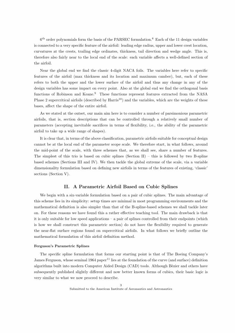
S(t) is, essentially, a Hermitian interpolant and the bracketed factors in equation (4) can be viewedas its basis functions – Figure 2 conveys an intuitive understanding of their effect on the shape of theinterpolant. We now proceed to discuss the suggested airfoil parameterization scheme based on theformulation outlined in the introduction.


0 0.2 0.4 0.6 0.8 1−0.2

0

0.2

0.4

0.6

0.8

1

1.2

t

Her

miti

an b

asis

func

tions A ´

B ´

TA ´

TB ´

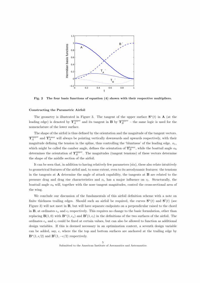
Fig. 2 The four basis functions of equation (4) shown with their respective multipliers.

Constructing the Parametric Airfoil

The geometry is illustrated in Figure 3. The tangent of the upper surface Su(t) in A (at theleading edge) is denoted by Tupper

A and its tangent in B by TupperB – the same logic is used for the

nomenclature of the lower surface.

The shape of the airfoil is thus defined by the orientation and the magnitude of the tangent vectors.Tupper

A and TlowerA will always be pointing vertically downwards and upwards respectively, with their

magnitude defining the tension in the spline, thus controlling the ‘bluntness’ of the leading edge. αc,which might be called the camber angle, defines the orientation of Tlower

B , while the boattail angle αb

determines the orientation of TupperB . The magnitudes (tangent tensions) of these vectors determine

the shape of the middle section of the airfoil.

It can be seen that, in addition to having relatively few parameters (six), these also relate intuitivelyto geometrical features of the airfoil and, to some extent, even to its aerodynamic features: the tensionsin the tangents at A determine the angle of attack capability, the tangents at B are related to thepressure drag and drag rise characteristics and αc has a major influence on cl. Structurally, theboattail angle αb will, together with the nose tangent magnitudes, control the cross-sectional area ofthe wing.

We conclude our discussion of the fundamentals of this airfoil definition scheme with a note onfinite thickness trailing edges. Should such an airfoil be required, the curves Su(t) and Sl(t) (seeFigure 3) will not meet in B, but will have separate endpoints on a perpendicular raised to the chordin B, at ordinates εu and εl respectively. This requires no change to the basic formulation, other thanreplacing B(1, 0) with Bu(1, εu) and Bl(1, εl) in the definitions of the two surfaces of the airfoil. Theordinates εu and εl could be fixed at certain values, but can also be allowed to function as additionaldesign variables. If this is deemed necessary in an optimization context, a seventh design variablecan be added, say, ε, where the the top and bottom surfaces are anchored at the trailing edge byBu(1, ε/2) and Bl(1,−ε/2) respectively.


αc

αb

TB

upper

TB

lower

TA

lower

TA

upper

A B

Su(t)

Sl(t)

Fig. 3 The airfoil parameterization scheme based on two Ferguson splines. The parametric

curves Su(t) and Sl(t) describe the upper and lower surfaces respectively.

As we indicated at the outset, the flexibility of this parametric airfoil may be too limited to re-create certain classes of high speed airfoils. Nevertheless, there are numerous other ‘classic’ shapesthat this simple and robust formulation can approximate rather closely. Such approximations canbe obtained by minimizing some difference metric (e.g., mean squared error) between the parametricairfoil and the target of the approximation, subject to the design variables |Tupper

A |, |TlowerA |, etc.

Here are two examples of parameter sets obtained in this way:

Target airfoil |TupperA | |Tlower

A | |TupperB | |Tlower

B | αc [deg] αb [deg] εl εu

NACA 5410 0.1584 0.1565 2.1241 1.8255 3.8270 11.6983 -0.0032 0.0012

NACA 21012 0.1674 0.2402 2.2482 1.3236 -8.7800 17.2397 -0.0074 -0.0080

The reader interested in more such reconstructions, implementation details, flexibility analysis anda multi-objective design study based on this parametric airfoil, will find these in Ref. 12. We nowmove on to consider another simple parameterisation scheme of the same dimensionality (k = 6), thistime using a set of interpolation points and a more sophisticated geometrical formulation: a B-spline.

III. A B-Spline Based Parametric Airfoil

Constructing an Interpolating B-Spline

Let the following vector curve define a p-th order B-spline:

S(t) =n∑

i=0

Ni,p(t)Pi (6)


for t ∈ [0, 1]. Pi are the (n+1) control points, and Ni,p(t) are the p-th degree B-spline basis functions.The knot vector, T, containing (m + 1) knots, is defined as

T = 0, . . . , 0︸︷︷︸p+1

, tp+1, . . . , tm−p−1, 1, . . . , 1︸︷︷︸p+1

(7)

in which m = n + p + 1. The B-spline basis functions of degree p (order p + 1) are defined as

Ni,p(t) =t− ti

ti+p − tiNi,p−1(t) +

ti+p+1 − t

ti+p+1 − ti+1Ni+1,p−1(t). (8)

Note that this linear combination of lower order basis functions is defined everywhere, though we donot actually need it outside the range defined by the extremities of the knot vector. This recursiveformulation (due to Cox13 and De Boor14) can be pictured intuitively as a triangle, whose apex is thebasis function to be calculated, the two basis functions needed for its calculation are right underneathit and so on. The base of the triangle, which effectively controls the ranges of influence of the controlpoints, is defined as:

Ni,0(t) =

1 if ti ≤ t < ti+1

0 otherwise.(9)

When evaluating the curve S(t), for each t one finds the knot span in which it lies, computes therelevant basis functions, and multiplies these by the corresponding control points using Equation (6).

Let us now consider interpolation using a B-spline thus defined, as we will need this for the actualdefinition of the airfoil. More specifically, we need to calculate the control point locations that causethe B-spline to interpolate a set of specified points in a given order. This will make the scheme easierto implement in CAD packages that only allow the specification of interpolation points (and do notallow direct editing of control points). If the (n + 1) data points to be interpolated are each denotedby Dl, let these correspond to parameter values tl. Then Equation (6) can be used to write theinterpolation condition

Dl = S(tl) =n∑

i=0

Ni,p(tl)Pi, 0 ≤ l ≤ n. (10)

Here, the basis functions Ni,p(tl) collectively form a (n + 1)× (n + 1) matrix, N. Dl and Pi are bothvectors in 2-dimensional space, and are rows of the (n + 1)× 2 matrices D and P. The above relationcan therefore be written as the linear system

D = NP, (11)

which is solved for the n+1 control points stored in P. The corresponding curve can then be calculatedby substitution into Equation (6).

As we shall see shortly, a final operation needed for the specification of our parametric airfoil isto specify the start and end gradients of the B-spline curve. We do this following Piegl and Tiller.15

A new knot is inserted into the first and last knot spans by averaging the tl’s. The matrix of basisfunctions is calculated as normal using the new knot vector, and subsequently a new matrix N is


B−spline control polygonSpecified data points (interpolated)B−spline curve

(0.8,y) (1,0)

(0.4,y)

(0.1,y)

(0,0)

(0.1,y)

(0.4,y)

(0.8,y)

Fig. 4 A B-Spline based six-variable parameterization of an airfoil shape.

formed by inserting the B-spline basis function derivatives at the start and end points into the secondand penultimate rows of N, respectively. The following linear system is formed

D0

D′0

D1

. . .

Dn−1

D′n

Dn

= N

P0

P1

. . .

Pm−1

Pm

, (12)

where D′0 and D′

n are the specified first derivatives of the B-spline at its start and end points,respectively. This system is solved for the m + 1 B-spline control points and the correspondingcurve is once again defined by Equation (6). Note that m = n + 2, because the specified start andend derivatives increase the number of B-spline control points.

Airfoil Definition With B-splines

We define the parametric, airfoil through two cubic B-splines, one for the upper surface (Su) andone for the lower surface (Sl). These are specified through two requirements. The first is that thecurves interpolate a set of points with fixed ordinates. The second is that they have specified gradientsat the leading edge – see Figure 4.

The abscissas of the data points are fixed at x/c = 0, 0.1, 0.4, 0.8, 1, where c denotes the airfoilchord, and the leading and trailing edge positions are fixed. The ordinates of the three points on eachsurface are the profile design variables, giving a total of six design variables for this parameterisation(considering a sharp trailing edge). The trailing edge gradients are left to float. The leading edgegradients are fixed at dSu/dt|t=0 = [0, 0.5] for the upper surface, and dSl/dt|t=0 = [0,−0.3] on thelower surface. These are values that, along with those of of the interpolation point abscissas we havechosen, appear to work well for a wide range of airfoil shapes.


IV. B-Splines Without Interpolation Points

In Section II we have looked at the possibility of controlling a cubic spline from its end points to anextent sufficient to produce airfoil shapes. We shall now repeat the exercise – this time by modifyingthe B-Spline based formulation introduced above.

The first thing we need to alter is the knot vector, which will now be:

T = 0, 0, 0, 0, 1, 1, 1, 1, (13)

giving a cubic B-spline where the curve is forced to be tangent to the control polygon at its extremities.Next, we rewrite the matrix D for the upper surface (Du) and the lower surface (Dl) to match thesetup and the notation developed for the Ferguson spline formulation (Figure 3):

Du =

Du0

D′u0

D′u1

Du1

=

0 00 |Tupper

A ||Tupper

B | cos(αb + αc) |TupperB | sin(αb + αc)

0 1

, (14)

Dl =

Dl0

D′l0

D′l1

Dl1

=

0 00 |Tlower

A ||Tlower

B | cosαc |TlowerB | sin αc

0 1

. (15)

The rest of the calculation procedure is the same as described in Section III; the B-spline basisfunction derivatives are inserted as the second and penultimate rows of N and the system D = NP

(written twice, once for each surface) is solved for the control points P (once again, we recommendthe text by Piegl and Tiller,15 this time as a good source of additional detail on setting up B-splineswith specified end-derivatives).

Approximating once again the two NACA airfoils we considered in the section about the simpleFerguson spline airfoil formulation, we find that the design variable values found for this formulationare, unsurprisingly, very similar:

Target airfoil |TupperA | |Tlower

A | |TupperB | |Tlower

B | αc [deg] αb [deg] εl εu

NACA 5410 0.1357 0.1559 2.2752 1.8451 3.7141 10.5696 -0.0030 0.0046

NACA 21012 0.1475 0.2693 2.4167 0.9983 -9.4204 17.3817 -0.0084 -0.0055

V. Linear Combinations of Basis Airfoils

– A Concise NURBS-based Scheme

The development of the formulation presented here was driven by a ‘wish-list’ resulting fromour desire to conduct airframe conceptual design in a Multidisciplinary Design Optimization (MDO)environment comprising Computer Aided design (CAD) engines, geometry-based conceptual designtools and a variety of numerical analysis packages (both stand-alone and CAD-integrated). The


methodology described in this section was thus conceived as an answer to the following requirements,listed in decreasing order of importance:

1. Conciseness is paramount. Minimizing the problem dimensionality k is the overriding objective,accepting losses in terms of flexibility. This means exploring the possibility of reducing thenumber of design variables to as low as one, placing the parametric airfoil we seek at the globalextreme of the classification discussed above.

2. Non-uniform Rational B-Splines (NURBS) have become the standard formulation for geometryrepresentation in most types of MDO-related software, from CAD, through meshing tools toanalysis codes. While work-arounds exist for transferring non-B-Spline-based geometries intosuch tools, these processes are rarely error-free. Therefore we postulate that the representationmust be NURBS-based.

3. In order to minimize the number of wasted automated analysis runs, the entire design spaceshould be feasible. In other words, any combination of design variable values should produce‘airfoil-like’ shapes.

4. The primary area of application is the design of transonic wings and the parametric airfoil shouldtherefore have the ability to take up supercritical shapes.

5. Design is generally performed at increasing levels of detail. Therefore, multiple levels of flexibilityshould be built into the same parametric airfoil description.

We achieve the above by constructing a generic NURBS-based airfoil, which is able to imitate arange of existing supercritical sections. We then select two such imitations, which will serve as thebases of a fully global (as per the taxonomy presented in Section I), single variable parameterisationscheme and we outline a recipe for using this in a design context. We then consider two and threevariable extensions.

A Pair of Non-Uniform Rational B-Splines (NURBS)

Rational B-splines are first mentioned in the PhD thesis of Versprille.16 Since then they havebecome the fundamental building block of most geometry standards and CAD tools and their usein design has been the subject of much research (see, for example, work by Schramm et al.17 andSamareh18) – hence our inclusion of them at the top of the airfoil parameterisation scheme criterialist. Here we shall use a pair of NURBS to define the upper and lower surfaces of an airfoil. Let theseries of coordinate pairs (xu

i , yui ) and (xl

i, yli), where i = 0, . . . , 5, define the control polygons of the

two curves that form the airfoil and are of the form

Su(t) =∑5

i=0 Ni,p(t)wui (xu

i , yui )∑5

i=0 Ni,p(t)wui

, t ∈ [0, 1] (16)

for the upper surface and

Sl(t) =∑5

i=0 Ni,p(t)wli(x

li, y

li)∑5

i=0 Ni,p(t)wli

, t ∈ [0, 1] (17)


for the lower surface. The two surfaces share the fixed, non-decreasing knot vector T = t0, . . . , t9,which we use to define the same B-spline basis functions of degree p (order p + 1) that we used inSection III, which, for convenience, we repeat here:

Ni,p(t) =t− ti

ti+p − tiNi,p−1(t) +

ti+p+1 − t

ti+p+1 − ti+1Ni+1,p−1(t). (18)

Ni,0(t) =

1 if ti ≤ t < ti+1

0 otherwise.(19)

For the definition of both the upper and the lower surfaces of the airfoil we set p = 2 and

T = 0, 0, 0, 0.25, 0.5, 0.75, 1, 1, 1, (20)

where the multiplicity of the extreme values indicates that the curve will actually pass through thefirst and the last control point (the leading edge point and the trailing edge point(s) in our case –more on this shortly). The reader interested in why this is so and, indeed, in any other detail of theabove, might find the standard text by Piegl and Tiller15 edifying.

Let the pair Ω(A) = [Su,Sl] thus denote a NURBS aerofoil, where the matrix A provides an‘at-a-glance’ view of of all the relevant parameters defining the airfoil (each column corresponds to apair of control points on either side of the airfoil):

A =

xu0 xu

1 xu2 xu

3 xu4 xu

5

yu0 yu

1 yu2 yu

3 yu4 yu

5

wu0 wu

1 wu2 wu

3 wu4 wu

5

xl0 xl

1 xl2 xl

3 xl4 xl

5

yl0 yl

1 yl2 yl

3 yl4 yl

5

wl0 wl

1 wl2 wl

3 wl4 wl

5

(21)

This gives us a total of 36 potential degrees of freedom, a number of which we choose to fix. First,the leading edge points of both surfaces will always be at (0, 0) – see Figure 5. The chord length willalso be fixed (at 1) and so will all the control point abscissas, with points 0 and 1 being fixed at x = 0and point 5 (on both sides) always having an abscissa of 1. The remaining control points will be, interms of their x-coordinates, uniformly distributed along the chord. These decisions halve the numberof degrees of freedom contained in A and we shall, in what follows, refer to this constrained form ofthe variable definition matrix as

A =

0 0 0.25 0.5 0.75 10 yu

1 yu2 yu

3 yu4 yu

5

1 wu1 wu

2 wu3 wu

4 10 0 0.25 0.5 0.75 10 yl

1 yl2 yl

3 yl4 yl

5

1 wl1 wl

2 wl3 wl

4 1

. (22)

These 18 remaining variables included in A are shown in Figure 5.


w1u w

2u w

3u

w4u

y2u y

3u

y4u

w1l w

2l w

3l

w4ly

2l y

3l

y4l

Su

Sl

y5l

UPPER SURFACE CONTROL POLYGON

LOWER SURFACE CONTROL POLYGON

y5u

CONTROL POINT 0 (0,0)

y1u

y1l

Fig. 5 The control point weights (framed) and ordinates (on gray background) through which

we determine the shape of the NURBS-based airfoil.

Constructing Imitations

The parametric geometrical construction comprising the two NURBS curves, whose parametersare defined by A, will form the starting point of our concise, conceptual-level parametric airfoil. Morespecifically, we shall deploy its ability to approximate existing airfoils in the service of capturingknowledge about well-known supercritical airfoil shapes. Of course, what we have so far is, in itself, aparametric airfoil and, while it has too many parameters for conceptual design purposes, it is flexibleenough to be capable of ‘morphing’ into rather close imitations of a range of standard, well-proven,existing airfoils – it is this feature that we exploit in what follows.

For a selected range of ‘classic’ airfoils, we seek sets of parameters for each, that, when pluggedinto the matrix A that defines the NURBS airfoil, this will approximate them to within as small amargin as possible. We use the overlapping areas to compute this margin. To be precise, we definethe difference between a classic airfoil and its NURBS approximation as the sum of the areas betweenthe two airfoils aligned such that their chords overlap, expressed as a percentage of the total areaof the ‘classic’ airfoil. Note that this is not the difference between the areas of the target and theapproximation, as that could be near zero and the approximation could still ‘snake’ undetected aroundthe target airfoil, as long as the overshoots roughly cancel out the undershoots. Figure 6 illustrates acase of (exagerated) snaking and highlights the area we are actually using as a difference metric.

We shall denote this difference by d[ω, Ω(A)

], referring to the difference between some airfoil ω

and a NURBS-based foil Ω(A). With a difference metric in place, we can now formalize our notionof the best NURBS-based approximation of an existing airfoil.

Definition 1 Ωω = Ω(A) is the NURBS imitation of the airfoil ω iff

∀A∗ 6= A, d[Ω(A), ω

] ≤ d[Ω(A∗), ω].


0 1

Target airfoil

Imitation airfoil

Difference metric(d = Area of hatched region)

Fig. 6 The hatched area is representative of the difference between a target airfoil and its

imitation. d is this area, expressed as a percentage of the area of the target airfoil (depicted

here by the heavy black line contour).

It is worth pointing out here that the minimization problem of Definition 1 and thus the finding ofthe NURBS imitation is usually not a trivial exercise, owing to the multi-modal nature of the differencefunction d. The dimensionality of this landscape is also relatively high, as even the restricted A has18 variables. Thus, once a minimum has been found, however diligent we may have been in optimizingd, it is impossible to be absolutely certain that we have indeed located the global minimum. As areminder of this, when using the notation introduced above, we shall precede the name of the classicairfoil with the ‘approximately equal’ symbol. For example, we shall use Ω∼SC(2)−0714 to refer to thebest NURBS imitation of the NASA supercritical airfoil SC(2)-0714 we could find through a numericaloptimization procedure.

As per criterion 4 of our wish-list, we shall focus on a range of supercritical airfoils. To begin with,let us consider eight well-known examples, which, we feel, are representative of this class. What theyall share is the goal that drove their conception, which is to maximize the drag-rise Mach number andthus maximize the cruising speed of an aircraft whose wings are based on these sections. First, wehave considered five of the NASA Phase 2 supercritical airfoils, the SC(2) family.10 Three of theseare the ‘thin’, 6% thickness to chord ratio foils, SC(2)-0406, SC(2)-0606 and SC(2)-0706, designed forlift coefficients of 0.4, 0.6 and 0.7 respectively. The fourth is the much-studied SC(2)-0714,19 whilethe final member of this group is the 18% thick SC(2)-0518. Another high thickness to chord ratioairfoil we have included is the Dutch National Aerospace Laboratory NLR7301. It is slightly unusualamongst supercritical airfoils not only by virtue of its 16.3% maximum thickness, but also becauseof its rather large nose radius. A 1975 paper by Boerstoel and Huizing20 discusses in detail thehodograph calculations used in its design; the reader interested in detailed test results on it can findthem, for example, in an extensive AGARD report.21 The same report contains test data regardingthe RAE 2822, also included in our set. Finally, we use the RAE5215, featuring a thickness to chordratio of 9.7%. It is the result of alterations made in the early 1970s to two earlier RAE sections (5213and 5214), the chief aim of this development work being the elimination of rear separation at lowReynolds numbers.22


Ω~SC(2)−0406

d=2.1088%

0.95446 0.91701 1.25 0.9196

0.017019 0.031238 0.030388 0.023013

0.85836 1.250.046685

0.10401 −0.02004 −0.02822

−0.0508350.00077415

Ω~SC(2)−0606

d=4.1986%

0.84792 0.70173 1.25 1.25

0.01578 0.034373 0.033651 0.030918

0.60398 0.98018

0.0050358

0.0088217−0.021902 −0.02482

−0.1

0.042601

Ω~SC(2)−0706

d=5.8156%

0.830890.56263 1.25 1.25

0.0144050.036754 0.034914 0.035099

0.65502 1.25

0.016276

0.078176−0.022535 −0.023408

−0.1

0.018173

Ω~SC(2)−0714

d=4.2224%

0.82045

0.3252 1.25 0.51004

0.031426

0.0860320.063307 0.071521

0.8602 1.250.20038

0.44427−0.048989 −0.063728 −0.1

−0.003993

Ω~SC(2)−0518

d=2.606%

0.87830.64036 1.25 0.54958

0.051007 0.09621 0.086525 0.068174

0.97509 1.25 0.45679

0.71725−0.060782−0.087157 −0.1

−0.015156

Ω~RAE2822

d=1.3541%

0.79310.68389 1.25 0.698

0.0225540.062378 0.062749 0.050367

0.72380.71959 0.60693

1.25−0.025493

−0.059705 −0.058618−0.010543

Ω~RAE5215

d=0.92347%

1.18 1.25 0.95696 0.88743

0.040174 0.05688 0.058807 0.041907

1.1068 1.25 0.94754 1.25

−0.023426 −0.040293 −0.037319−0.0011753

Ω~NLR7301

d=1.8983% 1.25

1.25 0.762120.80555

0.06131 0.08641 0.089768

0.060898

0.99768 1.250.17811

0.30668 −0.053499 −0.07438 −0.1

−0.0047914

Fig. 7 The NURBS imitations of eight classic airfoils and the differences d between them and

their ‘real’ counterparts. The axes are not to the same scale.


We mentioned earlier the challenges of optimizing the difference metric d. There is a broad rangeof optimizers that could be used to find the Ω∼ωs. We have experimented on the present set offunctions with two potential candidates. First, a Nelder and Mead simplex pattern search was tested,see Ref. 23 for notes on the implementation used. Secondly, we considered a BFGS search (see, e.g.,Ref. 24) – this local, quasi-Newton optimization procedure estimating here the landscape gradientsthrough finite differencing (these are needed, in turn, for the approximation of the Hessian H(d)). Ofthese two, the BFGS required fewer evaluations of d in these tests.

To reduce the size of the search space we have set the values of the top and bottom ordinates ofthe trailing edge points in the NURBS approximation (yu

5 and yl5 respectively) to those of the target,

classic airfoils we were attempting to imitate, thus cutting the dimensionality down to 16. To furthersimplify the search problem we have implemented a two stage approach. First, all weights were fixedat 1 and d was optimized subject to the control point ordinates. The second, fine-tuning stage thenallowed the ordinates, as well as the weights to vary.

Figure 7, a graphical depiction of the results of the search for the imitations of our eight chosenairfoils, shows these optimized sets of 16 numbers, as well as the corresponding difference values.

What these imitations show is that the definition of the two NURBS curves that make up theairfoil is flexible enough to provide good approximations of a fairly representative set of supercriticalairfoils. We shall use these imitations (or, in the spirit of our introductory discussion, supercrit-ical airfoil-likeness knowledge capture devices) as the pillars of our parsimonious, conceptual levelparameterization scheme, which we discuss next.

Linear Combinations and a Single Variable Parameterization Scheme

In the introduction we have underlined the importance of being parsimonious with the geometricparameterisation of a conceptual airframe model and we made this our top priority. In that spirit,we shall now consider a NURBS-based formulation requiring a single ‘slider control’ variable to sweepthe span between two of the imitations we have prepared earlier. As we noted earlier, these imitationsrepresent our knowledge (incomplete as it may be) of what makes a pair of NURBS a supercriticalairfoil.

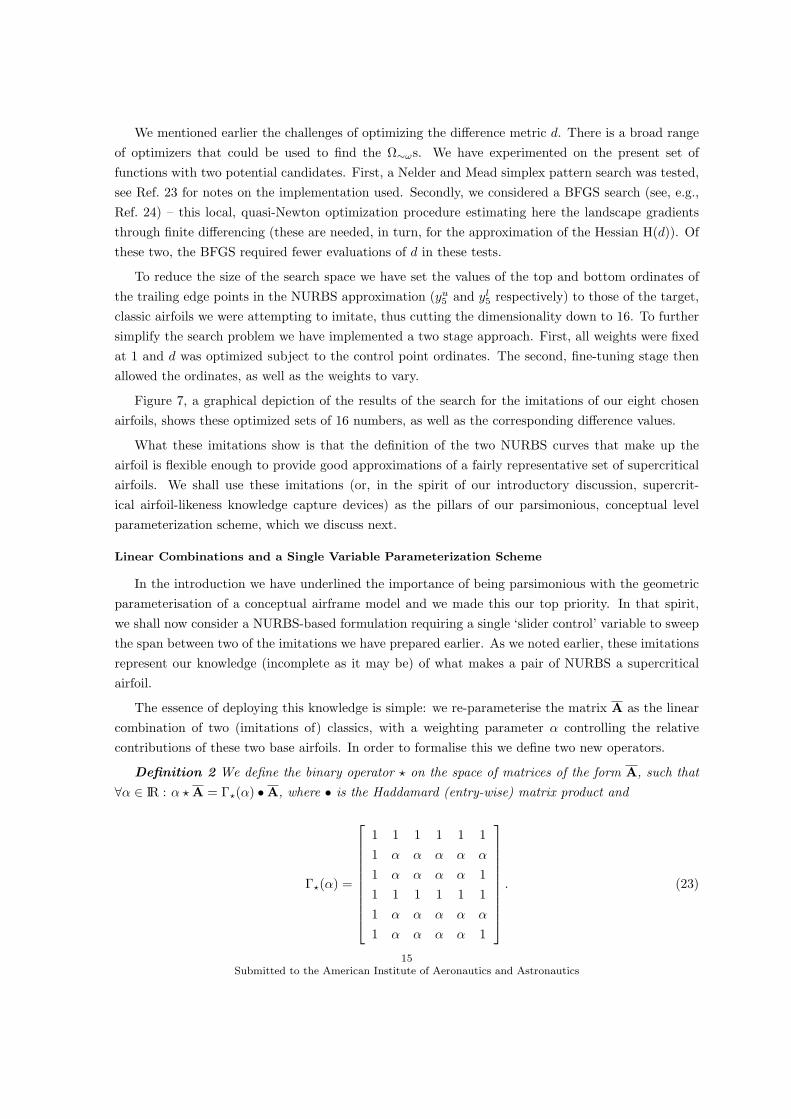
The essence of deploying this knowledge is simple: we re-parameterise the matrix A as the linearcombination of two (imitations of) classics, with a weighting parameter α controlling the relativecontributions of these two base airfoils. In order to formalise this we define two new operators.

Definition 2 We define the binary operator ? on the space of matrices of the form A, such that∀α ∈ IR : α ? A = Γ?(α) •A, where • is the Haddamard (entry-wise) matrix product and

Γ?(α) =

1 1 1 1 1 11 α α α α α

1 α α α α 11 1 1 1 1 11 α α α α α

1 α α α α 1

. (23)


Definition 3 We define the binary operator ⊕ on the space of matrices of the form A, such that∀A1,A2 : A1 ⊕A2 = A1 + Γ⊕ •A2, where • is the Haddamard (entry-wise) matrix product and

Γ⊕ =

0 0 0 0 0 00 1 1 1 1 10 1 1 1 1 00 0 0 0 0 00 1 1 1 1 10 1 1 1 1 0

. (24)

The matrices Γ?(α) and Γ⊕ are, essentially, stencils that control the elements of the genericparameterization that will be altered during the linear combination operation, which we define next.

Definition 4 Consider the NURBS imitations of some airfoils ω1 and ω2, denoted by Ωω1 =Ω(Aω1) and Ωω2 = Ω(Aω2) respectively (i.e., Aω1 and Aω2 contain the variables that define the twoimitations). We shall refer to the single-variable, parametric airfoil

Ωω2ω1(α) = Ω

[α ? Aω1 ⊕ (1− α) ? Aω2

],

where α ∈ [0, 1], as a linear combination NURBS airfoil over the bases ω1 and ω2.

The question arising now is, which bases ω1 and ω2 would ensure the best coverage of the designspace as α sweeps its range? We have the eight imitations of Section IV to choose from – the questionis, how do we measure the suitability of a given pair? As per criterion 4, for a given k we aim tomaximize the ability of the parametric airfoil to approximate existing supercritical sections. We canestimate this ability, using the overlapping areas once again as the difference metric in the same wayas we did with the imitations, by attempting to approximate a set of test sections, representative ofthe supercritical family. In addition to the eight potential base sections, we have also included inthis test set four more NASA phase 2 supercriticals for a better representation of the mid-range ofthickness to chord ratios: SC(2)-0410, SC(2)-0710, SC(2)-0412 and SC(2)-0712. We have evaluatedthe comparative abilities of the C2

8 = 28 possible basis pairs to represent the 12 airfoils in this set. Wehave found the ‘partnership’ of NLR7301 and SC(2)-0606 to work best. More formally, the evaluationof

min

12∑

i=1

minα

d[ωi,Ωωbase2

ωbase1(α)

]∣∣∣∣∣ (ωbase1, ωbase2) ⊂ B

(25)

resulted in (ωbase1, ωbase2)=(NLR7301, SC(2)-0606), where ω1 =SC(2)-0406, ω2 = SC(2)-0606, . . . ω12 =NLR7301 are the test airfoils (see the legend of Figure 8 for the full list) and

B = SC(2)− 0406, SC(2)− 0606, . . . NLR7301

is the list of the eight potential bases (as shown in Figure 7).

This is not a particularly surprising outcome, as one would intuitively expect the process to yieldone of the thinnest and one of the thickest airfoils as the best pillars, though it would have been


0 0.2 0.4 0.6 0.8 110

0

101

102

1−α

d

SC(2)−0406SC(2)−0606SC(2)−0706SC(2)−0410SC(2)−0710SC(2)−0412SC(2)−0712SC(2)−0714SC(2)−0518RAE2822RAE5215NLR7301min d (α)min d (α,w)min d (α,w,y)

Fig. 8 Plots of d[ωi, Ω

∼SC(2)−0606∼NLR7301 (α)

]for ω1 =SC(2)-0406, ω2 =SC(2)-0606,. . . ω12 =NLR7301.

The ‘+’ symbols indicate the minimum of each curve, i.e., the ordinates of these indicate the

minimum difference to within which the linear combination of NLR7301 and SC(2)-0606 can

approximate the 12 foils in our test set. The diamond symbols indicate the minimum difference

achievable through a local search started from that airfoil, which allows the control point weights

to vary, while the ordinates of the triangles indicate the minimum d achievable by also allowing

the control point ordinates to change during a single start local search.

harder to predict exactly which of the two thick and which of the three thin foils would provide thebest ‘supercritical airfoil-ness’ knowledge representation. Approximating the 12 members of the testset with linear combinations of the chosen pair gave an average minimum difference of

112

12∑

i=1

minα

d[ωi, Ω

∼SC(2)−0606∼NLR7301 (α)

]= 9.0601%. (26)

This experiment is captured graphically in Figure 8. The difference (d) curves corresponding toeach test airfoil can be seen dipping, for an optimum value of the linear combination factor α, to aminimum – this is the point where the parametric airfoil Ω∼SC(2)−0606

∼NLR7301 (α) resembles the target (test)airfoil most closely. For example,

Ω∼SC(2)−0606∼NLR7301 (0.675) = Ω

[0.675 ? A∼NLR7301 ⊕ 0.325 ? A∼SC(2)−0606

](27)

is the best approximation of SC(2)-0714 (d = 7.1993) that can be found using this scheme (we haverun a direct search over the α domain with a resolution of 10−2 here – the curves show that there islittle to be gained by employing a higher resolution search).


It is worth emphasizing once more that, in the spirit of our list of requirements postulated in theintroduction, we did not aim (and, indeed, cannot really hope) for extremely accurate approximationshere. Instead, we are exploring what is the best we can do with a single design variable available forcontrolling a parametric supercritical airfoil, while ensuring the satisfaction of the four other items ofour wish list from the beginning of Section V. On that note, let us now review the significance of theabove discussion from the conceptual design standpoint, which is at the centre of this paper.

Designing with Linear Combination NURBS Airfoils

Let v1, v2, . . . vk be a set of design variables that define an airframe geometry. As we are focusingon airfoil definition here, let v1 be the single parameter we are using to define, say, the wing rootsection. We do this as described above by building a control polygon and a pair of NURBS curves(as depicted in Figure 5), with the numbers needed to do this contained in the definition matrix,calculated in terms of the design variable v1 as

A = v1 ? A∼NLR7301 ⊕ (1− v1) ? A∼SC(2)−0606. (28)

For convenience we split the airframe description into the airfoil thus defined, Ω∼SC(2)−0606∼NLR7301 (v1),

and G(v2, v3, . . . vk), the latter denoting the rest of the geometry.

Consider now the functional F[Ω∼SC(2)−0606∼NLR7301 (v1), G(v2, v3, . . . vk)

]mapping some figure of merit

to the airframe geometry. Typically, this is an objective (computed through a numerical simulation),which we seek to maximize or minimize. An example is total airframe drag at the angle of attackwhere the total lift equals the all-up weight. Thus, the conceptual design search can be boiled downto the minimization problem

minv1∈[0,1],v2,...vk

F[Ω∼SC(2)−0606∼NLR7301 (v1), G(v2, v3, . . . vk)

], (29)

to whose dimensionality the airfoil only contributes one.

The linear combination NURBS airfoil essentially represents a continuum of supercritical airfoilsbetween the two bases, whose imitations it reproduces exactly at the extreme values of v1 (NLR7301at v1 = 0 and SC(2)-0606 at v1 = 1). Therefore, the optimization problem (29) can be solved withany continuous variable optimization algorithm. As an aside, the same geometric construction can beused for a search over a given catalog of imitations, rather than over the continuum bridging the gapbetween two imitations. For example, if we take the set B of our eight imitated classic airfoils (thoseshown in Figure 7) as the catalog, the problem can be re-cast as:

minv1∈1,2...,8,v2,...vk

F [Ω∼B(v1), G(v2, v3, . . . vk)

], (30)

which means that the search will now be discrete-valued along the dimension v1.

Returning now briefly to Figure 8, earlier we left unexplained part of the experiment depictedtherein and this is the appropriate moment to return to it. For every test airfoil, once we haveestablished the weighting that brings the parametric linear combination NURBS airfoil nearest to it,we froze the weighting at that value and further minimized the difference d using a Nelder and Mead


simplex pattern search, this time subject to the control point weights. The optima of these eight-dimensional local search processes can be read off the chart as the ordinates of the diamond symbols(note that these are not the globally best approximations that can be obtained for the various testairfoils, merely the minima of the local basins of attraction). Next, we ran the Nelder and Meadsearch once more, this time allowing both the weights and the control point ordinates to vary, givingthe minima whose difference values are the ordinates of the triangle symbols.

This logic could also be applied to the optimization of F at the later stages of the development pro-cess, perhaps as a preliminary design operation, where we are willing to trade increased dimensionalityfor potentially better objective functional value. Defining the stencil matrix

Γw =

0 0 0 0 0 00 0 0 0 0 00 1 1 1 1 00 0 0 0 0 00 0 0 0 0 00 1 1 1 1 0

, (31)

we can formalize this operation as

minΓw•A,v2,...vk

F[Ω∼SC(2)−0606∼NLR7301 (vopt

1 ), G(v2, v3, . . . vk)], (32)

where we have frozen v1 at vopt1 , the optimum value found during the conceptual design process and

we are now allowing the control point weights to be subjected to the optimization process. Finally,mirroring the experiments of Figure 8 in a real, design optimization context, we can now turn on allof the degrees of freedom built into our NURBS airfoil definition by allowing every entry in A to varyin an optimization process that can be summarized as:

minA,v2,...vk

F[Ω∼SC(2)−0606∼NLR7301 (vopt

1 ), G(v2, v3, . . . vk)]. (33)

At this level the formulation proposed here becomes very similar to those described by Lepine et al.6

and Painchaud-Ouellet et al.7 In terms of meeting our initial criteria listed at the beginning of SectionV, these last two preliminary design type steps now have increasing dimensionalities, which are hardto justify against criterion one. Also, they depart from the third criterion of our wish list, as theparameterisation can now yield ‘unphysical’ shapes too (although these are fairly unlikely to occur, asan aerodynamics-based F will probably still favor smooth, ‘reasonable’ shapes). We have, however,used the same geometrical entities for these different levels of optimization (criterion five), by merelyvarying the method whereby the control point weights and ordinates are calculated. In other words,the same model can be used throughout the entire design process, offering potential benefits in termsof development cost reduction.

Let us now return to the pure linear combination approach by considering the possibility of incor-porating additional knowledge into the parametric foil, simply by using additional learning cases.


Learning from More Examples

Let us consider the potential flexibility enhancements that additional base airfoils (as furtherlearning examples) would buy us. To this end, it is fairly straightforward to conceive an extension ofDefinition 4, as follows.

Definition 5 Consider the NURBS imitations of four airfoils ω1, ω2, ω3 and ω4, denoted byΩω1 = Ω(Aω1), Ωω2 = Ω(Aω2), Ωω3 = Ω(Aω3) and Ωω4 = Ω(Aω4) respectively (i.e., Aω1,Aω2,Aω3

and Aω4 contain the variables that define the four imitations). We shall refer to the parametric airfoil

ω1Ωω3ω2(α1, α2, α3) = Ω

[α1 ? Aω1 ⊕ α2 ? Aω2 ⊕ α3 ? Aω3

],

where α1, α2, α3 ∈ IR+ and α1 + α2 + α3 = 1, as a linear combination NURBS airfoil over the

bases ω1,ω2 and ω3 and to the parametric airfoil

ω4ω1Ω

ω3ω2(α1, α2, α3, α4) = Ω

[α1 ? Aω1 ⊕ α2 ? Aω2 ⊕ α3 ? Aω3 ⊕ α4 ? Aω4

],

where α1, α2, α3, α4 ∈ IR+ and α1 + α2 + α3 + α4 = 1, as a linear combination NURBS airfoil

over the bases ω1,ω2,ω3 and ω4.

The problem of approximating a given target airfoil with a linear combination NURBS airfoil overthree bases is virtually the same as with two bases. The only exception is that the optimization problemis now subject to three α’s instead of one. The overall dimensionality is reduced from three to twoby the additional equality constraint, though in most cases, from a computational implementationstandpoint, the problem is more readily viewed as three dimensional and constrained, rather thanprojected onto the two-dimensional plane α1 + α2 + α3 = 1 (α1, α2, α3 ∈ IR+) and unconstrained (seethe homomorphous mapping approach of Monson and Seppi25 for taking this latter route, if preferred).

Once again, we need to select the bases that, with their α’s optimized, best approximate the othermembers of our representative set of 12 test airfoils (this being a simple test of the satisfaction ofcriterion 4). Formally, we are seeking the solution of the two level minimization problem

min

12∑

i=1

minα1,α2,α3

d[ωi,ωbase1 Ωωbase3

ωbase2(α1, α2, α3)

]∣∣∣∣∣ (ωbase1, ωbase2, ωbase3) ⊂ B

,

where all C38 = 56 subsets of three of the set of eight potential base airfoils are tested across the set

of 12 test airfoils. A direct search solve of (34) yielded

(ωbase1, ωbase2, ωbase3) = (RAE5215, SC(2)− 0518, SC(2)− 0606),

with the difference metric averaging 7.0315% over the 12 target sections, which is around three quartersof the estimated average approximation error of the two basis airfoil scheme (9.0601%). To single outone particular example, the difference metric between SC(2)-0714 and its best approximation was


ω α1 α2 α3 d[ω, ∼RAE5215Ω

∼SC(2)−0606∼SC(2)−0518(α1, α2, α3)

]

SC(2)-0406 0.0042 0 0.9958 12.3886 %SC(2)-0606 0 0 1 4.1986 %SC(2)-0706 0 0 1 11.3089 %SC(2)-0410 0 0.2669 0.7331 9.1881 %SC(2)-0710 0.7072 0.0930 0.1997 10.7707 %SC(2)-0412 0 0.4496 0.5504 6.7767 %SC(2)-0712 0.6030 0.3121 0.0849 8.0071%SC(2)-0714 0.1237 0.5962 0.2801 4.6457 %SC(2)-0518 0 1 0 2.6060 %RAE2822 0.5172 0.3002 0.1826 7.5347 %RAE5215 1 0 0 0.9235 %NLR7301 0.2155 0.7845 0 6.0293 %

Table 1 The differences between the test set of twelve airfoils and the closest linear combination

NURBS airfoils over the bases RAE5215, SC(2)-0518 and SC(2)-0606, obtained by minimizing

d subject to α1,α2 and α3 (where α1 + α2 + α3 = 1).

found to be

d[SC(2)− 0714, ∼RAE5215Ω

∼SC(2)−0606∼SC(2)−0518(0.1237, 0.5962, 0.2801)

]=

= d[SC(2)− 0714, Ω

(0.1237 ? A∼RAE5215 ⊕ 0.5962 ? A∼SC(2)−0518 ⊕ 0.2801 ? A∼SC(2)−0606

)]=

= 4.6457%,

approximately two thirds of the difference metric value of the two basis approximation of SC(2)-0714(see equation (27)). Table 1 contains the full results of this experiment. Repeating now the exercisefor four bases, we seek the solution of the two level minimization problem

min

12∑

i=1

minα1,α2,α3,α4

d[ωi,

ωbase4ωbase1

Ωωbase3ωbase2

(α1, α2, α3, α4)]∣∣∣∣∣ (ωbase1, ωbase2, ωbase3, ωbase4) ⊂ B

,

where now the C48 = 70 subsets of four of the set of eight potential base airfoils are evaluated as

potential bases over the set of 12 test airfoils. From a direct search solve of (34) results

(ωbase1, ωbase2, ωbase3, ωbase4) = (RAE5215, SC(2)− 0518, SC(2)− 0706), SC(2)− 0406),

with the averaged difference metric now dropping to 4.9874% – comparing this to the best we couldachieve with only two basis airfoils (just under twice this difference metric value, 9.0601%) confirmsthe increase in the amount of additional geometrical features incorporated into the ‘knowledge base’of the parametric airfoil.

VI. Conclusions and Possible Extensions

We have presented four parametric airfoils, which, in our opinion, are suitable for conceptual designpurposes, on account of their low dimensionality. First we have looked at three simple schemes defined


ω α1 α2 α3 α4 d[ω,

∼SC(2)−0406∼RAE5215 Ω∼SC(2)−0706

∼SC(2)−0518(α1, α2, α3, α4)]

SC(2)-0406 0 0 0 1 2.1088 %SC(2)-0606 0 0 0.8886 0.1114 5.8129 %SC(2)-0706 0 0 1 0 5.8156 %SC(2)-0410 0 0.2968 0.1673 0.5359 4.0453 %SC(2)-0710 0.6250 0.1250 0.1250 0.1250 10.5663 %SC(2)-0412 0 0.4691 0.1431 0.3877 3.5596 %SC(2)-0712 0.5464 0.3378 0.0032 0.1124 7.9753 %SC(2)-0714 0.0245 0.6323 0.1302 0.2130 3.8678 %SC(2)-0518 0 1 0 0 2.6060 %RAE2822 0.4240 0.3417 0.0964 0.1380 6.8773 %RAE5215 1 0 0 0 0.9235 %NLR7301 0.2155 0.7845 0 0 6.0055 %

Table 2 The differences between the test set of twelve airfoils and the closest linear combination

NURBS airfoils over the bases RAE5215, SC(2)-0518, SC(2)-0706 and SC(2)-0406 obtained by

minimizing d subject to α1,α2,α3 and α4 (where α1 + α2 + α3 + α4 = 1).

by six variables each, which, while being easy to implement, are also sufficiently flexible to cover arange of ‘classic’ airfoils.

We then put forward a NURBS-based parametric airfoil specifically conceived for situations whenminimizing the number of design variables is the overwhelming driver and the target application istransonic wings. We began by looking at the absolute limit of conciseness: a single variable for-mulation. This parametric airfoil is a linear combination of two, carefully selected, well-establishedsupercritical shapes – the sole variable controls the relative contributions of these two basis sectionsto the parameterised shape. Clearly, the flexibility of this airfoil description is limited, but, as it canproduce a range of airfoils of different thickness to chord ratios, it allows, for example, one of thefundamental types of MDO study at the conceptual design level: the investigation of the optimumtrade-off between spar thickness, fuel tank capacity (assuming that the fuel is carried inside the wing)and drag.

More refined studies across a broader design space are possible using additional bases – we haveshown that adding one or two additional basis sections into the linear combination increases theflexibility (and thus design space coverage) of the parametric airfoil. Further, we have demonstrated,that the same geometrical setup used in the linear combination scheme can be ‘recycled’ for preliminarydesign studies, where, if we sacrifice parsimony, extra flexibility is available for local optimizationpurposes, without the need for re-building the model.

The general thrust of the approach described here can be adapted for other types of geometry,including NURBS surfaces. For instance, it would be possible to fit a NURBS surface to existingairliner fuselage shapes (maintaining the same control point arrangement) and use the linear com-bination approach to populate the design space defined by these basis fuselages. We envisage this


type of approach being particularly suited to the concise parameterisation of very complex shapes,as it is a simple way of reducing dimensionality using case-based knowledge about what constitutes a‘reasonable’ shape.

Acknowledgements

We would like to thank the Royal Academy of Engineering and the Engineering and PhysicalSciences Research Council (EPSRC) for the financial support of the first author’s work.

References1Jameson, A., “Aerodynamic Design via Control Theory,” Journal of Scientific Computing, Vol. 3, No. 3, 1988,

pp. 233–260.

2Jameson, A., “Optimum aerodynamic design using control theory,” in Hafez, M. and Oshima, K.(eds), Compu-

tational Fluid Dynamics Review, John Wiley & Sons, 1995.

3Hicks, R. M. and Henne, P. A., “Wing Design by Numerical Optimization,” Journal of Aircraft , Vol. 15, 1978,

pp. 407–412.

4Reuther, J., Jameson, A., Alonso, J. J., Remlinger, M. J., and Saunders, D., “Constrained Multipoint Aerody-

namic Shape Optimization using an Adjoint Formulation and Parallel Computers,” Journal of Aircraft , Vol. 36, No. 1,

1999, pp. 61–74.

5Kulfan, B. M., “Universal Parametric Geometry Representation Method,” Journal of Aircraft , Vol. 45, No. 1,

2008, pp. 142–158.

6Lepine, J., Guibault, F., J-Y., T., and Pepin, F., “Optimized Nonuniform Rational B-Spline Geometrical Repre-

sentation for Aerodynamic Design of Wings,” AIAA Journal , Vol. 39, No. 11, 2001, pp. 2033–2041.

7Painchaud-Ouellet, S., Tribes, C., Trepanier, J.-Y., and Pelletier, D., “Airfoil Shape Optimization Using a

Nonuniform Rational B-Splines Parameterization Under Thickness Constraint,” AIAA Journal , Vol. 44, No. 10, 2006,

pp. 2170–2178.

8Sobieczky, H., “Parametric Airfoils and Wings,” Notes on Numerical Fluid Mechanics, Fuji, K. and Dulikravich,

G. S. (Eds.), Vol. 68, 1998, pp. 71–88.

9Robinson, G. M. and Keane, A. J., “Concise Orthogonal Representation of Supercritical Airfoils,” Journal of

Aircraft , Vol. 38, No. 3, 2001.

10Harris, C. D., “NASA Supercritical Airfoils; A Matrix of Family-Related Airfoils,” Technical Paper 2969, NASA,

1990.

11Ferguson, J., “Multivariable Curve Interpolation,” Journal of the Association for Computing Machinery, Vol. 11,

No. 2, 1964, pp. 221–228.

12Sobester, A. and Keane, A., “Airfoil Design via Cubic Splines – Ferguson’s Curves Revisited,” AIAA-2007-2881 ,

2007.

13Cox, M. G., “The Numerical Evaluation of B-splines,” Journal of the Institute of Mathematics and its Applica-

tions, Vol. 10, 1972, pp. 134–149.

14De Boor, C., “On Calculating with B-splines,” Journal of Approximation Theory, Vol. 6, 1972, pp. 50–62.

15Piegl, L. and Tiller, W., The NURBS Book , Springer-Verlag, Heidelberg, 1997.

16Versprille, K. J., Computer-Aided Design Applications of the Rational B-spline Approximation Form, Ph.D.

thesis, Syracuse University, 1975.

17Schramm, U., Pilkey, W. D., DeVries, R. I., and Zebrowski, M. P., “Shape Design for Thin-Walled Beam Cross

Sections Using Rational B-Splines,” AIAA Journal , Vol. 33, No. 11, 1995, pp. 2205–2211.

18Samareh, J. A., “Novel Multidisciplinary Shape Parameterization Approach,” Journal of Aircraft , Vol. 38, No. 6,

2001, pp. 1015–1024.


19Jenkins, R. V., Hill, A. S., and Ray, E. J., “Aerodynamic performance and pressure distributions for a NASA

SC(2)-0714 airfoil tested in the Langley 0.3-meter transonic cryogenic tunnel,” Technical Memorandum NASA-TM-4044,

NASA Langley Research Center, 1988.

20Boerstoel, J. W. and Huizing, G. H., “Transonic Shock-Free Aerofoil Design by an Analytic Hodograph Method,”

Journal of Aircraft , Vol. 12, No. 9, 1975, pp. 730–736.

21“Experimental Data Base for Computer Program Assessment – Report of the Fluid Dynamics Panel Working

Group 04,” Advisory Report AR-138, AGARD, 1979.

22Wilby, P. G., “The Design and Aerodynamic Characteristics of the RAE 5215 Aerofoil,” Current Paper 1386,

Procurement Executive, Ministry of Defence, Aeronautical Research Council, 1974.

23Lagarias, J., Reeds, J. A., Wright, M. H., and Wright, P. E., “Convergence Properties of the Nelder-Mead Simplex

Method in Low Dimensions,” SIAM Journal of Optimization, Vol. 9, No. 1, 1998, pp. 112–147.

24Broyden, C. G., “The Convergence of a Class of Double-Rank Minimization Algorithms,” Journal of the Institute

of Mathematics and its Applications, Vol. 6, 1970, pp. 76–90.

25Monson, C. K. and Seppi, K. D., “Linear Equality Constraints and Homomorphous Mappings in PSO,” Proceed-

ings of the Congress on Evolutionary Computation, 2005, pp. 73–80.


the quest for a truly parsimonious airfoil ...eprints.soton.ac.uk/64913/1/sobe_08a.pdf · the quest...

Documents