the quarterly journal of economicsklenow.com/mmtfp.pdf · the quarterly journal of economics vol....

THE

QUARTERLY JOURNALOF ECONOMICS

Vol. CXXIV November 2009 Issue 4

MISALLOCATION AND MANUFACTURING TFPIN CHINA AND INDIA∗

CHANG-TAI HSIEH AND PETER J. KLENOW

Resource misallocation can lower aggregate total factor productivity (TFP). Weuse microdata on manufacturing establishments to quantify the potential extentof misallocation in China and India versus the United States. We measure sizablegaps in marginal products of labor and capital across plants within narrowlydefined industries in China and India compared with the United States. Whencapital and labor are hypothetically reallocated to equalize marginal products tothe extent observed in the United States, we calculate manufacturing TFP gainsof 30%–50% in China and 40%–60% in India.

I. INTRODUCTION

Large differences in output per worker between rich andpoor countries have been attributed, in no small part, to differ-ences in total factor productivity (TFP).1 The natural questionthen is: What are the underlying causes of these large TFP dif-ferences? Research on this question has largely focused on dif-ferences in technology within representative firms. For example,Howitt (2000) and Klenow and Rodrıguez-Clare (2005) show howlarge TFP differences can emerge in a world with slow technology

∗We are indebted to Ryoji Hiraguchi and Romans Pancs for phenomenalresearch assistance, and to seminar participants, referees, and the editors forcomments. We gratefully acknowledge the financial support of the Kauffman Foun-dation. Hsieh thanks the Alfred P. Sloan Foundation and Klenow thanks SIEPRfor financial support. The research in this paper on U.S. manufacturing was con-ducted while the authors were Special Sworn Status researchers of the U.S. CensusBureau at the California Census Research Data Center at UC Berkeley. Researchresults and conclusions expressed are those of the authors and do not necessarilyreflect the views of the Census Bureau. This paper has been screened to ensurethat no confidential data are revealed. [email protected], [email protected].

1. See Caselli (2005), Hall and Jones (1999), and Klenow and Rodrıguez-Clare(1997).

C© 2009 by the President and Fellows of Harvard College and the Massachusetts Institute ofTechnology.The Quarterly Journal of Economics, November 2009

1403

1404 QUARTERLY JOURNAL OF ECONOMICS

diffusion from advanced countries to other countries. These aremodels of within-firm inefficiency, with the inefficiency varyingacross countries.

A recent paper by Restuccia and Rogerson (2008) takes a dif-ferent approach. Instead of focusing on the efficiency of a repre-sentative firm, they suggest that misallocation of resources acrossfirms can have important effects on aggregate TFP. For example,imagine an economy with two firms that have identical technolo-gies but in which the firm with political connections benefits fromsubsidized credit (say from a state-owned bank) and the other firm(without political connections) can only borrow at high interestrates from informal financial markets. Assuming that both firmsequate the marginal product of capital with the interest rate, themarginal product of capital of the firm with access to subsidizedcredit will be lower than the marginal product of the firm that onlyhas access to informal financial markets. This is a clear case ofcapital misallocation: aggregate output would be higher if capitalwas reallocated from the firm with a low marginal product to thefirm with a high marginal product. The misallocation of capitalresults in low aggregate output per worker and TFP.

Many institutions and policies can potentially result in re-source misallocation. For example, the McKinsey Global Institute(1998) argues that a key factor behind low productivity in Brazil’sretail sector is labor-market regulations driving up the cost of la-bor for supermarkets relative to informal retailers. Despite theirlow productivity, the lower cost of labor faced by informal-sectorretailers makes it possible for them to command a large share ofthe Brazilian retail sector. Lewis (2004) describes many similarcase studies from the McKinsey Global Institute.

Our goal in this paper is to provide quantitative evidence onthe potential impact of resource misallocation on aggregate TFP.We use a standard model of monopolistic competition with het-erogeneous firms, essentially Melitz (2003) without internationaltrade, to show how distortions that drive wedges between themarginal products of capital and labor across firms will lower ag-gregate TFP.2 A key result we exploit is that revenue productivity(the product of physical productivity and a firm’s output price)should be equated across firms in the absence of distortions. Tothe extent revenue productivity differs across firms, we can use itto recover a measure of firm-level distortions.

2. In terms of the resulting size distribution, the model is a cousin to theLucas (1978) span-of-control model.

MISALLOCATION AND TFP IN CHINA AND INDIA 1405

We use this framework to measure the contribution of re-source misallocation to aggregate manufacturing productivity inChina and India versus the United States. China and India areof particular interest not only because of their size and rela-tive poverty, but because they have carried out reforms that mayhave contributed to their rapid growth in recent years.3 We useplant-level data from the Chinese Industrial Survey (1998–2005),the Indian Annual Survey of Industries (ASI; 1987–1994), and theU.S. Census of Manufacturing (1977, 1982, 1987, 1992, and 1997)to measure dispersion in the marginal products of capital andlabor within individual four-digit manufacturing sectors in eachcountry. We then measure how much aggregate manufacturingoutput in China and India could increase if capital and labor werereallocated to equalize marginal products across plants withineach four-digit sector to the extent observed in the United States.The United States is a critical benchmark for us, because theremay be measurement error and factors omitted from the model(such as adjustment costs and markup variation) that generategaps in marginal products even in a comparatively undistortedcountry such as the United States.

We find that moving to “U.S. efficiency” would increase TFPby 30%–50% in China and 40%–60% in India. The output gainswould be roughly twice as large if capital accumulated in re-sponse to aggregate TFP gains. We find that deteriorating alloca-tive efficiency may have shaved 2% off Indian manufacturing TFPgrowth from 1987 to 1994, whereas China may have boosted itsTFP 2% per year over 1998–2005 by winnowing its distortions. Inboth India and China, larger plants within industries appear tohave higher marginal products, suggesting they should expand atthe expense of smaller plants. The pattern is much weaker in theUnited States.

Although Restuccia and Rogerson (2008) is the closest prede-cessor to our investigation in model and method, there are manyothers.4 In addition to Restuccia and Rogerson, we build on three

3. For discussion of Chinese reforms, see Young (2000, 2003) and TheEconomist (2006b). For Indian reforms, see Kochar et al. (2006), The Economist(2006a), and Aghion et al. (2008). Dobson and Kashyap (2006), Farrell and Lund(2006), Allen et al. (2007), and Dollar and Wei (2007) discuss how capital continuesto be misallocated in China and India.

4. A number of other authors have focused on specific mechanisms that couldresult in resource misallocation. Hopenhayn and Rogerson (1993) studied the im-pact of labor market regulations on allocative efficiency; Lagos (2006) is a recenteffort in this vein. Caselli and Gennaioli (2003) and Buera and Shin (2008) modelinefficiencies in the allocation of capital to managerial talent, while Guner, Ven-tura, and Xu (2008) model misallocation due to size restrictions. Parente and


papers in particular. First, we follow the lead of Chari, Kehoe,and McGrattan (2007) in inferring distortions from the residu-als in first-order conditions. Second, the distinction between afirm’s physical productivity and its revenue productivity, high-lighted by Foster, Haltiwanger, and Syverson (2008), is centralto our estimates of resource misallocation. Third, Banerjee andDuflo (2005) emphasize the importance of resource misallocationin understanding aggregate TFP differences across countries, andpresent suggestive evidence that gaps in marginal products of cap-ital in India could play a large role in India’s low manufacturingTFP relative to that of the United States.5

The rest of the paper proceeds as follows. We sketch a modelof monopolistic competition with heterogeneous firms to show howthe misallocation of capital and labor can lower aggregate TFP.We then take this model to the Chinese, Indian, and U.S. plantdata to try to quantify the drag on productivity in China and Indiadue to misallocation in manufacturing. We lay out the model inSection II, describe the data sets in Section III, and present po-tential gains from better allocation in Section IV. In Section V wetry to assess whether greater measurement error in China andIndia could explain away our results. In Section VI we make afirst pass at relating observable policies to allocative efficiency inChina and India. In Section VII we explore alternative explana-tions besides policy distortions and measurement error. We offersome conclusions in Section VIII.

II. MISALLOCATION AND TFP

This section sketches a standard model of monopolistic com-petition with heterogeneous firms to illustrate the effect of re-source misallocation on aggregate productivity. In addition todiffering in their efficiency levels (as in Melitz [2003]), we assumethat firms potentially face different output and capital distortions.

We assume there is a single final good Y produced by a repre-sentative firm in a perfectly competitive final output market. Thisfirm combines the output Ys of S manufacturing industries using

Prescott (2000) theorize that low-TFP countries are ones in which vested interestsblock firms from introducing better technologies.

5. See Bergoeing et al. (2002), Galindo, Schiantarelli, and Weiss (2007), Alfaro,Charlton, and Kanczuk (2008), and Bartelsman, Haltiwanger, and Scarpetta(2008) for related empirical evidence in other countries.


a Cobb-Douglas production technology:

(1) Y =S∏

s=1

Y θss , where

S∑s=1

θs = 1.

Cost minimization implies

(2) PsYs = θs PY.

Here, Ps refers to the price of industry output YS and P ≡∏Ss = 1 (Ps/θs)θs represents the price of the final good (the final good

is our numeraire, and so P = 1). Industry output Ys is itself a CESaggregate of Ms differentiated products:

(3) Ys =(

Ms∑i=1

Yσ−1

σ

si

) σσ−1

.

The production function for each differentiated product is givenby a Cobb-Douglas function of firm TFP, capital, and labor:

(4) Ysi = Asi Kαssi L1−αs

si .

Note that capital and labor shares are allowed to differ acrossindustries (but not across firms within an industry).6

Because there are two factors of production, we can sepa-rately identify distortions that affect both capital and labor fromdistortions that change the marginal product of one of the factorsrelative to the other factor of production. We denote distortionsthat increase the marginal products of capital and labor by thesame proportion as an output distortion τY . For example, τY wouldbe high for firms that face government restrictions on size or hightransportation costs, and low in firms that benefit from publicoutput subsidies. In turn, we denote distortions that raise themarginal product of capital relative to labor as the capital distor-tion τK. For example, τK would be high for firms that do not haveaccess to credit, but low for firms with access to cheap credit (bybusiness groups or state-owned banks).

Profits are given by

(5) πsi = (1 − τY si)PsiYsi − wLsi − (1 + τKsi)RKsi.

6. In Section VII (“Alternative Explanations”), we relax this assumption byreplacing the plant-specific capital distortion with plant-specific factor shares.


Note that we assume all firms face the same wage, an issue towhich we return later. Profit maximization yields the standardcondition that the firm’s output price is a fixed markup over itsmarginal cost:

(6) Psi = σ

σ − 1

(Rαs

)αs(

w

1 − αs

)1−αs (1 + τKsi)αs

Asi (1 − τY si).

The capital-labor ratio, labor allocation, and output are given by

Ksi

Lsi= αs

1 − αs· w

R· 1

(1 + τKsi),(7)

Lsi ∝ Aσ−1si (1 − τY si)σ

(1 + τKsi)αs(σ−1),(8)

Ysi ∝ Aσsi(1 − τY si)σ

(1 + τKsi)αs σ.(9)

The allocation of resources across firms depends not only on firmTFP levels, but also on the output and capital distortions theyface. To the extent resource allocation is driven by distortionsrather than firm TFP, this will result in differences in the marginalrevenue products of labor and capital across firms. The marginalrevenue product of labor is proportional to revenue per worker:

(10) MRPLsi�= (1 − αS)

σ − 1σ

PsiYsi

Lsi= w

11 − τY si

.

The marginal revenue product of capital is proportional to therevenue-capital ratio:

(11) MRPKsi�= αS

σ − 1σ

PsiYsi

Ksi= R

1 + τKsi

1 − τY si.

Intuitively, the after-tax marginal revenue products of capital andlabor are equalized across firms. The before-tax marginal revenueproducts must be higher in firms that face disincentives, and canbe lower in firms that benefit from subsidies.

We are now ready to derive an expression for aggregate TFPas a function of the misallocation of capital and labor. We first


solve for the equilibrium allocation of resources across sectors:7

Ls ≡Ms∑i=1

Lsi = L(1 − αs) θs/MRPLs∑S

s′=1 (1 − αs′ ) θs′/MRPLs′,(12)

Ks ≡Ms∑i=1

Ksi = Kαs θs/MRPKs∑S

s′=1 αs′ θs′/MRPKs′.(13)

Here,

MRPLs ∝(

Ms∑i=1

11 − τY si

PsiYsi

PsYs

),

MRPKs ∝(

Ms∑i=1

1 + τKsi

1 − τY si

PsiYsi

PsYs

)

denote the weighted average of the value of the marginal productof labor and capital in a sector, and L ≡ ∑S

s=1 Ls and K ≡ ∑Ss=1 Ks

represent the aggregate supply of labor and capital. We can thenexpress aggregate output as a function of KS, LS, and industryTFP:8

(14) Y =S∏

s=1

(TFPs · Kαs

s · L1−αss

)θs.

To determine the formula for industry productivity TFPs, it is use-ful to show that firm-specific distortions can be measured by thefirm’s revenue productivity. It is typical in the productivity liter-ature to have industry deflators but not plant-specific deflators.Foster, Haltiwanger, and Syverson (2008) stress that, when indus-try deflators are used, differences in plant-specific prices show upin the customary measure of plant TFP. They stress the distinc-tion between “physical productivity,” which they denote TFPQ,and “revenue productivity,” which they call TFPR. The use of aplant-specific deflator yields TFPQ, whereas using an industrydeflator gives TFPR.

7. To derive Ks and Ls we proceed as follows: First, we derive the aggregatedemand for capital and labor in a sector by aggregating the firm-level demandsfor the two factor inputs. We then combine the aggregate demand for the factorinputs in each sector with the allocation of total expenditure across sectors.

8. We combine the aggregate demand for capital and labor in a sector, theexpression for the price of aggregate industry output, and the expression for theprice of aggregate output.


The distinction between physical and revenue productivity isvital for us too. We define these objects as follows:9

TFPQsi�= Asi = Ysi

Kαssi (wLsi)1−αs

TFPRsi�= Psi Asi = PsiYsi

Kαssi (wLsi)1−αs

.

In our simple model, TFPR does not vary across plants withinan industry unless plants face capital and/or output distortions.In the absence of distortions, more capital and labor should beallocated to plants with higher TFPQ to the point where theirhigher output results in a lower price and the exact same TFPR asat smaller plants. Using (10) and (11), plant TFPR is proportionalto a geometric average of the plant’s marginal revenue productsof capital and labor:10

TFPRsi ∝ (MRPKsi)αs (MRPLsi)

1−αs ∝ (1 + τKsi)αs

1 − τY si.

High plant TFPR is a sign that the plant confronts barriers thatraise the plant’s marginal products of capital and labor, renderingthe plant smaller than optimal.

With the expression for TFPR in hand, we can express indus-try TFP as

(15) TFPs =⎡⎣ Ms∑

i=1

(Asi · TFPRs

TFPRsi

)σ−1⎤⎦

1σ−1

,

where TFPRs ∝ (MRPKs)αs (MRPLs)1−αs is a geometric average ofthe average marginal revenue product of capital and labor in thesector.11 If marginal products were equalized across plants, TFPwould be As = (

∑Msi=1 Aσ−1

si )1

σ−1 . Equation (15) is the key equation weuse for our empirical estimates. Appendix I shows that we wouldarrive at an expression similar to (15) if we assumed a Lucasspan-of-control model rather than monopolistic competition.

9. To crudely control for differences in human capital we measure labor inputas the wage bill, which we denote as the product of a common wage per unit ofhuman capital w and effective labor input Lsi .

10. TFPRsi = σσ−1

(MRPKsi

αS

)αs (MRPLsiw (1−αS)

)1−αs =(

RαS

)αs (1

1−αS

)1−αs (1+τKsi )αs

1−τYsi.

11. TFPRs =[

RαS

∑Msi=1

(1+τKsi1−τYsi

)·(

PsiYsiPsYs

)]αs [1

1−αS

∑Msi=1

(1

1−τYsi

)(PsiYsiPsYs

)]1−αs.


When A (≡ TFPQ) and TFPR are jointly lognormally dis-tributed, there is a simple closed-form expression for aggregateTFP:

(16) log TFPs = 1σ − 1

log

(Ms∑i=1

Aσ−1si

)− σ

2var (log TFPRsi) .

In this special case, the negative effect of distortions on aggregateTFP can be summarized by the variance of log TFPR. Intuitively,the extent of misallocation is worse when there is greater disper-sion of marginal products.

We note several things about the effect of misallocation onaggregate TFP in this model. First, from (12) and (13), the sharesof aggregate labor and capital in each sector are unaffected by theextent of misallocation as long as average marginal revenue prod-ucts are unchanged. Our Cobb-Douglas aggregator (unit elasticdemand) is responsible for this property (an industry that is 1%more efficient has a 1% lower price index and 1% higher demand,which can be accommodated without adding or shedding inputs).We later relax the Cobb-Douglas assumption to see how much itmatters.

Second, we have conditioned on a fixed aggregate stock ofcapital. Because the rental rate rises with aggregate TFP, wewould expect capital to respond to aggregate TFP (even with afixed saving and investment rate). If we endogenize K by invokinga consumption Euler equation to pin down the long-run rentalrate R, the output elasticity with respect to aggregate TFP is1/(1 − ∑S

s=1 αSθS). Thus the effect of misallocation on output isincreasing in the average capital share. This property is reminis-cent of a one-sector neoclassical growth model, wherein increasesin TFP are amplified by capital accumulation so that the outputelasticity with respect to TFP is 1/(1 − α).

Third, we assume that the number of firms in each industryis not affected by the extent of misallocation. In an Appendixavailable upon request, we show that the number of firms would beunaffected by the extent of misallocation in a model of endogenousentry in which entry costs take the form of a fixed amount oflabor.12

12. We assume entrants do not know their productivity or distortions beforeexpending entry costs, only the joint distribution of distortions and productivityfrom which they will draw. We also follow Melitz (2003) and Restuccia and Roger-son (2008) in assuming exogenous exit among producers. Unlike Melitz, however,


III. DATA SETS FOR INDIA, CHINA, AND THE UNITED STATES

Our data for India are drawn from India’s ASI conductedby the Indian government’s Central Statistical Organisation. TheASI is a census of all registered manufacturing plants in Indiawith more than fifty workers (one hundred if without power) anda random one-third sample of registered plants with more thanten workers (twenty if without power) but less than fifty (or onehundred) workers. For all calculations we apply a sampling weightso that our weighted sample reflects the population. The surveyprovides information on plant characteristics over the fiscal year(April of a given year through March of the following year). Weuse the ASI data from the 1987–1988 through 1994–1995 fiscalyears. The raw data consist of around 40,000 plants in each year.

The variables in the ASI that we use are the plant’s industry(four-digit ISIC), labor compensation, value-added, age (based onreported birth year), and book value of the fixed capital stock.Specifically, the ASI reports the plant’s total wage payments,bonus payments, and the imputed value of benefits. Our measureof labor compensation is the sum of wages, bonuses, and benefits.In addition, the ASI reports the book value of fixed capital at thebeginning and end of the fiscal year net of depreciation. We takethe average of the net book value of fixed capital at the beginningand end of the fiscal year as our measure of the plant’s capital. Wealso have ownership information from the ASI, although the own-ership classification does not distinguish between foreign-ownedand domestic plants.

Our data for Chinese firms (not plants) are from Annual Sur-veys of Industrial Production from 1998 through 2005 conductedby the Chinese government’s National Bureau of Statistics. TheAnnual Survey of Industrial Production is a census of all nonstatefirms with more than 5 million yuan in revenue (about $600,000)plus all state-owned firms. The raw data consist of over 100,000firms in 1998 and grow to over 200,000 firms in 2005. Hereafterwe often refer to Chinese firms as “plants.”

The information we use from the Chinese data are the plant’sindustry (again at the four-digit level), age (again based on

we do not have overhead costs. Because of the overhead costs in Melitz, somefirms exit after spending entry costs but before commencing production, therebycreating an endogenous form of exit that truncates the left tail of the productivitydistribution. We leave it as an important topic for future research to investigate theimpact of distortions on aggregate productivity and welfare through endogenousentry and exit.


reported birth year), ownership, wage payments, value-added, ex-port revenues, and capital stock. We define the capital stock as thebook value of fixed capital net of depreciation. As for labor com-pensation, the Chinese data only report wage payments; they donot provide information on nonwage compensation. The medianlabor share in plant-level data is roughly 30%, which is signif-icantly lower than the aggregate labor share in manufacturingreported in the Chinese input-output tables and the national ac-counts (roughly 50%). We therefore assume that nonwage benefitsare a constant fraction of a plant’s wage compensation, where theadjustment factor is calculated such that the sum of imputed ben-efits and wages across all plants equals 50% of aggregate value-added. We also have ownership status for the Chinese plants.Chinese manufacturing had been predominantly state run or stateinvolved, but was principally private by the end of our sample.13

Our main source for U.S. data is the Census of Manufactures(CM) from 1977, 1982, 1987, 1992, and 1997 conducted by theU.S. Bureau of the Census. Befitting its name, the census cov-ers all manufacturing plants. We drop small plants with limitedproduction data (Administrative Records), leaving over 160,000plants in each year. The information we use from the U.S. Cen-sus are the plant’s industry (again at the four-digit level), laborcompensation (wages and benefits), value-added, export revenues,and capital stock. We define the capital stock as the average ofthe book value of the plant’s machinery and equipment and struc-tures at the beginning and at the end of the year. The U.S. data donot provide information on plant age. We impute the plant’s ageby determining when the plant appears in the data for the firsttime.14

For our computations we set industry capital shares to thosein the corresponding U.S. manufacturing industry. As a result, wedrop nonmanufacturing plants and plants in industries withouta close counterpart in the United States. We also trim the 1%tails of plant productivity and distortions in each country-year tomake the results robust to outliers. Later we check robustness toadjusting the book values of capital for inflation.

13. Our data may understate the extent of privatization. Dollar and Wei (2007)conducted their own survey of Chinese firms in 2005 and found that 15% of allfirms were officially classified as state owned but had in fact been privatized.

14. For plants in the Annual Survey of Manufactures (ASM), we use theannual data of the ASM (starting with the 1963 ASM) to identify the plant’s birthyear. For the plants that are not in the ASM, we assume the birth year is the yearthe plant first appears in the quinquennial CM minus three years.


IV. POTENTIAL GAINS FROM REALLOCATION

To calculate the effects of resource misallocation, we need toback out key parameters (industry output shares, industry cap-ital shares, and the firm-specific distortions) from the data. Weproceed as follows:

We set the rental price of capital (excluding distortions) toR = 0.10. We have in mind a 5% real interest rate and a 5%depreciation rate. The actual cost of capital faced by plant i inindustry s is denoted (1 + τKsi)R, and so it differs from 10% if τKsi �=0. Because our hypothetical reforms collapse τKsi to its average ineach industry, the attendant efficiency gains do not depend on R.If we have set R incorrectly, it affects only the average capitaldistortion, not the liberalization experiment.

We set the elasticity of substitution between plant value-added to σ = 3. The gains from liberalization are increasing inσ , as is explicit in (16), and so we made this choice conserva-tively. Estimates of the substitutability of competing manufac-tures in the trade and industrial organization literatures typicallyrange from three to ten (e. g., Broda and Weinstein [2006], Hendeland Nevo [2006]). Later we entertain the higher value of 5 forσ as a robustness check. Of course, the elasticity surely differsacross goods (Broda and Weinstein report lower elasticities formore differentiated goods), so our single σ is a strong simplifyingassumption.

As mentioned, we set the elasticity of output with respect tocapital in each industry (αs) to be 1 minus the labor share in thecorresponding industry in the United States. We do not set theseelasticities on the basis of labor shares in the Indian and Chi-nese data precisely because we think distortions are potentiallyimportant in China and India. We cannot separately identify theaverage capital distortion and the capital production elasticity ineach industry. We adopt the U.S. shares as the benchmark becausewe presume the United States is comparatively undistorted (bothacross plants and, more to the point here, across industries). Oursource for the U.S. shares is the NBER Productivity Database,which is based on the Census and ASM. One well-known issuewith these data is that payments to labor omit fringe benefits andemployer Social Security contributions. The CM/ASM manufac-turing labor share is about two-thirds what it is in manufacturingaccording to the National Income and Product Accounts, whichincorporate nonwage forms of compensation. We therefore scale


up each industry’s CM/ASM labor share by 3/2 to arrive at thelabor elasticity we assume for the corresponding U.S., Indian, andChinese industry.

One issue that arises when translating factor shares into pro-duction elasticities is the division of rents from markups in thesedifferentiated good industries. Because we assume a modest σ of3, these rents are large. We therefore assume these rents show upas payments to labor (managers) and capital (owners) pro rata ineach industry. In this event our assumed value of σ has no impacton our production elasticities.

On the basis of the other parameters and the plant data,we infer the distortions and productivity for each plant in eachcountry-year as follows:

1 + τKsi = αs

1 − αs

wLsi

RKsi,(17)

1 − τY si = σ

σ − 1wLsi

(1 − αs) PsiYsi,(18)

Asi = κs(PsiYsi)

σσ−1

Kαssi L1−αs

si

.(19)

Equation (17) says we infer the presence of a capital distortionwhen the ratio of labor compensation to the capital stock is highrelative to what one would expect from the output elasticities withrespect to capital and labor. Recall that a high labor distortionwould show up as a low capital distortion. Similarly, expression(18) says we deduce an output distortion when labor’s share is lowcompared with what one would think from the industry elasticityof output with respect to labor (and the adjustment for rents). Acritical assumption embedded in (18) is that observed value-addeddoes not include any explicit output subsidies or taxes.

TFP in (19) warrants more explanation. First, the scalar isκs = w1−αs (PsYs)

− 1σ−1 /Ps. Although we do not observe κs, relative

productivities—and hence reallocation gains—are unaffected bysetting κs = 1 for each industry s. Second and related, we do notobserve each plant’s real output Ysi, but rather its nominal outputPsiYsi. Plants with high real output, however, must have a lowerprice to explain why buyers would demand the higher output.We therefore raise PsiYsi to the power σ/(σ − 1) to arrive at Ysi.That is, we infer price vs. quantity from revenue and an assumedelasticity of demand. Equation (19) requires only our assumptions


about technology and demand plus profit maximization; we neednot assume anything about how inputs are determined. Third, forlabor input we use the plant’s wage bill rather than its employ-ment to measure Lsi. Earnings per worker may vary more acrossplants because of differences in hours worked and human capitalper worker than because of worker rents. Still, as a later robust-ness check we measure Lsi as employment.

Before calculating the gains from our hypothetical liberaliza-tion, we trim the 1% tails of log(TFPRsi/TFPRs) and log(Asi/As)across industries. That is, we pool all industries and trim the topand the bottom 1% of plants within each of the pools. We thenrecalculate wLs, Ks, and PsYs as well as TFPRs and As. At thisstage we calculate the industry shares θs = PsYs/Y .

Figure I plots the distribution of TFPQ, log(Asi M1

σ−1s /As), for

the latest year in each country: India in 1994, China in 2005,and the United States in 1997. There is manifestly more TFPQdispersion in India than in China, but this could reflect the differ-ent sampling frames (small private plants are underrepresentedin the Chinese survey). The U.S. and Indian samples are morecomparable. The left tail of TFPQ is far thicker in India than theUnited States, consistent with policies favoring the survival ofinefficient plants in India relative to the United States. Table Ishows that these patterns are consistent across years and severalmeasures of dispersion of log(TFPQ): the standard deviation, the75th minus the 25th percentiles, and the 90th minus the 10thpercentiles. The ratio of 75th to 25th percentiles of TFPQ in thelatest year are 5.0 in India, 3.6 in China, and 3.2 in the UnitedStates (exponentials of the corresponding numbers in Table II).For the United States, our TFPQ differences are much larger thanthose documented by Foster, Haltiwanger, and Syverson (2008),who report a standard deviation of around 0.22 compared to oursof around 0.80. As we describe in Appendix II, our measure ofTFPQ should reflect the quality and variety of a plant’s products,not just its physical productivity. And our results cover all indus-tries, whereas Foster, Haltiwanger, and Syverson (2008) analyzea dozen industries specifically chosen because their products arehomogeneous.

Figure II plots the distribution of TFPR (specifically,log(TFPRsi/TFPRs)) for the latest year in each country. Thereis clearly more dispersion of TFPR in India than in the UnitedStates. Even China, despite not fully sampling small privateestablishments, exhibits notably greater TFPR dispersion than


0

0.1

0.2

0.3

1/256 1/64 1/16 1/4 1 4

India

0

0.1

0.2

0.3

1/256 1/64 1/16 1/4 1 4

China

0

0.1

0.2

0.3

1/256 1/64 1/16 1/4 1 4

United States

FIGURE IDistribution of TFPQ

the United States. Table II provides TFPR dispersion statistics fora number of country-years. The ratio of 75th to 25th percentilesof TFPR in the latest year are 2.2 in India, 2.3 in China, and1.7 in the United States. The ratios of 90th to 10th percentiles ofTFPR are 5.0 in India, 4.9 in China, and 3.3 in the United States.These numbers are consistent with greater distortions in Chinaand India than the United States.15

15. Hallward-Driemeier, Iarossi, and Sokoloff (2002) similarly report moreTFP variation across plants in poorer East Asian nations (Indonesia and thePhilippines vs. Thailand, Malaysia, and South Korea).


TABLE IDISPERSION OF TFPQ

China 1998 2001 2005

S.D. 1.06 0.99 0.9575 − 25 1.41 1.34 1.2890 − 10 2.72 2.54 2.44N 95,980 108,702 211,304

India 1987 1991 1994

S.D. 1.16 1.17 1.2375 − 25 1.55 1.53 1.6090 − 10 2.97 3.01 3.11N 31,602 37,520 41,006

United States 1977 1987 1997

S.D. 0.85 0.79 0.8475 − 25 1.22 1.09 1.1790 − 10 2.22 2.05 2.18N 164,971 173,651 194,669

Notes. For plant i in industry s, TFPQsi ≡ YsiKαs

si (wsi Lsi )1−αs. Statistics are for deviations of log(TFPQ) from

industry means. S.D. = standard deviation, 75 − 25 is the difference between the 75th and 25th percentiles,and 90 − 10 the 90th vs. 10th percentiles. Industries are weighted by their value-added shares. N = thenumber of plants.

TABLE IIDISPERSION OF TFPR

China 1998 2001 2005

S.D. 0.74 0.68 0.6375 − 25 0.97 0.88 0.8290 − 10 1.87 1.71 1.59

India 1987 1991 1994

S.D. 0.69 0.67 0.6775 − 25 0.79 0.81 0.8190 − 10 1.73 1.64 1.60


S.D. 0.45 0.41 0.4975 − 25 0.46 0.41 0.5390 − 10 1.04 1.01 1.19

Notes. For plant i in industry s, TFPRsi ≡ Psi YsiKαs

si (wsi Lsi )1−αs. Statistics are for deviations of log(TFPR) from

industry means. S.D. = standard deviation, 75 − 25 is the difference between the 75th and 25th percentiles,and 90 − 10 the 90th vs. 10th percentiles. Industries are weighted by their value-added shares. Number ofplants is the same as in Table I.


0

0.2

0.4

0.6

1/8 1/4 1/2 1 2 4 8

India

0

0.2

0.4

0.6

1/8 1/4 1/2 1 2 4 8

China

0

0.2

0.4

0.6

1/8 1/4 1/2 1 2 4 8

United States

FIGURE IIDistribution of TFPR

For India and China, Table III gives the cumulative percent-age of the variance of TFPR (within industry-years) explained bydummies for ownership (state ownership categories), age (quar-tiles), size (quartiles), and region (provinces or states). The resultsare pooled for all years, and are cumulative in that “age” includesdummies for both ownership and age, and so on. Ownership is lessimportant for India (around 0.6% of the variance) than in China(over 5%). All four sets of dummies together account for less than5% of the variance of TFPR in India and 10% of the variance ofTFPR in China.


TABLE IIIPERCENT SOURCES OF TFPR VARIATION WITHIN INDUSTRIES

Ownership Age Size Region

India 0.58 1.33 3.85 4.71China 5.25 6.23 8.44 10.01

Notes. Entries are the cumulative percent of within-industry TFPR variance explained by dummies forownership (state ownership categories), age (quartiles), size (quartiles), and region (provinces or states). Theresults are cumulative in that “age” includes dummies for both ownership and age, and so on.

Although it does not fit well into our monopolistically compet-itive framework, it is useful to ask how government-guaranteedmonopoly power might show up in our measures of TFPQ andTFPR. Plants that charge high markups should evince higherTFPR levels. If they are also protected from entry of nearby com-petitors, they may also exhibit high TFPQ levels. Whereas weframe high TFPR plants as being held back by policy distortions,such plants may in fact be happily restricting their output. Still,such variation in TFPR is socially inefficient, and aggregate TFPwould be higher if such plants expanded their output.

We next calculate “efficient” output in each country so wecan compare it with actual output levels. If marginal productswere equalized across plants in a given industry, then industryTFP would be As = (

∑Msi=1 Aσ−1

si )1

σ−1 . For each industry, we calculatethe ratio of actual TFP (15) to this efficient level of TFP, andthen aggregate this ratio across sectors using our Cobb-Douglasaggregator (1):

(20)Y

Yefficient=

S∏s=1

⎡⎣ Ms∑

i=1

(Asi

As

TFPRs

TFPRsi

)σ−1⎤⎦

θs/(σ−1)

.

We freely admit this exercise heroically makes no allowance formeasurement error or model misspecification. Such errors couldlead us to overstate room for efficiency gains from better alloca-tion. With these caveats firmly in mind, Table IV provides percentTFP gains in each country from fully equalizing TFPR acrossplants in each industry. We provide three years per country. Fullliberalization, by this calculation, would boost aggregate manu-facturing TFP by 86%–115% in China, 100%–128% in India, and30%–43% in the United States. If measurement and modeling


TABLE IVTFP GAINS FROM EQUALIZING TFPR WITHIN INDUSTRIES

China 1998 2001 2005

% 115.1 95.8 86.6

India 1987 1991 1994

% 100.4 102.1 127.5


% 36.1 30.7 42.9

Notes. Entries are 100(Yefficient/Y− 1) where Y/Yefficient = ∏Ss=1[

∑Msi=1( Asi

AsTFPRsTFPRsi

)σ−1]θs/(σ−1) and

TFPRsi ≡ Psi YsiKαs

si (wsi Lsi )1−αs.

errors are to explain these results, they clearly have to be muchbigger in China and India than the United States.16

Figure III plots the “efficient” vs. actual size distribution ofplants in the latest year. Size here is measured as plant value-added. In all three countries the hypothetical efficient distribu-tion is more dispersed than the actual one. In particular, thereshould be fewer mid-sized plants and more small and large plants.Table V shows how the size of initially big vs. small plants wouldchange if TFPR were equalized in each country. The entries areunweighted shares of plants. The rows are initial (actual) plantsize quartiles, and the columns are bins of efficient plant sizerelative to actual size: 0%–50% (the plant should shrink by a halfor more), 50%–100%, 100%–200%, and 200+% (the plant shouldat least double in size). In China and India the most populous col-umn is 0%–50% for every initial size quartile. Although averageoutput rises substantially, many plants of all sizes would shrink.Thus many state-favored behemoths in China and India would bedownsized. Still, initially large plants are less likely to shrink andmore likely to expand in both China and India (a pattern muchless pronounced in the United States). Thus TFPR increases withsize more strongly in China and India than in the United States.The positive size-TFPR relation in India is consistent with Baner-jee and Duflo’s (2005) contention that Indian policies constrain itsmost efficient producers and coddle its least efficient ones.

16. In India, the variation over time is not due to the smaller, sampled plantsmoving in and out of the sample. When we look only at larger census plants thegains are 89%–123%.


Efficient

Actual

0

0.05

0.1

0.15

0.2

0.251

/51

2

1/6

4

1/8 1 8

64

51

2

China

Efficient

Actual

0

0.05

0.1

0.15

0.2

0.25

1/5

12

1/6

4

1/8 1 8

64

51

2

India

Efficient

Actual

0

0.05

0.1

0.15

0.2

0.25

1/5

12

1/6

4

1/8 1 8

64

51

2

United States

FIGURE IIIDistribution of Plant Size

Although we expressed the distortions in terms of output(τY si) and capital relative to labor (τKsi), in Appendix III, we showthat these are equivalent to a particular combination of labor (τ ∗

Lsi)and capital (τ ∗

Ksi) distortions. In Appendix III, we also report thatmore efficient (higher TFPQ) plants appear to face bigger distor-tions on both capital and labor.


TABLE VPERCENT OF PLANTS, ACTUAL SIZE VS. EFFICIENT SIZE

China 2005 0–50 50–100 100–200 200+Top size quartile 7.0 6.1 5.4 6.62nd quartile 7.3 5.9 5.3 6.63rd quartile 8.5 6.0 5.2 5.4Bottom quartile 10.5 5.9 4.5 4.2

India 1994 0–50 50–100 100–200 200+Top size quartile 8.7 4.7 4.6 7.12nd quartile 10.7 4.6 4.1 5.73rd quartile 11.4 5.0 4.0 4.7Bottom quartile 13.8 3.9 3.3 3.8

United States 1997 0–50 50–100 100–200 200+Top size quartile 4.4 10.0 6.7 3.92nd quartile 4.4 9.6 5.8 5.13rd quartile 4.5 9.8 5.4 5.4Bottom quartile 4.7 12.0 4.3 4.1

Notes. In each country-year, plants are put into quartiles based on their actual value-added, with an equalnumber of plants in each quartile. The hypothetically efficient level of each plant’s output is then calculated,assuming distortions are removed so that TFPR levels are equalized within industries. The entries above showthe percent of plants with efficient/actual output levels in the four bins 0%–50% (efficient output less thanhalf actual output), 50%–100%, 100%–200%, and 200%+ (efficient output more than double actual output).The rows add up to 25%, and the rows and columns together to 100%.

TABLE VITFP GAINS FROM EQUALIZING TFPR RELATIVE TO 1997 U.S. GAINS

China 1998 2001 2005

% 50.5 37.0 30.5

India 1987 1991 1994

% 40.2 41.4 59.2

Notes. For each country-year, we calculated Yefficient/Y using Y/Yefficient = ∏Ss=1

[ ∑Msi=1( Asi

AsTFPRsTFPRsi

)σ−1]θs/(σ−1) and TFPRsi ≡ Psi YsiKαs

si (wsi Lsi )1−αs.

We then took the ratio of Yefficient /Y to the U.S. ratio in 1997, subtracted 1, and multiplied by 100 toyield the entries above.

In Table VI we report the percent TFP gains in China andIndia relative to those in the United States in 1997 (a conserva-tive point of comparison because U.S. gains are largest in 1997).For China, hypothetically moving to “U.S. efficiency” might haveboosted TFP by 50% in 1998, 37% in 2001, and 30% in 2005. Com-pared to the 1997 U.S. benchmark, Chinese allocative efficiencyimproved 15% (1.5/1.3) from 1998 to 2005, or 2.0% per year. For


India, meanwhile, hypothetically moving to U.S. efficiency mighthave raised TFP around 40% in 1987 or 1991, and 59% in 1994.Thus we find no evidence of improving allocations in India over1987 to 1994. The implied decline in allocative efficiency of 12%,or 1.8% per year from 1987 to 1994, is surprising given that manyIndian reforms began in the late 1980s.

How do these implied TFP gains from reallocation comparewith the actual TFP growth observed in China and India? For thelatter, the closest estimates we could find are by Bosworth andCollins (2007). They report Chinese industry TFP growth of 6.2%per year from 1993 to 2004 and Indian industry TFP growth of0.3% per year from 1978 to 1993. Thus, our point estimate forChina (2% per year) would suggest that perhaps one-third of itsTFP growth could be attributed to better allocation of resources.For India, our evidence for worsening allocations might help toexplain its minimal TFP growth.

A related question is how our estimates of TFP losses fromTFPR dispersion compare with actual, observed TFP differencesbetween China or India and the United States. We crudely esti-mate that U.S. manufacturing TFP in 1997 was 130% higher thanChina’s in 1998, and 160% higher than India’s in 1994.17 There-fore, our estimates suggest that resource misallocation might beresponsible for roughly 49% (log(1.5)/log(2.3)) of the TFP gap be-tween the United States and China and 35% (log(1.4)/log(2.6)) ofthe TFP gap between the United States and India.

So far, our calculations of hypothetical output gains fromTFPR equalization assume a fixed aggregate capital stock. Asdiscussed above, output gains are amplified when capital accu-mulates to keep the rental price of capital constant. In India’scase the average capital share was 50% in 1994–1995, and so theTFP gains are roughly squared. The same goes for China, becauseits average capital share was 49% in 2005. Thus a 30% TFP gainin China could yield a 67% long-run gain in manufacturing out-put, whereas a 59% TFP gain in India could ultimately boost itsmanufacturing output by 153%.

17. We use the aggregate price of tradable goods between India and the UnitedStates in 1985 (from the benchmark data in the Penn World Tables) to deflateIndian prices to U.S. prices. Because we do not have price deflators for Chinesemanufacturing, we use the Indian price of tradable goods to convert Chinese pricesat market exchange rates to PPP prices. In addition, we assume that the capital-output ratio and the average level of human capital in the manufacturing sectoris the same as that in the aggregate economy. The aggregate capital-output ratiois calculated from the Penn World Tables and the average level of human capital iscalculated from average years of schooling (from Barro and Lee [2000]) assuminga 10% Mincerian return.


We now provide a number of robustness checks on our base-line Table VI calculations of hypothetical efficiency gains fromliberalization in China and India relative to the United States.We first adjust the book values of capital using a capital deflatorfor each country combined with the plant’s age. We assume that aplant’s current investment rate applies to all previous years of itslife so that we can infer the age distribution of its capital stock.The resulting “current-market-value” capital stocks suggest verysimilar room for TFP gains in China vs. the United States (29.8%vs. 30.5% baseline) and India vs. the United States (59.9% vs.59.2% baseline).

In our baseline calculations we also measured plant laborinput using its wage bill. Our logic was that wages per worker ad-just for plant differences in hours worked per worker and workerskills. However, wages could also reflect rent sharing between theplant and its workers. If so, we might be understating differencesin TFPR across plants because the most profitable plants have topay higher wages. We therefore recalculate the gains from equaliz-ing TFPR in China and India (relative to the United States) usingsimply employment as our measure of plant labor input. Surpris-ingly, the reallocation gains are smaller in both China (25.6% vs.30.5% baseline) and India (57.4% vs. 59.2% baseline) when wemeasure labor input using employment. Thus wage differencesappear to amplify TFPR differences rather than limit them.

We have assumed an elasticity of substitution within indus-tries (σ ) of 3, conservatively at the low end of empirical estimates.Our estimated gains are highly sensitive to this elasticity. China’shypothetical TFP gain in 2005 soars from 87% under σ = 3 to184% with σ = 5, and India’s in 1994 from 128% to 230%. Theseare gains from fully equalizing TFPR levels. Our intuition is asfollows: when σ is higher, TFPR gaps are closed more slowly inresponse to reallocation of inputs from low- to high-TFPR plants,enabling bigger gains from equalizing TFPR levels.

Our results are not nearly as sensitive to our assumption of aunitary elasticity of substitution between sectors. Cobb-Douglasaggregation across sectors means that TFPR equalization does notaffect the allocation of inputs across sectors; the rise in a sector’sproductivity is exactly offset by the fall in its price index. Supposeinstead that final output is a CES aggregate of sector outputs:

Y =(

S∑s=1

θsYφ−1

φ

s

) φ

φ−1

.


First consider the case wherein sector outputs are closer com-plements (φ = 0.5). The gains from liberalization are modestlysmaller in China (82% vs. 87% in 2005) and appreciably smallerin India (108% vs. 128% in 1994). The gains shrink because φ < 1means sectors with larger increases in productivity shed inputs.Next consider a case in which sector outputs are more substi-tutable (φ = 2). In this case, the gains from liberalization aremodestly larger in China (90% vs. 87%) and larger in India (142%vs. 128%). When sector outputs are better substitutes, inputs arereallocated toward sectors with bigger productivity gains so thataggregate TFP increases more.

V. MEASUREMENT ERROR

Our potential efficiency gains could be a figment of greatermeasurement error in Chinese and Indian data than in the U.S.data. We cannot rule out arbitrary measurement error, but we cantry to gauge whether our results can be attributable to specificforms of measurement error. One form is simply recording errorsthat create extreme outliers. For our baseline estimates (Table VI)we trimmed the 1% tails of TFPR (actually, in the output and cap-ital distortions separately) and TFPQ—up to 6% of observations.When we trim 2% tails (up to 12% of observations) the hypothet-ical TFP gains fall from 87% to 69% for China in 2005, and from128% to 106% for India in 1994. Thus, measurement error in theremaining 1% tails could well be important, but does not comeclose to accounting for the big gains from equalizing TFPR.

Of course, measurement error could be important in the in-terior of the TFPR distribution, too. Suppose measurement erroris classical in the sense of being orthogonal to the truth and toother reported variables. Then we would not expect plant TFPRto be related to plant ownership. Table VII shows that, in fact,TFPR is systematically related to ownership in mostly reassuringways in China and India. The table presents results of regressingTFPR and TFPQ (relative to industry means) on ownership typein China and India. All years are pooled and year fixed effects areincluded. The omitted group for China is privately owned domesticplants, whereas in India it is privately owned plants because welack information on foreign ownership in India. In China, state-owned plants exhibit 41% lower TFPR, as if they received sub-sidies to continue operating despite low profitability.18 Perhaps

18. Dollar and Wei (2007) likewise find lower productivity at state-ownedfirms in China.


TABLE VIITFP BY OWNERSHIP

TFPR TFPQ

ChinaState −0.415 −0.144

(0.023) (0.090)Collective 0.114 0.047

(0.010) (0.013)Foreign −0.129 0.228

(0.024) (0.040)India

State (central) −0.285 0.717(0.082) (0.295)

State (local) −0.081 0.425(0.063) (0.103)

Joint public/private −0.162 0.671(0.037) (0.085)

Notes. The dependent variable is the deviation of log TFPR or log TFPQ from the industry mean. Theindependent variables for China are dummies for state-owned plants, collective-owned plants (plants jointlyowned by local governments and private parties), and foreign-owned plants. The omitted group is domesticprivate plants. The independent variables for India are dummies for a plant owned by the central government,a plant owned by a local government, and a plant jointly owned by the government (either central or local) andby private individuals. The omitted group is a privately owned plant (both domestic and foreign). Regressionsare weighted least squares with industry value-added shares as weights. Entries are the dummy coefficients,with standard errors in parentheses. Results are pooled for all years.

surprisingly, collectively owned (part private, part local govern-ment) plants have 11% higher TFPR. Foreign-owned plants have23% higher TFPQ on average, but 13% lower TFPR. The lattercould reflect better access to credit or preferential treatment inexport processing zones. Consistent with this interpretation, ex-porting plants have 46% higher TFPQ but 14% lower TFPR. In theUnited States, exporters have a similar TFPQ advantage (50%)but display higher rather than lower TFPR (+6% on average).19

In India, all types of plants with public involvement exhibitlower TFPR: 29% lower for plants owned by the central govern-ment, 8% lower for those owned by local governments, and 16%lower for joint public-private plants. Public involvement also goesalong with 40%–70% higher TFPQ, although this might reflectmonopoly rights that guarantee demand.

We next look at the correlation of TFPR with plant exit. Onewould expect true TFPR to be lower for exiters. If TFPR is mea-sured with more error in China and India, the coefficient froma regression of plant exit on TFPR should be biased downward.

19. The high TFPQ of exporters could reflect the “demand shock” coming fromaccessing foreign markets, rather than just physical productivity.


TABLE VIIIREGRESSIONS OF EXIT ON TFPR, TFPQ

ChinaExit on TFPR −0.011

(0.003)Exit on TFPQ −0.050

(0.002)India

Exit on TFPR −0.019(0.005)

Exit on TFPQ −0.027(0.004)

United StatesExit on TFPR −0.011

(0.003)Exit on TFPQ −0.039

(0.002)

Notes. The dependent variables are dummies for exiting plants. The independent variables are thedeviation of log(TFPR) or log(TFPQ) from the industry mean. Regressions are weighted least squares withthe weights being industry value-added shares. Entries above are the coefficients on log(TFPR) or log(TFPQ),with standard errors shown in parentheses. Regressions also include a quartic function of plant age. Resultsare pooled for all years.

Table VIII shows that lower TFPR is associated with a higherprobability of plant exit in all three countries. A 1-log-point de-crease in TFPR is associated with a 1.1% higher exit probabilityin China and a 1.9% higher exit probability in India, comparedto 1.1% higher exit probability in the United States. Low TFPRfirms disproportionately exit in China and India, suggesting TFPRis a strong signal of profitability. Of course, government subsidiesmight allow many unprofitable plants to continue rather thanexit. However, that is not what Table VIII shows, perhaps becauseof the reforms under way in both countries. The Chinese resultspartly reflect that state-owned plants are less profitable and aremore likely to exit. However, the relationship between exit andTFPR is still significantly negative (−0.8% with a standard errorof 0.3%) when a dummy for SOEs is included.

We can also look at the correlation of TFPQ with exit, becausemeasurement error in TFPR should also show up as measurementerror in TFPQ. (Recall that log TFPR is log revenues – log inputs,and log TFPQ is σ /(σ −1) log revenues – log inputs.) Table VIIIshows that lower TFPQ is associated with higher exit probabili-ties, with a stronger relationship in China and a weaker relation-ship in India when compared with the United States. If the true


TABLE IXREGRESSIONS OF INPUTS ON REVENUE, REVENUE ON INPUTS

China India United States

Inputs on revenue 0.98 0.96 1.01Revenue on inputs 0.82 0.90 0.82

Notes. Entries are the coefficients from regressions of logPsiYsi on logKαssi (wLsi )1−αs (revenue on inputs)

and logKαssi (wLsi )1−αs on logPsiYsi (inputs on revenue). All variables are measured relative to the industry

mean, with industries weighted by value-added shares. Results are pooled for all years.

relationship between TFPQ and plant exit is the same in the threecountries, then this evidence suggests less measurement error inChina, but more measurement error in India when compared withthe United States.

We can also directly assess the extent of classical measure-ment error in plant revenue and inputs. If the percent errors inrevenue and inputs are uncorrelated with each other, and trueelasticities are the same in all countries, then we expect lowercoefficients in China and India when we regress log revenue onlog inputs or vice versa. We present such regressions in Table IX,pooling all years for a given country and measuring variablesrelative to industry means. The elasticity of inputs with respectto revenue is 0.96 in India and 0.98 in China, vs. 1.01 in the UnitedStates. These coefficients suggest greater classical measurementerror might be adding 5% to the variance of log revenue in Indiaand 3% to the variance in China. The elasticity of revenue withrespect to inputs is 0.82 in China, 0.90 in India, and 0.82 in theUnited States. These coefficients suggest classical measurementerror has the same effect on the variance of log inputs in Chinaas in the United States, but actually lowers the variance in Indiaby 10% relative to the United States. Putting the two-way regres-sions together, greater classical measurement could contribute tothe higher variance of TFPR in China, but not in India. This evi-dence is not conclusive because the true elasticities could be lowerin China and India than the United States, but it does providemixed evidence on whether there is greater measurement errorin China and India relative to the United States.

Suppose further that, for a given plant, measurement erroris less serially correlated than true revenue and inputs, and thatthe true serial correlations are the same for all countries. Thenwe would expect the growth rates of revenue and inputs to varymore across plants in China and India than the United States.


TABLE XDISPERSION OF INPUT AND REVENUE GROWTH

Inputs Revenue

ChinaS.D. 0.45 1.0075 − 25 0.34 0.93

IndiaS.D. 0.28 0.7075 − 25 0.24 0.60

United StatesS.D. 0.68 0.4375 − 25 0.43 0.32

Notes. Entries are the standard deviation (S.D.) and interquartile range (75 − 25) of d log PsiYsi andd log Kαs

si (wsi Lsi )1−αs . All variables are measured relative to the industry mean, and with industries weightedby their value-added shares. Entries are pooled for all years.

Table X presents the relevant statistics.20 Input growth actuallyvaries much less across plants in China and India than the UnitedStates. Revenue growth, however, varies a lot more in China andIndia than the United States. So the growth rates, too, providemixed evidence on whether TFPR is noisier in China and India.Of course, true dispersion of input growth could be lower in Chinaand India.

Finally, if measurement error is less persistent than true vari-ables, then “instrumenting” with lagged variables should shrinkefficiency gains more in China and India than in the United States.The TFP gain from fully equalizing TFPR levels falls from 87%under “OLS” to 72% under “IV” in 2005 China, from 127% to 108%in 1994 India, and from 43% to 26% in the 1997 United States. Bythis metric, measurement error accounts for a bigger fraction ofthe gains in the United States than in China or India. Of course, itcould instead be that measurement error is more persistent thantrue TFPR.

To recap, the statistics in this subsection are inconclusive.They do not provide clear evidence that the signal-to-noise ratiofor TFPR is higher in the United States than in China and India,but neither do they entirely rule out the possibility. In addition,we cannot rule out nonclassical measurement error across plantsas the source of greater TFPR dispersion in China and India.

20. For this and all other U.S. calculations requiring a panel, we use the ASMrather than just the CM. We measure input growth as the growth rate of Kαs

si L1−αssi .


TABLE XIOWNERSHIP OF INDIAN AND CHINESE PLANTS

China 1998 2001 2005

Private domestic 15.9 37.4 62.5Private foreign 20.0 21.7 21.9State 29.0 18.5 8.1Collective 35.1 22.4 7.5

India 1987 1991 2004

Private 87.7 88.4 92.4State (central gov.) 3.3 3.3 2.4State (local gov.) 3.9 3.0 2.8Joint public/private 5.1 5.4 2.4

Notes. Entries are the percent of plants in each ownership category in the sector, where each sector isweighted by the value-added share of the sector. Each column adds to 100.

TABLE XIIREGRESSIONS OF SECTOR TFPR DISPERSION ON STATE OWNERSHIP IN CHINA

1998 2001 2005 1998–2005

State ownership 0.766 0.659 0.025 0.300share (0.165) (0.153) (0.213) (0.080)

Year F.E. NO NO NO YESSector F.E. NO NO NO YESN 406 403 407 3,237

Note. Entries are coefficients from regressions of the variance of log TFPR in sector s on the variancein sector s of an indicator variable for a state-owned plant. All regressions are weighted by the value-addedweights of the sector. Standard errors are clustered by sector in the last column.

VI. POLICIES AND MISALLOCATION

If TFPR dispersion is real rather than a by-product of mea-surement error, then we should be able to relate TFPR gaps toexplicit government policies. In this section we relate TFPR dis-persion in China to state ownership of plants, and TFPR disper-sion in India to licensing and size restrictions.

Table XI gives the percentage of plants that are state ownedin China: 29% in 1998, 19% in 2001, and 8% in 2005. (In India theshare of state-affiliated plants fell less dramatically, from 12% ofplants in 1987 to 8% in 1994.) Now, in Table VII we documentedroughly 40% lower TFPR at state-owned plants vs. private do-mestic plants in China. This raises the question of how much ofChina’s TFPR dispersion can be accounted for by state owner-ship. In Table XII, we examine this relationship across the 400 or


Surviving SOEs

All SOEs

−0.45

−0.425

−0.4

−0.375

−0.35

−0.325

−0.3

1998 1999 2000 2001 2002 2003 20042004 2005

TFPR

Surviving SOEs

All SOEs

−0.4

−0.3

−0.2

−0.1

0

0.1

0.2

0.3

0.4

0.5

1998 1999 2000 2001 2002 2003 20042004 2005

TFPQ

FIGURE IVTFPR and TFPQ of Chinese State-Owned Firms

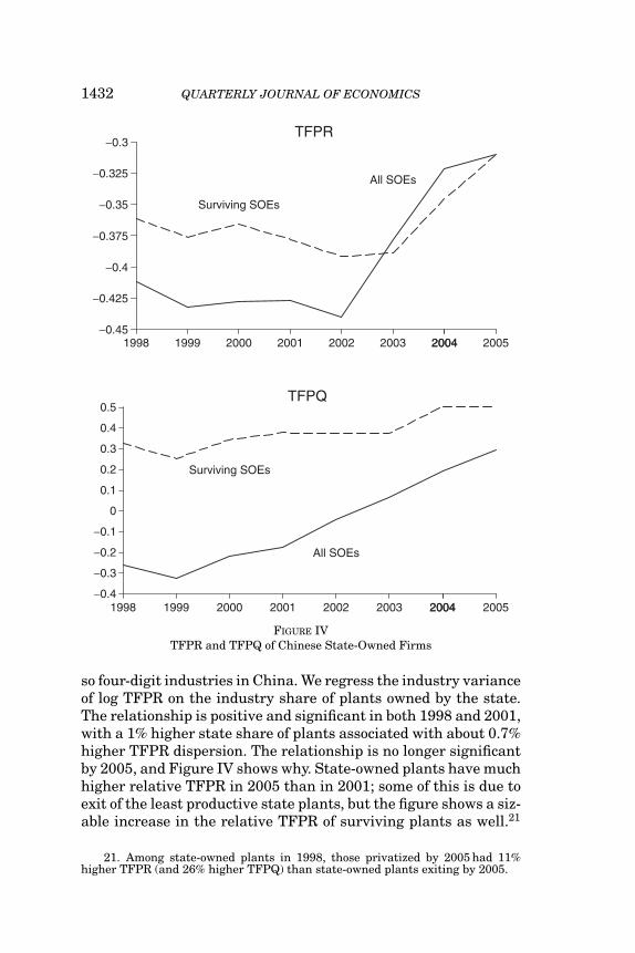
so four-digit industries in China. We regress the industry varianceof log TFPR on the industry share of plants owned by the state.The relationship is positive and significant in both 1998 and 2001,with a 1% higher state share of plants associated with about 0.7%higher TFPR dispersion. The relationship is no longer significantby 2005, and Figure IV shows why. State-owned plants have muchhigher relative TFPR in 2005 than in 2001; some of this is due toexit of the least productive state plants, but the figure shows a siz-able increase in the relative TFPR of surviving plants as well.21

21. Among state-owned plants in 1998, those privatized by 2005 had 11%higher TFPR (and 26% higher TFPQ) than state-owned plants exiting by 2005.


TABLE XIIIREGRESSION OF SECTOR TFPR DISPERSION ON DELICENSING AND SIZE RESTRICTIONS

IN INDIA

(1) (2) (3)

Delicensed 1991 −0.298 −0.298(0.117) (0.117)

Delicensed 1991 × post-1991 0.032 −0.056(0.036) (0.040)

Size restriction 0.368(0.173)

Delicensed 1991 × 0.415post 1991 × size restriction (0.120)

Notes. The dependent variable is the variance of log TFPR in sector s in year t. Entries are coefficientson the following independent variables: (1) delicensed 1991: indicator for whether industry was delicensedin 1991; (2) delicensed 1991 × post 1991: product of an indicator for an industry delicensed in 1991 andan indicator for observations after 1991; (3) size restriction: % of value-added of an industry subject toreservations for small firms and; (4) delicensed 1991 × post 1991 × size restriction: product of size restriction,indicator variable for observations after 1991, and a dummy variable for industries delicensed after 1991. Allregressions include indicator variables for year (1987 through 1994) and are weighted by the value-addedshare of the sector. Regressions (1) and (3) also include a dummy for industries delicensed in 1985. The omittedgroup consists of industries not delicensed in either 1985 or 1991. Standard errors are clustered by sector.Number of observations = 2,644.

When we equalize TFPR only within ownership categories, thegains are 8.2% lower in 1998 and 2.4% lower in 2005. Therefore,of the 15% reduction in potential gains from reallocation in Chinafrom 1998 to 2005, we calculate that 39% (5.8/15.0) comes fromthe shrinking TFPR gap between SOEs and other plants.

In India, misallocation within industries has often been at-tributed to licensing and size restrictions, among other govern-ment policies (see, e. g., Kochar et al. [2006]). These distortionsmay prevent efficient plants from achieving optimal scale andkeep inefficient plants from contracting or exiting. The Indiangovernment delicensed many industries in 1985 (about 40% ofindustries by value-added share) and in 1991 (about 42% of in-dustries by value-added share).22 India lifted its size restrictionsmuch more recently (1997–2005), which unfortunately we are un-able to analyze because our data end in 1994–1995. Across indus-tries during our sample, the mean share of industry value-addedsubject to size restrictions was 21% with a standard deviation of16%.23

In Table XIII we relate the dispersion of industry TFPR towhether the industry was delicensed in 1991 and to whether the

22. Based on three-digit data in Aghion et al. (2008).23. The list of industries subject to size restrictions is from Mohan (2002).


industry faced size restrictions. (We also include a dummy forindustries delicensed in 1985; the omitted group consists of in-dustries not delicensed in either 1985 or 1991.) The first columnshows that industries delicensed in 1991 exhibited less disper-sion of TFPR, but not in particular for 1991 onward. It is as iflicensed industries had lower TFPR dispersion despite their li-censing restrictions, and the delicensing did not affect this. Thereason may be that many of the delicensed industries were stillsubject to size restrictions. The second column of Table XIII indi-cates that the variance of log TFPR is greater within industriessubject to size restrictions. We interact delicensing with size re-strictions and years after 1991 in the third column, and find thatindustries delicensed in 1991 who face size restrictions do indeeddisplay more TFPR dispersion from 1991 onward. Delicensed in-dustries not facing size restrictions did exhibit lower TFPR from1991, but not significantly so.

India’s licensing restrictions might particularly restrict theability of plants to acquire inputs when their efficiency rises.If so, then we would expect plants with rising TFPQ to havehigher TFPR, but more so before delicensing than afterward.For Indian industries delicensed in 1991, Figure V plots aver-age log TFPR against percentiles of plant TFPQ growth, withboth variables relative to industry means. As predicted, the rela-tionship is positive but notably flatter after delicensing. WhereasTFPR differed by 1.2 log points across the 90th vs. 10th percentileTFPQ growth before delicensing, it differed by 0.6 log points afterdelicensing.

We find little evidence that TFPR dispersion is correlatedwith measures of geography, industry concentration, and (in In-dia) labor-market regulation. Average TFPR levels differ modestly(within 10%) across Chinese provinces and Indian states, so thatthe overwhelming majority of our TFPR differences are withinindustry regions. Within industry regions we tried without suc-cess to relate TFPR dispersion to industry concentration usinga Herfindahl index. For India we experimented with an index oflabor regulation for each industry, calculated as a weighted av-erage of the cumulative index of labor regulation in Besley andBurgess (2004) in each state, with weights equal to value-addedshares of each industry in each state. This index was not sig-nificantly related to the variance of log TFPR across industries,whether interacting with or controlling for delicensing and 1991onward.


−1.2

−1

−0.8

−0.6

−0.4

−0.2

0

0.2

0.4

0.6

0.8

10 25 50 75 90

Before delicensing

−1.2

−1

−0.8

−0.6

−0.4

−0.2

0

0.2

0.4

0.6

0.8

10 25 50 75 90

After delicensing

log T

FP

R

TFPQ growth (percentile)

FIGURE VTFPR and TFPQ Growth in Delicensed Sectors in India

VII. ALTERNATIVE EXPLANATIONS

We now entertain alternative explanations for TFPR disper-sion besides policy distortions and measurement error. Specif-ically, we briefly examine varying markups with plant size,adjustment costs, unobserved investments (such as R&D), andvarying capital elasticities within industries. All of these surelycontribute to TFPR dispersion in all three countries, but our ques-tion is whether they might explain the wider TFPR dispersion inChina and India than in the United States.


VII.A. Varying Markups with Plant Size

Our CES aggregation of plant value-added within industriesimplies that all goods have the same markup within industries(not to mention across industries). Yet markups might be higherfor bigger plants, and there may be greater size dispersion in ourChinese and Indian data than in the U.S. data. Markups are dis-tortions too, of course, but their dispersion may not wholly reflectpolicy differences between the countries. Melitz and Ottaviano(2008) analyze the case of linear demand, under which the elas-ticity of demand is falling (and the markup increasing) with size.Figure VI shows why we did not go this route. Whereas TFPR isstrongly increasing in percentiles of plant size (value added) in In-dia and mostly increasing in plant size in China, if anything TFPRdecreases with plant size in the United States. If linear demandapplied everywhere, then TFPR should increase with size in theUnited States, too. The fact that China and India differ not onlyquantitatively but qualitatively from the United States suggestsmore than just amplification of usual U.S. forces.

VII.B. Adjustment Costs

Young plants might have higher TFPR on average due toadjustment costs. If Chinese and Indian plants also differ in agemore than U.S. plants do, differences in adjustment costs by agecould contribute to wider TFPR dispersion in China and India.Figure VII plots average log TFPR (relative to industry means) bypercentile of plant age in each country. TFPR steadily increaseswith plant age in India, contrary to this story. In China, TFPRrises through the youngest decile, then is flat or mildly decreasingin the interdecile range before falling for the oldest decile. Onlythe United States exhibits the predicted pattern of steadily fallingTFPR with age.

More generally, growing plants might have higher TFPR thanshrinking plants because of adjustment costs. And input growthrates may vary more in China and India, because of their reforms,than in the United States with its more stable policy environ-ment. Figure VIII plots average TFPR by percentile of plant inputgrowth. TFPR is increasing in input growth in all three coun-tries, as predicted, but the United States exhibits more variationin TFPR associated with input growth than do China and India.Related, recall from Table X that input growth actually variesmore across U.S. plants than across plants in China or India. TheUnited States displays more churning, and so, if anything, should


−0.6

−0.4

−0.2

0

0.2

0.4

10 25 50 75 90

India

−0.6

−0.4

−0.2

0

0.2

0.4

10 25 50 75 90

China

−0.6

−0.4

−0.2

0

0.2

0.4

10 25 50 75 90

United States

log T

FP

R

Plant size (percentile)

FIGURE VITFPR and Size

have more TFPR variation because of convex adjustment costs ininput growth.24

Input growth may vary less in China and India because theirplants are hit with less volatile idiosyncratic shocks and/or be-cause they face higher adjustment costs. Cooper and Haltiwanger(2006) estimate idiosyncratic profitability shocks in a panel of U.S.

24. Another interpretation of Figure VIII is in terms of whether inputs arebeing reallocated to plants with higher TFPR. The answer is yes in all threecountries, but more so in the United States. This is consistent with more efficientresource allocation in the United States.


−0.4

−0.2

0

0.02

10 25 50 75 90

India

−0.4

−0.2

0

0.2

10 25 50 75 90

China

−0.4

−0.2

0

0.2

10 25 50 75 90

United States

log T

FP

R

Age (percentile)

FIGURE VIITFPR and Age

plants based on regressions of log profits (actually log revenueminus (roughly) 0.5 log capital) on its lagged value and year dum-mies. When we repeat their estimation for all three countries, weobtain similar estimates for the United States (serial correlation0.81, innovation standard deviation 0.56), China (0.79 and 0.59)and India (0.84 and 0.57). The overall standard deviation is 1%higher for China than the United States and 10% higher for Indiathan the United States. By comparison, in Table II the standarddeviations of TFPR are over 50% higher for China and India thanthe United States. Thus it would seem that plants in China and


−0.2

0

0.2

0.4

0.6

10 25 50 75 90

India

−0.2

0

0.2

0.4

0.6

10 25 50 75 90

China

−0.2

0

0.2

0.4

0.6

10 25 50 75 90

United States

log T

FP

R

Input growth (percentile)

FIGURE VIIITFPR and Input Growth

India face greater barriers to reallocation as opposed to biggershocks with the same costs of reallocation.

Figure VII related average TFPR to plant age. A related hy-pothesis is that young (or small) plants display greater disper-sion of TFPR. If plants in China or India are younger or smallerthan U.S. plants, therefore, then one might expect them to dis-play more variable TFPR. Table XIV provides the age of the 25th,50th, and 75th percentile plants in each country. Chinese plants


TABLE XIVDISTRIBUTION OF PLANT AGE (PERCENTILES)

25th 50th 75th

China 2 5 22India 6 12 22United States 5 10 25

Notes. Entries are the 25th, 50th, and 75th percentile distribution of plant age in a sector, where eachsector is weighted by the value-added share of the sector.

(median age five years) are younger than U.S. plants (median ageten years), but Indian plants are older (median age twelve years).Figure IX plots the size (employment) distribution of plants inall three countries. Indian plants (median size 33 employees) aresmaller than U.S. plants (median size 47 employees), but Chi-nese plants (median size 160 employees) are much larger thanU.S. plants. When we split plants into quartiles of size and age(respectively) and equalize TFPR only within quartiles, the gainsare about 5% lower for both China and India. Thus variation inTFPR by size and age explains only a modest amount of the overalldispersion in TFPR (see Table III).

VII.C. Unobserved Investments

Low TFPR might reflect learning by doing or other unob-served investments (R&D, building a customer base) rather thandistortions. If so, then we expect low-TFPR plants to exhibit highsubsequent TFPQ growth. Figure X displays precisely this pat-tern in the United States, but the opposite pattern in China andIndia. Thus it is far from obvious that unobserved plant invest-ments vary more in China and India than in the United States. IfTFPQ growth does proxy for unobserved investments, then FigureX suggests that such investments may mitigate TFPR differencesin China and India.

Perhaps related, TFPR differences are more transitory in theUnited States than in China and India (see the “IV” results dis-cussed near the end of Section V). U.S. TFPR differences maylargely reflect temporary differences in investments and adjust-ment costs, whereas TFPR differences in China and India mayreflect more persistent, perhaps policy-related gaps that are notas reliably closed with subsequent input reallocation and TFPQgrowth.


0

0.05

0.1

0.15

0.2

0.25

1 4 16 64 256 1,024 4,096 16,384

India

0

0.05

0.1

0.15

0.2

0.25

1 4 16 64 256 1,024 4,096 16,384

China

0

0.05

0.1

0.15

0.2

0.25

1 4 16 64 256 1,024 4,096 16,384

United States

FIGURE IXDistribution of Number of Workers

VII.D. Varying Capital Shares within Industries

Our baseline estimates in Table VI assumed the same capitalelasticity for all plants within a four-digit industry. We inferredrelative distortions from variation in capital-labor ratios withinindustries. At the other extreme, one could attribute all variationin these ratios within industries to plant-specific capital shares.Doing so and recalculating the TFP gains, we find the majority ofthe gains in China and India relative to the United States stemfrom output distortions. With plant-specific capital shares, TFP


−0.4

−0.2

0

0.2

0.4

0.6

10 25 50 75 90

India

−0.4

−0.2

0

0.2

0.4

0.6

10 25 50 75 90

China

−0.4

−0.2

0

0.2

0.4

0.6

10 25 50 75 90

United States

log T

FP

R

TFPQ growth (percentile)

FIGURE XTFPR and TFPQ Growth

gains are still 23%–45% (vs. 30%–50% baseline) for China and32%–39% (vs. 40%–60% baseline) for India.

VIII. CONCLUSION

A long stream of papers has stressed that misallocation ofinputs across firms can reduce aggregate TFP in a country. Weused microdata on manufacturing plants to investigate the pos-sible role of such misallocation in China (1998–2005) and India(1987–1994) compared with the United States (1977, 1987, 1997).


Viewing the data through the prism of a standard monopolisticcompetition model, we estimated differences in marginal prod-ucts of labor and capital across plants within narrowly definedindustries. We found much bigger gaps in China and India thanin the United States. We then entertained a counterfactual moveby China and India to the U.S. dispersion of marginal products.We found that this would boost TFP by 30%–50% in China andby 40%–60% in India. Room for reallocation gains shrank about2% per year from 1998–2005 in China, as if reforms there reapedsome of the gains. In India, despite reforms in the early 1990s, wereport evidence of rising misallocation from 1991 to 1994.

Our results require many caveats. There could well be greatermeasurement error in the Chinese and Indian data than in theU.S. data. The static monopolistic competition model we deploycould be a poor approximation of all three countries. Although weprovided reassuring evidence on these concerns, our investigationwas very much a first pass. In addition to investigating these is-sues more fully, future work could try to relate differences in plantproductivity to observable policy distortions much more than wehave. Finally, we neglected the potential impact of distortions onplant entry and exit, an important topic for future research.

APPENDIX I: LUCAS SPAN-OF-CONTROL VERSION

In the main text we modeled manufacturing plants as mo-nopolistic competitors, and related the elasticity of substitutionbetween varieties to a large empirical literature. However, manymodelers, such as Restuccia and Rogerson (2008), follow Lucas(1978) in positing diminishing returns in production rather thanutility. Here we show how the two formulations are isomorphic foraggregate TFP for a given number of plants and aggregate laborinput.

Suppose labor is the sole input and there is a single sector.The equations for aggregate output, firm output, and firm profitsfor each variety are

Y =M∑

i=1

Yi,

Yi = Ai Lγ

i ,

πi = (1 − τi)PYi − wLi.


Returns to scale equal γ , and P is the price of homogeneous output.TFP (=Y/L here) is

TFP =⎡⎣ M∑

i=1

(TFPQi

(TFPRTFPRi

)) 11−γ

⎤⎦

1−γ /L1−γ .

Here TFPQi = Ai and TFPRi = 1/(1 − τ i). This is the same asour expression in the main text, except for two differences. First,1/(1 − γ ) takes the place of (σ − 1). Diminishing returns in pro-duction (γ < 1) play the same role as diminishing returns in utility(σ < ∞). Second, aggregate TFP is now decreasing in aggregatelabor input. If the number of plants is proportional to labor input,then such aggregate decreasing returns disappear. Of course, avariety benefit would then exist in the CES formulation. In termsof our calibration, our conservative choice of σ = 3 corresponds toγ = 0.5. This is quite low, even compared to studies such as Atke-son and Kehoe (2005), who chose γ ≥ 0.8 based on diminishingreturns in both production and utility.

APPENDIX II: GENERALIZING TFPQ FOR QUALITY AND VARIETY

Here we sketch how our measure of TFPQ should capturenot only process efficiency but also firm differences in qualityand variety (equivalently, idiosyncratic demand). For simplicity,suppose labor is the sole input and there is a single sector. Theequations for aggregate output, firm output, and firm profits foreach variety are

Y =[

M∑i=1

Ni (Qi Yi/Ni)σ−1

σ

] σσ−1

,

Yi = Ai Li,

πi = (1 − τi)PiYi − wLi.

Here Ni is the number of symmetric varieties the firm produces, Qi

is the symmetric quality of each of its varieties, Ai is its processefficiency, Yi/Ni is the symmetric quantity it produces of eachvariety, and Pi is the symmetric price of each variety. For thiseconomy, our method of measuring TFPQ yields

TFPQi = (PiYi)σ

σ−1 /Li

Y1

σ−1 Pσ

σ−1

= Ai Qi N1

σ−1i .


Measured TFPQ is a composite of process efficiency and idiosyn-cratic demand terms coming from quality and variety. AggregateTFP (=Y/L here) is identical to the case in which firms vary onlyin process efficiency, only with the above measure of TFPQ:

TFP = TFPQ =⎧⎨⎩

M∑i=1

[TFPQi

(TFPRTFPRi

)]σ−1⎫⎬⎭

1σ−1

.

TFPR is as in the main text, only here it reduces to the singledistortion, TFPRi = 1/(1 − τ i). Note that aggregate TFP (effectiveoutput per worker) is also synonymous with welfare.

APPENDIX III: LABOR AND CAPITAL DISTORTIONS

In the main text we estimated distortions to output (τY si)and to capital relative to labor (τKsi), respectively. An observa-tionally equivalent characterization is in terms of distortions tothe absolute levels of capital and labor. Denote level distortionsas τ ∗

Lsi and τ ∗Ksi, and profits as πsi = PsiYsi − (1 + τ ∗

Lsi)wLsi − (1 +τ ∗

Ksi)RKsi. The firm’s first-order conditions are identical to thosewith {τY si, τKsi} assuming 1 − τY si = 1/(1 + τ ∗

Lsi) and 1 + τKsi =(1 + τ ∗

Ksi)/(1 + τ ∗Lsi). Sectoral TFP is identical under these condi-

tions as well.We denote deviations of plant variables from industry-

weighted means as

�Asi = lnAsi

As,�τ ∗

Lsi = ln1 + τ ∗

Lsi

1 + τ ∗Ls

,�τ ∗Ksi = ln

1 + τ ∗Ksi

1 + τ ∗Ks

,

�Lsi = lnwLsi∑Ms

i=1 wLsi/Ms

.

For the latest years in China and India, the correlation ma-trices of these variables are shown in Table A.1. Not surprisingly,plants with high TFPQ tend to have high labor input. More in-teresting, plants with high TFPQ typically face higher “taxes” onboth capital and labor. The distortions discourage labor input, butnot strongly, because, again, the distortions tend to be high whenTFPQ would dictate high labor input. Labor and capital wedgesare positively correlated across plants, but only modestly so.

Here we can entertain the thought experiment of eliminatingvariation in the capital or labor distortion individually. For thelatest year in China, the TFP gains from eliminating the capital


TABLE A.1

China 2005 India 1994

�Asi �τ ∗Lsi �τ ∗

Ksi �Asi �τ ∗Lsi �τ ∗

Ksi

�Lsi 0.518 −0.202 −0.074 0.690 0.010 −0.038�τ ∗

Lsi 0.532 1 0.201 0.538 1 0.004�τ ∗

Ksi 0.592 0.201 1 0.398 0.004 1

(labor) distortion alone are 60% (24%) compared to 87% from elim-inating both distortions. In India, the gains from eliminating thecapital (labor) distortion alone are 78% (33%) compared to 128%from eliminating both distortions.

UNIVERSITY OF CHICAGO BOOTH SCHOOL OF BUSINESS AND NBERSTANFORD UNIVERSITY, SIEPR, SCID, AND NBER

REFERENCES

Aghion, Philippe, Robin Burgess, Stephen Redding, and Fabrizio Zilibotti, “TheUnequal Effects of Liberalization: Evidence from Dismantling the LicenseRaj in India,” American Economic Review, 98 (2008), 1397–1412.

Alfaro, Laura, Andrew Charlton, and Fabio Kanczuk, “Plant-Size Distributionand Cross-Country Income Differences,” NBER Working Paper No. w14060,2008.

Allen, Franklin, Rajesh Chakrabarti, Sankar De, Jun “QJ” Qian, and Meijun Qian,Financing Firms in India, manuscript, University of Pennsylvania, 2007.

Atkeson, Andrew G., and Patrick J. Kehoe, “Modeling and Measuring Organiza-tional Capital,” Journal of Political Economy, 113 (2005), 1026–1053.

Banerjee, Abhijit, and Esther Duflo, “Growth Theory through the Lens of Develop-ment Economics,” in Handbook of Economic Growth, Vol. 1 A, P. Aghion andS. Durlauf, eds. (Amsterdam: Elsevier, 2005, Chap. 7).

Barro, Robert, J., and Jong-Wha Lee, “International Data on Educational Attain-ment: Updates and Implications,” NBER Working Paper No. w7911, 2000.

Bartelsman, Eric, John Haltiwanger, and Stefano Scarpetta, Cross-Country Differ-ences in Productivity: The Role of Allocative Efficiency, manuscript,Universityof Maryland, 2008.

Bergoeing, Raphael, Patrick J. Kehoe, Timothy J. Kehoe, and Raimundo Soto,Review of Economic Dynamics, 5 (2002), 166–205.

Besley, Timothy, and Robin Burgess, “Can Labor Regulation Hinder Economic Per-formance? Evidence from India,” Quarterly Journal of Economics, 119 (2004),91–134.

Bosworth, Barry, and Susan M. Collins, “Accounting for Growth: Comparing Chinaand India,” NBER Working Paper No. w12943, 2007.

Broda, Christian, and David E. Weinstein, “Globalization and the Gains fromVariety,” Quarterly Journal of Economics, 121 (2006), 541–585.

Buera, Francisco, and Yongseok Shin, Financial Frictions and the Persistence ofHistory: A Quantitative Exploration, manuscript, University of California,Los Angeles, 2008.

Caselli, Francesco, “Accounting for Income Differences across Countries,” in Hand-book of Economic Growth, Vol. 1 A, P. Aghion and S. Durlauf, eds. (Amsterdam:Elsevier, 2005, Chap. 9).


Caselli, Francesco, and Nicola Gennaioli, “Dynastic Management,” NBER WorkingPaper No. w9442, 2003.

Chari, V. V., Patrick J. Kehoe, and Ellen C. McGrattan, “Business Cycle Account-ing,” Econometrica, 75 (2007), 781–836.

Cooper, Russell W., and John C. Haltiwanger, “On the Nature of Capital Adjust-ment Costs,” Review of Economic Studies, 73 (2006), 611–633.

Dobson, Wendy, and Anil K. Kashyap, “The Contradiction in China’s Gradual-ist Banking Reforms,” Brooking Papers on Economic Activity, 2 (2006), 103–148.

Dollar, David, and Shang-jin Wei, “Das (Wasted) Kapital: Firm Ownership andInvestment Efficiency in China,” NBER Working Paper No. w13103, 2007.

The Economist, “Survey: Business in India,” June 3, 2006a. Available online athttp://www.economist.com/surveys/displayStory.cfm?story id=6969740.

——, “Survey: China,” May 23, 2006b. Available online at http://www.economist.com/surveys/displayStory.cfm?story id=5623226.

Farrell, Diana, and Susan Lund, “China’s and India’s Financial Systems: A Barrierto Growth,” McKinsey Quarterly, November (2006), 1–12.

Foster, Lucia, John Haltiwanger, and Chad Syverson, “Reallocation, FirmTurnover, and Efficiency: Selection on Productivity or Profitability?” Amer-ican Economic Review, 98 (2008), 394–425.

Galindo, Arturo, Fabio Schiantarelli, and Andrew Weiss, “Does Financial Liberal-ization Improve the Allocation of Investment? Micro-Evidence from Develop-ing Countries,” Journal of Development Economics, 83 (2007), 562–587.

Guner, Nezih, Gustavo Ventura, and Yi Xu, “Macroeconomic Implications of Size-Dependent Policies,” Review of Economic Dynamics, 11 (2008), 721–744.

Hall, Robert E., and Charles I. Jones, “Why Do Some Countries Produce So MuchMore Output per Worker Than Others?” Quarterly Journal of Economics, 114(1999), 83–116.

Hallward-Driemeier, Mary, Giuseppe Iarossi, and Kenneth L. Sokoloff, “Exportsand Manufacturing Productivity in East Asia: A Comparative Analysis withFirm-Level Data,” NBER Working Paper No. w8894, 2002.

Hendel, Igal, and Aviv Nevo, “Measuring the Implications of Consumer InventoryBehavior,” Econometrica, 74 (2006), 1637–1673.

Hopenhayn, Hugo, and Richard Rogerson, “Job Turnover and Policy Evaluation:A General Equilibrium Analysis,” Journal of Political Economy, 101 (1993),915–938.

Howitt, Peter, “Endogenous Growth and Cross-Country Income Differences,” Amer-ican Economic Review, 90 (2000), 829–846.

Klenow, Peter J., and Andres Rodrıguez-Clare, “The Neoclassical Revival inGrowth Economics: Has It Gone Too Far?” in NBER Macroeconomics Annual,B. Bernanke and J. Rotemberg, eds. (Cambridge, MA: MIT Press, 1997).

——, “Externalities and Economic Growth,” in Handbook of Economic Growth, Vol.1 A, P. Aghion and S. Durlauf, eds. (Amsterdam: Elsevier, 2005, Chap. 11).

Kochar, Kalpana, Utsav Kumar, Raghuram Rajan, Arvind Subramanian, and Ioan-nis Tokatlidis, “India’s Pattern of Development: What Happened, What Fol-lows,” NBER Working Paper No. w12023, 2006.

Lagos, Ricardo, “A Model of TFP,” Review of Economic Studies, 73 (2006), 983–1007.Lewis, William W., The Power of Productivity: Wealth, Poverty, and the Threat to

Global Stability (Chicago: University of Chicago Press, 2004).Lucas, Robert E., Jr., “On the Size Distribution of Business Firms,” Bell Journal

of Economics, 9 (1978), 508–523.McKinsey Global Institute, Productivity: The Key to an Accelerated Development

Path for Brazil (Washington, DC: McKinsey Global Institute, 1998).Melitz, Marc J., “The Impact of Trade on Intra-Industry Reallocations and Aggre-

gate Industry Productivity,” Econometrica, 71 (2003), 1695–1725.Melitz, Marc J., and Gianmarco I. P. Ottaviano, “Market Size, Trade, and Produc-

tivity,” Review of Economic Studies, 75 (2008), 295–316.Mohan, Rakesh, “Small Scale Industry in India: A Critical Evaluation,” in Eco-

nomic Policy Reforms and the Indian Economy, Anne Krueger, ed. (Chicago:University of Chicago Press, 2002).

Parente, Stephen L., and Edward C. Prescott, Barriers to Riches (Cambridge, MA:MIT Press, 2000).


Restuccia, Diego, and Richard Rogerson, “Policy Distortions and Aggregate Pro-ductivity with Heterogeneous Plants,” Review of Economic Dynamics, 11(2008), 707–720.

Young, Alwyn, “The Razor’s Edge: Distortions and Incremental Reform in thePeople’s Republic of China,” Quarterly Journal of Economics, 115 (2000), 1091–1135.

——, “Gold into Base Metals: Productivity Growth in the People’s Republic ofChina during the Reform Period,” Journal of Political Economy, 111 (2003),1220–1261.

the quarterly journal of economicsklenow.com/mmtfp.pdf · the quarterly journal of economics vol....

Documents