HAL Id: hal-01824491https://hal.archives-ouvertes.fr/hal-01824491

Submitted on 27 Jun 2018

HAL is a multi-disciplinary open accessarchive for the deposit and dissemination of sci-entific research documents, whether they are pub-lished or not. The documents may come fromteaching and research institutions in France orabroad, or from public or private research centers.

L’archive ouverte pluridisciplinaire HAL, estdestinée au dépôt et à la diffusion de documentsscientifiques de niveau recherche, publiés ou non,émanant des établissements d’enseignement et derecherche français ou étrangers, des laboratoirespublics ou privés.

The proper use of mass diffusion equation in dryingmodelling: from simple configurations to non-fickian

behavioursPatrick Perre

To cite this version:Patrick Perre. The proper use of mass diffusion equation in drying modelling: from simple configu-rations to non-fickian behaviours. 19th International Drying Symposium IDS’2014, Aug 2014, Lyon,France. �hal-01824491�

19th International Drying Symposium (IDS 2014) Lyon, France, August 24-27, 2014

THE PROPER USE OF MASS DIFFUSION EQUATION IN DRYING MODELLING: FROM SIMPLE CONFIGURATIONS TO NON-FICKIAN BEHAVIOURS

Patrick Perré

Ecole Centrale Paris, LGPM Laboratoire de Génie des Procédés et Matériaux

Grande Voie des Vignes, 92290 Châtenay-Malabry, France

E-mail: patrick.perre@ecp.fr

Abstract: This keynote paper intends to clearly define the possibilities and limitations offered by a simple diffusion approach of drying. Actually, many works use a simple diffusion equation to model mass transfer during drying, probably because a simple analytical solution of this equation does exist in the case of simple boundary conditions. However, one has to be aware of the limitations of this approach. Using a comprehensive formulation and a relevant computational solution, the most frequent assumptions of the diffusion approach were rigorously tested. It is concluded that analytical solutions must be discarded for several reasons: - Dirichlet boundary conditions are not realistic, - In the drying process, the coupling between heat and mass transfer is mandatory, - Non-linearity (variation of diffusivity with moisture content) cannot be avoided for

mass transfer. The second part of the paper is devoted to the solution of configurations that exhibit a non-Fickian behavior. The first case study concerns the long-term behavior of wood during transient diffusion. Explained by the mobility of macromolecules, this behavior can be formulated through relevant boundary conditions. The second example shows how a diffusion equation solved in a dual-scale porous medium is able to produce a non-Fickian behavior at the macroscopic scale.

Keywords: boundary conditions, external transfer, heat and mass transfer, multiscale.

INTRODUCTION A historical perspective on the formulation of coupled heat and mass transfer in porous media is a good introduction to the topic of this paper. It is worthwhile to remember that the widespread formulation of transfers in the form of differential equations was launched about 200 years ago. This approach started with the heat transfer by conduction, formulated and solved by Fourier in 1822[1]. Mass transfer, in continuum media and in porous media, was formulated with similar expressions at the end of the 19th century (Fick, 1855, Darcy 1856)[2,3]. Following these outstanding advances in the formulation of continuous media, a scientific approach of drying was initiated at the beginning of the 20th century. Lewis(1921)[4] describes drying as the combination of two mechanisms: humidity evaporation at the exchange surface and moisture diffusion within the solid. In 1929, in a paper entitled "The drying of solids"[5] Sherwood describes the

drying as a combination of internal and external resistance to transfer. At this time, the nature of migration within the porous medium was the object of active discussion. A diffusion equation gave nice results for some materials (clay and wood in the hygroscopic range for example), but failed in other cases. The importance of capillary forces was definitely proved in the case of sand by Ceaglske and Hougen (1937)[6]. In this work, the moisture content profiles during drying were analyzed as quasi-equilibrated moisture content profiles due to gravity. Nevertheless, none of these expressions, diffusion or capillary action, could be applied to all configurations. The need for a more comprehensive formulation became obvious.

In the fifties, comprehensive sets of equations were proposed from the analysis of careful experiments by Krischer's school in Germany[7]. Some years later, from their works on transfer in soils, Philips and de Vries[8] proposed a comprehensive set of coupled transfer in porous media. In USSR, Luikov[9]

produced an important work, especially in the mathematical formulation of coupled heat and mass transfer(1). In the sets of equations resulting from these three schools, most coupled phenomena involved in heat and mass transfer were considered: moisture migration due to a gradient of moisture content, thermo-migration, capillary forces, latent heat of vaporization in the energy balance…

Finally, the "modern" way to formulate heat and mass transfer in porous media was open in 1977 by Whitaker[10], who derived a justification of the macroscopic formulation from the microscopic level using the volume averaging technique published by Slattery some years earlier[11].

COMPREHENSIVE FORMULATION OF HEAT AND MASS TRANSFER IN POROUS MEDIA

Coupled and simultaneous heat, mass and momentum transfer in porous media is a complex problem, which requires the development of transport equations derived from the standard conservation laws inside each phase and fluxes at the phase interfaces. The challenge, however, is to overcome the problems associated with structural dependencies and the complex geometries evident in the internal pore network within the medium. Typically, transport phenomena are represented according to macroscopic equations valid at the relevant level of description.

Fig. 1. Concept of Representative Elementary Volume (REV) [17].

This assumes the variables to be defined at the level of many pores and the porous material to be represented as a fictitious continuum[12]. In this framework, it is possible to rigorously derive the macroscopic equations from microscopic balance equations by means of volume averaging[10,11,13-15].

1Unfortunately, Luikov's formulation involves the so-called phase conversion factor of liquid into vapour, which is not an intrinsic parameter and drove several scientists on a misleading track.

Fig. 2. The averaging method assumes the existence of a representative elementary volume, large enough for the pore effect to be smoothed and small enough

for macroscopic variations and non-equilibrium effects to be avoided. The examples here are for

density (point 1 is in the solid phase and point 2 in a pore) [17].

The underlying idea of volume averaging[11,16] is to average the dependent variable (for example liquid or the gas phase water vapor density) over some representative localized volume, as depicted in figure 1. The averaging volume V (REV) comprises the individual phase volumes each of which can vary with space, as well as time for the liquid and gas phases. Averages are then defined in terms of these volumes and are said to be associated with the centroid of the averaging volume V, which assumes the existence of a representative volume that is large enough for the averaged quantities to be defined and small enough to avoid variations due to macroscopic gradients and non-equilibrium configurations at the microscopic level (Fig. 2). The development of the volume averaged transport equations requires the introduction of what are called superficial and intrinsic averages. For example, the superficial average of the density of the liquid phase is given by

ρw = 1V

ρwVw∫ dV (1)

and its intrinsic average by

ρww = 1Vw

ρwVw∫ dV (2)

Where wV is the volume of the liquid phase contained inV . One also notes the relationship ρw = εwρw

w in which εw =Vw /V is the volume

fraction of the liquid phase. The latter average is claimed to be the best representation in the sense that if ρw were a constant given by ρw

0 , then the intrinsic

average gives ρww = ρw

0 , whereas the superficial

average gives ρw = εwρw0 .

The derivation of macroscopic equations starts with classical laws of conservation (mass, energy, momentum) for each phase. The average of these equations over the REV needs rules to obtain spatial and temporal derivatives. This gives rise to equations with fluctuations terms that requires closure equations to be solved[10,14]. The whole procedure assumes the separation of scales (Fig. 2). The comprehensive set of macroscopic equations resulting from this volume averaging procedure and adapted to the case of hygroscopic products reads as follows[14,17,18].

Moisture conservation

∂ εwρw + εgρvg + ρb( )

∂t+∇· ρwvw + ρv

gvg + ρbvb( )= ∇· ρgDeff ·∇ωv( )

(3)

Energy conservation

∂∂t

εwρwhw + εg (ρvghv + ρa

gha )

+ρbhb + εsρshs − εg pg

⎛

⎝⎜⎜

⎞

⎠⎟⎟

+∇· ρwhwvw + (ρvghv + ρa

gha )vg + hbρbvb( )+ vw·∇pw + vg·∇pg

= ∇· ρgDeff (hv∇ωv + ha∇ωa ) + λeff∇T( )

(4)

Air conservation

∂ εgρag( )

∂t+∇· ρa

gvg( ) = ∇· ρgDeff∇ωa( ) (5)

In the following equation, the barycentric mass velocities comes from the generalized Darcy's law

vg = −Kkgµg

(∇pg − ρg∇ψ g )

vw = −Kkwµw

(∇pw − ρw∇ψ g )

with pw = pg − pc (X ,T )

(6)

In equation (6), ψ g stands for the potential energy

associated to gravity. In the case of almost isothermal media, such as in convective drying, all possible driving forces for the

bound water migration are equivalent. This is why the simplest one, i.e. the gradient of bound water density (first expression in equation 7), has been widely used by the author. However, in the presence of a thermal gradient, the choice of the relevant driving force is a serious concern, still open in spite of numerous works devoted to this question. Recent experimental results[19, 20] tends to prove that the gradient of water vapor density in the gaseous phase (second expression in the following equation) is a relevant choice

ρbvb = −Db,X∇ρb = −Db,ρv∇ρv

g (7)

Boundary conditions For the external drying surfaces of the sample, the boundary conditions are assumed to be of the following form:

Jv x=0+·n = hm cMv ln1− xv,∞1− xv x=0

⎛

⎝⎜⎜

⎞

⎠⎟⎟

Jq x=0+·n = h (T x=0−T∞ )

Pg x=0+= Patm

(8)

where Jv and Jq represent the fluxes of water vapor and heat at the boundary respectively, x denotes the position from the boundary along the external unit normal. Remark: The previous set of equations assumes that the porous medium is locally at equilibrium. This implies that: - the temperature is the same for all phases Tss = Tw

w = Tgg

- the partial pressure of water vapor inside the gaseous phase is related to the moisture content Xvia the sorption isotherm pv = pvs(T )×a(T ,X ) , where the function a is the sorption isotherm of the product, also called water activity, namely in food science. Further simplifications or assumptions allow this set of equations to take a more convenient form: - the variations of partial densities inside the REV are negligible, so the intrinsic average is equal to the local value ρv

g = ρv and ρag = ρa ,

- the solid density is assumed to be constantρs = constant , - the moisture content X is used to consider the total amount of water present in the porous mediumρsX = εwρw + εgρv

g + ρb ,

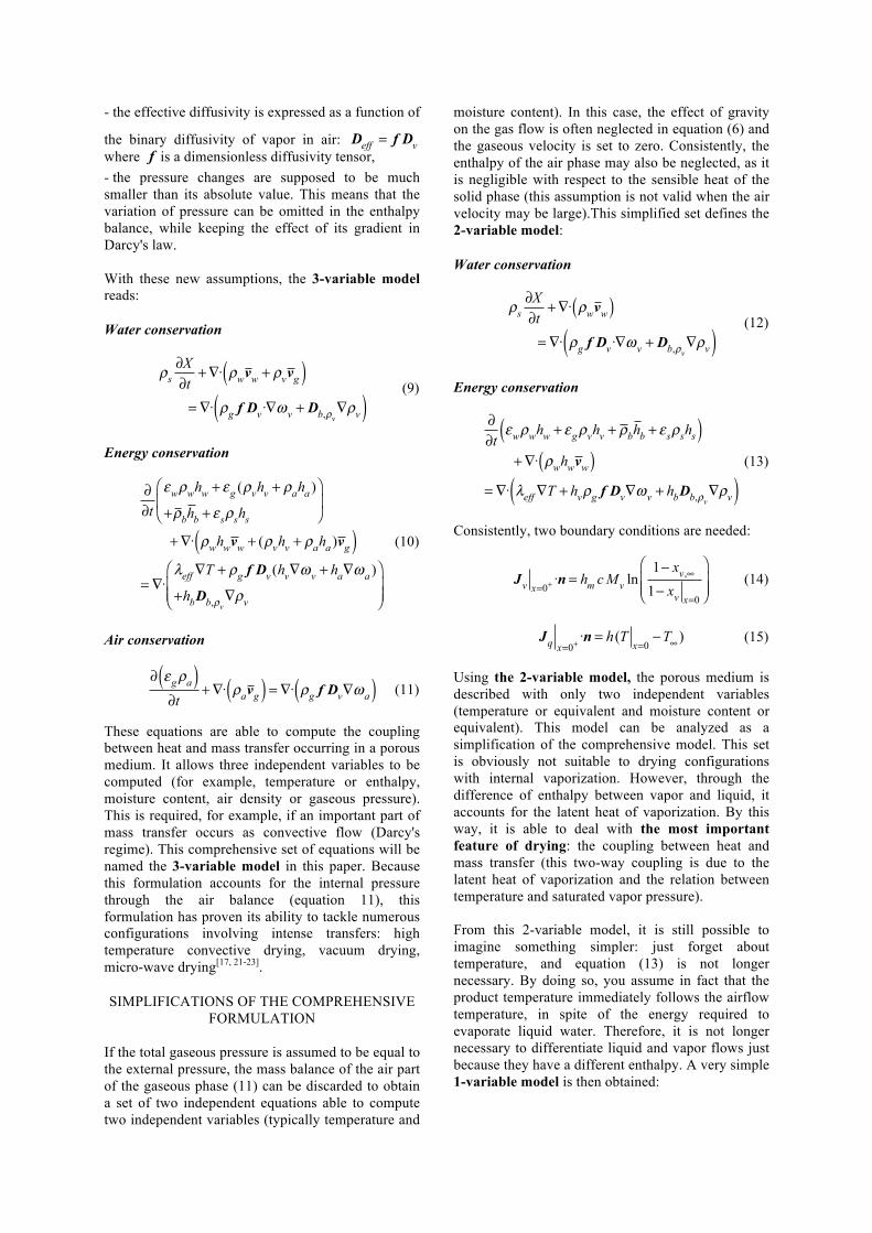
- the effective diffusivity is expressed as a function of

the binary diffusivity of vapor in air: Deff = f Dvwhere f is a dimensionless diffusivity tensor, - the pressure changes are supposed to be much smaller than its absolute value. This means that the variation of pressure can be omitted in the enthalpy balance, while keeping the effect of its gradient in Darcy's law. With these new assumptions, the 3-variable model reads:

Water conservation

ρs

∂X∂t

+∇· ρwvw + ρvvg( )= ∇· ρg f Dv·∇ωv + Db,ρv∇ρv( )

(9)

Energy conservation

∂∂t

εwρwhw + εg (ρvhv + ρaha )

+ρbhb + εsρshs

⎛

⎝⎜

⎞

⎠⎟

+∇· ρwhwvw + (ρvhv + ρaha )vg( )= ∇·

λeff∇T + ρg f Dv (hv∇ωv + ha∇ωa )

+hbDb,ρv∇ρv

⎛

⎝⎜⎜

⎞

⎠⎟⎟

(10)

Air conservation

∂ εgρa( )∂t

+∇· ρavg( ) = ∇· ρg f Dv∇ωa( ) (11)

These equations are able to compute the coupling between heat and mass transfer occurring in a porous medium. It allows three independent variables to be computed (for example, temperature or enthalpy, moisture content, air density or gaseous pressure). This is required, for example, if an important part of mass transfer occurs as convective flow (Darcy's regime). This comprehensive set of equations will be named the 3-variable model in this paper. Because this formulation accounts for the internal pressure through the air balance (equation 11), this formulation has proven its ability to tackle numerous configurations involving intense transfers: high temperature convective drying, vacuum drying, micro-wave drying[17, 21-23].

SIMPLIFICATIONS OF THE COMPREHENSIVE FORMULATION

If the total gaseous pressure is assumed to be equal to the external pressure, the mass balance of the air part of the gaseous phase (11) can be discarded to obtain a set of two independent equations able to compute two independent variables (typically temperature and

moisture content). In this case, the effect of gravity on the gas flow is often neglected in equation (6) and the gaseous velocity is set to zero. Consistently, the enthalpy of the air phase may also be neglected, as it is negligible with respect to the sensible heat of the solid phase (this assumption is not valid when the air velocity may be large).This simplified set defines the 2-variable model:

Water conservation

ρs

∂X∂t

+∇· ρwvw( )= ∇· ρg f Dv·∇ωv + Db,ρv∇ρv( )

(12)

Energy conservation

∂∂t

εwρwhw + εgρvhv + ρbhb + εsρshs( )+∇· ρwhwvw( )

= ∇· λeff∇T + hvρg f Dv∇ωv + hbDb,ρv∇ρv( ) (13)

Consistently, two boundary conditions are needed:

Jv x=0+·n = hm cMv ln1− xv,∞1− xv x=0

⎛

⎝⎜⎜

⎞

⎠⎟⎟

(14)

Jq x=0+·n = h (T x=0−T∞ ) (15)

Using the 2-variable model, the porous medium is described with only two independent variables (temperature or equivalent and moisture content or equivalent). This model can be analyzed as a simplification of the comprehensive model. This set is obviously not suitable to drying configurations with internal vaporization. However, through the difference of enthalpy between vapor and liquid, it accounts for the latent heat of vaporization. By this way, it is able to deal with the most important feature of drying: the coupling between heat and mass transfer (this two-way coupling is due to the latent heat of vaporization and the relation between temperature and saturated vapor pressure). From this 2-variable model, it is still possible to imagine something simpler: just forget about temperature, and equation (13) is not longer necessary. By doing so, you assume in fact that the product temperature immediately follows the airflow temperature, in spite of the energy required to evaporate liquid water. Therefore, it is not longer necessary to differentiate liquid and vapor flows just because they have a different enthalpy. A very simple 1-variable model is then obtained:

Water Conservation

∂X∂ t

= ∇⋅ Dp(X )∇X( ) (16)

Equation (16) is often known as “second Fick’s law”, which combines the Fick’s law of mass transfer due to a concentration gradient with the mass conservation equation. In this equation, as no temperature gradient now exists inside the product, one single driving force subsists: the gradient of moisture content. The pseudo-diffusivity tensor Dp can be expressed using equations (6), (7) and (9) provided it is assumed that the gravity field has negligible effect on moisture migration:

Dp (X ) = −ρwKkwµw

∂pc (X ,T )∂X

+ f Dv (T ) + Db,ρv (X ,T )( ) pvs(T )MvRT

∂a(X ,T )∂X

(17)

In equation (17), the temperature remains involved as a parameter able to account for thermo-activation of - liquid flow : effect of temperature on the surface

tension of water, - vapor and bound water diffusion : effect of

temperature on the binary diffusivity, bound water diffusion and sorption isotherm, and, above all, the dependence of saturated water vapor with temperature.

In addition, it becomes obvious from this expression that equation (16) is a non-linear equation: the pseudo-diffusivity coefficient depends on moisture content. In most products, this dependence is known to be strong: the overall moisture diffusivity increases dramatically with moisture content.

Boundary conditions Equation (14) is the proper physical formulation for vapor flow in the convective boundary layer. However, when the simple 1-variable model is used, the following boundary conditions is often used

Jv x=0+ ⋅ n̂ = hX (Xsurf − Xeq ) (18)

where Xh is a pseudo mass transfer coefficient, that may be calculated from equation (8), surfX is the

moisture content at the exchange surface and eqX the equilibrium moisture content as obtained from temperature and relative humidity of the surrounding air. Note that equation (18) is not strictly equivalent to equation (14). Indeed, while the surface of the porous medium remains in the domain of free liquid (first drying period), the vapor pressure at surface is constant, equal to the saturated vapor pressure. The driving force for the external vapor flux in equation

(14) is therefore constant during the first drying period whereas it decreases in equation (18) as drying progresses. Equations (16-18) - or (14, 16, 17) - define the drying of a product with one variable, the moisture content field. This simple set summarizes what is called the diffusion approach of drying. If we remember that the objective of drying is to remove the moisture from the product, the concept of a 1-variable model sounds relevant: it accounts for the moisture migration within the medium and the moisture flux at the boundary. In addition, a simple analytical solution exists for this equation in 1-D. Both arguments probably explain why many scientists in the field of drying use this diffusion approach of drying. The following paragraphs intend to expose the possibilities and limitations of this approach and to draw some clear conclusions regarding the state-of-the-art.

ANALYTICAL SOLUTIONS OF THE DIFFUSION EQUATION

Classical analytical solutions of the 1-variable model (equations 16 and 18) exist, namely for a slab of thickness 2ℓ . However, further assumptions are needed for the simplest solution to be used: - The pseudo-diffusivity is assumed to be constant

throughout the drying process, - Dirichlet boundary conditions are adopted, which

is the limit of equation (18) as the mass transfer coefficient tends towards infinity,

- The configuration is reduced to one space dimension (1-D solution),

- The boundary conditions (value of Xeq ) is

applied at t = 0 and remains constant thereafter, - No deformation of the solid occurs during the

process. With such simplifications, the problem reads as:

∂X∂ t

= Dp∂X∂x2

, t ∈ 0,tend⎡⎣ ⎤⎦ , x ∈ −ℓ,+ℓ⎡⎣ ⎤⎦

X (x,0) = XiniX (−ℓ,t) = X (+ℓ,t) = Xeq

(19)

The solution of problem (19) is obtained as an infinite series of orthogonal functions[24]:

X (x,t) − XiniXeq − Xini

=1− 4π×

(−1)n

2n +1exp − (2n +1)

2π 2

4ℓ2Dpt

⎡

⎣⎢⎢

⎤

⎦⎥⎥n=0

∞

∑ cos2n +12ℓ

π x⎛⎝⎜

⎞⎠⎟

(20)

Crank proposes also a solution able to account for a mass transfer coefficient at the exchange surface,

provided that equation (18) is used instead of (14). In this case, the series of orthogonal functions is slightly different:

X (x,t) − XiniXeq − Xini

=

1−2Lcos(βnx / ℓ)exp(−Dpt / ℓ

2)

(βn2 + L2 + L)cosβnn=1

∞

∑ (21)

where the nβ are the positive roots of β tanβ = Land L = ℓhX / Dp . The solution (20) is often preferred to solution (21), which requires a transcendent equation to be solved to get the values of nβ .

IMPORTANCE OF COUPLED HEAT AND MASS TRANSFER

In order to quantify the effect of these assumptions, the computational code TransPore has been used to simulate different simplifications in the physical formulation, from those needed in the analytical solution to a quite comprehensive formulation. Note that this analysis is focused on a low temperature configuration (1-D convective drying with dry bulb = 50°C, dew point = 30°C, slab thickness = 20 mm, h = 14 W.m-2.°C -1 and hm = 0.014 m.s-1). Table 1. Summary of the six configurations.

N° Model Diffusivity Boundary conditions

1 1-variable 8 2 110 .− −m s Dirichlet 2 1-variable 8 2 110 .− −m s Xh 3 1-variable 8 2 110 .− −m s 9Xh 4 1-variable 8 2 110 .− −m s 9mh 5 2-variable 8 2 110 .− −m s mh 6 2-variable 910 exp(3 )− X mh

These drying conditions set the equilibrium moisture content at 7% when using the sorption isotherms of wood. We made this choice of low temperature configuration to intentionally exclude from the discussion the 3-variable model, because this full version is too far from the limited possibilities offered by analytical solutions. The interested reader is invited to refer to published works regarding the potential of this comprehensive formulation[17,21,25-27] In addition, we just consider a global mass transfer diffusivity, which includes liquid, vapor and bound water (17). In the case of the 2-variable model, the moisture is supposed to migrate with the enthalpy of liquid water. Table 1 summarizes the respective assumptions of the 6 simulation tests selected here.

Tests 1 to 4 are different ways to solve the 1-variable model: no coupling between heat and mass transfer and constant pseudo mass diffusivity (equation 16 with Dp = cte ). Test 1 is the solution (20) which

assumes Dirichlet conditions at the exchange surface. As a consequence of this boundary condition, the surface moisture content drops to the equilibrium moisture content immediately after drying starts (Fig. 3, graph 1). Indeed, it is well-known that this solution leads to an infinite, hence unrealistic, drying rate at t = 0. This is why the drying curve is so fast in this case (curve 1 of Fig. 4). Therefore, this simple analytical solution should be strictly limited to configurations for which the resistance to internal mass transfer governs the process (falling drying rate period or sorption/desorption of thick products with low mass diffusivity). The next three tests use the same model for the internal transfer, but different versions of a mass transfer coefficient at the exchange surface. In this case, it is interesting to compare equation (14), the rigorous physical expression and equation (18) the expression suitable for the analytical solution (21). However, the equivalence of these expressions requires some arrangements. Assuming x∞ <<1 and xv x=0 <<1 ,

equation (14) reads

Jv x=0+·n = hm cMv xv x=0 − xv,∞( )= hmMv ( pv,surf − pv,∞ )

= hmMv pvs(T ) a(T ,Xsurf ) − a(T ,Xeq )( )! hmMv pvs(T )

ΔaΔX(Xsurf − Xeq )

(22)

A comparison of equations (18) and (22) allows a relationship between the two mass transfer coefficients to be obtained:

hX ! hmMv pvs(T )ΔaΔX

(23)

An order of magnitude of the average slope of the water activity curve (sorption isotherm) is simply obtained by:

ΔaΔX

= 1Xb,max

(24)

Where Xb,max is the maximum value of bound water content, also known as fiber saturation point (fsp) in lignocellulosic materials. Note that the equivalence of these formulations is valid only within the hygroscopic domain, because the driving force in (18) is the difference of moisture content (a strict equivalence would need the difference of bound water content as driving force in equation (18)).

Fig. 3. Convective drying at low temperature (Dry bulb = 50°C, dew point = 30°C, board thickness = 20 mm, h = 14 W.m-2.°C -1; hm = 0.014 m.s-1). Moisture content profiles obtained at different times (1h, 2h, 5h, 10h, 15h,

20h, 30h, 40h and 50h) with different physical assumptions (same test numbers as in table 1). However, we have no choice if we want to use the analytical solution (21). Test n°2 represents this analytical solution with a value of hX deduced from equation (23) with mh = 0.014 m.s-1. It is obvious from these profiles that the external resistance to mass transfer seems to be

negligible: the profiles of test 2 are not so different from those of test 1. Indeed, this 1-variable model is not capable of capturing the reduction of vapor pressure at the surface resulting from the surface cooling due to evaporation. Consequently, the drying process is much faster than it should be when using the mass

0

0.2

0.4

0.6

0.8

1.0

0 5 10 15 20

Thickness (mm)

Moi

stur

e co

nten

t (kg

/kg)

0

0.2

0.4

0.6

0.8

1.0

0 5 10 15 20

Thickness (mm)

Moi

stur

e co

nten

t (kg

/kg)

0

0.2

0.4

0.6

0.8

1.0

0 5 10 15 20

Thickness (mm)

Moi

stur

e co

nten

t (kg

/kg)

0

0.2

0.4

0.6

0.8

1.0

0 5 10 15 20

Thickness (mm)

Moi

stur

e co

nten

t (kg

/kg)

0

0.2

0.4

0.6

0.8

1.0

0 5 10 15 20

Thickness (mm)

Moi

stur

e co

nten

t (kg

/kg)

0

0.2

0.4

0.6

0.8

1.0

0 5 10 15 20

Thickness (mm)

Moi

stur

e co

nten

t (kg

/kg)

1) 2)

3) 4)

5) 6)

transfer coefficient obtained by the analogy between heat and mass transfer. In order to obtain a similar drying curve as for the 2-variable model (run 5), the mass transfer coefficient has to be significantly reduced, by a factor 9 in this example. However, the correct factor depends on the drying conditions, namely on the difference between the dry bulb and wet bulb temperatures. Keeping this fact in mind, solution (21) keeps some advantages: for example, fitting experimental kinetics with this solution would give a better agreement and would allow an accurate value of the mass diffusivity to be identified (which is not possible when assuming Dirichlet conditions as in solution 20). However, the identified mass transfer coefficient losses its physical meaning and must not be used at all. Indeed, with this 1-variable model, the mass transfer coefficient is reduced to a degree of freedom allowing the model to slow down the external mass flux in spite of the absence of explicit coupling between heat and mass transfer.

Fig. 4. Convective drying at low temperature: drying curves obtained for the 4 versions of the 1-variable

model (tests 1 to 4). Using the correction factor, the 1-variable model is able to reproduce nicely the correct drying curve (Fig. 4, run 4) to be compared to Fig. 5 and the correct MC profiles (Fig. 3, graph 4 to be compared to graph 5), provided the correct driving force is used as boundary conditions (equation 14). In particular, this expression allows the constant drying rate period to be perfectly reproduced. The analytical solution (21) imposes the boundary condition (18), which leads to a decreasing drying rate from the beginning of drying. In spite of the reduced mass transfer coefficient, the 1-variable model is in this case not able to reproduce the right drying curves (Fig. 4, run 3) and moisture content profiles (Fig. 3, graph 3). As already stated, test 5 is a simple case of the 2-variable model: coupling between heat and mass transfer, constant diffusivity and evaporation at the

surface of the product. Although simple, most features of convective drying are depicted (Fig. 5): - A short transient period during which the product temperature increases up to the wet bulb temperature. The initial drying rate may be negative (when the initial temperature is lower than the dew point) and gradually increases during this period, - A constant drying rate period, during which the product temperature is equal to the wet bulb temperature and the drying curve is a straight line (constant drying rate), - A decreasing drying rate period, which starts when the surface of the product enters the hygroscopic domain (activity a < 1). The product temperature increases to compensate for the decrease in water activity by increasing the saturated vapor pressure and keep a positive vapor flux at surface, - A final phase, when the product tends everywhere towards the equilibrium MC and the dry bulb temperature, two values imposed by the drying conditions.

Fig. 5. Convective drying at low temperature: drying curves and product temperature obtained with the 2-

variable model and constant diffusivity (test 5).

Fig. 6. Convective drying at low temperature: drying curves and product temperature obtained with the 2-

variable model and variable diffusivity (test 6).

0

0.2

0.4

0.6

0.8

1.0

0 10 20 30 40 50

Run 4

Run 3

Run 2

Run 1

Time (hours)

Moi

stur

e co

nten

t (kg

/kg)

0

0.2

0.4

0.6

0.8

1.0

0 10 20 30 40 5025

30

35

40

45

50

Time (hours)

Moi

stur

e co

nten

t (kg

/kg)

Tem

pera

ture

(°C

)

0

0.2

0.4

0.6

0.8

1.0

0 10 20 30 40 5025

30

35

40

45

50

Time (hours)

Moi

stur

e co

nten

t (kg

/kg)

Tem

pera

ture

(°C

)

Finally, test 6 proposes a simulation using the 2-variable model and a variable diffusivity, an important feature of all products that must be considered as soon as the moisture content varies significantly. The exponential expression chosen here increases the pseudo-diffusivity by a factor 3 when the MC increases from 0% to 100%, while keeping its averaged value over the same interval [0%; 100%] to the constant value selected in the previous tests

8 2 1(10 . )− −m s . This factor is quite small compared to real products. Yet, this test points out the importance of the non-linearity of equation (16). It affects significantly the duration of the constant drying rate period and the product behavior at the end of drying: the time to attain the equilibrium is much longer (Fig. 6), due to MC profiles with a steep slope near the exchange surface as the moisture content decreases (graph 6 of Fig. 3). This behavior is of utmost importance when using simulation for process optimization or process control.

NON-FICKIAN BEHAVIOUR As an extension of the previous part devoted to the possibilities and limitations of a diffusive approach of drying, it is important to emphasize on some non-Fickian behaviors encountered in porous media. In all cases, a modified or a dual-scale formulation of diffusion was always able to capture the observed facts. a) Unsteady-diffusion in lignocellulosic materials When performed unsteady sorption or desorption tests with materials made of bio-macromolecules, two times constant are generally observed. The first one is due to the diffusion phenomenon itself, while the second characteristic time, revealed over long durations, depicts a slow change of the equilibrium moisture content. This effect is due to the mobility of macromolecules. Indeed, changes in the moisture content result in reorganization of the macromolecules ultrastructure[28], which allows for changes in sorption sites. This effect is sometimes named non-Fickian behavior[29]. In this case, a simple diffusion model is not able to fit the experimental data (Fig. 7, case (i)). To overcome the failure of the diffusive approach, the equilibrium bound water content (Xeq) used in the convective boundary condition was modified in order to account for the exponential approach of the wood surface moisture content to the equilibrium with moist air[30]. The modification was proposed in the following form:

Xeq = c + d ⋅ 1− exp −t / τ( )⎡⎣ ⎤⎦ (25)

In equation (25), coefficient c represents the equilibrium moisture content before macromolecule relaxation, coefficient d is the additional amount of

bound water molecules allowed by relaxation and reorganization of already sorbed water[29,31], τ is the relaxation time resulting from macromolecules and water mobility. Thanks to this additional term, the model perfectly fits the experimental data (Fig. 7).

Fig. 7. Comparison of estimated and measured bound water contents, longitudinal direction,

desorption, air relative humidity change 90-72%, (i) Constant diffusivity and (iii) Constant diffusivity and

modified boundary conditions[30]. b) Dual-scale diffusion mechanisms: Non-Fickian behavior is observed at the macroscopic level in porous media composed of a convective and highly diffusive phase containing inclusions with low diffusivity[32,33].

Fig. 8. Experimental data: dimensionless mass

increase versus the square root of time for 3 different thicknesses (2, 10 and 24 mm) [34].

Fig. 8 exhibits a selection of experimental results obtained for sample low density fiberboard of different thicknesses (2, 10 and 24 mm)[34]. As expected, the duration of the experiment increases

0

0.2

0.4

0.6

0.8

1.0

0 100 200 300

2 mm10 mm24 mm

√Time (√s)

Dim

ensi

onle

ss m

ass

incr

ease

with sample thickness. However, the mass diffusivity determined from these experiments depends on thickness (Fig. 9), which is not consistent with the concept of intrinsic parameter.

Fig. 9. Dimensionless mass diffusivity determined for

different thicknesses[34]. This failure of Fick’s law is simply due to the fact that, because of the contrast of diffusivity in air and in fibers, the porous medium is not at equilibrium at the microscopic scale (Fig. 10). This is a typical configuration of non locality in multiscale media. One possibility to deal with this non locality is to compute the macro and the micro scale simultaneously. This can be done with distributed micro-models[32,33].

Fig. 10. The dual-scale mechanisms combine a fast diffusion in the conductive and connected phase (C)

and a slow diffusion in the storage phase (S). In order to account for the heat and mass transfer coupling at both scale, we used a comprehensive formulation proposed recently by the author[35,36]. The corresponding model was used to simulate the behavior of a 1-D fiberboard slab with different thicknesses subjected to a sudden change of relative humidity (Fig. 11). In order to be close to the experimental conditions, the dry bulb temperature is equal to 33°C. The initial condition of the slab corresponds to an equilibrium state at 40% of RH and the RH value is set at 75% at the time origin.

For the thinner sample (2 mm), all unit cells have almost the same behavior. In this case, the resistance to water vapor diffusion in the macroscopic gaseous phase is negligible compared to the diffusion resistance inside the fiber. In this case, the macroscopic behavior is directly governed by the behavior of one fiber. With the 24-mm thick sample, the behavior of the fiber situated at surface and in the core of the slab is contrasted. The stagnation of the center unit cell close to zero at short times is typical of a diffusion resistance at the macroscopic level. Both scales are now involved to build up the macroscopic behavior.

Fig. 11. Simulations obtained with the dual-scale model for a microscopic mass diffusivity equal to

2.10-13 m2.s-1[34]. c) Fractional diffusion Even more surprising that the previous examples is the concept of fractional diffusion. Recent studies of diffusion processes in highly heterogeneous, fractal-like media, highlight that the traditional diffusion equation may not adequately describe the movement of water in the pore network because of the evidently anomalous transport phenomena[37,38]. As such anomalous diffusion behaviour was observed for small samples of wood, this concept was proposed to model the diffusion of moisture in

0

0.1

0.2

0.3

0 5 10 15 20 25

Thickness (mm)

Dim

ensi

onle

ss d

iffus

ivity

0

0.2

0.4

0.6

0.8

1.0

0 100 200 300

Average MCSurfaceCenter

2 mm

√Time (√s)

Dim

ensi

onle

ss m

ass

incr

ease

0

0.2

0.4

0.6

0.8

1.0

0 100 200 300

Average MCSurfaceCenter

24 mm

√Time (√s)

Dim

ensi

onle

ss m

ass

incr

ease

the cell walls of wood[39]. The approach consists in using a moisture potential defined in terms of a fractional-in-space operator involving the Laplacian raised to a fractional index. When modelling media undergoing anomalous diffusion, the second-order derivative is replaced with a fractional-order derivative (with order α ):

∂X∂t

= −DbΔ y X

where : X = (−Δ y )α2−1X

(26)

In equation (26), Δ y denotes the Laplacian operator. A coupled anomalous transport model for temperature and moisture content was then derived to simulate the absorption of water in the cell walls of wood. This model was discretised in space using the finite volume method to produce a large system of ordinary differential equations, which is advanced in time using a second order exponential Euler method. The model was validated against experimental data available for beech, where good agreement is observed[39].

CONCLUSIONS This paper proposes a complete review of the formulation of coupled transfer in porous media. It is explained how the volume averaging strategy allows a comprehensive set of macroscopic equations to be obtained. The full set comprises three independent equations with three corresponding variables (i.e. temperature, moisture content and internal pressure). From this full set, successive assumptions are presented in detail to obtain a 2-variable and then a 1-variable model. Further simplifications are required to use the classical analytical solutions of the diffusion equations. Using the computational code TransPore, several tests are proposed to assess the possibilities and limitations of the diffusive approach of drying. As a summary of this part, one has to keep in mind some important features: - the use of analytical solutions imposes drastic

simplifications (no heat and mass coupling, constant diffusivity, unrealistic boundary conditions),

- the diffusive approach of drying is not able to account for the effect of gravity on moisture migration. In particular, the MC field is always uniform at equilibrium;

- the 1-variable model with the physical expression of the boundary conditions (14) allows the moisture field and history to be correctly simulated provided the mass transfer coefficient is corrected by a huge factor,

- accounting for the coupling between heat and mass transfer is mandatory to correctly describe the drying process,

- the variation of diffusivity with moisture content has not to be seen as a refinement of the model, but as an mandatory geature to represent correctly the drying kinetics and the moisture content profiles.

At the end of the paper, several examples of non-Fickian behaviors are presented. In all cases, solutions are proposed to account for these deviations of Fick’s law, by modification of the diffusion formulation.

ACKNOWLEDGEMENTS This research was supported by the ANR project Hygro-Bat (program HABISOL 2010). 2010

REFERENCES

1. Fourier J. Théorie analytique de la chaleur, Firmin Didot, Père et Fils, Paris, 1822.

2. Fick A., 1855 - Über diffusion. Poggendorff’s Annalen der Physik und Chemie,94: 59-86.

3. Darcy H. Les fontaines publiques de la ville de Dijon, Victor Dalmont éd., Libraire des corps impériaux des ponts et chaussées et des mines, 1856.

4. Lewis W.K. The rate of drying of solid materials, Ind. Eng. Chem., 13: 427-432, 1921.

5. Sherwood T.K. The drying of solids, Ind. Eng. Chem., 21:12-16, 1929.

6. Ceaglske N.H., Hougen O.A. Drying of granular solids, Ind. Eng. Chem., 29: 805-813, 1937.

7. Krischer O., Kröll K. Die wissenschaftlichen Grundlagen der Trocknungstechnik, Springer Verlag, 1956.

8. Philip J. R., de Vries D.A. Moisture movement in porous materiels under temperature gradients, Trans. Am. Geophys. Union, 38: 222-232, 1957.

9. Luikov A. V. Heat and mass transfer in capillary porous bodies, Pergamon, Oxford, 1966.

10. Whitaker S. Simultaneous heat, mass, and momentum transfer in porous media: A theory of drying, Advances in Heat Transfer, 13: 119-203, 1977.

11. Slattery J. C. Flow of viscoelastic fluids through porous media: Am. Inst. Chem. Eng. J., 13: 1066-1071, 1967.

12. Bear J. and Corapcioglu. Advances in Transport Phenomena in Porous Media. Martinus Nijhoff Publishers, Lancaster, 1987.

13. Gray W.G. A derivation of the equations for multiphase transport. Chem. Eng. Sci., 30:229–233, 1975.

14. Whitaker S. Coupled transport in multiphase systems: a theory of drying. In Y. I. Cho J. P. Hartnett, T. F. Irvine and G. A. Greene, editors, Advances in Heat Transfer, volume 31, pages 1–104. Elsevier, 1998.

15. Marle C. On macroscopic equations governing multiphase flow with diffusion and chemical reactions in porous media. Int. J. Eng. Sci., 20:643–662, 1982.

16. Slattery J.C. Momentum, Energy and Mass Transfer in Continua. New York, 1972.

17. Perré P., Remond R., Turner I.W. Comprehensive drying models based on volume averaging: Background, application and perspective. In E. Tsotsas and A. S. Mujumdar, eds, Drying Technology: Computational Tools at Different Scales, volume 1. Wiley-VCH, 2007.

18. Perré P., The comprehensive set of equations governing heat and mass transfer in building materials, project report, ANR Hygrobat, 14 pages, 2013.

19. Bouali A., Rémond R., Almeida G., Perré P. Thermo-diffusion in wood: X-ray MC profiles analysed using a 2-D computational model. In Proceedings of the 18th International Drying Symposium, page 5 pages, 2012.

20. Pierre F., Ayouz M., Perré P .An original method for the determination of mass diffusion of hygroscopic materials in unsteady regime. In Proceedings of Eurodrying’2013, page 6 pages,2013.

21. Perré P., Turner I.W. A 3D version of Transpore: a comprehensive heat and mass transfer computational model for simulating the drying of porous media. International Journal for Heat and Mass Transfer, 42(12): 4501–4521, 1999.

22. Perré P., Turner I. W. Microwave drying of softwood in an oversized waveguide, AIChE Journal, 43: 2579-2595, 1997.

23. Turner I.W., Perré P. Vacuum drying of wood with radiative heating: Part II : Transfer mechanisms analysed using the computational code Transpore and a 2-D semi-analytical solution, AIChE, 50: 108-118, 2004.

24. Crank J. The Mathematics of Diffusion - Oxford University Press, 1975.

25. Moyne C., Perré P. Processes related to drying: Part I - Theoretical model, Drying Technology, 9: 1135-1152, 1991.

26. Perré P., Moyne C. Processes related to drying: Part II - Use of the same model to solve transfers

both in saturated and unsaturated porous media, Drying Technology, 9: 1153-1179, 1991.

27. Perré P., Moser M., Martin M. Advances in transport phenomena during convective drying with superheated steam or moist air, Int. J. Heat and Mass Transfer, 36: 2725-2746, 1993.

28. Bonarski JT, Olek W Crystallographic texture changes of wood due to air parameter variations. Zeitschrift für Kristallographie Suppl 23: 607-6122006, 2006.

29. Wadsö L Describing non-Fickain water-vapour sorption in wood. Journal of Material Science, 29: 2367-2372, 1994.

30. Olek W., Perré P., Weres J. Implementation of a relaxation equilibrium term in the convective boundary condition for a better representation of the transient bound water diffusion in wood, Wood Sci. Technol., 45: 677-691, 2011.

31. Crank J. A theoretical investigation of the influence of molecular relaxation and internal stress on diffusion in polymers, Journal of Polymer Science, 11: 151-168, 1953.

32. Showalter, R.E. Distributed microstructured models of porous media, Int. Series of Numerical Mathematics, 114: 155 – 163, 1993.

33. Hornung U. Homogenization and porous media, Springer –Verlag, New York, 1997.

34. Almeida G., Rémond R., Perré P. Evidence of dual-scale diffusion mechanisms in low density fibreboards: experiment and multiscale modelling, 17th International Drying Symposium (IDS 2010), 1023-1030, Magdeburg, Germany, 2010.

35. Perré P. Multiscale aspects of heat and mass transfer during drying, Transport in Porous Media, 66: 59-76, 2007.

36. Perré P. Multiscale modelling of the drying process as a powerfull extension of the macroscopic approach, Drying Technology Journal, 28: 944-959, 2010.

37. Fomin S., Chugunov V., Hashida T. Application of fractional differential equations for modeling the anomalous diffusion of contaminant from fracture into porous rock matrix with bordering alteration zone. Transp. Porous Med., 2010.

38. Ilic M., Turner I., Liu F., Anh V. Analytical and numerical solutions of one-dimensional fractional-in-space diffusion equation in a composite medium, Appl. Math. Comput. 2010.

39. Turner I., Illic M., Perré P. Modelling non-Fickian behaviour in the cell walls of wood using a fractional-in-space diffusion equation, Drying Technology 29: 1932-1940, 2011.