the propagation characteristics of 2-d metamaterial

HAL Id: hal-02439737https://hal-enac.archives-ouvertes.fr/hal-02439737

Submitted on 14 Jan 2020

HAL is a multi-disciplinary open accessarchive for the deposit and dissemination of sci-entific research documents, whether they are pub-lished or not. The documents may come fromteaching and research institutions in France orabroad, or from public or private research centers.

L’archive ouverte pluridisciplinaire HAL, estdestinée au dépôt et à la diffusion de documentsscientifiques de niveau recherche, publiés ou non,émanant des établissements d’enseignement et derecherche français ou étrangers, des laboratoirespublics ou privés.

The Propagation Characteristics of 2-D MetamaterialWaveguides Using the Modal Expansion Theory

Lucille Kuhler, Gwenn Le Fur, Luc Duchesne, Nathalie Raveu

To cite this version:Lucille Kuhler, Gwenn Le Fur, Luc Duchesne, Nathalie Raveu. The Propagation Characteristics of2-D Metamaterial Waveguides Using the Modal Expansion Theory. IEEE Transactions on MicrowaveTheory and Techniques, Institute of Electrical and Electronics Engineers, 2018, 66 (10), pp.4319-4326.�10.1109/TMTT.2018.2859944�. �hal-02439737�

https://hal-enac.archives-ouvertes.fr/hal-02439737

https://hal.archives-ouvertes.fr

IEEE TRANSACTIONS ON MICROWAVE THEORY AND TECHNIQUES

1

Abstract—In this article, the Modal Expansion Theory is

applied to 2D metamaterial cylindrical waveguides. A new code

to compute the surface impedances with 2D Finite Element

Method is put forward. The surface impedances depend on the

frequency and the incidence angle. The characterization of

propagation in a 2D metamaterial waveguide is presented by

using the Modal Expansion Theory and 2D Finite Element

Method. Comparisons with the software HFSS are carried out in

order to validate the new method.

Index Terms—Anisotropic surface impedances, cylindrical

waveguides, dispersion diagrams, metamaterials, Modal

Expansion Theory

I. INTRODUCTION

ETAMATERIALS are widely used in industry. They allow

creating materials with electromagnetic properties that

are not available in natural materials [1]. Their main property

arises from their structuration rather than their composition

[2]. Concerning their structuration, they are periodically set,

and their period is small compared to the wavelength [2].

Thanks to their properties, it is possible to obtain a relative

permittivity and/or a permeability lower than one or less than

zero [2]-[4]. In research metamaterials are mostly defined by

characterizing both permittivity and permeability. The other

method of characterizing metamaterials is by considering their

surface impedances at any given volume height [5].

Using metamaterials in waveguides or in horn antennas can

reduce their size and their weight [6]-[9]. This effect is

fundamental in the space industry, decreasing the mass of

spacecraft devices lowers the launch cost [10]-[12]. To

optimize the metamaterial in such devices, the balanced hybrid

Manuscript submitted February 2, 2018; revised April 11, 2018. This work

was funded by the CNES and made in collaboration between the CNES, MVG

Industries and the LAPLACE laboratory.

L. Kuhler is with the University of Toulouse, INPT, UPS, LAPLACE, ENSEEIHT, Toulouse 31071, France, in collaboration with the Centre

National d’Etude Spatiale (CNES), Toulouse 31400, France, and also with

MVG Industries, Villebon-Sur-Yvette 91140, France (e-mail: [email protected])

G. LeFur is with the Centre National d’Etude Spatiale (CNES), Toulouse

31400, France (e-mail: [email protected]) L. Duchesne is with MVG Industries, Villebon-Sur-Yvette 91140, France

(e-mail: [email protected])

N. Raveu is with the University of Toulouse, INPT, UPS, LAPLACE, ENSEEIHT, Toulouse 31071, France (e-mail: [email protected]).

condition [13] is commonly used. However this method of

optimization is time-consuming since commercial software is

based on 3D meshing. Moreover no proof is given that this

condition is necessary. In [14] the cross-section of a

rectangular waveguide has been reduced without this

condition.

In previous work [15]-[17] the Modal Expansion Theory

(MET) has been developed for cylindrical and rectangular

waveguides with constant anisotropic surface impedances.

This method allows a fast computation of waveguide

properties. However real metamaterials have to be taken into

account. In [18] real 2D metamaterials in rectangular

waveguides have been studied with surface impedances

depending on the frequency and incidence angle.

In this article 2D metamaterial waveguides are

characterized with the cylindrical MET. The surface

impedances defined at any given volume height are computed

thanks to a conformal 2D Finite Element Method (FEM)

developed in Section II. In this Section the propagation

equation in a cylindrical waveguide is recalled as well as its

recursive dependence on the incidence angle. In the final part

the method validation is presented by comparing the

dispersion diagrams obtained with HFSS. Three different

waveguides are studied, the first is a waveguide with fixed

surface impedances, the second is a corrugated waveguide and

the last is a cylindrical waveguide with a T-structure

metamaterial.

II. CHARACTERIZATION PRINCIPLES

In this article, a cylindrical waveguide with metamaterial

walls is considered invariant along the 𝑧-axis, see Fig. 1.

Therefore the electromagnetic field has an 𝑒−𝛾𝑧 dependence,

with 𝛾 the propagation constant along the 𝑧-axis.

Fig. 1. Cylindrical waveguide with anisotropic walls.

The Propagation Characteristics of 2D

Metamaterial Waveguides Using the Modal

Expansion Theory

Lucille Kuhler, Gwenn Le Fur, Luc Duchesne and Nathalie Raveu

M


2

The MET is proposed to characterize a cylindrical

waveguide with metamaterial walls. As metamaterial

periodicity is supposed to be small compared to wavelength,

they are assumed to be equivalent to anisotropic surface

impedances.

A. Modal Expansion Theory for Cylindrical Waveguides

In the cylindrical coordinate system, the 𝑍𝑠′ surface

impedance is defined as:

�⃗� 𝑇 = 𝑍𝑆′(�⃗⃗� 𝑇 × �⃗� ) (1)

where �⃗� 𝑇 and �⃗⃗� 𝑇 are the electric and magnetic fields tangent

to the cylinder surface, �⃗� the normal unit vector to the cylinder

surface.

Usually in the cartesian coordinate system, 𝑍𝑇′ stands for the

TE modes impedance and 𝑍𝑍′ for the TM modes impedance. In

cylindrical coordinates, they are defined by:

𝑍𝑇′ = −

𝐸𝜃

𝐻𝑍|𝜌=𝑎

, 𝑍𝑍′ =

𝐸𝑍𝐻𝜃|𝜌=𝑎

. (2)

The dispersion equation (3) is determined in [16] from

Helmholtz’s equation and the anisotropic boundary conditions.

𝑍𝑍′

𝑍0(𝐽𝑚′ (𝑢𝑎))

2

−𝑍𝑇′

𝑍0(𝑘𝑐𝐽𝑚(𝑢𝑎)

𝑘0)

2

+(𝑍𝑍′ 𝑍𝑇′

𝑍02 + 1)

𝑘𝑐𝐽𝑚(𝑢𝑎)𝐽𝑚′ (𝑢𝑎)

𝑗𝑘0

+𝑍𝑍′

𝑍0((𝑘𝑐𝑘0)2

− 1)(𝑚𝐽𝑚(𝑢𝑎)

𝑢𝑎)

2

= 0

(3)

where 𝑎 is the internal radius, 𝑢𝑎 = 𝑘𝑐𝑎, 𝑍0 the free space

characteristic impedance, 𝑘𝑐 the cutoff constant, 𝐽𝑚 the Bessel

function of order 𝑚, 𝐽𝑚′ the derivative of the Bessel function

𝐽𝑚 and 𝑘0 the free space wavenumber.

Equation (3) is simplified for 𝑚=0 modes [16] into:

[𝑗𝜔𝜇0𝐽0

′(𝑢𝑎) + 𝑍𝑇′ 𝑘𝑐𝐽0(𝑢𝑎)]

× [𝑍𝑍′ 𝑗𝜔𝜖0𝐽0

′(𝑢𝑎) + 𝑘𝑐𝐽0(𝑢𝑎)] = 0 (4)

where 𝜇0 is the free space permeability, 𝜖0 the free space

permittivity and 𝜔 the angular frequency (by using the

convention of electromagnetic fields dependent on 𝑒𝑗𝜔𝑡). Metamaterials are considered as anisotropic surface

impedances however their shape should be undertaken. In [18]

this method is applied with success to rectangular waveguides

with 2D metamaterials with invariance along the 𝑦-axis. In

this article, the same method is applied to cylindrical

waveguides with 2D metamaterials due to an invariance along

the 𝜃-axis. Only 𝑚=0 modes are of interest in this article.

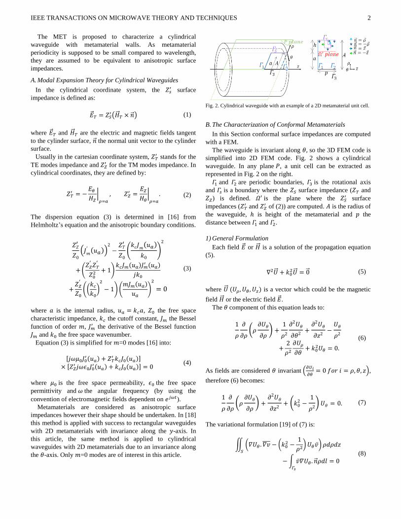
Fig. 2. Cylindrical waveguide with an example of a 2D metamaterial unit cell.

B. The Characterization of Conformal Metamaterials

In this Section conformal surface impedances are computed

with a FEM.

The waveguide is invariant along 𝜃, so the 3D FEM code is

simplified into 2D FEM code. Fig. 2 shows a cylindrical

waveguide. In any plane 𝑃, a unit cell can be extracted as

represented in Fig. 2 on the right.

𝛤1 and 𝛤2 are periodic boundaries, 𝛤3 is the rotational axis

and 𝛤𝑠 is a boundary where the 𝑍𝑆 surface impedance (𝑍𝑇 and

𝑍𝑍) is defined. 𝛺′ is the plane where the 𝑍𝑆′ surface

impedances (𝑍𝑇′ and 𝑍𝑍

′ of (2)) are computed. 𝐴 is the radius of

the waveguide, ℎ is height of the metamaterial and 𝑝 the

distance between 𝛤1 and 𝛤2.

1) General Formulation

Each field �⃗� or �⃗⃗� is a solution of the propagation equation

(5).

∇2�⃗⃗� + 𝑘02�⃗⃗� = 0⃗ (5)

where �⃗⃗� (𝑈𝜌, 𝑈𝜃 , 𝑈𝑧) is a vector which could be the magnetic

field �⃗⃗� or the electric field �⃗� . The 𝜃 component of this equation leads to:

1

𝜌

𝜕

𝜕𝜌(𝜌𝜕𝑈𝜃

𝜕𝜌) +

1

𝜌2

𝜕2𝑈𝜃

𝜕𝜃2+𝜕2𝑈𝜃

𝜕𝑧2−𝑈𝜃

𝜌2

+2

𝜌2𝜕𝑈𝜌

𝜕𝜃+ 𝑘0

2𝑈𝜃 = 0.

(6)

As fields are considered 𝜃 invariant (𝜕𝑈𝑖

𝜕𝜃= 0 𝑓𝑜𝑟 𝑖 = 𝜌, 𝜃, 𝑧),

therefore (6) becomes:

1

𝜌

𝜕

𝜕𝜌(𝜌𝜕𝑈𝜃

𝜕𝜌) +

𝜕2𝑈𝜃

𝜕𝑧2+ (𝑘0

2 −1

𝜌2)𝑈𝜃 = 0. (7)

The variational formulation [19] of (7) is:

∬ (𝛻𝑈𝜃 . 𝛻𝑣̅̅̅̅ − (𝑘0

2 −1

𝜌2)𝑈𝜃�̅�) 𝜌𝑑𝜌𝑑𝑧

𝑆

−∫ �̅�𝛻𝑈𝜃 . �⃗� 𝜌𝑑𝑙

𝛤𝑠

= 0

(8)


3

where 𝑆 is the surface of the unit cell, 𝑣(𝜌, 𝑧) a basis function,

�⃗� the normal unit vector to 𝛤𝑠, where �̅� the 𝑣 conjugate

complex and 𝑑𝑙 the line element along 𝛤𝑠. Along the boundary

𝛤1 and 𝛤2, 𝑈𝜃 is considered as follows:

𝑈𝜃|𝛤2 = 𝑈𝜃|𝛤1 × 𝑒𝑥𝑝(−𝛾𝑧𝑝) (9)

𝛤𝑠 is divided into 𝛤ℎ𝑜𝑟 horizontal walls and 𝛤𝑣𝑒𝑟𝑡 vertical walls.

So:

- for a vertical wall, �⃗� = ±𝑧 :

∇𝑈𝜃 . �⃗� = ±𝜕𝑈𝜃𝜕𝑧

(10)

- for a horizontal wall, �⃗� = ±𝜌 :

∇𝑈𝜃 . �⃗� = ±𝜕𝑈𝜃𝜕𝜌

(11)

(9) and (10) are linked to surface impedances in the following

parts.

2) The Characterization of 𝑍𝑍′

𝑍𝑍′ defined in (2) is generated by 𝐻𝜃 which is considered 𝜃

invariant. 𝐻𝜃 is solution of (8).

The last term of (8) is simplified thanks to (10) and (11):

- for vertical walls:

∇𝐻𝜃 . �⃗� = ±𝜕𝐻𝜃𝜕𝑧

(12)

with Maxwell’s equation and (1):

1

𝑗𝜔𝜖0𝛻 × �⃗⃗� |

𝛤𝑆= 𝑍𝑆 (�⃗⃗� |𝛤𝑆

× (±𝑧 )) (13)

the 𝜌 component of (13) is:

1

𝑗𝜔𝜖0(1

𝜌

𝜕𝐻𝑧𝜕𝜃

−𝜕𝐻𝜃𝜕𝑧

)|𝛤𝑆

= ±𝑍𝑆𝐻𝜃|𝛤𝑆 (14)

due to the 𝜃 invariance, condition (14) becomes:

𝜕𝐻𝜃𝜕𝑧

|𝛤𝑆

= {−𝑗𝜔𝜖0𝑍𝑆𝐻𝜃|𝛤𝑆 𝑖𝑓 �⃗� = 𝑧

𝑗𝜔𝜖0𝑍𝑆𝐻𝜃|𝛤𝑆 𝑖𝑓 �⃗� = −𝑧 (15)

so:

𝛻𝐻𝜃 . �⃗� = −𝑗𝜔𝜖0𝑍𝑠𝐻𝜃|𝛤𝑆 (16)

- for horizontal walls:

∇𝐻𝜃 . �⃗� = ±𝜕𝐻𝜃𝜕𝜌

(17)

with Maxwell’s equation and (1):

1

𝑗𝜔𝜖0𝛻 × �⃗⃗� |

𝛤𝑆= 𝑍𝑆 (�⃗⃗� |𝛤𝑆

× (±𝜌 )) (18)

the 𝑧 component of (18) is:

1

𝑗𝜔𝜖0(1

𝜌 (𝜕(𝜌 𝐻𝜃)

𝜕𝜌−𝜕𝐻𝜌

𝜕𝜃))|

𝛤𝑆

= ∓𝑍𝑆𝐻𝜃|𝛤𝑆 (19)

where 𝜌 = 𝜌ℎ𝑜𝑟 is the horizontal walls radius.

Due to the 𝜃 invariance, condition (19) becomes:

𝜕𝐻𝜃𝜕𝜌

|𝛤𝑆

=

{

(−𝑗𝜔𝜖0𝑍𝑆 −1

𝜌ℎ𝑜𝑟)𝐻𝜃|𝛤𝑆 𝑖𝑓 �⃗� = 𝜌

(𝑗𝜔𝜖0𝑍𝑆 −1

𝜌ℎ𝑜𝑟)𝐻𝜃|𝛤𝑆 𝑖𝑓 �⃗� = −𝜌

(20)

so:

𝛻𝐻𝜃 . �⃗� = (−𝑗𝜔𝜖0𝑍𝑠 −�⃗� . 𝜌

𝜌ℎ𝑜𝑟)𝐻𝜃|𝛤𝑠 (21)

therefore the formulation of (8) with conditions (15) and (20)

is:

∬ (𝛻𝐻𝜃 . 𝛻𝑣̅̅̅̅ − (𝑘0

2 −1

𝜌2)𝐻𝜃�̅�) 𝜌𝑑𝜌𝑑𝑧

𝑆

+ ∑(𝑗𝜔𝜖0𝑍𝑆)∫ �̅�𝐻𝜃𝜌𝑑𝜌

𝛤𝑣𝑒𝑟𝑡𝛤𝑣𝑒𝑟𝑡

+∑(𝑗𝜔𝜖0𝑍𝑆𝜌ℎ𝑜𝑟 + �⃗� . 𝜌 )∫ �̅�𝐻𝜃𝑑𝑧

𝛤ℎ𝑜𝑟𝛤ℎ𝑜𝑟

= 0.

(22)

To solve (22) the linear system (23) is implemented:

𝐴𝐻�⃗⃗� 𝜃 = 0⃗ (23)

where 𝐴𝐻 = [𝐴𝑖𝑗𝐻 ] and �⃗⃗� 𝜃 is defined as follows [20]:

�⃗⃗� 𝜃 = [

𝑢1⋮𝑢𝑁] , 𝐻𝜃 = ∑𝑢𝑗𝛷𝑗

𝑁

𝑗=1

(24)

where 𝑁 is the number of nodes, 𝑢𝑗 is the value of 𝐻𝜃 at the

node 𝑗 in the triangular basis of 𝛷𝑖 and 𝛷𝑖 the basis function of

the vector space. Hence:


4

𝐴𝑖𝑗𝐻 =∬ (𝛻𝛷𝑗. 𝛻𝛷𝑖 − (𝑘0

2 −1

𝜌2)𝛷𝑗𝛷𝑖) 𝜌𝑑𝜌𝑑𝑧

𝑆

+ ∑(𝑗𝜔𝜖0𝑍𝑆)∫ 𝛷𝑖𝛷𝑗𝜌𝑑𝜌


+ ∑(𝑗𝜔𝜖0𝑍𝑆𝜌ℎ𝑜𝑟 + �⃗� . 𝜌 )∫ 𝛷𝑖𝛷𝑗𝑑𝑧


.

(25)

If 𝛤𝑠 is a Perfect Electric Conductor 𝑍𝑆 = 0, (25) becomes:

𝐴𝑖𝑗𝐻 =∬ (𝛻𝛷𝑗. 𝛻𝛷𝑖 − (𝑘0

2 −1


𝑆

+ ∑ �⃗� . 𝜌 ∫ 𝛷𝑖𝛷𝑗𝑑𝑧


(26)

(25) or (26) is solved to obtain 𝐻𝜃 the magnetic field

component (24). The surface impedance in the plane 𝛺′ means

a computation of the electric field component 𝐸𝑧 . From

Maxwell equations:

∇ × �⃗⃗� = 𝑗𝜔𝜖0�⃗� (27)

therefore:

𝐸𝑧|𝛺′

=1

𝑗𝜔𝜖0(𝐻𝜃|𝛺′

𝑎+𝜕𝐻𝜃𝜕𝜌

|𝛺′

) (28)

consequently the surface impedance in 𝛺′ is:

𝑍𝑍′ =

𝐸𝑍𝐻𝜃|𝛺′

=1

𝑗𝜔𝜖0(1

𝑎+

𝜕𝐻𝜃𝜕𝜌

|𝛺′

𝐻𝜃|𝛺′ ) (29)

3) The Characterization of 𝑍𝑇′

𝑍𝑇′ defined in (2) is generated by 𝐸𝜃 which is considered 𝜃

invariant. 𝐸𝜃 is also solution of (8).

The same calculation steps as the Section II.B.2) are carried

out to obtain the formulation for the electric field:

∬ (𝛻𝐸𝜃 . 𝛻𝑣̅̅̅̅ − (𝑘0

2 −1

𝜌2) 𝐸𝜃�̅�) 𝜌𝑑𝜌𝑑𝑧

𝑆

+ ∑ (𝑗𝜔𝜇0𝑍𝑆

)∫ �̅�𝐸𝜃𝜌𝑑𝜌


+∑ (𝑗𝜔𝜇0𝜌ℎ𝑜𝑟

𝑍𝑆+ �⃗� . 𝜌 )∫ �̅�𝐸𝜃𝑑𝑧


= 0.

(30)

To solve (30) the linear system (31) is implemented:

𝐴𝐸�⃗� 𝜃 = 0⃗ (31)

where 𝐴𝐸 = [𝐴𝑖𝑗𝐸 ] and �⃗� 𝜃 is defined as follows:

�⃗� 𝜃 = [

𝑢1⋮𝑢𝑁] , 𝐸𝜃 = ∑𝑢𝑗𝛷𝑗

𝑁

𝑗=1

(32)

where 𝑁 is the number of nodes, 𝑢𝑗 is the value of 𝐸𝜃 at the

node 𝑗 in the triangular basis of 𝛷𝑖 and 𝛷𝑖 the basis function of

the vector space. It follows that:

𝐴𝑖𝑗𝐸 =∬ (𝛻𝛷𝑗. 𝛻𝛷𝑖 − (𝑘0

2 −1


𝑆

+ ∑ (𝑗𝜔𝜇0𝑍𝑆

)∫ 𝛷𝑖𝛷𝑗𝜌𝑑𝜌


+ ∑ (𝑗𝜔𝜇0𝜌ℎ𝑜𝑟

𝑍𝑆+ �⃗� . 𝜌 )∫ 𝛷𝑖𝛷𝑗𝑑𝑧


(33)

when 𝛤𝑠 is a PEC:

𝐸𝜃|𝛤𝑆 = 0 (34)

therefore (33) becomes:

𝐴𝑖𝑗𝐸 =∬ (𝛻𝛷𝑗 . 𝛻𝛷𝑖 − (𝑘0

2 −1


𝑆

= 0 (35)

(33) or (35) is solved to obtain 𝐸𝜃 the electric field

component. The surface impedance in the plane 𝛺′ means a

computation of the magnetic field component 𝐻𝑧. From

Maxwell’s equations:

𝛻 × �⃗� = −𝑗𝜔𝜇0�⃗⃗� (36)

therefore:

𝐻𝑧|𝛺′ =

𝑗

𝜔𝜇0(𝐸𝜃|𝛺′𝑎

+𝜕𝐸𝜃𝜕𝜌

|𝛺′

) (37)

consequently the surface impedance in 𝛺′ is:

𝑍𝑇′ = −

𝐸𝜃𝐻𝑍|𝛺′

= −𝑗𝜔𝜇0

1𝑎+

𝜕𝐸𝜃𝜕𝜌

|𝛺′

𝐸𝜃|𝛺′

(38)

C. The Recursive Solution of Dispersion Equation

The surface impedances (𝑍𝑇′ and 𝑍𝑍

′ ) depend on the

incidence angle [18]. In addition in cylindrical waveguides

this angle should be taken into consideration. Fig. 3 shows the

components of the propagation constants:


5

Fig. 3. Electromagnetic wave propagation in a half-plane (𝜌0𝑧) of the

cylindrical waveguide with the propagation constant components.

𝑘0⃗⃗⃗⃗ = {

𝑘𝜌𝑘𝜃𝑘𝑧

= {𝑘0𝑐𝑜𝑠𝜑0

𝑘0𝑠𝑖𝑛𝜑 (39)

where 𝜑 is the incidence angle.

Hence the 𝜑 angle is deduced from 𝑘𝑧:

𝜑 = 𝑎𝑠𝑖𝑛 (

𝑘𝑧𝑘0) (40)

where 𝑘𝑧 is the phase constant along the 𝑧-axis.

The algorithm in Fig. 4 is implemented to compute the

dispersion diagrams.

The FEM code is necessary to compute the conformal

surface impedances. With this algorithm, different 2D

metamaterials (with 𝜃 invariance) in cylindrical waveguides

can be processed. A 3D FEM code will be required to deal

with 3D metamaterials or modes with angular dependency (𝑚

order different from 0).

Fig. 4. Schematic algorithm to correct the angle 𝜑.

III. RESULTS

In this Section, the method and algorithms are validated in

three different cases:

- firstly the values of the 𝑍𝑆 surface impedance (𝑍𝑇,

𝑍𝑍) is fixed at the 𝐴 radius. Dispersion diagrams of

these waveguides are obtained with the algorithm of

[16]. A comparison is made with dispersion

diagrams computed with the algorithm presented

Fig. 4 and the 𝑍𝑆′ surface impedances (𝑍𝑇

′ , 𝑍𝑍′ )

evaluated for a given 𝑎 radius,

- subsequently the code is applied to a metamaterial: a

corrugation. This result is compared with the result

of [15], to show the improvements made thanks to

the 2D FEM code,

- finally the code is applied to a T-structure

metamaterial.

A. Cylindrical Waveguides with Isotropic and Anisotropic

Surface Impedances

Initially to validate the method, the FEM code is applied for

the fixed (𝑍𝑇, 𝑍𝑍) surface impedances at the 𝐴 radius. The

FEM code computes the (𝑍𝑇′ , 𝑍𝑍

′ ) impedances at another 𝑎

radius. The unit cell is created with the open source software

Gmsh [21] and represented in Fig. 5.

(22) and (30) can be simplified, as there is only one

horizontal wall, therefore 𝐻𝜃 is a solution of:

∬ (𝛻𝐻𝜃 . 𝛻𝑣̅̅̅̅ − (𝑘02 −

1

𝜌2)𝐻𝜃�̅�) 𝜌𝑑𝜌𝑑𝑧

𝑆

+ (𝑗𝜔𝜖0𝑍𝑆𝐴 − 1)∫ 𝐻𝜃�̅�𝑑𝑧

𝛤𝑠

= 0

(41)

𝐸𝜃 is a solution of:

∬ (𝛻𝐸𝜃 . 𝛻𝑣̅̅̅̅ − (𝑘02 −

1

𝜌2) 𝐸𝜃�̅�) 𝜌𝑑𝜌𝑑𝑧

𝑆

+ (𝑗𝜔𝜇0𝐴

𝑍𝑆− 1)∫ 𝐸𝜃�̅�𝑑𝑧

𝛤𝑠

= 0. (42)

The dispersion diagrams obtained for a cylindrical waveguide

of radius A = 30 mm and 𝑎 = 28 mm are illustrated for

various anisotropic surface impedances (curves with dots).

The results are compared with the dispersion diagrams

obtained with the code presented in [16] (curves with circles)

in Fig. 6. The dispersion diagrams are identical hence the

elaborated algorithm is validated.

Fig. 5. Unit cell mesh and dimensions: 𝐴 = 30 mm, 𝑎 = 28 mm, ℎ = 2 mm,

𝑝 = 4 mm.


6

B. A Corrugated Cylindrical Waveguide

A corrugation invariant in 𝜃 direction is now considered.

Fig. 7 presents the corrugated waveguide.

To study this waveguide with HFSS, the same method as

[16] was used. Dispersion diagrams are obtained from the

section represented in Fig. 6 with dashes and using periodic

boundary conditions, see Fig. 8. The propagation constant is

computed thanks to the phase delay between two periodic

boundary conditions and the distance between them. By using

the eigenmode solver in HFSS, the frequency of each solution

is given. The complete dispersion diagram is obtained by

varying the phase delay between the two periodic boundary

conditions from 0° to 180°.

To study this waveguide with the MET, the section of the

waveguide used is extracted in Fig. 7 with dots. Whereas the

structure in HFSS is in 3D, for the MET only a 2D

representation is useful. The unit cell is represented in Fig. 9.

A 2D waveguide section cannot be studied with HFSS. For a

MET validation purpose, a comparison is done with this

software. Since the MET is in 2D and HFSS in 3D, the

computation time is drastically improved anytime with the

MET.

Fig. 7. Corrugated waveguide. The dashed section is the section used in HFSS

and the dotted part is used in the MET.

Fig. 8. Cylindrical representation of a waveguide with periodic boundary

conditions and anisotropic surface simulated in HFSS.

Fig. 6. Dispersion diagrams of a cylindrical waveguide for various anisotropic surface impedances (𝑍𝑇, 𝑍𝑍). The curves with dots are obtained with the code

which computes the (𝑍𝑇′ , 𝑍𝑍

′ ) impedances at a certain distance ℎ (here ℎ = 2 mm) and the curves with circles are obtained with the code based on MET [16].


7

Fig. 9. Unit cell mesh and dimensions: 𝐴 = 100 mm, 𝑎 = 80 mm, ℎ =20 mm, 𝑝 = 26.225 mm, 𝑤 = 20.98 mm and 𝑑 = 18.2 mm.

Fig. 10. Dispersion diagrams of the cylindrical waveguide with the

corrugation presented in Fig. 7 obtained with MET (dots) and HFSS (circles).

For the corrugation 𝛤𝑆 is a PEC hence (24) and (42) are

solved. The dispersion diagrams obtained are compared with

HFSS results in Fig. 10. Both diagrams perfectly coincide with

each other. There is a clear improvement compared to the

dispersion diagram in [15]. Using HFSS the dispersion

diagram is obtained in three days of simulation (Intel (R)

Xeon (R), 1.8 GHz 2 processors, 64 GB of RAM). Using the

MET the dispersion diagram requires a twelve-minute

computation time. Consequently the dispersion diagram is

obtained with the MET around 360 times faster than with

HFSS thanks to the 2D resolution.

C. A T-Structure Metamaterial Waveguide

A T-structure invariant in 𝜃 direction is studied. In Fig. 11

the waveguide is presented. The dashed section represented in

Fig. 11 is extracted and simulated in a 3D FEM code (HFSS)

while the dotted section is inserted in the 2D FEM code in the

MET. The unit cell and the dimensions of this section are

represented in Fig. 12.

Fig. 11. Waveguide with T-structure metamaterial. The dashed section is the

section used in HFSS and the dotted section is used in the MET.

Fig. 12. Unit cell mesh and dimensions: 𝐴 = 50 mm, 𝑎 = 40 mm, ℎ =10 mm, ℎ1 = 2.025 mm, ℎ2 = 6.075 mm, 𝑝 = 13.1125 mm, 𝑝1 =2.6225 mm, and 𝑝2 = 7.8675 mm.

Fig. 13. Dispersion diagrams of the cylindrical waveguide with the T-structure

presented in Fig. 11 obtained with MET (dots) and HFSS (circles).

As in the previous case, 𝛤𝑆 is a PEC, so (24) and (42) are

solved. The dispersion diagrams obtained are compared with

the HFSS result in Fig. 13. The simulation time (Intel (R)

Xeon (R), 1.8 GHz 2 processors, 64 GB of RAM) with the

MET code is 31 minutes compared to the 3D simulation in

HFSS which lasts almost four days.

With this new code it is possible to obtain the dispersion

diagram for 𝑚=0 modes for all kinds of cylindrical

waveguides with 2D metamaterial invariant along the 𝜃-axis.


8

To have the dispersion diagrams with all the modes, the

same algorithm can be used, however another MET code

should be developed using 3D FEM.

IV. CONCLUSION

The Modal Expansion Theory has been developed to

compute the dispersion properties of cylindrical waveguides

with 2D metamaterials for 0 order modes. To demonstrate the

accuracy and the time efficiency of the new method three

different waveguides have been studied: One waveguide with

fixed surface impedances and two with metamaterials which

are invariant in 𝜃 direction. The MET method allows the

characterization of isotropic and anisotropic waveguides

properties whereas HFSS characterizes only isotropic

waveguides. Furthermore all the dispersion diagrams are

obtained in less than a ten-minute computation time while this

process takes more than one hour by using HFSS, as a 3D

Finite Element Method resolution is used in the commercial

software while in the MET it is a 2D FEM resolution.

Consequently the time efficiency of the MET is more relevant

with 2D metamaterials. Indeed for the corrugated waveguide,

the time needed for characterization of propagation properties

is divided by 360 with respect to HFSS. As for the T-structure

waveguide, the time is divided by almost 200.

The more complicated the structure, the more time is saved.

This method is now under development for 3D metamaterials,

to deal with all the mode orders and all other potential

metamaterial structures. Since structures can vary with 𝜃 the

3D FEM code cannot be simplified into 2D FEM code

anymore.

REFERENCES

[1] R. A. Shelby, D. R. Smith and S. Schultz, "Experimental

Verification of a Negative Index of Refraction," Sci., vol.

292, no. 5514, pp. 77-79, Apr. 2001.

[2] D. R. Smith, W. J. Padilla, D. C. Vier, S. C. Nemat-

Nasser, and S. Schultz, "Composite Medium with

Simultaneoustly Negative Permeability and

Permittivity," Phys. Rev. Lett., vol. 84, no. 18, pp. 4184-

4187, May 2000.

[3] V. G. Veselago, "The Electrodynamics of Substances

with Simultaneously Negative Values of ε and µ," Sov.

Phys. Usp., vol. 10, no. 4, pp. 509-514, 1968.

[4] R. W. Ziolkowski and E. Heyman, "Wave Propagation in

Media Having Negative Permittivity and Permeability,"

Phys. Rev. E., vol. 64, no. 5, pp. 1-15, 2001, Art. ID

056625.

[5] Q. Wu, M. D. Gregory, D. H. Werner, P. L. Werner and

E. Lier, "Nature-Inspired Design of Soft, Hard and

Hybrid Metasurfaces," Proc. 2010 IEEE Int. Symp. on

Antennas and Propagation and USNC/URSI National

Radio Science Meeting, Toronto, Canada, July 11-17,

2010, pp. 1-4.

[6] J. G. Pollock and A. K. Iyer, "Below-Cutoff Propagation

in Metamaterial-Lined Circular Waveguides," IEEE

Trans. Microw. Theory Techn., vol. 61, no. 9, pp. 3169-

3178, Sep. 2013.

[7] J. G. Pollock and A. K. Iyer, "Radiation Characteristics

of Miniaturized Metamaterial-Lined Waveguide Probe

Antennas," Proc. 2015 IEEE Int. Symp. on Antennas and

Propagation and USNC/URSI National Radio Science

Meeting, Vancouver, Canada, July 2015.

[8] J. G. Pollock and A. K. Iyer, "Miniaturized Circular-

Waveguide Probe Antennas using Metamaterial Liners,"

IEEE Trans. Antennas Propag., vol. 63, no. 1, pp. 428-

433, Jan. 2015.

[9] J. G. Pollock and A. K. Iyer, "Experimental Verification

of Below-Cutoff Propagation in Miniaturized Circular

Waveguides Using Anisotropic ENNZ Metamaterial

Liners," IEEE Trans. Microw. Theory Techn., vol. 64,

no. 4, pp. 1297-1305, Apr. 2016.

[10] P.-S. Kildal and E. Lier, "Hard Horns Improve Cluster

Feeds of Satellite Antennas,» Electronics Letters, vol. 24,

no. 8, pp. 491-492, Apr. 1988.

[11] R. K. Shaw, E. Lier and C.-C. Hsu., «Profiled Hard

Metamaterial Horns for Multibeam Reflectors," Proc.

2010 IEEE International Symposium on Antennas and

Propagation and USNC/URSI National Radio Science

Meeting, Toronto, Canada, July 11-17, 2010, pp. 1-4.

[12] H. Minnett. and B. Thomas, "A Method of Synthesizing

Radiation Patterns with Axial Symmetry," IEEE Trans.

Antennas Propag., vol. 14, no. 5, pp. 654-656, Sep. 1966.

[13] E. Lier, "Review of Soft and Hard Horn Antennas,

Including Metamaterial-Based Hybrid-Mode Horns,"

IEEE Antennas Propag. Mag., vol. 52, no. 2, pp. 31-39,

Apr. 2010.

[14] B. Byrne, N. Raveu, N. Capet, G. Le Fur and L.

Duchesne, "Reduction of Rectangular Waveguide Cross-

Section with Metamaterials: A New Approach,"

presented at the 9th Int. Congr. on Advanced

Electromagnetic Materials in Microwaves and Optics -

Metamaterials, Oxford, United Kingdom, Sep. 7-12,

2015, pp. 40-42.

[15] B. Byrne, N. Capet and N. Raveu, "Dispersion Properties

of Corrugated Waveguides Based on the Modal Theory,"

in Proc. 8th Eur. Conf. on Antennas Propag., The Hague,

Netherland, Apr. 6-11, 2014, pp.1-3.

[16] N. Raveu, B. Byrne, L. Claudepierre and N. Capet,

"Modal Theory for Waveguides with Anisotropic Surface

Impedance Boundaries," IEEE Trans. Microw. Theory

Techn., vol. 64, no. 4 pp. 1153-1162, Apr. 2016.

[17] B. Byrne, "Etude et Conception de Guides d'Onde et

d'Antennes Cornets à Métamatériaux," These de doctorat

d'état, Univ. Toulouse, Toulouse, 2016.

[18] B. Byrne, N. Raveu, N. Capet, G. Le Fur and L.

Duchesne, "Modal analysis of Rectangular Waveguides

with 2D Metamaterials," Progress In Electromagnetics

Research C, vol. 70, pp. 165-173, 2016.


9

[19] P. Lacoste, "Solution of Maxwell Equation in

Axisymmetric Geometry by Fourier Series

Decomposition and by Use of H(rot) Conforming Finite

Element," Numerische Mathematik, vol. 84, pp. 577-609,

2000.

[20] J.-M. Jin, The Finite Element Method in

Electromagnetics, 3rd ed. Hoboken (New Jersey), USA:

Wiley, 2014.

[21] C. Geuzaine, and J.-F. Remacle "Gmsh: A three-

dimensional finite element mesh generator with built-in

pre- and post-processing facilities," International Journal

for Numerical Methods in Engineering, vol. 79, no. 111,

pp. 1309-1331, 2009.

Lucille Kuhler was born in Metz,

France, in 1992. She received the degree

in electronic engineering and

hyperfrequencies from the Ecole

National d’Aviation Civile (ENAC),

Toulouse, France, in 2016. Currently she

is working toward the Ph. D. degree in

electromagnetism and microwaves at the

University of Toulouse, Toulouse,

France.

Her research topics are electromagnetic wave propagation,

antennas, and metamaterials.

Gwenn Le Fur received the M.S. degree

in signal processing and

telecommunications from the University

of Rennes 1, Rennes, France, in 2006 and

the Ph.D. degree from the Rennes Institute

of Electronics and Telecommunications,

Rennes, France, in 2009.

He was first with the CEA LETI,

Grenoble, France, where he worked on

characterization of small antenna using noninvasive

measurement methods and integrated multi-antenna system.

Then he joined SATIMO Industries (Microwave Vision

Group) as a R&D Engineer. He is now with the Centre

National d’Etudes Spatiales (CNES), Toulouse, France,

working on antenna measurement techniques.

Luc Duchesne got his diploma of

engineer in electronics in 1992 from Ecole

Supérieure d’Electronique de l’Ouest

(ESEO), Angers, France and then a

specialization in aerospace electronics in

1994 from Ecole Nationale Supérieure de

l’Aéronautique et de l’Espace (ISAE –

Supaéro), Toulouse, France.

He started his professional life in 1994 at Deutsche

Aerospace (Dasa) in Munich (now Airbus Defence and Space)

as an Antennas and Payload Components Engineer.

In August 2000, he joined SATIMO close to Paris (Now

Microwave Vision) as Research and Development Director.

From 2000 on to present, he participated to build a strong

R&D department within SATIMO dedicated to the

development of innovative products for the core activity of

antenna measurement systems but also for new activities

concerning non-destructive testing systems and imagery

systems.

He co-authored several conference papers about antennas

and antenna measurement systems. He is also co-inventor of

several patents at DASA and SATIMO.

Nathalie Raveu received the M.S. degree

in electronics and signal processing in

2000 and the Ph. D. degree in 2003.

She is a Professor with the National

Polytechnic Institute of Toulouse (INPT)

and a Research Fellow with the

LAPLACE-CNRS (LAboratory of

PLAsma and Energy Conversion). Her

research topics are oriented toward

development of efficient numerical techniques to address

innovative microwave circuits. During the last years, she has

developed a new method for SICs study, metamaterial horns,

and plasma cavity.

the propagation characteristics of 2-d metamaterial

Documents