The problem of super-replication under constraints

H. Mete Soner

Koc University

Department of Mathematics

Istanbul, Turkey

msoner@ku.edu.tr

Nizar Touzi

Centre de Recherche

en Economie et Statistique

Paris, France

touzi@ensae.fr

January 2002

Abstract

These notes present an overview of the problem of super-replication un-der portfolio constraints. We start by examining the duality approach andits limitations. We then concentrate on the direct approach in the Markovcase which allows to handle general large investor problems and gamma con-straints. In the context of the Black and Scholes model, the main result fromthe practical view-point is the so-called face-lifting phenomenon of the payofffunction.

Key words: Super-replication, duality, dynamic programming, Hamilton-Jacobi-Bellman equation, viscosity solutions.

AMS 1991 subject classifications: Primary 49J20, 60J60; secondary49L20, 35K55.

1

1 Introduction

There is a large literature on the problem of super-replication in finance, i.e. the

minimal initial capital which allows to hedge some given contingent claim at some

terminal time T . Put in a stochastic control terms, the value function of the super-

replication problem is the minimal initial data of some controlled process (the wealth

process) which allows to hit some given target at time T . This stochastic control

problem does not fit in the class of standard problems as presented in the usual

textbooks, see e.g. [13]. This may explain the important attraction that this problem

had on mathematicians.

In its simplest form, this problem is an alternative formulation of the Black and

Scholes theory in terms of a stochastic control problem. The Black and Scholes

solution appears naturally as a (degenerate) dual formulation of the super-replication

problem. However, real financial markets are subject to constraints. The most

popular example is the case of incomplete markets which was studied by Harrisson

and Kreps (1979), and developed further by ElKaroui and Quenez (1995) in the

diffusion case. The effect of the no short-selling constraint has been studied by

Jouini and Kallal (1995). The dual formulation in the general convex constraints

framework has been obtained by Cvitanic and Karatzas (1993) in the diffusion case

and further extended by Follmer and Kramkov (1997) to the general semimartingale

case.

In the general constrained portfolio case, the above-mentioned dual formulation

does not close the problem : except the complete market case, it provides an alter-

native stochastic control problem. The good news is that this problem is formulated

in standard form. But there is still some specific complications since the controls

are valued in unbounded sets. We are then in the context of singular control prob-

lems which typically exhibit a jump in the terminal condition. The main point is to

characterize precisely this face-lifting phenomenon.

However, the duality approach has not been successful to solve more general super-

replication problems. Namely, the dual formulation of the general large investor

problem is still open. The same comment prevails for the super-replication problem

under gamma constraints, i.e. constraints on the unbounded variation part of the

portfolio. We provide a treatment of these problems which avoids the passage from

the dual formulation. The key-point is an original dynamic programming principle

stated directly on the initial formulation of the super-replication problem.

2

Further implications of this new dynamic programming principle are reported in

our accompanying paper [22]. These notes are organized as follows.

Contents

1 Introduction 2

2 Problem formulation 4

2.1 The financial market . . . . . . . . . . . . . . . . . . . . . . . . . . . 4

2.2 Portfolio and wealth process . . . . . . . . . . . . . . . . . . . . . . . 5

2.3 Problem formulation . . . . . . . . . . . . . . . . . . . . . . . . . . . 6

3 Existence of optimal hedging strategies

and dual formulation 8

3.1 Complete market :

the unconstrained Black-Scholes world . . . . . . . . . . . . . . . . . 9

3.2 Optional decomposition theorem . . . . . . . . . . . . . . . . . . . . . 11

3.3 Dual formulation . . . . . . . . . . . . . . . . . . . . . . . . . . . . . 14

3.4 Extensions . . . . . . . . . . . . . . . . . . . . . . . . . . . . . . . . . 16

3.4.1 Simple Large investor models . . . . . . . . . . . . . . . . . . 16

3.4.2 Semimartingale price processes . . . . . . . . . . . . . . . . . 17

4 HJB equation from the dual problem 19

4.1 Dynamic programming equation . . . . . . . . . . . . . . . . . . . . . 19

4.2 Super-solution property . . . . . . . . . . . . . . . . . . . . . . . . . 21

4.3 Subsolution property . . . . . . . . . . . . . . . . . . . . . . . . . . . 23

4.4 Terminal condition . . . . . . . . . . . . . . . . . . . . . . . . . . . . 26

5 Applications 30

3

5.1 The Black-Scholes model with portfolio constraints . . . . . . . . . . 30

5.2 The uncertain volatility model . . . . . . . . . . . . . . . . . . . . . . 30

6 HJB equation from the primal problem

for the general large investor problem 31

6.1 Dynamic programming principle . . . . . . . . . . . . . . . . . . . . . 31

6.2 Supersolution property from DP1 . . . . . . . . . . . . . . . . . . . . 33

6.3 Subsolution property from DP2 . . . . . . . . . . . . . . . . . . . . . 35

7 Hedging under Gamma constraints 37

7.1 Problem formulation . . . . . . . . . . . . . . . . . . . . . . . . . . . 38

7.2 The main result . . . . . . . . . . . . . . . . . . . . . . . . . . . . . . 39

7.3 Discussion . . . . . . . . . . . . . . . . . . . . . . . . . . . . . . . . . 40

7.4 Proof of Theorem 7.1 . . . . . . . . . . . . . . . . . . . . . . . . . . . 41

2 Problem formulation

2.1 The financial market

Given a finite time horizon T > 0, we shall consider throughout these notes a com-

plete probability space (Ω,F , P ) equipped with a standard Brownian motion B =

(B1(t), . . . , Bd(t)), 0 ≤ t ≤ T valued in IRd, and generating the (P−augmentation

of the) filtration IF . We denote by ` the Lebesgue measure on [0, T ].

The financial market consists of a non-risky asset S0 normalized to unity, i.e.

S0 ≡ 1, and d risky assets with price process S = (S1, . . . , Sd) whose dynamics is

defined by a stochastic differential equation. More specifically, given a vector process

µ valued in IRn, and a matrix-valued process σ valued in IRn×n, the price process Si

is defined as the unique strong solution of the stochastic differential equation :

Si(0) = si , dSi(t) = Si(t)

bi(t)dt+d∑

j=1

σij(t)dBj(t)

; (2.1)

here b and σ are assumed to be bounded IF−adapted processes.

4

Remark 2.1 The normalization of the non-risky asset to unity is, as usual, obtained

by discounting, i.e. taking the non-risky asset as a numeraire.

In the financial literature, σ is known as the volatility process. We assume it to

be invertible so that the risk premium process

λ0(t) := σ(t)−1b(t) , 0 ≤ t ≤ T ,

is well-defined. Throughout these notes, we shall make use of the process

Z0(t) = E(−∫ t

0λ0(r)

′dB(r))

:= exp(−∫ t

0λ0(r)

′dB(r)− 1

2

∫ t

0|λ0(r)|2

),

where prime denotes transposition.

Standing Assumption. The volatility process σ satisfies :

E

[exp

1

2

∫ T

0|σ′σ|−1

]< ∞ and sup

[0,T ]|σ′σ|−1 < ∞ P − a.s.

Since b is bounded, this condition ensures that the process λ0 satisfies the Novikov

condition E[exp∫ T0 |λ0|2/2] <∞, and we have E[Z0(T )] = 1. The process Z0 is then

a martingale, and induces the probability measure P0 defined by :

P0(A) := E [Z0(t)1A] for all A ∈ F(t) , 0 ≤ t ≤ T .

Clearly P0 is equivalent to the original probability measure P . By Girsanov’s The-

orem, the process

B0(t) := B(t) +∫ t

0λ0(t)dt , 0 ≤ t ≤ T ,

is a standard Brownian motion under P0.

2.2 Portfolio and wealth process

Let W (t) denote the wealth at time t of some investor on the financial market.

We assume that the investor allocates continuously his wealth between the non-

risky asset and the risky assets. We shall denote by πi(t) the proportion of wealth

invested in the i− th risky asset. This means that

πi(t)W (t) is the amount invested at time t in the i− th risky asset.

5

The remaining proportion of wealth 1−∑di=1 π

i(t) is invested in the non-risky asset.

The self-financing condition states that the variation of the wealth process is only

affected by the variation of the price process. Under this condition, the wealth

process satisfies :

dW (t) = W (t)d∑

i=1

πi(t)dSi(t)

Si(t)

= W (t)π(t)′[b(t)dt+ σ(t)dB(t)] = W (t)π(t)′σ(t)dB0(t) . (2.2)

Hence, the investment strategy π should be restricted so that the above stochastic

differential equation has a well-defined solution. Also π(t) should be based on the

information available at time t. This motivates the following definition.

Definition 2.1 An investment strategy is an IF−adapted process π valued in IRd

and satisfying∫ T0 |σ′π|2(t)dt < ∞ P−a.s.

We shall denote by A the set of all investment strategies.

Clearly, given an initial capital w ≥ 0 together with an investment strategy π, the

stochastic differential equation (2.2) has a unique solution

W πw(t) := wE

(∫ t

0π(r)′σ(r)dB0(r)

), 0 ≤ t ≤ T .

We then have the following trivial, but very important, observation :

W πw is a P0−supermartingale , (2.3)

as a non-negative local martingale under P0.

2.3 Problem formulation

Let K be a closed convex subset of IRd containing the origin, and define the set of

constrained strategies :

AK := π ∈ A : π ∈ K `⊗ P − a.s. .

The set K represents some constraints on the investment strategies.

Example 2.1 Incomplete market : taking K = x ∈ IRd : xi = 0, for some

integer 1 ≤ i ≤ d, means that trading on the i−th risky asset is forbidden.

6

Example 2.2 No short-selling constraint : taking K = x ∈ IRd : xi ≥ 0, for

some integer 1 ≤ i ≤ d, means that the financial market does not allow to sell short

the i−th asset.

Example 2.3 No borrowing constraint : taking K = x ∈ IRd : x1 + . . .+xd ≤ 1means that the financial market does not allow to sell short the non-risky asset or,

in other word, borrowing from the bank is not available.

Now, let G be a non-negative F(T )− measurable random variable. The chief goal

of these notes is to study the following stochastic control problem

V (0) := inf w ∈ IR : W πw(T ) ≥ G P − a.s. for some π ∈ AK . (2.4)

The random variable G is called a contingent claim in the financial mathematics

literature, or a derivative asset in the financial engineering world. Loosely speaking,

this is a contract between two counterparts stipulating that the seller has to pay G

at time T to the buyer. Therefore, V (0) is the minimal initial capital which allows

the seller to face without risk the payment G at time T , by means of some clever

investment strategy on the financial market.

We conclude this section by summarizing the main results which will be presented

in these notes.

1. We start by proving that existence holds for the problem V (0) under very mild

conditions, i.e. there exists a constrained investment strategy π ∈ AK such that

W πV (0)(T )≥G P−a.s. We say that π is an optimal hedging strategy for the contingent

claim G.

The existence of an optimal hedging strategy will be obtained by means of some

representation result which is now known as the optional decomposition theorem

(in the framework of these notes, we can even call it a predictable decomposition

theorem). As a by-product of this existence result, we will obtain a general dual

formulation of the control problem V (0). This will be developed in section 3.

2. In section 4, we seek for more information on the optimal hedging strategy by

focusing on the Markov case. The main result is a characterization of V (0) by

means of a nonlinear partial differential equation (PDE) with appropriate terminal

condition. In some cases, we will be able to solve explicitly the problem. The

solution is typically of the face lifting type, a desirable property from the viewpoint

of the practioners.

7

The derivation of the above-mentioned PDE is obtained from the dual formulation

of V (0) by classical arguments.

3. Section 6 develops the important observation that the same PDE can be ob-

tained by working directly on the original formulation of the problem V (0). Further

developments of this idea will be reported in the accompanying paper [22]. In par-

ticular, such a direct treatment of the problem allows to solve some super-replication

problems for which the dual formulation is not available.

4. The final section of this paper is devoted to the problem of super-replication under

Gamma constraints, for which no dual formulation is available in the literature. The

solution is again of the face lifting type.

3 Existence of optimal hedging strategies

and dual formulation

In this section, we concentrate on the duality approach to the problem of super-

replication under portfolio constraints V (0). Our main objective is to convince the

reader that the presence of constraints does not affect the general methodology of

the proof : the main ingredient is a stochastic representation theorem. We therefore

start by recalling the problem solution in the unconstrained case. This corresponds

to the so-called complete market framework. In the general constrained case, the

proof relies on the same arguments except that : we need to use a more advanced

stochastic representation result, namely the optional decomposition theorem.

Remark 3.1 local martingale representation theorem.

(i) Theorem. Let Y be a local P−local martingale. Then there exits an IRd−valued

process φ such that

Y (t) = Y (0) +∫ t

0φ(r)′dB(r) 0 ≤ t ≤ T and

∫ T

0|φ|2 < ∞ P − a.s.

(see e.g. Dellacherie and Meyer VIII 62).

(ii) We shall frequently need to apply the above theorem to a Q−local martingale Y ,

for some equivalent probability measure Q defined by the density (dQ/dP ) = Z(T )

:= E(−∫ T0 λ(r)′dB(r)

), with Brownian motion BQ := B+

∫ ·0 λ(r)dr. To do this, we

first apply the local martingale representation theorem to theP−local martingale

8

ZY . The result is ZY = Y (0) +∫ ·0 φdB for some adapted process φ with

∫ T0 |φ|2 <

∞. Applying Ito’s lemma, one can easily check that we have :

Y (t) = Y (0) +∫ t

0ψ(r)′dBQ(r) 0 ≤ t ≤ T where ψ := Z−1φ+ λY .

Since Z and Y are continuous processes on the compact interval [0, T ], it is imme-

diately checked that∫ T0 |ψ|2 < ∞ Q−a.s.

3.1 Complete market :

the unconstrained Black-Scholes world

In this paragraph, we consider the unconstrained case K = IRd. The following result

shows that V (0) is obtained by the same rule than in the celebrated Black-Scholes

model, which was first developed in the case of constant coefficients µ and σ.

Theorem 3.1 Assume that G > 0 P−a.s. Then :

(i) V (0) = E0[G]

(ii) if E0[G] < ∞, then W πV (0)(T ) = G P−a.s. for some π ∈ A.

Proof. 1. Set F := w ∈ IR : W πw(T ) ≥ G for some π ∈ A. From the

P0−supermartingale property of the wealth process (2.3), it follows that w ≥ E0[G]

for all w ∈ F . This proves that V (0) ≥ E0[G]. Observe that this concludes the

proof of (i) in the case E0[G] = +∞.

2. We then concentrate on the case E0[G] <∞. Define

Y (t) := E0[G|F(t)] for 0 ≤ t ≤ T .

Apply the local martingale representation theorem to the P0−martingale Y , see

Remark 3.1. This provides

Y (t) = Y (0) +∫ t

0ψ(r)′dB0(r) for some process ψ with

∫ T

0|ψ|2 <∞ .

Now set π := (Y σ′)−1ψ. Since Y is a positive continuous process, it follows from

Standing Assumption that π ∈ A, and Y = Y (0)E (∫ ·0 π(r)∗σ(r)dB0(r)) = W π

Y (0).

The statement of the theorem follows from the observation that Y (T ) = G. 2

9

Remark 3.2 Statement (ii) in the above theorem implies that existence holds for

the control problem V (0), i.e. there exists an optimal trading strategy. But it

provides a further information, namely that the optimal hedging strategy allows to

attain the contingent claim G. Hence, in the unconstrained setting, all (positive)

contingent claims are attainable. This is the reason for calling this financial market

complete.

Remark 3.3 The proof of Theorem 3.1 suggests that the optimal hedging strategy

π is such that the P0− martingale Y has the stochastic representation Y = E[G] +∫ ·0 Y π

′σdB0. In the Markov case, we have Y (t) = v(t, S(t)). Assuming that v is

smooth, it follows from an easy application of Ito’s lemma that

∆i(t) :=πi(t)W π

V (0)(t)

Si(t)=

∂v

∂si(t, S(t)) .

We now focus on the positivity condition in the statement of Theorem 3.1, which

rules out the main example of contingent claims, namely European call options

[Si(T )−K]+, and European put options [K − Si(T )]+. Indeed, since the portfolio

process is defined in terms of proportion of wealth, the implied wealth process is

strictly positive. Then, it is clear that such contingent claims can not be attained,

in the sense of Remark 3.2, and there is no hope for Claim (ii) of Theorem 3.1 to

hold in this context. However, we have the following easy consequence.

Corollary 3.1 Let G be a non-negative contingent claim. Then

(i) For all ε > 0, there exists an investment strategy πε ∈ A such that W πε

V (0)(T ) =

G+ ε.

(ii) V (0) = E0[G].

Proof. Statement (i) follows from the application of Theorem 3.1 to the contingent

claim G+ ε. Now let Vε(0) denote the value of the super-replication problem for the

contingent claim G + ε. Clearly, V (0) ≤ Vε(0) = E0[G + ε], and therefore V (0) ≤E0[G] by sending ε to zero. The reverse inequality holds since Part 1 of the proof

of Theorem 3.1 does not require the positivity of G. 2

Remark 3.4 In the Markov setting of Remark 3.3 above, and assuming that v is

smooth, the approximate optimal hedging strategy of Corollary 3.1 (i) is given by

∆iε(t) :=

πiε(t)W

πVε(0)(t)

Si(t)=

∂

∂siv(t, S(t)) + ε =

∂v

∂si(t, S(t)) ;

10

observe that ∆ := ∆ε is independent of ε.

Example 3.1 The Black and Scholes formula : consider a financial market with

a single risky asset d = 1, and let µ and σ be constant coefficients, so that the

P0−distribution of ln [S(T )/S(t)], conditionally on F(t), is gaussian with mean

−σ2(T − t)/2 and variance σ2(T − t). As a contingent claim, we consider the

example of a European call option, i.e. G = [S(T ) − K]+ for some exercise price

K > 0. Then, one can compute directly that :

V (t) = v(t, S(t)) where v(t, s) := sF (d(t, s))−KF(d(t, s)− σ

√T − t

),

d(t, s) := (σ√T − t)−1 ln(K−1s) +

1

2σ√T − t ,

and F (x) = (2π)−1/2∫ x−∞ e

−u2/2du is the cumulative function of the gaussian distri-

bution. According to Remark 3.3, the optimal hedging strategy in terms of number

of shares is given by :

∆(t) = F (d(t, S(t))) .

3.2 Optional decomposition theorem

We now turn to the general constrained case. The key-point in the proof of The-

orem 3.1 was the representation of the P0−martingale Y as a stochastic integral

with respect to B0; the integrand in this representation was then identified to the

investment strategy. In the constrained case, the investment strategy needs to be

valued in the closed convex set K, which is not guaranteed by the representation

theorem. We then need to use a more advanced representation theorem. The results

of this section were first obtained by ElKaroui and Quenez (1995) for the incomplete

market case, and further extended by Cvitanic and Karatzas (1993).

We first need to introduce some notations. Let

δ(y) := supx∈K

x′y

be the support function of the closed convex set K. Since K contains the origin, δ

is non-negative. We shall denote by

K := dom(K) = y ∈ IRd : δ(y) <∞

the effective domain of δ. For later use, observe that K is a closed convex cone of

IRd. Recall also that, since K is closed and convex, we have the following classical

11

result from convex analysis (see e.g. Rockafellar 1970) :

x ∈ K if and only if δ(y)− x′y ≥ 0 for all y ∈ K , (3.1)

x ∈ ri(K) if and only if x ∈ K and infy∈K1

(δ(y)− x′y) > 0 , (3.2)

where

K1 := K ∩ y ∈ IRd : |y| = 1 and δ(y) + δ(−y) 6= 0 .

We next denote by D the collection of all bounded adapted processes valued in K.

For each ν ∈ D, we set

βν(t) := exp(−∫ t

0δ(ν(r))dr

), 0 ≤ t ≤ T ,

and we introduce the Doleans-Dade exponential

Zν(t) := E(−∫ t

0λν(r)

′dB(r))

where λν := σ−1(b− ν) = λ0 − σ−1ν .

Since b and ν are bounded, λν inherits the Novikov condition E[exp

(12

∫ T0 |λν |2

)]<

∞ from Standing Assumption. We then introduce the family of probability measures

Pν(A) := E [Zν(t)1A] for all A ∈ F(t) , 0 ≤ t ≤ T .

Clearly Pν is equivalent to the original probability measure P . By Girsanov Theo-

rem, the process

Bν(t) := B(t) +∫ t

0λν(r)dr = B0(t)−

∫ t

0σ(r)−1ν(r)dr , 0 ≤ t ≤ T , (3.3)

is a standard Brownian motion under Pν .

Remark 3.5 The reason for introducing these objects is that the important prop-

erty (2.3) extends to the family D :

βνWπw is a Pν−supermartingale for all ν ∈ D, π ∈ AK , (3.4)

and w > 0. Indeed, by Ito’s lemma together with (3.3),

d(W πwβν) = W π

wβν [−(δ(ν)− π′ν)dt+ π′σdBν ] .

In view of (3.1), this shows that W πwβν is a non-negative local Pν−supermartingale,

which provides (3.4).

12

Theorem 3.2 Let Y be an IF− adapted positive cadlag process. Assume that

the process βνY is a Pν−supermartingale for all ν ∈ D.

Then, there exists a predictable non-decreasing process C, with C(0) = 0, and a

constrained portfolio π ∈ AK such that Y = W πY (0) − C.

Proof. We start by applying the Doob (unique) decomposition theorem (see e.g.

Dellacherie and Meyer VII 12) to the P0−supermartingale Y β0 = Y , together with

the local martingle representation theorem, under the probability measure P0. This

implies the existence of an adapted process ψ0 and a non-decreasing predictable

process C0 satisfying C0(0) = 0,∫ T0 |ψ0|2 <∞, and :

Y (t) = Y (0) +∫ t

0ψ0(r)dB0(r)− C0(t) , (3.5)

see Remark 3.1. Observe that

M0 := Y (0) +∫ ·

0ψ0dB0 = Y + C0 ≥ Y > 0 . (3.6)

We then define

π0 := M−10 (σ′)−1ψ0 .

From Standing Assumption together with the continuity of M0 on [0, T ] and the

fact that∫ T0 |ψ0|2 < ∞, it follows that π0 ∈ A. Then M0 = W π

Y (0) and by (3.6),

Y = W π0

Y (0) − C0 .

In order to conclude the proof, it remains to show that the process π is valued in K.

2. By Ito’s lemma together with (3.3), it follows that :

d(Y βν) = M0βνπ′0σdBν − βν [(Y δ(ν)−M0π

′0ν)dt+ dC0] .

This provides the unique decomposition of the Pν−supermartingale Y βν = Mν +Cν ,

with

Mν := Y (0) +∫ ·

0M0βνπ

′0σdBν and Cν :=

∫ ·

0βν [(Y δ(ν)−M0π

′0ν)dt+ dC0] ,

into a Pν−local martingale Mν and a predictable non-decreasing process Cν starting

from the origin. We conclude from this that :

0 ≤∫ t

0β−1

ν dCν = C0(t) +∫ t

0(Y δ(ν)−M0π

′0ν) (r)dr

≤ C0(t) +∫ t

0M0 (δ(ν)− π′0ν) (r)dr for all ν ∈ D , (3.7)

13

where the last inequality follows from (3.6) and the non-negativity of the support

function δ.

3. Now fix some ν ∈ D, and define the set Fν := (t, ω) : [π′0ν + δ(ν)](t, ω) < 0.Consider the process

ν(n) = ν1F cy

+ nν1Fy , n ∈ IN .

Clearly, since K is a cone, we have ν(n) ∈ D for all n ∈ IN . Writing (3.7) with ν(n),

we see that, whenever ` ⊗ P [Fν ] > 0, the left hand-side term converges to −∞ as

n→∞, a contradiction. Hence `⊗P [Fν ] = 0 for all ν ∈ D. From (3.1), this proves

that π ∈ K `⊗ P−a.s. 2

3.3 Dual formulation

Let T be the collection of all stopping times valued in [0, T ], and define the family

of random variables :

Yτ := esssupν∈D Eν [Gγν(τ, T )|F(τ)] ; τ ∈ T where γν(τ, T ) :=βν(T )

βν(τ),

and Eν [·] denotes the conditional expectation operator under Pν . The purpose of

this section is to prove that V (0) = Y0, and that existence holds for the control

problem V (0). As a by-product, we will also see that existence for the control

problem Y0 holds only in very specific situations. These results are stated precisely

in Theorem 3.3. As a main ingredient, their proof requires the following (classical)

dynamic programming principle.

Lemma 3.1 (Dynamic Programming). Let τ ≤ θ be two stopping times in T .

Then :

Yτ = esssupν∈D Eν [Yθγν(τ, θ)|F(τ)] .

Proof. 1. Conditioning by F(θ), we see that

Yτ ≤ esssupν∈D Eν [γν(τ, θ)Eν [Gγν(θ, T )|F(θ)]] ≤ esssupν∈D Eν [γν(τ, θ)Yθ] .

2. To see that the reverse inequality holds, fix any µ ∈ D, and let Dτ,θ(µ) be the

subset of D whose elements coincide with µ on the stochastic interval [[τ, µ]]. Let

(νk)k be a maximizing sequence of Yθ, i.e.

Yθ = limk→∞

Jνk(θ) where Jν(θ) := Eν [Gγν(θ, T )|F(θ)] ;

14

the existence of such a sequence follows from the fact that the family Jν(θ), ν ∈ Dis directed upward. Also, since Jν(θ) depends on ν only through its realization on

the stochastic interval [θ, T ], we can assume that νk ∈ Dτ,θ(µ). We now compute

that

Yτ ≥ Eνk[Gγνk

(τ, T )|F(τ)] = Eµ [γµ(τ, θ)Jνk(θ)|F(τ)] ,

which implies that Yτ ≥ Eµ [γµ(τ, θ)Yθ|F(τ)] by Fatou’s lemma. 2

Now, observe that we may take the stopping times τ in the definition of the family

Yτ , τ ∈ T to be deterministic and thereby obtain a non-negative adapted process

Y (t), 0 ≤ t ≤ T. A natural question is whether this process is consistent with the

family Yτ , τ ∈ T in the sense that Yτ (ω) = Y (τ(ω)) for a.e. ω ∈ Ω. For general

control problems, this is a delicate issue. However, in our context, it follows from

the above dynamic programming principle that the family Yτ , τ ∈ T satisfies a

supermartingale property :

E [βν(θ)Yθ|F(τ)] ≤ βν(τ)Yτ for all τ, θ ∈ T with τ ≤ θ .

By a classical argument, this allows to extract a process Y out of this family, which

satisfies the supermartingale property in the usual sense. We only state precisely

this technical point, and send the interested reader to Karatzas and Shreve (1999)

Appendix D or Cvitanic and Karatzas (1993), Proposition 6.3.

Corollary 3.2 There exists a cadlag process Y = Y (t), 0 ≤ t ≤ T, consistent

with the family Yτ , τ ∈ T , and such that Y βν is a Pν−supermartingale for all

ν ∈ D.

We are now able for the main result of this section.

Theorem 3.3 Assume that G > 0 P−a.s. Then :

(i) V (0) = Y (0),

(ii) if Y (0) < ∞, existence holds for the problem V (0), i.e. W πV (0)(T ) ≥ G P−a.s.

for some π ∈ AK,

(iii) existence holds for the problem Y (0) if and only if

W πV (0)(T ) = G and βνW

πV (0) is a Pν−martingale

for some pair (π, ν) ∈ AK ×D.

15

Proof. 1. We concentrate on the proof of Y (0) ≥ V (0) as the reverse inequality is

a direct consequence of (3.4). The process Y , extracted from the family Yτ , τ ∈ T in Corollary 3.2, satisfies Condition (i) of the optional decomposition theorem 3.2.

Then Y = W πY (0) −C for some constrained portfolio π ∈ AK , and some predictable

non-decreasing process C with C(0) = 0. In particular, W πY (0)(T ) ≥ Y (T ) = G.

This proves that Y (0) ≥ V (0), completing the proof of (i) and (ii).

2. It remains to prove (iii). Suppose thatW πV (0)(T ) =G and βνW

πV (0) is a Pν−martin-

gale for some pair (π, ν) ∈ AK × D. Then, by the first part of this proof, Y (0) =

V (0) = Eν

[W π

V (0)(T )βν(T )]

= Eν [Gβν(T )], i.e. ν is a solution of Y (0).

Conversely, assume that Y (0) = Eν [Gβν(T )] for some ν ∈ D. Let π be the

solution of V (0), whose existence is established in the first part of this proof. By

definition W πV (0)(T ) − G ≥ 0. Since βνW

πV (0) is a Pν−super-martingale, it follows

that Eν

[βν(W

πV (0)(T )−G)

]≤ 0. This proves that W π

V (0)(T ) − G = 0 P−a.s. We

finally see that the Pν−super-martingale βνWπV (0) has constant Pν−expectation :

Y (0) ≥ Eν

[βν(t)W

πV (0)(t)

]≥ Eν

[Eν

(βν(T )W π

V (0)(T )∣∣∣F(t)

)]= Eν [βν(T )G] = Y (0) ,

and therefore βνWπV (0) is a Pν−martingale. 2

3.4 Extensions

The results of this section can be extended in many directions.

3.4.1 Simple Large investor models

Suppose that the drift coefficient of the price process depends on the investor’s

strategy, so that the price dynamics are influenced by the action of the investor.

More precisely, the price dynamics ar defined by :

Si(0) = si , dSi(t) = Si(t)

bi(t, S(t), π(t))dt+d∑

j=1

σij(t)dBj(t)

, (3.8)

where b(t, s, ·) is convex and non-negative. Define the Legendre-Fenchel transform :

b(t, s, y) := supx∈K

(bi(t, ω, x) + x′y

)for y ∈ IRd ,

together with the associated effective domain :

K(t, s) :=y ∈ IRd : b(t, s, y) <∞

.

16

Next, we introduce the set D consisting of all bounded adapted processes ν satisfying

ν(t) ∈ K(t, S(t)) `⊗ P−a.s.

For any process ν ∈ D, define the equivalent probability measure Pν by the density

process

Zν(t) := E(∫ t

0[σ(t)−1ν(t)]′dW (t)

),

and the discount process :

βν(t) := exp(−∫ t

0b(r, S(r), ν(r))dr

).

Then, the results of the previous section can be extended to this context by defining

the dynamic version of the dual problem

Yτ := esssupν∈DEν [Gγν(τ, T )| F(τ)] ; τ ∈ T where γν(τ, T ) :=βν(T )

βν(τ).

Important observation : in the above simple large investor model, only the drift

coefficient in the dynamics of S is influenced by the portfolio π. Unfortunately,

the analysis developed in the previous paragraphs does not extend to the general

large investor problem, where the volatility process is influenced by the action of the

investor. This is due to the fact that there is no way to get rid of the dependence of

σ on π by proceeding to some equivalent change of measure : it is well-known that

the measures induced by diffusions with different diffusion coefficients are singular.

In section 6, the general large investor problem will be solved by an alternative

technique.

Remark 3.6 From an economic viewpoint, one may argue that the dynamics of the

price process should be influenced by the variation of the portfolio holdings of the

investor d[πW ]. This is related to the problem of hedging under gamma constraints.

The last section of these notes presents some preliminary results in this direction.

3.4.2 Semimartingale price processes

All the results of the previous sections extend to the case where the price process S

is defined as a semimartingale valued in (0,∞)d. Let us state the generalization of

Theorem 3.3; we refer the interested reader to Follmer and Kramkov (1997) for a

deep analysis.

17

the wealth process is defined by

W πw(t) := E

(∫ t

0π(r)′diag[S(r)]−1dS(r)

),

where diag[s] denotes the diagonal matrix with diagonal components si, and the set

of admissible portfolio AK is the collection of all predictable processes π valued in

K for which the above stochastic integral is well-defined.

Let P be the collection of all probability measures Q ∼ P such that :

W π1 e

−C is a Q−local supermartingale for all π ∈ A , (3.9)

for some increasing predictable process C (depending on Q). An increasing pre-

dictable process CQ is called an upper variation process under Q if it satisfies (3.9)

and is minimal with respect to this property. Such a process is shown to exist.

Then, the results of the previous sections can be extended to this context by

defining the dynamic version of the dual problem

Yτ := esssupQ∈PEQ [GγQ(τ, T )| F(τ)] ; τ ∈ T , γQ(τ, T ) := eCQ(τ)−CQ(T ) ,

where EQ denotes the expectation operator under Q.

The main ingredient for this result is an extension of the optional decomposition

result of Theorem 3.2. Observe that the non-decreasing process C in this more

general framework is optional, and not necessarily predictable. We recall that

- the optional tribe is generated by Ft−adapted processes with cd-lag trajecto-

ries;

- a process X is optional if the map (t, ω) 7−→ X(t, ω) is measurable with respect

to the optional tribe;

- the predictable tribe is generated by Ft−−adapted processes with left-continuous

trajectories;

- a process X is predictable if the map (t, ω) 7−→ X(t, ω) is measurable with respect

to the predictable tribe.

18

4 HJB equation from the dual problem

4.1 Dynamic programming equation

In order to characterize further the solution of the super-replication problem, we

now focus on the Markov case :

b(t) = b(t, S(t)) and σ(t) = σ(t, S(t)) ,

where b and σ are now vector and matrix valued functions defined on [0, T ]×IRd. In

order to guarantee existence of a strong solution to the SDE defining S, we assume

that b and σ are Lipschitz functions in the s variable, uniformly in t. We also

consider the special case of European contingent claim :

G = g (S(T )) ,

where g is a map from [0,∞)d into IR+. We first extend the definition of the dual

problem in order to allow for a moving time origin :

v(t, s) := supν∈D

E [g (St,s(T )) γν(t, T )] = supν∈D

E[g (St,s(T )) e−

∫ T

tδ(ν(r))dr

].

Here, St,s denotes the unique strong solution of (2.1) with initial data St,s(t) = s.

Notice that, although the control process ν is path dependent, the value function

of the above control problem v(t, s) is a function of the current values of the state

variables. This is a consequence of the important results of Haussman (1985) and

ElKaroui, Nguyen and Jeanblanc (1986).

Let v∗ and v∗ be respectively the lower and upper semi-continuous envelopes of

v :

v∗(t, s) := lim inf(t′,s′)→(t,s)

v(t′, s′) and v∗(t, s) := lim sup(t′,s′)→(t,s)

v(t′, s′) .

We shall frequently appeal to the infinitesimal generator of the process S under P0 :

Lϕ := ϕt +1

2Trace

[diag[s]σσ′diag[s]D2ϕ

],

where diag[s] denotes the diagonal matrix with diagonal components si, the t sub-

script denotes the partial derivative with respect to the t variable, Dϕ is the gradient

vector with respect to s, and D2ϕ is the Hessian matrix with respect to s. We will

also make use of the first order differential operator :

Hyϕ := δ(y)ϕ− y′diag[s]Dϕ for y ∈ K .

19

An important role will be played by the following face-lifted payoff function

g(s) := supy∈K

g(sey)e−δ(y) for s ∈ IRd+ , (4.1)

where sey is the IRd vector with components sieyi. We finally recall from (3.2) the

notation K1 := K ∩ |y| = 1 and δ(y) + δ(−y) 6= 0, and we denote by

xK the orthogonal projection of x on vect(K) ,

where vect(K) is the vector space generated by K. The main result of this section

is the following.

Theorem 4.1 Let σ be bounded and suppose that v is locally bounded. Assume fur-

ther that g is lower semi-continuous, g is upper semi-continuous with linear growth.

Then :

(i) For all (t, x) ∈ [0, T )× IRd and y ∈ K, the function r 7−→ δ(y)r− ln (v(t, ex+ry))

is non decreasing; in particular, v(t, ex) = v(t, exK ) for all (t, x) ∈ [0, T )× IRd,

(ii) v is a (discontinuous) viscosity solution of

min

−Lv , inf

y∈K1

Hyv

= 0 on [0, T )× (0,∞)d , v(T, ·) = g . (4.2)

The proof of the above statement is a direct consequence of Propositions 4.1, 4.2,

4.4, 4.5, and Corollary 4.1, reported in the following paragraphs.

We conclude this paragraph by recalling the notion of discontinuous viscosity

solutions. The interested reader can find an overview of this theory in [5] or [13].

Given a real-valued function u, we shall denote by u∗ and u∗ its lower and the upper

semi-continuous envelopes. We also denote by §n the set of all n × n symmetric

matrices with real coefficients.

Definition 4.1 Let F be a map from IRn× IRn×Sn into IR, O an open domain of

IRn, and consider the non-linear PDE

F(x, u(x), Du(x), D2u(x)

)= 0 for x ∈ O . (4.3)

Assume further that F (x, r, p, A) is non-increasing in A (in the sense of symmetric

matrices). Let u : O −→ IR be a locally bounded function.

20

(i) We say that u is a (discontinuous) viscosity supersolution of (4.3) if for any

x0 ∈ O and ϕ ∈ C2(O) satisfying

(u∗ − ϕ)(x0) = minx∈O

(u∗ − ϕ) ,

we have

F ∗(x0, u∗(x0), Dϕ(x0), D

2ϕ(x0))≥ 0 .

(ii) We say that u is a (discontinuous) viscosity subsolution of (4.3) if for any x0 ∈ Oand ϕ ∈ C2(O) satisfying

(u∗ − ϕ)(x0) = maxx∈O

(u∗ − ϕ) ,

we have

F∗(x0, u

∗(x0), Dϕ(x0), D2ϕ(x0)

)≤ 0 .

(iii) We say that u is a (discontinuous) viscosity solution of (4.3) if it satisfies the

above requirements (i) and (ii).

In these notes the map F defining the PDE (4.3) will always be continuous. In

the accompanying paper [22], the case where F is not continuous will be frequently

met.

4.2 Super-solution property

We first start by proving that v∗ is a viscosity super-solution of the HJB equation

(4.2).

Proposition 4.1 Suppose that the value function v is locally bounded. Then v is a

(discontinuous) viscosity super-solution of the PDE

min

−Lv∗ , inf

y∈KHyv∗

(t, s) ≥ 0 . (4.4)

Proof. Let (t, s) be fixed in [0, T ) × IRd+, and consider a smooth test function ϕ,

mapping [0, T ]× IRd+ into IR, and satisfying

0 = (v∗ − ϕ)(t, s) = min[0,T ]×IRd

+

(v∗ − ϕ) . (4.5)

21

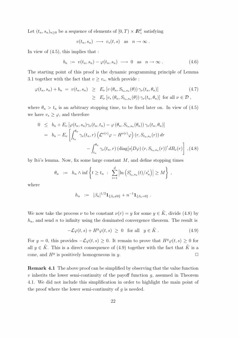
Let (tn, sn)n≥0 be a sequence of elements of [0, T )× IRd+ satisfying

v(tn, sn) −→ v∗(t, s) as n→∞ .

In view of (4.5), this implies that :

bn := v(tn, sn)− ϕ(tn, sn) −→ 0 as n→∞ . (4.6)

The starting point of this proof is the dynamic programming principle of Lemma

3.1 together with the fact that v ≥ v∗, which provide :

ϕ(tn, sn) + bn = v(tn, sn) ≥ Eν [v (θn, Stn,sn(θ)) γν(tn, θn)] (4.7)

≥ Eν [v∗ (θn, Stn,sn(θ)) γν(tn, θn)] for all ν ∈ D ,

where θn > tn is an arbitrary stopping time, to be fixed later on. In view of (4.5)

we have v∗ ≥ ϕ, and therefore

0 ≤ bn + Eν [ϕ(tn, sn)γν(tn, tn)− ϕ (θn, Stn,sn(θn)) γν(tn, θn)]

= bn − Eν

[∫ θn

tnγν(tn, r)

(Lν(r)ϕ−Hν(r)ϕ

)(r, Stn,sn(r)) dr

−∫ θn

tnγν(tn, r) (diag[s]Dϕ) (r, Stn,sn(r))′ dBν(r)

],(4.8)

by Ito’s lemma. Now, fix some large constant M , and define stopping times

θn := hn ∧ inf

t ≥ tn :

d∑i=1

∣∣∣ln (Sitn,sn

(t)/sin

)∣∣∣ ≥M

,

where

hn := |βn|1/21βn 6=0 + n−11βn=0 .

We now take the process ν to be constant ν(r) = y for some y ∈ K, divide (4.8) by

hn, and send n to infinity using the dominated convergence theorem. The result is

−Lϕ(t, s) +Hyϕ(t, s) ≥ 0 for all y ∈ K . (4.9)

For y = 0, this provides −Lϕ(t, s) ≥ 0. It remain to prove that Hyϕ(t, s) ≥ 0 for

all y ∈ K. This is a direct consequence of (4.9) together with the fact that K is a

cone, and Hy is positively homogeneous in y. 2

Remark 4.1 The above proof can be simplified by observing that the value function

v inherits the lower semi-continuity of the payoff function g, assumed in Theorem

4.1. We did not include this simplification in order to highlight the main point of

the proof where the lower semi-continuity of g is needed.

22

We are now in a position to prove statement (i) of Theorem 4.1.

Corollary 4.1 Suppose that the value function v is locally bounded. For fixed

(t, x) ∈ [0, T )× IRd and y ∈ K, consider the function

hy : r 7−→ δ(y)r − ln(v∗(t, e

x+ry)).

Then

(i) hy is non-decreasing;

(ii) v∗(t, ex) = v∗(t, e

xK ), where xK := projvect(K)(x) is the orthogonal projection of

x on the vector space generated by K;

(iii) assuming further that g is lower semi-continuous, we have v(t, ex) = v(t, exK ).

Proof. (i) From Proposition 4.1, function v∗ is a viscosity supersolution of

Hyv∗ = δ(y)v − y′diag[s]Dv∗ ≥ 0 for all y ∈ K .

Consider the change of variable w(t, x) := ln[v∗(t, e

x1, . . . , exd

)]exp (−δ(y)t). Then

w is a viscosity supersolution of the equation −wx ≥ 0, and therefore w is non-

increasing. This completes the proof.

(ii) We first observe that vect(K)⊥ ⊂ K and δ(y) = 0 for all y ∈ vect(K)⊥. Now,

since y := x− xK ∈ vect(K)⊥, it follows from (i) that

− ln v∗(t, exK ) = hy(1) ≥ hy(0) = − ln v∗(t, e

x)

= h−y(0) ≥ h−y(−1) = − ln v∗(t, exK ) .

Now, assuming further that g is lower semi-continuous, it follows from a simple

application of Fatou’s lemma that v is lower semicontinuous, and (iii) is just a re-

statement of (ii). 2

4.3 Subsolution property

The purpose of this paragraph is to prove that the value function v is a (discon-

tinuous) viscosity subsolution of the HJB equation (4.4). Since it has been shown

in Proposition 4.1 that v is a supersolution of this PDE, this will prove that v is a

(discontinuous) viscosity solution of the HJB equation (4.4).

23

Proposition 4.2 Assume that the payoff function g is lower semi-continuous, and

the value function v is locally bounded. Then, v is a (discontinuous) viscosity sub-

solution of the PDE

min

−Lv∗ , inf

y∈K1

Hyv∗

≤ 0 . (4.10)

Proof. Let ϕ : [0, T ]× IRd −→ IR be a smooth function and (t0, s0) ∈ [0, T )× IRd

be such that :

0 = (v∗ − ϕ)(t0, s0) > (v∗ − ϕ)(t, s) for all (t, s) 6= (t0, s0) , (4.11)

i.e. (t0, s0) is a strict global maximizer of (v∗−ϕ) on [0, T )× IRd. Since v∗ > 0 and

v∗(t, ex) = v∗(t, exK ) by Corollary 4.1, we may assume that ϕ > 0 and ϕ(t, ex) =

ϕ(t, exK ) as well. Observe that this is equivalent to

diag[s](Dϕ/ϕ)(t, s) ∈ vect(K) for all (t, s) ∈ [0, T )× (0,∞)d . (4.12)

In order to prove the required result we shall assume that :

−Lϕ(t0, s0) > 0 and infy∈K1

Hyϕ(t0, s0) > 0 . (4.13)

In view of (4.12), the second inequality in (4.13) is equivalent to

diag[s0] (Dϕ/ϕ) (t0, s0) ∈ ri(K) . (4.14)

Our final goal will be to end up with a contradiction of the dynamic programming

principle of Lemma 3.1.

1. By smoothness of the test function ϕ, it follows from (4.13)-(4.14) that one can

find some parameter δ > 0 such that

−Lϕ(t, s) ≥ 0 and diag[s] (Dϕ/ϕ) (t, s) ∈ K (4.15)

for all (t, s) ∈ D := (t0 − δ, t0 + δ)× (s0eδB) , (4.16)

where B is the unit closed ball of IR1 and s0eδB is the collection of all points ξ in

IRd such that | ln(ξi/si0)| < δ for i = 1, . . . , d. We also set

max∂D

(v∗

ϕ

)=: e−2β < 1 , (4.17)

where strict inequality follows from (4.11).

24

Next, let (tn, sn)n be a sequence in D such that :

(tn, sn) −→ (t, s) and v(tn, sn) −→ v∗(t, s) . (4.18)

Using the fact that v ≤ v∗ together with the smoothness of ϕ, we may assume that

the sequence (tn, sn)n satisfies the additional requirement

v(tn, sn) ≥ e−βϕ(tn, sn) . (4.19)

For ease of notation, we denote Sn(·) := Stn,sn(·), and we introduce the stopping

times

θn := infr ≥ tn : (r, Sn(r)) 6∈ D .

Observe that, by continuity of the process Sn,

(θn, Sn(θn)) ∈ ∂D so that v∗ (θn, Sn(θn)) ≤ e−2βϕ (θn, Sn(θn)) , (4.20)

as a consequence of (4.17).

2. Let ν be any control process in D. Since v ≤ v∗, it follows from (4.19) and (4.20)

that :

v (θn, Sn(θn)) γν(tn, θn)− v(tn, sn) ≤ e−2β(1− eβ

)ϕ(tn, sn)

+e−2β (ϕ (θn, Sn(θn)) γν(tn, θn)− ϕ(tn, sn)) .

We now apply Ito’s lemma, and use the definition of θn together with (4.15). The

result is :

v (θn, Sn(θn)) γν(tn, θn)− v(tn, sn) = e−2β(1− eβ

)ϕ(tn, sn)

+e−2β∫ θn

tnγν(tn, r)(−Hν(r) + L)ϕ(r, Sn(r))dr

+e−2β∫ θn

tnγν(tn, r)(Dϕ

′diag[s]σ)(r, Sn(r))dBν(r)

≤ e−2β(1− eβ

)ϕ(tn, sn)

+e−2β∫ θn

tn(Dϕ′diag[s]σ)(r, Sn(r))dBν(r) .

We finally take expected values under Pν , and use the arbitrariness of ν ∈ D to see

that :

v(tn, sn) ≤ supν∈D

Eν [v (θn, Sn(θn)) γν(tn, θn)|F(tn)] + e−2β(1− eβ

)ϕ(tn, sn)

< supν∈D

Eν [v (θn, Sn(θn)) γν(tn, θn)|F(tn)] ,

which is in contradiction with the dynamic programming principle of Lemma 3.1.

2

25

4.4 Terminal condition

From the definition of the value function v, we have :

v(T, s) = g(s) for all s ∈ IRd+ .

However, we are facing a singular stochastic control problem, as the controls ν are

valued in an unbounded set. Typically this situation induces a jump in the terminal

condition so that we only have :

v∗(T, s) ≥ v(T, s) = g(s) .

The main difficulty is then to characterize the terminal condition of interest v∗(T, ·).The purpose of this section is to prove that v∗(T, ·) is related to the function g

defined in 4.1.

We first start by deriving the PDE satisfied by v∗(T, ·), as inherited from Propo-

sition 4.1.

Proposition 4.3 Suppose that g is lower semi-continuous and v is locally bounded.

Then v∗(T, ·) is a viscosity super-solution of

min

v∗ − g , inf

y∈KHyv∗

(T, ·) .

Proof. 1. We first check that v∗(T, ·) ≥ g. Let (tn, sn)n be a sequence of [0, T ) ×(0,∞)d converging to (T, s), and satisfying v(tn, sn) −→ v∗(T, s). Since δ(0) = 0, it

follows from the definition of v that

v(tn, sn) ≥ E0 [g (Stn,sn(T ))] .

Since g ≥ 0, we may apply Fatou’s lemma, and derive the required inequality using

the lower semi-continuity condition on g, together with the continuity of St,s(T ) in

(t, s).

2. It remains to prove that v∗(T, ·) is a viscosity super-solution of

Hyv∗(T, ·) ≥ 0 for all y ∈ K . (4.21)

Let f ≤ v∗(T, ·) be a C2 function satisfying, for some s0 ∈ (0,∞)d,

0 = (v∗(T, ·)− f)(s0) = minIRd

+

(v∗(T, ·)− f) .

26

Since v∗ is lower semi-continuous, we have v∗(T, s0) = lim inf(t,s)→(T,s0) v∗(t, s), and

v∗(Tn, sn) −→ v∗(T, s0) for some sequence (Tn, sn) −→ (T, s0) .

Define

ϕn(t, s) := f(s)− 1

2|s− s0|2 +

T − t

T − Tn

,

let B = s ∈ IRd+ :

∑i | ln (si/si

0)| ≤ 1, and choose (tn, sn) such that :

(v∗ − ϕn)(tn, sn) = min[Tn,T ]×B

(v∗ − ϕn) .

We shall prove the following claims :

tn < T for large n , (4.22)

sn −→ s0 along some subsequence, and v∗(tn, sn) −→ v∗(T, s0) . (4.23)

Admitting this, wee see that, for sufficiently large n, (tn, sn) is a local minimizer of

the difference (v∗ − ϕn). Then, the viscosity super-solution property, established in

Proposition 4.1, holds at (tn, sn), implying that Hyv∗(tn, sn) ≥ 0, i.e.

δ(y)v∗(tn, sn)− y′diag[s] (Df(sn)− (sn − s0)) ≥ 0 for all y ∈ K1 ,

by definition of ϕn in terms of f . In view of (4.23), this provides the required

inequality (4.21).

Proof of (4.22) : Observe that for all s ∈ B,

(v∗ − ϕn)(T, s) = v∗(T, s)− f(s) +1

2|s− s0|2 ≥ v∗(T, s)− f(s) ≥ 0 .

Then, the required result follows from the fact that :

limn→∞

(v∗ − ϕn)(Tn, sn) = limn→∞

v∗(Tn, sn)− f(sn) +

1

2|sn − s0|2 −

1

T − Tn

= −∞ .

Proof of (4.23) : Since (sn)n is valued in the compact subset B, we have sn −→ s

along some subsequence, for some s ∈ B. We now use respectively the following

facts : s0 minimizes the difference v∗(T, ·) − f , v∗ is lower semi-continuous, sn −→s0, tn ≥ Tn, and (tn, sn) minimizes the difference v∗−ϕn on [Tn, T ]× B. The result

is :

0 ≤ (v∗(T, ·)− f)(s)− (v∗(T, ·)− f)(s0)

27

≤ lim infn→∞

(v∗ − ϕn)(tn, sn)− 1

2|sn − s0|2

−(v∗ − ϕn)(Tn, sn) +1

2|sn − s0|2 −

tn − Tn

T − Tn

≤ −1

2|s− s0|2 + lim inf

n→∞(v∗ − ϕn)(tn, sn)− (v∗ − ϕn)(Tn, sn)

≤ −1

2|s− s0|2 + lim sup

n→∞(v∗ − ϕn)(tn, sn)− (v∗ − ϕn)(Tn, sn)

≤ −1

2|s− s0|2 ≤ 0 ,

so that all above inequalities hold with equality, and (4.23) follows. 2

We are now able to characterize a precise bound on the terminal condition of the

singular stochastic control problem v(t, s).

Proposition 4.4 Suppose that g is lower semi-continuous and v is locally bounded.

Then v∗(T, ·) ≥ g.

Proof. We first change variables by setting F (x) := ln [v∗(T, ex)], with ex :=

(ex1, . . . , exd

)′. From Proposition 4.3, it follows that F satisfies :

δ(y)− y′DF ≥ 0 for all y ∈ K .

Introducing the lower semi-continuous function h(t) := F (x+ ty)− δ(y)t, for fixed

x ∈ IRd and y ∈ K, we see that h is a viscosity super-solution of the equation

−h′ ≥ 0. By classical result in the theory of viscosity solutions, we conclude that

h is non-increasing. In particular h(0) ≥ h(1), i.e. F (x) ≥ F (x + y) − δ(y) for all

x ∈ IRd and y ∈ K, and

F (x) ≥ supy∈K

F (x+ y)− δ(y)

≥ supy∈K

lng(ex+y

)e−δ(y)

for all x ∈ IRd .

This provides the required result by simply turning back to the initial variables. 2

We now intend to provide the reverse inequality of Proposition 4.4. In order

to simplify the presentation, we shall provide an easy proof which requires strong

assumptions.

Proposition 4.5 Let σ be a bounded function, and g be an upper semi-continuous

function with linear growth. Suppose that v is locally bounded. Then v∗(T, ·) ≤ g.

28

Proof. Suppose to the contrary that V ∗(T, s)− g(s) =: 2η > 0 for some s ∈ (0,∞)d.

Let (Tn, sn) be a sequence in [0, T ]× (0,∞)d satisfying :

(Tn, sn) −→ (T, s) , V (Tn, sn) −→ V ∗(T, s)

and

V (Tn, sn) > g(s) + η for all n ≥ 1 .

From the (dual) definition of V , this shows the existence of a sequence (νn)n in Dsuch that :

E0Tn,sn

[g(S

(n)T e

∫ T

Tnνn

r dr)e−∫ T

Tnδ(νn

r )dr]> g(s) + η for all n ≥ 1 , (4.24)

where

S(n)T := snE

(∫ T

Tn

σ(t, Sνn

t )dWt

).

We now use the sublinearity of δ to see that :

E0Tn,sn

[g(S

(n)T e

∫ T

Tnνn

r dr)e−∫ T

Tnδ(νn

r )dr]

≤ E0Tn,sn

[g(S

(n)T e

∫ T

Tnνn

r dr)e−δ(∫ T

Tnνn

r dr)]

≤ E0Tn,sn

[g(S

(n)T

)],

where we also used the definition of g together with the fact that K is a closed

convex cone of IRd. Plugging this inequality in (4.24), we see that

g(s) + η ≤ E0tn,sn

[g(S

(n)T

)]. (4.25)

By easy computation, it follows from the linear growth condition on g that

E0∣∣∣g(S(n)

T )∣∣∣2 ≤ Const

(1 + e(T−t)‖σ‖2∞

).

This shows that the sequenceg(S

(n)T ), n ≥ 1

is bounded in L2(P 0), and is there-

fore uniformly integrable. We can therefore pass to the limit in (4.25) by means of

the dominated convergence theorem. The required contradiction follows from the

upper semi-continuity of g together with the a.s. continuity of ST in the initial data

(t, s). 2

29

5 Applications

5.1 The Black-Scholes model with portfolio constraints

In this paragraph we report an explicit solution of the super-replication problem

under portfolio constraints in the context of the Black-Scholes model. This result

was obtained by Broadie, Cvitanic and Soner (1997).

Proposition 5.1 Let d = 1, σ(t, s) = σ > 0, and consider a lower semi-continuous

payoff function g : IR+ −→ IR. Assume that the face-lifted payoff function g is

upper semi-continuous and has linear growth. Then :

v(t, s) = E0 [g (St,s(T ))] ,

i.e. v(t, s) is the unconstrained Black-and Scholes price of the face-lifted contingent

claim g (St,s(T )).

Proof. By a direct application of Theorem 4.1, the value function v(t, s) solves the

PDE (4.2). When σ is constant, it follows from the maximum principle that the

PDE (4.2) reduces to :

−Lv = 0 on [0, T )× (0,∞)d , v(T, ·) = g ,

and the required result follows from the Feynman-Kac representation formula. 2

5.2 The uncertain volatility model

In this paragraph, we study the simplest incomplete market model. The number of

risky assets is now d = 2. We consider the case K = IR×0 so that the second risky

asset is not tradable. In order to satisfy the conditions of Theorem 4.1, we assume

that the contingent claim is defined by G = g(S1(T )), where the payoff function

g : IR+ −→ IR+ is continuous and has polynomial growth. We finally introduce the

notations :

σ(t, s1) := sups2>0

[σ211 + σ2

12](t, s1, s2) and σ(t, s1) := infs2>0

[σ211 + σ2

12](t, s1, s2)

We report the following result from Cvitanic, Pham and Touzi (1999) which follows

from Theorem 4.1. We leave its verification for the reader.

30

Proposition 5.2 (i) Assume that σ < ∞ on [0, T ] × IR+. Then v(t, s) = v(t, s1)

solves the Black-Scholes-Barrenblatt equation

−vt −1

2

[σ2v+

s1s1− σ2v−s1s1

]= 0, on [0, T )× (0,∞), v(T, s1) = g(s1) for s1 > 0.

(ii) Assume that σ = ∞ and

either g is convex or σ = 0 .

Then v(t, s) = gconc(s1), where gconc is the concave envelope of g.

6 HJB equation from the primal problem

for the general large investor problem

In this section, we present an original dynamic programming principle stated di-

rectly on the initial formulation of the super-replication problem. We then prove

that the HJB equation of Theorem 4.1 can be obtained by means of this dynamic

programming principle. Hence, if one is only interested in the derivation of the HJB

equation, then the dual formulation is not needed any more.

An interesting feature of the analysis of this section is that it can be extended

to problems where the dual formulation is not available. A first example is the

large investor problem with feedback of the investor’s portfolio on the price process

through the drift and the volatility coefficients; see section 3.4.1. This problem is

treated in the present section and does not present any particular difficulty. Another

example is the problem of super-replication under gamma constraints which will be

discussed in the last section of these notes. In an accompanying paper, the analysis

of this section will be further extended to cover front propagation problems related

to the theory of differential geometry.

6.1 Dynamic programming principle

In this section, the price process S is defined by the controlled stochastic differential

equation :

Sπt,s(t) = s

dSπt,s(r) = diag[Sπ

t,s](r)[b(r, Sπ

t,s(r), π(r))dr + σ(r, Sπt,s(r), π(r))dB(r)

],

31

where b : [0, T ]× IRd ×K −→ IRd and σ : [0, T ]× IRd ×K −→ IRd×d are bounded

functions, Lipschitz in the s variable uniformly in (t, π).

The wealth process is defined by

W πt,s,w(t) = w

dW πt,s,w(r) = W π

t,s,w(r)π(r)′[b(r, Sπ

t,s(r), π(r))dr + σ(r, Sπt,s(r), π(r))dB(r)

].

Given a European contingent claim G = g(St,s(T )) ≥ 0, the super-replication prob-

lem is defined by

v(t, s) := infw > 0 : W π

t,s,w(T ) ≥ g(Sπ

t,s(T ))P − a.s. for some π ∈ AK

.

The main result of this section is the following.

Lemma 6.1 Let (t, s) ∈ [0, T )×(0,∞)d be fixed, and consider an arbitrary stopping

time θ valued in [t, T ]. Then,

v(t, s) = infw > 0 : W π

t,s,w(θ) ≥ v(θ, Sπ

t,s(θ))P − a.s. for some π ∈ AK

.

In order to derive the HJB equation by means of the above dynamic programming

principle, we shall write it in the following equivalent form :

DP1 Let (t, s) ∈ [0, T ) × (0,∞)d, (w, π) ∈ (0,∞) × AK be such that W πt,s,w(T ) ≥

g(Sπ

t,s(T ))P−a.s. Then

W πt,s,w(θ) ≥ v

(θ, Sπ

t,s(θ))

P − a.s.

DP2 Let (t, s) ∈ [0, T )× (0,∞)d, and set w := v(t, s). then for all stopping time θ

valued in [t, T ],

P[W π

t,s,w−η(θ) > v(θ, Sπ

t,s(θ))]

< 1 for all η > 0 and π ∈ AK .

Idea of the proof. The proof of DP1 follows from the trivial observation that

Sπt,s(T ) = Sπ

θ,Sπt,s(θ)

(T ) and W πt,s,w(T ) = W π

θ,St,s(θ),Wt,s,w(θ)(T ) .

The proof of DP2 is more technical, we only outline the main idea. Let θ be some

stopping time valued in [t, T ], and suppose that

W := W πt,s,w−η(θ) > v

(θ, Sπ

t,s(θ))

P − a.s. for some η > 0 and π ∈ AK .

32

Set S := Sπt,s(θ). By definition of the super-replication problem v

(θ, S

)starting at

time θ, there exists an admissible portfolio π ∈ AK such that

W πθ,S,W

(T ) ≥ g(Sπ

θ,S(T )

)P − a.s.

This is the delicate place of this proof, as one has to appeal to a measurable selection

argument in order to define the portfolio π. In order to complete the proof, it suffices

to define the admissible portfolio π := π1[t,θ) + π1[[θ,T ], and to observe that :

W πt,s,w−η(T ) = W π

θ,S,W(T ) ≥ g

(Sπ

θ,S(T )

)= g

(Sπ

t,s(T ))

P − a.s.

which is in contradiction with the definition of w. 2

6.2 Supersolution property from DP1

In this paragraph, we prove the following result.

Proposition 6.1 Suppose that the value function v is locally bounded, and the con-

straint set K is compact. Then v is a discontinuous viscosity supersolution of the

PDE

min

−Lv∗ , inf

y∈KHyv∗

(t, s) ≥ 0

where

Lu := ut(t, s) +1

2Tr[diag[s]σσ′(t, s, α)diag[s]D2u(t, s)

]α := diag[s]

Du

u(t, s) .

The compactness condition on the constraints setK is assumed in order to simplify

the proof. In the case of a small investor model (b and σ do not depend on π),

the following argument is an alternative proof of Proposition 4.1 which uses part

DP1 of the above direct dynamic programming principle of Lemma 6.1, instead

of the classical dynamic programming principle of Lemma 3.1 stated on the dual

formulation of the problem. Recall that such a dual formulation is not available in

the context of a general large investor model with σ depending on π.

Proof. Let (t, s) be fixed in [0, T ) × IRd+, and consider a smooth test function ϕ,

mapping [0, T ]× IRd+ into (0,∞), and satisfying

0 = (v∗ − ϕ)(t, s) = min[0,T ]×IRd

+

(v∗ − ϕ) . (6.1)

33

Let (tn, sn)n≥0 be a sequence of elements of [0, T )× IRd+ satisfying

v(tn, sn) −→ v∗(t, s) as n→∞ .

We now set

wn := v(tn, sn) + maxn−1 , 2|v(tn, sn)− ϕ(tn, sn)| for all n ≥ 0 ,

and observe that

cn := lnwn − lnϕ(tn, sn) > 0 and cn −→ 0 as n→∞ , (6.2)

in view of (6.1). Since wn > v(tn, sn), it follows from DP1 that :

lnv(θn, S

πntn,sn

(θn))

≤ lnW πn

tn,sn,wn(θn)

for some πn ∈ AK ,

where, for each n ≥ 0, θn is an arbitrary stopping time valued in [tn, T ], to be chosen

later on. In the rest of this proof, we simply denote (Sn,Wn) :=(Sπn

tn,sn,W πn

tn,sn,wn

).

By definition of the test function ϕ, we have v ≥ v∗ ≥ ϕ, and therefore :

0 ≤ cn + lnϕ(tn, sn)− lnϕ (θn, Sn(θn))

+∫ θn

tn

[π′nb−

1

2|σ′πn|2

](r, Sn(r), πn(r)) dr

+∫ θn

tn(π′nσ) (r, Sn(r), πn(r)) dB(r) .

Applying Ito’s lemma to the smooth test function lnϕ, we see that :

0 ≤ cn +∫ θn

tn(πn − hn)′σ (r, Sn(r), πn(r)) dB(r) (6.3)

−∫ θn

tn

[Lπn(r)ϕ

ϕ− (πn − hn)′b+

|σ′hn|2 − |σ′πn|2

2

](r, Sn(r), πn(r)) dr ,

where we introduced the additional notations

hn(r) := diag[Sn(r)]Dϕ

ϕ(r, Sn(r)) ,

and

Lαϕ(t, s) := ϕt(t, s) +1

2Trdiag[s]σσ′(t, s, α)diag[s]D2ϕ(t, s)

.

2. Given a positive integer k, we define the equivalent probability measure P kn by :

dP kn

dP

∣∣∣∣∣F(tn)

:= E(∫ T

tnσ−1

[−b+ k

πn − hn

|πn − hn|1πn−hn 6=0

](r, Sn(r)) dB(r)

);

34

recall that σ−1 and b are bounded functions. Taking expected values in (6.3) under

P kn , conditionally on F(tn), we see that :

0 ≤ cn − Ek

∫ θn

tn

[Lπn(r)ϕ

ϕ+ k|πn − hn|+

|σ′hn|2 − |σ′πn|2

2

](r, Sn(r), πn(r)) dr ,

where Ek denote the conditional expectation operator under P kn . We now devide by

√cn and send n to infinity to get :

0 ≤ lim infn

Ek

∫ θn

tn

[−Lπn(r)ϕ

ϕ− k|πn − hn| −

|σ′hn|2 − |σ′πn|2

2

](r, Sn(r), πn(r)) dr ,

(6.4)

3. We now fix the stopping times :

θn :=√cn ∧ inf

r ≥ tn : Sn(r) 6∈ sne

γB,

for some constant γ, where B is the unit closed ball of IR1 and sneδB is the collection

of all points ξ in IRd such that | ln (ξi/sin)| ≤ γ. Then, by dominated convergence,

it follows from (6.4) that :

0 ≤ infα∈K

−Lαϕ

ϕ− k

∣∣∣∣∣α− diag[s]Dϕ

ϕ(t, s)

∣∣∣∣∣+ 1

2

∣∣∣∣∣σ′diag[s]Dϕ

ϕ(t, s)

∣∣∣∣∣2

− |σ′α|2 .

Since K is compact, the above minimum is attained at some αk ∈ K, and αk −→α ∈ K along some subsequence. Sending k to infinity, we see that one must have

α = diag[s]Dϕ

ϕ(t, s) ∈ K and −Lαϕ ≥ 0 .

2

6.3 Subsolution property from DP2

We now show that part DP2 of the dynamic programming principle stated in Lemma

6.1 allows to prove an extension of the subsolution property of Proposition 4.2 in

the general large investor model. To simplify the presentation, we shall only work

out the proof in the case where K has non-empty interior; the general case can

be addressed by the same argument as in section 4.3, i.e. by first deducing, from

the supersolution property, that v(t, ex) depends only on the projection xK of x on

aff(K) = vect(K).

35

Proposition 6.2 Suppose that the value function v is locally bounded, and the con-

straints set K has non-empty interior. Then, v is a discontinuous viscosity subso-

lution of the PDE

min

−Lv∗ , inf

y∈K1

Hyv∗

(t, s) ≥ 0

Proof. 1. In order to simplify the presentation, we shall pass to the log-variables.

Set x := lnw, Xπt,s,x := lnW π

t,s,w, and u := ln v. By Ito’s lemma, the controlled

process Xπ is given by :

Xπt,s,x(τ) = x+

∫ τ

t

(π′b− 1

2|σ′π|2

) (r, Sπ

t,s(r), π(r))dr

+∫ τ

t(π′σ)

(r, Sπ

t,s(r), π(r))dB(r) . (6.5)

With this change of variable, Proposition 6.2 states that u∗ satisfies on [0, T ) ×(0,∞)d the equation :

min

−Gu∗ , inf

y∈K1

(δ(y)− diag[s]Du∗(t, s))

≤ 0

in the viscosity sense, where

Gu∗(t, s) := u∗t (t, s) +1

2|σ′(t, s, α)diag[s]Du∗(t, s)|2

+1

2Tr[diag[s]σσ′(t, s, α)diag[s]D2u∗(t, s)

],

and α := diag[s]Du∗(t, s) .

2. We argue by contradiction. Let (t0, s0) ∈ [0, T ) × (0,∞)d and a C2 ϕ(t, s) be

such that :

0 = (w∗ − ϕ)(t0, s0) > (w∗ − ϕ)(t, s) for all (t, s) 6= (t0, s0) ,

and suppose that

Gϕ(t, s) > 0 and diag[s0]Dϕ(t0, s0) ∈ int(K) .

Set π(t, s) := diag[s]Dϕ(t, s). Let 0 < α < T − t0 be an arbitrary scalar and define

the neighborhood of (t0, s0) :

N :=(t, s) ∈ (t0 − α, t0 + α)× s0e

αB : π(t, s) ∈ K and − Gϕ(t, s) ≥ 0,

36

where B is again the unit closed ball of IR1 and s0eαB is the collection of all points

ξ ∈ IRd such that | ln (ξi/si0)| ≤ γ. Since (t0, s0) is a strict maximizer of (u∗ − ϕ),

observe that :

−4β := max∂N

(u∗ − ϕ) < 0 .

3. Let (t1, s1) be some element in N such that :

x1 := u(t1, s1) ≥ u∗(t0, s0)− β = ϕ(t0, s0)− β ≥ ϕ(t1, s1)− 2β ,

and consider the controlled process

(S, X) :=(Sπ

t1,s1, lnW π

t1,s1,w1e−β

)with feedback control π(r) := π

(r, S(r)

),

which is well-defined at least up to the stopping time

θ := infr > t0 :

(r, S(r)

)6∈ N

.

Observe that u ≤ u∗ ≤ ϕ − 3β on ∂N by continuity of the process S. We then

compute that :

x1 − β − u(θ, S(θ)

)≥ u(t1, s1)− 3β − ϕ

(θ, S(θ)

)≥ β + ϕ(t1, s1)− ϕ

(θ, S(θ)

). (6.6)

4. From the definition of π, the diffusion term of the difference dX(r)− dϕ(r, S(r))

vanishes up to the stopping time θ. It then follows from (6.6), Ito’s lemma, and

(6.5) that

X(θ)− u(θ, S(θ)

)≥ β +

∫ θ

t1dX(r)− dϕ(r, S(r))

= β +∫ θ

t1Gϕ(r, S(r))

≥ β > 0 P − a.s.

where the last inequality follows from the definition of the stopping time θ and the

neighborhood N . This proves that W πt1,s1,w1e−β > v(θ, Sπ

t1,s1(θ) P−a.s., which is the

required contradiction to DP2. 2

7 Hedging under Gamma constraints

In this section, we focus on an alternative constraint on the portfolio π. Let Y :=

diag[S(t)]−1π(t)W (t) denote the vector of number of shares of the risky assets held

37

at each time. By definition of the portfolio strategy, the investor has to adjust his

strategy at each time t, by passing the number of shares from Y (t) to Y (t+dt). His

demand in risky assets at time t is then given by ”dY (t)”.

In an equilibrium model, the price process of the risky assets would be pushed

upward for a large demand of the investor. We therefore study the hedging problem

with constrained portfolio adjustment. This problem turns out to present serious

mathematical difficulties. The analysis of this section is reported from [19], and

provides a solution of the problem in a very specific situation. We hope that this

presentation will encourage some readers to attack some of the possible extensions.

7.1 Problem formulation

We consider a financial market which consists of one bank account, with constant

price process S0(t) = 1 for all t ∈ [0, T ], and one risky asset with price process

evolving according to the Black-Scholes model :

St,s(u) := sE (σ(B(t)−B(u)) , t ≤ u ≤ T.

Here B is a standard Brownian motion in IR defined on a complete probability space

(Ω,F , P ). We shall denote by IF = F(t), 0 ≤ t ≤ T the P -augmentation of the

filtration generated by B.

Observe that there is no loss of generality in taking S as a martingale, as one

can always reduce the model to this case by judicious change of measure (P0 in

the previous sections). On the other hand, the subsequent analysis can be easily

extended to the case of a varying volatility coefficient.

We denote by Y = Y (u), t ≤ u ≤ T the process of number of shares of risky

asset S held by the agent during the time interval [t, T ]. Then, by the self-financing

condition, the wealth process induced by some initial capital w and portfolio strategy

Y is given by :

W (u) = w +∫ u

tY (r)dSt,s(r), t ≤ u ≤ T.

In order to introduce constraints on the variations of the hedging portfolio Y , we

restrict Y to the class of continuous semimartingales with respect to the filtration

IF . Since IF is the Brownian filtration, we define the controlled portfolio strategy

Y α,γt,s,y by :

Y α,γt,y (u) = y +

∫ u

tα(r)dr + +

∫ u

tγ(r)σdB(r), t ≤ u ≤ T, (7.1)

38

where y ∈ IR is the initial portfolio and the control pair (α, γ) takes values in

Bt := (L∞([t, T ]× Ω ; `⊗ P ) )2 .

Hence a trading strategy is defined by the triple (y, α, γ) with y ∈ IR and (α, γ) ∈Bt. The associated wealth process, denoted by Wα,γ

t,w,s,y, is given by :

W α,γt,w,s,y(u) = w +

∫ u

tY α,γ

t,y (r)dSt,s(r), t ≤ u ≤ T . (7.2)

We now formulate the Gamma constraint in the following way. Let Γ be a constant

fixed throughout the paper. Given some initial capital w > 0, we define the set of

w-admissible trading strategies by :

At,s(w) :=(y, α, γ) ∈ IR× Bt : γ(.) ≤ Γ and Wα,γ

t,w,s,y(.) ≥ 0.

As in the previous sections, We consider the super-replication problem of some

European type contingent claim g(St,s(T )) :

v(t, s) := infw : Wα,γ

t,w,s,y(T ) ≥ g(St,s(T )) a.s. for some (y, α, γ) ∈ At,s(w).

(7.3)

7.2 The main result

Our goal is to derive the following explicit solution : v(t, s) is the (unconstrained)

Black-Scholes price of some convenient face-lifted contingent claim g(St,s(T )), where

the function g is defined by

g(s) := hconc(s) + Γs ln s with h(s) := g(s)− Γs ln s ,

and hconc denotes the concave envelope of h. Observe that this function can be

computed easily. The reason for introducing this function is the following.

Lemma 7.1 g is the smallest function satisfying the conditions

(i) g ≥ g , and (ii) s 7−→ g(s)− s ln s is concave.

The proof of this easy result is omitted.

Theorem 7.1 Let g be a non-negative lower semi-continuous mapping on IR+. As-

sume further that

s 7−→ g(s)− C s ln s is convex for some constant C . (7.4)

Then the value function (7.3) is given by :

v(t, s) = E [g (St,s(T ))] for all (t, s) ∈ [0, T )× (0,∞) .

39

7.3 Discussion

1. We first make some comments on the model. Formally, we expect the optimal

hedging portfolio to satisfy

Y (u) = vs(u, St,s(u)) ,

where v is the minimal super-replication cost; see Section 3.1. Assuming enough

regularity, it follows from Ito’s lemma that

dY (u) = A(u)du+ σ(u, St,s(u))St,s(u)vss(u, St,s(u))dB(u) ,

where A(u) is given in terms of derivatives of v. Compare this equation with (7.1)

to conclude that the associated gamma is

γ(u) = St,s(u) vss(u, St,s(u)) .

Therefore the bound on the process γ translates to a bound on svss. Notice that, by

changing the definition of the process γ in (7.1), we may bound vss instead of svss.

However, we choose to study svss because it is a dimensionless quantity, i.e., if all

the parameters in the problem are increased by the same factor, svss still remains

unchanged.

2. Observe that we only require an upper bound on the control γ. The similar

problem with a lower bound on γ is still open, and presents some specific difficulties.

In particular, it seems that the control∫ t0 α(r)dr has to be relaxed to the class of

bounded variation processes...

3. The extension of the analysis of this section to the multi-asset framework is also

an open problem. The main point is the extension of Lemma 7.5 below.

4. Intuitively, we expect to obtain a similar type solution to the case of portfolio

constraints. If the Black-Scholes solution happens to satisfy the gamma constraint,

then it solves the problem with gamma constraint. In this case v satisfies the PDE

−Lv = 0. Since the Black-Scholes solution does not satisfy the gamma constraint,

in general, we expect that function v solves the variational inequality :

min −Lv,Γ− svss = 0 . (7.5)

5. An important feature of the log-normal Black and Sholes model is that the

variational inequality (7.5) reduces to the Black-Scholes PDE −Lv = 0 as long

40

as the terminal condition satisfies the gamma constraint (in a weak sense). From

Lemma 7.1, the face-lifted payoff function g is precisely the minimal function above

g which satisfies the gamma constraint (in a weak sense). This explains the nature

of the solution reported in Theorem 7.1, namely v(t, s) is the Black-Scholes price of

the contingent claim g (St,s(T )).

6. One can easily check formally that the variational inequality (7.5) is the HJB

equation associated to the stochastic control problem :

v(t, s) := supν∈N

E

[g(Sν

t,s(T ))− 1

2

∫ T

tν(t)[Sν

t,s(r)]2dr

],

where N is the set of all non-negative, bounded, and IF− adapted processes, and :

Sνt,s(u) := E

(∫ u

t[σ2 + ν(r)]1/2dB(r)

), for t ≤ u ≤ T .

The above stochastic control problem is a candidate for some dual formulation of

the problem v(t, s) defined in (7.3). Observe, however, that the dual variables ν are

acting on the diffusion coefficient of the controlled process Sν , so that the change of

measure techniques of Section 3 do not help to prove the duality connection between

v and v.

A direct proof of some duality connection between v and v is again an open

problem. In order to obtain the PDE characterization (7.5) of v, we shall make use

of the dynamic programming principle stated directly on the initial formulation of

the problem v.

7.4 Proof of Theorem 7.1

We shall denote

v(t, s) := E [g (St,s(T ))] .

It is easy to check that v is a smooth function satisfying

Lv = 0 and svss ≤ Γ on [0, T )× (0,∞) . (7.6)

1. We start with the inequality v ≤ v. For t ≤ u ≤ T , set

y := vs(t, s) , α(u) := Lvs(u, S(u)) , γ(u) := St,s(u)vss(u, S(u)) ,

41

and we claim that

(α, γ) ∈ Bt and γ ≤ Γ . (7.7)

Before verifying this claim, let us complete the proof of the required inequality.

Since g ≤ g, we have

g (St,s(T )) ≤ g (St,s(T )) = v (T, St,s(T ))

= v(t, s) +∫ T

tLv(u, St,s(u))du+ vs(u, St,s(u))dSt,s(u)

= v(t, s) +∫ T

tY α,γ

t,y (u)dSt,s(u) ;

in the last step we applied Ito’s formula to vs. Now, set w := v(t, s), and observe

that Wα,γt,w,s,y(u) = v(u, St,s(u)) ≥ 0 by non-negativity of the payoff function g. Hence

(y, α, γ) ∈ At,s(v(t, s)), and by the definition of the super-replication problem (7.3),

we conclude that v ≤ v.

It remains to prove (7.7). The upper bound on γ follows from (7.6). As for the

lower bound, it is obtained as a direct consequence of Condition (7.4). Using again

(7.6) and the smoothness of v, we see that 0 = (Lv)s = Lvs + σ2svss, so that α =

−σ2γ is also bounded.

2. The proof of the reverse inequality v ≥ v requires much more effort. The main

step is the following dynamic programming principle which correspond to DP1 in

Section 6.1.

Lemma 7.2 (Dynamic programming.) Let w ∈ IR, (y, α, γ) ∈ At,s(w) be such that

Wα,γt,w,s,y(T ) ≥ g (St,s(T )) P−a.s. Then

Wα,γt,w,s,y(θ) ≥ v (θ, St,s(θ)) P − a.s.

for all stopping time θ valued in [t, T ].

The obvious proof of this claim is similar to the first part of the proof of Lemma

6.1. We continue by by stating two lemmas whose proofs rely heavily on the above

dynamic programming principle, and will be reported later. We denote as usual by

v∗ the lower semi-continuous envelope of v.

Lemma 7.3 The function v∗ is viscosity supersolution of the equation

−Lv∗ ≥ 0 on [0, T )× (0,∞) .

42

Lemma 7.4 The function s 7−→ v∗(t, s)− Γs ln s is concave for all t ∈ [0, T ].

Given the above results, we now proceed to the proof of the remaining inequality

v ≥ v.

2.a. Given a trading strategy in At,s(w), the associated wealth process is a non-

negative local martingale, and therefore a supermartingale. From this, one easily

proves that v∗(T, s) ≥ g(s). By Lemma 7.4, v∗(T, ·) also satisfies requirement (ii) of

Lemma 7.1, and therefore

v∗(T, ·) ≥ g .

In view of Lemma 7.3, v∗ is a viscosity supersolution of the equation −Lv∗ = 0 and

v∗(T, ·) = g. Since v is a viscosity solution of the same equation, it follows from the

classical comparison theorem that v∗ ≥ v. 2

Proof of Lemma 7.3 We split the argument in several steps.

1. We first show that the problem can be reduced to the case where the controls

(α, γ) are uniformly bounded. For ε ∈ (0, 1], set

Aεt,s(w) :=

(y, α, γ) ∈ At,s(w) : |α(.)|+ |γ(.)| ≤ ε−1

,

and

vε(t, s) = infw : W α,γ

t,w,s,y(T ) ≥ g(St,s(T )) P − a.s. for some (y, α, γ) ∈ Aεt,s(w)

.

Let vε∗ be the lower semi-continuous envelope of vε. It is clear that vε also satisfies

the dynamic programming equation of Lemma 7.2.

Since

v∗(t, s) = lim inf∗ vε(t, s) = lim inf

ε→0,(t′,s′)→(t,s)vε∗(t

′, s′) ,

we shall prove that

−Lvε ≥ 0 in the viscosity sense, (7.8)

and the statement of the lemma follows from the classical stability result in the

theory of viscosity solutions [5].

2. We now derive the implications of the dynamic programming principle of Lemma

7.2 applied to vε. Let ϕ ∈ C∞(IR2) and (t0, s0) ∈ (0, T )× (0,∞) satisfy

0 = (vε∗ − ϕ)(t0, s0) = min

(0,T )×(0,∞)(vε∗ − ϕ) ;

43

in particular, we have vε∗ ≥ ϕ. Choose a sequence (tn, sn) → (t0, s0) so that

vε(tn, sn) converges to vε∗(t0, s0). For each n, by the definition of vε and the dy-

namic programming, there are wn ∈ [vε(tn, sn), vε(tn, sn) + 1/n], hedging strategies

(yn, αn, γn) ∈ Aεtn,sn

(wn) satisfying

Wαn,γntn,wn,sn,yn

(θn)− vε (tn + t, Stn,sn(tn + t)) ≥ 0

for every stopping time θn valued in [tn, T ]. Since vε ≥ vε∗ ≥ ϕ,

wn +∫ θn

tnY αn,γn

tn,yn(u)dStn,sn(u)− ϕ (θn, Stn,sn(θn)) ≥ 0 .

Observe that

βn := wn − ϕ(tn, sn) −→ 0 as n −→∞ .

By Ito’s Lemma, this provides

Mn(θn) ≤ Dn(θn) + βn , (7.9)

where

Mn(t) :=∫ t

0

[ϕs(tn + u, Stn,sn(tn + u))− Y αn,γn

tn,yn(tn + u)

]dStn,sn(tn + u)

Dn(t) := −∫ t

0Lϕ(tn + u, Stn,sn(tn + u))du .

We now chose conveniently the stopping time θn. For some sufficiently large positive

constant λ and arbitrary h > 0, define the stopping time

θn := (tn + h) ∧ inf u > tn : |ln (Stn,sn(u)/sn)| ≥ λ .

3. By the smoothness of Lϕ, the integrand in the definition of Mn is bounded up

to the stopping time θn and therefore, taking expectation in (7.9) provides :

−E[∫ t∧θn

0Lϕ(tn + u, Stn,sn(tn + u))du

]≥ −βn ,

We now send n to infinity, divide by h and take the limit as h 0. The required

result follows by dominated convergence. 2

It remains to prove Lemma 7.4. The key-point is the following result. We refer

the reader to [19] for the tedious proof.

44

Lemma 7.5 Let (an(u), u ≥ 0)n and (bn(u), u ≥ 0)n be two sequences of real-

valued, progressively measurable processes that are uniformly bounded in n. Let

(tn, sn) be a sequence in [0, T )× (0,∞) converging to (0, s) for some s > 0. Suppose

that

Mn(t ∧ τn) :=∫ tn+t∧τn

tn

(zn +

∫ u

tnan(r)dr +

∫ u

tnbn(r)dStn,sn(r)

)dStn,sn(u)

≤ βn + Ct ∧ τn

for some real numbers (zn)n, (βn)n, and stopping times (θn)n ≥ tn. Assume further

that, as n tends to zero,

βn −→ 0 and t ∧ θn −→ t ∧ θ0 P − a.s.,

where θ0 is a strictly positive stopping time. Then :

(i) limn→∞ zn = 0.

(ii) limt0 ess inf0≤u≤t b(u) ≤ 0, where b be a weak limit process of (bn)n.

Proof of Lemma 7.4 We start exactly as in the previous proof by reducing the

problem to the case of uniformly bounded controls, and writing the dynamic pro-

gramming principle on the value function vε.

By a further application of Ito’s lemma, we see that :

Mn(t) =∫ t

0

(zn +

∫ u

0an(r)dr +

∫ u

0bn(r)dStn,sn(tn + r)

)dStn,sn(tn + u) ,

where

zn := ϕs(tn, sn)− yn

an(r) := Lϕs(tn + r, Stn,sn(tn + r))− αn(tn + r)

bn(r) := ϕss(tn + r, Stn,sn(tn + r))− γn(tn + r)

Stn,sn(tn + r).

Observe that the processes an(. ∧ θn) and bn(. ∧ θn) are bounded uniformly in n

since Lϕs and ϕss are smooth functions. Also since Lϕ is bounded on the stochastic

interval [tn, θn], it follows from (7.9) that

Mn(θn) ≤ C t ∧ θn + βn

for some positive constant C. We now apply the results of Lemma 7.5 to the

martingales Mn. The result is :

limn→∞

yn = ϕs(t0, y0) and lim infn→∞, t0

b(t) ≤ 0.

45

where b is a weak limit of the sequence (bn). Recalling that γn(t) ≤ Γ, this provides

that :

−sϕss(t0, s0) + Γ ≥ 0 .

Hence vε∗, and therefore v∗, is a viscosity supersolution of the equation −s(v∗)ss+Γ ≥

0, and the required result follows by standard arguments in the theory of viscosity

solutions. 2

References

[1] Avellaneda M., Levy A. and Paras A. (1995). Pricing and hedging deriva-

tive securities in markets with uncertain volatilities, Applied Mathematical

Finance 2, 73-88.

[2] Black F. and M. Scholes (1973). The Pricing of Options and Corporate Lia-

bilities, Journal of Political Economy 81, 637-659.

[3] Bouchard B. (2000). Stochastic target problem with jump-diffusion process,

Stochastic Processes and their Applications, forthcoming.

[4] Broadie M., Cvitanic J. and Soner H.M. (1998). Optimal replication of con-

tingent claims under portfolio constraints, The Review of Financial Studies

11, 59-79.

[5] Crandall, M.G., Ishii, H. and Lions, P.L. (1992). User’s guide to viscosity

solutions of second order Partial Differential Equations, Bull. Amer. Math.

Soc. 27, 1-67.

[6] Cvitanic J. and Karatzas I. (1993). Hedging contingent claims with con-

strained portfolios, Annals of Applied Probability 3, 652-681.

[7] Cvitanic J., Pham H. and Touzi N. (1999). Super-replication in stochastic

volatility models under portfolio constraints, Journal of Applied Probability

36, 523-545.

[8] Dellacherie C. and Meyer P.A. (1975). Probabilites et potentiel, Hermann.

[9] El Karoui N.(1981). Les aspects probabilistes du controle stochastique,

Springer Lecture Notes in Math. 876, Springer-Verlag, New York.

46

[10] ElKaroui N., Nguyen D.H. and Jeanblanc M. (1986). Compactification meth-

ods in the control of degenerate diffusions : existence of an optimal control,

Stochastics 20, 169-219.

[11] El Karoui N., and Quenez M.-C. (1995). Dynamic programming and pricing

of contingent claims in an incomplete market, SIAM Journal on Control and

Optimization 33, 29-66.

[12] Follmer H. and Kramkov D. (1997). Optional decomposition under con-

straints, Probability Theory and Related Fields 109, 1-25.

[13] Fleming W.H. and Soner H.M. (1993). Controlled Markov Processes and

Viscosity Solutions, Springer-Verlag, New York, Heidelberg, Berlin.

[14] Harrison J.M. and D.M. Kreps (1979). Martingale and Arbitrage in Multi-

periods Securities Markets, Journal of Economic Theory 20, 381-408.

[15] Haussmann U.G. (1985). Existence of optimal Markovian controls for degen-

erate diffusions. Proceedings of the third Bad-Honnef Conference, Lecture

Notes in Control and Information Sciences, Springer-Verlag.

[16] Jouini E. and Kallal H. (1995). Arbitrage in in securities markets with short-

sales constraints, Mathematical Finance 3, 197-232.

[17] Karatzas I., and Shreve S. (1998). Methods of Mathematical Finance,

Springer-Verlag, New York, Heidelberg, Berlin.

[18] Rockafellar, R.T. (1970) Convex Analysis,Princeton University Press, Prince-

ton, NJ.

[19] Soner H.M. and Touzi N. (2000). Super-replication under Gamma constraints,

SIAM J.Control and Opt. 39, 73-96.

[20] Soner H.M. and Touzi N. (2000). Stochastis target problem, dynamic pro-

gramming, and viscosity solutions, SIAM J.Control and Opt. to appear.

[21] Soner H.M. and Touzi N. (2000). Dynamic programming for stochastic target

problems and geometric flows, J. European Math. Soc., to appear.

[22] Soner H.M. and Touzi N. (2002). Our accompanying paper.

[23] Touzi N. (2000). Direct characterization of the value of super-replication un-

der stochastic volatility and portfolio constraints, Stochastic Processes and

their Applications 88, 305-328.

47