the pricing of financial products in retail banking ... · the pricing of financial products in...
TRANSCRIPT

The Pricing of Financial Products in Retail Banking:Competition, Geographic Proximity and Credit Limits∗
Santiago Carbo-Valverde † Hector Perez-Saiz ‡
[PRELIMINARY DRAFT, DO NO CITE WITHOUT PERMISSION]
August 24, 2016
Abstract
We quantify the effect of market competition and geographic proximity on the provisionof bank accounts, credit cards and lines of credit in the retail banking industry. We propose amethodology that models the strategic entry decision of the financial institutions in every mar-ket, which allows us to, compared to previous studies, solve for potential endogeneity issueswhen estimating the effect of competition on the fees, rates and credit limits offered. Using avery detailed household-level database for rural markets in Canada, we find that competitionreduces significantly the monthly fees paid for bank accounts and credit cards, and that geo-graphic proximity also plays a role in reducing these fees. Our results show that a standardregression approach that ignores strategic entry decisions typically underestimates the effect ofcompetition on the observed outcomes, and that physical branches and proximity still matterto understand well the competititive landscape in the retail banking industry.
JEL classification: L13, L51, G21, G28.
Keywords: Bank accounts, credit cards, competition, entry barriers, credit unions.
∗We want to thank for comments and suggestions Victor Aguirregabiria, Wilko Bolt, Evren Damar, Jason Allen,Kari Kemppainen, Mark Manuszak, Francisco Rodriguez and participants at presentations at the Bank of Canada, theDNB 2016 Retail Payments Conference and the Federal Reserve Board of Governors. Any opinions and conclusionsexpressed herein are those of the authors and do not necessarily represent the views of the Bank of Canada.
†Bangor Business School, Bangor University, Bangor, Gwynedd, LL57 2DG, UK. [email protected]‡Bank of Canada, Financial Stability Department. 234 Laurier, Ottawa (ON), Canada. [email protected]
1

1 Introduction
The banking industry in many advanced economies has experienced continuous consolidationover the last decades. At the same time, the banking sector is increasingly complex, with finan-cial institutions offering a larger portfolio of different financial products to households such asaccounts, credit cards and credit lines. This market concentration has raised the fears of authori-ties that a lack of a competitive banking industry may affect the observed competitive outcomesof these retail products that are increasingly sophisticated and are usually priced depending onconsumer characteristics.
This article studies the effect of competition and geographic proximity on the prices and creditlimits of a number of financial services offered by banks and credit unions in Canadian rural mar-kets. We propose a methodology that takes into account the endogeneity of the market presencedecision by banks in order to estimate the effect of competition and geographic proximity on thefees and rates paid for bank accounts and credit cards, and on the credit limits of credit cardsand lines of credit provided by these financial institutions. These are products that are commonlyoffered by most retailer financial institutions in Canada and are used by consumers for paymentpurposes and to obtain fast credit or fulfill liquidity needs.
In our methodology, we jointly estimate a latent profit equation that determines bank presencein geographic markets, and a set of outcome equations for fees, rates and credit limits for variousfinancial products. We take into account possible endogeneities in the market presence decision byconsidering the optimum equilibrium strategies of financial institutions that are potential entrantsin every market. We use a very detailed database that includes the transaction prices and observedcharacteristics of the financial products acquired by every individual household, as well as theirdemographic attributes. This allows us to take into account household-level and product-levelcharacteristics that may affect how financial institutions use these characteristics to set the fees,rates and credit limits offered. Controlling for these variables is crucial as the available varieties ofbank accounts, credit cards and other financial products have expanded over the years and bankstend price discriminate based on them. For instance, Allen et al. (2014) use a detailed transaction-level database to provide evidence of significant price dispersion in the Canadian retail mortgagemarket.
This methodology and database also permits us to exploit two dimensions of competitionanalysis that are rarely considered together: market complexity (distance, sources of market power,and market presence strategies) and product complexity (multiple product strategies and charac-teristics, cross-priced and cross-selling strategies). Our estimates provide a rich set of results withinteresting implications.
First, after controlling for financial products characteristics and demographic household at-tributes, we find that an additional competitor in the market decreases the monthly fees paid for

a bank account by -7.2%. In contrast, the effect obtained when using standard regression analysis(without considering market presence strategies) is smaller (-4.9%). A similar result is found whenconsidering credit card fees (-16.2% vs -1.7%). Interestingly, we do not observe a significant effectof competition for lines of credit interest rates. Regarding credit limits, we find that competitiontends to increase the credit limits offered for credit cards and lines of credit.
Second, we find that physical distance between the branch of the financial institution that pro-vides the product and the household plays an important role to explain the purchase of financialproducts. This is consistent with the existing literature that mainly focuses on personal loans andfind that proximity facilitates credit but makes it also more expensive (Petersen and Rajan, 2002;Degryse and Ongena, 2005; DeYoung et al., 2008; Agarwal and Hauswald, 2010). For the case ofcredit cards and lines of credit, we find that proximity facilitates access to credit, and althoughfees and rates paid are smaller, lending terms (credit limits) are worse.
Our paper follows a large literature in banking that studies the effect of competition on theprices of financial products and other topics related to the nature of the lender-borrower relation-ship.1 Our results are in line with previous studies but offer a number of insights on quantita-tive and qualitative differences when product characteristics and households demographics arejointly considered. Despite the emergence of internet and mobile banking, our results also showthat physical branches and proximity still matter to understand well the competititive landscapein the retail banking industry.
Although the relationship lending literature has not paid as much attention to bank productfees as paid to interest rates (Hannan, 2006; Dvorák and Hanousek, 2009; Tennant and Sutherland,2014), the compression of spreads in an era of low interest rates and financial stagnation has raisedthe importance of non interest income from bank accounts and credit cards for profitability andsurvival of financial institutions. Additionally, analysing the impact of fees on market power hasbeen more and more challenging for antitrust authorites as product complexity has increased,which adds value to our analysis.
Recent work has studied the effect of competition in the banking industry by focusing on theeffect of mergers (Focarelli and Panetta, 2003; Garmaise and Moskowitz, 2006; Park and Pennacchi,2009; Erel, 2011). A common difficulty in these studies is the endogeneity of the merger decisionto expand into new markets, i.e. banks decide to merge in order to expand in markets that are eco-nomically attractive, which affects the post-merger outcomes of competition. In our approach, weare able to take into account the endogeneity of the market presence decision by jointly estimatingthe equilibrium market presence decision of every bank and the product outcome equations.
While some of the articles that look at the effect of competition on lending rates use data at thehousehold or individual level (e.g. Garmaise and Moskowitz, 2006; Zarutskie, 2006; Erel, 2011),they do not usually incorporate detailed information at household and product level, which can
1Degryse et al. (2009) provide a nice review of the existing literature, which is too large to be summarized here.
3

be very relevant for pricing purposes. For instance, account fees are usually waived when theaccount balance is high enough, and premium credit cards have larger fees, specially if they havelarge credit limits. Ignoring these characteristics may bias the estimates of competition on thefees and limits offered, as banks in markets that are more competitive may offer better productcharacteristics or discriminate differently on household observables.
Estimating jointly the equilibrium market presence decision and the outcomes equations pro-vide clear advantages. A simple regression analysis used to estimate these equations would nottake into account possible endogeneity effects that may create biases in the parameter estimates.For instance, a market with attractive demographic characteristics may simultaneously cause theentry of new competitors, who may also set high fees for the financial products provided. In orderto correct for this endogeneity problem, we propose an structural estimation methodology that al-lows us to correct for this possible effect by endogenizing the market presence decision and takinginto account the possible correlation between the unobserved factors that affect market presenceand the factors that affect the competititve outcomes.
Recent papers have tried to estimate the effect of competition on outcome equations such asprices, revenues and others for other industries (see Mazzeo, 2002b; Manuszak and Moul, 2008; El-lickson and Misra, 2012). Mazzeo (2002b) and Manuszak and Moul (2008) use a two-step method-ology that is based on assuming a simple structure of the entry game. In our paper, we have aricher structural framework that allows to fully capture the effect of firm heterogeneity on entryand on various competitive outcomes, but requires a more complex estimation methodology thatuses simulation as in Berry (1992), Bajari et al. (2010), Perez-Saiz (2015) or Perez-Saiz and Xiao(2016). We estimate the equilibrium presence and outcome equations jointly using a simulatedmaximum likelihood estimator. To calculate the likelihood, we take into account the dependen-cies of unobserved factors affecting entry and the competitive outcomes, and we estimate thedistribution of observed outcomes conditional on the observed equilibrium entry using a non-parametric (kernel density) estimator from Fermanian and Salanie (2004) that estimates these con-ditional probabilities using simulation methods. Because of multiplicity of equilibria, we need tosolve for all the equilibria of the entry game to calculate these conditional distributions, and weassume an equilibrium selection rule that selects the equilibrium with the highest joint profits.
The Canadian banking industry has very interesting characteristics that makes it almost idealto study this question. First, it has a significant degree of concentration, with small variation inconcentration levels over the years, with the "Big Six"2 having a predominant role. Second, thenumber of firms that can be considered potential entrants in the markets considered is small. Thisis in part due to the existence of regulatory entry barriers that affect some of the players. Weare able to include 7 financial institutions as potential entrants for each market, which representsmore than 90% of the banking presence in Canadian rural markets. Also, the number of players
2Royal Bank of Canada (RBC), Bank of Montreal (BMO), Bank of Nova Scotia (BNS), Canadian Imperial Bank ofCommerce (CIBC) National Bank of Canada (NBC), and Toronto-Dominion Bank (TD).
4

and their competitive interaction makes this market tractable and the results easy to interpret.This is an advantage of this industry compared to other countries such as the U.S., which hasa significantly much larger number of banks, and it is still subject to dynamic effects due to theconstant consolidation, bank failures and expansion of the national banks during the last decades.
This paper is divided into seven sections. Section II goes into more detail regarding the evolu-tion of Canadian banking industry. Section III examines the data we use. Section IV describes thestatic entry model. Section V describes the outcome equations and the estimation methodology.Section VI discuses the empirical results. Section VII concludes.
2 The Canadian banking industry
Our research is motivated by the sustained oligopolistic nature and geographical dispersion of theCanadian retail banking industry. Indeed, the Canadian banking industry is concentrated, withthe "Big Six" banks controlling 98% of total banking system assets in 2008, and over 80% of theassets from all Canadian financial firms combined.
This dominance has been enhanced over the last three decades through deregulation. Tradi-tionally, Canadian banks’ activities were strictly regulated, with product portfolio regulations dif-ferentiating banks from trust and loan companies, which specialized in mortgage lending. Dereg-ulations since the 1980s gradually weakened and eliminated some of these restrictions3 and therewas a significant subsequent industry consolidation.
Despite this consolidation, a third type of depository institution exists in Canada to providecompetition to the banks. They are the credit unions. Credit unions are financial institutionsfounded on the cooperative principle and owned by their members. They can provide the sametype of depository and lending services as banks do, although they have constraints to providecertain types of financial services. In many areas of the country, they are strong competitors tobanks in the retail market. In fact, Desjardins Group is the largest financial institution in Quebecby asset size. Canada has one of the largest credit union systems in the world in percentage terms,4
with 11 million members covering more than 40% of the economically active population.5
The evolution of the Canadian retail banking industry is shown in Figure 1. The total numberof retail branches in the country stabilized after 2003, reaching a long-term equilibrium state afterdecades of long decline following deregulation of the financial sector in the 1980s and 1990s. At
3The 1980 Bank Act revisions allowed banks to establish subsidiaries in other financial services markets such asmortgage lending (Allen and Engert, 2007) Foreign banks were allowed to establish subsidiaries. The 1987 revisionsallowed banks to acquire securities dealers. The 1992 revisions allowed banks to acquire trust companies.
4The largest US credit union, Navy Federal Credit Union, only has assets of $58 billion at the end of first quarter of2014, which is less than a third of Desjardins’ total assets. The total asset size of Canadian credit unions is almost C$400billion.
5World Council of Credit Unions, Raw Statistical Data 2006.
5

a same time, a stable industry struture emerged after the merger between Canada Trust and TDBank in 1999, characterized by the absence of entry and merger between large players.
The Canadian retail banking is not only concentrated, but also seems to exhibit a significantlevel of entry barriers. Indeed, no significant new entry in the industry occurred after 2000. Thisentry barrier still has a regulatory component, since despite dropping foreign ownership restric-tions, the 2012 Bank Act still stipulates that no single shareholder or group of shareholders canhave de facto control of a large bank, defined to be any bank with an equity of $12 billion or more(the "Big Five" qualify).
Despite the evolution of online banking, there is strong evidence that consumers still prefer todo business with banks that offer physical branch locations near them. (Amel and Starr-McCluer,2002) The number of branches not only has been stable since the mid 2000s, but it has also slightlyincreased. Also, the largest online-only bank in Canada, ING Bank of Canada, only had an assetbase of $23 billion by the end of 2006, which is in the same range as regional players such as ATBFinancial, and much smaller than the "Big Six" or Desjardins, which have a large branch network.
This market concentration and lack of entry naturally raises questions about how competitivethe Canadian retail banking industry actually is. Historically, studies in contestability have shownthat concentrated markets can still be competitive (Baumol et al., 1982). Indeed, some prior stud-ies of competitiveness in the Canadian banking industry focused on indicators of contestabilityon a national scale, using bank-wide variables such as total assets, like in Allen and Liu (2007).They found that the industry structure was monopolistic competition. Other studies focused onspecific products such as competition in mortgage loans Allen et al. (2014). This paper differs fromthe above because it studies in detail the competition between canadian banks in geographicallyseparated local markets, by looking at the entry decision of each financial institution with respectto each market.
3 Data
3.1 Market presence data
For our model, we use bank branch location data from the 2006/2007 edition of Canadian Finan-cial Services, a comprehensive directory of all Canadian Financial Institutions and their branches.The directory is updated annually and contains the exact address of each branch, including the6-digit postal code. After the deregulation in Canadian banking in the 1980s and 1990s, the de-pository institutions can all accept deposits from individuals and businesses, and they no longerhave regulatory barriers the prevent them from entering each other’s businesses. So we considerall financial institutions to be competing in the same overall market.
We define markets using census subdivisions, which is a general term for municipalities in
6

Canada. They vary widely in area, population and other observed characteristics. For example,Toronto, with a population of more than 2.6 million people, constitutes one census division, justlike Martensville, SK, a small city with less than 8000 inhabitants. Apart from cities and towns,census subdivisions also include rural areas grouped together into counties, indian reserves andother unorganized territory. We obtain market-level data such as population, unemployment andper-capita income from the 2006 census.
Because census subdivisions do not necessarily reflect the boundaries of a market, we man-ually select small rural isolated markets to include in our model, based on well-defined criteria.In particular, we only include census subdivisions that have between 200 and 50,000 individualsthat are separated by at least 15 km. The population lower limit eliminates regions too uninhab-ited to support bank branches, while the upper limit exists to ensure that we do not include largecities, which are composed of multiple neighbourhoods and have an internal structure that makesharder to get a well-defined market. Large cities are also excluded given that our model does nottake into account the number of branches a bank has in a market, only whether it enters into amarket at all. In fact, we do not differentiate between a bank that has 1 branch in a market versusanother that has 3 in the same market, despite the fact that a bank clearly has to consider differentfactors when considering a decision to open a first branch in a market and thus establish a pres-ence, versus a decision to add a branch in a market where it is already present. Eliminating largepopulation centers minimizes this confounding factor and most of the financial institutions in oursample enter in a market with a single branch.
We then eliminate markets that are located less than 50km away from any major urban centers.Excluding markets located close to large urban centers will help avoid the confounding factor ofcommuters. Indeed, if a worker lives in a suburb and commutes downtown for work, he or shemight satisfy his banking needs at a branch closer to work than at a branch close to home. 50kmcan be an hour’s drive to work, and according to the Canadian Census the vast majority of peopledo not commute that far.6 Then, we limit the area of each market to 300 square kilometers so it canbe reasonably thought of as a single market rather than composed of multiple separated markets,which occurs frequently in large rural counties. We also exclude indian reserves from consider-ation, given their special administrative status and thus avoid potential regulatory confounders.After considering all these exclusions and constraints, we have 448 markets that we use in ourestimations. These isolated markets show a relatively clean relationship between population andentry (see Figure 2). A map of one of the markets we have selected, Moose Jaw (Saskatchewan), isshown in Figures 3 and 4.
We construct the dependent variable of bank presence/no presence into a market by lookingfor its branches within a 10 km radius of the centroid of a given census subdivision. If one branchof the bank is found, we state that the bank is present in the market and set the dependent variable
6According to the 2006 Canadian Census, the median commuting distance of workers in Canada is 7.6 kilometers.Across provinces, the median commuting distance ranges between 4.5 km (in Saskatchewan) and 8.7 km (in Ontario).
7

to 1. Otherwise, we set the dependent variable to 0. We focus on the market presence decision ofthe Big6 banks and the credit unions (that includes Desjardins and other smaller credit unions). Intotal we consider 7 potential entrants in every market selected. Therefore, the industry structureis determined by the entry decisions of all 7 potential entrants, and can have 27 configurations permarket.
We take population, per-capita income, unemployment, number of businesses, and proportionof French-speaking population as market-level exogenous variables for all potential entrants. Wealso look at two financial institution-level exogenous variables, the asset of a bank/credit unionwithin a province’s borders and the amount held outside. We chose asset size partly because it canbe a significant variable on the banks’ cost function (McAllister and McManus, 1993). It can alsocorrelate with potential consumer preference for banks that have a larger local presence, or theones that are larger and therefore could be perceived to be safer. The latter can also be attractivedue to their larger national and international presence. In addition, we use the minimum distancefrom the market to the historical bank headquarters, a variable that varies at market-bank level.
National and provincial market descriptive statistics for the 448 markets considered are shownin Table 1. Nationally, the average population is about 5,200. Other statistics reflect the fact thatthe vast majority of our markets are small rural towns with population in the few thousands, butthat we also include some small cities with population up to 50,000. The average unemploymentrate of 11.7% in our markets is almost double the national average of little more than 6%. Statisticsper province show significant differences between provinces. Newfoundland and Labrador hasthe lowest per-capita income of them all, while Quebec has the highest population per censussubdivision.
Table 2 shows the distribution of branches across provinces. We observe significant variationof geographic presence across provinces and financial institutions. Desjardins and other creditunions are the financial institutions with largest retail presence in rural markets, and they have aspecially large presence in Quebec.
In addition, Table 3 shows some statistics for markets where only Big6 enter, and for mar-kets where only CU enter. As we can observe in the statistics shown, Big6 tend to enter in largermarkets, more attractive economically (larger income levels, more businesses and less unemploy-ment), but with a lower proportion of French-speaking population.
3.2 Household-level data
Financial product data at household level is obtained from Ipsos Reid’s Canadian Financial Mon-itor (CFM) database for years 2007-2010.7 This database includes a very complete overview of
7We consider household data for three years (2007-2010) after the year considered for the entry game (2006). Somecrucial household-level variables used in the model are only available from 2007. In addition, having a large samplesize helps for the identification of the model equations. The relatively stable market structure for those years also
8

all the financial products and services of about 12,000 Canadian households annually. The CFMdatabase covers most financial products offered to Canadian households, such as credit cards,chequing and savings accounts, insurance products, mortgages, personal loans, lines of credit,bonds, stocks, mutual funds, etc. The database includes some of the most relevant characteristicsof these products, such as current balance, fees, interest rates, credit limits, payments usage andother product characteristics. The database also includes some detailed demographic characteris-tics of the households, such as income, location, education, age, marital status, employment etc.We also have a complete overview of the total assets available (real estate, cars, stock, mutualfunds, precious metals, etc.) and some variables with some general attitutes about the householdfinances (difficulty paying its debt, use of a financial advisor, etc). For our empirical model weconsider bank accounts, credit cards and lines of credit. Other financial products are not consid-ered either because data on interesting outcome variables is not available (e.g. mortgages), orbecause they are too specialized products (e.g. mutual funds).
We do a careful selection of the households to be included in our empirical model that isconsistent with our entry model. Figure 5 shows how these households are selected. For everycensus subdivision, we select CFM households that are located in a circle around the centroid ofthe census subdivision considered. Then, we identify the financial institutions with geographicpresence in a circle around every CFM household selected. In order to estimate this geographiclocation with the highest detail we use 6-digit postal codes location information which we convertto latitude-longitude information for branches, CFM households, and census subdivisions.8 Intotal we have 5,893 unique household-year observations in our sample.
Table 4 provides some useful descriptive statistics for the demographic characteristics of thehouseholds included in the database. There is a relatively large variation of demographic charac-teristics. We also observe a large variation in the characteristics of the financial products that theyhold. For instance, households pay on average 6,85 dollars per month for every bank account andmany accounts do not have any fees. Also, households pay on average 17.69 dollars per year forevery credit card. On average, the annual interest rate of a line of credit is 5.12%. Credit limits forlines of credit are significantly larger than for credit cards.
Also, Table 4 includes information about geographic proximity of branches in a radius of 10kmaround the household. On average, every household considered in our sample has 4.06 financialinstitutions in a circle of radious 10 km around the household. Also, the probability that a financialinstitution that provides a financial product to the household is in a circle of radious 10 km aroundthe household is about 0.8 for accounts, credit cards and lines of credit. This result shows thatgeographic proximity plays an important role to explain the adoption of a financial product of acertain bank by a household.
motivates the use of a three-year period.8A 6-digit postal code covers a relatively very small geographic area. There are more than 900,000 6-digit postal
codes in Canada, and in many cases they uniquely identify an area as small as a condominium building or group ofhouses in a suburb.
9

In our empirical model that considers product level data, a unit of observation is a financialproduct acquired by a household-year for each of the 7 financial institutions considered in theentry model. Since there are 5,893 unique household-year observations in our sample, and thereare 7 financial institutions, in total we have a sample of size N = 5, 893× 7 = 41, 251 observationswhere we observe financial product characteristics (when the household has the product withthe financial institution), or we do not observe them in case the household has not acquired theproduct with that financial institution. We do not observe in our data base interest rates for bankaccounts or credit cards, but we observe monthly fees. We also observe interest rates for lines ofcredit, and credit limits for credit cards and lines of credit. These are the competitive outcomesthat we use in our empirical model.
4 Empirical model
4.1 Geographic presence of bank branches
We propose and estimate a perfect information static game where every potential entrant decidesto be present in every market considered (see Bresnahan and Reiss, 1991; Berry, 1992; Cohen andMazzeo, 2007).9 We assume that, each potential entrant decides independently whether to enterinto every market, observing all the factors that enter into each other’s profit function. Therefore,the decision to enter is treated independently in every market. Network effects could exist to someextent, for instance the size of the branch network could provide an advantage to banks (see Ishii,2005; Dick, 2007). In our empirical model, we consider firm-level controls such as total size of thefinancial institution that could, at least partially, include this effect.
Market presence of potential entrant i in market m depends on expected profits given by latentvariable πi,m. Let denote ai,m an observed indicator variable which is equal to 1 if potential entranti enters in market m, and 0 otherwise. There is entry in market m only if it is profitable, therefore
ai,m =
{1 if πi,m ≥ 00 otherwise
. (1)
The assumption of profitable entry is clearly reasonable for the case of banks, which are pri-vate companies that maximize profits, but it also applies to credit unions, who follow typically adifferent objective function, but cannot afford to lose money if they want to stay in business forthe long-run.
Similar to Berry (1992) and Ciliberto and Tamer (2009a), we assume a reduced-form linearlatent profit equation that includes fixed and variable parameters. We do not distinguish between
9This literature typically denotes this type of static games as "entry games", see Berry and Reiss (2007) for an exten-sive survey.
10

costs and revenues, with both their effects netted out and the net effect on profit included in theequation. If potential entrant i enters in market m, profits from entry are equal to:
πi,m = θ0 + θ1Xm + θ2Zi + ∑j,j 6=i
θijaj,m + επi,m, (2)
where Xm and Zi respectively are vectors of market-level and firm-level exogenous variables thataffect the firm’s profit function and are observed by the firms and the econometrician. We includeprovincial fixed-effects, and firm fixed-effects respectively in these variables. α0 is a constant termthat represents a fixed entry cost while επ
i,m is a market and firm-specific error term that is iid withvariance normalized to one. επ
i,m is observed by all potential entrants, but not by the econometri-cian.
We also model competitive effects between banks. We estimate separate competitive effects be-tween every pair of firms or group of firms if they are both potential entrants in the market. In theprofit equation, θij is the competitive effect of bank j’s entry on bank i’s profit if bank j enters intothe market. This is a flexible way to take into account firm-level unobserved effects that affect eachbank’s competitiveness against other banks. This flexible approach also allows us to differentiatebetween different competitive models for every financial institution. For example, credit unionscould compete more aggressively because they don’t always seek to maximize profits. Given thereduced-form latent profit equation, the competitive effects can also encompass other causes ofdifferentiated competition, such as competition on service quality, differentiated funding costs,differentiated portfolios of products, etc.
A Nash equilibrium in pure strategies in a market m is given by the vector a∗m for all potentialentrants in the market, and is obtained by the following set of inequalities:
πi,m(a∗1,m, ..., a∗i,m, ..., a∗E,m) ≥ πi,m(a∗1,m, ..., ai,m, ...a∗E,m) for any i ∈ E and any ai,m , (3)
where E = 7 is the set of potential entrants. We do assume that each competitor affects otherpotential entrants’ profit only through the competitive term, given that our markets are isolatedand therefore, there are no network effects. Our model assumes that all banks and credit unionsare competing in the same market, for the same customers.
4.2 Accounts
The first financial product that we consider is a bank account. Banks may charge monthly fees tobank accounts, and these fees may depend on aspects such as number of transactions per month,minimum balance, and the type of accounts (checking vs saving). Banks may also price discrim-inate clients using observed demographic data. For bank accounts (and for the rest of financial
11

products considered), we use as demographic controls the following vector of variables:
Xi,t = [ageheadi,t, assetsi,t, hldsizei,t, incomei,t, marriedi,t, ownrenti,t, universityi,t, provincei,t, yeari,t].(4)
We propose the following equation to characterize the monthly fees paid by a household i foran account with bank b in year t:
Feesaci,b,t = αac
1 + αac1 · balancei,b,t + αac
2 · checkingi,b,t + αac3 · Xi,t
+ αac4 · lengthi,b,t + αac
5 · Closei,b,t + αac6 · Numberi,t + Bb + εac,P
i,b,t . (5)
Variable balance is the balance of the account and checking is an indicator equal to 1 if it is achecking account. length is a categorical variable that shows the length of the relationship in yearsbetween the bank that provides the service and the household. Closei,b is an indicator variableequal to 1 if bank b has geographic presence in a circle of radious10 km around the location ofthe household. Numberi is the number of financial institutions present in a circle of radious 10km around the location of the household. This variable represents the competitive effect on thefees that we want to estimate. We also include financial institution-fixed effects (Bb). These fixedeffects are added to consider any pricing policy set by banks that is not dependent on householddemographic variables, product characteristics or other variables. A more detailed definition ofthese and other variables can be found in the appendix.
A unit of observation is an account of household-year i with bank b in year t. Although bankaccounts are very common financial products, households rarely have accounts with all 7 banksconsidered in our sample. We consider that the decision of a household i to have a bank accountwith bank b is given by the following latent equation:
D∗ aci,b,t = γac
1 + γac2 · Xi,t + γac
3 · heavy_usagei,t + γac4 · Closei,b,t + εac,D
i,b,t , (6)
and we observe that household i has an account with bank b when the latent variable D∗ aci,b,t > 0:
Daci,b,t =
{1 i f D∗ ac
i,b,t ≥ 00 i f D∗ ac
i,b,t < 0. (7)
Demographic characteristics should influence the decision of having an account. For example,individuals that are relatively old may be more reluctant to use many bank accounts. Variableheavy_usagei,t represents the importance for the household to use different electronic paymentchannels. This variable is constructed using information on the payment channel usage habitssection from the CFM and is equal to the total number of transactions made over a variety ofchannels (online, mobile, branches, ABM, etc) over one month. We would expect that consumerswith high use of various payment channels may be more likely to use bank accounts of various
12
banks.
4.3 Credit cards
The second financial product that we consider is a credit card. Banks obtain revenues from sell-ing credit cards to customers from the annual fees they charge to them, the interests charged onrevolving accounts, and also other fees such as fees charged to merchants that accept these cards.We do not observe interest rates on credit cards in the CFM database, but we observe annual fees.As in the case of bank accounts, we assume that the annual fees paid for a credit card with bank bby household i are determined by the following equation:
Feescci,b,t = αcc
1 + αcc2 · Xi,t + αcc
3 · protectioni,b,t + αcc4 · rewardsi,b,t + αcc
5 · limiti,b,t
+ αcc6 · Closei,b,t + αcc
7 · Numberi,t + Bb + εcc,Pi,b,t . (8)
We use similar variables as in the case of bank accounts. Additionally, we consider protectionwhich is an indicator variable for credit protection of the credit card, and also another indicatorvariable for credit card rewards. Both variables should positively affect the annual fees paid asthey provide additional benefits to the card holders. The credit limit of the credit card (limit) isalso added, as premium cards with very large limits usually have large annual fees.
Contrary to bank accounts, credit cards are risky products for banks because banks extendcredit to card holders. A crucial variable used by banks to control risk is the credit limit of thecredit card. Typically, consumers can easily get approved applications for credit cards from mostbanks, but banks use the amount of credit limit granted to control the risk. We propose the fol-lowing equation to explain the credit limit given by bank b to a household i in year t:
Limitcci,b,t = βcc
1 +βcc2 · Xi,t + βcc
3 · heavy_usagei,t + βcc4 · unemploymenti,t+
+βcc5 · Di f f icultyPayDebti,t+βcc
6 · Closei,b + βcc7 · Numberi,t + Bb + εcc,L
i,b,t. (9)
In addition to demographics, we consider two variables that should affect the perceived risk-iness of households by the bank, and therefore should determine the total credit provided. Theseare an indicator for unemployment, and a variable (with values between 0 and 9) that the house-hold uses to rank its perceived difficulties for paying its debt.
As for the case of accounts, we consider that the decision of having a credit card with bank bis given by the following equation:
D∗ cci,t = γcc
1 + γcc2 · Xi + γcc
3 · heavy_usagei,t
+ γcc4 · sophisticatedi,t + γcc
5 · advicei,t + γcc6 · Closei,b,t + εcc,D
i,b,t . (10)
13

As for the case of the accounts, we also consider demographic characteristics to influence thedecision of having an account. Variable sophisticatedi is an indicator variables for householdsthat have more than 20% of their total assets either in stock exchange assets or mutual funds.Also, variable advice is an indicator variable equal to 1 if the household uses regularly a financialadvisor.
4.4 Lines of credit
The third and last financial product that we consider is a line of credit. This is defined as a pre-approved loan that the household can draw on at anytime using a cheque, credit card or ABM. Wedo not observe the annual fees paid to use this line of credit, but we observe the annual interestrate paid. We assume that these rates are determined by the following equation:
Ratesloci,b,t = αloc
1 + αloc2 · Xi,t + αloc
3 · f ixed_ratei,b,t + αloc4 · securedi,b,t + αloc
5 · limiti,b,t
+ αloc6 · lengthi,b,t + αloc
7 · Closei,b,t + αloc8 · Numberi,t + Bb + εloc,P
i,b,t . (11)
We use two indicator variables to characterize the line of credit: An indicator variable for linesof credit with a fixed rate, and an indicator variable for lines of credit that are secured with someform of collateral (such as a house). These variables are also used in the credit limit equation forlines of credit:
Limitloci,b,t =βloc
1 + βloc2 · Xi,t + βloc
3 · f ixed_ratei,b,t + βloc4 · securedi,b,t
+ βloc5 · unemploymenti,t + βloc
6 · Di f f icultyPayDebti,t
+ βloc7 · lengthi,b,t + βloc
8 · Closei,b,t + βloc9 · Numberi,t + Bb + εloc,L
i,b,t . (12)
We also use in this equation similar variables to the ones used in the credit limit equation forcredit cards. As for the other financial products, the decision of having a line of credit with a bankb depends on the following latent variable:
D∗ loci,b,t = γloc
1 + γloc2 · Xi,t + γloc
3 · sophisticatedi,t + γloc4 · advicei,t + γloc
5 · Closei,b,t + Tt + εloc,Di,b,t (13)
4.5 Covariance matrices
The elements of the covariance matrices of the different error terms of the equations shown pre-viously affect the potential endogeneity issues. We could potentially allow for arbitrary correla-tion among the elements of the covariance matrices, but in practice, we restrict their elements fortractability and focus on several key issues. In particular, we consider that the unobserved vari-ables that affect entry in the markets are correlated with the unobserved characteristics that affect
14

the fees, rates and limits set by these financial institutions for the products they sell to clientsin those markets. In addition, we assume that there exists a correlation between the error termthat affects the decision to buy a product p from a bank (latent variable D∗ p
i,b,t), and the observedfees/rates and limits of the product.
In addition, we assume that error terms between the three products are uncorrelated. This isan important assumption that reduces the set of parameters to estimate, and also greatly simplifiesthe calculation of the likelihood used in the estimation.
Given these assumptions, the structure of the covariance matrix for bank accounts is the fol-lowing:
∑ac=
επ,1 ... επ,7 εac,D εac,F
επ,1
...επ,7
εac,D
εac,F
1... ..ρπ ... 1
ρacπ,D ... ρac
π,D 1ρac
π,F ... ρacπ,F ρac
D,F σacF
(14)
The structure of the covariance matrix for credit cards is the following:
∑cc=
επ,1 ... επ,7 εcc,D εcc,F εcc,L
επ,1
...επ,7
εcc,D
εcc,F
εcc,L
1... ...ρπ ... 1
ρccπ,D ... ρcc
π,D 1ρcc
π,F ... ρccπ,F ρcc
D,F σccF
ρccπ,L ... ρcc
π,L ρccD,L 0 σcc
L
(15)
And the structure of the covariance matrix for lines of credit is the following:
∑loc=
επ,1 ... επ,7 εloc,D εloc,L εloc,R
επ,1
...επ,7
εloc,D
εloc,L
εloc,R
1... ...ρπ ... 1
ρlocπ,D ... ρloc
π,D 1ρloc
π,L ... ρlocπ,L ρloc
D,L σlocL
ρlocπ,R ... ρloc
D,R ρlocD,R 0 σloc
R
(16)
15

4.6 Estimation
This section explain with detail the estimation strategy that we use. An observation in our em-pirical model is a possible financial product that a household-year i has bought to bank b. If thehousehold has the product with bank b, then we will observe fees/rates or credit limits. Therefore,for the three products p ∈ {acc, cc, loc}, observed variables Feesp
i,b,t, Ratespi,b,t, Limitp
i,b,t and Dpi,b,tare
endogenous.
In addition, entry in the market by bank b is endogenous in the model. Therefore, variablesClosei,b,t and Ni,t are endogenous and obtained by solving Eq. (3) in the entry model for everymarket.
The goal of our estimation strategy is to maximize the probability of observing the endogenousvariables for a given bank b and a household i. For the case of a given product p, this probabilitythat is used to calculate the likelihood can be expressed as follows:
Pr(Feespi,b,t, Limitp
i,b,t, Dpi,b,t, Closei,b,t, Ni,t) =
[Pr(Dp
i,b,t = 0, Closei,b,t, Ni,t)](1−Dp
i,b,t) ·[f (Feesp
i,b,t, Limitpi,b,t/Dp
i,b,t = 1, Closei,b,t, Ni,t) · Pr(Dpi,b,t = 1, Closei,b,t, Ni,t)
]Dpi,b,t . (17)
In this equation we denote f the probability density function of the continuous variablesFeesp
i,b,t and Limitpi,b,t. The rest of the endogenous variables Dp
i,b,t, Closei,b,t and Ni,t are discrete,so we use probabilities rather than probability density functions in the likelihood.
For the case of accounts, we have a similar equation but we do not consider credit limits. Forthe case of lines of credit, we consider rates rather than fees. This equation (17) can be rewrittenusing conditional probabilities as follows:
Pr(Feespi,b,t, Limitp
i,b,t, Dpi,b,t, Closei,b,t, Ni,t) =
[Pr(Dp
i,b,t = 0/Closei,b,t, Ni,t) · Pr(Closei,b,t, Ni,t)](1−Dp
i,b,t) ·[f (Feesp
i,b,t, Limitpi,b,t/Dp
i,b,t = 1, Closei,b,t, Ni,t) · Pr(Dpi,b,t = 1/Closei,b,t, Ni,t) · Pr(Closei,b,t, Ni,t)
]Dpi,b,t .
(18)
Following the assumed covariance matrices, we need to estimate the conditional probabilitiesor conditional density functions such as Pr(Dp
i,b,t = 1/Closei,b,t, Ni,t) or f (Feespi,b,t, Limitp
i,b,t/Dpi,b,t =
1, Closei,b,t, Ni,t). These conditional probabilities do not have a closed-form solution, and we esti-mate them using simulation methods. Fermanian and Salanie (2004) show that we can estimatethe conditional density function
f (Feespi,b,t, Limitp
i,b,t/Dpi,b,t = 1, Closei,b,t, Ni,t), (19)
16

using a simple non-parametric (kernel density) estimator. These estimators are relatively stan-dard and are usually available in most statistical packages such as Stata or Matlab. In order toestimate (19), we need to generate a large number of simulation draws. In the Appendix we ex-plain with detail the steps necessary to calculate Eq. (19) and other conditional probabilities in Eq.(18) for a given product p.
The calculation of Pr(Dpi,b,t = 1/Closei,b,t, Ni,t) and Pr(Dp
i,b,t = 0/Closei,b,t, Ni,t) follows a similarprocedure. Since these are discrete variables, we use a simple frequency estimator to calculatethese probabilities instead of a kernel density.
A probability term that requires significant computation is
Pr(Closei,b,t, Ni,t), (20)
which is calculated by solving the entry equilibrium using Eq. (3). This term represents the pre-dicted probability of observing entry of a bank b in the market considered. Since there is not closedform solution for this predicted probability of entry, we need to use simulations to numerically es-timate it, i.e. for each draw, we have to numerically solve for all Nash-equilibria using Eq. (3)and choose the most profitable one. This is the approach from Bajari et al. (2010) to estimate staticgames of perfect information, which has also been recently used by Perez-Saiz (2015).
Note that because error terms across products are uncorrelated, the likelihood is separablefor each of the three products considered. Also, since error terms for fees/rates and limits areuncorrelated, the conditional probability density term f (Feesp
i,b,t, Limitpi,b,t/Dp
i,b,t = 1, Closei,b,t, Ni,t)
is separable in fees and limits. This assumption simplifies significantly the estimation procedure.
Using the simulated probability in Eq. (18) for every observation in our sample of size M andproduct p, we can estimate the full model by maximizing the simulated log likelihood with respectto the parameters of all the equations of our model:
maxα,β,γ,θ
∑p∈{acc,cc,loc}
M
∑i=1
7
∑b=1
log Pr(Feespi,b,t, Limitp
i,b,t, Dpi,b,t, Closei,b,t, Ni,t), (21)
where Pr(Feespi,b,t, Limitp
i,b,t, Dpi,b,t, Closei,b,t, Ni,t) is calculated using simulation techniques as ex-
plained with detail in Box 1 in the Appendix. The asymptotic distribution of this maximumlikelihood estimator has been studied by Gourieroux and Monfort (1990). The total number ofobservations that we have in our model are 41,251 household-bank-year product observations.
4.7 Identification
Identification of the parameters in our entry model is achieved in two ways. Firstly, we use exclu-sion restrictions in the profit function (variables that affect the profit of one financial institution,
17

but not the profit of the rest of the financial institutions). This is a well known approach usedin the literature to identify static entry games, as in Berry (1992) or Bajari et al. (2010). There areseveral variables that we use for this purpose. First, we use distance to the main historical head-quarters of the banks. This is a variable that is constructed by obtaining the geographical presenceof the banks in 1972. We use the location of the headquarter (which we assume it is the largestcity in the province) and generate the minimum distance from any market to a headquarter.10
We expect significant inertia in the subsequent expansion of banks over the decades, thereforethis variable should be correlated with the geographic presence in 2006. Also, this variable variesacross markets for most banks considered.
Other variables we use are the total asset size of every bank (which does not vary across mar-kets), and regional (provincial) size of every bank (which varies across provinces but not acrossmarkets within a province). Total asset size includes all geographic markets, including interna-tional markets and any business line (such as investment or wholesale banking). "Big 6" banksare global banks with significant presence in other countries, and have a considerable non-retailactivity. Therefore, total asset size can be considered to be, to a large extent, an exogenous vari-able. Also, regional size includes urban markets, which are markets that are not included in ourdata base. Urban markets, which are larger and more profitable than the rural markets, have beencovered by financial institutions probably much earlier than rural markets. Therefore, regionalsize can be also considered, to a certain extent, an exogenous variable.
The second strategy we use to identify the entry model is related with the existence of multi-ple equilibria. Given the assumptions of our model, multiple equilibria are possible, contrary toother papers (Mazzeo, 2002a; Cohen and Mazzeo, 2007) where additional assumptions guaranteea unique equilibrium. This poses a problem for identification of the model. In particular, Eq. (20)would not be defined in presence of multiple equilibria. There have been a number of solutionproposed in the literature to solve this problem. We use the recent approach from Bajari et al.(2010) that includes an equilibrium selection rule and allows to point-identify the parameters ofthe model.11 To identify the equilibrium we use, we compute all possible equilibria using Eq. (3)and then select the most efficient with probability one.12
Regarding the rest of the equations of the model for the outcome equations, our model is verysimilar the well-known Heckman selection mode. In practice, having variables that are present inone equation but not in others is useful. In our case, we consider several variables that are unique
10More precisely, using the geographic presence of every bank in 1972 (see Canadian Bankers Association, 1972),we determine the market share of every bank in every province and we use this market share to generate a weightedmeasure of distance to headquarter. Since there has been a significant number of mergers in Canada since 1972, thegeographic presence of a bank is generated using the geographic presence of other banks that will be acquired by thebank between 1972 and 2006.
11An interesting recent literature has developed a partial identification approach to solve these issues. See Cilibertoand Tamer (2009b), among others.
12Bajari et al. (2010) consider a richer framework to identify the probability that a Nash equilibrium with differentcharacteristics (efficient equilibrium, mixed strategies equilibrium, Pareto dominated, etc) is selected.
18

to every equation. Usage of payments in different payment channels is a variable that affects thedemand for a bank account, but not the fees paid. Intuitively, this assumes that banks may beable to discriminate on fees using observed demographics (age, income, etc) of the household,but not using the potential channel usage, which should be a variable that is private informationfor households, specially for new clients. We use also indicators for financial sophistication andadvice as variables that affect the demand for credit cards and lines of credit, but they do not af-fect the rates, fees or limits on these products. Again, this implies that these are variables that arerelatively opaque for banks. We also use risk variables that affect the limits granted for financialproducts by financial institutions. Credit limits granted by banks should highly depend on risk-iness of the clients, therefore unemployment and difficulty to pay the debt should be especiallyrelated with these limits, but not with the demand for these products.
5 Empirical results
5.1 Estimates of entry model
We first discuss the estimates of the entry model. Tables 5 and 6 present the baseline model es-timation results with competitive effects between financial institutions, along with the standarddeviations. Most variables have been divided by their mean in order to facilitate the compari-son and the variance of the error term is normalized to 1. The coefficients of the demographicvariables in Table 5 mostly follow expectations on the sign but present important differences bytype of institution. Credit unions have a negative coefficient on business activity and positiveone on the proportion of Francophone population, whereas Big6 have the opposite sign in bothvariables. The coefficient for unemployment is negative for both types of institutions. Interest-ingly, the coefficient for population is negative for Big6 (but economically very small), whereas itis positive for CU and large. The coefficient for per capita income is positive for both, but verysmall for Big6. These results show that Big6 banks are specially focused on markets with largebusiness activity, and low unemployment, whereas credit unions are much more focused on pop-ulated markets with few businesses, and credit unions are specially focused in markets with highFrench-speaking population.13
Table 5 also shows the competitive effects between types of financial institutions. Interestingly,only the effect of the entry of Big6 on the profits of CU is negative. This result suggests thatafter considering potential advantages for every financial institutions in terms of the demographiccharacteristics of the market where they enter, Big6 banks are tough competitors for credit unions.
13There is a relatively large variation of French-speaking population across Canadian provinces. Quebec is a provincewith a large majority of French-speaking population, but other provinces such as New Brunswick and Ontario havea larger variation in French-speaking population across markets, which provides a nice source of variation to identifythis effect (see Table 1).
19

Table 6 shows results for provincial and individual bank effects. The coefficient for CU ispositive and relatively large. The rest of the banks (except CIBC) have a negative or close to zeroeffect. This shows that CU face lower entry barriers than Big6 in general, so they are able to enterin markets that are less attractive. Table 7 provides estimates of entry costs for all provinces andfor all banks. The constant term (intercept) represents the entry cost for RBC in Ontario. In mostcases, the entry barriers are negative.
Finally, as we would expect, the coefficient on distance affects negatively profits. This gives anadvantage to regional players that expand to areas close to large population centers where theyhave their headquarters or main centers of activity.
All these results presented suggest that CU and Big6 focus their entry strategies in marketsthat are relatively different in terms of size, economic attractiveness, and cultural background.There are several alternative explanations to explain these differences. One potential explanationis that credit unions do not need to focus solely on the goal of maximizing profit, meaning thatthey can afford to lower prices more than commercial banks. They could also face lower entrybarriers in local towns, given that some people might be intrinsically attracted to do business witha locally-owned financial institution, similar to how local farmers’ markets are able to thrive. Fur-thermore, they may be more nimble than larger national banks and tailor their product offeringsto the specific town they serve. This could be also related to a superior use of soft information bycredit unions which improves the lender-borrower relationship (see Allen et al., 2016, for a recentexample for Canada). A closer proximity or superior knowledge of their members could be alsoadvantageous for credit unions regarding this relationship, which may affect the quality of servicein general.14
A fourth alternative is that in Canada, credit unions face provincial prudential regulationsthat are different than their federal counterparts with the notable exception of Quebec (Pigeonand Kellenberger, 2012). These different regulations are related to different key indicators such ascapital requirements15 or deposit insurance limits.16 These provincial regulations could help thecredit unions to be more aggressive competitors agains the larger banks. Also, the existence ofdifferent regulatory authorities in Canada, at provincial and federal level, could affect the imple-mentation of the regulation and supervision see for example Agarwal et al. (2014), who show thatstate regulators tend to be more lenient than federal regulators in the US).
14There is some evidence that credit unions are highly ranked consistently in terms of customer satisfaction in Canada(Brizland and Pigeon, 2013).
15For example, Ontario credit unions face a leverage cap of 25 while federal banks face a cap of 20. (Ontario regula-tions 237/09) BC credit unions do not face leverage requirements. (BC Internal Capital Target for Credit Unions, March2013)
16At least for the early 2000s, most Canadian provinces have set higher deposit insurance limits for their credit unionsthan the federal limits set by the Canadian Deposit Insurance Corporation (CDIC) for federally regulated banks.
20

5.2 Estimates of the outcome equations
We now discuss the results of the estimation of the adoption equations and the fees/rates andcredit limit equations. We show in all cases the estimates of the structural model and the case ofsimple OLS or probit estimates.
Table 8 shows the estimation of the adoption equations for the three financial products. In allcases we observe a positive effect of the bank being relatively close to the customer to adopt thefinancial product. The effect is relatively larger for accounts than for credit cards or lines of credit.This is perhaps due to the fact that opening an account implies going often to the branch for cashwithdrawls, etc. On the other hand, credit cards are typically used at the point of sale, and do notoften involve operations at the bank branch. Also, lines of credit are products that are not veryrelated to payments usage and their proximity coefficient is similar to credit cards.
We also find that certain demographic characteristics are key to explain adoption. Consumerswith a heavy payment usage are more likely to adopt accounts and credit cards. Also, sophisti-cated households are more likely to adopt credit cards or lines of credit. Structural results tend tobe a bit higher than probit results.
Table 9 shows estimates for the fees/rates equations. Fees and rates are expressed in logs. Theendogeneity of the entry variable significantly affects the OLS estimates when compared to thestructural estimates. The estimated effect is relatively large. The presence of an extra competitorin an area close to the geographic location of the household decreases the monthly rate for anaccount by -7.2%. In contrast, the effect in the OLS estimates is smaller (-4.9%). A similar effectis found when considering credit cards (-16.2% vs -1.7%). On the other hand, we find a positiveeffect for the case of lines of credit, about 6% for structural estimates and OLS.
Another interesting result is the effect of the geographic proximity of the financial institution.Households with an account provided by a bank that is close (in a circle of radious 10 km) tendto pay lower fees (-37.8% ). In contrast OLS gives a positive estimate (13.3%). For the case of linesof credit, we find a negative effect (-26.1%), slightly larger than OLS (-25%). For the case of creditcards, we find a negative effect of proximity on the fees (-41.6%), whereas OLS gives a positivevalue (15.2%).
The estimate of the variable that provides the effect of the length of relationship with the bankon the fees/rates paid is positive for accounts, but negative for lines of credit (but insignificant).Perhaps one interpretation of this result is that bank accounts create large switching costs on con-sumers, whereas a line of credit is a more sophisticated product that creates smaller switchingcosts.
For the rest of the estimates we find intuitive results, and comparable when considering OLSand structural estimates. A checking account tends to be 16.9% more expensive than a savingaccount and increasing the account balance tends to decrease the annual fees. A household with
21
a rewards credit card pays 195.5% more fees, whereas a credit card with credit protection has feesthat are 34.6% higher. Also, the higher the limit, the higher the fees to be paid. For lines of credit,we find that secured lines of credit and fixed-rate lines of credit are respectively 18.2% and 13.9%more expensive (in terms of interest rates paid), and lines of credit with a higher limit pay alsoa higher interest rate. The size of these coefficients show that product characteristics are veryimportant to explain the fees and rates paid for these products.
Table 10 shows results for the credit limit equation. We find that proximity reduces credit tohouseholds, but that competition increases it. Interestingly, structural estimates give a much largereffect of competition for the case of credit cards. We also find that cards with credit protection andrewards typically have larger limits. Also, after controlling for aspects such as total assets andother demographic characteristics, we find that consumers that have difficulties to pay their debtand are employed have larger limits.
For lines of credit, we find that a longer relationship with the bank increases the credit pro-vided, which is intuitive. Households that have difficulties paying their debt have lower creditbut the effect is economically much smaller than for credit cards. Consumers with employmenthave also a positive effect in the credit limit, with a much larger effect than for credit cards.
In summary, consistent with the existing literature, our results show that proximity facilitatescredit as adoption rates are higher, but makes it also more expensive (rates and fees tend to belarger), and credit limits tend to be smaller. On the other hand, competition tends to reduce feesand rates, and increase the provision of credit. Controlling for all these aspects, houlseholds witha longer relationship with the financial institution pay higher fees or rates, but have more credit.We also find that product characteristics and household demographics play a very important roleto explain the fees/rates and credit limits of these products.
6 Conclusion
In this paper, we study the effect of competition and geographic proximity on the prices and creditlimits of a number of financial services offered by banks and credit unions. We use a database andpropose a methodology that permits us to exploit two dimensions of competition analysis thatare rarely considered together: market complexity (distance, sources of market power, and mar-ket presence strategies) and product complexity (multiple product strategies and characteristics,cross-priced and cross-selling strategies).
Our results show that competition tends to reduce fees and rates, and increase the credit sup-plied, whereas proximity with the financial institution that provides the product increases the like-lihood of adopting the financial product, reduces the fees paid, and restricts the credit supplied.Despite the emergence of internet and mobile banking, our results show that physical branchesand proximity still matter to understand well the competititive landscape in the retail banking
22

industry.
Policymakers keep professing their desire to increase competition in the banking industry.Our results show evidence about how different types of financial institutions compete, and howcompetition can positively affect the outcomes of different retail financial products in an era offinancial stagnation and low interest rates.
23

References
AGARWAL, S. and HAUSWALD, R. (2010). Distance and private information in lending. Review ofFinancial Studies, 23 (7), 2757–2788.
—, LUCCA, D., SERU, A. and TREBBI, F. (2014). Inconsistent regulators: Evidence from banking.The Quarterly Journal of Economics, 129 (2), 889–938.
ALLEN, J., CLARK, R. and HOUDE, J.-F. (2014). The effect of mergers in search markets: Evidencefrom the Canadian mortgage industry. American Economic Review, 104 (10), 3365–96.
—, DAMAR, H. E. and MARTINEZ-MIERA, D. (2016). Consumer bankruptcy, bank mergers, andinformation. Review of Finance, 20(4), 1289–1320.
— and ENGERT, W. (2007). Efficiency and competition in Canadian banking. Bank of Canada Review,2007 (Summer), 33–45.
— and LIU, Y. (2007). Efficiency and economies of scale of large Canadian banks. Canadian Journalof Economics, 40 (1), 225–244.
AMEL, D. F. and STARR-MCCLUER, M. (2002). Market definition in banking: Recent evidence.Antitrust Bulletin, 47, 63.
BAJARI, P., HONG, H. and RYAN, S. (2010). Identification and estimation of a discrete game ofcomplete information. Econometrica, 78 (5), 1529–1568.
BAUMOL, W., PANZAR, J. and WILLIG, R. (1982). Contestable Markets and the Theory of IndustrialStructure. Harcout Brace Javanovich Ltd., New York.
BERRY, S. (1992). Estimation of a model of entry in the airline industry. Econometrica, 60 (4), 889–917.
— and REISS, P. (2007). Empirical models of entry and market structure. Handbook of IndustrialOrganization, 3, 1845–1886.
BRESNAHAN, T. and REISS, P. (1991). Empirical models of discrete games. Journal of Econometrics,48 (1-2), 57–81.
BRIZLAND, S. and PIGEON, M.-A. (2013). Canada’s Credit Unions and the State of the System. CreditUnion Central of Canada.
CANADIAN BANKERS ASSOCIATION (1972). Bank Directory of Canada. Toronto: Houston’s StandardPublications.
CILIBERTO, F. and TAMER, E. (2009a). Market structure and multiple equilibria in airline markets.Econometrica, 77 (6), 1791–1828.
24

— and — (2009b). Market structure and multiple equilibria in airline markets. Econometrica, 77 (6),1791–1828.
COHEN, A. M. and MAZZEO, M. J. (2007). Market structure and competition among retail depos-itory institutions. The Review of Economics and Statistics, 89 (1), 60–74.
DEGRYSE, H., KIM, M. and ONGENA, S. (2009). Microeconometrics of banking: Methods, applications,and results. Oxford University Press, USA.
— and ONGENA, S. (2005). Distance, lending relationships, and competition. The Journal of Finance,60 (1), 231–266.
DEYOUNG, R., GLENNON, D. and NIGRO, P. (2008). Borrower–lender distance, credit scoring,and loan performance: Evidence from informational-opaque small business borrowers. Journalof Financial Intermediation, 17 (1), 113–143.
DICK, A. A. (2007). Market size, service quality, and competition in banking. Journal of Money,Credit and Banking, 39 (1), 49–81.
DVORÁK, P. and HANOUSEK, J. (2009). Paying for banking services: What determines the fees?CERGE-EI.
ELLICKSON, P. B. and MISRA, S. (2012). Enriching interactions: Incorporating outcome data intostatic discrete games. Quantitative Marketing and Economics, 10 (1), 1–26.
EREL, I. (2011). The effect of bank mergers on loan prices: Evidence from the united states. Reviewof Financial Studies, 24 (4), 1068–1101.
FERMANIAN, J.-D. and SALANIE, B. (2004). A nonparametric simulated maximum likelihood es-timation method. Econometric Theory, 20 (04), 701–734.
FOCARELLI, D. and PANETTA, F. (2003). Are mergers beneficial to consumers? evidence from themarket for bank deposits. The American Economic Review, 93 (4), 1152–1172.
GARMAISE, M. J. and MOSKOWITZ, T. J. (2006). Bank mergers and crime: The real and socialeffects of credit market competition. The Journal of Finance, 61 (2), 495–538.
GOURIEROUX, C. and MONFORT, A. (1990). Simulation based inference in models with hetero-geneity. Annales d’Economie et de Statistique, pp. 69–107.
HANNAN, T. H. (2006). Retail deposit fees and multimarket banking. Journal of Banking & Finance,30 (9), 2561–2578.
ISHII, J. (2005). Compatibility, competition, and investment in network industries: Atm networksin the banking industry. Working paper, Stanford University.
25

MANUSZAK, M. D. and MOUL, C. C. (2008). Prices and endogenous market structure in officesupply superstores. The Journal of Industrial Economics, 56 (1), 94–112.
MAZZEO, M. (2002a). Product choice and oligopoly market structure. RAND Journal of Economics,33 (2), 221–242.
MAZZEO, M. J. (2002b). Competitive outcomes in product-differentiated oligopoly. Review of Eco-nomics and Statistics, 84 (4), 716–728.
MCALLISTER, P. H. and MCMANUS, D. (1993). Resolving the scale efficiency puzzle in banking.Journal of Banking & Finance, 17 (2), 389–405.
PARK, K. and PENNACCHI, G. (2009). Harming depositors and helping borrowers: The disparateimpact of bank consolidation. Review of Financial Studies, 22 (1), 1–40.
PEREZ-SAIZ, H. (2015). Building new plants or entering by acquisition? Firm heterogeneity andentry barriers in the U.S. cement industry. RAND Journal of Economics, 46 (3), 625–649.
— and XIAO, H. (2016). Being local or going global? competition and entry barriers in the cana-dian banking industry. Bank of Canada Working Paper.
PETERSEN, M. A. and RAJAN, R. G. (2002). Does distance still matter? The information revolutionin small business lending. The Journal of Finance, 57 (6), 2533–2570.
PIGEON, M.-A. and KELLENBERGER, S. (2012). Implications of Recent Federal Policy Changes forCanada’s Credit Unions. Credit Union Central of Canada.
TENNANT, D. and SUTHERLAND, R. (2014). What types of banks profit most from fees charged?a cross-country examination of bank-specific and country-level determinants. Journal of Banking& Finance, 49, 178–190.
ZARUTSKIE, R. (2006). Evidence on the effects of bank competition on firm borrowing and invest-ment. Journal of Financial Economics, 81 (3), 503–537.
26

Appendices
A Variables definition
• Bank accounts:
– Fees: Service charge in Canadian dollars paid in the last month by the household.
– Balance: Current balance of account in Canadian dollars.
– Checking account: Indicator equal to 1 if the account is a checking account, 0 if it is a savingsaccount or other type of account.
– Length of relationship with institution: Categorical variable with the following values. =1 iflength of relationship is less than one year, =2 if between 1 and 3 years, =3 if between 4 and 6years, =4 if between 7 and 9 years, =5 if between 10 and 14 years, =6 if between 15 and 19 years,=7 if more than 20 years.
• Credit cards:
– Fees: Annual fee of the credit card in Canadian dollars.
– Limit: Total credit card spending limit in Canadian dollars.
– Protection: Indicator equal to 1 if the card has an insurance that will pay off the debt if theborrower falls ill or passes away while the policy is in force.
– Rewards: Indicator equal to 1 if the card includes some loyalty program that provides miles,points, etc.
• Lines of credit:
– Rate: Annual interest rate (in %) charged on the outstanding balances of the line of credit.
– Fixed rate: Indicator equal to 1 if the interest rate charged on outstanding balances is fixed.
– Limit: Credit limit on the line of credit in Canadian dollars.
– Secured: Indicator equal to 1 if the line of credit is secured against an asset (e.g. a house).
– Length of relationship with institution (also available for accounts): Categorical variable withthe following values. =1 if length of relationship is less than one year, =2 if between 1 and 3years, =3 if between 4 and 6 years, =4 if between 7 and 9 years, =5 if between 10 and 14 years,=6 if between 15 and 19 years, =7 if more than 20 years.
• Bank geographic presence:
– Number of financial institutions with presence in a circle of radious 10 km around the house-hold.
– Close: Indicator variable equal to 1 if the financial institution has presence in a circle of radious10 km around the household.
• Demographic variables for households:
– Age: Age in years of the head of the house.
– Assets: Total assets of household in Canadian dollars (in logs). It includes total balance inaccounts, value of bonds, mutual funds, stock, real estate, other liquid assets, illiquid assets,etc.
27

– Difficulty paying debt: Indicator between 0 and 9 where the household reports its perceiveddifficulty to pay the debt (0=Low difficulty, 9=High difficulty).
– Employed: Indicator equal to 1 if the head of the house is employed.
– Income: Total annual income of the household.
– Married: Indicator equal to 1 if the head of the household is married.
– Own house: Indicator equal to 1 if the house is owned by the houlsehold.
– Size: Number of family members living in the household.
– Sophisticated investor: Indicator equal to 1 if the more than 20% of total assets are either stockexchange assets or mutual funds.
– Unemployment: Indicator equal to 1 if the head of the household is unemployed.
– University degree: Indicator equal to 1 if the head of the household has a university degree.
– Uses financial advisor: Indicator equal to 1 if the household uses regularly a financial advisor .
– Usage payments: Total number of payment transactions per month, including transactions inATMs, phone payments, online, and mobile payments.
• Demographic variables for markets (census subdivisions)
– Population in the market.
– Income: Per capita income in the market.
– Unemployment: Unemployment rate in the market.
– Business activity: Number of businesses in the market.
– Proportion French: Proportion of francophone population in the market.
– Distance historical HQ: Distance to the closest headquarter of the financial institution as in 1972.
28

B Computational procedure
We explain with detail in the next box the steps necessary to calculate Eq. (19) and other condi-tional probabilities in Eq. (18) for a given product p:
BOX 1: ALGORITHM TO SIMULATE CONDITIONAL PROBABILITIES:
1. Select a large number of simulations draws S
2. Generate a set of independent random draws Γ = {εaccs , εcard
s , εlocs , επ
s }s=Ss=1
3. Transform the set Γ in another set Γ that is distributed following the variance-covariancematrix Σp
4. Calculate D∗ pi,b,t for all Γ. Find the set of draws ΓD such that D∗ p
i,b,t > 0
5. Solve the entry equilibrium for all Γ using Eq. (3). Find the set of draws ΓE,N such thatEi,b,t, Ni is an equilibrium
6. Determine the subset of Γ∩ = ΓD ∩ ΓE,N .
7. Calculate Feespi,b,t and Limitp
i,b,t for the set of errors Γ∩
8. Estimate f (Feespi,b,t, Limitp
i,b,t/Dpi,b,t = 1, Closei,b,t, Ni) with a kernel density estimator us-
ing values from previous stage.
29

C Results
30

Tabl
e1:
Sum
mar
yst
atis
tics
for
mar
kets
cons
ider
edin
esti
mat
ion.
Sum
mar
yst
atis
tics
ofm
arke
tsco
nsid
ered
ines
tim
atio
n,fo
ral
lCan
ada,
and
bypr
ovin
ce.S
ourc
e:St
ats
Can
ada.
Var
iabl
eC
anad
aBC
MT
NB
NFL
NS
ON
PEI
QC
SKPo
pula
tion
:
mea
n5,
281
6,12
03,
462
3,43
04,
034
3,94
010
,406
16,2
364,
866
2,17
8m
in21
134
131
243
321
144
438
229
936
122
5p2
588
41,
384
718
960
578
1,40
12,
354
299
921
449
p50
1,88
03,
474
1,42
81,
623
1,80
82,
986
6,46
716
,236
1,86
886
6p7
55,
640
7,53
82,
880
4,63
84,
827
5,81
514
,822
32,1
743,
790
1,38
4m
ax48
,821
35,9
4441
,511
18,1
2921
,966
11,7
6548
,821
32,1
7442
,240
34,1
38Pe
r-ca
pita
inco
me:
mea
n22
,623
24,3
4823
,059
20,7
8018
,774
20,2
4026
,334
19,8
1521
,336
21,1
63m
in0
16,7
1515
,349
15,1
010
17,7
7116
,164
17,4
2513
,243
0p2
519
,472
21,5
9619
,962
18,4
0316
,343
18,9
1122
,761
17,4
2518
,508
18,9
11p5
022
,411
23,3
9222
,756
20,7
8118
,110
20,1
3225
,884
19,8
1521
,468
22,6
16p7
525
,465
25,8
9424
,956
22,8
3521
,057
20,4
1329
,979
22,2
0523
,256
24,9
49m
ax39
,947
38,9
8434
,900
34,1
4536
,091
27,4
4339
,947
22,2
0538
,234
33,0
31N
umbe
rof
busi
ness
:
mea
n42
557
034
922
420
534
872
41,
478
304
312
min
00
026
50
00
00
p25
9215
411
171
2316
315
90
4512
0p5
021
835
921
813
687
214
511
1,47
815
220
0p7
551
265
544
327
823
353
81,
034
2,95
529
030
2m
ax3,
276
3,27
62,
906
1,07
41,
197
1,21
42,
836
2,95
52,
460
2,18
3Pr
opor
tion
ofFr
ench
popu
lati
on(i
n%
):
mea
n20
.71.
65.
732
.30.
95.
810
.41.
287
.32.
1m
in0.
00.
00.
00.
00.
00.
30.
20.
00.
00.
0p2
50.
70.
80.
92.
10.
01.
01.
00.
091
.20.
0p5
01.
81.
41.
93.
50.
01.
52.
01.
295
.10.
8p7
514
.52.
13.
783
.10.
32.
86.
02.
397
.02.
0m
ax10
0.0
7.8
59.0
92.1
20.2
64.6
82.4
2.3
100.
040
.2U
nem
ploy
men
trat
e(i
n%
):
mea
n11
.79.
67.
114
.526
.812
.78.
918
.813
.510
.3m
in1.
13.
11.
13.
110
.35.
72.
910
.32.
61.
9p2
56.
26.
24.
39.
218
.38.
75.
610
.38.
65.
4p5
09.
08.
85.
913
.426
.412
.37.
318
.811
.37.
5p7
514
.311
.38.
117
.632
.416
.09.
527
.317
.311
.8m
ax59
.126
.919
.243
.859
.121
.636
.627
.337
.338
.1
31
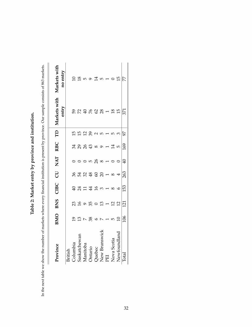
Tabl
e2:
Mar
kete
ntry
bypr
ovin
cean
din
stit
utio
n.
Inth
ene
xtta
ble
we
show
the
num
ber
ofm
arke
tsw
here
ever
yfin
anci
alin
stit
utio
nis
pres
entb
ypr
ovin
ce.O
ursa
mpl
eco
nsis
tsof
863
mar
kets
.
Prov
ince
BM
OB
NS
CIB
CC
UN
AT
RB
CT
DM
arke
tsw
ith
Mar
kets
wit
hen
try
noen
try
Brit
ish
Col
umbi
a19
2340
360
3415
5910
Sask
atch
ewan
1316
2454
029
1572
18M
anit
oba
79
1132
026
1240
5O
ntar
io38
3544
485
4339
769
Que
bec
60
1660
268
262
14N
ewBr
unsw
ick
713
320
89
528
5PE
I1
11
11
11
11
Nov
aSc
otia
512
88
014
518
0N
ewfo
undl
and
1012
64
05
315
15To
tal
106
121
153
263
4016
997
371
77
32

Table 3: Summary statistics for markets considered in estimation by type of entrant.
Summary statistics of markets considered in estimation, for markets where only Big6 or CU enter. A t-test for signifi-cant differences in the means of the variables appear in the last column. *, **, and *** indicate statistical significance atthe 0.10, 0.05, and 0.01 levels, respectivelySource: Stats Canada.
Big6 enter only CU enter only t-test: Big6 - CUVariable mean se mean se t
Population 5,803 728 1,502 253 5.58***Total income 23,773 486 21,116 696 3.13***Proportion French (in %) 4.62 1.01 32.27 5.23 -5.19***Number of business 475 56 143 17 5.72***Unemployment rate (in %) 10.53 0.70 14.00 1.15 -2.56**
33

Table 4: Summary statistics for demographic and product characteristics, and bank proximity.
Summary statistics for demographic characteristics of households, fees/rates, credit limits and product characteristicsand proximity of branches. Variables are defined in Appendix. Source: CFM database and bank branches database.
Variable mean sd min p1 p25 p50 p75 p99 N
Accounts: Fees (dollars) 6.85 15.32 0.00 0.00 0.00 0.00 8.00 81.00 6,135Accounts: Balance (in 10,000 dollars) 0.49 1.52 0.00 0.00 0.03 0.15 0.45 5.50 6,135Accounts: Checking account 0.61 0.49 0.00 0.00 0.00 1.00 1.00 1.00 6,135Accounts: Length relationship 5.81 1.67 1.00 1.00 5.00 7.00 7.00 7.00 6,135
Cards: Fees (dollars) 17.69 39.86 0.00 0.00 0.00 0.00 15.00 160.00 5,581Cards: Limits (1000s dollars) 9.08 8.56 0.00 0.00 3.00 7.00 13.00 36.00 5,581Cards: Credit protection 0.25 0.43 0.00 0.00 0.00 0.00 0.00 1.00 5,581Cards: Rewards 0.26 0.44 0.00 0.00 0.00 0.00 1.00 1.00 5,581
LOC: Rates (in %) 5.12 3.34 0.00 0.00 3.25 5.34 7.00 14.80 2,162LOC: Limits (1000s dollars) 35.26 47.65 0.00 0.30 12.50 22.50 45.00 212.50 2,162LOC: Fixed rate 0.33 0.47 0.00 0.00 0.00 0.00 1.00 1.00 2,162LOC: Secured line of credit 0.55 0.50 0.00 0.00 0.00 1.00 1.00 1.00 2,162LOC: Length relationship 6.05 1.41 1.00 2.00 5.00 7.00 7.00 7.00 2,162
Demographic variables:Assets (in 100,000s) 0.86 2.10 0.00 0.00 0.02 0.10 0.71 10.25 5,893Age 55.21 15.25 18.00 22.00 45.00 56.00 66.00 86.00 5,893Size household 2.24 1.13 1.00 1.00 2.00 2.00 3.00 6.00 5,893Own house 0.82 0.39 0.00 0.00 1.00 1.00 1.00 1.00 5,893Difficulty paying debt 2.96 2.52 0.00 0.00 1.00 2.00 5.00 9.00 5,893Employed 0.90 0.29 0.00 0.00 1.00 1.00 1.00 1.00 5,893Uses financial advisor 0.35 0.48 0.00 0.00 0.00 0.00 1.00 1.00 5,893University degree 0.83 0.37 0.00 0.00 1.00 1.00 1.00 1.00 5,893Married 0.76 0.43 0.00 0.00 1.00 1.00 1.00 1.00 5,893Income (in 100,000) 0.62 0.50 0.08 0.08 0.28 0.50 0.80 2.50 5,893Sophisticated investor 0.38 0.49 0.00 0.00 0.00 0.00 1.00 1.00 5,893
Proximity of branches:Number FIs in circle radious 10km 4.06 1.93 0.00 0.00 2.00 5.00 6.00 7.00 5,893FI for ACC is in circle radious 10km 0.84 0.37 0.00 0.00 1.00 1.00 1.00 1.00 6,135FI for CARD is in circle radious 10km 0.80 0.40 0.00 0.00 1.00 1.00 1.00 1.00 5,581FI for LOC is in circle radious 10km 0.84 0.37 0.00 0.00 1.00 1.00 1.00 1.00 2,162
34

Table 5: Estimates of entry model (I).
We show estimates of the elements of the profit function (Eq. 2) in the the entry model. Demographic variables havebeen normalized by their mean. "Competitive effect of X on Y" is the effect on the profit of financial institution Y iffinancial institution X enters in the market. Standard errors in parentheses obtained using bootstrap.
Variable Entry model
Panel A: Competitive effects:Competitive effect of BIG6 on BIG6 0.04499
(0.02179)Competitive effect of CU on BIG6 0.24508
(0.03198)Competitive effect of BIG6 on CU -0.06866
(0.02342)
Panel B: Demographic variables:Intercept -0.96986
(0.08476)Population BIG6 -0.00096
(0.02264)Population CU 0.20220
(0.02113)Income BIG6 0.00680
(0.02097)Income CU 0.17917
(0.02430)Unemployment BIG6 -0.26600
(0.03510)Unemployment CU -0.29688
(0.02927)Business activity BIG6 0.19471
(0.02312)Business activity CU -0.11042
(0.01934)Proportion French BIG6 -0.16209
(0.02738)Proportion French CU 0.19254
(0.02401)
35

Table 6: Estimates of entry model (II).
We show estimates of the elements of the profit function (Eq. 2) in the the entry model. Size and distance to headquarterare normalized by their mean. Standard errors in parentheses obtained using bootstrap.
Variable Entry model
Panel C: Provincial effects:British Columbia 0.18568
(0.02193)Manitoba 0.26834
(0.02705)New Brunswick 0.46453
(0.04539)Newfoundland and Labrador 0.45780
(0.04642)Nova Scotia 0.51770
(0.05128)Prince Edward Island 0.45050
(0.04790)Quebec 0.16603
(0.02357)Saskatchewan 0.14108
(0.01756)
Panel B: Firm-level effects:National Size 0.44322
(0.04583)Regional Size 0.05438
(0.02134)BMO 0.14693
(0.02125)BNS -0.06172
(0.01642)CIBC 0.28283
(0.03228)CU 0.52861
(0.05185)NBC -0.99947
(0.10124)distance to historical HQ -0.26752
(0.03353)distance to historical HQ (square) -0.01513
(0.01987)
36

Table 7: Entry barriers by financial institution and province
We estimate the level of entry barriers by financial institution and province. They are calculated by addying theconstant term, the bank fixed effects, and the provincial fixed effects from Table 6.
Province BMO BNS CIB CU NAT RBC TDBritish Columbia -0.6 -0.8 -0.5 -0.3 -1.8 -0.8 -0.8Manitoba -0.6 -0.8 -0.4 -0.2 -1.7 -0.7 -0.7New Brunswick -0.4 -0.6 -0.2 0.0 -1.5 -0.5 -0.5NFL-Labrador -0.4 -0.6 -0.2 0.0 -1.5 -0.5 -0.5Nova Scotia -0.3 -0.5 -0.2 0.1 -1.5 -0.5 -0.5Ontario -0.8 -1.0 -0.7 -0.4 -2.0 -1.0 -1.0PEI -0.4 -0.6 -0.2 0.0 -1.5 -0.5 -0.5Quebec -0.7 -0.9 -0.5 -0.3 -1.8 -0.8 -0.8Saskatchewan -0.7 -0.9 -0.5 -0.3 -1.8 -0.8 -0.8
37

Table 8: Estimates for adoption of financial products.
We show estimates of the adoption equation for the three financial products considered. We also show probit estimates.Household variables, and provincial and year fixed effects used in all cases. Standard errors in parentheses obtainedusing bootstrap (for structural model).
Accounts Credit cards Lines of creditVariable Structural Probit Structural Probit Structural Probit
Financial advisor 0.05698 0.03409 0.07558 0.04260(0.00751) (0.01781) (0.01111) (0.02352)
Heavy usage 0.08473 0.04575 0.07960 0.02176(0.01438) (0.00414) (0.01884) (0.00425)
Sophisticated 0.04943 0.02608 0.10536 0.07235(0.00826) (0.01929) (0.01455) (0.02611)
Close provider 0.82572 0.80525 0.66973 0.63894 0.68709 0.64906(0.07048) (0.01831) (0.07368) (0.01795) (0.06635) (0.02593)
Household variables YES YES YES YES YES YESProvincial fixed effects YES YES YES YES YES YESYear fixed effects YES YES YES YES YES YESNumber ofhousehold-year-bank product 41251 41251 41251 41251 41251 41251
38

Table 9: Estimates for fees/rates equations.
We show estimates of the fees/rates equations for the three financial products considered. We compare structuralestimates, and estimates from OLS. Account/card fees and lines of credit rates are expressed in logs. Account balanceexpressed in 10,000 dollars. Length relationship is a categorical variable with values 1-7 (see Appendix for definitions).LOC annual interest rates are expressed in logs. Credit limit expressed in logs. Household variables, bank, provincialand year fixed effects used in all cases. Standard errors in parentheses obtained using bootstrap (for structural model).
Accounts Credit cards Lines of creditVariable Structural OLS Structural OLS Structural OLS
Account balance -0.03601 -0.03610(0.00387) (0.02468)
Checking account 0.16995 0.16979(0.01771) (0.05353)
Card protection 0.34655 0.34683(0.03744) (0.08595
Rewards 1.95571 1.95581(0.19593) (0.10687
Limit (in logs) 0.19425 0.19708 0.16601 0.16556(0.01862) (0.01700) (0.01644) (0.05803)
Fixed rate 0.13933 0.13914(0.01413) (0.11107)
Secured 0.18260 0.18224(0.01772) (0.11343)
Length relationship 0.05990 0.05966 0.00198 -0.00240(0.00745) (0.01751) (0.00288) (0.03849)
Close provider -0.37887 0.13316 -0.41602 0.15251 -0.26144 -0.25080(0.03279) (0.08256) (0.04182) (0.10951) (0.02503) (0.16550)
Number of competitors -0.07236 -0.04943 -0.16207 -0.01766 0.05554 0.06022(0.00852) (0.01620) (0.01608) (0.02398) (0.00703) (0.03313)
Household variables YES YES YES YES YES YESBank fixed effects YES YES YES YES YES YESProvincial fixed effects YES YES YES YES YES YESYear fixed effects YES YES YES YES YES YESNumber ofhousehold-year-bank product 6135 6135 5581 5581 2162 2162
39
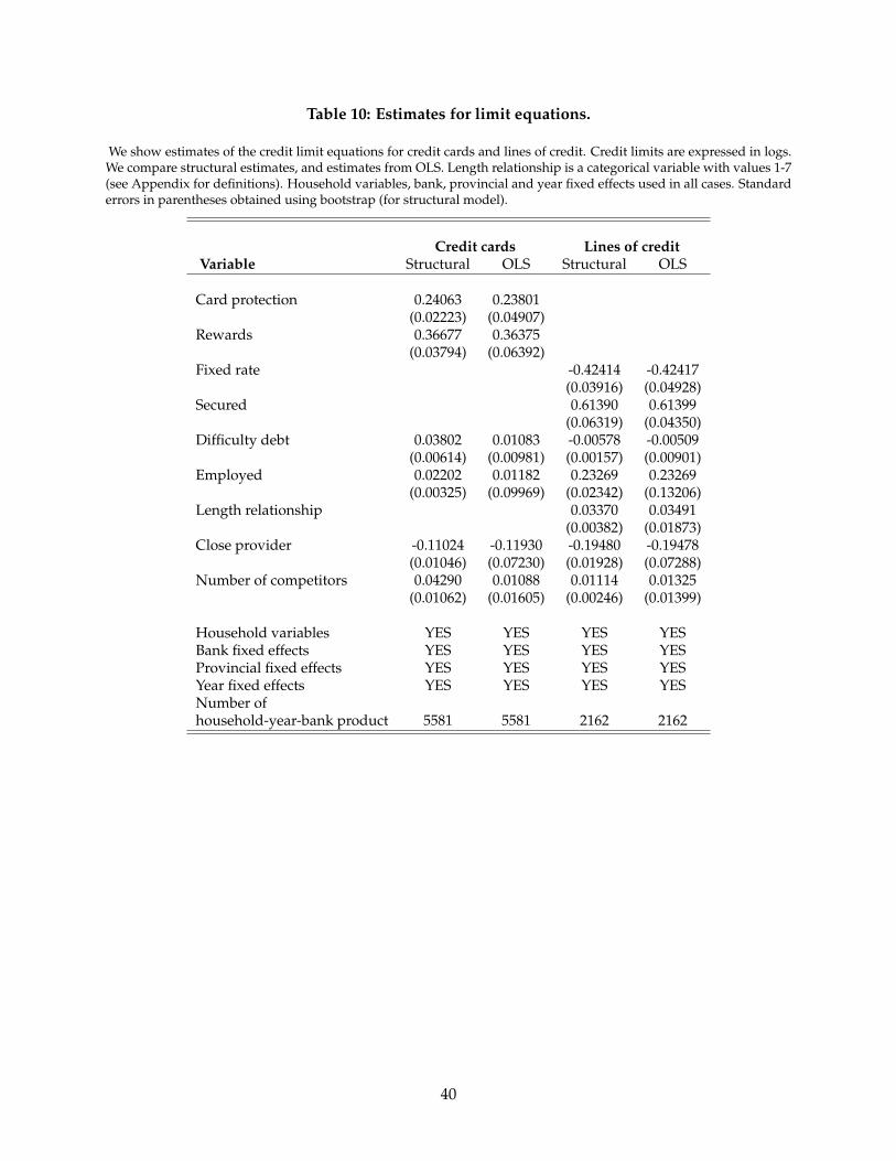
Table 10: Estimates for limit equations.
We show estimates of the credit limit equations for credit cards and lines of credit. Credit limits are expressed in logs.We compare structural estimates, and estimates from OLS. Length relationship is a categorical variable with values 1-7(see Appendix for definitions). Household variables, bank, provincial and year fixed effects used in all cases. Standarderrors in parentheses obtained using bootstrap (for structural model).
Credit cards Lines of creditVariable Structural OLS Structural OLS
Card protection 0.24063 0.23801(0.02223) (0.04907)
Rewards 0.36677 0.36375(0.03794) (0.06392)
Fixed rate -0.42414 -0.42417(0.03916) (0.04928)
Secured 0.61390 0.61399(0.06319) (0.04350)
Difficulty debt 0.03802 0.01083 -0.00578 -0.00509(0.00614) (0.00981) (0.00157) (0.00901)
Employed 0.02202 0.01182 0.23269 0.23269(0.00325) (0.09969) (0.02342) (0.13206)
Length relationship 0.03370 0.03491(0.00382) (0.01873)
Close provider -0.11024 -0.11930 -0.19480 -0.19478(0.01046) (0.07230) (0.01928) (0.07288)
Number of competitors 0.04290 0.01088 0.01114 0.01325(0.01062) (0.01605) (0.00246) (0.01399)
Household variables YES YES YES YESBank fixed effects YES YES YES YESProvincial fixed effects YES YES YES YESYear fixed effects YES YES YES YESNumber ofhousehold-year-bank product 5581 5581 2162 2162
40

Table 11: Estimates of elements of the covariance matrix.
We show estimates of the elements of the variance-covariance matrix used in our econometric model. Standard errorshave been generated using bootstrap.
Variable Accounts Credit cards Lines of credit
σF or σR 2.00197 2.56953 2.38778(0.20246) (0.25707) (0.25082)
σL 1.78253 -0.08745(0.17706) (0.00882)
ρπ,D -0.17674 -0.78654 0.06195(0.01916) (0.08470) (0.01242)
ρπ,F or ρπ,R 0.00043 0.57543 -1.25431(0.01260) (0.05366) (0.12708)
ρπ,L -0.68954 0.37487(0.07702) (0.03904)
ρD,F or ρD,R 0.46186 0.77267 -0.00097(0.04822) (0.07717) (0.00441)
ρD,L -1.20804 -0.08745(0.13194) (0.00882)
41
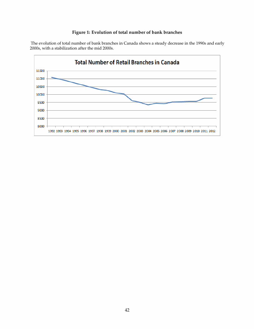
Figure 1: Evolution of total number of bank branches
The evolution of total number of bank branches in Canada shows a steady decrease in the 1990s and early2000s, with a stabilization after the mid 2000s.
42

Figure 2: Entry and population
This figure of number of entrants vs. population shows a clear positive correlation between the two. Wealso see that most markets have 6 entrants or less.
43

Figure 3: Example of market: Moose Jaw in Saskatchewan (I)
44

Figure 4: Example of market: Moose Jaw in Saskatchewan (II)
This map highlights the various bank branches in Moose Jaw (Saskatchewan). Each dot represents abranch, and different colors represent different institutions.
45

Figure 5: Markets considered and CFM households
This diagram shows the selection of markets and CFM households included in our estimation.
46