the price of one sweet calorie - agecon...

International Journal of Food and Agricultural Economics

ISSN 2147-8988, E-ISSN: 2149-3766

Vol. 3 No. 4, 2015, pp. 1-14

1

THE PRICE OF ONE SWEET CALORIE

Sebastien Buttet

Business Administration Division, Guttman CC, City University of New York, USA

Veronika Dolar Economics Department, Long Island University, Brookville, NY 11548, USA

E-mail: [email protected]

Abstract

We propose a new measure for food prices to further examine the impact of changes in

food prices and real income on individuals’ eating decisions and weight. We calculate price

per calorie for food consumed away from home and food consumed at home as the dollar

amount spent by households on each food category divided by the number of calories

consumed. We use our newly constructed time series for price per calorie as an input into a

neoclassical model of eating decisions and weight. Our goal is to propose a quantitative

explanation for the increase in calories consumed away from home as well as changes in

weight for men and women 1971 and 2006. We find that prices determine the allocation of

calories across food types, while income determines the total number of calories consumed

and thus individuals' weight. Based on our results, we share the view that taxes on food will

impact what people eat but will have limited effect on reducing the population body-mass

index or the obesity prevalence.

Keywords: Obesity, body weight, food prices, household income

1. Introduction

Two decades of intense research in the field of economics of obesity have improved our

understanding of the impact of food prices on weight and food choices and two critical

results have gained wide acceptance. First, several empirical studies show that changes in

aggregate food prices over time have little effect on the population body mass index or

obesity prevalence (e.g., Chou, Grossman, & Saffer, 2004; Beydoun, Powell, & Wang, 2008;

Anderson & Matsa, 2011). Second, experimental studies show that changes in the price of

selected food items drastically affects what people eat. For example, French et al. (2001) find

that a fifty percent price reduction on low-fat snacks in vending machines at schools and

work places increase the percentage of low-fat snack sales by ninety three percent. These two

results about the effect of food prices on weight and food choices are important because of

their influence on the public health debate about the effectiveness of fiscal policies for

winning the fight against the obesity epidemic. A common view held by policymakers is that

taxes applied selectively to different food items work effectively to reduce consumption of a

particular type of food or ingredient (e.g., ban of trans-fats) but are unlikely to produce

significant changes in body-mass index or obesity prevalence (Powell, Chriqui, &

Chaloupka, 2009; Chouinard, Davis, LaFrance, & Perloff, 2012).

In this paper, we further examine the impact of changes over time in food prices and

household real income on individuals' food choices and weight using a calibrated static

model. Our first objective is to propose a new measure for food prices to further examine the

The Price of One Sweet Calorie

2

impact of changes in food prices and real income on individuals’ eating decisions and

weight. We calculate price per calorie for food consumed away from home and food

consumed at home as the dollar amount spent by households on each food category divided

by the number of calories consumed. Our second objective is to contribute to the debate

about the impact of food prices and household real income on weight and food choices using

a different modeling strategy. We ask how much of the increase in calories consumed away

from home as well as changes in weight for men and women between 1971 and 2006 can be

accounted for by changes in food prices and household real income. Our final, and perhaps

the most critical objective, is to use economic theory and available evidence from medical

research on obesity to look inside the black box of how people make eating decisions and to

improve our understanding of what determines the (low) food price elasticity of weight.

In this paper we assume that there is a one-to-one relationship between agent's weight

and total calories consumed. In addition, weight affects the probability that agents are alive.

Given household real disposable income and the relative price of a calorie (at home versus

away from home), agents decide how much to eat at each location as well as how much of

the non-food good to consume to maximize their expected utility.

Identification of the model is clean. On the one hand, we use available evidence from

medical research on nutrition to calibrate the parameters of the weight function and medical

research on obesity-related diseases to fit the survival probability function. On the other

hand, we choose the remaining preferences parameters to match the mean weight and

fraction of calories away from home observed in NHANES 19711, allowing some preference

heterogeneity between men and women.

We use the calibrated model to assess the impact of changes in food prices and household

real income on food choices and weight between 1971 and 2006. We find that prices

determine the allocation of calories across food types, while income determines the total

number of calories consumed and thus individuals' weight. Based on our results, we share the

view that taxes on food will impact what people eat but will have limited effect on reducing

the population body-mass index or the obesity prevalence.

The remainder of the paper is organized as follows. In Section 2, we describe data about

weight and calories consumed at and away from home. In Section 3, we introduce our new

method of calculating per calorie food prices and show the household real income between

1971 and 2006. In Section 4 and Section 5, we develop and calibrate our model and we

conduct our simulations in Section 6. Finally, we offer concluding remarks in Section 7.

2. Nutrition Data

In this section, we use two distinct data sets from the National Health and Nutritional

Examination Survey (NHANES) to document changes over time in Body-Mass Index (BMI),

weight, and the fraction of calories consumed away from home for men and women for the

period between 1971 and 2006 (see Table 1).2 Data about weight comes from the

1 The data for NHANES I was collected during the period 1971-75 however, for clarity and

convenience we will refer to it as NHANES 1971 and refer to it by year 1971. Similar, the

data for NHANES 2005-2006 was collected over these two years, however, we will refer to

it as NHANES 2006 and refer to it by year 2006 throughout the paper. 2 Body-mass index is a measure of body fat based on height and weight that equally applies

to adult men and women. It is calculated as 703 times weight measured in pounds divided by

height squared measured in inches squared. Individuals with BMI lower than 18.5 are

considered underweight, between 18.5 and 24.9 normal weight, between 25 and 30

overweight, and 30 or greater obese. BMI combined with other information about waist

S. Buttet and V. Dolar

3

examination component of NHANES and is measured by trained medical personnel. The

fraction of calories consumed away from home, on the other hand, is self-reported by

individuals.3

Table 1. Changes in BMI, Weight, Calories, and Fraction of Calories Consumed Away

From Home for Men and Women

1971 2006 % Change

Men

BMI 25.9 29.0 12.0

Weight (lbs) 175.7 198.2 12.8

Calories 2433 2543 4.5

% calories away 29.9 40.5 35.5

Women

BMI 25.2 28.8 14.3

Weight (lbs) 145.8 168.9 15.8

Calories 1538 1802 17.2

% calories away 19.5 35.9 84.1

In the last thirty years, men have gained on average 23 pounds and their body-mass index

increased from 25.9 (slightly overweight) to 29.0 (borderline obese).4 The increase in

average weight and body-mass index is even more pronounced in percentage terms for

women who also gained 23 pounds. In addition, men and women changed their eating habits

dramatically and ate out more. Total daily calories consumed increased by 110 calories for

men and 264 for women, while the fraction of calories away from home increased by 35.5

and 84.1 percentage points for men and women, respectively.

3. Price per Calorie

As already mentioned, in the field of public health numerous controlled experimental

studies have been developed that show that changes in the price of selected food items

drastically affects what people eat (e.g., Jeffery, French, Raether, & Baxter, 1994; French,

2003; Epstein, Dearing, Paluch, Roemmich, & Cho, 2007). Because the above studies imply

great price sensitivity they have clear implications for public health policy. For example,

lowering prices on healthy foods and hiking the prices of unhealthy foods can induce people

circumference and other factors such as physical activity, cigarette smoking, or low-density

cholesterol level gives a risk assessment of developing obese-associated diseases such as

heart attacks, diabetes II, strokes, etc. 3 The question about where do people eat their meal has changed over time. In NHANES

1971, individuals can choose among the following four locations: at home, in school, in

restaurants, and other, while in NHANES 2006, the location question is: “Did you eat this

food at home?” and the possible answers are yes, no, refused to answer, do not know, and

missing information. We get rid of a small fraction of missing values or unknowns. To

maintain consistency across the two data sets, we define food eaten at home as any food item

for which individuals answered “at home” in NHANES 1971 and “yes” in NHANES 2006.

We define food eaten away from home as all food items not eaten at home. We then

calculate the fraction of calories eaten away from home as one minus the fraction of calories

eaten at home. 4 Simple t-tests show that differences in mean weight and mean body-mass index over time

are statistically significant for both men and women.


4

to buy more of the former and less of the latter (Brownell & Frieden, 2009; Brownell et al.,

2009).

Price sensitivity of demand, however, is only a necessary and obviously not a sufficient

condition to reduce food consumption and body weight. For example, take two food items

with the same price elasticity of demand but where one is more calorie-dense than the other.

Then the same tax will equality decrease quantity demanded (measured in pounds of food for

example) of these two food items but will have drastically different impact on body weight;

the decrease in the quantity demanded of high caloric food will have a much bigger effect on

body weight. This issue can be ameliorated by studying the impact of changes in price per

calorie (“Calorie” will be used in lieu of kilocalorie throughout the paper) instead of looking

at regular food item prices, since the change in quantity demanded measured in calories more

directly translates in changes in body weight.

In addition, a problem with experimental studies is that they only include a very limited

amount of items and focus on the consumption changes only at one point in time (e.g. at

lunch or at school). As a result, one cannot observe how a person behaves outside the

parameters of the experiment. For example, if individuals substitute away from highly priced

or taxed foods at the vending machine towards other lower-priced but potentially highly

caloric foods there will be no significant change in body weight (in fact, weight might

actually increase). A soda tax might induce people to switch to other high-caloric drinks such

as orange juice or chocolate milk at home, with no impact on their weight. In this case

including only few food items ignores the possibility for substitution. This can be somewhat

improved by including all possible food items, which is impossible or by allowing for more

broadly defined food groups such as food at home and food away from home.

Economists have been trying to add to this line of work by using larger observational data

to analyze the relationship between food prices and weight but with mixed success. For

example, several empirical studies show that changes in aggregate food prices over time

have little effect on the population body-mass index (BMI) or obesity prevalence for adults

(Beydoun et al., 2008; Goldman, Lakdawalla, & Zheng, 2011) and almost no effect on

children and adolescents (Sturm, Powell, Chriqui, & Chaloupka, 2010, Powell & Chaloupka,

2011). As concluded by Lakdawalla and Zheng (2011) the current literature on how food

prices affect body weight suffers from substantial empirical challenges of causal inference

that have not yet been satisfactory overcome.

One such challenge comes from the measurement of food prices themselves. In order to

identify the effect of food prices on body weight researches have use two familiar data

sources: Bureau of Labor Statistics (BLS) and Council of Community and Economic

Research (C2ER), formerly known as American Chamber of Commerce Researchers

Association (ACCRA). The common problem with using these data sets is that they use only

around 20 to 60 food items. Given the fact that about 320,000 foods and beverage products

are available it the United States, and that an average supermarket carries 30,000 to 40,000

of them, this seems very limited (Nestle, 2006).

In this section, we introduce a new method to measure much broader average prices that

adjusts for changes in calories consumed over time. Using household expenditures share data

for different food categories we calculate the price per calorie as household expenditures on

food divided by calories consumed. The logic behind construction of price per calorie in this

paper is quite simple. Divide the amount of money spent on a certain food item by the

number of calories consumed for this food. A similar strategy is used elsewhere where they

take the price per unit of food item and divide it by the calories per unit of food (Grossman,

Tekin, & Wada, 2013; Goldman et al., 2011;Christian and Rashad 2009). The difference

with our approach is that instead of focusing on a specific food item, we can take broad food

categories and calculate price per calorie for that category.


5

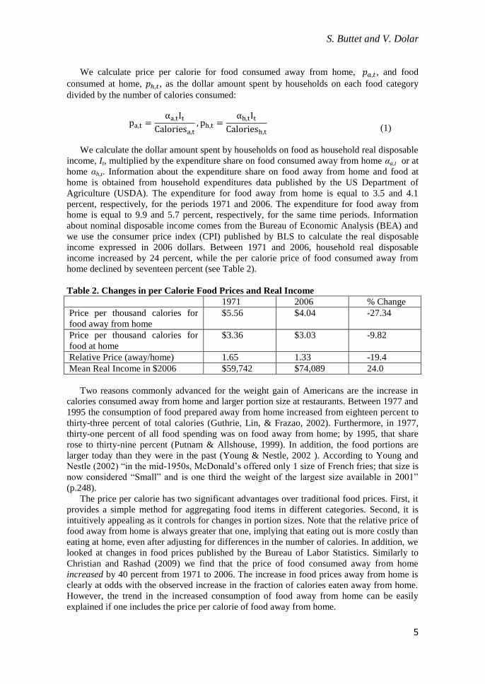
We calculate price per calorie for food consumed away from home, 𝑝𝑎,𝑡, and food

consumed at home, 𝑝ℎ,𝑡, as the dollar amount spent by households on each food category

divided by the number of calories consumed:

pa,t =αa,tIt

Caloriesa,t

, ph,t =αh,tIt

Caloriesh,t

(1)

We calculate the dollar amount spent by households on food as household real disposable

income, It, multiplied by the expenditure share on food consumed away from home αa,t or at

home αh,t. Information about the expenditure share on food away from home and food at

home is obtained from household expenditures data published by the US Department of

Agriculture (USDA). The expenditure for food away from home is equal to 3.5 and 4.1

percent, respectively, for the periods 1971 and 2006. The expenditure for food away from

home is equal to 9.9 and 5.7 percent, respectively, for the same time periods. Information

about nominal disposable income comes from the Bureau of Economic Analysis (BEA) and

we use the consumer price index (CPI) published by BLS to calculate the real disposable

income expressed in 2006 dollars. Between 1971 and 2006, household real disposable

income increased by 24 percent, while the per calorie price of food consumed away from

home declined by seventeen percent (see Table 2).

Table 2. Changes in per Calorie Food Prices and Real Income

1971 2006 % Change

Price per thousand calories for

food away from home

$5.56 $4.04 -27.34

Price per thousand calories for

food at home

$3.36 $3.03 -9.82

Relative Price (away/home) 1.65 1.33 -19.4

Mean Real Income in $2006 $59,742 $74,089 24.0

Two reasons commonly advanced for the weight gain of Americans are the increase in

calories consumed away from home and larger portion size at restaurants. Between 1977 and

1995 the consumption of food prepared away from home increased from eighteen percent to

thirty-three percent of total calories (Guthrie, Lin, & Frazao, 2002). Furthermore, in 1977,

thirty-one percent of all food spending was on food away from home; by 1995, that share

rose to thirty-nine percent (Putnam & Allshouse, 1999). In addition, the food portions are

larger today than they were in the past (Young & Nestle, 2002 ). According to Young and

Nestle (2002) “in the mid-1950s, McDonald’s offered only 1 size of French fries; that size is

now considered “Small” and is one third the weight of the largest size available in 2001”

(p.248).

The price per calorie has two significant advantages over traditional food prices. First, it

provides a simple method for aggregating food items in different categories. Second, it is

intuitively appealing as it controls for changes in portion sizes. Note that the relative price of

food away from home is always greater that one, implying that eating out is more costly than

eating at home, even after adjusting for differences in the number of calories. In addition, we

looked at changes in food prices published by the Bureau of Labor Statistics. Similarly to

Christian and Rashad (2009) we find that the price of food consumed away from home

increased by 40 percent from 1971 to 2006. The increase in food prices away from home is

clearly at odds with the observed increase in the fraction of calories eaten away from home.

However, the trend in the increased consumption of food away from home can be easily

explained if one includes the price per calorie of food away from home.


6

4. A Simple Optimization Model Of Eating Decision And Weight

We propose a static model where agents decide how much and where to eat (out or at

home) as well as non-food consumption. We let a and h be the number of calories consumed

away and at home, respectively, and cnf

represents non-food consumption. Calories away and

at home are aggregated using a constant elasticity of substitution (CES) function to obtain

food consumption:

𝑐𝑓 = (𝜂𝑎𝜌 + (1 − 𝜂)ℎ𝜌)1

𝜌 (2)

(2)

with 𝜂 ∈ (0,1) and 𝜌 ∈ (−∞, 1]. Food away and at home are perfect substitutes, Cobb-

Douglas, or perfect complements when the parameter ρ is equal to one, zero, or minus

infinity, respectively. The parameter η reflects consumer's preference for eating at home or

eating out.

Preferences of the representative agent are Cobb-Douglas and are given by:

𝑈(𝑐𝑓 , 𝑐𝑛𝑓) = (𝑐𝑓)𝛼(𝑐𝑛𝑓)1−𝛼 (3)

(3)

with 𝛼 ∈ (0,1).

Agents make ex-ante eating decisions understanding that weight affects the probability

π(W) of being alive. We assume that the function π is an inverted U-shape function of BMI

which implies that agents who are either over- or underweight have a greater chance to die.

Finally, agents receive utility U ≤ 0 when they die. The expected utility is equal to:

𝜋(𝑊)𝑈(𝑐𝑓 , 𝑐𝑛𝑓) + (1 − 𝜋(𝑊))𝑈 (4)

(4)

Note that it is never optimal for people to eat so much that they would die with certainty

since 𝑈(𝑐𝑓 , 𝑐𝑛𝑓) is positive and 𝑈 ≤ 0.

The relationship between weight and calorie consumption is given by the simple linear relationship:

𝑊 = 𝜇 + 𝜃(𝑎 + ℎ)5 (5)

(5)

with θ > 0.

Finally, the budget constraint of the representative agent is given by:

𝑐𝑛𝑓 + 𝑝ℎℎ + 𝑝𝑎𝑎 = 𝐼 (6)

(6)

5 Body weigh quite obviously depends on physical exercise as well. Equation (5) in principle

does not exclude weight being dependent on other factors. All other factors that determine

weight such as height, gender, and physical effort are potentially captured with parameter 𝜇.

The assumption that we are making is that all these other factors are constant for all

individuals and vary only by gender. Since we are looking at an average American man and

woman in the US we assume that his/her height remained unchanged between 1971 – 2006, a

fact supported by the data. In addition, we also keep the level of exercise, physical effort, and

energy expenditure constant. This assumption is based on the paper by Cutler, Glaeser, &

Shapiro (2003)In this paper they examine two components of energy expenditure: voluntary

exercise, and involuntary energy expenditure associated with employment and conclude that

their results suggest that increased caloric intake explains the rise in obesity, not reduced

caloric expenditure.


7

where we normalized the price of non-food to one, ph and pa are the real price of food at

and away from home, respectively, and agents are endowed with real income I.

For any prices and income, {ph, pa, I}, the representative agent chooses optimal calories

from food away and at home as well as non-food consumption, {a, h, cnf

}, to maximize the

expected utility in equation (4) subject to the budget constraint (6), the weight function (5),

the food aggregation equation (2), and non-negativity constraints for calorie and non-food

consumption.

We substitute the weight relationship into the objective function in equation (4). The

consumption of food away from home, a, and food at home, h, appear as follows in the

objective function:

𝜋(𝜇 + 𝜃(𝑎 + ℎ))(𝜂𝑎𝜌 + (1 − 𝜂)ℎ𝜌)𝛼𝜌(𝐼 − 𝑝ℎℎ − 𝑝𝑎𝑎)1−𝛼

+ (1 − 𝜋(𝜇 + 𝜃(𝑎 + ℎ)) ) 𝑈 (7)

We take first-order conditions with respect to food away from home, a, and food at home,

h.

[a]: 𝜃𝜋′(𝑊)(𝑈(𝑐𝑓 , 𝑐𝑛𝑓) − 𝑈) + 𝜋(𝑊)𝑈(𝑐𝑓 , 𝑐𝑛𝑓) (𝛼𝜂𝑎𝜌−1

𝜂𝑎𝜌+(1−𝜂)ℎ𝜌 −𝑝𝑎(1−𝛼)

𝐼−𝑝𝑎𝑎−𝑝ℎℎ) = 0

[h]: 𝜃𝜋′(𝑊)(𝑈(𝑐𝑓 , 𝑐𝑛𝑓) − 𝑈) + 𝜋(𝑊)𝑈(𝑐𝑓 , 𝑐𝑛𝑓) (𝛼(1−𝜂)ℎ𝜌−1

𝜂𝑎𝜌+(1−𝜂)ℎ𝜌 −𝑝ℎ(1−𝛼)

𝐼−𝑝𝑎𝑎−𝑝ℎℎ) = 0 (8)

(8)

Note that consumer’s utility might not be strictly concave because the survival

probability depends on consumer’s weight. As a result, it is not clear whether first-order

conditions are sufficient for optimality. Although we do not offer a formal proof, we check in

our computer simulations that the allocations that satisfy the first-order conditions in

equation (8) are also utility-maximizing (locally).

We rearrange the first-order conditions in equation (8). The optimal level of food away

from home, a, and food at home, h, are obtained by solving the following system of

equations (9):

𝜂𝑎𝜌−1 − (1 − 𝜂)ℎ𝜌−1

𝜂𝑎𝜌 + (1 − 𝜂)ℎ𝜌=

1 − 𝛼

𝛼

𝑝𝑎 − 𝑝ℎ

𝐼 − 𝑝𝑎𝑎 − 𝑝ℎℎ (9)

𝛼𝜂𝑎𝜌−1

𝜂𝑎𝜌 + (1 − 𝜂)ℎ𝜌−

𝑝𝑎(1 − 𝛼)

𝐼 − 𝑝𝑎𝑎 − 𝑝ℎℎ= 𝜃

𝜋′(𝜇 + 𝜂(𝑎 + ℎ))

𝜋(𝜇 + 𝜂(𝑎 + ℎ))(1 −

𝑈

𝑈(𝑐𝑓 , 𝑐𝑛𝑓))

(9)

In the reminder of the paper, we explain our method to calibrate the three key parts of our

model: the weight function, the survival probability function, and the deep preference

parameters. We then use the calibrated model to conduct a lab experiment where we assess

the impact of food price and real income on weight and the fraction of calories away from

home.

5. Calibration

We use medical research on obesity to calibrate the weight law of motion and the

survival probability function. We then chose the remaining preference parameters to match


8

the average weight and calories away from home for men and women observed in the

NHANES 1971 sample.

5.1. Weight Function

The weight function in equation (5) contains two distinct important parameters. First, the

constant θ converts calorie intake into weight. According to the dietary guidelines from the

US Department of Agriculture, people gain ten pounds per year if they eat an extra one

hundred calories every day above and beyond the recommended daily calorie intake. As a

result, we fix 𝜃 =10

100×365= 2.7397 × 10−4.

Second, we use the average observed weight and calorie consumption by men and

women in NHANES 1971 to fix μm and μ

f. The weight and total calories data comes from

Table 1.

𝜇𝑚 = 𝑊𝑚,1971 − 𝜃𝑐𝑎𝑙𝑚,1971 = 175.7 − 2.7397 × 10−4 × 2433 × 365 = −67.6

𝜇 𝑓 = 𝑊𝑓,1971 − 𝜃𝑐𝑎𝑙𝑓,1971 = 145.8 − 2.7397 × 10−4 × 1538 × 365 = −8.0

(

10)

5.2. Survival Probability Function

We posit that the survival probability function π(Wt) is given by the following functional

form:

𝜋(𝑊𝑡) =1

1 + 𝜅(𝑊𝑡 − 𝑊∗)2 (10)

(11)

with κ > 0 and W* > 0 represents the agent's “best” weight where the survival probability

is maximized and equal to one. Note that the survival probability increases with the agent's

weight when Wt ≤ W* but decreases once the agent's weight is greater than W*.

First, we set the best weight W*,m

= 170 for men and W*,f

= 145 for women which

corresponds to a body-mass index of 25 for both sexes.

Second, the parameter κ is identified by the increased mortality risk due to obesity alone.

For two different weight W1 and W2, the increased mortality is equal to:

1 − 𝜋(𝑊1)

1 − 𝜋(𝑊2)=

(𝑊1 − 𝑊∗)2

(𝑊2 − 𝑊∗)2×

1 + 𝜅(𝑊2 − 𝑊∗)2

1 + 𝜅(𝑊1 − 𝑊∗)2 (11)

(12)

Allison, Fontaine, Manson, & Stevens (1999) report the hazard ratios of death based on

six large prospective cohort studies where subjects are placed into two distinct groups: the

control group is comprised of individuals whose BMI is between twenty-three and twenty-

five; the treated group consists of individuals with BMI higher than twenty-five.

The death likelihood increases by a factor of 1.08 for overweight individuals (when BMI

is between 25 and 28) and by a factor of 1.43 for obese people (when BMI is between 30 and

35). Choosing the middle point for each interval, a BMI of 26.5 corresponds to a weight of

181 pounds for a male of average height, while a BMI of 32.5 corresponds of a weight of

221 pounds. As a result, the parameter 𝜅𝑚 is obtained by solving the following equation:

121

2601×

1 + 2601𝜅𝑚

1 + 121𝜅𝑚=

1.08

1.43 (12)

(13)

It is equal to 𝜅𝑚 = 2.39 × 10−2


9

Similarly, choosing the middle point for each interval, a BMI of 26.5 corresponds to a

weight of 153 pounds for a female of average height, while a BMI of 32.5 corresponds of a

weight of 188 pounds. As a result, the parameter 𝜅𝑤 is obtained by solving the following

equation: 64

1849×

1 + 1849𝜅𝑤

1 + 64𝜅𝑤=

1.08

1.43 (13)

(14)

It is equal to 𝜅𝑤 = 4.6 × 10−2

5.3. Preferences

We are now left with calibrating four preferences parameters, (𝛼, 𝜂, 𝜌, �̅�). First, since the

utility function 𝑈(𝑐𝑓 , 𝑐𝑛𝑓) is positive, we fix 𝑈 = 0 so that death resulting from excess

eating is never an optimal choice.

Second, we use the research of Reed, Lavedahl, & Hallahan (2005) which estimates the

elasticity of substitution between food away from home and food consumed at home. They

find that both types of foods are substitutes and a result, we fix 𝜌 = 0.75.

Finally, we use the two first-order conditions in equation (9) to determine (𝛼, 𝜂) to match

the observed average weight and fraction of calories consumed away from home for men and

women in the NHANES 1971 sample.

Proposition 1 The calibrated parameter values of (𝛼, 𝜂) are given by:

𝜂 = 𝐵𝐺 + 𝐹𝐵 − 𝐺𝐸𝐷

𝐺(𝐴 + 𝐵) − 𝐴(𝐸 − 𝐹) + 𝐹𝐵 + 𝐺𝐸(𝐶 − 𝐷) (14)

𝛼 = 𝐸𝐺(𝐶𝜂 + 𝐷(1 − 𝜂))

(𝐸 − 𝐹)𝐴𝜂 + 𝐹𝐵(1 − 𝜂)

where 𝐴 = (𝑎1971)𝜌−1, 𝐵 = (ℎ1971)𝜌−1, 𝐶 = (𝑎1971)𝜌, 𝐷 = (ℎ1971)𝜌−1,

𝐸 =𝑝𝑎

1971 − 𝑝ℎ1971

𝐼 − 𝑝𝑎1971𝑎1971 − 𝑝ℎ

1971ℎ1971

,

𝐹 =𝑝𝑎

1971

𝐼 − 𝑝𝑎1971𝑎1971 − 𝑝ℎ

1971ℎ1971

,

𝐺 = −2𝜅𝜃(𝑊1971 − 𝑊∗)

1 + 𝜅(𝑊1971 − 𝑊∗)2

Proof: See the Appendix.

For the period 1971, men's average weight, total calories, and fraction of calorie

consumed away from home was equal 175.7 pounds, 2433 calories, and 29.9 percent,

respectively (see Table 1). This implies that calories at home and away from home are equal

to ℎ𝑚,1971 = 1705.5 and 𝑎𝑚,1971 = 727.5, respectively. Per calorie prices of food away

from home and food at home are equal to 𝑝𝑎1971 = 5.56 × 10−3 and 𝑝ℎ

1971 = 3.36 × 10−3.

Using the information about real income6 from Table 2, non-food daily consumption is equal

6 In principle, we would like to use separate income for men and women; however, the

NHANES data set we are using for information about weight and calories consumed has a

very limited information on income. Income appears in 4 broad categories, which is simply


10

to: 𝑐𝑛𝑓𝑚,1971= 𝐼1971 − 𝑝𝑎

1971𝑎𝑚,1971 − 𝑝ℎ1971ℎ𝑚,1971 = $153.9. Note that food expenditures

is equal to roughly five percent of income. By plugging all these numbers into equation (9)

we find that 𝜂𝑚 = 0.49 and 𝛼𝑚 = 0.15.

Similarly, we determine the coefficient 𝛼𝑤 and 𝜂𝑤 to match the observed average weight

and fraction of calories consumed away from home for women in the NHANES 1971

sample. For the period 1971, women's average weight, total calories, and fraction of calorie

consumed away from home was equal 145.8 pounds, 1538 calories, and 19.5 percent,

respectively (see Table 1). This implies that calories at home and away from home are equal

to ℎ𝑓,1971 = 1238.1 and 𝑎𝑓,1971 = 299.9, respectively. Using the information about food

prices and income from Table 2, non-food consumption is equal to 𝑐𝑛𝑓∗ = 157.8. By

plugging all these numbers into equation (7) we find that 𝜂𝑤 = 0.45 and 𝛼𝑤 = 0.12.

Note that men and women differ considerably in their preferences for food versus non-

food goods and food at home versus food away from home. The food share, 𝛼, and the

preference parameter for food away from home, 𝜂, are greater for men compared to women.

The heterogeneity across gender is not counter-intuitive since men tend to eat more than

women and they also eat more away from home. In the next section, we use the calibrated

model to assess the impact of changes in relative food prices and real income on eating

habits and weight of Americans between 1971 and 2006.

6. Simulations

We perform the following experiments. First, we change the price per calorie of food

away from home from its 1971 value, 𝑝𝑎1971 = 5.56 × 10−3, to its 2006 value, 𝑝𝑎

2006 =4.04 × 10−3 leaving all other parameters of the model constant. From the first-order

conditions in equation (7), we calculate the new values for food away from home and food at

home. We then calculate for men and women, respectively, as well as the resulting BMI. We

report results of the first experiment in the first column of Table 3. For men, the fraction of

calories away from home increases by 12 percentage points from 30 percent (calibrated value

from Table 1) to 42 percent. For women, the fraction of calories consumed away from home

increases by 8 percentage points from 19 percent (calibrated value) to 27 percent.7 The

impact on agent's weight is small. Men gain 1.5 pounds while and women gain only 0.2

pounds as their weight increases to 178 and 146 pounds, respectively.

The second experiment consists of changing the price per calorie of food at home from its

1971 value, 𝑝ℎ1971 = 3.36 × 10−3, to its 2006 value, 𝑝ℎ

2006 = 3.03 × 10−3 leaving all other

parameters constant. We calculate the new value for food away from home and food at home

as well as weight and body-mass index as explained above. We report the result in the

second column of Table 3. For men, the fraction of calories away from home decreases by 4

percentage points from 30 percent to 26 percent. For women, the fraction of calories away

from home decreases by 5 percentage points from 19 percent to 14 percent. Again, the

decline in food prices has little impact on agent's weight.

too limited to use for our exercise. As a result we use the same mean real income obtain from

the Bureau of Economic Analysis for both men and women. As a result, women and men

face the same, but looser budget constraint. 7 For men, results slightly overshoots the data as the observed fraction of calories consumed

away from home in 2006 is equal 41 percent. For women, results do not fully account for the

observed change in the data as the fraction of calories consumed away from home by women

in 2006 is equal to 36 percent.


11

Table 3. Average BMI, Weight, and Fraction of Calories Consumed Away Predicted by

the Model

Data

1971

Data

2006

pa ph Income All

Men

BMI 25.9 29.0 26 26 28 29

Weight (lbs) 175.7 198.2 178 175 194 197

Calories 2433 2543 2453 2425 2620 2644

% calories away 29.9 40.5 42 26 34 36

Women

BMI 25.2 28.8 25 25 29 30

Weight (lbs) 145.8 168.9 146 144 166 170

Calories 1538 1802 1539 1519 1738 1782

% calories away 19.5 35.9 27 14 21 24

The third experiment consists of changing household real disposable income from its

1971 value 𝐼1971 = $59,742 to its 2006 value 𝐼2006 = $74,089 (see Table 2) leaving all

other parameters constant. We report the results in the fifth column of Table 3. Changes in

income account for a large fraction of the observed change in individual's weight. The

weight of men and women increases to 194 and 166 pounds, respectively. Changes in

income also induce a reallocation effect. As agents become richer, the fraction of calories

consumed away from home increase from 30 percent to 36 percent for men and from 19

percent to 24 percent for women.

Finally, the fourth experiment consists of changing food prices and income all at once.

For men, the model predicts that a weight equal to 197 pounds and the fraction of calories

away from home is equal to 36 percent. For women, the model predicts that a weight equal to

170 pounds and the fraction of calories away from home is equal to 24 percent.

The lessons learned from the model for eating decisions and weight can be summarized

as follows. Changes in food prices have an “allocation” effect and have little impact on total

calories consumed and weight. As the price of one food category changes, households

substitute from one food category to another. Changes in income, on the other hand, have a

large impact on weight. Between 1971 and 2006, much of the increase in weight and BMI

can be accounted for by increase in household real disposable income.8

Our results corroborate the existing knowledge on obesity in the following way. On the

one hand, economists who use empirical models found that the impact of food prices on

weight is small (e.g., Chou, Grossman, & Saffer, 2004; Beydoun, Powell, & Wang, 2008;

Anderson & Matsa, 2011)). Using a fully specified calibrated dynamic model, we also find

that changes in food prices over time account for almost none of the weight gain by

Americans in the last thirty years. On the other hand, researchers in the field of public health

(e.g., French et al. 2001) design small-scale experiments to show that even small changes in

food prices can have strong local effect on individual's food choices. For example, the above-

mentioned authors examined the effect of lower prices on sales of lower fat vending machine

snacks in 12 work sites and 12 secondary schools. According to a study, price reductions of

8 Dolar (2009) shows that the positive relationship between body-mass index and household

income holds for men in several cross-sections of NHANES. For women, however, body-

mass index is negatively related to household income suggesting that some other force not

captured in our model is at work. We leave the task of reconciling the pattern differences for

body-mass index and household income in cross-section and time-series data for men and

women for future research.


12

ten percent, twenty five percent, and fifty percent on low-fat snacks in vending machines

increase the percentage of low-fat snack sales by nine, thirty nine, and ninety three percent,

respectively. Using our calibrated dynamic model, we also find that change in food prices

affect where people eat (at home or out).

7. Concluding Remarks

In this paper, we further analyzed the impact of changes in food prices and household

income on people’s eating decisions and weight using a static model with rational agents.

After careful calibration of the model using evidence from medical research on obesity, we

found that food prices determine the allocation of calories across food types, while

household income determine the total number of calories consumed and thus individual's

weight. Between 1971 and 2006, changes in food prices alone account for almost none of the

change in weight of Americans men and women. On the other hand, changes in household

income account for almost all of the increase in men's and women's weight. Because of the

limited effect of food price alone on the BMI, we support the view that taxes on food will

impact what people eat but will have limited effect on reducing the population BMI or the

obesity prevalence.

We see two important avenues for academic research on obesity as well as policy

recommendation. First, educating people about the benefits of eating healthy, exercising

regularly, and the negative health consequences of being obese seem to be promising policies

to win the fight against obesity epidemic. Economic research is needed to measure the

impact of these education programs on individual's weight and BMI.

Second, we derived our results for the impact of food prices on weight and food choices

in an environment where agents are fully rational. An alternative view point is that there is

nothing optimal in being obese and that individuals experience commitment problems when

making food decisions. It is an open and interesting question to revisit the impact of food

prices and household income in a set-up where agents have time-inconsistent preferences à la

Laibson (1997). We leave these two tasks for future research.

8. Appendix – Proof Of Proposition 1

Proposition 1 The calibrated parameter values of (𝛼, 𝜂) are given by:

𝜂 = 𝐵𝐺 + 𝐹𝐵 − 𝐺𝐸𝐷

𝐺(𝐴 + 𝐵) − 𝐴(𝐸 − 𝐹) + 𝐹𝐵 + 𝐺𝐸(𝐶 − 𝐷)

𝛼 = 𝐸𝐺(𝐶𝜂 + 𝐷(1 − 𝜂))

(𝐸 − 𝐹)𝐴𝜂 + 𝐹𝐵(1 − 𝜂)

where 𝐴 = (𝑎1971)𝜌−1, 𝐵 = (ℎ1971)𝜌−1, 𝐶 = (𝑎1971)𝜌, 𝐷 = (ℎ1971)𝜌−1,

𝐸 =𝑝𝑎

1971 − 𝑝ℎ1971

𝐼 − 𝑝𝑎1971𝑎1971 − 𝑝ℎ

1971ℎ1971

,

𝐹 =𝑝𝑎

1971

𝐼 − 𝑝𝑎1971𝑎1971 − 𝑝ℎ

1971ℎ1971

,

𝐺 = −2𝜅𝜃(𝑊1971 − 𝑊∗)

1 + 𝜅(𝑊1971 − 𝑊∗)2

Proof: Using the notation from the Proposition, the first-order conditions in equation (9)

can be written as:


13

𝐴𝜂−𝐵(1−𝜂)

𝐶𝜂+𝐷(1−𝜂)=

1−𝛼

𝛼𝐸 (15)

𝛼𝐴𝜂

𝐶𝜂 + 𝐷(1 − 𝜂)− 𝐹(1 − 𝛼) = 𝐺

Solving for 𝛼 as a function of 𝜂 by a process of elimination, we get that:

𝛼 =𝐸𝐺(𝐶𝜂+𝐷(1−𝜂))

(𝐸−𝐹)𝐴𝜂+𝐹𝐵(1−𝜂) (16)

Substitute the previous equation into equation (15), we get the following expression for

𝜂:

𝜂 =𝐵𝐺 + 𝐹𝐵 − 𝐺𝐸𝐷

𝐺(𝐴 + 𝐵) − 𝐴(𝐸 − 𝐹) + 𝐹𝐵 + 𝐺𝐸(𝐶 − 𝐷)

Once the value of 𝜂 is found, use equation (16) to uncover the value for the parameter 𝛼.

References

Allison, D. B., Fontaine, K. R., Manson, J. E., & Stevens, J. (1999). Annual Deaths

Attributable to Obesity in the United States. The Journal of the American Medical

Association, 282(16), 1530–1538.

Anderson, M. L., & Matsa, D. A. (2011). Are Restaurants Really Supersizing America?,

American Economic Journal: Applied Economics, 3(January), 152–188.

Beydoun, M. a, Powell, L. M., & Wang, Y. (2008). The association of fast food, fruit and

vegetable prices with dietary intakes among US adults: is there modification by family

income? Social Science & Medicine (1982), 66(11), 2218–29.

http://doi.org/10.1016/j.socscimed.2008.01.018

Brownell, K. D., & Frieden, T. R. (2009). Ounces of Prevention - The Public Policy Case for

Taxes on Sugared Beverages. The New Englands Journal of Medicine, 360(18), 1805–

1808.

Brownell, K., Farley, T., Willett, W., Popkin, B. M., Chaloupka, F. J., Thompson, J. W., &

Ludwig, D. S. (2009). The Public Health and Economic Benefits of Taxing Sugar-

Sweetened Beverages. New England Journal of Medicine, 361(16), 1599–1605.

Chou, S.-Y., Grossman, M., & Saffer, H. (2004). An economic analysis of adult obesity:

results from the Behavioral Risk Factor Surveillance System. Journal of Health

Economics, 23(3), 565–87. http://doi.org/10.1016/j.jhealeco.2003.10.003

Chouinard, H., Davis, D., LaFrance, J., & Perloff, J. (2012). Fat Taxes: Big Money for Small

Change. Forum for Health Economics & Policy, 10(2).

Christian, T., & Rashad, I. (2009). Trends in U . S . food prices , 1950 – 2007. Economics

and Human Biology, 7, 113–120. http://doi.org/10.1016/j.ehb.2008.10.002

Cutler, D., Glaeser, E., & Shapiro, J. (2003). Why have American become more obese? The

Journal of Economic Perspectives, 17(3), 93–118.

Epstein, L. H., Dearing, K. K., Paluch, R. A., Roemmich, J. N., & Cho, D. (2007). Price and

maternal obesity influence purchasing of low- and high-energy-dense foods. The

American Journal of Clinical Nutrition, 86(4), 914–922.

French, S. A. (2003). Pricing Effects of Food Choices. The Journal of Nutrition, 133(3),

841S–843S.

French, S. A., Jeffery, R. W., Story, M., Breitlow, K. K., Baxter, J. S., Hannan, P., & Snyder,


14

M. P. (2001). Pricing and Promotion Effects on Low-Fat vending snack purchases: The

CHIPS study. American Journal of Public Health, 91(1), 112–117.

Goldman, D., Lakdawalla, D., & Zheng, Y. (2011). Food Prices and the Dynamics of Body

Weight. In M. Grossman & N. Mocan (Eds.), Economic Aspectf of Obesity (pp. 65–90).

Chicago: The University of Chicago Press.

Grossman, M., & Wada, R. (2013). Food Prices and Body Fatness among Youths. NBER

Working Paper Seriers.

Guthrie, J., Lin, B., & Frazao, E. (2002). Role of food prepared away from home in the

American diet, 1977-78 versus 1994-96: Changes and consequances. Journal of Nutrition

Education and Behavior, 34(3), 140–150.

Jeffery, R. W., French, S. A., Raether, C., & Baxter, J. E. (1994). An environmental

intervention to increase fruit and salad purchases in a cafeteria. Preventive Medicine, 23,

788–792.

Lakdawalla, D., & Zheng, Y. (2011). Food Prices, Income, and Body Weight. In J. Cawley

(Ed.), The Oxford Handbook of the Social Science of Obesity (pp. 463–479). New York:

Oxford University Press.

Nestle, M. (2006). What to Eat. New York: North Point Press.

Powell, L. M., & Chaloupka, F. J. (2011). Economic contextual factors and child body mass

index. In Economic Aspects of Obesity (pp. 127–144).

Powell, L. M., Chriqui, J., & Chaloupka, F. J. (2009). Associations between state-level soda

taxes and adolescent body mass index. The Journal of Adolescent Health : Official

Publication of the Society for Adolescent Medicine, 45(3 Suppl), S57–63.

http://doi.org/10.1016/j.jadohealth.2009.03.003

Putnam, J., & Allshouse, J. (1999). Food consumption, prices, and expenditures, 1970-97.

Reed, A. J., Lavedahl, W., & Hallahan, C. (2005). The generalized composite commodity

theorem and food demand elasticity. American Journal of Agricultural Economics, 87(1),

28–37.

Sturm, R., Powell, L. M., Chriqui, J., & Chaloupka, F. J. (2010). Soda Taxes , Soft Drink

Consumption , And Children ’ s Body Mass Index. Health Affairs, 29(5), 1052–1058.

Young, L., & Nestle, M. (2002). The contribution of expanding portion sizes to the US

obesity epidemic. American Journal of Public Health, 92(2), 246–249.

the price of one sweet calorie - agecon...

Documents