The Price of Liquor is Too Damn High: Alcohol Taxation and

Market Structure

(Preliminary and Incomplete- DO NOT CITE)

Christopher T. Conlon∗ Nirupama S. Rao†

September 29, 2014

Abstract We study the relative benefits of direct and indirect taxation, and market structureregulations in the context of distilled spirits. Alcohol is subject to both heavy regulation and excisetaxes at the federal and state level. We focus on a popular market structure regulation called postand hold pricing (PH) and show that PH leads to unambiguously higher retail prices; especially formore inelastically demanded (high-quality) products. We assembled a proprietary dataset whichincludes brand-month level observations on wholesale and retail prices, shipments, and retail sales.We estimate that the PH system acts as an additional sales tax of approximately 30%, yet yieldsno additional revenue for the state. Even if the state wishes to hold alcohol consumption at currentlevels, optimal taxes will distort relative prices less than PH pricing, leading to higher consumerwelfare for a given level of ethanol consumption (plus government revenue). The distortion arisesfrom a misallocation of infra-marginal consumers to products, as PH leads to higher relative priceson higher quality products. This distortion has been largely absent from the existing literature onalcohol taxation, and would be explicitly ignored in the sufficient statistics approach. Our analysissuggests that the state of Connecticut could increase excise taxes by 230% and improve averageconsumer welfare while holding aggregate consumption of alcohol fixed. Both excise and salestaxes would be somewhat more regressive than the existing market structure regulations as a wayof discouraging consumption, but even after compensating consumers for this extra regressivity, itwould be possible to raise substantial revenue while improving the welfare of all consumers. Ouranalysis is particularly timely as states face both potential Sherman Act litigation and look to “sintaxes” for additional revenue.

Keywords: Excise Tax, Pigouvian Tax, Tax Efficiency, Regulation, Vertical Restraints, Quan-tity Discounts

JEL Classification Numbers: H21, H23, H25, L12, L13, L42, L51, L66, L81, K21.

∗cconlon@columbia.edu, Columbia University Department of Economics. 1132 International Affairs Building. 420W 118th St New York, NY.†nirupama.rao@nyu.edu, Robert F. Wagner School of Public Service, New York University. 295 Lafayette St New

York, NY.

1

1 Introduction

The manufacture, distribution and selling of alcoholic beverages are big business in the United

States, with sales exceeding $100 billion in 2012. Alcohol markets are also subject to an unusual

degree of government intervention. Federal, state and even local governments levy excise taxes on

alcohol, raising substantial revenue to the tune of $15.5B annually.1 In addition to being subject

to industry-specific taxation, the sale and distribution of alcohol is tightly regulated. In this pa-

per, we study the interaction between taxes and a particular but popular regulatory framework,

its implications for tax efficiency, and examine how counterfactual government policies could be

potentially welfare-enhancing. The evolving legal standing of these regulations and growing inter-

est among state governments in modifying alcohol regulations and increasing alcohol taxes makes

understanding these interactions particularly relevant now.

Alcohol is often subject to both specific and ad valorem excise taxes. Federal taxes are levied

by alcohol volume with different rates for beer, wine and distilled spirits. In 2010 the federal

government raised $9.5B from these excise taxes. In addition to federal taxes, all but a handful

of states tax alcoholic beverages with ethanol content-based specific taxes, subject alcohol to ad

valorem sales taxes, or do both. Collectively states and localities raised over $6B in revenue from

taxing alcohol in 2010. Prior work, such as Young and Bielinska-Kwapisz (2002) and Kenkel (2005),

has examined pass-through rates and assessed the salience of alcohol taxes (Chetty, Looney, and

Kroft 2009). Other studies, using state aggregate data have estimated the elasticities of of broad

categories of alcoholic beverage demand. Reviews of this literature by Wagenaar, Salois, and Komro

(2009), Cook and Moore (2002), and Leung and Phelps (1993) conclude that consumption of beer,

wine and spirits are all responsive to changes in price.

States also retain unusually broad powers to regulate the alcohol industry.2 Nearly every state

has instituted a three-tier system of distribution where the manufacture, distribution and sales

of alcoholic beverages are vertically separated. 3 Some states, known as control states, operate

part or all of the distribution and retail tiers. Alcohol is effectively sold by a state-run monopolist.

Control states—also called Alcohol Beverage Control (ABC) states—have been the subject of recent

empirical work examining the impact of state-run monopolies on entry patterns (Seim and Waldfogel

2013) and the effect of uniform markup rules as compared to third-degree price discrimination

(Miravete, Seim, and Thurk 2014). States where private businesses own and operate the distribution

and retail tiers are known as license states. License states often have ownership restrictions that

1Many states also levy sales taxes on alcohol and both state and federal governments subject producers, distributorsand retailers to income taxes.

2While ending Prohibition, the Twenty-first Amendment also granted the states regulatory power over alcoholmarkets, largely but not fully exempting their regulations from scrutiny under the commerce clause of the U.S.Constitution.

3The three-tier system dates back to the end of Prohibition, when it was easier for the tax authority to monitorand collect taxes from a smaller number of wholesalers than every bar and restaurant, especially when bootleggingwas a major concern.

2

govern not only cross-tier ownership, but also concentration within a tier. The welfare effects of

exclusivity arrangements in the beer industry in these states has been studied by Asker (2005),

Sass (2005) and Sass and Saurman (1993). Other work has examined the stickiness of retail pricing

using beer prices as an example (Goldberg and Hellerstein 2013).

We examine the impact of a particular regulation called post and hold (PH), which governs

pricing at the wholesale tier in 12 license states, on the structure of alcohol markets and the

implications for alcohol tax policy. The only other paper to directly examine PH policies is Cooper

and Wright (2012) who use state panel regressions to measure the impact of PH on per capita

ethanol consumption and motor vehicle accidents. PH requires wholesalers to submit a uniform price

schedule to the state regulator, and commit to that schedule for 30 days. One way to understand

this regulation is as a strong interpretation of the Robinson-Patman Act of 1936 which prevents

wholesalers from price discriminating across competing retailers. Indeed, most proponents of the

system cite the protection of small retail businesses as the principal benefit of the post and hold

system. We show that the downside of PH is that it softens competition, and facilitates non-

competitive pricing in the wholesale market.4 For consumers, PH leads to unambiguously higher

prices, especially for more inelastically demanded (higher quality) products; wholesalers will tend

to mark up premium brands more than call or well products.

Non-competitive pricing due to PH restricts quantity relative to a competitive wholesale market.

It also distorts relative prices and thus product choices. While the state may have an interest in

limiting ethanol consumption due to associated negative public health externalities, the state does

not have an interest in otherwise distorting product choice. The state could achieve the same public

health goal while reducing product choice distortions (and raise new revenue) by repealing laws

that dampen wholesale competition and increasing specific or ad valorem taxes such that aggregate

ethanol consumption was unchanged. Using new data describing wholesale prices and product-level

sales we show the specific and sales taxes necessary to hold aggregate ethanol consumption constant

lead to lower markups of more inelastically demanded products relative to the PH system, yielding

substantial consumer surplus gains. Consumers gain from paying less for preferred products. If

lawmakers were willing to allow quantity to rise, new revenue could still be collected with part of

the surplus currently lost to colluding wholesalers accruing to consumers. Effectively, the state can

replace PH with higher taxes and divert the surplus currently accruing to wholesalers to the state

treasury and/or consumers.

Two major court decisions have recently affected the legal standing of PH. In Granholm v. Heald

(2005) the Supreme Court struck down laws in New York and Michigan that allowed for within

state direct shipments from wineries to consumers, but banned out of state shipments. Prior to

Granholm, it was believed that the 21st Amendment grated states carte blanche and perhaps even

immunity to Sherman Act cases when it came to regulating alcohol, but Granholm established

4Thus even the effects on small retailers may be ambiguous, as they trade off a potentially more competitive retailmarket against a less competitive wholesale market characterized by a cartel.

3

that state alcohol regulations could be considered impermissibly discriminatory and subject to

Congress’ commerce power, which defines the reach of federal antitrust laws. The PH system faced

direct legal challenge in Costco v Maleng (2008) where the state of Washington’s liquor laws were

subjected to scrutiny under the Sherman Act. The Ninth Circuit’s appellate decision affirmed that

“the post-and-hold scheme is a hybrid restraint of trade that is not saved by the state immunity

doctrine of the Twenty-first Amendment.”

This decision is important as a motivation for empirical work. Many of the 12 states that

currently have PH laws (see Table 1) have considered modifying their alcohol laws in order to avoid

Sherman Act litigation. Understanding both theoretically and empirically the extent to which

various regulations in the alcoholic beverage industry represent restraints of trade or facilitate

collusive practices and affect the level and distribution of surplus among the various tiers of the

system, taxing authorities and the general public will help inform the decisions and actions of state

regulators and lawmakers. Our empirical framework allows us to estimate how much of the surplus

currently accruing to wholesalers could be captured by a taxing authority and how the number and

type of tax instruments affect the revenue and distortions resulting from taxation.

We study the effects of PH and the potential for welfare enhancing counterfactual policies in the

state of Connecticut, a license state. Liquor regulation in the state has come under increased scrutiny

in recent years due to a growing awareness that prices in Connecticut are substantially higher than

prices in surrounding states despite the fact that alcohol taxes are not appreciably higher. Our

work makes two contributions. First, we show theoretically and with our empirical estimates that

the post and hold system significantly softens competition and diverts surplus from retailers and

consumers to wholesalers. The 12 states that employ PH are facilitating non-competitive pricing at

the wholesale tier and can address potential externalities, and increase both consumer surplus and

state revenues by replacing PH with higher taxes. Second, we provide comparisons from a social

welfare perspective of sales taxes, specific taxes and market regulations in a world with imperfect

competition and product differentiation. Previous investigations of the impact of alcohol taxes and

regulations have focused on the consumption of ethanol, where each product’s ethanol content was

treated identically. We show that taking distortions of product choice into account substantively

affects the assessment of policies toward alcohol markets.

After describing how alcoholic beverages are regulated and taxed in Section 2, we present models

of how the provisions of PH affect the pricing decisions of wholesalers and how the state would

optimally tax alcohol to restrain consumption in the absence of PH. The model illustrates how

PH facilitates non-competitive pricing even among wholesalers with heterogenous costs and that

optimal taxation would lead to lower markups of higher quality products than PH, meaning that

even if total consumption was unchanged the state could raise substantially more revenue while

still increasing consumer surplus. In Section 4 we first describe the new data we draw on from state

and private sources describing monthly case shipments from manufacturers and Connecticut PH

4

wholesale prices at the brand-bottle size level.

We also print three pieces of descriptive evidence, which point to the effects PH on consumption

patterns. First, we document that PH laws are associated with lower per capital alcohol consump-

tion. Exploiting changes in state PH policy, we present panel regressions of per capital alcohol

consumption for wine, beer and spirits. The estimates provide descriptive evidence that PH may

reduce consumption of spirits by between 4% and 10%. Second, we plot the timing and pattern of

price changes by the various wholesalers selling four popular products. The plots show a remarkable

level of co-movement of prices posted by different wholesalers. Finally, we show evidence of “down-

shifting” in consumer purchases —that is, relatively higher market shares of low quality brands—in

PH states. Arranging products by their wholesale prices in Connecticut, we compare annual ship-

ments in Connecticut and neighboring states without PH laws (Massachusetts) and with PH laws

(New York and New Jersey). Regression results show that products with higher prices tend to have

relatively lower sales in Connecticut than in Massachusetts, while the placebo test comparison of

Connecticut and other PH states New Jersey and New York shows no pattern of downshifting.

Section 5 describes our demand model and reports parameter estimates. Our brand-bottle size

level data allows us to estimate the full matrix of cross-price demand elasticities for each spirits

product category. We use these estimated demand elasticities to assess how different regulatory

and tax policies would affect the size and distribution of social surplus. Estimates suggest that

holding aggregate ethanol consumption fixed, the specific tax could be increased by $12.60 to

$18—a 230% increase—resulting in a 233.60% increase in tax revenue. For context, the additional

revenue would have covered more than a quarter of the recent debt issue by the state of Connecticut

for transportation spending.5 Much of tax burden of this type of tax increase would fall on low

end of the market as the tax increase would result for example in a $4.65 tax increase in 1.75L

bottles of vodka regardless if the bottle were a low-end brand like Popov or a high-end brand like

Grey Goose. Alternatively, without affecting total ethanol consumption, the state could roughly

quintuple tax revenue by increasing the ad valorem tax rate from 6.6% to 35.7% (roughly in line

with the flat 35% markup employed by Pennsylvania, an ABC state). Section ?? concludes.

2 Overview of the Regulation and Taxation of Alcohol

2.1 Alcoholic Beverage Regulation

Alcohol markets are strongly regulated at the state level. Nearly every state has instituted a three-

tier system of distribution where the manufacture, distribution and sales of alcoholic beverages are

vertically separated. The alcoholic beverage industry is one of the few industries that is vertically

5For details on transportation debt issue see http://www.ctnewsjunkie.com/archives/entry/bond_commission_

approves_725m/.

5

separated by law.6 Some states, known as control states, operate part or all of the distribution

and retail tiers. Alcohol is effectively sold by a state-run monopolist. Control states—also called

Alcohol Beverage Control (ABC) states—have been the subject of recent empirical work examining

the impact of state-run monopolies on entry patterns (Seim and Waldfogel 2013) and the effect

of uniform markup rules as compared to third-degree price discrimination (Miravete, Seim, and

Thurk 2014). States where private businesses own and operate the distribution and retail tiers are

known as license states.7 License states often have ownership restrictions that govern not only cross-

tier ownership, but also concentration with in a tier. The welfare effects of exclusivity arrangements

in the beer industry in these states have been studied by Asker (2005), Sass (2005) and Sass and

Saurman (1993). Other work has examined the stickiness of retail pricing using beer prices as an

example (Goldberg and Hellerstein 2013).

The Post and Hold (PH) system is designed to encourage uniform wholesale pricing.8 Under

the PH system quantity discounts are prohibited, and wholesalers are required to provide the same

uniform price schedule to all retailers. This is implemented by requiring wholesalers to provide the

regulator with a list of prices at which they will sell to retailers in the following period (usually a

month). Wholesalers are generally not allowed to amend these prices until the next period. However,

some PH states, including Connecticut also allow a lookback period, which allows wholesalers to

amend prices downwards only, but not below the lowest price on the same item from the initial

round. In Connecticut, this period lasts for four days after prices are posted. Many states, including

Connecticut, have a formula that maps posted wholesale prices into minimum retail prices. This

prohibits retailers from pricing below cost (even to clear excess inventory).

The rationale behind proponents of many of these regulations is that they may protect small

retailers from larger chain stores such as Costco.9 In this case, the PH system can be seen as a

transparent way to ensure uniform pricing. Otherwise retailers might worry that prices “change”

exactly when large customers place orders. The justification of the meet but not beat provision

during the loopback period is a bit more unclear, but stems from fears that wholesalers may

accidentally set a price that is too high, and risk losing sales for an entire month, since rapid price

adjustments are no longer allowed. Another argument in favor of PH is that it simplifies the process

of collecting excise taxes on alcoholic beverages. However, a consequence of these regulations may be

6Automobiles are another common example, where many states require single-state entities to act as dealershipsand prevent dealerships owned by the manufacturer.

7In many states these private businesses are subject to a number of retail regulations sometimes referred to as bluelaws. These regulations govern everything from what kinds of stores can sell alcoholic beverages (specialty packagestores, supermarkets, convenience stores), what times of day and days of week alcoholic beverages can be sold, andwhether or not coupons or promotions are allowed.

8This is similar to a strong interpretation of the Robinson-Patman Act of 1936. However, Robinson-Patman doesnot apply to sales of alcohol when wholesalers operate only within a single state. Moreover, courts have interpretedRobinson-Patman as requiring wholesalers to produce (to courts) a formula (including quantity discounts) whichcould justify observed pricing behavior.

9Prior to May of 2012, Connecticut liquor regulations explicitly prohibited retail chains with more than twolocations, though it now allows as many as nine retail outlets per chain.

6

a less competitive wholesale market; in which case retailers trade off facing discriminatory pricing

and quantity discounts against a higher but uniform wholesale price. Thus the consequences of

laws designed to protect retailers, may actually have ambiguous effects on retailer profits. Although

PH and minimum retail markups may simplify excise tax collection, a less competitive wholesale

market is a pre-existing market distortion that will consequently exacerbate the deadweight loss of

and reduce the revenue raised by any taxes levied.

PH provisions effectively facilitate non-competitive pricing by wholesalers as shown in the next

section. There is a large literature in Industrial Organization on collusion and cartel behavior related

to the pricing behavior we see here. The bulk of the empirical collusion literature has examined

explicit collusive agreements among competitors, rather than tacit collusion, ostensibly because the

former is more likely to end up in court. Much of the theoretical literature has focused on when

collusion can and cannot be sustained. For example Green and Porter (1984) examine the role

of dynamics in understanding when and how collusive agreements are sustained and break down.

The role of monitoring in maintaining collusive agreements is further explored in Sannikov and

Skrzypacz (2007), Skrzypacz and Harrington (2005), or Harrington and Skryzpacz (2011). Another

part of the literature seeks to understand how to identify collusive practices from data. Much of

this literature, as reviewed by Harrington (2008) and Porter (2005) focuses on detecting cartel

behavior, often in procurement settings. Some well known public sector procurement examples

include Porter and Zona (1993) Porter and Zona (1999) in the Ohio school milk cartel. Another

non-procurement example is Porter (1983)’s seminal work on the Joint Executive Committee. More

recent work has examined the distribution of rents and internal organization mechanisms within

a cartel (Asker 2010). In theoretical work, Harrington (2011) examined the how the price posting

mechanisms served to facilitate cartel behavior. In our case, under the PH system the state provides

the monitoring and punishment necessary to maintain the cartel.

2.2 Alcoholic Beverage Taxation

Taxes comprise a substantial portion of the costs in the alcoholic beverages industry and have

been an attractive source of new revenue for states in recent years.10 Both the federal government

and most state governments (and even some localities) tax alcoholic beverage purchases. Alcohol

taxes come in two forms. Specific taxes are related to the quantity ethanol in the product but not

the price while ad valorem taxes like retail sales taxes are proportional to the price charged. As

shown by Auerbach and Hines (2003) in the presence of imperfect competition ad valorem taxes

are generally welfare superior to specific taxes. These taxes are thought to serve two purposes: one,

decrease consumption of alcoholic beverages in light of the negative externalities associated with

alcohol, and two, provide a source of revenue to the government.

10Connecticut, Kentucky, New Jersey, New York, North Carolina, Oregon have all increased their effective tax rateson alcohol while many other states considered similar increases in light of budget shortfalls.

7

Specific taxes on alcohol are often tailored to the alcohol content and type of beverage, with dif-

ferent tax schedules applying to beer, wine, and distilled spirits; sometimes different sub-categories

are taxed at different rates (high proof spirits or wine coolers for example). In distilled spirits, it is

common to tax proof-gallons; which corresponds to a gallon of spirits that is 50% alcohol at 50 F.11

Federal excise taxes are reported in Table 2, and state taxes for Connecticut and a set of compa-

rable states are reported in Table 3. Some states include alcohol in their general retail sales tax

base while others exclude alcohol from general sales taxes. There are some important facts to note.

The first is that taxes are largely applied to the alcohol content, rather than the price of alcoholic

beverages. This is true for both federal and Connecticut’s alcohol excise taxes. Here a potential

justification is that the pure alcohol is what causes negative externalities and should be taxed.

However, as the tables indicate, taxes are substantially higher per unit of pure alcohol on distilled

spirits than on beer or wine. Connecticut has similar taxes as other states on distilled spirits and

wine, and relatively high taxes on beer. In fact, Connecticut has the second lowest beer consump-

tion per capita (after Utah). Connecticut does subject retail purchases of alcoholic beverages to its

state sales tax like the majority of states in the region. The final important point highlighted by

this table is that federal taxes are much higher than state taxes. The federal government collects

roughly a third more revenue from taxes on alcohol than the states collectively.

Prior work in the public finance literature has studied the effect of price changes on consumption

and the incidence of alcohol taxes. Studies of the price elasticity of alcohol demand have found that

beer, wine and spirit consumption are all price elastic, though there is a considerable range of

estimates. Meta analyses and summaries by Wagenaar, Salois, and Komro (2009), Cook and Moore

(2002), and Leung and Phelps (1993) conclude that the elasticity of spirits consumption may be as

high as -1.5 or as low as -0.29. Other work has examined who bears the burden of alcohol excise

taxes by estimating the the degree to which alcohol tax increases are passed on to consumers.

Cook (1981) and Young and Bielinska-Kwapisz (2002) estimated pass-through rates above unity,

and more recent work by Kenkel (2005) using establishment survey data found pass-through rates

between 1 and 2 at off-premise establishments and as high as 3 to 4 in the cases of on-premise wine

and spirits. Though these high pass-through rates suggest a non-competitive market structure, the

role of state regulation in facilitating non-competitive pricing, and increasing pass-through rates

and exacerbating the deadweight loss of taxes has not been previously explored.

Other parts of the literature have examined the public health impacts of alcohol taxes, with

researchers finding that increases in alcohol taxes can decrease heavy-drinking and reduce the liver

cirrhosis mortality rate in the short- and long-run (Cook and Tuachen 1982). Cook, Ostermann,

and Sloan (2005) found that even factoring in the potentially negative impacts of curbing moder-

ate drinking through tax increases does not change the fact that on average higher liquor prices

reduce mortality rates. Given the public health benefits of lower average alcohol consumption, it

11See http://www.ttb.treas.gov/forms_tutorials/f511040/faq_instructions.html for a full description.

8

is plausible that the state enjoys some public welfare enhancement from the reduction in total

alcohol consumption that results from non-competitive pricing by wholesalers. As part of of our

counterfactual simulations we examine how the allocation of surplus and tax revenue would differ

if the state did not facilitate collusion through post and hold and instead increased specific and ad

valorem taxes such that total quantity was unchanged.

2.3 Deadweight Loss of Alcohol Taxes and Post and Hold

The state of Connecticut like many other PH states levies taxes on a market already distorted

by non-competitive pricing. As Harberger (1954) and Harberger (1964) establish, levying taxes on

markets with pre-existing distortions such as imperfect competition will exacerbate the deadweight

loss of the taxes. In the case of alcoholic beverages, however there is reason to believe that the state

has an interest in restraining quantity due to the negative externality of alcohol consumption. In

other words PH could actually be doing part of the work of optimal policy to reduce consumption—

of course an optimal Pigouvian tax would raise tax revenue rather than directing surplus to the

wholesale tier. The degree to which taxes levied with PH in place result in deadweight loss hinges

on whether the quantity supplied by PH wholesalers exceeds the socially optimal quantity.

Although the empirical work considers the effects of non-competitive pricing and taxes on the

markets for different products simultaneously, the effect of market power on tax efficiency can be

more clearly illustrated for a single market. Consider the distribution market for a single product

j, for example, a particular brand and bottle size of vodka, where wholesalers supply and retailers

demand units of spirits. Figures 1 and 2 detail the effects of levying a specific tax on a alcoholic

beverage market where PH provides firms with full monopoly power. The general result that market

power results in under-provision and thus affects marginal deadweight loss when a tax is levied,

however, generalizes to the oligopoly case as well. Each unit of the alcoholic beverage entails a

constant negative externality, leading the social marginal cost SMC to exceed the private marginal

cost of production PMC. Wholesale firms are assumed to face constant marginal costs—that is,

they can buy any quantity they choose from the distiller at a fixed price per unit. Figure 1 considers

the case where the quantity sold under PH, QPH , exceeds the socially optimal quantity, Q∗ while

Figure 2 considers the case where PH over-restricts quantity such that QPH is less than Q∗.

In the case of Figure 1, the negative externality of alcohol consumption leads to a deadweight

loss of A+B + C if firms priced competitively. The reduction in quantity due to non-competitive

pricing reduces the deadweight loss to A + B. Levying a specific tax that shifts demand from D1

to D2 further reduces the deadweight loss to A, bringing the market closer to the socially optimal

equilibrium quantity Q∗. Because wholesale firms face constant marginal costs, the tax is entirely

borne by retailers here.

Figure 2 illustrates the case where PH leads wholesalers to reduce quantity below the socially

optimal quantity Q∗. Note the magnitude of the externality, the distance between SMC and PMC

9

is smaller. Here the market power of collusion creates a pre-existing distortion in the market before

any taxes are levied. While the externality gives rise to a deadweight loss of A under competitive

pricing, under PH wholesalers over-restrict quantity below the socially optimal level, leading to ex-

cess burden B. This pre-existing distortion means that the tax leads to greater marginal deadweight

loss—the trapezoid C. Note that if the same tax had been levied on a market with competitive firms

and a separate Pigouvian tax fully correcting the externality, the deadweight loss of the tax would

have been smaller than triangle B. The magnitude of the deadweight loss from market power, tax-

ation or their combination hinges on the elasticity of demand; the more price sensitive consumers

are, the larger the deadweight loss.

Figures 1 and 2 model a specific tax on on single product. In practice, there are over 500 products

in the distilled spirits market, and we show that an important additional source of deadweight loss

is that PH leads to an inefficient allocation of consumers to products. After taking into account the

fact that wholesalers will react to taxes and PH provisions by optimally setting quantities according

to the cross-price elasticities of their product portfolio, this has the implication that PH is more

effective at extracting consumer surplus than it is for reducing consumption. We formalize this

intuition later when we connect PH with Ramsey pricing.

3 Post and Hold, Non-Competitive Pricing & Optimal Tax Alter-

natives

3.1 Theoretical Model of Post and Hold

Consider the following two stage (static) game with N (wholesale) firms. In the first period, each

firm submits a constant linear pricing schedule to the regulator. Firms are not allowed to set

non-linear prices, or negotiate individual contracts, or price discriminate in any way. Before the

beginning of the second period, the regulator distributes a book of all available prices to the same

N firms. During the second stage, firms are allowed to revise their prices with two caveats: a)

prices can only be revised downwards from the first stage price b) prices cannot be revised below

the lowest competitors’ price for that item. Demand is realized after the second stage.

More formally, consider the case of a single homogenous product and index firms i = 1, . . . , N .

In the first stage firm i sets a price p0i and then in the second stage sets prices pi subject to the

restrictions:

pi ∈ [p0, p0i ] ∀i where p0 ≡ minjp0j

10

Suppose that consumer demand is described by Q(P ), then firms charging pi face:

D(pi, p−i) =

0 if pi > minj pj ;

Q(pi)∑k I[pk=p0]

if pi = p0.

If each firm has constant marginal cost ci, then in the second stage firms solve:

p∗i = arg maxpi∈[p0,p0i ]

πi = (pi − ci) ·D(pi, p−i)

which admits the dominant strategy:

p∗i = maxci, p0 ∀i

Now consider the first stage game, given the dominant strategy in the second stage it turns out

that an equilibrium choice for p0i is:

p0i ∈ [maxci,minj 6=i

cj, pmi ] (1)

An equilibrium is any price between the “limit price” and the price firm i would charge as the

monopolist.12 In the second stage, firms match the lowest price in the first stage p0 as long as it is

above marginal cost, eliminating the business stealing effect in Bertrand competition.

For intuition, consider the case of symmetric constant marginal costs in what follows. One

possible equilibrium is the monopoly pricing equilibrium. That is, all firms set p0i = pm. Here there

is no incentive to deviate. In the second stage, all firms split the profits (ignoring the potential of

limit pricing). Cutting prices in the first stage merely reduces the size of the profits without any

change to the division. Any upwards deviation in the first stage has no effect because it doesn’t

change p0. Another possible equilibrium is marginal cost pricing. Here there is no incentive to cut

one’s price and earn negative profits. Also, no single firm can raise their price and increase p0 as

long as at least one firm continues to set p0i = c. There are a continuum of equilibria in between.

While it might appear to be ambiguous as to which equilibrium is played, there are several

reasons to think that the monopoly pricing equilibrium is the most likely. First, this is obviously

the most profitable equilibrium for all of the firms involved; that is, the monopoly pricing equilib-

rium Pareto dominates all others. However, Pareto dominance is often unsatisfying as a refinement

because it need not imply stability. Second, the monopoly price is the only equilibrium to survive

iterated weak dominance, Selten (1975)’s ε-perfect refinement, or Myerson (1978)’s proper equi-

librium refinement. Third, this is a repeated game, played by the same participants month after

month; there are no obvious benefits to deviating from monopoly pricing, and the regulator provides

12Again, it is worth noting that this is a single-period static game, and no Folk Theorem has been used.

11

all of the monitoring and enforcement.

Thus we expect that firms will set their first stage prices at their perceived monopoly price pmigiven their costs ci, and the post-adjustment price to be the lowest of the monopoly prices from

the first stage pi = maxci, pm.

Theorem 1. In the case of symmetric costs ci = c, ∀i, then the unique equilibrium of the single-

period game to survive (a) iterated weak dominance and (b) ε-perfection is:

σ(p0i , pi) = (pmi , p0) p0 = min

ip0i

Proof in Appendix.

3.1.1 Single Product with Heterogeneous Costs

In the case of heterogeneous costs, the first stage becomes a bit more complicated. Begin by ordering

the firms by marginal costs c1 ≤ c2 · · · ≤ cN . The market price p will be set by the lowest cost firm.

Other players play the iterated-weak-dominant-strategy σ(p0i , pi) = (pmi ,maxp0, ci). The lowest

cost player chooses p0i to maximize the residual profit function:

p = arg maxp01∈pm1 ,c2,...,cn

πi(p01) =

(p01 − c1) ·Q(p01)∑k I[ck < p01]

The low cost firm can choose either to play its monopoly price and split the market evenly with

the number of firms for which ci ≤ pm1 or it can set a lower price to reduce the number of firms

who split the market. When the cost advantage of 1 is small we expect to see outcomes similar to

the collusive outcome. As the cost advantage increases, it becomes more attractive for 1 to engage

in limit-pricing behavior.

3.1.2 Heterogeneous Costs and Multiproduct Firms

We extend the single homogeneous good result to the case of heterogenous costs, and multi product

firms, but continue to consider a single static Bertrand game. Now for each product j, the second

stage admits the same form of a dominant strategy:

p∗ij = maxcij , p0j ∀i, j

12

Firms now choose optimal strategies in first-stage prices, understanding what the outcome of the

subgame will be, and facing both an ad valorem tax τ and a specific tax t:

πi = maxpij :j∈Ji

∑j∈Ji

(pij(1− τ)− cij − t) · qij

∂πi∂pk

= qik(1− τ) +∑j∈Ji

(pij(1− τ)− cij − t) ·∂qij∂pk

= 0 ∀i = 1, . . . , N (2)

The insight from the homogenous goods case is that firms will not all operate by setting their FOC

to zero. The idea is that firms act as a monopolist when decreasing prices, but act as price takers

when increasing prices. In other words, for each firm i and each product j only the weaker condition

that ∂πi∂pk≥ 0 holds, and it is not necessarily true that ∂πi

∂pk≤ 0 for all i.

If firms have sufficiently similar marginal costs13, no firm will engage in limit pricing and there

will be a constant division of the market on a product by product basis (depending on how many

firms sell each product). Let λij be the share that i sells of product j. Under a constant division,

λij ⊥ pj , we can write qij = λijQj where Qj is the market quantity demanded of product j, so

that:

Qkλik(1− τ) + (pk(1− τ)− cik − t) ·∂Qk∂pk

λik +∑j∈Ji

(pj(1− τ)− cij − t) ·∂Qj∂pk

λij ≥ 0 ∀i = 1, . . . , N

Qk(1− τ) + (pk(1− τ)− cik − t) ·∂Qk∂pk︸ ︷︷ ︸

Single Product Monopolist

+∑j∈Ji

(pj(1− τ)− cij − t) ·∂Qj∂pk

λijλik︸ ︷︷ ︸

Cannibalization

≥ 0 ∀i = 1, . . . , N

For each product k, except in the knife-edge case, the first order condition holds with equality for

exactly one firm i. This establishes a least upper bound:

Qk(1− τ) + (pk(1− τ)− t) · ∂Qk∂pk︸ ︷︷ ︸

Marginal Revenue

+ mini:k∈Ji

−cik ∂Qk∂pk

+∑j∈Ji

(pj(1− τ)− cij − t) ·∂Qj∂pk

λijλik

︸ ︷︷ ︸

Opportunity Cost of Selling

= 0 (3)

Intuitively, the firm who sets the price of good k under post and hold is the firm for whom the

opportunity cost of selling k is the smallest, either because of a marginal cost advantage, or because

it doesn’t sell close substitutes. Given the derivatives of the profit function, the other firms would

prefer to set a higher price, the price they would charge if they were a monopolist selling good

k. This arises because just like the single good case, firms can unilaterally reduce the amount of

surplus (by cutting their first stage price), but no firm can affect the division of the surplus (since

13Formally we need that cij ≤ p0j for all firms i that sell product j.

13

all price cuts are matched in the second stage).14

The competitive equilibrium under post and hold results in prices at least as high as the lowest

opportunity cost single product monopolist would have set, even though firms play a single period

non-cooperative game.

We can also do some simple comparative statics. Assume we increase the number of firms who

sell product k. Normally this would lead to a decrease in price pk. However, unless the entrant has

a lower opportunity cost of selling than any firm in the existing market, prices would not decline,

and we would expect the division of surplus λk to be reduced for the incumbents to accommodate

the entrant. If this raises the opportunity cost of selling for the lowest firm, then more wholesale

firms might counterintuitively lead to higher prices.

Now consider the case of two upstream firms A and B, who manufacture products and sell via

distributors. Assume that A and B employ a uniform price schedule, and distributors sell via a post

and hold system. We can analyze the effect of different distribution arrangements. First, the post

and hold system eliminates intrabrand competition. That is, without an opportunity cost advantage,

adding distributors will not result in lower prices. If A and B share a common distributor, this

softens the interbrand competition, as the distributor internalizes the effect that selling more of

A may be stealing business from B (it increases the opportunity cost). Under post and hold, an

exclusive distributor for each product might actually result in lower prices than under common

agency.15

3.1.3 Eliminating “Meet but not Beat” or “Lookback”

One advantage of the meet but not beat or look back provision in the CT post and hold system is

that simplifies the equilibrium by creating a dominant strategy sub-game. Policymakers might be

interested in the effect of maintaining the post and hold system but eliminating the meet but not

beat provision. In that case, each period firms submit a uniform price schedule, and are unable to

adjust for 30 days, but without a second stage where prices are updated.

In general, analysis would require considering a repeated game, though the market would still

have several features that facilitate non-competitive pricing. The price posting system provides

both commitment and monitoring for wholesalers. This removes much of the difficulty (stemming

from uncertainty) associated with maintaining a cartel such as in Green and Porter (1984), and is

more similar to the stylized case of Stigler (1964). In addition, the stages of the game are relatively

large discrete intervals. Given that the same firms repeatedly engage in the same pricing game

month after month, it is reasonable to think that the folk theorem applies, and again any price

14Again this presumes that λ is fixed, and that firms do not engage in limit pricing to drive competitors out of themarket.

15Note: Common agency in general may increase or decrease prices, though usually it depends on hidden actionsby downstream firms or multiple periods or more complicated contracts. For example, Rey and Verge (2010) showhow resale price maintenance can be used to eliminate both interbrand and intrabrand competition and cartelize theentire market with a series of nonlinear bilateral contracts.

14

between the fully collusive price and the Bertrand price could be an equilibrium. That is, firms

could employ the grim-trigger strategy of marginal cost pricing, and use this as a threat to deter

firms from deviating from the collusive price.

This prediction is less strong than under meet but not beat where we can refine away all but the

monopoly pricing equilibrium in a single static game. From now on, we confine our analysis to the

static game with the meet but not beat provision.

3.2 Optimal Tax Policy as an Alternative to Post and Hold

States raise substantial revenue from taxing alcoholic beverages through both specific and ad val-

orem taxes. Connecticut raised over $60M in 2012 from its specific tax alone.16. In taxing alcoholic

beverages, the state could be advancing two potential goals. The first is to correct for the negative

public health externalities arising from excessive consumption summarized by Cook and Moore

(2002). The second is to raise revenue. We consider the optimal structure of alcohol taxes in the

case where the state has only the single goal of addressing the externality and the case where the

state has dual goals of correcting the public health externality and raising revenue for budgetary

reasons.

3.2.1 Optimal Alcohol Taxes

Consider the case where the state may want to raise tax revenue from alcohol purchases in addition

to correcting the “atmospheric” negative externality arising from alcohol consumption. The nega-

tive externality here arises from the ethanol in alcoholic beverage products, x1, x2, .., xn. Ethanol

content may vary across products. The marginal damage of an additional unit of ethanol, how-

ever, is assumed to be identical across products–that is, while proof may vary across products

the externality of ethanol consumption does not vary across alcoholic beverages. Each individual’s

consumption decision is unaffected by the atmospheric externality.

The problem of optimally setting Ramsey taxes in the presence of externalities has been the

subject of extensive previous work. We draw heavily on Diamond and Mirrlees (1971)’s discussion

of optimal commodity taxation rules as well as Sandmo (1975)’s construction of the optimal tax on

a single good in the presence of a production externality and independent demands, and Bovenberg

and Goulder (1996)’s formulation in the presence of environmental externalities.

Here, a representative agent derives utility from his alcohol purchases, x1, x2, ...xn but the

ethanol content of each of these alcohol products also inflicts a negative externality. The state

sets consumer prices, p1, p2, ..., pn, to maximize social surplus given its revenue requirement. The

social benefit of consumption is the sum of the areas under the product demand curves, SB =

16From http://www.bloomberg.com/visual-data/best-and-worst/most-tax-revenue-from-alcohol-tobacco-betting-states. The state of Connecticut does not separately track sales tax revenue from alcohol sales.

15

SB(x1, x2, ..., xn) =∑n

j=1

∫ xj0 pj(x1, x2, ..., xj−1, Zj , xj+1, ..., xn)dZj , where pj(·) is the inverse de-

mand for product j and Zj is the dummy of integration. The social cost, SC = SC(x1, x2, ..., xn),

is the sum of the private cost to producers, C(x1, x2, ..., xn) plus whatever damage to public health

and safety the negative externality of consumption inflicts. The state’s objective is to maximize the

following Lagrangian expression:

L = SB(x1, x2, ..., xn)− SC(x1, x2, ..., xn) + λ[

n∑j=1

pjxj − C(x1, x2, ..., xn)−R]

where R is the revenue is the state’s revenue requirement and λ is the shadow cost raising the

marginal dollar of revenue.

Using MPCi = ∂C∂xi

to represent the marginal private cost and separating the marginal social

cost into marginal private and marginal external costs, MSCi = ∂SC∂xi

= MPCi +MECi, it can be

shown:

pi − (MPCi + 11+λMECi)

pi= − λ

1 + λ

1

ηii−∑j 6=i

ηjiηii

pjxjpixi

[pj − (MPCj + 1

1+λMECj)

pj

](4)

Proof in Appendix

where ηji is the uncompensated cross-price elasticity of demand for product j with respect to price

pi.

The cross-price elasticities are not assumed to be zero, so the above expression does not reduce to

the familiar Ramsey “inverse elasticity” rule. Markups depend not only on the production costs and

own-price elasticities, but also on some fraction of the social cost, as well as cross-price elasticities.

This means that we expect the planner to set relatively lower markups on goods that compete

closely with products that contribute more to the negative externality. A good example is that

flavored vodkas are usually 60 Proof (30% Alcohol by Volume), standard vodka is usually 80 Proof,

and overproof vodka is usually 100 Proof. If these are all close substitutes and the externality is

large, the planner may want to reduce the price of the flavored vodka relative to the overproof or

regular vodka. As the planner becomes more concerned with revenue (λ ↑), markups should rise on

less elastically demanded products and those with fewer close substitutes.

In the case where the state seeks to only correct the negative externality of alcohol consumption,

16

there is no revenue constraint, λ = 0, and the expression becomes:

pi − (MPCi +MECi)

pi= −

∑j 6=i

ηjipjxjηiipixi

[pj − (MPCj +MECj)

pj

](5)

→ pi = MPCi +MECi ∀i

Without the revenue constraint, the optimal prices are equal to the marginal social cost.

3.2.2 The Additive Property and Principle of Targeting

In equation 4 the state’s mark-ups address both the externality and raise sufficient revenue across

the n products to meet the state’s revenue requirement R. Equation 5 provides some intuition

for a two-step approach to the problem. As has been detailed by Sandmo (1975) and Oum and

Tretheway (1988) and shown to be reasonably general by Kopczuk (2003), Dixit (1985)’s “Principle

of Targeting” renders the correcting of externalities a problem that is independent of the optimal

allocation of taxes across commodities to meet a revenue target.

The “additive property” yields the following policy prescription: first correct the externality

using a Pigouvian tax so as to set the effective marginal cost equal to the marginal social cost, then

apply optimal tax rates to the goods, taking into account the fact that the prices of the externality

producing goods have been corrected by the Pigouvian tax and these Pigouvian taxes raise revenue,

reducing the amount to revenue the optimal commodity taxes must raise. The second part of the

policy prescription is simply the standard second-best optimal Ramsey commodity tax problem

where the price of alcohol has been increased to reflect its social cost and the revenue requirement

has been reduced to reflect collections from the Pigouvian taxes. In other words the state can set

a tax according to equation 5 to address the externality, then solve the typical Ramsey problem to

raise revenue R−RP where RP is the revenue resulting from the Pigouvian taxes. The higher the

marginal external cost of alcohol consumption, the higher the revenue resulting from the Pigouvian

taxes and the smaller the Ramsey taxes as a share of the mark-ups.

3.2.3 Optimal Taxes vs. Monopoly Prices

A monopolist would of course solve a different problem; he or she would sets mark-ups to maximize

profit without regard to the externality of alcohol consumption: λ→∞. The monopolist’s optimal

mark-ups satisfy:

pi −MPCipi

= − 1

ηii−∑j 6=i

ηjipjxjηiipixi

[pj −MPCj

pj

](6)

The state cannot feasibly raise revenue beyond monopoly levels as Equation (6) is strictly nested

by (4).

17

Imagine that the negative externality arises entirely from the ethanol content of a product

(proof×size). The planner takes the externality in account when setting prices, and the monopolist

does not. Meanwhile, imagine consumers derive utility from other features of the product such as

taste or branding. Here a planner concerned only with the externality would ignore branding, and

a planner concerned with both revenue and the externality 0 < λ < ∞, would trade off pricing

against the MEC and the elasticity of demand according to λ.

This creates some testable implications we can look for in the data. If we were to compare PH

and non-PH states we would expect to see consumers in PH states buying relatively fewer highly

branded products. For example Kamchatka Vodka and Grey Goose Vokda are both sold in 750mL

bottles at 80 Proof, and contain identical amounts of pure ethanol. Kamchatka does not spend

any money on advertising and is available only in plastic bottles, and Grey Goose spends almost

$15 Million on advertising each year. While Grey Goose frequently sells for over $30 per bottle,

Kamchatka sells for $8. Worrying about only the externality, the planner would set a similar price

cost margin for both goods. Concerned with profits, the monopolist might be inclined to set a

relatively low margin on the more elastically demanded Kamchatka, and a higher margin on the

more inelasticially demanded Grey Goose.

By undoing the distortion the monopolist creates in relative prices, we would expect to see con-

sumers benefiting from access to higher quality (or more inelastically demanded) brands. Because

the monopolist squeezes more profit out of the high-end of the market, we expect that the gains to

eliminating PH would disproportionately accrue to consumers who prefer higher quality products.

4 Data and Descriptive Evidence

4.1 Data

Our study of the alcoholic beverages industry makes sense of several data sources. The first data

source comes from the Connecticut Department of Consumer Protection (DCP). From the DCP

we obtained posted prices for each wholesaler and for each product for the period August 2007 -

August 2013. In many, but not all cases we also observe information about the second “meet but not

beat” stage of price updates. Overall, we find that less than 1% of prices are amended in the second

stage.17 We merge this data source with another, proprietary data source obtained from the Distilled

Spirits Council of the United States (DISCUS). The DISCUS data tracks monthly shipments from

manufacturers to distributors for each product. Of the 506 firms who have submitted prices to the

state of Connecticut DCP since 2007, the bulk sell exclusively wine, or beer and wine, and only 159

have ever sold any distilled spirits. Among those firms, the overwhelming majority sell primarily

wine and distribute a single small brand of spirits. Because the DISCUS data track only shipments

17The data we analyze are the first-stage prices because amendments are rare, and often arrive in handwrittenfacsimile format, instead of on the standardized price list

18

from the largest distillers (manufacturers) to distributors, only 18 of the firms overlap between

the DCP and DISCUS datasets.18 However, these 18 firms include all of the major distributors in

Connecticut, and comprise over 80% of sales by volume.19 Shipments from distillers to wholesalers

do not necessarily happen for every product in every month, for lower volume products, shipments

are often quarterly. In this case, we smooth the shipment data using 6 month moving averages.

We also use product-level data from the Kilts Center Nielsen Scanner dataset. This dataset

reports weekly prices and sales at the UPC level for 34 (mostly larger) retail liquor stores in the

state of Connecticut. We also use prices from the Kilts Center Nielsen Scanner dataset from other

states in our analysis. Unlike the shipment data, this does not provide a full picture of quantity

sold, as not all retailers are included in the dataset. We use this data to verify the extent to which

retailers are bound by the statewide minimum retail price, as well as using retail pricing information

from neighboring states as instrumental variables in our analysis. These data also provide relative

quantity information on non-DISCUS members.20

In addition to product level data for Connecticut, we use state level aggregate data for some of

the descriptive results. We use the National Institute on Alcohol Abuse and Alcoholism (NIAAA)

U.S. Apparent Consumption of Alcoholic Beverages which tracks annual consumption of alcoholic

beverages for each state in each year. This dataset is reported at the proof-gallon level and does

not provide brand specific information.We utilize additional data from the 2013 Brewer’s Almanac.

The Brewer’s Almanac tracks annual shipments, consumption, and taxes at the aggregate level

for each state each of the three major categories: Beer, Wine and Distilled Spirits. We also use

the 2012 Liquor Handbook, provided by The Beverage Information Group. The Liquor Handbook

tracks aggregate shipments and consumption at the brand and state level. It tracks information

like national marketshares of spirits brands by category (Vodka, Rum, Blended Whisky, etc.), and

relative consumption of states across spirits categories. We also use data from the Census County

Business Patterns (CBP) which tracks the number of retail package stores, distributors, and bars

and restaurants as well as employment.

Table 9 reports summary statistics for the data by product category. Data are summarized

collectively for 750mL, 1L and 1.75L products by converting all sizes to one liter equivalents.

Means reported for price, proof and total tax are weighted by sales volume. Rum products offer

the lowest prices on average at $18.79 per bottle. Unsurprisingly, imported whiskeys are the most

expensive with an average price of $32.59. These prices reflect federal taxes levied on distillers but it

is worth noting that scotch whiskys enjoy a zero tariff arrangement. Alcohol content is fairly similar

18The largest distillers who comprise the lion’s share of the spirits market are DISCUS members. DISCUS membersinclude: Bacardi U.S.A., Inc., Beam Inc., Brown-Forman Corporation, Campari America, Constellation Brands, Inc.,Diageo, Florida Caribbean Distillers, Luxco, Inc., Moet Hennessy USA, Patron Spirits Company, Pernod Ricard USA,Remy Cointreau USA, Inc., Sidney Frank Importing Co., Inc. and Suntory USA Inc.

19Some of the largest non-DISCUS members include: Heaven Hill Distillery and Ketel One Vodka.20A major obstacle in dataset construction was matching products across the three (Nielsen Homescan, DISCUS,

CT DCP) datasets, since there is no single system of product identifiers, and products had to be matched by name.

19

across products, ranging from from 73.68 proof (36.84%) to 88.84 proof (44.42%). The number of

distinct products varies considerably across categories. While there are only 65 variety-sizes of gin,

there are 236 different imported whiskey products and 405 variety-sizes of vodka. These numbers,

however, belie the true level of competition and better considered a measure of product variety. For

example, many vodka products largely consist of different flavors offered by a small set of distillers.

In Connecticut vodka sales comprise 40.35 percent of case sales—more than two times the market

share of the next most popular category, rum. Imported whisky is the third most popular category

and accounts for 17.48 percent of cases sold, followed by domestic whiskey at 11.33 percent; gin

and tequila are much less popular and account for 7.31 and 4.63 percent of cases, respectively. Due

to the similarity of alcohol content across products, the state specific tax is very similar across

product categories. The difference in state taxes is largely driven by price differences though there

is an exception. Gin faces the highest tax, $4.65 though it is the second to cheapest product due

to its above average alcohol content. After gin, average taxes follow average prices with imported

whisky facing the second highest mean tax, $4.28, and rum facing the lowest tax per liter, $3.88.

4.2 Post and Hold and State Per Capita Alcohol Consumption

Because post and hold provisions likely lead to non-competitive pricing, it is natural to expect that

these high prices lead to lower consumption. Work by Cooper and Wright (2012) has empirically

shown that post and hold schemes reduce liquor consumption. We estimate similar state panel

regressions in Table 5. We assembled a panel of annual state data measuring wine, beer and spirits

consumption as well as demographic characteristics and of course the post and hold laws described

in Table 1. The alcohol consumption data are from the National Institute on Alcohol Abuse and

Alcoholism, which is part of the National Institutes of Health; the demographic information comes

from the Census Bureau’s intercensal estimates. In all regressions the outcome of interest is appar-

ent consumption per capita, where consumption is in ethanol equivalent gallons and the relevant

population is state residents age 14 and older. All regressions are estimated in logs. The first column

reports estimates from a specification that only includes time and state fixed effects. Although all

three coefficients are negative, suggesting that post and hold laws reduce consumption, only the

coefficient on wine is significant. As time and state fixed effects are used, the identifying variation

arises from changes in post and hold laws. Over the relevant 1983-2010 period, there were seven

changes in post and hold laws for wine but only five and four changes in the laws for beer and

spirits, respectively. Essentially, we likely have more power to detect the effect of post and hold

in the wine market versus the beer or spirits markets. In column two the regression includes state

demographic controls, namely, the log of the share of the population under age 18 and the log of

median household income—two underlying factors that likely affect alcohol demand. The resulting

estimates suggest that post and hold laws reduce wine consumption by six percent, beer alcohol

consumption by three percent and spirits alcohol consumption by four percent. Column three adds

20

linear state time trends.

Alcohol consumption, particularly spirits consumption declined during the 1980s, making con-

trolling for this trend at the state level potentially important. Adding state time trends attenuates

both the wine and beer coefficients, rendering the wine coefficient insignificant and the beer co-

efficient small but similar and significant. Interestingly, controlling for state-level trends increases

the spirits coefficient, meaning that post and hold laws reduce spirits alcohol consumption by even

more—nearly eight percent–once the general consumption trend is taken into account. Although

the specification in column three includes state and year fixed effects, demographic and income

controls as well as state time trends, the identifying variation comes from the handful of states

switching their post and hold status–states moving away from post and hold. If states that adopt

post and hold laws are fundamentally different from other states, this variation may be endogenous.

There is reason to believe the end of post and hold may be exogenous, as in several cases the law is

overturned in judicial proceedings rather than through the legislature. Columns four and five seek

to mitigate potential endogeneity by examining subsamples where the contrast is likely to be less

stark. If endogeneity is a major concern, then the coefficients in these subsamples of more similar

states should be smaller. Column four reports the results of a specification identical to column

three, but only includes states that have ever had post and hold regimes–states that are likely to

be more similar in attitudes towards alcohol. The wine coefficient is smaller than in either previ-

ous significant specification (columns one and two). The beer coefficient is somewhat smaller but

overall very similar to previous estimates. In this sample, the spirits coefficient is actually larger,

suggesting that post and hold laws reduce spirits alcohol consumption by 8.5 percent. Column five

examines an even narrower set of states: those that ever had post and hold regimes and are located

in the northeast. This subsample, of course, includes Connecticut, but more broadly the contiguous

nature of the states makes systematics taste differences even less likely. The results again suggest

that wine consumption is not significantly affected by post and hold laws–potentially because there

is a smaller scope for collusion among the many and varied wine distributors–while both beer and

spirits alcohol consumption are. Estimates suggest that beer consumption is approximately three

percent lower and spirits consumption is roughly ten percent lower under post and hold.

This provides descriptive evidence that post and hold may reduce consumption of spirits by

between 4% and 10%, where the likely mechanism is through higher prices to consumers. Again,

the important point is that those prices are not the result of higher taxes, but rather through a

non-competitive wholesale market.

4.3 Post and Hold and Evidence of Non-Competitive Pricing

One consequence of non-competitive pricing induced by the PH system, as shown in Section 3, is

that we expect to observe very little price dispersion since wholesalers will eventually match each

other’s prices. In Figures 3 and 4 we present price data for the 99 best selling products over 71

21

month period beginning in September 2007 and ending in July 2013. Here a product is a brand of

spirits in a particular bottle size, for example Smirnoff Vodka in a 750mL bottle.21 Many of even

these best-selling products are offered by a single wholesaler. Since examining the prices different

wholesalers list for the same product in the same month provides the most compelling evidence of

non-competitive pricing behavior, we limit our analysis to the 3,605 product-months where multiple

wholesale firms price the same product. For 2,174 of these product-months two wholesalers list the

product in the same month; three wholesalers offer the product in 1,201 product-months; four or

more wholesalers list the same product for the remaining 230 product-months. Figure 3 illustrates

the similarity of prices offered by wholesalers. We measure price similarity using the relative price

spread—the spread between the highest and lowest price for a given product in a given month

divided by the mean price for the product. Figure 3 plots the distribution of the relative price

spread for 8,874 product-months with multiple wholesalers listing their prices. The overwhelming

majority—nearly than three-fourths—of product-months feature identical prices among all the

wholesalers listing the product, or a relative spread of zero. More than 80 percent have relative

spreads of less than 2 percent of the mean wholesale price. When multiple firms offer the same

product, they nearly always prices it almost identically.

In addition to the aggregate evidence, we can also follow the pricing behavior of different

wholesalers in terms of a single product over time. Figure 4 tracks the first round prices of up to

four different wholesale firms, Hartley Allan S Goodman Inc., Brescome Barton, and Dwan & Co

Inc., for four products: Captain Morgan Original Spiced Rum (750 mL), Maker’s Mark (1000 mL),

Smirnoff Vodka (750 mL) and Johnnie Walker Black (1750 mL). The plots provide detailed evidence

regarding the timing of price changes among the firms. In the case of Captain Morgan (upper-left),

four firms sell the product. Hartley and Barton perfectly time each of the price increases though

Hartley briefly stops selling the product between February and May 2010. Eder and CT Dist only

sell the product for part of the period with CT Dist discontinuing sale in July 2010 and Eder

commencing sale in June 2009; nonetheless, they both match each price increase. Recall that these

are first round prices—prices prior to the second round when firms can match the price of an

undercutting competitor. The upper-right panel shows a similar pattern here with Goodman and

Barton selling Maker’s Mark (1000 mL) over the whole period and perfectly pricing together; again,

CT Dist stops selling the product here in April 2009 and Eder starts selling the product later in June

2009, both firms perfectly pricing in accord with Barton and Goodman other than Eder one over-

increase in February 2012. Only three firms sell Smirnoff Vodka (750 mL)—the best-selling product

in the and Johnnie Walker Black (1750 mL). Barton and Goodman’s Smirnoff prices are perfectly

in sync—other than Barton’s abrupt price decrease in December 2011. Eder does not consistently

21Because not all products are listed in all months, our data of 11,596 wholesale price observations describe 6,327product-months. Of these 11,596 wholesale price observations, 2,722 prices are the only wholesale price for thatproduct-month while 8,874 observations are the wholesale prices of multiple firms offering the exact same product inthe same month.

22

sell Smirnoff in the size over the whole period, but matches Goodman’s prices perfectly whenever

it does. Barton and Goodman price Johnnie Walker Black (1750 mL) nearly identically, engaging

in many price increases and decreases. Dwan largely prices the scotch as Baron and Goodman do,

though it is often late to match a price change. The plotted prices in Figure 4 show that despite the

fact there are multiple wholesale firms offering the same products in the same months, the prices

are strikingly similar.

4.4 Post and Hold and Downshifting

A monopolist should take into account consumer demand for both ethanol content and “brand” or

“quality” when setting prices, whereas a Pigouvian tax would apply only to the ethanol content.

Therefore, we should expect to see higher relative prices on premium products in PH states than in

other license states. As we show in Table 7, Connecticut has relatively low share of imported Vodka

as a fraction of overall Vodka sales when compared to other Northeastern states. This should not

be interpreted as direct evidence, but again merely suggestive of the sorts of distortions we expect

to see under the post and hold system.

To quantify evidence of this “downshifting” in consumer purchases more directly, we provide

some descriptive results using our pricing data from the state of Connecticut, as well as the DISCUS

data on wholesale shipments. We can arrange products by their apparent prices in Connecticut and

then compare annual shipments in both CT and neighboring states. We use the neighboring state

of Massachusetts because it is similar both in geography and demographics, and is a license state

without a post and hold law. Other similar neighboring states, such as New York and New Jersey

have variants of the post and hold law.

Converting all sales into dollars per-Liter for comparability, we plot sales by price range for

Connecticut and Massachusetts in Figure 5.

The pattern clearly emerges that residents of Connecticut disproportionately consume cheaper

products—in particular they consume far more products in the Under $13 category. Residents of

Massachusetts consume more products that are relatively more expensive. This is despite the fact

that Connecticut is the highest income state in the country.

Under a null hypothesis of “no downshifting” we expect that the relative popularity of products

in Connecticut and Massachusetts to be independent of price. That is Qj,CT ⊥ Qj,MAPj for each

brand j. We can test for this correlation with the following regression specification22:

Qj,CT = α+ β0Qj,MA + β1Pj,CT + β2Qj,MAPj,CT + εj (7)

where the null hypothesis of no downshifting is H0 : β2 = 0 versus Ha : β2 < 0. We report results

of this regression in Table 8. In general, brand-level sales in MA are highly predictive of sales in

22Our sample consists of all brand-years, for which the overall brand sales (across all years) exceeded 500 cases inConnecticut.

23

CT, but products with higher prices tend to have relatively lower sales than their MA shares would

predict.

With robust standard errors the result is significant at the 10% level; when the sample is limited

to vodka products the result is insignificant though the point estimate is also negative. Not reported

in Table 8, as a placebo test, we perform the same regression but use the neighboring post and hold

states of NJ and NY, and in that setting, we find that β2 is not statistically different from zero.

5 Estimating Demand and Assessing Counterfactual Policies

5.1 Demand Specification

For our empirical exercise we focus only on the distilled spirits market. We do this because there are

a relatively smaller number of products in the choice set and those products are relatively stable over

time, unlike the wine market. Also, beer distribution is generally more complicated than distilled

spirits distribution, as spoilage, weight to value, and exclusive distribution arrangements are all

more important factors in beer than they are in spirits.

We want a demand specification that captures the following (likely) stylized facts regarding

consumer purchase behavior. The first is that we expect most substitution to occur within a category

of spirits. That is, consumers substitute vodkas with other vodkas and gins for other gins. The

second is that there is a large degree of price dispersion among products. The average product

retails for $30 per liter, but some sell for as little as $10 per liter, and others as high as $130 per

liter. We expect low-end products to compete with low-end products and high-end products to

compete with other high-end products. The third feature is that many households may purchase

little to no spirits, while other households may purchase spirits in large quantity. We might expect

that a large-size high-proof product competes more closely with a large-size high-proof product

than with a smaller bottle size or a lower proof flavored product. Also, specific taxes vary with the

pure ethanol content of each product (which we calculate as package size× proof), we should also

allow for consumers to vary in their tastes for ethanol content.

We consider a random utility model, in which it is common to decompose utility into three

parts: a mean utility δjt for product j at time t which all agents agree on, an IID type I extreme

value idiosyncratic shock εijt, and a component µijt which induces correlation across brands within

a consumer i for product j in month t:

uijt = δjt + µijt + εijt (8)

This yields aggregate market shares:

sjt =

∫exp[δjt + µijt]

1 +∑

k exp[δkt + µikt]f(µijt|θ) (9)

24

This framework nests several well known demand models. For example, the plain logit model is

the case where µijt = 0 for all i, j, t. If µijt = ζig where g denotes the group of product j (here for

example, vodka) and ζig + εijt has an GEV distribution, then we have the nested logit model. In

both of those cases, the integral in (9) has a closed form and the model can be estimated via least

squares.The random coefficients model of Berry, Levinsohn, and Pakes (1995), allows consumers

to have correlated tastes for product characteristics (including price), and requires a numerical

solution to the integral in (9).

The model we use in our main specification is the RCNL model of Brenkers and

Verboven (2006) or Grigolon and Verboven (2013), which generalizes both nested logit

and random coefficients logit models. This model maintains the two-stage decision pro-

cess of the nested logit model. First, consumers select a category from the set G =

V odka,Gin,Rum, Tequila,DomesticWhiskey, ImportedWhisky, and then they select a prod-

uct within that nest j ∈ G. However, this modifies the standard nested logit model by allowing for

consumers to have heterogeneous tastes for product characteristics such as price. This heterogene-

ity modifies both the selection of product within nest, and also the selection of overall nest (for

example: the most price sensitive consumers are less likely to prefer scotch whiskys, which are on

average substantially more expensive than other product categories).

In the RCNL model, the error in (8) takes the form:

εijt = ζigt + (1− ρ)εijt (10)

where εijt is IID Type I extreme value, and ζigt is distributed such that εijt is also Type I extreme

value. The nested logit inclusive value term now depends on the consumer’s type i:

Iig = (1− ρ) ln∑j∈Jgt

exp

(δjt + µijt

1− ρ

)(11)

IVi = ln(1 +G∑g=1

exp Iig)

Which leads to aggregate shares:23

sjt(δkt (θ), θ) =

∫exp[(δjt + µijt)/(1− ρ)]

exp[Iig/(1− ρ)]· exp[Iig]

exp[Ii]f(µ|Σ) (12)

This system of equations must be solved numerically for the vector δ via Newton’s Method (similar

to Berry, Levinsohn, and Pakes (1995)), while the standard nested logit model has an analytic

solution for δ (Berry 1994).

23If ρ→ 0 this reduces to the random coefficients logit model, and if the variance matrix Σ→ 0 then this reducesto the nested logit model.

25

It is common to decompose the mean utility δjt of product j in month t into a function of

observed characteristics xjt, prices pjt and unobserved quality ξjt. In our setting a product denotes

a brand-flavor-size combination (i.e.: 1.75L of Grey Goose Orange Flavored Vodka at 60 Proof ).

δjt = xjtβ − αpjt + ξj + ξt + ∆ξjt︸ ︷︷ ︸ξjt

(13)

The challenge, as pointed out by Berry (1994), is that the unobservable product quality ξjt is

typically correlated with prices pjt. That is, there is something about Grey Goose Vodka which

consumers prefer to Smirnoff Vodka beyond what is captured by the observable xjt characteristics

(bottle size, flavor, proof, rating, etc.). One way to address the endogeneity problem is to allow

for fixed effects, either for products or months. Monthly fixed effects allow us to control for overall

seasonality in the demand for spirits, while product fixed effects control for the persistent component

of unobserved quality. If product fixed effects are included as in Nevo (2000) then this changes the

interpretation of the unobservable quality term, so that ∆ξjt represents the month specific deviation

from the average product quality. Estimation requires instruments zjt that are correlated with prices

but uncorrelated with unobserved quality so that E[∆ξjt|zjt] = 0 and estimate θ = [ρ,Σ, α, β] via

GMM.

In order to construct those moments, we consider two different types of instruments. The first

set of instruments are the “Hausman” instruments, or the retail prices of the same products in

other states, which we obtain from the Nieslen Scanner dataset. These should serve as a measure

of changes in the wholesaler’s costs, as they may pick up changes in the prices charged by the

upstream (multi)-national distillers such as Bacardi or Diageo, and possibly shocks to global supply,

such as rising demand for scotch whisky in China. Because states may have markedly different

market structures, these instruments may be more effective in isolating cost shocks than they are

in other settings. The downside is that they may also pick up changes in demand such as a national

advertising campaign. To avoid spillovers from local advertising markets we use retail prices of the

same products in Florida and Texas as instruments for Connecticut prices; rather than retail prices

in neighboring states such as New York or Massachusetts.24

The other available set of instruments are the so-called “BLP” Instruments which exploit varia-

tion in the number and characteristics of products in each category across time in order to proxy for

the changes in the degree of competition. For example, over time, there may be increased entry into

premium domestic whiskeys or flavored vodkas leading to lower markups within the segment. To

capture this we generate six instruments that measure product counts at the category level (Tequi-

las), the subcategory level (Reposado Tequilas), category-import status (Imported Tequilas), and

24Note: there is a tradeoff between including prices from more states as instruments for supply shocks, and theshrinking set of products that are available in all states. Florida and Texas are used because they are large stateswhere many of the products available in Connecticut are also available. California is also very large and has a widevariety of products available, but fewer of them overlap with the products available in Connecticut.

26

category-flavored status (Lime Flavored Tequilas), as well as all of these categories interacted with

dummies for the three product sizes (750mL, 1000mL, 1750mL).

We also construct instruments based on interactions between the Hausman-style instruments

and the BLP-style instruments. One potential problem is that many of these instruments (especially

product counts) are highly correlated within products over time, or across products within a (sub)

category. Following the suggestion in Conlon (2011), we reduce our 23 instruments into 6 principal

components. These principal components span at least 95% of the variance of the original 23

instruments, and have the added benefit that they form an orthogonal basis.

5.2 Demand Estimates

We expect the most important product characteristics to be the product category (Vodka, Rum,

Tequila, Gin, Whiskey), the bottle size (750mL, 1000mL, 1750mL), and the price. We present

results from both a plain logit model with and without instruments for price, as well as a nested

logit model with instruments for within category correlation and without instruments for price.

Our full model heterogeneous tastes price as well as for alcohol content (which we measure as

package size× proof)

Table 10 presents demand estimates from logit, nested logit and random coefficients logit mod-

els. The findings are consistent with the finding that most consumers substitute within a product

category (i.e.: to other brands of Vodka rather from Vodka to say Rum) because the nesting param-

eter in the nested logit model is between 0.8− 0.88. The demand estimates also indicate that there

is negative association between quantity and price in the cross section, or that higher priced goods

have lower marketshares since including product fixed effects reduces the magnitude of the price

coefficient. At the same time, there is also evidence of endogeneity caused by unobservable product

quality, since including instruments increases the magnitude of the price coefficient. Finally, in our

preferred random coefficients specification, demand slopes down for 96% of consumers since the

standard deviation of the price coefficient is less than twice the value of the price coefficient. We

should also caution that because the model is nonlinear it is difficult to compare linear parameters

(such as the price coefficient) across specifications. Thus the −4.88 in the RCNL model is not di-

rectly comparable to the −1.55 in the nested logit model, as the there may have been substantial

changes in the mean utilities δjt and the product fixed effects ξj .

We report the own-price elasticities in Table 11. We report these by product category for each

of the six product categories. The first column contains the sales-weighted average elasticity and

the next three columns contain the (25th, 50th, 75th) percentiles respectively. In general these look

quite reasonable, and the patterns are sensible. For example, our estimates indicate that Imported

Whiskey and Tequila have less elastic demand than the other categories, which is sensible because

they also have the highest prices on average, and are essentially 100% imported products. For

the most popular category, Vodka, our estimates indicate that even the least elastically demanded

27

products (at the 75th percentile) report an own price elasticity of −7.64, indicating that the product

space is crowded perhaps because there almost 300 different types of Vodka for sale in Connecticut.

5.3 Counterfactual Experiments

Our objective is to understand the social impact of the PH scheme employed by Connecticut

and 11 other states and more broadly to understand the tradeoffs and interactions between market

structure and taxation. To do this we propose two counterfactual experiments in which we eliminate

the PH pricing system, and replace it with a perfectly competitive wholesale tier while adjusting

tax policy.

We first begin by establishing a baseline, where we compute the profits to the wholesaler under

the existing PH system.25 To do this we use the estimates of demand, and the slope of demand to

recover marginal costs of the wholesaler using the FOC from (3). We assume that all prices are set

by a single multi-product monopolist rather than several competing wholesalers.

c + t = p(1− τ) + Ω(p)−1 ∗ q(p) (14)

Where Ω(p) represents the J × J Jacobian matrix of price derivatives∂qj∂pk

. Though the tradition

is to set cross price effects for products controlled by competing firms to zero, because firms play

a collusive outcome, we allow all entries in the matrix to be non-zero. We should note that the

recovered marginal costs include the specific taxes paid to the federal and state government as well as

the price paid to the manufacturer. They do not include the ad valorem sales taxes paid at the retail

stage. With these cost estimates in hand, we can separate out the specific taxes using information

on the bottle size and proof of each product.26 Once we have obtained estimates of c, we can

re-arrange (14) under the assumption of a perfectly competitive wholesale tier (Ω(p)−1 ∗q(p) = 0)

and recompute prices under an alternative system of taxes: p = c+t′

1−τ ′ .

Table 12 presents estimates of the marginal impact on consumption of different marginal changes

in tax policy with PH in place and in a market with a perfectly competitive wholesale tier. We

assume that under PH, wholesalers pass 100 percent of a tax increase on to consumers. The upper-

row of numbers for each policy change describes the reduction in terms of the percentage change in

bottles of spirits purchased, while the lower set of number (Consumption) describes the percentage

reduction in proof-gallons of ethanol consumed. Doubling the specific tax on spirits in Connecticut

to $10.80 per proof-gallon would reduce ethanol consumption by 1.275 percent (0.867 percent

reduction in bottles purchased) if the PH provisions where left in place; doubling the specific tax

would reduce ethanol consumption by 2.081 percent (2.305 percent fewer bottles) under perfect

25The optimal scheme from a taxation perspective, might be to raise licensing (flat) fees on wholesalers so as tofully extract this surplus. An alternative to PH might be to auction monopoly rights as is sometimes done in publicutilities.

26The specific taxes can be calculated as 0.264× Liters× Proof × TR where TR represents the specific tax ratein proof gallons, which is $5.40 in CT and $13.50 at the Federal level.

28

competition. Under PH much of the elastic part of the demand curve is already affected by the

PH markup—the taxes are only really affecting the less elastic portion of the curve. Under PH the

consumption-reduction comes from fairly high-proof products—thus ethanol consumption declines

more than bottle purchases. Under perfect competition, the market is only affected by the tax—

premium products are not already marked up by PH—so consumption reductions are similar at all

quality levels and ethanol and bottle consumption decline more proportionately.

Doubling the sales tax on the other hand, would reduce ethanol consumption by 3.949 percent

(bottles purchased by 4.060 percent) under PH but only by 1.228 percent (bottles purchased by

1.302 percent) under perfect competition—the high prices of PH on high-end brands lead consumers

to be more sensitive to price increases. A flat $1 increase in all prices has slightly different effects

than increasing the specific tax because it would mean a much larger relative increase in after-tax

prices for low-price low-ethanol products. The final row of Table 12 reports the impact of simply

repealing PH and not changing any other policies. Consumption would rise by 4.8651 percent—

a number very much in line from our panel regressions of the effect of PH on state per capita

consumption in Section 4.

In our first full counterfactual experiment, we replace PH with a perfectly competitive wholesale

tier and then increase the specific taxes until the aggregate ethanol consumption remains the same

as under PH. In our second experiment we instead increase the ad valorem sales tax until quantity

falls to the PH level. In both cases we look at both the change in consumer surplus (in aggregate)

and distributionally, and we also measure the fraction of wholesaler surplus that the government is

able to capture with taxation.

We choose to increase taxes to the point where aggregate quantity consumed remains fixed,

because it allows us not to take a stand on the negative externality of alcohol consumption. This

works so long as the externality is “atmospheric” and does not depend on which individual consumes

alcohol, or which brands are consumed, only the aggregate quantity. In order to make statements

about social surplus, we assume that the pre-existing levels state and federal specific taxation—

which are levied on proof-gallons of alcohol—are the Pigouvian levels which perfectly capture the

social cost of alcohol consumption.27

Theory predicts that replacing the PH system with taxation should leave consumers as a whole

better off, though there may be some distributional effects where most of the benefits accrue to

consumers of high-quality products or products where wholesale margins are large, and some of

these benefits may come at the expense of consumers of lower quality products. Theory also predicts

that the government will only be able to capture a fraction of the surplus that non-competitive

wholesale tier was able to capture. This is because of the relationship between the problem of

the multi-product monopolist and that of optimal (Ramsey) taxation. The monopolist is able to

utilize information about substitution and demands for individual products when setting prices

27This is straightforward to relax, or replace with other levels of Pigouvian taxation.

29

and maximizes revenue for a given level of deadweight loss. The government is left with the less

sophisticated tools of a specific tax on quantity, and a single sales tax. Thus we expect social surplus

to be lower under the two tax increases than under the post and hold system. Both the government

and consumers gain at the expense of the private producer surplus, so these still serve as potentially

useful policy results.

Table 13 reports the full effects of these counterfactual policies. The state of Connecticut could

increase the specific tax by $12.61 to more than $18 per proof gallon on alcohol—more than tripling

the current tax—and match the quantity of alcohol sold under PH. The tax would be highly

regressive as nearly all of the burden would fall on the low end of the market. There state would

add $4.65 on to the cost of each 1.75L bottle of vodka, but this tax would be a larger price increase

for consumers of say Popov vodka with sells for $10.99 than for consumers of Grey Goose which

sells more roughly twice the price. In fact, the combination of repealing PH and levying the higher

specific tax would leave consumers of some high end products better off. The price of Grey Goose

for example would fall since the monopoly markup, which was roughly $16 for a 1.75L bottle, far

exceeded the specific tax increase. Alternatively, the state could increase its ad valorem tax on

alcohol from 6.6 percent to 35.7 percent and leave consumption unchanged. While this may seem

to be a very large increase increase in the sales tax rate, it is very much in line with Pennsylvania’s

35 percent fixed mark-up. By raising the specific tax the state would more than triple state revenues

from alcohol taxes and capture 45.38% of the wholesalers’ current revenues. Though total ethanol

consumption would be same as under PH, consumer surplus increases by 2.44% because the state

does not markup up high-end products as much as the non-competitive wholesalers did, reducing

distortions to consumptions decisions. Interstingly, the state can do much better on all measures by

increasing the sales rather than the specific tax. Increasing the sales tax yields more than six times

the state’s current alcohol tax revenues, while sill boosting consumer surplus by 8.19%. Using the

sales tax, the state can capture more than 98% of wholesaler revenues under PH.

We also consider a second set of counterfactual experiments where we instead assume that the

pre-existing specific taxes are at the Pigouvian levels, and raise the ad valorem tax to the point

where consumer surplus is the same as under post and hold. This lets us understand how much

revenue the government could raise at the preexisting levels of distortions in the market. We can

also repeat this exercise raising the less efficient specific tax.

30

References

Asker, J. (2005): “Diagnosing Foreclosure due to Exclusive Dealing,” Working Paper.

(2010): “A Study of the Internal Organization of a Bidding Cartel,” American EconomicReview, 100(3), 724–62.

Auerbach, A. J., and J. Hines, James R. (2003): “Perfect Taxation with Imperfect Competi-tion,” in Public Finance and Public Policy in the New Century, ed. by S. Cnossen, and H.-W.Sinn, pp. 127–153. MIT Press.

Berry, S. (1994): “Estimating discrete-choice models of product differentiation,” RAND Journalof Economics, 25(2), 242–261.

Berry, S., J. Levinsohn, and A. Pakes (1995): “Automobile Prices in Market Equilibrium,”Econometrica, 63(4), 841–890.

Bovenberg, L. A., and L. H. Goulder (1996): “Optimal Environmental Taxation in the Pres-ence of Other Taxes: General-Equilibrium Analyses,” American Economic Review, 86(4), 985–1000.

Brenkers, R., and F. Verboven (2006): “Liberalizing A Distribution System: The EuropeanCar Market,” Journal of the European Economic Association, MIT Press, 4(1), 216–251.

Breshnahan, T. F. (1987): “Competition and Collusion in the American Automobile Industry:The 1955 Price War,” The Journal of Industrial Economics, 35(4), 457–482.

Chetty, R., A. Looney, and K. Kroft (2009): “Salience and Taxation: Theory and Evidence,”American Economic Review, 99(4), 1145–77.

Conlon, C. (2011): “The MPEC Approach to Empirical Likelihood Estimation of Demand,”Unpublished Mansucript. Columbia University.

Cook, P. J. (1981): “The Effect of Liquor Taxes on Drinking, Cirrhosis, and Auto Fatalities,” inAlcohol and public policy: Beyond the shadow of prohibition, ed. by M. Moore, and D. Gerstein,pp. 255–85. National Academies of Science, Washington, DC.

Cook, P. J., and M. J. Moore (2002): “The Economics of Alcohol Abuse and Alcohol-ControlPolicies,” Health Affairs, 21(2), 120–133.

Cook, P. J., J. Ostermann, and F. A. Sloan (2005): “Are Alcohol Excise Taxes Good ForUs? Short and Long-term Effects on Mortality Rates,” National Bureau of Economic ResearchWorking Paper No. 11138.

Cook, P. J., and G. Tuachen (1982): “The Effect of Liquor Taxes on Heavy Drinking,” TheBell Journal of Economics, 13(2), 379–390.

Cooper, J. C., and J. D. Wright (2012): “Alcohol, Antitrust, and the 21st Amendment: AnEmpirical Examination of Post and Hold Laws,” International Review of Law and Economics,32, 379–392.

31

Diamond, P. A., and J. A. Mirrlees (1971): “Optimal Taxation and Public Production II: TaxRules,” American Economic Review, 61(3), 261–278.

Dixit, A. K. (1985): Handbook of Public Economicsvol. 1, chap. Tax Policy in Open Economies,pp. 313–374. North-Holland, New York.

Goldberg, P., and R. Hellerstein (2013): “A Structural Approach to Identifying the Sourcesof Local-Currency Price Stability,” Review of Economic Studies, 80(1), 175–210.

Green, E. J., and R. H. Porter (1984): “Noncooperative Collusion under Imperfect PriceInformation,” Econometrica, 52(1), 87–100.

Grigolon, L., and F. Verboven (2013): “Nested Logit or Random Coefficients Logit? A Com-parison of Alternative Discrete Choice Models of Product Differentiation,” Review of Economicsand Statistics.

Harberger, A. C. (1954): “Monopoly and Resource Allocation,” American Economic Review,44(2), 77–87.

(1964): “The Measurement of Waste,” American Economic Review, 54(3), 58–76.

Harrington, J. E. (2008): “Detecting Cartels,” in Handbook in Antitrust Economics, ed. byP. Buccirossi. MIT Press.

(2011): “Posted Pricing as a Plus Factor,” Journal of Competition Law and Economics,7(1), 1–35.

Harrington, J. E., and A. Skryzpacz (2011): “Private Monitoring and Communication inCartels: Explaining Recent Collusive Practices,” American Economic Review, 101(6), 2425–49.

Kenkel, D. S. (2005): “Are Alcohol Tax Hikes Fully Passed Through to Prices? Evidence fromAlaska,” American Economic Review, 95(2), 273–277.

Kopczuk, W. (2003): “A Note on Optimal Taxation in the Presence of Externalities,” EconomicLetters, 80(1), 81–86.

Leung, S., and C. Phelps (1993): “My kingdom for a drink . . .? A review of estimates ofthe price sensitivity of demand for alcoholic beverages,” in Economics and the Prevention ofAlcohol-Related Problems: Proceedings of a Workshop on Economic and Socioeconomic Issues inthe Prevention of Alcohol- Related Problems, ed. by M. Hilton, and G. Bloss, no. NIH Pub. No.93-3513 in NIAAA Research Monograph No. 25., pp. 1–32. National Institute on Alcohol Abuseand Alcoholism, Bethesda, MD.

Miravete, E., K. Seim, and J. Thurk (2014): “Complexity, Efficiency, and Fairness in Multi-product Liquor Pricing,” Working Paper.

Myerson, R. (1978): “Refinement of the Nash Equilibrium Concept.,” International Journal ofGame Theory, 7(73-80).

Nevo, A. (2000): “A Practitioner’s Guide to Estimation of Random Coefficients Logit Models ofDemand (including Appendix),” Journal of Economics and Management Strategy, 9(4), 513–548.

32

Oum, T. H., and M. W. Tretheway (1988): “Ramsey Pricing in the Presence of ExternalityCosts,” Journal of Transport Economics and Policy, 22(3), 307–317.

Porter, R. H. (1983): “A Study of Cartel Stability: The Joint Executive Committee, 1880-1886,”The Bell Journal of Economics, 14(2), 301–314.

(2005): “Detecting Collusion,” Review of Industrial Organization, 26(2), 147–167.

Porter, R. H., and J. D. Zona (1993): “Detection of Bid Rigging in Procurement Auctions,”Journal of Political Economy, 101(3), 518–38.

(1999): “Ohio School Milk Markets: An Analysis of Bidding,” RAND Journal of Eco-nomics, 30(2), 263–288.

Rey, P., and T. Verge (2010): “Resale Price Maintenance And Interlocking Relationships,”Journal of Industrial Economics, 58(4), 928–961.

Sandmo, A. (1975): “Optimal Taxation in the Presence of Externalities,” The Scandinavian Jour-nal of Economics, 77(1), 86–98.

Sannikov, Y., and A. Skrzypacz (2007): “Impossibility of Collusion under Imperfect Monitoringwith Flexible Production,” American Economic Review, 97(5), 1794–1823.

Sass, T. (2005): “The competitive effects of exclusive dealing: Evidence from the U.S. beer indus-try,” International Journal of Industrial Organization, 23(3-4), 203–225.

Sass, T., and D. S. Saurman (1993): “Mandated Exclusive Territories and Economic Efficiency:An Empirical Analysis of the Malt-Beverage Industry,” Journal of Law and Economics, 36(1),153–77.

Seim, K., and J. Waldfogel (2013): “Public Monopoly and Economic Efficiency: Evidence fromthe Pennsylvania Liquor Control Board’s Entry Decisions,” American Economic Review, Forth-coming.

Selten, R. (1975): “Reexamination of the Perfectness Concept for Equilibrium Points in ExtensiveGames,” International Journal of Game Theory, 4, 25–55.

Skrzypacz, A., and J. E. Harrington (2005): “Collusion under Monitoring of Sales,” ResearchPapers 1885, Stanford University, Graduate School of Business.

Stigler, G. (1964): “A Theory of Oligopoly,” Journal of Political Economy, 72(1), 44–61.

Wagenaar, A. C., M. J. Salois, and K. A. Komro (2009): “Effects of beverage alcohol priceand tax levels on drinking: a meta-analysis of 1003 estimates from 112 studies,” Addiction, 104(2),179–190.

Young, D. J., and A. Bielinska-Kwapisz (2002): “Alcohol Taxes and Beverage Prices,” NationalTax Journal, 55(1), 57–73.

33

Appendix

Proof for Theorem 1(a)Consider a two-stage strategy of the form σi(p

0i , p

1i ). The second stage admits the unique dominant

strategy where all players set p1∗i = maxci, p0i where p0i = mini p0i . For strategies of the form:

σi(p0i , p

0i ): σi(pi + ε, p0i ) ≥ σi(pi, p0i ) for pi ∈ [ci, p

mi ). By induction the unique Nash Equilibrium to

survive iterated weak dominance is σi(pmi , p

0i ).

Optimal Alcohol Taxes

A representative agent derives utility from his alcohol purchases, x1, x2, ...xn but the ethanolcontent of each of these alcohol products also inflicts a negative externality. The state sets consumerprices, pj = tj+qj , where tj is the product specific tax and qj is the producer price. The social benefitof consumption is the sum of the areas under the product demand curves, SB = SB(x1, x2, ..., xn) =∑n

j=1

∫ xj0 pj(x1, x2, ..., xj−1, Zj , xj+1, ..., xn)dZj , where pj() is the inverse demand for product j

and Zj is the dummy of integration. The social cost, SC = SC(x1, x2, ..., xn), is the sum of theprivate cost to producers, C(x1, x2, ..., xn) plus whatever economic cost the negative externality ofconsumption inflicts. The state’s objective is to maximize the following Lagrangian expression:

L = SB(x1, x2, ..., xn)− SC(x1, x2, ..., xn) + λ[n∑j=1

pjxj − C(x1, x2, ..., xn)−R]

where R is the revenue is the state’s revenue requirement and λ is the shadow cost raising themarginal dollar of revenue. There are two sets of first-order conditions for this constrained opti-mization problem. The first applies to the Lagrangian multiplier, λ:

∂L

∂λ= 0 =

n∑j=1

pjxj − C(x1, x2, ..., xn)−R

meaning that the budget constraint must be satisfied. The second set of conditions applies to theprices, (p1, p2, ..., pn):

∂L

∂pi= 0 =

∑j

pj∂xj∂pi−∑j

∂SC

∂xj

∂xj∂pi

+ λ

xi +∑j

pj∂xj∂pi−∑j

∂C

∂xj

∂xj∂pi

If we denote the marginal social cost byMSCj = ∂SC

∂xjand the marginal private cost byMPCj = ∂C

∂xjand collect terms, the expression becomes:

0 =∑j

(pj −MSCj)∂xj∂pi

+ λ

∑j

(pj −MPCj)∂xj∂pi

+ xi

34

Or in elasticity terms,

0 =∑j

(pj −MSCj)ηjixjpi

+ λ

∑j

(pj −MPCj)ηjixjpi

+ xi

Separating product i from the rest of the j products, and dividing through by ηiixi yields:

0 =∑j 6=i

pj −MSCjpi

ηji

ηii

xjxi

+ λ∑

j 6= ipj −MPCj

pi

ηji

ηii

xjxi

+pi −MSCi

pi+ λ

pj −MPCjpi

+λ

ηii

which can be rearranged into:

pi −(

11+λMSCi + λ

1+λMPCi

)pi

= − λ

1 + λ

1

ηii−∑j 6=i

ηjipjxjηiipixi

pj −(

11+λMSCj + λ

1+λMPCj

)pj

Since the marginal social cost is the sum of the marginal private cost and the marginal externalcost (the decline in public health and safety from marginally more consumption of product i),MSCi = MPCi +MECi, we can simplify the expression:

pi − (MPCi + 11+λMECi)

pi= − λ

1 + λ

1

ηii−∑j 6=i

ηjiηii

pjxjpixi

[pj − (MPCj + 1

1+λMECj)

pj

]

In the case where the state seeks to only correct the negative externality of alcohol consumption,there is no revenue constraint, λ = 0, and the expression is:

pi − (MPCi +MECi)

pi= −

∑j 6=i

ηjipjxjηiipixi

[pj − (MPCj +MECj)

pj

]

5.4 Alternative Vertical Model

Though it is not our main empirical specification, the vertical model of Breshnahan (1987) providesa helpful simplification, where we can obtain some analytic results for the role of taxation. In thissetting a consumer i has utility for brand j as given by:

uij = δj − αipj (15)

This model makes sense if consumers agree on a vertical ordering of products, but differ in theirwillingness to pay for quality. The potential advantage/disadvantage of this setup is that each prod-uct only competes with two other products (the next higher product and the next lower product)whereas with the logit error εijt all products technically compete with one another. In generalthis model has trouble capturing substitution patterns when products have multiple dimensions of

35

heterogeneity (like automobiles), but may be better in a product category like Vodka where theproducts are traditionally sorted by price points (Value, Well, Call, Premium, Super-Premium).

The vertical model is very easy to solve, and admits a convenient sufficient statistic represen-tation; the consumer chooses j if and only if:28

δj+1 − δjpj+1 − pj

≤ αi <δj − δj−1pj − pj−1

(16)

And the share of consumers choosing product j is :

sj = F

(δj − δj−1pj − pj−1

)− F

(δj+1 − δjpj+1 − pj

)(17)

And the share of consumers choosing any product is:

1− s0 =∑∀jsj = 1− F

(δ1p1

)(18)

This model of competition makes a few important points to guide our analysis. The first is thatthe total quantity of alcohol consumed depends only on δ1

p1or the price-quality ratio of the lowest

quality (price) product. Moreover, since quality δ, is fixed, the total quantity will depend only onthe lowest price in the market, p1, thus any intervention which leaves this price unchanged, willnot affect overall consumption and thus specific tax revenue if alcohol content is identical acrossproducts. Consumer welfare, however, still depends on inframarginal substitution among products.

One counterfactual policy we consider is abolishing of the PH pricing system and increasing theper unit tax on liquor to hold the consumption of alcohol fixed. This counterfactual lets us measurethe distortion caused by the post and hold system, without worrying about possible externalitiesassociated with increased consumption of alcohol. Equation (18) tells us that any tax that keepsthe p1 constant will accomplish this goal.

The vertical model also suggests that if margins are larger in absolute terms on high-qualityproducts than they are on low-quality products, a specific tax which holds quantity fixed will nec-essarily decrease the price of high quality goods (undoing the downshifting) and increase consumersurplus. This of course comes at the expense of reduced producer surplus since the flat specific taxmay be quite far from the monopoly (Ramsey) prices.

A.3 Surplus Calculations

Given estimates of ct, under random coefficients logit demands we obtain the tax level t∗ (wherepkt denotes the tax inclusive market price) which sovles:∫

1

1 +∑

k exp[αxi xkt − αpi pkt + ξkt]

f(αi|α,Σ) =

∫1

1 +∑

k exp[αxi xkt − αpi (ckt + t∗) + ξkt]

f(αi|α,Σ)(19)

28Note: this implies that any product with positive marketshare must have a higher δj than all products with alower price.

36

As an aside, the proportional substitution property of the logit model implies that:

log

(1 +

∑k

exp[αxxkt − αppkt + ξkt]

)= log

(1 +

∑k

exp[αxxkt − αp(ckt + t∗) + ξkt]

)(20)

Or that in the absence of heterogeneity, any tax which replaces post and hold that maintains fixedaggregate consumption, also implies that it holds fixed consumer surplus; which also implies thatit decreases social surplus since the monopolist was revealed to prefer a different price. For each ofthese counterfactual experiments we calculate the consumer surplus, producer surplus and govern-ment revenue at equilibrium prices and quantities. Given the tax level, we can trivially computethe change in revenue as ∆GR = (t∗ − tPH)Q after eliminating the post and hold regulation, anyproduct sold by more than one wholesaler results in pj = mcj which implies that there are nowholesaler profits ∆PS = −(p − c) · q(p). Under a given regulation and tax regime, consumersurplus (CS) is given by:

∆CS =

∫log

(1 +

∑k exp[αxi xkt − α

pi pkt + ξkt]

1 +∑

k exp[αxi xkt − αpi (ckt + t∗)ξkt]

)f(αi|α,Σ) (21)

By holding aggregate consumption fixed we don’t worry about the externality H(Q) or H ′(Q).

37

0 10

Q

D1MR1

QC

P

QPHQ*

PMCPC

P𝝉PH = PPH

P* SMC

A

B

MR2

D2

C

Q𝝉PH

Figure 1: Taxation under Post and Hold with Large Externality

38

10 0

Q

D1MR1

QC

P

QPH Q*QPHτ

PMCPC

P* SMCA

B

MR2D2

CP𝝉

PH = PPH

Figure 2: Taxation under Post and Hold with Small Externality

39

0.2

.4.6

.8Fraction

0 .05 .1 .15 .2

Figure 3: Price Spreads As A Fraction of Mean Bottle Price for Each Product-Month

1516

1718

1920

Bottl

e Pr

ice

Jul2007 Jan2009 Jul2010 Jan2012 Jul2013

Hartley BartonEder CT Dist

Captain Morgan Rum, 750mL

2628

3032

34Bo

ttle

Pric

e

Jul2007 Jan2009 Jul2010 Jan2012 Jul2013

Goodman BartonEder CT Dist

Maker's Mark Bourbon, 1000mL

1112

1314

15Bo

ttle

Pric

e

Jul2007 Jan2009 Jul2010 Jan2012 Jul2013

Goodman BartonEder

Smirnoff Vodka, 750mL

5860

6264

6668

Bottl

e Pr

ice

Jul2007 Jan2009 Jul2010 Jan2012 Jul2013

Dwan BartonGoodman

Johnnie Walker Black, 1750mL

Figure 4: Bottle Price Over Time, by Product

40

0.1

.2.3

.4.5

Shar

e of

Sta

te S

ales

Under $13 $13-$18 $18-$25 $25 and Over

CT MA

Figure 5: Comparison of Per Liter Prices by State

Figure 6: Change in Shares: Specific Taxes (750mL)

41

Figure 7: Change in Shares: Sales Taxes (750mL)

Figure 8: Price Comparison Before and After PH

42

Table 1: States with Post and Hold Laws

Wine Beer Spirits

Connecticut Y Y YDelaware End 1999 End 1999 End 1999Georgia N Y YIdaho Y Y NMaine Y Y NMaryland End 2004 End 2004 End 2004Massachusetts End 1998 End 1998 End 1998Michigan Y Y YMissouri Y N YNebraska End 1984 N End 1984New Jersey Y Y YNew York Y Y YOklahoma End 1990 End 1990 YPennsylvania N End 1990 NSouth Dakota Y N YTennessee N Y NWashington End 2008 End 2008 NWest Virginia N N Y

Table 2: Federal Excise Taxes on Alcoholic Beverages

Product Tax Tax Per Unit

Beer

Regular Rate 18 0.05Microbrew Rate 7 0.02

Wine Wine Gallon 750mL Bottle

14% or Less 1.071 0.21Over 14 to 21% 1.571 0.31Over 21 to 21% 3.151 0.62Naturally Sparkling 3.4 0.67Artificially Carbonated 3.301 0.65Hard Cider 0.2261 0.04

Distilled Spirits Proof Gallon29 750mL Bottle

All 13.5 2.14 (at 80 Proof)

43

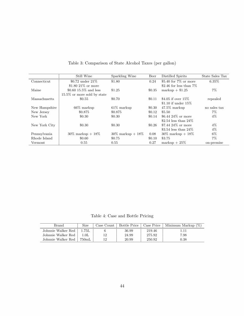
Table 3: Comparison of State Alcohol Taxes (per gallon)

Still Wine Sparkling Wine Beer Distilled Spirits State Sales Tax

Connecticut $0.72 under 21% $1.80 0.24 $5.40 for 7% or more 6.35%$1.80 21% or more $2.46 for less than 7%

Maine $0.60 15.5% and less $1.25 $0.35 markup + $1.25 7%15.5% or more sold by state

Massachusetts $0.55 $0.70 $0.11 $4.05 if over 15% repealed$1.10 if under 15%

New Hampshire 66% markup 61% markup $0.30 47.5% markup no sales taxNew Jersey $0.875 $0.875 $0.12 $5.50 7%New York $0.30 $0.30 $0.14 $6.44 24% or more 4%

$2.54 less than 24%New York City $0.30 $0.30 $0.26 $7.44 24% or more 4%

$3.54 less than 24% 4%Pennsylvania 30% markup + 18% 30% markup + 18% 0.08 30% markup + 18% 6%Rhode Island $0.60 $0.75 $0.10 $3.75 7%Vermont 0.55 0.55 0.27 markup + 25% on-premise

Table 4: Case and Bottle Pricing

Brand Size Case Count Bottle Price Case Price Minimum Markup (%)

Johnnie Walker Red 1.75L 6 36.99 219.46 1.11Johnnie Walker Red 1.0L 12 24.99 275.92 7.98Johnnie Walker Red 750mL 12 20.99 250.92 0.38

44

Table 5: Post and Hold Laws and State Alcohol Consumption

(All) (All) (All) (PH only) (PH NE)

Wine

PH -0.0545*** -0.0623*** -0.0229 -0.0345* -0.00430(0.0183) (0.0183) (0.0192) (0.0190) (0.0340)

R2 0.965 0.966 0.984 0.986 0.984

Beer

PH -0.0155 -0.0283*** -0.0242** -0.0201** -0.0276**(0.0113) (0.0107) (0.0095) (0.0081) (0.0129)

R2 0.891 0.905 0.969 0.960 0.991

Spirits

PH -0.00702 -0.0423** -0.0787*** -0.0854*** -0.0979***(0.0175) (0.0168) (0.0180) (0.0187) (0.0278)

R2 0.950 0.955 0.982 0.976 0.986

Year FE Y Y Y Y YState FE Y Y Y Y YDemog. Controls N Y Y Y YState Time Trends N N Y Y YPH States N N N Y NNE States N N N N YObservations 1,428 1,428 1,428 513 243

Standard errors in parentheses*** p<0.01, ** p<0.05, * p<0.1

Table 6: Post and Hold Laws and Alcohol Retailing

2010 Only All All Northeast

Share of 1-4 Employee Retailers 0.0705 0.0334 0.0454* 0.0466**(0.0436) (0.0209) (0.0262) (0.0227)

R-Squared 0.129 0.868 0.940 0.962

Log(Alcohol Employment/Pop 14+) 0.451 -1.753*** -0.482** -0.431*(0.336) (0.198) (0.240) (0.224)

R-Squared 0.066 0.467 0.739 0.819

Log(Liquor Stores Per Capita) 0.337 -1.336*** -0.599*** -0.514***(0.201) (0.0866) (0.0913) (0.103)

R-Squared 0.149 0.855 0.954 0.963

Obs 51 1275 1275 300Demog Controls Y Y Y Y

State FE N Y Y YYear FE N Y Y Y

State Specific Trends N N Y Y

45

Table 7: Import and Domestic Vodka Share: Northeastern States

Domestic Imported Total Import Share

Connecticut 684,520 440,230 1,124,750 39.1%Massachusetts 1,014,500 1,132,980 2,147,480 52.8%

New Jersey 974,910 1,880,350 2,855,260 65.9%New York 2,256,280 2,759,480 5,015,760 55.0%

Vermont 90,570 45,330 135,900 33.4%New Hampshire 365,940 315,700 681,640 46.3%

Pennsylvania 1,459,740 981,660 2,441,400 40.2%District of Columbia 173,720 186,420 360,140 51.8%

Table 8: Comparison of CT and MA Spirits Sales

QMA × Price -0.0044* -0.0054[ 0.00248] [0.0038]

QMA × Log(Price) -0.107* -0.122[0.0589] [0.0836]

QMA 0.538** 0.761** 0.582** 0.825**[0.071] [0.192] [0.120] [0.284]

PriceCT -1.027** -10.473[0.500] [13.518]

Log(Price) -149.811** -367.300[63.053] [296.424]

Constant 370.027** 803.014** 713.645** 1,574.21*[53.615] [230.663] [348.678] [935.2159]

Type All All Vodka VodkaR2 0.767 0.770 0.733 0.736N 2,705 2,705 713 713

All reported standard errors are heteroskedasticity robust

Table 9: Product Characteristics

Spirit Category Price Proof Products Market Share Total TaxVodka $ 22.39 78.68 405 40.35% $4.13

Rum $18.79 73.68 225 18.90% $3.88Gin $22.15 88.84 65 7.31% $4.65

Tequila $28.90 80.00 114 4.63% $4.20Domestic Whiskey $24.56 81.93 122 11.33% $4.30Imported Whiskey $32.59 81.57 236 17.48% $4.28

Reported Price, Proof and Total Tax are category means weighted by number of units sold. Products is the count ofdistinct brands and sizes. Market Share is the fraction of all of cases sold. Prices are converted to 2013 dollars using

CPI-U.

46

Table 10: Demand Estimates, Logit and Nested Logit, RCNL

(1) (2) (3) (4) (5)Logit LogitIV NLogit NLogitIV RCNL

ρ 0.7939*** 0.8771*** 0.8090***(0.0353) (0.0328) (0.0512)

log(price) -1.8742*** -0.4246 -0.3292*** -1.5570*** -4.886***(0.3745) (1.2910) (0.0797) (0.2319) (0.4621)

σlog p 2.157***(0.312)

σproofgal 0.862***(0.241)

Observations 24,449 24,449 24,449 24,449 24,449R-squared 0.1549 0.1351 0.9454 0.9534 n/aProduct FE 640 640 640 640 640Time FE 52 52 52 52 52

GMM standard errors clustered at product level in parentheses*** p<0.01, ** p<0.05, * p<0.1

Table 11: Price Elasticities by Spirit Category

Spirit Category Mean P25 Median P75

Domestic Whiskey -9.16 -16.3 -11.0 -4.87Gin -9.27 -15.5 -8.65 -5.47Imported Whisky -8.86 -14.9 -6.33 -0.994Rum -11.1 -16.0 -14.2 -6.15Tequila -8.93 -11.7 -5.88 -4.02Vodka -10.6 -16.7 -13.0 -7.64

Aggregate Elasticity Demand -1.05Aggregate Elasticity Consumption -0.957

Mean elasticity is the sales-weighted average elasticity by sprits category.The first, middle and third quartile are reported as P25, Median and P75 respectively

Demand is reported in number of bottles, Consumption is in proof gallons.

47

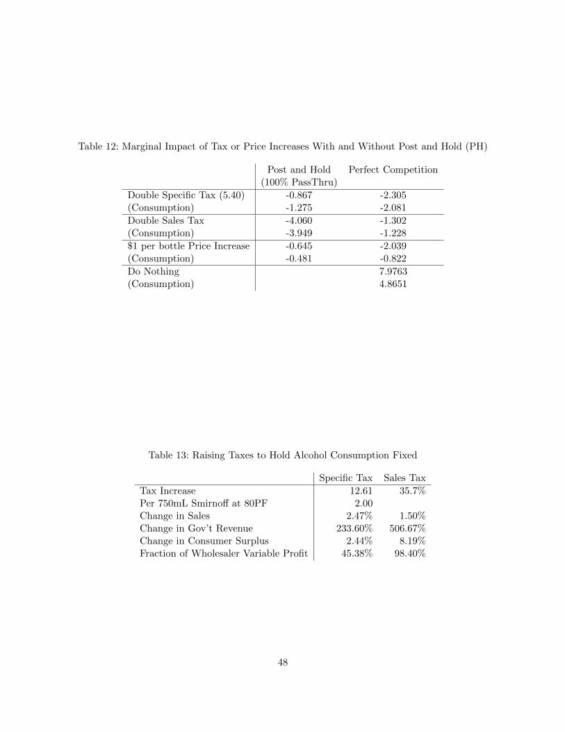
Table 12: Marginal Impact of Tax or Price Increases With and Without Post and Hold (PH)

Post and Hold Perfect Competition(100% PassThru)

Double Specific Tax (5.40) -0.867 -2.305(Consumption) -1.275 -2.081

Double Sales Tax -4.060 -1.302(Consumption) -3.949 -1.228

$1 per bottle Price Increase -0.645 -2.039(Consumption) -0.481 -0.822

Do Nothing 7.9763(Consumption) 4.8651

Table 13: Raising Taxes to Hold Alcohol Consumption Fixed

Specific Tax Sales Tax

Tax Increase 12.61 35.7%Per 750mL Smirnoff at 80PF 2.00Change in Sales 2.47% 1.50%Change in Gov’t Revenue 233.60% 506.67%Change in Consumer Surplus 2.44% 8.19%Fraction of Wholesaler Variable Profit 45.38% 98.40%

48