The Power of Simple Tabulation Hashing

Mihai PatrascuAT&T Labs

Mikkel ThorupAT&T Labs

May 10, 2011

Abstract

Randomized algorithms are often enjoyed for their simplicity, but the hash functions usedto yield the desired theoretical guarantees are often neither simple nor practical. Here we showthat the simplest possible tabulation hashing provides unexpectedly strong guarantees.

The scheme itself dates back to Carter and Wegman (STOC’77). Keys are viewed as consist-ing of c characters. We initialize c tables T1, . . . , Tc mapping characters to random hash codes.A key x = (x1, . . . , xc) is hashed to T1[x1]⊕ · · · ⊕ Tc[xc], where ⊕ denotes xor.

While this scheme is not even 4-independent, we show that it provides many of the guaranteesthat are normally obtained via higher independence, e.g., Chernoff-type concentration, min-wisehashing for estimating set intersection, and cuckoo hashing.

Contents

1 Introduction 2

2 Concentration Bounds 7

3 Linear Probing and the Concentration in Arbitrary Intervals 13

4 Cuckoo Hashing 19

5 Minwise Independence 27

6 Fourth Moment Bounds 32

A Experimental Evaluation 39

B Chernoff Bounds with Fixed Means 46

1

arX

iv:1

011.

5200

v2 [

cs.D

S] 7

May

201

1

1 Introduction

An important target of the analysis of algorithms is to determine whether there exist practicalschemes, which enjoy mathematical guarantees on performance.

Hashing and hash tables are one of the most common inner loops in real-world computation, andare even built-in “unit cost” operations in high level programming languages that offer associativearrays. Often, these inner loops dominate the overall computation time. Knuth gave birth tothe analysis of algorithms in 1963 [Knu63] when he analyzed linear probing, the most popularpractical implementation of hash tables. Assuming a perfectly random hash function, he boundedthe expected number of probes. However, we do not have perfectly random hash functions. Theapproach of algorithms analysis is to understand when simple and practical hash functions workwell. The most popular multiplication-based hashing schemes maintain the O(1) running timeswhen the sequence of operations has sufficient randomness [MV08]. However, they fail badly evenfor very simple input structures like an interval of consecutive keys [PPR09, PT10, TZ09], givinglinear probing an undeserved reputation of being non-robust.

On the other hand, the approach of algorithm design (which may still have a strong elementof analysis) is to construct (more complicated) hash functions providing the desired mathemati-cal properties. This is usually done in the influential k-independence paradigm of Wegman andCarter [WC81]. It is known that 5-independence is sufficient [PPR09] and necessary [PT10] for lin-ear probing. Then one can use the best available implementation of 5-independent hash functions,the tabulation-based method of [TZ04,TZ09].

Here we analyze simple tabulation hashing. This scheme views a key x as a vector of c charactersx1, . . . , xc. For each character position, we initialize a totally random table Ti, and then use thehash function

h(x) = T1[x1]⊕ · · · ⊕ Tc[xc].

This is a well-known scheme dating back at least to Wegman and Carter [WC81]. From a practicalview-point, tables Ti can be small enough to fit in fast cache, and the function is probably theeasiest to implement beyond the bare multiplication. However, the scheme is only 3-independent,and was therefore assumed to have weak mathematical properties. We note that if the keys aredrawn from a universe of size u, and hash values are machine words, the space required is O(cu1/c)words. The idea is to make this fit in fast cache. We also note that the hash values are bit strings,so when we hash into bins, the number of bins is generally understood to be a power of two.

The challenge in analyzing simple tabulation is the significant dependence between keys. Nev-ertheless, we show that the scheme works in some of the most important randomized algorithms,including linear probing and several instances when Ω(lg n)-independence was previously needed.We confirm our findings by experiments: simple tabulation is competitive with just one 64-bitmultiplication, and the hidden constants in the analysis appear to be very acceptable in practice.

In many cases, our analysis gives the first provably good implementation of an algorithm whichmatches the algorithm’s conceptual simplicity if one ignores hashing.

Desirable properties. We will focus on the following popular properties of truly random hashfunctions.

• The worst-case query time of chaining is O(lg n/ lg lg n) with high probability (w.h.p.). Moregenerally, when distributing balls into bins, the bin load obeys Chernoff bounds.

• Linear probing runs in expected O(1) time per operation. Variance and all constant momentsare also O(1).

2

• Cuckoo hashing: Given two tables of size m ≥ (1 + ε)n, it is possible to place a ball in one oftwo randomly chosen locations without any collision, with probability 1−O( 1

n).

• Given two sets A,B, we have Prh[minh(A) = minh(B)] = |A∩B||A∪B| . This can be used to quickly

estimate the intersection of two sets, and follows from a property called minwise independence:for any x /∈ S, Prh[x < minh(S)] = 1

|S|+1 .

As defined by Wegman and Carter [WC81] in 1977, a family H = h : [u] → [m] of hashfunctions is k-independent if for any distinct x1, . . . , xk ∈ [u], the hash codes h(x1), . . . , h(xk) areindependent random variables, and the hash code of any fixed x is uniformly distributed in [m].

Chernoff bounds continue to work with high enough independence [SSS95]; for instance, in-dependence Θ( lgn

lg lgn) suffices for the bound on the maximum bin load. For linear probing, 5-independence is sufficient [PPR09] and necessary [PT10]. For cuckoo hashing, O(lg n)-independencesuffices and at least 6-independence is needed [CK09]. While minwise independence cannotbe achieved, one can achieve ε-minwise independence with the guarantee (∀)x /∈ S,Prh[x <minh(S)] = 1±ε

|S|+1 . For this, Θ(lg 1ε ) independence is sufficient [Ind01] and necessary [PT10]. (Note

that the ε is a bias so it is a lower bound on how well set intersection can be approximated, withany number of independent experiments.)

The canonical construction of k-independent hash functions is a random degree k−1 polynomialin a prime field, which has small representation but Θ(k) evaluation time. Competitive implemen-tations of polynomial hashing simulate arithmetic modulo Mersenne primes via bitwise operations.Even so, tabulation-based hashing with O(u1/c) space and O(ck) evaluation time is significantlyfaster [TZ04]. The linear dependence on k is problematic, e.g., when k ≈ lg n.

Siegel [Sie04] shows that a family with superconstant independence but O(1) evaluation time re-quires Ω(uε) space, i.e. it requires tabulation. He also gives a solution that uses O(u1/c) space, cO(c)

evaluation time, and achieves uΩ(1/c2) independence (which is superlogarithmic, at least asymptot-ically). The construction is non-uniform, assuming a certain small expander which gets used ina graph product. Dietzfelbinger and Rink [DR09] use universe splitting to obtain similar highindependence with some quite different costs. Instead of being highly independent on the wholeuniverse, their goal is to be highly independent on an unknown but fixed set S of size n. For someconstant parameter γ, they tolerate an error probability of n−γ . Assuming no error, their hashfunction is highly independent on S. The evaluation time is constant and the space is sublinear.For error probability n−γ , each hash computation calls O(γ) subroutines, each of which evaluatesits own degree O(γ) polynomial. The price for a lower error tolerance is therefore a slower hashfunction (even if we only count it as constant time in theory).

While polynomial hashing may perform better than its independence suggests, we have nopositive example yet. On the tabulation front, we have one example of a good hash function thatis not formally k-independent: cuckoo hashing works with an ad hoc hash function that combinesspace O(n1/c) and polynomials of degree O(c) [DW03].

1.1 Our results

Here we provide an analysis of simple tabulation showing that it has many of the desirable propertiesabove. For most of our applications, we want to rule out certain obstructions with high probability.This follows immediately if certain events are independent, and the algorithms design approach isto pick a hash function guaranteeing this independence, usually in terms of a highly independenthash function.

3

Instead we here stick with simple tabulation with all its dependencies. This means that we haveto struggle in each individual application to show that the dependencies are not fatal. However,from an implementation perspective, this is very attractive, leaving us with one simple and fastscheme for (almost) all our needs.

In all our results, we assume the number of characters is c = O(1). The constants in ourbounds will depend on c. Our results use a rather diverse set of techniques analyzing the tabledependencies in different types of problems. For chaining and linear probing, we rely on someconcentration results, which will also be used as a starting point for the analysis of min-wisehashing. Theoretically, the most interesting part is the analysis for cuckoo hashing, with a veryintricate study of the random graph constructed by the two hash functions.

Chernoff bounds. We first show that simple tabulation preserves Chernoff-type concentration:

Theorem 1. Consider hashing n balls into m ≥ n1−1/(2c) bins by simple tabulation. Let q be anadditional query ball, and define Xq as the number of regular balls that hash into a bin chosen asa function of h(q). Let µ = E[Xq] = n

m . The following probability bounds hold for any constant γ:

(∀)δ ≤ 1 : Pr[|Xq − µ| > δµ] < 2e−Ω(δ2µ) +m−γ (1)

(∀)δ = Ω(1) : Pr[Xq > (1 + δ)µ] < (1 + δ)−Ω((1+δ)µ) +m−γ (2)

With m ≤ n bins, every bin gets

n/m±O(√

n/m logc n). (3)

keys with probability 1− n−γ.

Contrasting standard Chernoff bounds (see, e.g., [MR95]), Theorem 1 can only provide polyno-mially small probability, i.e. at least n−γ for any desired constant γ. In addition, the exponentialdependence on µ in (1) and (2) is reduced by a constant which depends (exponentially) on the con-stants γ and c. It is possible to get some super polynomially small bounds with super constant γ butthey are not as clean. An alternative way to understand the bound is that our tail bound dependsexponentially on εµ, where ε decays to subconstant as we move more than inversely polynomialout in the tail. Thus, our bounds are sufficient for any polynomially high probability guarantee.However, compared to the standard Chernoff bound, we would have to tolerate a constant factormore balls in a bin to get the same failure probability.

By the union bound (1) implies that with m = Θ(n) bins, no bin receives more thanO(lg n/ lg lg n) balls w.h.p. This is the first realistic hash function to achieve this fundamentalproperty. Similarly, for linear probing with fill bounded below 1, (2) shows that the longest filledinterval is of length O(log n) w.h.p.

Linear probing. Building on the above concentration bounds, we show that if the table size ism = (1 + ε)n, then the expected time per operation is O(1/ε2), which asymptotically matches thebound of Knuth [Knu63] for a truly random function. In particular, this compares positively withthe O(1/ε13/6) bound of [PPR09] for 5-independent hashing.

Our proof is a combinatorial reduction that relates the performance of linear probing to concen-tration bounds. The results hold for any hash function with concentration similar to Theorem 1.To illustrate the generality of the approach, we also improve the O(1/ε13/6) bound from [PPR09]for 5-independent hashing to the optimal O(1/ε2). This was raised as an open problem in [PPR09].

4

For simple tabulation, we get quite strong concentration results for the time per operation, e.g,,constant variance for constant ε. For contrast, with 5-independent hashing, the variance is onlyknown to be O(log n) [PPR09,TZ09].

Cuckoo hashing. In general, the cuckoo hashing algorithm fails iff the random bipartite graphinduced by two hash functions contains a component with more vertices than edges. With trulyrandom hashing, this happens with probability Θ( 1

n). Here we study the random graphs induced bysimple tabulation, and obtain a rather unintuitive result: the optimal failure probability is inverselyproportional to the cube root of the set size.

Theorem 2. Any set of n keys can be placed in two table of size m = (1+ε) by cuckoo hashing andsimple tabulation with probability 1−O(n−1/3). There exist sets on which the failure probability isΩ(n−1/3).

Thus, cuckoo hashing and simple tabulation are an excellent construction for a static dictionary.The dictionary can be built (in linear time) after trying O(1) independent hash functions w.h.p.,and later every query runs in constant worst-case time with two probes. We note that even thoughcuckoo hashing requires two independent hash functions, these essentially come for the cost of onein simple tabulation: the pair of hash codes can be stored consecutively, in the same cache line,making the running time comparable with evaluating just one hash function.

In the dynamic case, Theorem 2 implies that we expect Ω(n4/3) updates between failures re-quiring a complete rehash with new hash functions.

Our proof involves a complex understanding of the intricate, yet not fatal dependencies in simpletabulation. The proof is a (complicated) algorithm that assumes that cuckoo hashing has failed,and uses this knowledge to compress the random tables T1, . . . , Tc below the entropy lower bound.

Using our techniques, it is also possible to show that if n balls are placed in O(n) bins inan online fashion, choosing the least loaded bin at each time, the maximum load is O(lg lg n) inexpectation.

Minwise independence. In the full version, we show that simple tabulation is ε-minwise in-dependent, for a vanishingly small ε (inversely polynomial in the set size). This would requireΘ(log n) independence by standard techniques.

Theorem 3. Consider a set S of n = |S| keys and q /∈ S. Then with h implemented by simpletabulation:

Pr[h(q) < minh(S)] =1± εn

, where ε = O

(lg2 n

n1/c

).

This can be used to estimate the size of set intersection by estimating:

Pr[minh(A) = minh(B)]

=∑

x∈A∩BPr[x < minh(A ∪B \ x)]

=|A ∩B||A ∪B|

·(

1± O(

1

|A ∪B|1/c

)).

For good bounds on the probabilities, we would make multiple experiments with independent hashfunctions. An alternative based on a single hash function is that we for each set consider the

5

k elements with the smallest hash values. We will also present concentration bounds for thisalternative.

Fourth moment bounds. An alternative to Chernoff bounds in proving good concentration isto use bounded moments. In the full version of the paper, we analyze the 4th moment of a bin’ssize when balls are placed into bins by simple tabulation. For a fixed bin, we show that the 4th

moment comes extremely close to that achieved by truly random hashing: it deviates by a factorof 1 + O(4c/m), which is tiny except for a very large number of characters c. This would require4-independence by standard arguments. This limited 4th moment for a given bin was discoveredindependently by [BCL+10].

If we have a designated query ball q, and we are interested in the size of a bin chosen as afunction of h(q), the 4th moment of simple tabulation is within a constant factor of that achievedby truly random hashing (on close inspection of the proof, that constant is at most 2). This wouldrequire 5-independence by standard techniques. (See [PT10] for a proof that 4-independence canfail quite badly when we want to bound the size of the bin in which q lands.) Our proof exploitsan intriguing phenomenon that we identify in simple tabulation: in any fixed set of 5 keys, one ofthem has a hash code that is independent of the other four’s hash codes.

Unlike our Chernoff-type bounds, the constants in the 4th moment bounds can be analyzed quiteeasily, and are rather tame. Compelling applications of 4th moment bounds were given by [KR93]and [Tho09]. In [KR93], it was shown that any hash function with a good 4th moment boundsuffices for a nonrecursive version of quicksort, routing on the hypercube, etc. In [Tho09], linearprobing is shown to have constant expected performance if the hash function is a composition ofuniversal hashing down to a domain of size O(n), with a strong enough hash function on this smalldomain (i.e. any hash function with a good 4th moment bound).

We will also use 4th moment bounds to attain certain bounds of linear probing not covered byour Chernoff-type bounds. In the case of small fill α = n

m = o(1), we use the 4th moment boundsto show that the probability of a full hash location is O(α).

Pseudorandom numbers. The tables used in simple tabulation should be small to fit in thefirst level of cache. Thus, filling them with truly random numbers would not be difficult (e.g. inour experiments we use atmospheric noise from random.org). If the amount of randomness needsto be reduced further, we remark that all proofs continue to hold if the tables are filled by aΘ(lg n)-independent hash function (e.g. a polynomial with random coefficients).

With this modification, simple tabulation naturally lends itself to an implementation of a veryefficient pseudorandom number generator. We can think of a pseudorandom generator as a hashfunction on range [n], with the promise that each h(i) is evaluated once, in the order of increasing i.To use simple tabulation, we break the universe into two, very lopsided characters: [ nR ]× [R], for Rchosen to be Θ(lg n). Here the second coordinate is least significant, that is, (x, y) represents xR+y.During initialization, we fill T2[1 . . R] with R truly random numbers. The values of T1[1 . . n/R] aregenerated on the fly, by a polynomial of degree Θ(lg n), whose coefficients were chosen randomlyduring initialization. Whenever we start a new row of the matrix, we can spend a relatively largeamount of time to evaluate a polynomial to generate the next value r1 which we store in a register.For the next R calls, we run sequentially through T2, xoring each value with r1 to provide a newpseudorandom number. With T2 fitting in fast memory and scanned sequentially, this will bemuch faster than a single multiplication, and with R large, the amortized cost of generating r1

is insignificant. The pseudorandom generator has all the interesting properties discussed above,including Chernoff-type concentration, minwise independence, and random graph properties.

6

Experimental evaluation. We performed an experimental evaluation of simple tabulation. Ourimplementation uses tables of 256 entries (i.e. using c = 4 characters for 32-bit data and c = 8characters with 64-bit data). The time to evaluate the hash function turns out to be competitivewith multiplication-based 2-independent functions, and significantly better than for hash functionswith higher independence. We also evaluated simple tabulation in applications, in an effort toverify that the constants hidden in our analysis are not too large. Simple tabulation proved veryrobust and fast, both for linear probing and for cuckoo hashing.

Notation. We now introduce some notation that will be used throughout the proofs. We wantto construct hash functions h : [u] → [m]. We use simple tabulation with an alphabet of Σ andc = O(1) characters. Thus, u = Σc and h(x1, . . . , xc) =

⊕ci=1 Ti[xi]. It is convenient to think of

each hash code Ti[xi] as a fraction in [0, 1) with large enough precision. We always assume m is apower of two, so an m-bit hash code is obtained by keeping only the most significant log2m bitsin such a fraction. We always assume the table stores long enough hash codes, i.e. at least log2mbits.

Let S ⊂ Σc be a set of |S| = n keys, and let q be a query. We typically assume q /∈ S, sincethe case q ∈ S only involves trivial adjustments (for instance, when looking at the load of the binh(q), we have to add one when q ∈ S). Let π(S, i) be the projection of S on the i-th coordinate,π(S, i) = xi | (∀)x ∈ S.

We define a position-character to be an element of [c] × Σ. Then, the alphabets on eachcoordinate can be assumed to be disjoint: the first coordinate has alphabet 1×Σ, the second hasalphabet 2 × Σ, etc. Under this view, we can treat a key x as a set of q position-characters (ondistinct positions). Furthermore, we can assume h is defined on position characters: h((i, α)) =Ti[α]. This definition is extended to keys (sets of position-characters) in the natural way h(x) =⊕

α∈x h(α).When we say with high probability in r, we mean 1 − ra for any desired constant a. Since

c = O(1), high probability in |Σ| is also high probability in u. If we just say high probability, it isunderstood to be in n.

2 Concentration Bounds

This section proves Theorem 1, except branch (3) which is shown in the full version of the paper.If n elements are hashed into n1+ε bins by a truly random hash function, the maximum load of

any bin is O(1) with high probability. First we show that simple tabulation preserves this guarantee.Building on this, we shows that the load of any fixed bin obeys Chernoff bounds. Finally we showthat the Chernoff bound holds even for a bin chosen as a function of the query hash code, h(q).

As stated in the introduction, the number of bins is always understood to be a power of two.This is because our hash values are xor’ed bit strings. If we want different numbers of bins we couldview the hash values as fractions in the unit interval and divide the unit interval into subintervals.Translating our results to this setting is standard.

2.1 Hashing into Many Bins

The notion of peeling lies at the heart of most work in tabulation hashing. If a key from a set ofkeys contains one position-character that doesn’t appear in the rest of the set, its hash code will beindependent of the rest. Then, it can be “peeled” from the set, as its behavior matches that with

7

truly random hashing. More formally, we say a set T of keys is peelable if we can arrange the keysof T in some order, such that each key contains a position-character that doesn’t appear amongthe previous keys in the order.

Lemma 4. Suppose we hash n ≤ m1−ε keys into m bins, for some constant ε > 0. For anyconstant γ, all bins get less than d = min

((1 + γ)/ε)c , 2(1+γ)/ε

keys with probability ≥ 1−m−γ.

Proof. We will show that among any d elements, one can find a peelable subset of size t ≥maxd1/c, lg d. Then, a necessary condition for the maximum load of a bin to be at least d isthat some bin contain t peelable elements. There are at most

(nt

)< nt such sets. Since the hash

codes of a peelable set are independent, the probability that a fixed set lands into a common binis 1/mt−1. Thus, an upper bound on the probability that the maximum load is d can be obtained:

nt/mt−1 = m(1−ε)t/mt−1 = m1−εt. To obtain failure probability m−γ , set t = (1 + γ)/ε.It remains to show that any set T of |T | = d keys contains a large peelable subset. Since

T ⊂ π(T, 1) × · · · × π(T, c), it follows that there exists i ∈ [c] with |π(T, i)| ≥ d1/c. Pick someelement from T for every character value in π(S, i); this is a peelable set of t = d1/c elements.

To prove t ≥ log2 d, we proceed iteratively. Consider the coordinate giving the largest projection,j = arg maxi |π(T, i)|. As long as |T | ≥ 2, |π(T, j)| ≥ 2. Let α be the most popular value in Tfor the j-th character, and let T ? contain only elements with α on the j-th coordinate. We have|T ?| ≥ |T |/|π(T, j)|. In the peelable subset, we keep one element for every value in π(T, j) \ α,and then recurse in T ? to obtain more elements. In each recursion step, we obtain k ≥ 1 elements,at the cost of decreasing log2 |T | by log2(k+1). Thus, we obtain at least log2 d elements overall.

We note that, when the subset of keys of interest forms a combinatorial cube, the probabilisticanalysis in the proof is sharp up to constant factors. In other words, the exponential dependenceon c and γ is inherent.

2.2 Chernoff Bounds for a Fixed Bin

We study the number of keys ending up in a prespecified bin B. The analysis will define a totalordering ≺ on the space of position-characters, [c] × Σ. Then we will analyze the random processby fixing hash values of position-characters h(α) in the order ≺. The hash value of a key x ∈ Sbecomes known when the position-character max≺ x is fixed. For α ∈ [c]× Σ, we define the groupGα = x ∈ S | α = max≺ x, the set of keys for whom α is the last position-character to be fixed.

The intuition is that the contribution of each group Gα to the bin B is a random variableindependent of the previous Gβ’s, since the elements Gα are shifted by a new hash code h(α).Thus, if we can bound the contribution of Gα by a constant, we can apply Chernoff bounds.

Lemma 5. There is an ordering ≺ such that the maximal group size is maxα |Gα| ≤ n1−1/c.

Proof. We start with S being the set of all keys, and reduce S iteratively, by picking a position-character α as next in the order, and removing keys Gα from S. At each point in time, we pick theposition-character α that would minimize |Gα|. Note that, if we pick some α as next in the order,Gα will be the set of keys x ∈ S which contain α and contain no other character that hasn’t beenfixed: (∀)β ∈ x \ α, β ≺ α.

We have to prove is that, as long as S 6= ∅, there exists α with |Gα| ≤ |S|1−1/c. If some positioni has |π(S, i)| > |S|1/c, there must be some character α on position i which appears in less than|S|1−1/c keys; thus |Gα| ≤ S1−1/c. Otherwise, π(S, i) ≤ |S|1/c for all i. Then if we pick an arbitrarycharacter α on some position i, have |Gα| ≤

∏j 6=i |π(S, j)| ≤ (|S|1/c)c−1 = |S|1−1/c.

8

From now on assume the ordering ≺ has been fixed as in the lemma. This ordering partitionsS into at most n non-empty groups, each containing at most n1−1/c keys. We say a group Gα isd-bounded if no bin contains more than d keys from Gα.

Lemma 6. Assume the number of bins is m ≥ n1−1/(2c). For any constant γ, with probability≥ 1−m−γ, all groups are d-bounded where

d = min

(2c(3 + γ)c, 22c(3+γ)

Proof. Since |Gα| ≤ n1−1/c ≤ m1−1/(2c), by Lemma 4, we get that there are at most d keys fromGα in any bin with probability 1−m−(2+γ) ≥ 1−m−γ/n. The conclusion follows by union boundover the ≤ n groups.

Henceforth, we assume that γ and d are fixed as in Lemma 6. Chernoff bounds (see [MR95,Theorem 4.1]) consider independent random variables X1, X2, · · · ∈ [0, d]. Let X =

∑iXi, µ =

E[X], and δ > 0, the bounds are:

Pr[X ≥ (1 + δ)µ] ≤(

eδ

(1 + δ)(1+δ)

)µ/dPr[X ≤ (1− δ)µ] ≤

(e−δ

(1− δ)(1−δ)

)µ/d (4)

Let Xα be the number of elements from Gα landing in the bin B. We are quite close to applyingChernoff bounds to the sequence Xα, which would imply the desired concentration around µ = n

m .Two technical problems remain: Xα’s are not d-bounded in the worst case, and they are notindependent.

To address the first problem, we define the sequence of random variables Xα as follows: ifGα is d-bounded, let Xα = Xα; otherwise Xα = |Gα|/m is a constant. Observe that

∑α Xα

coincides with∑

αXα if all groups are d-bounded, which happens with probability 1−m−γ . Thus

a probabilistic bound on∑

α Xα is a bound on∑

αXα up to an additive m−γ in the probability.

Finally, the Xα variables are not independent: earlier position-character dictate how keys clus-ter in a later group. Fortunately (4) holds even if the distribution of each Xi is a function ofX1, . . . , Xi−1, as long as the mean E[Xi | X1, . . . , Xi−1] is a fixed constant µi independent ofX1, ..., Xi−1. A formal proof will be given in Appendix B. We claim that our means are fixed thisway: regardless of the hash codes for β < α, we will argue that E[Xα] = µα = |Gα|/m.

Observe that whether or not Gα is d-bounded is determined before h(α) is fixed in the order ≺.Indeed, α is the last position-character to be fixed for any key in Gα, so the hash codes of all keysin Gα have been fixed up to an xor with h(α). This final shift by h(α) is common to all the keys,so it cannot change whether or not two elements land together in a bin. Therefore, the choice ofh(α) does not change if Gα is d-bounded.

After fixing all hash codes β ≺ α, we decide if Gα is d-bounded. If not, we set Xα = |Gα|/m.Otherwise Xα = Xα is the number of elements we get in B when fixing h(α), and h(α) is a uniformrandom variable sending each element to B with probability 1/m. Therefore E[Xα] = |Gα|/m.This completes the proof that the number of keys in bin B obeys Chernoff bounds from (4), whichimmediately imply (1) and (2) in Theorem 1.

9

2.3 The Load of a Query-Dependent Bin

When we are dealing with a special key q (a query), we may be interested in the load of a binBq, chosen as a function of the query’s hash code, h(q). We show that the above analysis alsoworks for the size of Bq, up to small constants. The critical change is to insist that the queryposition-characters come first in our ordering ≺:

Lemma 7. There is an ordering ≺ placing the characters of q first, in which the maximal groupsize is 2 · n1−1/c.

Proof. After placing the characters of q at the beginning of the order, we use the same iterativeconstruction as in Lemma 5. Each time we select the position-character α minimizing |Gα|, place αnext in the order ≺, and remove Gα from S. It suffices to prove that, as long as S 6= ∅, there existsa position-character α /∈ q with |Gα| ≤ 2 · |S|1−1/c. Suppose in some position i, |π(S, i)| > |S|1/c.Even if we exclude the query character qi, there must be some character α on position i thatappears in at most |S|/(|π(S, i)| − 1) keys. Since S 6= ∅, |S|1/c > 1, so |π(S, i)| ≥ 2. This means|π(S, i)| − 1 ≥ |S|1/c/2, so α appears in at most 2|S|1−1/c keys. Otherwise, we have π(S, i) ≤ |S|1/cfor all i. Then, for any character α on position i, we have |Gα| ≤

∏j 6=i |π(S, j)| ≤ |S|1−1/c.

The lemma guarantees that the first nonempty group contains the query alone, and all latergroups have random shifts that are independent of the query hash code. We lost a factor twoon the group size, which has no effect on our asymptotic analysis. In particular, all groups ared-bounded w.h.p. Letting Xα be the contribution of Gα to bin Bq, we see that the distribution ofXα is determined by the hash codes fixed previously (including the hash code of q, fixing the choiceof the bin Bq). But E[Xα] = |Gα|/m holds irrespective of the previous choices. Thus, Chernoffbounds continue to apply to the size of Bq. This completes the proof of (1) and (2) in Theorem 1.

In Theorem 1 we limited ourselves to polynomially small error bounds m−γ for constant γ.However, we could also consider a super constant γ = ω(1) using the formula for d in Lemma 6.For the strongest error bounds, we would balance m−γ with the Chernoff bounds from (4). Suchbalanced error bounds would be messy, and we found it more appealing to elucidate the standardChernoff-style behavior when dealing with polynomially small errors.

2.4 Few bins

We will now settle Theorem 1 (3), proving some high probability bounds for the concentration withm ≤ n bins. As stated in (3), we will show, w.h.p., that the number of keys in each bin is

n/m±O(√n/m logc n).

Consider any subset S of s ≤ n keys that only vary in b characters. Generalizing (3), we will showfor any L ≥ 32 log n, that with probability 1− exp(−Ω(L)), the keys in S get distributed with

s/m±√s/mLb if s ≥ mLb/2

≤ Lb if s ≤ mLb/2 (5)

keys in each of the m bins. This is trivial for m = 1, so we can assume m ≥ 2. The proof is byinduction on (b, s). First we will prove that each inductive step fails with small probability. Laterwe will conclude that the combined failure probability for the whole induction is small.

10

For the base case of the induction, if s ≤ Lb, the result is trivial since it holds even if some bingets all the keys from S. This case includes if we have no characters to vary, that is, when s = 1and b = 0. We may therefore assume that s > Lb, and b > 0. The characters positions where S donot vary will only shuffle the bins, but not affect which keys from S go together, so we can ignorethem when giving bounds for the sizes of all bins.

Considering the varying characters in S, we apply the ordering from Section 2.2 leading to agrouping of S. By Lemma 5, there is an ordering ≺ such that the maximal group size is maxα |Gα| ≤s1−1/b. In particular, maxα |Gα| < s/L.

First, assume that s ≤ mLb/2. Each group has one less free character, so by induction, eachgroup has at most Lb−1 keys in each bin, that is, each group is Lb−1-bounded. Now as in Section 2.2,for any fixed bin, we can apply the Chernoff upper-bound from (4) with d = Lb−1. We haveµ = s/m ≤ Lb/2, and we want to bound the probability of getting a bin of size at least x = Lb ≥ 2µ.For an upper bound, we use µ′ = x/2 ≥ µ and δ′ = 1, and get a probability bound of(

eδ′

(1 + δ′)(1+δ′)

)µ′/d= (e/4)µ

′/d ≤ (e/4)L/2.

With the union bound, the probability that any bin has more than Lb keys is bounded by m(e/4)L/2.

Partitioning many keys. Next, we consider the more interesting case where s ≥ mLb/2. Asstated in (5), we want to limit the probability that the contribution S to any bin deviates by morethan

√s/mLb from the mean s/m. We partition the groups into levels i based on their sizes. On

level 0 we have the groups of size up to mLb−1/2. On level i > 0, we have the groups of sizebetween ti = mLb−12i−2 and 2ti. For each i, we let Si denote the union of the level i groups. Weare going to handle each level i separately, providing a high probability bound on how much thecontribution of Si to a given bin can deviate from the mean. Adding the deviations from all levels,we bound the total deviation in the contribution from S to this bin. Let si be the number of keysin Si and define

∆i =√si/mLb−1/2. (6)

For level i > 0, we will use ∆i as our deviation bound, while we for i = 0, will use ∆0 = max∆0, Lb.

The total deviation. We will now show that the above level deviation bounds provide thedesired total deviation bound of

√s/mLb from (5). Summing over the levels, the total deviation is

bounded by Lb +∑

i

√si/mLb−1/2. To bound the sum, we first consider the smaller terms where

si < s/ log n. Then√si/mL

b−1/2 ≤√s/mLb/

√L log n. We have at most logn values of i, so these

smaller terms sum to at most√s/mLb

√(log n)/L.

Next we consider the larger terms where si ≥ s/ log n. Each such term can be bounded as√si/mLb−1/2 =

((si/m)/

√si/m

)Lb−1/2

≤(

(si/m)/√s/m

)Lb√

log n/L.

The sum of the larger terms is therefore also bounded by√s/mLb

√(log n)/L. Thus the

total deviation is bounded by Lb +√s/mLb2

√(log n)/L. Assuming L ≥ 9 log n, we have

2√

(log n)/L ≤ 2/3. Moreover, with n ≥ 4 and b ≥ 1, we have s/m > Lb/2 ≥ 9. It followsthat Lb + 2

√(log n)/L

√s/mLb ≤

√s/mLb, as desired.

11

Deviation from small groups. We now consider the contribution to our bin from the smallgroups in S0. These groups have size most (mLb/2)1−1/b ≤ mLb−1/2, and b − 1 free characterpositions, so inductively from (5), each group contributes at most d0 ≤ Lb−1 to each bin. We wantto bound the probability that the deviation from the mean µ0 = s0/m exceeds ∆0 = max∆0, L

b.Suppose µ0 ≤ ∆0. For a Chernoff upper bound, we use µ′ = ∆0 ≥ µ0 and δ′ = 1, and get a

probability bound of (eδ′/(1 + δ′)(1+δ′)

)µ′/d0

= (e/4)µ′/d0 ≤ (e/4)L.

On the other hand, if µ0 ≥ ∆0, we have a relative deviation of δ0 = ∆0/µ0 =√m/s0L

b−1/2 ≤ 1.The probability of this deviation for any fixed bin is bounded by(

eδ0/(1 + δ0)(1+δ0))µ0/d0

≤ exp(−(µ0/d0)δ20/3) = exp(−Lb/3) ≤ exp(−L/3).

Larger groups. To deal with a larger group level i > 1, we will use a standard symmetric Chernoffbound, which is easily derived from the negative version of (4). We consider independent n randomvariables X1, ...., Xn ∈ [−d, d], each with mean zero. Let X =

∑iXi. For any δ > 0,

Pr[|X| ≥ δdn] ≤ 2 exp(−nδ2/4) (7)

As we did for (4) in Section 2.2, we note that (7) also holds when Xi depends on the previous Xj ,j < i, as long as |Xi| ≤ d and E[Xi] = 0. Back to our problem, let si be the total size. Each groupG has size at least ti = mLb−12i−2, so we have at most ni = si/ti groups. The group G has onlyb− 1 varying characters and ti ≥ t1 = mLb−1/2, so inductively from (5), the contribution of G toany bin deviates by at most di =

√|G|/mLb−1 <

√2ti/mL

b−1 from the mean |G|/m. We let XG

denote the contribution of G to our bin minus the mean |G|/m. Thus, regardless of the distributionof previous groups, we have E[XG] = 0 and |XG| ≤ di. We want to bound the probability that|∑

GX| ≥ ∆i. We therefore apply (7) with

δi = ∆i/(dini) =√si/mLb−1/2/

(√2ti/mL

b−1si/ti

)=√tiL/(2si).

The probability that the contribution to our bin deviates by more than ∆i is therefore bounded by

2 exp(−niδ2i /4) = 2 exp(−si/ti ·

√tiL/(2si)

2/4) = 2 exp(−L/8).

Conveniently, this dominates the error probabilities of (e/4)L and exp(−L/3) from level 0. Thereare less log n levels, so by the union bound, the probability of a too large deviation from any levelto any bin is bounded by m(log n)2 exp(−L/8).

Error probability for the whole induction. Above we proved that any particular inductivestep fails with probability at most m(log n)2 exp(−L/8). We want to conclude that the probabilityof any failure in the whole induction is bounded by nm exp(−L/8).

First we note that the all the parameters of the inductive steps are determined deterministically.More precisely, the inductive step is defined via the deterministic grouping from Lemma 5. Thisgrouping corresponds to a certain deterministic ordering of the position characters, and we usethis ordering to analyze the failure probability of the inductive step. However, there is no relationbetween the ordering used to analyze different inductive steps. Thus, we are dealing with a recursive

12

deterministic partitioning. Each partitioning results in groups that are at least L times smaller,so the recursion corresponds to a tree with degrees at least L. At the bottom we have base cases,each containing at least one key. The internal nodes correspond to inductive steps, so we have lessthan 2n/L of these. If L ≥ 4 log n, we conclude that the combined failure probability is at most2n/Lm(log n)2 exp(−L/8) ≤ nm exp(−L/8). With L ≥ 32 log n, we get that the overall failureprobability is bounded by exp(−L/64). This completes our proof that (5) is satisfied with highprobability, hence the proof of Theorem 1 (3).

3 Linear Probing and the Concentration in Arbitrary Intervals

We consider linear probing using simple tabulation hashing to store a set S of n keys in an array ofsize m (as in the rest of our analyses, m is a power of two). Let α = 1− ε = n

m be the fill. We willargue that the performance with simple tabulation is within constant factors of the performancewith a truly random function, both in the regime ε ≥ 1/2 (high fill) and α ≤ 1/2 (low fill). Withhigh fill, the expected number of probes when we insert a new key is O(1/ε2) and with low fill, itis 1 +O(α).

Pagh et al. [PPR09] presented an analysis of linear probing with 5-independent hashing using4th moment bounds. They got a bound of O(1/ε13/6) on the expected number of probes. We feelthat our analysis, which is centered around dyadic intervals, is simpler, tighter, and more generic.Recall that a dyadic interval, is an interval of the form [j2i, (j + 1)2i) for integers i and j. In fact,as we shall see later in Section 6.4, our analysis also leads to an optimal O(1/ε2) for 5-independenthashing, settling an open problem from [PPR09]. However, with simple tabulation, we get muchstronger concentration than with 5-independent hashing, e.g., constant variance with constant εwhereas the variance is only known to be O(log n) with 5-independent hashing.

When studying the complexity of linear probing, the basic measure is the length R = R(q, S)of the longest run of filled positions starting from h(q), that is, positions h(q), ..., h(q) + ` − 1 arefilled with keys from S while h(q) + R is empty. This is the case if and only if R is the largestnumber such there is an interval I which contains h(q) and h(q) + R − 1 and such that I is fullin the sense that at least |I| keys from S hash to I. In our analysis, we assume that q is not inthe set. An insert or unsuccessful search with q will consider exactly R+ 1 positions. A successfulsearch for q will consider at most R(q, S \ q) + 1 positions. For deletions, the cost is R(q, S) + 1but where q ∈ S. For now we assume q 6∈ S, but we shall return to the case q ∈ S in Section 3.1.

Aiming for upper bounds on R(q, S), it is simpler to study the symmetric length L(q, S) of thelongest filled interval containing h(q). Trivially R(q, S) ≤ L(q, S). We have n = |S| keys hashedinto m positions. We defined the fill α = n/m and ε = (1 − α). The following theorem considersthe case of general relative deviations δ. To bound Pr[L(q, S) ≥ `], we can apply it with p = h(q)and δ = ε or (1 + δ) = 1/α.

Theorem 8. Consider hashing a set of n keys into 0, ...,m− 1 using simple tabulation (so m isa power of two). Define the fill α = n/m. Let p be any point which may or may not be a function ofthe hash value of specific query key not in the set. Let D`,δ,p be the event that there exists an intervalI containing p and of length at least ` such that the number of keys XI in I deviates at least δfrom the mean, that is, |XI −α|I|| ≥ δα|I|. Suppose α` ≤ n1/(3c), or equivalently, m/` ≥ n1−1/(3c).

13

Then for any constant γ,

Pr[D`,δ,p] ≤

2e−Ω(α`δ2) + (`/m)γ if δ ≤ 1

(1 + δ)−Ω((1+δ)α`) + (`/m)γ if δ = Ω(1)(8)

Moreover, with probability 1− n−γ, for every interval I, if α|I| ≥ 1, the number of keys in I is

α|I| ±O(√

α|I| logc n). (9)

Theorem 8 is a very strong generalization of Theorem 1. A bin from Theorem 8 correspondsto a specific dyadic interval of length ` = 2i (using m′ = m/2i in Theorem 8). In Theorem 8 weconsider every interval of length at least ` which contains a specific point, yet we get the samedeviation bound modulo a change in the constants hidden in the Ω-notation.

To prove the bound on D`,δ,p, we first consider the weaker event Ci,δ,p for integer i that thereexists an interval I 3 p, 2i ≤ |I| < 2i+1, such that the relative deviation δ in the number of keysXI is at least δ. As a start we will prove that the bound from (8) holds for Ci,δ,p. EssentiallyTheorem 8 will follow because the probability bounds decrease exponentially in i.

When bounding the probability of Ci,δ,p, we will consider any i such that α2i ≤ n1/(2c) whereaswe in Theorem 8 only considered α` ≤ n1/(3c). The constraint α2i ≤ n1/(2c) matches that inTheorem 1 with m′ = m/2i. In Theorem 1 we required m′ ≥ n1−1/(2c) ⇐⇒ n/m′ = α2i ≤ n1/(2c).

Our proof is based on decompositions of intervals into dyadic intervals. To simplify the ter-minology and avoid confusion between intervals and dyadic intervals, we let a bin on level j, orfor short, a j-bin, denote a dyadic interval of length 2j . The expected number of keys in a j-binis µj = α2j . The j-bins correspond to the bins in Theorem 1 with m′ = m/2j . For any j ≤ i,consider the j-bin containing p, and the 2i+1−j j-bins on either side. We say that these 2i+2−j + 1consecutive j-bins are relevant to Ci,δ,p noting that they cover any I 3 p, |I| ≤ 2i+1.

δ = Ω(1). To handle δ = Ω(1), we will use the following combinatorial claim that holds for any δ.

Claim 9. Let j be maximal such that 2j < δ1+δ/22i−2. If Ci,δ,p happens, then one of the relevant

j-bins contains more than (1 + δ2)α2j keys.

Proof. Assume that all the relevant j-bins have relative deviation at most δ2 . Let I be an interval

witnessing Ci,δ,p, that is, p ∈ I, 2i ≤ |I| < 2i+1, and the number of keys in I deviates by δα|I| fromthe mean α|I|. The interval I contains some number of the j-bins, and properly intersects at mosttwo in the ends. The relative deviation within I is δ, but the j-bins have only half this relativedeviation. This means that the j-bins contained in I can contribute at most half the deviation. Theremaining δ

2α|I| has to come from the two j-bins intersected in the ends. Those could contributeall or none of their keys to the deviation (e.g. all keys are on the last/first position of the interval).However, together they have at most 2(1 + δ

2)α2j < δα2i−1 ≤ δ2α|I| keys.

Let δ = Ω(1) and define j as in Claim 9. Then j = i− Ω(1). To bound the probability of Ci,δ,pit suffices to bound the probability that none of the 2i+2−j + 1 = O(1) relevant j-bins has relativedeviation beyond δ′ = δ/2. We will apply Theorem 1 (2) with m′ = m/2j and µ′ = α2j to eachof these j-bins. Checking the conditions of Theorem 1, we note that the k’th relevant j-bin canspecified as a function of p which again may be a function of the hash of the query. Also, as notedabove, m′ > m/2i ≥ n/(α2i) ≥ n1−1/(2c). From (2) we get that

Pr[Ci,δ,p] = O(1)(

(1 + δ/2)−Ω((1+δ/2)α2j) + (2j/m)γ)

= (1 + δ)−Ω((1+δ)α2i) +O((2i/m)γ

).

14

δ ≤ 1. We now consider the case δ ≤ 1. In particular, this covers the case δ = o(1) which was notcovered above. The issue is that if we apply Claim 9, we could get j = i−ω(1), hence ω(1) relevantj-bins, and then the applying the union bound would lead to a loss. To circumvent the problem wewill consider a tight decomposition involving bins on many levels below i but with bigger deviationson lower levels. For any level j ≤ i, we say that a j-bin is “dangerous” for level i if it has deviationat least:

∆j,i = δα2i

24 /2(i−j)/5 = δα24 · 2

45i+ 1

5j .

Claim 10. Let j0 be the smallest non-negative integer satisfying ∆j0,i ≤ α2j0. If Ci,δ,p happens,then for some j ∈ j0, ..., i, there is a relevant j-bin which is dangerous for level i.

Proof. Witnessing Ci,δ,p, let I 3 p, 2i ≤ |I| < 2i+1, have at least (1 + δ)α|I| keys. First we makethe standard dyadic decomposition of I into maximal level bins: at most two j-bins on each levelj = 0 . . i. For technical reasons, if j0 > 0, the decomposition is “rounded to level j0”. Formally,the decomposition rounded to level j0 is obtained by discarding all the bins on levels below j0, andincluding one j0-bin on both sides (each covering the discarded bins on lower levels). Note that allthe level bins in the decomposition of I are relevant to Ci,δ,p.

Assume for a contradiction that no relevant bin on levels j0, ..., i is dangerous for level i. Inparticular, this includes all the level bins from our decomposition. We will sum their deviations,and show that I cannot have the required deviations. In case of rounding, all keys in the tworounding j0-bins can potentially be in or out of I (all keys in such intervals can hash to thebeginning/end), contributing at most ∆j0,i + α2j0 keys to the deviation in I. By choice of j0, wehave α2j0−1 < ∆j0−1,i. It follows that the total contribution from the rounding bins is at most

2(∆j0,i + α2j0) ≤ 2(∆j0,i + 2∆j0−1,i) < 6∆i,i = δα2i

4 .

The other bins from the decomposition are internal to I. This includes discarded ones in case ofrounding. A j-bin contributes at most ∆j,i to the deviation in I, and there are at most 2 suchj-bins for each j. The combined internal contribution is therefore bounded by

2

i∑j=0

∆j,i = 2

i∑j=0

(δα2i

24/2(i−j)/5

)=δα2i

12

i∑h=0

1/2h/5 <δα2i

12/(1− 2−1/5) <

7.73δα2i

12(10)

The total deviation is thus at (14 + 7.73

12 )δα2i, contradicting that I had deviation δα2i.

For each j = j0, ..., i, we bound the probability that there exists a relevant j-bin which isdangerous for level i. There are 22+i−j + 1 such intervals. We have mean µj = α2j and deviation

δi,jµj = ∆i,j = Θ(δ245i+ 1

5j). Therefore δi,j = ∆i,j/µj = Θ(δ2

45

(i−j)). Note that δi,j < 1 by choice ofj0. We can therefore apply (1) from Theorem 1. Hence, for any constant γ, the probability thatthere exists a relevant j-bin which is dangerous for i is bounded by

(22+i−j + 1)(

2e−Ω(µjδ2i,j) + (2j/m)γ

)≤ O(2i−j)

(e−Ω(α2jδ24(i−j)/5)2) + (2j/m)γ

)= O

(2i−je

−Ω(α2iδ22

35 (i−j)

)+ (2i/m)γ/2(i−j)(γ−1)

).

To bound the probability of Ci,δ,p, we sum the above bound for j = j0, ..., i. We will argue thatthe j = i dominates. If γ > 2, then clearly this is the case for the term O

((2i/m)γ/2(i−j)(γ−1)

). It

15

remains to argue thati−j0∑h=0

O

(2he−Ω(α2iδ22

35h)

)= O(e−Ω(α2iδ2)). (11)

At first this may seem obvious since the increase with h is exponential while the decrease is doubly

exponential. The statement is, however, not true if α2iδ2 = o(1), for e−Ω(α2iδ22

35h)≈ 1 as long

as α2iδ2235h = o(1). We need to argue that α2iδ2 = Ω(1). Then for h = ω(1), the bound will

decrease super-exponentially in h. Recall that our final goal for δ ≤ 1 is to prove that Pr[Ci,δ,p] ≤2 exp(−Ω(α2iδ2)) + O

((2i/m)γ

). This statement is trivially true if exp(−Ω(α2iδ2)) ≥ 1/2. Thus

we may assume exp(−Ω(α2iδ2)) < 1/2 and this implies α2iδ2 = Ω(1), as desired. Therefore thesum in (11) is dominated in by the case h = (i− j) = 0. Summing up, for any constant γ > 2 andδ ≤ 1, we have proved that

Pr[Ci,δ,p] =

i−j0∑h=0

O

(2he−Ω(α2iδ22

35h)

+ (2i/m)γ/2h(γ−1)

)= O

(e−Ω(α2iδ2) + (2i/m)γ

)= 2e−Ω(α2iδ2) +O((2i/m)γ).

The constraint γ > 2 has no effect, since we get better bounds with larger γ as long as γ remainsconstant. All together, for α2i ≤ n1/(2c) or equivalently, m/2i ≥ n1−1/(2c), we have proved

Pr[Ci,δ,p] ≤

2e−Ω(α2iδ2) + (2i/m)γ if δ ≤ 1

(1 + δ)−Ω((1+δ)α2i) + (2i/m)γ if δ = Ω(1)(12)

We now want to bound Pr[D`,δ,p] as in (8). For our asymptotic bound, it suffices to considercases where ` = 2k is a power of two. Essentially we will use the trivial bound Pr[D2k,δ,p] ≤∑

h≥0 Pr[Ck+h,δ,p]. First we want to argue that the terms e−Ω(α2k+hδ2) = e−Ω(α2kδ2)2h , δ ≤ 1, and

(1 + δ)−Ω((1+δ)α2k+h) = (1 + δ)−Ω((1+δ)α2k)2h , δ = Ω(1), are dominated by the case h = 0. Both

terms are of the form 1/a2h and we want to show that a = 1 + Ω(1). For the case δ ≤ 1, we canuse the same trick before: to prove (8) it suffices to consider exp(−Ω(α2kδ2)) < 1/2 which implies

α2kδ2 = Ω(1) and eΩ(α2kδ2) = 1 + Ω(1). When it comes to (1 + δ)−Ω((1+δ)α2k+h), we have δ = Ω(1).Moreover, to get the strongest probability bound on Pr[D2k,δ,p], we can assume (1 + δ)α2k ≥ 1.

More precisely, suppose (1 + δ)α2k < 1 and define δ′ > δ such that (1 + δ′)α2k = 1. If an intervalis non-empty, it has at least 1 key, so D2k,δ,p ⇐⇒ D2k,δ′,p, and the probability bound from (8)

is better with the larger δ′. Thus we can assume (1 + δ)Ω((1+δ)α2k) = 1 + Ω(1). We have nowestablished that for any relevant δ, the bound from (12) is of the form

1/a2h + (2k+h/m)γ where a = 1 + Ω(1).

As desired the first term is dominated by the smallest h = 0. Two issues remain: the second termis dominated by larger h and (12) only applies when m/2k+h ≥ n1−1/(2c). Define h as the smallest

value such that a2h ≥ m/2k. We have 2h = dloga(m/2k)e = O(log(m/2k)) and the condition for

(8) is that n1−1/(3c) ≤ m/2k, so m/2k+h = (m/2k)/O(log(m/2k)) = Ω(n1−1/(3c)) > n1−1/(2c). Weconclude that (12) applies for any h ≤ h.

16

To handle h ≥ h we consider the more general event Ai,δ that the contribution to any intervalof length at least 2i has relative deviation at least δ. It is easy to see that

Pr[Ai,δ] ≤ m/2i · Pr[Ci,δ,p]. (13)

More precisely, consider the m/2i points p that are multiples of 2i. Any interval I of length ≥ 2i

can be partitioned into intervals Ij such that 2i ≤ |Ij | < 2i+1 and pj = jm/2i ∈ Ij . If I hasrelative deviation δ, then so does some Ij , and then Ci,δ,pj is satisfied. Thus (13) follows. With ourparticular value of i = k + h, for any γ > 1, we get

Pr[Ak+h,δ] ≤ m/2k+h Pr[Ck+h,δ,p] = m/2k+h(

1/a2h + (2k+h/m)γ)

≤ m/2k+h(

2k/m+ (2k+h/m)γ)

= (2k+h+1/m)γ−1 = Ω(2k/m)γ−1

Finally we are ready to compute Pr[D2k,δ,p] ≤∑h−1

h=0 Pr[Ck+h,δ,p] + Pr[Ak+h,δ]. In Pr[Ck+h,δ,p] =

1/a2h + (2k+h/m)γ the terms 1/a2h were dominated by h = 0, and the terms (2k+h/m)γ aredominated by h = h which is covered by Pr[Ak+h,δ]. We conclude that

Pr[D2k,δ,p] ≤

2e−Ω(α2kδ2) + Ω(2k/m)γ−1 if δ ≤ 1

(1 + δ)−Ω((1+δ)α2k) + Ω(2k/m)γ−1 if δ = Ω(1)

Since γ can always be picked larger, this completes the proof of (8) in Theorem 8.

3.1 The cost of linear probing

We now return to the costs of the different operations with linear probing and simple tabulationhashing. We have stored a set S of n keys in a table of size m. Define the fill α = n/m andε = 1 − α. For any key q we let R = R(q, S) be the number of filled positions from the hashlocation of q to the nearest empty slot. For insertions and unsuccessful searches, we have q 6∈ S,and then the number of cells probed is exactly R(q, S) + 1. This also expresses the number ofprobes when we delete, but in deletions, we have q ∈ S. Finally, in a successful search, the numberof probes is bounded by R(q, S \q) + 1. From Theorem 8 we get tail bounds on R(q, S) includingthe case where q ∈ S:

Corollary 11. For any γ = O(1) and ` ≤ n1/(3c)/α,

Pr[R(q, S) ≥ `] ≤

2e−Ω(`ε2) + (`/m)γ if α ≥ 1/2

α−Ω(`) + (`/m)γ if α ≤ 1/2(14)

Proof. When q 6∈ S, we simply apply (8) from Theorem 8 with p = h(q). If ε ≤ 1/2, we use δ = ε,and if α ≤ 1/2, we use (1 + δ) = 1/α implying δ ≥ 1/2. In fact, we can do almost the same ifq ∈ S. We will only apply Theorem 8 to S′ = S \ q which has fill α′ < α. If α ≥ 1/2 we notethat (14) does not provide a non-trivial bounds if ` = O(1/ε2), so we can easily assume ` ≥ 2/ε.For any interval of this length to be filled by S, the contribution from S′ has to have a relativedeviation of at least ε/2. For α ≤ 1/2, we note that we can assume ` ≥ 4, and we choose δ suchthat (1 + 2δ) = 1/α. Since 1/α ≥ 2, we have (1 + δ) ≤ (3/4)/α. For an interval of length ` to befull, it needs (1 + 2δ)α` ≥ 1 + (1 + δ)α` keys from S, so it needs at least (1 + δ)α` keys from S′.Now (14) follows from (8) since (1 + δ) >

√1 + 2δ =

√1/α.

17

From Corollary 11 it follows that we for α ≥ 1/2 get a tight concentration of R(q, S) aroundΘ(1/ε2), e.g., for any moment p = O(1), E[R(q, S)p] = O(1/ε2p).

Now consider smaller fills α ≤ 1/2. Corollary 11 does not offer strong bound on Pr[R(q, S) > 0].It works better when R(q, S) exceeds some large enough constant. However, in Section 6, we showthat simple tabulation satisfies a certain 4th moment bounds, and in Section 6.4 (26), we show thatwhen q 6∈ S, this implies that linear probing fills a location depending on h(q) with probabilityO(α). Thus we add to Corollary 11 that for q 6∈ S,

Pr[R(q, S) > 0] = O(α). (15)

Combining this with the exponential drop for larger R(q, S) in Corollary 11, it follows for anyconstant moment p that E[R(q, S)p] = O(α) when q 6∈ S.

Now consider q ∈ S as in deletions. The probability that S′ = S \q fills either h(q) or h(q)+1is O(α). Otherwise S fills h(q) leaving h(q) + 1 empty, and then R(q, S) = 1. Therefore, for q ∈ S,

Pr[R(q, S) > 1] = O(α). (16)

Combining this with the exponential drop for larger R(q, S) in Corollary 11, it follows for anyconstant moment p that E[R(q, S)p] = 1 +O(α) when q ∈ S.

3.2 Larger intervals

To finish the proof of Theorem 8, we need to consider the case of larger intervals. We want to showthat, with probability 1 − n−γ for any γ = O(1), for every interval I where the mean number ofkeys is α|I| ≥ 1, the deviation is at most

O(√

α|I| logc n).

Consider an interval I with α|I| ≥ 1. As in the proof of Claim 10, we consider a maximal dyadicdecomposition into level bins with up to two j-bins for each j ≤ i = blog2 |I|c. Let j0 = dlog2(1/α)e.Again we round to level j0, discarding the lower level bins, but adding a j0-bin on either side. Thedeviation in I is bounded by total deviation of the internal bins plus the total contents of the sidebins. The expected number of keys in each side bins is α2j0 ≤ 2.

For each j ∈ j0, ..., i, we apply Theorem 1 with m′ = m/2j ≤ αm = n bins. W.h.p., the

maximal deviation for any j-bins is O(√

n/m′ logc n)

= O(√

α2j logc n)

. This gives a total

deviation of at most

2

2 +O(√

α2j0 logc n)

+i∑

j=j0

O(

(√α2j logc n

) = O(

(√α|I| logc n

),

as desired. For each j there is an error probability of n−γ′

for any γ′ = O(1). The error probabilityover all j ∈ j0, ..., i is (i−j0 +1)n−γ

′. Here i−j0 ≤ log2m− log2(1/α) = log2m− log2

mn = log2 n,

so (i− j0 + 1)n−γ ≤ n−γ′(1 + log n). This completes the proof Theorem 8.

18

3.3 Set estimation

We can easily apply our results for set estimation where one saves a bottom-k sketch. More precisely,suppose we for a set A store a sample S consisting of the k keys with the smallest hash values.Consider now some subset B ⊆ A. We then use |B ∩ S|/k as an estimator for |B|/|A|. We canuse the above bounds to bound the probability that this estimator is wrong by more than a factor1+δ1−δ . Let τ be the kth hash value of A. First we use the bounds to argue that τ = (1 ± δ)k/|A|.Next we use them to argue that the number of elements from B below any given τ ′ is (1± δ)τ ′|B|.Applying this with τ ′ = (1− δ)k/|A|, (1 + δ)k/|A|, we get the desired bound.

4 Cuckoo Hashing

We are now going to analyze cuckoo hashing. In our analysis of chaining and linear probing, wedid not worry so much about constants, but with Cuckoo hashing, we do have to worry aboutobstructions that could be stem from the hashing of just a constant number of keys, e.g., as anextreme case we could have three keys sharing the same two hash locations. It is, in fact, a constantsized obstruction that provides the negative side of our result:

Observation 12. There exists a set S of n keys such that cuckoo hashing with simple tabulationhashing cannot place S into two tables of size 2n with probability Ω(n−1/3).

Proof. The hard instance is the 3-dimensional cube [n1/3]3. Here is a sufficient condition for cuckoohashing to fail:

• there exist a, b, c ∈ [n1/3]2 with h0(a) = h0(b) = h0(c);

• there exist x, y ∈ [n1/3] with h1(x) = h1(y).

If both happen, then the elements ax, ay, bx, by, cx, cy cannot be hashed. Indeed, on the leftside h0(a) = h0(b) = h0(c) so they only occupy 2 positions. On the right side, h1(x) = h1(y) sothey only occupy 3 positions. In total they occupy 5 < 6 positions.

The probability of 1. is asymptotically (n2/3)3/n2 = Ω(1). This is because tabulation (on twocharacters) is 3-independent. The probability of 2. is asymptotically (n1/3)2/n = Ω(1/n1/3). Sooverall cuckoo hashing fails with probability Ω(n−1/3).

Our positive result will effectively show that this is the worst possible instance: for any set S,the failure probability is O(n−1/3).

The proof is an encoding argument. A tabulation hash function from Σc 7→ [m] has entropy|Σ|c lgm bits; we have two random functions h0 and h1. If, under some event E , one can encodethe two hash functions h0, h1 using

(2|Σ|c lgm

)− γ bits, it follows that Pr[E ] = O(2−γ). Letting

ES denote the event that cuckoo hashing fails on the set of keys S, we will demonstrate a savingof γ = 1

3 lg n − f(c, ε) = 13 lg n − O(1) bits in the encoding. Note that we are analyzing simple

tabulation on a fixed set of n keys, so both the encoder and the decoder know S.We will consider various cases, and give algorithms for encoding some subset of the hash codes

(we can afford O(1) bits in the beginning of the encoding to say which case we are in). At theend, the encoder will always list all the remaining hash codes in order. If the algorithm choosesto encode k hash codes, it will use space at most k lgm − 1

3 lg n + O(1) bits. That is, it will save13 lg n−O(1) bits in the complete encoding of h0 and h1.

19

v0

a2

a0

a1 v0

a0

a1

a2

Figure 1: Minimal obstructions to cuckoo hashing.

4.1 An easy way out

A subkey is a set of position-characters on distinct positions. If a is a subkey, we let C(a) = x ∈S | a ⊆ x be the set of “completions” of a to a valid key.

We first consider an easy way out: there subkeys a and b on the positions such that |C(a)| ≥n2/3, |C(b)| ≥ n2/3, and hi(a) = hi(b) for some i ∈ 0, 1. Then we can easily save 1

3 lg n − O(1)bits. First we write the set of positions of a and b, and the side of the collision (c+ 1 bits). Thereare at most n1/3 subkeys on those positions that have ≥ n2/3 completions each, so we can writethe identities of a and b using 1

3 lg n bits each. We write the hash codes hi for all characters ina∆b (the symmetric difference of a and b), skipping the last one, since it can be deduced from thecollision. This uses c+ 1 + 2 · 1

3 lg n+ (|a∆b| − 1) lgm bits to encode |a∆b| hash codes, so it saves13 lg n−O(1) bits.

The rest of the proof assumes that there is no easy way out.

4.2 Walking Along an Obstruction

Consider the bipartite graph with m nodes on each side and n edges going from h0(x) to h1(x)for all x ∈ S. Remember that cuckoo hashing succeeds if and only if no component in this graphhas more edges than nodes. Assuming cuckoo hashing failed, the encoder can find a subgraph withone of two possible obstructions: (1) a cycle with a chord; or (2) two cycles connected by a path(possibly a trivial path, i.e. the cycles simply share a vertex).

Let v0 be a node of degree 3 in such an obstruction, and let its incident edges be a0, a1, a2. Theobstruction can be traversed by a walk that leaves v0 on edge a0, returns to v0 on edge a1, leavesagain on a2, and eventually meets itself. Other than visiting v0 and the last node twice, no nodeor edge is repeated. See Figure 1.

Let x1, x2, . . . be the sequence of keys in the walk. The first key is x1 = a0. Technically, whenthe walk meets itself at the end, it is convenient to expand it with an extra key, namely the one itfirst used to get to the meeting point. This repeated key marks the end of the original walk, andwe chose it so that it is not identical to the last original key. Let x≤i =

⋃j≤i xj be the position-

characters seen in keys up to xi. Define xi = xi \ x<i to be the position-characters of xi not seenpreviously in the sequence. Let k be the first position such that xk+1 = ∅. Such a k certainly exists,since the last key in our walk is a repeated key.

At a high level, the encoding algorithm will encode the hash codes of x1, . . . , xk in this order.Note that the obstruction, hence the sequence (xi), depends on the hash functions h0 and h1. Thus,the decoder does not know the sequence, and it must also be written in the encoding.

20

For notational convenience, let hi = hi mod 2. This means that in our sequence xi and xi+1

collide in their hi hash code, that is hi(xi) = hi(xi+1). Formally, we define 3 subroutines:

Id(x): Write the identity of x ∈ S in the encoding, which takes lg n bits.

Hashes(hi, xk): Write the hash codes hi of the characters xk. This takes |xk| lgm bits.

Coll(xi, xi+1): Document the collision hi(xi) = hi(xi+1). We write all hi hash codes of charactersxi ∪ xi+1 in some fixed order. The last hash code of xi∆xi+1 is redundant and will beomitted. Indeed, the decoder can compute this last hash code from the equality hi(xi) =hi(xi+1). Since xi+1 = xi+1 \ x≤i, xi+1 \ xi 6= ∅, so there exists a hash code in xi∆xi+1. Thissubroutine uses

(|xi∪ xi+1|−1

)lgm bits, saving lgm bits compared to the trivial alternative:

Hashes(hi, xi);Hashes(hi, xi+1).

To decode the above information, the decoder will need enough context to synchronize with thecoding stream. For instance, to decode Coll(xi, xi+1), one typically needs to know i, and theidentities of xi and xi+1.

Our encoding begins with the value k, encoded with O(lg k) bits, which allows the decoder toknow when to stop. The encoding proceeds with the output of the stream of operations:

Id(x1);Hashes(h0, x1); Id(x2);Coll(x1, x2);

. . . Id(xk);Coll(xk, xk−1);Hashes(hk, xk)

We observe that for each i > 1, we save ε bits of entropy. Indeed, Id(xi) uses lg n bits, butColl(xi−1, xi) then saves lgm = lg((1 + ε)n) ≥ ε+ lg n bits.

The trouble is Id(x1), which has an upfront cost of lg n bits. We must devise algorithms thatmodify this stream of operations and save 4

3 lg n−O(1) bits, giving an overall saving of 13 lg n−O(1).

(For intuition, observe that a saving that ignores the cost of Id(x1) bounds the probability of anobstruction at some fixed vertex in the graph. This probability must be much smaller than 1/n,so we can union bound over all vertices. In encoding terminology, this saving must be much morethan lg n bits.)

We will use modifications to all types of operations. For instance, we will sometimes encodeId(x) with much less than lg n bits. At other times, we will be able to encode Coll(xi, xi+1) withthe cost of |xi ∪ xi+1| − 2 characters, saving lg n bits over the standard encoding.

Since we will make several such modifications, it is crucial to verify that they only touch distinctoperations in the stream. Each modification to the stream will be announced at the beginning ofthe stream with a pointer taking O(lg k) bits. This way, the decoder knows when to apply thespecial algorithms. We note that terms of O(lg k) are negligible, since we are already saving εk bitsby the basic encoding (ε bits per edge). For any k, O(lg k) ≤ εk + f(c, ε) = k +O(1). Thus, if ouroverall saving is 1

3 lg n−O(lg k) + εk, it achieves the stated bound of lg n−O(1).

4.3 Safe Savings

Remember that xk+1 = ∅, which suggests that we can save a lot by local changes towards the endof the encoding. We have xk+1 ⊂ x≤k, so xk+1 \ x<k ⊆ xk. We will first treat the case whenxk+1 \ x<k is a proper subset of xk (including the empty subset). This is equivalent to xk 6⊂ xk+1.

Lemma 13 (safe-strong). If xk 6⊂ xk+1, we can save lg n−O(c lg k) bits by changing Hashes(xk).

21

Proof. We can encode Id(xk+1) using c lg k extra bits, since it consists only of known charactersfrom x≤k. For each position 1 . . c, it suffices to give the index of a previous xi that contained thesame position-character. Then, we will write all hash codes hk for the characters in xk, exceptfor some α ∈ xk \ xk+1. From hk(xk) = hk(xk+1), we have hk(α) = hk(xk \ α) ⊕ hk(xk+1). Allquantities on the right hand side are known (in particular α /∈ xk+1), so the decoder can computehk(α).

It remains to treat the case when the last revealed characters of xk+1 are precisely xk: xk ⊂ xk+1.That is, both xk and xk+1 consist of xk and some previously known characters. In this case, thecollision hk(xk) = hk(xk+1) does not provide us any information, since it reduces to the trivialhk(xk) = hk(xk). Assuming that we didn’t take the “easy way out”, we can still guarantee a moremodest saving of 1

3 lg n bits:

Lemma 14 (safe-weak). Let K be the set of position-characters known before encoding Id(xi), andassume there is no easy way out. If xi∆xi+1 ⊆ x<i, then we can encode both Id(xi) and Id(xi+1)using a total of 2

3 lg n+O(c lg |K|) bits.

A typical case where we apply the lemma is i = k and K = x<k. If xk ⊂ xk+1, we havexk∆xk+1 ⊂ K. Thus, we can obtain Id(xk) for roughly 2

3 lg n bits, which saves 13 lg n bits.

Proof of Lemma 14. With O(c lg k) bits, we can code the subkeys xi∩x<i and xi+1∩x<i. It remainsto code z = xi \ x<i = xi+1 \ x<i. Since z is common to both keys xi and xi+1, we have that xi \ zand xi+1 \ z are subkeys on the same positions. With no easy way out and hi(xi \ z) = hi(xi+1 \ z),we must have |C(xi \ z)| ≤ n2/3 or |C(xi+1 \ z)| ≤ n2/3. In the former case, we code z as a memberof C(xi \ z) with d2

3 lg ne bits; otherwise we code z as member of C(xi+1 \ z).

4.4 Piggybacking

Before moving forward, we present a general situation when we can save lg n bits by modifying aColl(xi, xi+1) operation:

Lemma 15. We can save lg n−O(lg k) bits by modifying Coll(xi, xi+1) if we have identified two(sub)keys e and f satisfying:

hi(e) = hi(f); e∆f ⊂ x≤i+1; ∅ 6= (e∆f) \ x<i 6= (xi∆xi+1) \ x<i.

Proof. In the typical encoding of Coll(xi, xi+1), we saved one redundant character from hi(xi) =hi(xi+1), which is an equation involving (xi∆xi+1)\x<i and some known characters from x<i. Thelemma guarantees a second linearly independent equation over the characters xi ∪ xi+1, so we cansave a second redundant character.

Formally, let α be a position-character of (e∆f)\x<i, and β a position-character in (xi∆xi+1)\x<i but outside (e∆f) \ x<i. Note β 6= α and such a β exists by assumption. We write the hi hashcodes of position characters (xi ∪ xi+1) \ α, β. The hash hi(α) can be deduced since α is the lastunknown in the equality hi(e \ f) = hi(f \ e). The hash hi(β) can be deduced since it is the lastunknown in the equality hi(x) = hi(xi+1).

While the safe saving ideas only require simple local modifications to the encoding, they achievea weak saving of 1

3 lg n bits for the case xk ⊂ xk+1. A crucial step in our proof is to obtain a savingof lg n bits for this case. We do this by one of the following two lemmas:

22

Lemma 16 (odd-size saving). Consider two edges e, f and an i ≤ k − 2 satisfying:

hi+1(e) = hi+1(f); e \ x≤i 6= f \ x≤i; e \ x≤i+1 = f \ x≤i+1.

We can save lg n−O(c lg k) bits by changing Coll(xi+1, xi+2).

Proof. We apply Lemma 15 with the subkeys e = e \ f and f = f \ e. We can identify thesein O(c lg k) bits, since they only contain characters of x≤i+1. Since e and f have different freecharacters before xi+1, but identical free characters afterward, it must be that e ∪ f ⊂ xi+1 bye∪ f 6⊆ x≤i. To show (e∆f) \x<i 6= (xi+1∆xi+2) \x≤i, remark that xi+2 6= ∅ and xi+2 cannot havecharacters of e ∪ f . Thus, Lemma 15 applies.

Lemma 17 (piggybacking). Consider two edges e, f and an i ≤ k − 1 satisfying:

hi(e) = hi(f); e \ x≤i 6= f \ x≤i; e \ x≤i+1 = f \ x≤i+1.

We can encode Id(e) and Id(f) using only O(c lg k) bits, after modifications to Id(xi), Id(xi+1),and Coll(xi, xi+1).

The proof of this lemma is more delicate, and is given below. The difference between the twolemmas is the parity (side in the bipartite graph) of the collision of xi and xi+1 versus the collisionof e and f . In the second result, we cannot actually save lg n bits, but we can encode Id(e) andId(f) almost for free: we say e and f piggyback on the encodings of xi and xi+1.

Through a combination of the two lemmas, we can always achieve a saving lg n bits in the casexk ⊂ xk+1, improving on the safe-weak bound:

Lemma 18. Assume k is minimal such that xk ⊂ xk+1. We can save lg n − O(c lg k) bits if wemay modify any operations in the stream, up to those involving xk+1.

Proof. We will choose e = xk and f = xk+1. We have e \ x<k = f \ x<k = xk. On the otherhand, e \ x1 6= f \ x1 since x1 only reveals one character per position. Thus there must be some1 ≤ i < k − 1 where the transition happens: e \ x≤i 6= f \ x≤i but e \ x≤i+1 = f \ x≤i+1. If i hasthe opposite parity compared to k, Lemma 16 saves a lg n term. (Note that i ≤ k − 2 as requiredby the lemma.)

If i has the same parity as k, Lemma 17 gives us Id(xk) at negligible cost. Then, we canremove the operation Id(xk) from the stream, and save lg n bits. (Again, note that i ≤ k − 2 asrequired.)

Proof of Lemma 17. The lemma assumed e \ x≤i 6= f \ x≤i but e \ x≤i+1 = f \ x≤i+1. Therefore,e∆f ⊂ x≤i+1 and (e∆f) ∩ xi+1 6= ∅. Lemma 15 applies if we furthermore have (e∆f) \ x<i 6=(xi∆xi+1) \ x<i. If the lemma applies, we have a saving of lg n, so we can afford to encode Id(e).Then Id(f) can be encoded using O(c lg k) bits, since f differs from e only in position-charactersfrom x≤i+1.

If the lemma does not apply, we have a lot of structure on the keys. Let y = xi \ (e ∪ f) andg = e \ x≤i+1 = f \ x≤i+1. We must have y ⊂ xi+1, for otherwise xi \ xi+1 contains an elementsoutside e∆f and the lemma applies. We must also have xi+1 ⊂ e ∪ f .

We can write Id(xi), Id(xi+1), Id(e), and Id(f) using 2 lg n+O(c lg k) bits in total, as follows:

• the coordinates on which y and g appear, taking 2c bits.

23

• the value of y using Huffman coding. Specifically, we consider the projection of all n keys onthe coordinates of y. In this distribution, y has frequency C(y)

n , so its Huffman code will uselg n

C(y) +O(1) bits.

• the value of g using Huffman coding. This uses lg nC(g) +O(1) bits.

• if C(y) ≤ C(g), we write xi and xi+1. Each of these requires dlog2C(y)e bits, since y ⊂ xi, xi+1

and there are C(y) completions of y to a full key. Using an additional O(c lg k) bits, we canwrite e∩x≤i+1 and f ∩x≤i+1. Remember that we already encoded g = e \x≤i+1 = f \x≤i+1,so the decoder can recover e and f .

• if C(g) < C(y), we write e and f , each requiring dlog2C(g)e bits. Since we know y = xi\(e∪f),we can write xi using O(c lg k) bits: write the old characters outside xi, and which positionsof e ∪ f to reuse in xi. We showed xi+1 ⊂ e ∪ f , so we can also write xi+1 using O(c lg k).

Overall, the encoding uses space: lg nC(ξ) +lg n

C(ei+1) +2 lg minC(ξ), C(ei+1)

+O(c lg k) ≤ 2 lg n+

O(c lg k) .

4.5 Putting it Together

We now show how to obtain a saving of at least 43 lg n−O(c lg k) bits by a careful combination of

the above techniques. Recall that our starting point is three edges a0, a1, a2 with h0(a0) = h0(a1) =h0(a2). The walk x1, ..., xk+1 started with x1 = a0 and finished when xk+1 = ∅. We will now involvethe other starting edges a1 and a2. The analysis will split into many cases, each ended by a ’3’.

Case 1: One of a1 and a2 contains a free character. Let j ∈ 1, 2 such that aj 6⊆ x≤k.Let y1 = aj . We consider a walk y1, y2, . . . along the edges of the obstruction.Let yi = yi \x≤k \y≤ibe the free characters of yi (which also takes all xi’s into consideration). We stop the walk the firsttime we observe y`+1 = ∅. This must occur, since the graph is finite and there are no leaves (nodesof degree one) in the obstruction. Thus, at the latest the walk stops when it repeats an edge.

We use the standard encoding for the second walk:

Id(y1);Coll(a0, y1); Id(y2);Coll(y2, y1);

. . . ;Id(y`);Coll(y`−1, y`);Hashes(h`, y`)

Note that every pair Id(yj),Coll(yj−1, yj) saves ε bits, including the initialId(y1),Coll(a0, y1). To end the walk, we can use one of the safe savings of Lemmas 13and 14. These give a saving of 1

3 lg n − O(c lg(` + k)) bits, by modifying only Hashes(h`, y`) orId(y`). These local changes cannot interfere with the first walk, so we can use any technique(including piggybacking) to save lg n−O(c log k) bits from the first walk. We obtain a total savingof 4

3 lg n−O(1), as required. 3

We are left with the situation a1 ∪ a2 ⊆ x≤k. This includes the case when a1 and a2 are actualedges seen in the walk x1, . . . , xk.

Let tj be the first time aj becomes known in the walk; that is, aj 6⊆ x<tj but aj ⊆ x≤tj . Bysymmetry, we can assume t1 ≤ t2. We begin with two simple cases.

Case 2: For some j ∈ 1, 2, tj is even and tj < k. We will apply Lemma 15 and savelg n − O(c lg k) bits by modifying Coll(xtj , xtj+1). Since tj < k, this does not interact with safesavings at the end of the stream, so we get total saving of at least 4

3 lg n−O(c lg k).We apply Lemma 15 on the keys e = a0 and f = aj . We must first write Id(aj), which takes

O(c lg k) bits given x≤k. We have a0 ∪ aj ⊆ x≤tj by definition of tj . Since aj ∩ xtj 6= ∅ andxtj+1 ∩ (aj ∪ a0) = ∅, the lemma applies. 3

24

Case 3: For some j ∈ 1, 2, tj is odd and aj \ x<tj−1 6= xtj−1∆xtj . This assumption isexactly what we need to apply Lemma 15 with e = a0 and f = aj . Note that h0(e) = h0(f) andtj is odd, so the lemma modifies Coll(xtj−1, xtj ). The lemma can be applied in conjunction withany safe saving, since the safe savings only require modifications to Id(xk) or Hashes(hk, xk). 3

We now deal with two cases when t1 = t2 (both being odd or even). These require a combinationof piggybacking followed by safe-weak savings. Note that in the odd case, we may assume a1 \x<t−1 = a2 \ x<t−1 = xt−1∆xt (due to case 3 above), and in the even case we may assumet1 = t2 = k (due to case 2 above).

Case 4: t1 = t2 = t is odd and a1 \ x<t−1 = a2 \ x<t−1 = xt−1∆xt. We first get a1 and a2

by piggybacking or odd-side saving. Let i be the largest value such that a1 \ x≤i 6= a2 \ x≤i. Sincea1 \ x<t−1 = a2 \ x<t−1, we have i ≤ t− 3. The last key that piggybacking or odd-side saving caninterfere with is xt−2.

We will now use the safe-weak saving of Lemma 14 to encode Id(xt−1) and Id(xt). The knowncharacters are K = x<t−1 ∪ a1 ∪ a2, so xt−1∆xt ⊆ K. Lemma 14 codes both Id(xt−1) and Id(xt)with 2

3 lg n + O(c lg k) bits, which represents a saving of roughly 43 lg n over the original encoding

of the two identities. We don’t need any more savings from the rest of the walk after xt. 3

Case 5: t1 = t2 = k is even. Thus, k is even and the last characters of a1 and a2 are onlyrevealed by xk.

Lemma 19. We can save 2 lg n − O(c lg k) bits by modifying Hashes(hk, xk), unless both: (1)a1 ∩ xk = a2 ∩ xk; and (2)xk \ xk+1 is the empty set or equal to a1 ∩ xk.

Proof. The h0 hash codes of the following 3 subkeys are known from the hash codes in x<k: a1∩ xk,a2∩ xk (both because we know h0(a0) = h0(a1) = h0(a2)), and xk \xk+1 (since xk and xk+1 collide).If two of these subsets are distinct and nonempty, we can choose two characters α and β from theirsymmetric difference. We can encode all characters of xk except for α and β, whose hash codes canbe deduced for free.

Since aj ∩ xk 6= in the current case, the situations when we can find two distinct nonempty setsare: (1) a1 ∩ xk 6= a2 ∩ xk; or (2) a1 ∩ xk = a2 ∩ xk but xk \ xk+1 is nonempty and different fromthem.

From now on assume the lemma fails. We can still save lgn bits by modifying Hashes(hk, xk).We reveal all hash codes of xk, except for one position-character α ∈ a1 ∩ xk. We then specifyId(a1), which takes O(c lg k) bits. The hash h0(α) can then be deduced from h0(a1) = h0(a0).

We will now apply piggybacking or odd-side saving to a1 and a2. Let i be the largest value witha1 \ x≤i 6= a2 \ x≤i. Note that a1 \ x<k = a2 \ x<k, so i < k − 1. If i is odd, Lemma 16 (odd-sidesaving) can save lg n bits by modifying Coll(xi+1, xi+2); this works since i + 2 ≤ k. If i is even,Lemma 17 (piggybacking) can give use Id(a) and Id(b) at a negligible cost of O(c lg k) bits. Thisdoesn’t touch anything later than Id(xi+1), where i+ 1 < k.

When we arrive at Id(xk), we know the position characters K = x<k ∪ a1 ∪ a2. This meansthat xk∆xk+1 ⊆ K, because xk \ xk+1 is either empty or a subset of a1. Therefore, we can useweak-safe savings from Lemma 14 to code Id(xk) in just 1

3 lg n + O(c lg k) bits. In total, we havesave at least 4

3 lg n−O(c lg k) bits. 3

It remains to deal with distinct t1, t2, i.e. t1 < t2 ≤ k. If one of the numbers is even, it mustbe t2 = k, and then t1 must be odd (due to case 2). By Case 3, if tj is odd, we also knowaj \ x<tj−1 = xtj−1∆xtj . Since these cases need to deal with at least one odd tj , the followinglemma will be crucial:

25

Lemma 20. If tj ≤ k is odd and aj \ x<tj−1 = xtj−1∆xtj , we can code Id(xtj−1) and Id(xtj ) with32 lg n+O(c lg k) bits in total.

Proof. Consider the subkey y = xtj−1 \ xtj . We first specify the positions of y using c bits. IfC(y) ≥

√n, there are at most

√n possible choices of y, so we can specify y with 1

2 lg n bits. We canalso identify xtj with lg n bits. Then Id(xtj−1) requires O(c lg k) bits, since xtj−1 ⊆ y∪xtj ∪x<tj−1.

If C(y) ≤√n, we first specify Id(xtj−1) with lg n bits. This gives us the subkey y ⊆ xtj−1. Since

aj \ x<tj−1 = xtj−1∆xtj , it follows that y ⊂ aj . Thus, we can write Id(aj) using lgC(y) ≤ lg 12 lg n

bits. Since xtj ⊆ x≤tj−1 ∪ aj , we get Id(xtj ) for an additional O(c lg k) bits.

Case 6: Both t1 and t2 are odd, t1 < t2 < k, and for all j ∈ 1, 2, aj \ x<tj−1 =xtj−1∆xtj . We apply Lemma 20 for both j = 1 and j = 2, and save lg n bits in coding Id(xt1−1),Id(xt1), Id(xt2−1), and Id(xt2). These are all distinct keys, because t1 < t2 and both are odd.Since t2 < k, we can combine this with any safe saving. 3

Case 7: t2 = k is even and t1 < k is odd with a1 \ x<t1−1 = xt1−1∆xt1. We apply Lemma20 for j = 1, and save 1

2 lg n − O(c lg k) bits in coding Id(xt1−1), Id(xt1). We also save lg n bitsby modifying Hashes(h0, xk). We reveal all hash codes of xk, except for one position-characterα ∈ a2 ∩ xk (which is a nonempty set since t2 = k). We then specify Id(a2), which takes O(c lg k)bits. The hash h0(α) can then be deduced from h0(a2) = h0(a0). 3

Case 8: Both t1 and t2 are odd, t1 < t2 = k, and for all j ∈ 1, 2, aj \ x<tj−1 =xtj−1∆xtj . To simplify notation, let t1 = t. This case is the most difficult. If we can applystrong-safe saving as in Lemma 13, we save lg n by modifying Hashes(hk, xk). We also save lg n bytwo applications of Lemma 20, coding Id(xt−1), Id(xt), Id(xk−1), and Id(xk). These don’t interactsince t < k and both are odd.

The strong-safe saving fails if xk ⊂ xk+1. We will attempt to piggyback for xk and xk+1. Let ibe the largest value such that xk \ x≤i 6= xk+1 \ x≤i. If i is even, we get an odd-side saving of lg n(Lemma 16). Since this does not affect any identities, we can still apply Lemma 20 to save 1

2 lg non the identities Id(xt−1) and Id(xt).

Now assume i is odd. We have real piggybacking, which may affect the coding of Id(xi), Id(xi+1)and Id(xk). Since both i and t are odd, there is at most one common key between xi, xi+1 andxt−1, xt. We consider two cases:

• Suppose xt−1 /∈ xi, xi+1. Let y = xt−1 \xt. After piggybacking, which in particular encodesxt, we can encode Id(xt−1) in lg n

C(y) +O(c lg k) bits. Indeed, we can write the positions of ywith c bits and then the identity of y using Huffman coding for all subkeys on those positions.Finally the identity of xt−1 can be written in O(c lg k) bits, since xt−1 ⊂ x<t−1 ∪ y ∪ xt.• Suppose xt /∈ xi, xi+1. Let y = xt \ xt−1. As above, we can write Id(xt) using lg n

C(y) +

O(c lg k) bits, after piggybacking.

If C(y) ≥ n1/3, we have obtained a total saving of 43 lg n − O(c lg k): a logarithmic term for

Id(xk) from piggybacking, and 13 lg n for Id(xt−1) or Id(xt).

Now assume that C(y) ≤ n1/3. In this case, we do not use piggybacking. Instead, we use avariation of Lemma 20 to encode Id(xt−1) and Id(xt). First we code the one containing y withlg n bits. Since a1 \ x<t−1 = xt−1∆xt, and therefore y ⊂ a1, we have y ⊂ a1. We code Id(a1) withlgC(y) ≤ 1

3 lg n bits. We obtain the other key among xt−1 and xt using O(c lg k) bits, since all itscharacters are known. Thus we have coded Id(xt−1) and Id(xt) with 4

3 lg n + O(c lg k) bits, for asaving of roughly 2

3 lg n bits.

26

Next we consider the coding of Id(xk−1) and Id(xk). We know that a2 \ x<k−1 = xk−1∆xkand xk ⊂ xk+1. Lemma 20 would guarantee a saving of 1

2 lg n bits. However, we will perform ananalysis like above, obtaining a saving of 2

3 lg n bits.

Let y = xk−1 \ xk. First assume C(y) ≥ n1/3. We use the safe-weak saving of Lemma 14 toencode Id(xk) using 2

3 lg n bits. We then encode the subkey y using lg nC(y)+O(c) ≤ 2

3 lg n+O(c) bits,

and finally xk−1 using O(c lg k) bits. This obtains both Id(xk−1) and Id(xk) using 43 lg n+O(c lg k)

bits.Now assume C(y) ≤ n1/3. We first code Id(xk−1) using lg n bits. This gives us y for the price

of c bits. But a2 \x<k−1 = xk−1∆xk, so y ⊂ a2, and we can code Id(a2) using lgC(y) ≤ 13 lg n bits.

Then Id(xk) can be coded with O(c lg k) bits. Again, we obtain both Id(xk−1) and Id(xk) for theprice of 4

3 lg n+O(c lg k) bits. 3

This completes our analysis of cuckoo hashing.

5 Minwise Independence

We will prove that:

1

n·(

1− O(lg n)

n1/c

)≤ Pr[h(q) < minh(X)] ≤ 1

n·(

1 +O(lg2 n)

n1/c

)(17)

The lower bound is relatively simple, and is shown in §5.1. The upper bound is significantly moreinvolved and appears in §5.2.

For the sake of the analysis, we divide the output range [0, 1) into n` bins, where ` = γ lg n for a

large enough constant γ. Of particular interest is the minimum bin [0, `n). We choose γ sufficientlylarge for the Chernoff bounds of Theorem 1 to guarantee that the minimum bin in non-emptyw.h.p.: Pr[minh(X) < `

n ] ≥ 1− 1n2 .

In §5.1 and §5.2, we assume that hash values h(x) are binary fractions of infinite precision(hence, we can ignore collisions). It is easy to see that (17) continues to hold when the hash codeshave (1 + 1

c ) lg n bits, even if ties are resolved adversarially. Let h be a truncation to (1 + 1c ) lg n

bits of the infinite-precision h. We only have a distinction between the two functions if q is theminimum and (∃)x ∈ S : h(x) = h(q). The probability of a distinction is bounded from above by:

Pr[h(q) ≤ `

n ∧ (∃)x ∈ S : h(x) = h(q)]≤ `

n ·(n · 1

n1+1/c

)≤ O(lgn)

n1+1/c

We used 2-independence to conclude that h(q) < `n and h(x) = h(q) are independent.

Both the lower and upper bounds start by expressing:

Pr[h(q) < minh(S)] =

∫ 1

0f(p)dp, where f(p) = Pr[p < minh(S) | h(q) = p].

For truly random hash functions, Pr[p < minh(S) | h(q) = p] = (1 − p)n, since each element hasan independent probability of 1− p of landing about p.

5.1 Lower bound

For a lower bound, it suffices to look at the case when q lands in the minimum bin:

Pr[h(q) < minh(S)] ≥∫ `/n

0f(p)dp, where f(p) = Pr[p < minh(S) | h(q) = p]

27

We will now aim to understand f(p) for p ∈ [0, `n ]. In the analysis, we will fix the hash codesof various position-characters in the order ≺ given by Lemma 7. Let h(≺α) done the choice for allposition-characters β ≺ α.

Remember that ≺ starts by fixing the characters of q first, so: q1 ≺ · · · ≺ qc ≺ α0 ≺ α1 ≺ · · ·Start by fixing h(q1), . . . , h(qc) subject to h(q) = x.

When it is time to fix some position-character α, the hash code of any key x ∈ Gα is aconstant depending on h(≺α) xor the random quantity h(α). This final xor makes h(x) uniformin [0, 1). Thus, for any choice of h(≺ α), Pr[h(z) < p | h(≺ α)] = p. By the union bound,Pr[p < minh(Gα) | h(≺α)] ≥ 1− p · |Gα|. This implies that:

f(p) = Pr[p < minh(S) | h(q) = p] ≥∏αqc

(1− p · |Gα|). (18)

To bound this product from below, we use the following lemma:

Lemma 21. Let p ∈ [0, 1] and k ≥ 0, where p · k ≤√

2− 1. Then 1− p · k > (1− p)(1+pk)k.

Proof. First we note a simple proof for the weaker statement (1− pk) < (1− p)d(1+pk)ke. However,it will be crucial for our later application of the lemma that we can avoid the ceiling.

Consider t Bernoulli trials, each with success probability p. The probability of no failuresoccurring is (1 − p)t. By the inclusion-exclusion principle, applied to the second level, this isbounded from above by:

(1− p)t ≤ 1− t · p+

(t

2

)p2 < 1− (1− pt

2 )t · p

Thus, 1−kp can be bounded from below by the probability that no failure occurs amount t Bernoullitrials with success probability p, for t satisfying t · (1− pt

2 ) ≥ k. This holds for t ≥ (1 + kp)k.

We have just shown 1 − p · k > (1 − p)d(1+pk)ke. Removing the ceiling requires an “inclusion-exclusion” inequality with a non-integral number of experiments t. Such an inequality was shownby Gerber [Ger68]: (1 − p)t ≤ 1 − αt + (αt)2/2, even for fractional t. Setting t = (1 + pk)k, ourresult is a corollary of Gerber’s inequality:

(1− p)t ≤ 1− pt+ (pt)2

2 = 1− p(1 + pk)k + 12(p(1 + pk)k)2

= 1− pk − (1− (1+pk)2

2 )(pk)2 ≤ 1− pk.

The lemma applies in our setting, since p < `n = O( lgn

n ) and all groups are bounded |Gα| ≤2 · n1−1/c. Note that p · |Gα| ≤ `

n · 2n1−1/c = O(`/n1/c). Plugging into (18):

f(p) ≥∏αqc

(1− p · |Gα|) ≥∏αqc

(1− p)|Gα|(1+`/n1/c) ≥ (1− p)n·(1+`/n1/c).

Let m = n · (1 + `/n1/c). The final result follows by integration over p:

Pr[h(q) < minh(S)] ≥∫ `/n

0f(p)dp ≥

∫ `/n

0(1− p)mdp

=−(1− p)m+1

m+ 1

∣∣∣∣`/np=0

=1− (1− `/n)m+1

m+ 1

>1− e−`

m+ 1>

1− 1/n

n(1 + `/n1/c)=

1

n·(

1− O(lg n)

n1/c

)

28

5.2 Upper bound

As in the lower bound, it will suffice to look at the case when q lands in the minimum bin:

Pr[h(q) < h(S)] ≤ Pr[minh(S) ≥ `n ] + Pr[h(q) < h(S) ∧ h(q) < `

n ] ≤ 1n2 +

∫ `/n

0f(p)dp

To bound f(p), we will fix position-characters in the order ≺ from Lemma 7, subject to h(q) = p.In the lower bound, we could analyze the choice of h(α) even for the worst-case choice of h(≺α).Indeed, no matter how the keys in Gα arranged themselves, when shifted randomly by h(α), theyfailed to land below p with probability 1− p|Gα| ≥ (1− p)(1+o(1))|Gα|.

For an upper bound, we need to prove that keys from Gα do land below p often enough:Pr[p < minh(Gα) | h(≺α)] ≤ (1 − p)(1−o(1))|Gα|. However, a worst-case arrangement of Gα couldmake all keys equal, which would give the terrible bound of just 1− p.

To refine the analysis, we can use Lemma 4, which says that for d = O(1), all groups Gα ared-bounded with probability ≥ 1 − 1

n2 . If Gα is d-bounded, its keys cannot cluster in less thand|Gα|/de different bins.

When a group Gα has more than one key in some bin, we pick one of them as a representative,by some arbitrary (but fixed) tie-breaking rule. Let Rα be the set of representatives of Gα. Observethat the set Rα ⊆ Gα is decided once we condition on h(≺α). Indeed, the hash codes for keys inGα are decided up to a shift by h(α), and this common shift cannot change how keys cluster intobins. We obtain:

Pr[p < minh(Gα) | h(≺α)] ≤ Pr[p < minh(Rα) | h(≺α)] = 1− p|Rα| ≤ (1− p)|Rα|

To conclude Pr[p < minh(Rα)] = 1− p|Rα| we used that the representatives are in different bins,so at most one can land below p. Remember that |Rα| is a function of h(≺α). By d-boundedness,|Rα| ≥ |Gα|/d, so we get Pr[p < minh(Gα) | h(≺ α)] ≤ (1 − p)|Gα|/d for almost all h(≺ α).Unfortunately, this is a far cry from the desired exponent, |Gα| ·

(1− O(n−1/c)

).

To get a sharper bound, we will need a dynamic view of the representatives. After fixingh(≺ α), we know whether two keys x and y collide whenever the symmetric difference x∆y =(x \ y) ∪ (y \ x) consists only of position-characters ≺ α. Define Rβ(α) to be our understandingof the representatives Rβ just before character α is revealed: from any subset of Gβ that is knownto collide, we select only one key. After the query characters get revealed, we don’t know of anycollisions yet (we know only one character per position), so Rβ(α0) = Gβ. The set of representativesdecreases in time, as we learn about more collisions, and Rβ(β) = Rβ is the final value (revealingβ doesn’t change the clustering of Gβ).

Let C(α) be the number of key pairs (x, y) from the same group Gβ (β α) such that α =max≺(x∆y). These are the pairs whose collisions is decided when h(α) is revealed, since h(α) is thelast unknown hash code in the keys, besides the common ones. Let α+ be the successor of α in theorder ≺. Consider the total number of representatives before and after h(α) is revealed:

∑β |Rβ(α)|

versus∑

β |Rβ(α+)|. The maximum change between these quantities is ≤ C(α), while the expected

change is ≤ C(α) · `n . This is because h(α) makes every pair (x, y) collide with probability `n ,

regardless of the previous hash codes in (x∆y) \ α. Note, however, that the number of collidingpairs may overestimate the decrease in the representatives if the same key is in multiple pairs.

Let n(α) =∑

βα |Gα| and define n(α) simmilarly. Our main inductive claim is:

29

Lemma 22. For any setting h(≺α) such that h(q) = p and∑

βα |Rβ(α)| = r, we have:

Pr[(p < min

⋃βα

h(Gβ))∧ (∀α)Gα d-bounded

∣∣ h(≺α)]≤ P (α, p, r)

where we define P (α, p, r) = (1− p)r + (1− p)n(α)/(2d) ·∑βα

4C(β) · (`/n)

n(β)/d.

As the definition P (α, p, r) may look intimidating, we first try to demystify it, while giving asketch for the lemma’s proof (the formal proof appears in §5.3.) The lemma looks at the worst-case probability, over prior choices h(≺ α), that p = h(q) remains the minimum among groupsGα, Gα+ , . . . . After seeing the prior hash codes, the number of representatives in these groupsis r =

∑βα |Rβ(α)|. In the ideal case when h(α), h(α+), . . . do not introduce any additional

collisions, we have r representatives that could beat p for the minimum. As argued above, theprobability that p is smaller than all these representatives is ≤ (1 − p)r. Thus, the first term ofP (α, p, r) accounts for the ideal case when no more collisions occur.

On the other hand, the factor (1 − p)n(α)/(2d) accounts for the worst case, with no guaranteeon the representatives except that the groups are d-bounded (the 2 in the exponent is an artifact).Thus, P (α, p, r) interpolates between the best case and the worst case. This is explained by aconvexity argument: the bound is maximized when h(α) mixes among two extreme strategies — itcreates no more collisions, or creates the maximum it could.

It remains to understand the weight attached to the worst-case probability. After fixing h(α),the maximum number of remaining representatives is r =

∑βα |Rβ(α)|. The expected number is

≥ r−C(α) `n , since every collision happens with probability `n . By a Markov bound, the worst case

(killing most representatives) can only happen with probability O(`nC(α)

/r). The weight of the

worst case follows by r ≥ n(α)/d and letting these terms accrue in the induction for β α.

Deriving the upper bound.. We now prove the upper bound on Pr[h(q) < h(S)] assumingLemma 22. Let α0 be the first position-character fixed after the query. Since fixing the querycannot eliminate representatives,

Pr[p < minh(S) ∧ (∀α)Gα d-bounded | h(q) = p] ≤ P (α0, p, n)

Lemma 23. P (α0, p, n) ≤ (1− p)n + (1− p)n/(2d) · O(lg2 n)

n1/c .

Proof. We will prove that A =∑

βα0

C(β)n(β) ≤ n

1−1/c ·Hn, where Hn is the Harmonic number.

Consider all pairs (x, y) from the same group Gγ , and order them by β = max≺(x∆y). This isthe time when the pair gets counted in some C(β) as a potential collision. The contribution of thepair to the sum is 1/n(β), so this contribution is maximized if β immediately precedes γ in the

order ≺. That is, the sum is maximized when C(β) =(|Gβ+ |

2

). We obtain A ≤

∑β|Gβ |2

2 /n(β) ≤n1−1/c ·

∑β |Gβ|/n(β). In this sum, each key x ∈ Gβ contributes 1/n(β), which is bounded by

one over the number of keys following x. Thus A ≤ Hn.

To achieve our original goal, bounding Pr[h(q) < h(S)], we proceed as follows:

Pr[h(q) < h(S)] ≤ 1n2 +

∫ `/n

0Pr[p < minh(S) | h(q) = p]dp

≤ 1n2 + Pr[(∃α)Gα not d-bounded] +

∫ `/n

0P (α0, p, n)dp

30

By Lemma 4, all groups are d-bounded with probability 1− 1n2 . We also have∫ `/n

0(1− p)ndp =

−(1− p)n+1

n+ 1

∣∣∣∣`/np=0

≤ 1

n+ 1

Thus:

Pr[h(q) < h(S)] ≤ O(1)

n2+

1

n+ 1+

1

n/(2d) + 1· O(lg2 n)

n1/c=

1

n·(

1 +O(lg2 n)

n1/c

).

5.3 Proof of Lemma 22

Recall that we are fixing some choice of h(≺α) and bounding:

A = Pr[p < min

⋃βα

h(Gβ) ∧ (∀α)Gα d-bounded | h(≺α)]

If for some β, |Rβ(α)| < |Gβ|/d, it means not all groups are d-bounded, so A = 0. If all groups ared-bounded and we finished fixing all position-characters, A = 1. These form the base cases of ourinduction.

The remainder of the proof is the inductive step. We first break the probability into:

A1·A2 = Pr[p < minh(Gα) | h(≺α)

]·Pr[ ⋃βα

h(Gβ) ∧ (∀α)Gα d-bounded | h(≺α), p > minh(Gα)]

As h(α) is uniformly random, each representative in Rα has a probability of p of landing belowp. These events are disjoint because p is in the minimum bin, so A1 = 1− p · |Rα| ≤ (1− p)|Rα|.

After using Rα, we are left with r = r − |Rα| =∑

βα |Rβ(α)| representatives. After h(α) is

chosen, some of the representative of r are lost. Define the random variable ∆ =∑

βα(|Rβ(α)| −

|Rβ(α+)|)

to measure this loss.

Let ∆max ≥ r− n(α)d be a value to be determined. We only need to consider ∆ ≤ ∆max. Indeed,

if more than ∆max representatives are lost, we are left with less than n(α)/d representatives, sosome group is not d-bounded, and the probability is zero. We can now bound A2 by the inductionhypothesis:

A2 ≤∆max∑δ=0

Pr[∆ = δ | h(≺α), p > minh(Gα)]· P (α+, p, r − δ)

where we had P (α+, p, r − δ) = (1− p)r−δ + (1− p)n(α)/(2d) ·∑βα

4C(β) · (`/n)

n(β)/d.

Observe that the second term of P (α+, p, r − δ) does not depend on δ so:

A2 ≤ A3 + (1− p)n(α)/(2d) ·∑βα

4C(β) · (`/n)

n(β)/d

where A3 =

∆max∑δ=0

Pr[∆ = δ | h(≺α), p > minh(Gα)]· (1− p)r−δ.

It remains to bound A3. We observe that (1−p)r−δ is convex in δ, so its achieves the maximumvalue if all the probability mass of ∆ is on 0 and ∆max, subject to preserving the mean.

31

Observation 24. We have: E[∆ | h(≺α), p > minh(Gα)] ≤ 2 · C(α) · `n .

Proof. As discussed earlier, a representative disappears when we have a pair x, y ∈ Rβ(α) that landsin the same bin due to h(α). This can only happen if (x, y) is counted in C(α), i.e. α = max≺(x∆y).If h(α) is uniform, such a pair (x, y) collides with probability `

n , regardless of h(≺α). By linearity

of expectation E[∆ | h(≺α)] ≤ C(α) · `n .However, we have to condition on the event p > minh(Gα), which makes h(α) non-uniform.

Since p < `n and |Gα| ≤ n1−1/c, we have Pr[p < minh(Gα)] < 1/2. Therefore, conditioning on this

event can at most double the expectation of positive random variables.

A bound on A3 can be obtained by assuming Pr[∆ = ∆max] =(2 ·C(α) · `n

)/∆max, and all the

rest of the mass is on ∆ = 0. This gives:

A3 ≤ (1− p)r +2 · C(α) · (`/n)

∆max· (1− p)r−∆max

Remember that we promised to choose ∆max ≥ r − n(α)d . We now fix ∆max = r − n(α)

2d . We are

guaranteed that r ≥ n(α)d , since otherwise some group is not d-bounded. This means ∆max ≥ n(α)

2d .We have obtained a bound on A3:

A3 ≤ (1− p)r +2 · C(α) · (`/n)

n(α)/(2d)· (1− p)n(α)/(2d)

=⇒ A2 ≤ (1− p)r + (1− p)n(α)/(2d) ·∑βα

4C(β) · (`/n)

n(β)/d

=⇒ A ≤ (1− p)|Rα| · (1− p)r−|Rα| + (1− p)n(α)/(2d) ·∑βα

4C(β) · (`/n)

n(β)/d

This completes the proof of Lemma 22, and the bound on minwise independence.

6 Fourth Moment Bounds

Consider distributing a set S of n balls into m bins truly randomly. For the sake of generality, leteach element have a weight of wi. We designate a query ball q /∈ S, and let W be the total weight ofthe elements landing in bin F (h(q)), where F is an arbitrary function. With µ = E[W ] = 1

m

∑wi,

we are interested in the 4th moment of the bin size: E[(W − µ)4].Let Xi be the indicator that ball i ∈ S lands in bin F (h(q)), and let Yi = Xi − 1

m . We canrewrite W − µ =

∑i Yiwi, so:

E[(W − µ)4] =∑

i,j,k,l∈Swiwjwkwl ·E[YiYjYkYl]. (19)

The terms in which some element appears exactly once are zero. Indeed, if i /∈ j, k, l, thenE[YiYjYkYl] = E[Yi] · E[YjYkYl], which is zero since E[Yi] = 0. Thus, the only nonzero terms arisefrom:

• four copies of one element (i = j = k = l), giving the term(

1m ±O( 1

m2 ))w4i .

32

• two distinct elements s 6= t, each appearing twice. There are(

42

)= 6 terms for each s, t pair,

and each term is O( 1m2 )w2

sw2t .

This gives the standard 4th moment bound:

E[(W − µ)4

]=

1

m

∑i

w4i +

O(1)

m2

(∑i

w2i

)2. (20)

This bound holds even if balls are distributed by 5-independent hashing: the balls in any 4-tuple hit the bin chosen by h(q) independently at random. On the other hand, with 4-independenthashing, this bound can fail quite badly [PT10].

If the distribution of balls into bins is achieved by simple tabulation, we will show a slightlyweaker version of (20):

E[(W − µ)4

]=

1

m

∑i

w4i +O

(1

m2+

4c

m3

)·(∑

i

w2i

)2. (21)

In §6.1, we show how to analyze the 4th moment of a fixed bin (which requires 4-independenceby standard techniques). Our proof is a combinatorial reduction to Cauchy–Schwarz. In §6.2, welet the bin depend on the hash code h(q). This requires 5-independence by standard techniques.To handle tabulation hashing, §6.3 shows a surprising result: among any 5 keys, at least one hashesindependently of the rest.

We note that the bound on the 4th moment of a fixed bin has been indendently discoveredby [BCL+10] in a different context. However, that work is not concerned with a query-dependentbin, which is the most surprising part of our proof.

6.1 Fourth Moment of a Fixed Bin

We now attempt to bound the terms of (19) in the case of simple tabulation. Since simple tabulationis 3-independent [WC81], any terms that involve only 3 distinct keys (i.e. |i, j, k, l| ≤ 3) have thesame expected value as established above. Thus, we can bound:

E[(W − µ)4] =1

m

∑i

w4i +

O(1)

m2

(∑i

w2i

)2+

∑i 6=j 6=k 6=l

wiwjwkwl ·E[YiYjYkYl].

Unlike the case of 4-independence, the contribution from distinct i, j, k, l will not be zero. We beginwith the following simple bound on each term:

Claim 25. For distinct i, j, k, l, E[YiYjYkYl] = O( 1m3 ).

Proof. We are looking at the expectation of Z = (Xi − 1m)(Xj − 1

m)(Xk − 1m)(Xl − 1

m). Note thatZ is only positive when an even number of the four X’s are 1:

1. the case Xi = Xj = Xk = Xl = 1 only happens with probability 1m3 by 3-independence. The

contribution to Z is (1− 1m)4 < 1.

2. the case of two 1’s and two 0’s happens with probability at most(

42

)1m2 , and contributes

1m2 (1− 1

m)2 < 1m2 to Z.

3. the case of Xi = Xj = Xk = Xl = 0 contributes 1m4 to Z.

33

Thus, the first case dominates and E[Z] = O( 1m3 ).

If one of i, j, k, l contains a unique position-character, its hash code is independent of theother three. In this case, the term is zero, as the independent key factors out of the expectationand E[Yi] = 0. We are left with analyzing 4-tuples with no unique position-characters; let A ⊆ S4

contain all such 4-tuples. Then:∑i 6=j 6=k 6=l

wiwjwkwl ·E[YiYjYkYl] = O(

1m3

)·∑

(i,j,k,l)∈A

wiwjwkwl.

Imagine representing a tuple from A as a 4 × q matrix, with every key represented in a row.There are four types of columns that we may see: columns that contain a single character in allrows (type 1), and columns that contain two distinct characters, each appearing in two rows (typej ∈ 2, 3, 4 means that row j has the same character as row 1). According to this classification,there are 4q possible matrix types.

Claim 26. Fix a fixed matrix type, and let B ⊆ A contain all tuples conforming to this type. Then,∑(i,j,k,l)∈B wiwjwkwl ≤

(∑iw

2i

)2.

Proof. We first group keys according to their projection on the type-1 characters. We obtain apartition of the keys S = S1 ∪ S2 ∪ · · · such that St contains keys that are identical in the type-1coordinates. Tuples that conform to the fixed matrix type, (i, j, k, l) ∈ B, must consist of four keysfrom the same set, i.e. i, j, k, l ∈ St. Below, we analyze each St separately and bound the tuplesfrom (St)

4 by(∑

i∈St w2i

)2. This implies the lemma by convexity, as

∑t

(∑i∈St w

2i

)2 ≤ (∑iw

2i

)2.

For the remainder, fix some St. If |St| < 4, there is nothing to prove. Otherwise, there mustexist at least one character of type different from 1, differentiating the keys. By permuting the seti, j, k, l, we may assume a type-2 character exists. Group keys according to their projection onall type-2 characters. We obtain a partition of the keys St = T1 ∪ T2 ∪ · · · such that Ta containskeys that are identical in the type-2 coordinates.

A type-conforming tuple (i, j, k, l) ∈ B must satisfy i, j ∈ Ta and k, l ∈ Tb for a 6= b. We claima stronger property: for any i, j ∈ Ta and every b 6= a, there exists at most one pair k, l ∈ Tbcompleting a valid tuple (i, j, k, l) ∈ B. Indeed, for type-1 coordinates, k and l must be identical toi on that coordinate. For type 3 and 4 coordinates, k and l must reuse the characters from i and j(k ← i, l← j for type 3; k ← j, l← i for type 4).

Let X ⊂ (Ta)2 contain the pairs i, j ∈ Ta which can be completed by one pair k, l ∈ Tb. Let

Y ⊂ (Tb)2 contain the pairs k, l ∈ Tb which can be completed by i, j ∈ Ta. There is a bijection

between X and Y ; let it be f : X 7→ Y . We can now apply the Cauchy-Schwarz inequality:∑(i,j,k,l)∈B ∩ (Ta×Tb)

wiwjwkwl =∑

(i,j)∈X, (k,l)=f(i,j)

(wiwj) · (wkwl)

≤

√√√√√ ∑

(i,j)∈X

(wiwj)2

∑(k,l)∈Y

(wkwl)2

But

∑(i,j)∈X w

2iw

2j ≤

(∑i∈Ta w

2i

)2. Thus, the equation is further bounded by(∑

i∈Ta w2i

)(∑k∈Tb w

2k

).

34

Summing up over all Ta and Tb, we obtain:

∑(i,j,k,l)∈B∩(St)4

wiwjwkwl ≤∑a,b

(∑i∈Ta

w2i

)∑k∈Tb

w2k

≤

(∑i∈St

w2i

)2

This completes the proof of the claim.

The bound of Claim 26 is multiplied by 4q, the number of matrix types. We have thus shown(21).

6.2 Fourth Moment of a Query-Dependent Bin

We now aim to bound the 4th moment of a bin chosen as a function F of h(q), where q is a designatedquery ball. This requires dealing with 5 keys (i, j, k, l and the query q). Even though simpletabulation is only 3-independent, we will prove the following intriguing independence guarantee in§6.3:

Theorem 27. With simple tabulation, in any fixed set of 5 distinct keys, there is a key whose hashis independent of the other 4 hash codes.

As a side note, we observe that this theorem essentially implies that any 4-independent tabula-tion based scheme is also 5-independent. In particular, this immediately shows the 5-independenceof the scheme from [TZ04] (which augments simple tabulation with some derived characters). Thisfact was already known [TZ09], albeit with a more complicated proof.

In the remainder of this section, we use Theorem 27 to derive the 4th moment bound (21). Asbefore, we want to bound terms wiwjwkwl ·E[YiYjYkYl] for all possible configurations of (i, j, k, l).Remember that q /∈ S, so q /∈ i, j, k, l. These terms can fall in one of the following cases:

• All keys are distinct, and q hashes independently. Then, the contribution of i, j, k, l to binF (h(q)) bin is the same as to any fixed bin.

• All keys are distinct, and q is dependent. Then, at least one of i, j, k, l must be independentof the rest and q; say it is i. But then we can factor i out of the product: E[YiYjYkYl] =E[Yi] ·E[YjYkYl]. The term is thus zero, since E[Yi] = 0.

• Three distinct keys,∣∣i, j, k, l∣∣ = 3. This case is analyzed below.

• One or two distinct keys:∣∣i, j, k, l∣∣ ≤ 2. By 3-independence of simple tabulation, all hash

codes are independent, so the contribution of this term is the same as in the case of a fixedbin.

To summarize, the 4th moment of bin F (h(q)) is the same as the 4th moment of a fixed bin,plus an additional term due to the case

∣∣i, j, k, l∣∣ = 3. The remaining challenge is to understandterms of the form w2

iwjwkE[Y 2i YjYk

]. We first prove the following, which is similar to Claim 25:

Claim 28. For distinct i, j, k, E[Y 2i YjYk] = O( 1

m2 ).

Proof. By 3-independence of simple tabulation, Yi and Yj are independent (these involve lookingat the hashes of i, j, q). For an upper bound, we can ignore all outcomes Y 2

i YjYk < 0, i.e. when Yjand Yk have different signs. On the one hand, Yj = Yk = 1 − 1

m with probability O( 1m2 ). On the

other hand, if Yj = Yk = − 1m , the contribution to the expectation is O( 1

m2 ).

35

Assume wj ≥ wk by symmetry. If k hashes independently of i, j, q, the term is zero, sinceE[Yk] = 0 can be factored out. Otherwise, the term contributes O(w2

iw2j/m

2) to the sum.

Claim 29. For any distinct i, j, q, there is a unique key k such that h(k) depends on h(i), h(j), h(k).

Proof. We claim that if any of i, j, k, q has a unique position-character, all keys are independent.Indeed, the key with a unique position-character is independent of the rest, which are independentamong themselves by 3-independence.

Thus, any set i, j, q that allows for a dependent k cannot have 3 distinct position-characters onone position. In any position where i, j, and q conincide, k must also share that position-character.If i, j, and q contain two distinct distinct characters on some positon, k must contain the one thatappears once. This determines k.

For any i and j, we see exactly one set i, j, k that leads to bad tuples. By an infinitesimalperturbation of the weights, each such set leads to

(42

)= 6 tuples: we have to choose two positions

for i, and then j is the remaining key with larger weight. Thus, the total contribution of all terms

(i, j, k, l) with 3 distinct keys is O(∑

i,j

w2iw

2j

m2

)= O( 1

m2 )(∑

iw2i )

2. This completes the proof of (21).

6.3 Independence Among Five Keys

The section is dedicated to proving Theorem 27. We first observe the following immediate fact:

Fact 30. If, restricting to a subset of the characters (matrix columns), a key x ∈ X hashes inde-pendently from X \ x, then it also hashes independently when considering all characters.

If some key contains a unique character, we are done by peeling. Otherwise, each columncontains either a single value in all five rows, or two distinct values: one appearing in two rows,and one in three rows. By Fact 30, we may ignore the columns containing a single value. Forthe columns containing two values, relabel the value appearing three times with 0, and the oneappearing twice with 1. By Fact 30 again, we may discard any duplicate column, leaving at most(

52

)distinct columns.Since the columns have weight 2, the Hamming distance between two columns is either 2 or 4.

Lemma 31. If two columns have Hamming distance 4, one hash value is independent.

Proof. By Fact 30, we ignore all other columns. Up to reordering of the rows, the matrix is:

0 10 11 01 01 1

.

By 3-independence of character hashing, keys 1, 3, and 5 are independent. But keys 2 and 4 areidentical to keys 1 and 3. Thus, key 5 is independent from the rest.

We are left with the case where all column pairs have Hamming distance 2. By reordering ofthe rows, the two columns look like the matrix in (a) below. Then, there exist only two columnvectors that are at distance two from both of the columns in (a):

(a)

0 00 11 01 11 1

(b)

01101

(c)

10011

36

If the matrix does not contain column (b), then keys 4 and 5 are identical, a contradiction.Thus, the matrix must contain columns (a) and (b), with (c) being optional. If (c) appears, discardit by Fact 30. We are left with the matrix:

0 0 00 1 11 0 11 1 01 1 1

Now, observe that the hash code of row 1 is just the xor of the hash codes of rows 2–4,h(1) = h(2) ⊕ hC(3) ⊕ hC(4). Indeed, the codes of the one characters in each column cancelout, leaving us with an xor of the zeros in each column. We claim that row 5 is independent ofrows 2–4. This immediately implies that row 5 is independent of all others, since row 1 is just afunction of rows 2–4.

Independence of row 5 from rows 2–4 follows by peeling. Each of rows 2, 3, and 4 have a positioncharacter not present in 5, so they are independent of 5. This completes the proof of Theorem 27.

6.4 Linear Probing with Fourth Moment Bounds

As in Section 3 we study linear probing with n stored keys in a table of size m, and a query q notamong the stored keys. We define the fill α = n/m and ε = 1− α. Pagh et al. [PPR09] presenteda proof that with 5-independent hashing, the expected number probes is O(1/ε13/6). We will hereimprove this to the optimal O(1/ε2), which is optimal even for a fully random hash function. Forthe case of smaller fill, where α ≤ 1/2, Thorup [Tho09] proved that the expected number of filledentries probes is O(α) which is optimal even for fully random functions.

As discussed in Section 3, our goal is to study the length L of the longest filled interval containinga point p which may depend on h(q), e.g., p = h(q). To bound the probability that an interval I isfull, we study more generally the case how the number XI of keys hashed to I deviates from themean α|I|: if I is full, the deviation is by more than εα|I|.

As we mentioned earlier, as an initial step Pagh et al. [PPR09] proved that if we consider thenumber of keys XI in an interval I which may depend on the hash of a query key, then we havethe following 4th unweighted moment bound:

Pr[XI ≥ ∆ + α|I|] = O

(α|I|+ (α|I|)2

∆4

)(22)

This is an unweighted version of (21) so (22) holds both with 5-independent hashing and withsimple tabulation hashing.

As with our simple tabulation hashing, for each i, we consider the event Ci,δ,p that for some pointp that may depend on the hash of the query key, there is some an interval I 3 p, 2i ≤ |I| < 2i+1

with relative deviation δ. In perfect generalization of (22), we will show that (22) implies

Pr[Ci,δ,p] = O

(α2i + (α2i)2

(δα2i)4

)(23)

First consider the simple case where δ ≥ 1. We apply Claim 9. Since δ ≥ 1, we get j = i − 3.The event Ci,δ,p implies that one of the 25 + 1 relevant j-bins has (1 + δ

2)α2j keys. By (22), the

37

probability of this event is bounded by

(25 + 1)O

(α2j + (α2j)2

( δ2α2j)4

)= O

(α2i + (α2i)2

(δα2i)4

).

This completes the proof of (23) when δ ≥ 1.Now consider the case where δ ≤ 1. If α2i ≤ 1, (23) does not give a probability bound below 1,

so we can assume α2i > 1. Then (23) simplifies to

Pr[Ci,δ,p] = O(1/(δ4(α2i)2) (24)

This time we will apply Claim 10. Recall that a j-bin is dangerous for level i if its absolute deviationis ∆j,i = δα2i

24 /2(i−j)/5. We defined j0 be the smallest non-negative integer satisfying ∆j0,i ≤ α2j0 .If Ci,δ,p happens, then for some j ∈ j0, ..., i, one of the 2i−j+2 + 1 relevant j-bins is dangerous for

level i. By (22), the probability of this event is bounded by∑i

j=j0O(Pj) where

Pj = 2i−jα2j + (α2j)2

∆4i,j

= O

(2i−j

α2j + (α2j)2(δα2i/2(i−j)/5

)4)

Let j1 = dlog2(1/α)e. Note that j1 ≤ i. For j ≥ j1, we have α2j + (α2j)2 = O((α2j)2), so

Pj = O

(2i−j

(α2j)2(δα2i/2(i−j)/5

)4)

= O

(1

δ4(α2i)2215

(i−j)

).

We see that for j ≥ j1, the bound decreases exponentially with j, so

i∑j=j1

Pj = O(1/(δ4(α2i)2)

). (25)

This is the desired bound from (24) for Pr[Ci,δ,p], so we are done if j1 ≤ j0. However, supposej0 < j1. By definition, we have α2j1 ≤ 1 and ∆i,j1 ≤ 1, so

Pj1 = 2i−j1α2j1 + (α2j1)2

∆4i,j1

= Ω(1).

This means that there is nothing to prove, for with (25), we conclude that(1/(δ4(α2i)2)

)= Ω(1).

Therefore (24) does not promise any probability below 1. This completes the proof of (23). As inTheorem 8, we can consider the more general event D`,δ,p that there exists an interval I containingp and of length at least ` such that the number of keys XI in I deviates at least δ from the mean.Then, as a perfect generalization of (23), we get

Pr[D`,δ,p] =∑

i≥log2 `

Ci,δ,p =∑

i≥log2 `

O

(α2i + (α2i)2

(δα2i)4

)= O

(α`+ (α`)2

(δα`)4

)(26)

In the case of linear probing with fill α = 1−ε, we worry about filled intervals. Let L be the lengthof the longest full interval containing the hash of a query key. For ε ≤ 1/2 and α ≥ 1/2, we useδ = ε and

Pr[D`,ε,p] = O(1/(`2ε4))

38

so

E[L] ≤m∑`=1

Pr[D`,ε,p] =m∑`=1

min

1, O(1/(`2ε4))

= O(1/ε2),

improving the O(1/ε136 ) bound from [PPR09]. However, contrasting the bounds with simple tab-

ulation, the concentration from (26) does not work well for higher moments, e.g., the variancebound we get with ε = 1/2 is O(log n), and for larger moment p ≥ 3, we only get a bound ofO(np/(n2)) = O(np−2).

Now consider α ≤ 1/2. We use δ = 1/(2α) noting that (1 + δ)α|I| = (α+ 1/2)|I| < |I|. Then

Pr[D`,1/(2α),p] = O

(α`+ (α`)2

`4

)In particular, as promised in (15), we have

Pr[L > 0] = Pr[D1,1/(2α),p] = O(α+ α2) = O(α)

More generally for the mean,

E[L] ≤m∑`=1

Pr[D`,1/(2α),p]

=m∑`=1

O

(α`+ (α`)2

`4

)= O(α).

This reproves the bound from Thorup [Tho09].

A Experimental Evaluation

In this section, we make some simple experiments comparing simple tabulation with other hashingschemes, both on their own, and in applications. Most of our experiments are the same as thosein [TZ09] except that we here include simple tabulation whose relevance was not realized in [TZ09].We will also consider Cuckoo hashing which was not considered in [TZ09].

Recall the basic message of our paper that simple tabulation in applications shares many ofthe strong mathematical properties normally associated with an independence of at least 5. Forexample, when used in linear probing, the expected number of probes is constant for any set of inputkeys. With sufficiently random input, this expected constant is obtained by any universal hashingscheme [MV08], but other simple schemes fail on simple structured inputs like dense intervals orarithmetic progressions, which could easily occur in practice [TZ09].

Our experiments consider two issues:

• How fast is simple tabulation compared with other realistic hashing schemes on random input?In this case, the quality of the hash function doesn’t matter, and we are only comparing theirspeed.

• What happens to the quality on structured input. We consider the case of dense intervals,and also the hypercube which we believe should be the worst input for simple tabulation sinceit involves the least amount of randomness.

39

We will now briefly review the hashing schemes considered in our experiments. The focus willbe on the common cases of 32 and 64 bit keys. If the initial keys are much bigger, we can typicallyfirst apply universal hashing to get down to a smaller domain, e.g., collision free down to a domainof size n2. To achieve expected O(1) time for linear probing, it suffices to map universally to adomain of just O(n) [Tho09].

A.1 Multiplication-shift Hashing

The fastest known hashing schemes are based on a multiplication followed by a shift.

Univ-mult-shift. If we are satisfied with plain universal hashing, then as shown in [DHKP97],we pick a random odd number a from the same `-bit domain as the keys. If the desired output is`out-bit keys, we compute the universal hash function:

ha(x) = (a*x)>>(`− `out).

This expression should be interpreted according to the C programming language. In particular, *denotes standard computer multiplication where the result is truncated to the same size as that ofits largest operand. Here this means multiplication modulo 2`. Also, >> is a right shift taking outleast significant bits. Mathematically, this is integer division by 2`−`out . Note that this scheme isfar from 2-independent, e.g., if two keys differ in only their least significant bit, then so does theirhash values. However, the scheme is universal which suffices, say, for expected constant times inchaining.

2-indep-mult-shift. For 2-independent hashing, we use the scheme from [Die96]. We pick arandom 2`-bit multiplier a (which does not need to be odd), and a 2` bit number b. Now wecompute:

ha,b(x) = (a*x+b)>>(2`− `out).

This works fine with a single 64-bit multiplication when ` = 32. For ` = 64, we would need tosimulate 128-bit multiplication. In this case, we have a faster alternative used for string hashing[Tho09], viewing the key x as consisting of two 32-bit keys x1 and x2. For a 2-independent 32-bitoutput, we pick three random 64-bit numbers a1 and a2 and b, and compute

ha1,a2,b(x1x2) = ((a1+x2)*(a2+x1)+b)>>32.

Concatenating two such values, we get a 64-bit 2-independent hash value using just two 64-bitmultiplications.

A.2 Polynomial Hashing

For general k-independent hashing, we have the classic implementation of Carter and Wegman[WC81] by a degree k − 1 polynomial over some prime field:

h(x) =

(k−1∑i=0

aixi mod p

)mod 2`out (27)

for some prime p 2`out with each ai picked randomly from [p]. If p is an arbitrary prime, thismethod is fairly slow because ‘mod p’ is slow. However, Carter and Wegman [CW79] pointed out

40

that we can get a fast implementation using shifts and bitwise Boolean operations if p is a so-calledMersenne prime of the form 2i − 1.

5-indep-Mersenne-prime. We use the above scheme for 5-independent hashing. For 32-bit keys,we use p = 261 − 1, and for 64-bit keys, we use p = 289 − 1.

For the practical implementation, recall that standard 64-bit multiplication on computers dis-cards overflow beyond the 64 bits. For example, this implies that we may need four 64-bit multipli-cations just to implement a full multiplication of two numbers from [261−1]. This is why specialized2-independent schemes are much faster. Unfortunately, we do not know a practical generalizationfor higher independence.

A.3 Tabulation-Based Hashing

The basic idea in tabulation based schemes is to replace multiplications with lookups in tables thatare small enough to fit in fast memory.

simple-table. Simple tabulation is the basic example of tabulation based hashing. A key x =x1 · · ·xc is divided into c characters. For i = 1 . . c, we have a table Ti providing a random value Ti[xi]with a random value, and then we just return the xor of all the Ti[xi]. Since the tables are small, itis easy to populate them with random data (e.g. based on atmospheric noise http://random.org).Simple tabulation is only 3-independent.

We are free to chose the size of the character domain, e.g., we could use 16-bit charactersinstead of 8-bit characters, but then the tables would not fit in the fast L1 cache. The experimentsfrom [TZ09] indicate that 8-bit characters give much better performance, and that is what we usehere.

5-indep-TZ-table. To get higher independence, we can compute some additional “derived char-acters” and use them to index into new tables, like the regular characters. Thorup and Zhang[TZ04,TZ09] presented a fast such scheme for 5-independent hashing. With c = 2 characters, theysimply use the derived character x1 + x2. For c > 2, this generalizes with c− 1 derived charactersand a total of 2c − 1 lookups for 5-independent hashing. The scheme is rather complicated toimplement, but runs well.

A.4 Hashing in Isolation

Our first goal is to time the different hashing schemes when run in isolation. We want to knowhow simple tabulation compares in speed to the fast multiplication-shift schemes and to the 5-independent schemes whose qualities it shares. We compile and run the same C code on twodifferent computers:

32-bit computer: Single-core Intel Xeon 3.2 GHz 32-bit processor with 2048KB cache, 32-bitaddresses and libraries.

64-bit computer: Dual-core Intel Xeon 2.6 GHz 64-bit processor with 4096KB cache, 64-bitaddresses and libraries.

Table 1 presents the timings for the different hashing schemes, first mapping 32-bit keys to 32-bit values, second mapping 64-bit keys to 64-bit values. Not surprisingly, we see that the 64-bit

41

Hashing random keys 32-bit computer 64-bit computer

bits hashing scheme hashing time (ns)

32 univ-mult-shift 1.87 2.3332 2-indep-mult-shift 5.78 2.8832 5-indep-Mersenne-prime 99.70 45.0632 5-indep-TZ-table 10.12 12.6632 simple-table 4.98 4.61

64 univ-mult-shift 7.05 3.1464 2-indep-mult-shift 22.91 5.9064 5-indep-Mersenne-prime 241.99 68.6764 5-indep-TZ-table 75.81 59.8464 simple-table 15.54 11.40

Table 1: Average time per hash computation for 10 million hash computations.

computer benefits more than the 32-bit computer when 64-bit multiplications is critical; namely inuniv-mult-shift for 64 bits, 2-indep-mult-shift, and 5-indep-Mersenne-prime.

As mentioned, the essential difference between our experiments and those in [TZ09] is thatsimple tabulation is included, and our interest here is how it performs relative to the other schemes.In the case of 32-bits keys, we see that in both computers, the performance of simple tabulationis similar to 2-indep-mult-shift. Also, not surprisingly, we see that it is more than twice as fast asthe much more complicated 5-indep-TZ-table.

When we go to 64-bits, it may be a bit surprising that simple tabulation becomes more thantwice as slow, for we do exactly twice as many look-ups. However, the space is quadrupled withtwice as many tables, each with twice as big entries, moving up from 1KB to 8KB, so the numberof cache misses may increase.

Comparing simple tabulation with the 2-indep-mult-shift, we see that it is faster on the 32-bitcomputer and less than twice as slow on the 64-bit computer. We thus view it as competitive inspeed.

The competitiveness of simple tabulation compared with multiplication-shift based methodsagrees with the experiments of Thorup [Tho00] from more than 10 years ago on older computerarchitectures. The experiments from [Tho00] did not include schemes of higher independence.

The competitiveness of our cache based simple tabulation with multiplication-shift based meth-ods is to be expected both now and in the future. One can always imagine that multiplicationbecomes faster than multiplication, and vice versa. However, most data processing involves fre-quent cache and memory access. Therefore, even if it was technically possible, it would normallywasteful to configure a computer with much faster multiplication than cache. Conversely, how-ever, there is lot of data processing that does not use multiplication, so it is easier to imagine realcomputers configured with faster cache than multiplication.

Concerning hardware, we note that simple tabulation is ideally suited for parallel lookups ofthe characters of a key. Also, the random data in the character tables are only changed rarely inconnection with a rehash. Otherwise we only read the tables, which means that we could potentiallyhave them stored in simpler and faster EEPROM or flash memory. This would also avoid conflictswith other applications in cache.

42

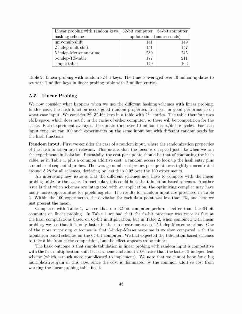
Linear probing with random keys 32-bit computer 64-bit computer

hashing scheme update time (nanoseconds)

univ-mult-shift 141 1492-indep-mult-shift 151 1575-indep-Mersenne-prime 289 2455-indep-TZ-table 177 211simple-table 149 166

Table 2: Linear probing with random 32-bit keys. The time is averaged over 10 million updates toset with 1 million keys in linear probing table with 2 million entries.

A.5 Linear Probing

We now consider what happens when we use the different hashing schemes with linear probing.In this case, the hash function needs good random properties are need for good performance onworst-case input. We consider 220 32-bit keys in a table with 221 entries. The table therefore uses8MB space, which does not fit in the cache of either computer, so there will be competition for thecache. Each experiment averaged the update time over 10 million insert/delete cycles. For eachinput type, we ran 100 such experiments on the same input but with different random seeds forthe hash functions.

Random input. First we consider the case of a random input, where the randomization propertiesof the hash function are irrelevant. This means that the focus is on speed just like when we ranthe experiments in isolation. Essentially, the cost per update should be that of computing the hashvalue, as in Table 1, plus a common additive cost: a random access to look up the hash entry plusa number of sequential probes. The average number of probes per update was tightly concentratedaround 3.28 for all schemes, deviating by less than 0.02 over the 100 experiments.

An interesting new issue is that the different schemes now have to compete with the linearprobing table for the cache. In particular, this could hurt the tabulation based schemes. Anotherissue is that when schemes are integrated with an application, the optimizing compiler may havemany more opportunities for pipelining etc. The results for random input are presented in Table2. Within the 100 experiments, the deviation for each data point was less than 1%, and here wejust present the mean.

Compared with Table 1, we see that our 32-bit computer performs better than the 64-bitcomputer on linear probing. In Table 1 we had that the 64-bit processor was twice as fast atthe hash computations based on 64-bit multiplication, but in Table 2, when combined with linearprobing, we see that it is only faster in the most extreme case of 5-indep-Mersenne-prime. Oneof the more surprising outcomes is that 5-indep-Mersenne-prime is so slow compared with thetabulation based schemes on the 64-bit computer. We had expected the tabulation based schemesto take a hit from cache competition, but the effect appears to be minor.

The basic outcome is that simple tabulation in linear probing with random input is competitivewith the fast multiplication-shift based scheme and about 20% faster than the fastest 5-independentscheme (which is much more complicated to implement). We note that we cannot hope for a bigmultiplicative gain in this case, since the cost is dominated by the common additive cost fromworking the linear probing table itself.

43

Structured input. We now consider the case where the input keys are structured in the sense ofbeing drawn in random order from a dense interval: a commonly occurring case in practice whichis known to cause unreliable performance for most simple hashing schemes [PPR09, PT10, TZ09].The results are shown in Figure 2. For each hashing scheme, we present the average number ofprobes for each of the 100 experiments as a cumulative distribution function. We see that simpletabulation and the 5-independent schemes remain tightly concentrated while the multiplication-shift schemes have significant variance, as observed also in [TZ09]. This behavior is repeated in thetimings on the two computers, but shifted due to difference in speed for the hash computations.

0

0.1

0.2

0.3

0.4

0.5

0.6

0.7

0.8

0.9

1

0 5 10 15 20

cum

ulat

ive

frac

tion

average probes per insert/delete

simple-tableuniv-mult-shift

2-indep-mult-shift5-indep-TZ-table

5-indep-Mersenne-prime

(a) Probe

0

0.1

0.2

0.3

0.4

0.5

0.6

0.7

0.8

0.9

1

0 100 200 300 400 500 600 700

cum

ulat

ive

frac

tion

average time per insert+delete cycle (nanoseconds)

simple-tableuniv-mult-shift

2-indep-mult-shift5-indep-TZ-table

5-indep-Mersenne-prime

(b) Time 32-bit computer

0

0.1

0.2

0.3

0.4

0.5

0.6

0.7

0.8

0.9

1

0 100 200 300 400 500 600 700

cum

ulat

ive

frac

tion

average time per insert+delete cycle (nanoseconds)

simple-tableuniv-mult-shift

2-indep-mult-shift5-indep-TZ-table

5-indep-Mersenne-prime

(c) Time 64-bit computer

Figure 2: Keys from dense interval. The multiplication-shift schemes sometimes use far moreprobes, which also shows in much longer running times.

Thus, among simple fast hashing schemes, simple tabulation stands out in not failing on a denseinterval. Of course, it might be that simple tabulation had a different worst-case input. A plausibleguess is that the worst instance of simple tabulation is the hypercube, which minimizes the amountof random table entries used. In our case, for 220 keys, we experimented with the set [32]4, i.e., weonly use 32 values for each of the 4 characters. The results for the number of probes are presentedin Figure 3.

Thus, simple tabulation remains extremely robust and tightly concentrated, but once again the

44

0

0.1

0.2

0.3

0.4

0.5

0.6

0.7

0.8

0.9

1

0 2 4 6 8 10cu

mul

ativ

e fr

actio

n

average probes per insert/delete

simple-tableuniv-mult-shift

2-indep-mult-shift5-indep-TZ-table

5-indep-Mersenne-prime

Figure 3: Keys from hyper cube.

multiplication-shift schemes fail (this time more often but less badly). The theoretical explanationfrom [PT10] is that multiplication-shift fails on arithmetic sequences, and in the hypercube we havemany different but shorter arithmetic sequences. It should be said that although it cannot be seenin the plots, the structured inputs did lead to more deviation in probes for simple tabulation: thedeviation from 3.28 over 100 independent runs grew from below 0.5% with random input to almost1% with any of the structured input.

Obviously, no experiment can confirm that simple tabulation is robust for all possible inputs.Our theoretical analysis implies strong concentration, e.g., in the sense of constant variance, yet thehidden constants are large. Our experiments suggest that the true constants are very reasonable.

Cuckoo hashing. Our results show that the failure probability in constructing a cuckoo hashingtable is O(n−1/3). A pertinent question is whether the constants hidden by the O-notation are toohigh from a practical point of view. Experiments cannot conclusively prove that this constant isalways small, since we do not know the worst instance. However, as for linear probing, a plausibleguess that the instance eliciting the worst behavior is a hypercube: S = Ac, for A ⊂ Σ. We made105 independent runs with the following input instances:

32-bit keys: Tabulation uses c = 4 characters. We set A = [32], giving 324 = 220 keys in S. Theempirical success probability was 99.4%.

64-bit keys: Tabulation uses c = 8 characters. We set A = 8, giving 88 = 224 keys in S. Theempirical success probability was 97.1%.

These experiments justify the belief that our scheme is effective in practice.It has already been shown conclusively that weaker multiplication schemes do not perform

well. Dietzfelbinger and Schellbach [DS09] show analytically that, when S is chosen uniformly atrandom from the universe [n12/11] or smaller, cuckoo hashing with 2-independent multiplicativehashing fails with probability 1− o(1). This is borne out in the experiments of [DS09], which givefailure probability close to 1 for random sets that are dense in the universe. On the other hand,the more complicated tabulation hashing of Thorup and Zhang [TZ04] will perform at least as wellas simple tabulation (that algorithm is a superset of simple tabulation).

A notable competitor to simple tabulation is a tailor-made tabulation hash function analyzed byDietzfelbinger and Woelfel [DW03]. This function uses two arrays of size r and four d-independenthash functions to obtain failure probability n/rd/2.

45

Let us analyze the parameters needed in a practical implementation. If we want the same spaceas in simple tabulation, we can set r = 210 (this is larger than Σ = 256, because fewer tables areneeded). For a nontrivial failure probability with sets of 220 keys, this would require 6-independence.In principle, the tabulation-based scheme of [TZ04] can support 6-independence with 5c− 4 tables(and lookups). This scheme has not been implemented yet, but based on combinatorial complexityis expected to be at least twice as slow as the 5-independent scheme tested in Table 1 (i.e. 4-8 timesslower than simple tabulation). Alternatively, we can compute four 6-independent hash functionsusing two polynomials of degree 5 on 64-bit values (e.g. modulo 261 − 1). Based on Table 1, thiswould be two orders of magnitude slower than simple tabulation. With any of the alternatives, thetailor-made scheme is much more complicated to implement.

B Chernoff Bounds with Fixed Means

We will here formally establish that the standard Chernoff bounds hold if when each variable havea fixed mean even if the of the variables are not independent. Below shall use the notation that ifwe have variables x1, x2, ..., then x<i = xjj<i. In particular,

∑x<i =

∑j<i xj .

Proposition 32. Consider n possibly dependent random variables X1, X2, . . . , Xn ∈ [0, 1]. Supposefor each i that E[Xi] = µi is fixed no matter the values of X1, ..., Xi−1, that is, for any valuesx1, ..., xi−1, E[Xi|X<i = x<i] = µi. Let X =

∑iXi and µ = E[X] =

∑i µi. Then for any δ > 0,

the bounds are:

Pr[X ≥ (1 + δ)µ] ≤(

eδ

(1 + δ)(1+δ)

)µPr[X ≤ (1− δ)µ] ≤

(e−δ

(1− δ)(1−δ)

)µProof. The proof is a simple generalization over the standard proof when the Xi are independent.We wish to bound the probability of X ≥ (1 + δ)µ. To do this we will prove that

E[(1 + δ)X ] ≤ eµ.

The proof will be by induction on n. Let

E[(1 + δ)X ] =∑x<n

⟨Pr[X<n = x<n]×E

[(1 + δ)X |X<n = x<n

]⟩=

∑x<n

⟨Pr[X<n = x<n]× (1 + δ)

∑x<n ×E

[(1 + δ)Xn |X<n = x<n

]⟩.

Now, for any random variable Y ∈ [0, 1], by convexity,

E[(1 + δ)Y

]≤ E[Y ](1 + δ) + 1−E[Y ] = 1 + δE[Y ] ≤ eδE[Y ]

Therefore, since E[Xn|X<n = x<n] = µn for any value x<n of X<n,

E[(1 + δ)Xn |X<n = x<n

]≤ eδµn .

46

Thus

E[(1 + δ)X ] =∑x<n

⟨Pr[X<n = x<n]× (1 + δ)

∑x<n ×E

[(1 + δ)Xn |X<n = x<n

]⟩.

≤∑x<n

⟨Pr[X<n = x<n]× (1 + δ)

∑x<n × eδµn

⟩= E

[(1 + δ)

∑X<n

]× eδµn

≤ eδ∑µ<n × eδµn = eδµ.

The last inequality followed by induction. Finally, by Markov’s inequality, we conclude that

Pr[X ≥ (1 + δ)µ] ≤E[(1 + δ)X

](1 + δ)(1+δ)µ

≤ eδµ

(1 + δ)(1+δ)µ=

(eδ

(1 + δ)(1+δ)

)µ.

The case X ≤ (1− δ)µ follows by a symmetric argument.

References

[BCL+10] Vladimir Braverman, Kai-Min Chung, Zhenming Liu, Michael Mitzenmacher, andRafail Ostrovsky. AMS without 4-wise independence on product domains. In Proc.27th Symposium on Theoretical Aspects of Computer Science (STACS), pages 119–130,2010.

[CK09] Jeffery S. Cohen and Daniel M. Kane. Bounds on the independence required for cuckoohashing. Manuscript, 2009.

[CW79] Larry Carter and Mark N. Wegman. Universal classes of hash functions. Journal ofComputer and System Sciences, 18(2):143–154, 1979. See also STOC’77.

[DHKP97] Martin Dietzfelbinger, Torben Hagerup, Jyrki Katajainen, and Martti Penttonen. Areliable randomized algorithm for the closest-pair problem. Journal of Algorithms,25(1):19–51, 1997.

[Die96] Martin Dietzfelbinger. Universal hashing and k-wise independent random variables viainteger arithmetic without primes. In Proc. 13th Symposium on Theoretical Aspects ofComputer Science (STACS), pages 569–580, 1996.

[DR09] Martin Dietzfelbinger and Michael Rink. Applications of a splitting trick. In Proc. 36thInternational Colloquium on Automata, Languages and Programming (ICALP), pages354–365, 2009.

[DS09] Martin Dietzfelbinger and Ulf Schellbach. On risks of using cuckoo hashing with simpleuniversal hash classes. In Proc. 20th ACM/SIAM Symposium on Discrete Algorithms(SODA), pages 795–804, 2009.

[DW03] Martin Dietzfelbinger and Philipp Woelfel. Almost random graphs with simple hashfunctions. In Proc. 25th ACM Symposium on Theory of Computing (STOC), pages629–638, 2003.

47

[Ger68] Leon Gerber. An extension of Bernoulli’s inequality. American Mathematical Monthly,75:875–876, 1968.

[Ind01] Piotr Indyk. A small approximately min-wise independent family of hash functions.Journal of Algorithms, 38(1):84–90, 2001. See also SODA’99.

[Knu63] Donald E. Knuth. Notes on open addressing. Unpublished memorandum. See http:

//citeseer.ist.psu.edu/knuth63notes.html, 1963.

[KR93] Howard J. Karloff and Prabhakar Raghavan. Randomized algorithms and pseudoran-dom numbers. Journal of the ACM, 40(3):454–476, 1993.

[MR95] Rajeev Motwani and Prabhakar Raghavan. Randomized algorithms. Cambridge Uni-versity Press, 1995.

[MV08] Michael Mitzenmacher and Salil P. Vadhan. Why simple hash functions work: exploit-ing the entropy in a data stream. In Proc. 19th ACM/SIAM Symposium on DiscreteAlgorithms (SODA), pages 746–755, 2008.

[PPR09] Anna Pagh, Rasmus Pagh, and Milan Ruzic. Linear probing with constant indepen-dence. SIAM Journal on Computing, 39(3):1107–1120, 2009. See also STOC’07.

[PT10] Mihai Patrascu and Mikkel Thorup. On the k-independence required by linear prob-ing and minwise independence. In Proc. 37th International Colloquium on Automata,Languages and Programming (ICALP), pages 715–726, 2010.

[Sie04] Alan Siegel. On universal classes of extremely random constant-time hash functions.SIAM Journal on Computing, 33(3):505–543, 2004. See also FOCS’89.

[SSS95] Jeanette P. Schmidt, Alan Siegel, and Aravind Srinivasan. Chernoff-Hoeffding boundsfor applications with limited independence. SIAM Journal on Discrete Mathematics,8(2):223–250, 1995. See also SODA’93.

[Tho00] Mikkel Thorup. Even strongly universal hashing is pretty fast. In Proc. 11thACM/SIAM Symposium on Discrete Algorithms (SODA), pages 496–497, 2000.

[Tho09] Mikkel Thorup. String hashing for linear probing. In Proc. 20th ACM/SIAM Symposiumon Discrete Algorithms (SODA), pages 655–664, 2009.

[TZ04] Mikkel Thorup and Yin Zhang. Tabulation based 4-universal hashing with applica-tions to second moment estimation. In Proc. 15th ACM/SIAM Symposium on DiscreteAlgorithms (SODA), pages 615–624, 2004.

[TZ09] Mikkel Thorup and Yin Zhang. Tabulation based 5-universal hashing and linear probing.In Proc. 12th Workshop on Algorithm Engineering and Experiments (ALENEX), 2009.

[WC81] Mark N. Wegman and Larry Carter. New classes and applications of hash functions.Journal of Computer and System Sciences, 22(3):265–279, 1981. See also FOCS’79.

48