Policy Research Working Paper 5081

The Power of ExportsWilliam Easterly

Ariell ReshefJulia Schwenkenberg

The World BankDevelopment Research GroupTrade and Integration Team &Latin America and the Caribbean RegionOffice of the Chief EconomistOctober 2009

WPS5081

Produced by the Research Support Team

Abstract

The Policy Research Working Paper Series disseminates the findings of work in progress to encourage the exchange of ideas about development issues. An objective of the series is to get the findings out quickly, even if the presentations are less than fully polished. The papers carry the names of the authors and should be cited accordingly. The findings, interpretations, and conclusions expressed in this paper are entirely those of the authors. They do not necessarily represent the views of the International Bank for Reconstruction and Development/World Bank and its affiliated organizations, or those of the Executive Directors of the World Bank or the governments they represent.

Policy Research Working Paper 5081

The authors systematically document remarkably high degrees of concentration in manufacturing exports for a sample of 151 countries over a range of 3,000 products. For every country manufacturing exports are dominated by a few "big hits" which account for most of the export value and where the "hit" includes both finding the right product and finding the right market. Higher export volumes are associated with higher degrees of concentration, after controlling for the number of destinations a country penetrates. This further highlights

This paper—a product of the Trade and Integration Team, Development Research Group and the Office of the Chief Economist, Latin America and the Caribbean Region—is part of a larger effort in both departments to study how the structure of trade affects development. Policy Research Working Papers are also posted on the Web at http://econ.worldbank.org. The author may be contacted at ar7kf@eservices.virginia.edu.

the importance of big hits. The distribution of exports closely follows a power law, especially in the upper tail. These findings do not support a "picking winners" policy for export development; the power law characterization implies that the chance of picking a winner diminishes exponentially with the degree of success. Moreover, given the size of the economy, developing countries are more exposed to demand shocks than rich ones, which further lowers the benefits from trying to pick winners.

The Power of Exports1

William Easterly Ariell Reshef Julia Schwenkenberg New York University New York University New York University and NBER

1 We thank Peter Debare, Jorg Stoye, Yijia Wang, Michael Waugh, participants at the World Bank invited session at LACEA 2008 and an anonymous referee for useful comments.

1 Introduction

How do countries succeed at economic development? Many descriptions of success stories

have stressed the important role of manufacturing exports as a vehicle for success. Indeed,

manufacturing exports per capita have a striking correlation with GDP per capita across

countries, see Figure 1. Causality could go either way in this association, or both variables

may re�ect other factors. The �gure does support a descriptive statement that success at

manufacturing exports and success at development are close to being the same thing. This

naturally warrants a close examination of the characteristics of success in export.

In this paper we show that manufacturing export success shows a remarkable degree

of specialization for virtually all countries. Manufacturing exports in each country are

dominated by a few �big hits�, which account for most of export value and where the

�hit� includes both �nding the right product and �nding the right market. Moreover, we

show that higher export volumes are associated with higher degrees of concentration, after

controlling for the number of destinations a country penetrates (i.e. absolute advantage and

size). This highlights the importance of big hits. In addition, we estimate that most of the

variation, and hence concentration, in export is driven by technological dispersion of the

exporting country, rather than demand shocks from the importing destinations. However,

given the size of the economy, developing countries are more exposed to demand shocks

than rich ones.

Hausmann and Rodrik (2006), in a seminal paper which helped inspire this one, had

previously pointed out the phenomenon of hyper-specialization, although only for a few

countries and products, and not including the destination component, in contrast to the

comprehensive scope of our work. We also make a very signi�cant addition to the Hausmann

and Rodrik �ndings, in that we characterize the probability of "big hits" as a function of

the size of the hit �by a power law.

We specify a �hit�as a product-by-destination export �ow. We chose this categorization

because some export products are shipped to several destinations, while the typical export

product is shipped to few destinations (with a mode of one). A few examples of big hits

and their relationship to concentration are in order. Out of 2985 possible manufacturing

products in our dataset and 217 possible destinations, Egypt gets 23 percent of its total

1

manufacturing exports from exporting one product ��Ceramic bathroom kitchen sanitary

items not porcelain��to one destination, Italy, capturing 94 percent of the Italian import

market for that product. Fiji gets 14 percent of its manufacturing exports from exporting

�Women�s, girl�s suits, of cotton, not knit� to the U.S., where it captures 42 percent of

U.S. imports of that product. The Philippines gets 10 percent of its manufacturing exports

from sending �Electronic integrated circuits/microassemblies, nes�to the U.S. (80 percent

of U.S. imports of that product). Nigeria earns 10 percent of its manufacturing exports from

shipping �Floating docks, special function vessels nes�to Norway, making up 84 percent of

Norwegian imports of that product.

Examining big hits that are exported almost exclusively to one destination for what

one would think would be fairly similar countries reveals a surprising diversity of products

and destinations. Why does Colombia export paint pigment to the U.S., but Costa Rica

exports data processing equipment, and Peru exports T-shirts? Why does Guatemala export

candles to the U.S., but El Salvador exports toilet and kitchen linens? Why does Honduras

export soap to El Salvador, while Nicaragua exports bathroom porcelain to Costa Rica?

Why does Cote d�Ivoire export perfume to Ghana, while Ghana exports plastic tables and

kitchen ware to Togo? Why does Uganda export electro-diagnostic apparatus to India,

while Malawi exports small motorcycle engines to Japan?

The remarkable specialization across products and destinations shows up in high con-

centration ratios. The top 1 percent of product-destination pairs account for an average of

52 percent of manufacturing export value for 151 countries on which we have data.1

The di¤erence between successful and unsuccessful exporters is found not just in the

degree of specialization, but also in the scale of the �big hits.�For example, a signi�cant part

of South Korea�s greater success than Tanzania as a manufacturing exporter is exempli�ed

by South Korea earning $13 billion from its top 3 manufacturing exports, while Tanzania

earned only $4 million from its top 3.

The probability of �nding a big hit ex ante decreases exponentially with the magnitude

of the hit. We show that the upper part of the distribution of export value across products

1At this point we do not analyze specialization (concentration) along the time dimension. One attemptto do so is Imbs and Wacziarg (2003). However, they address specialization in total production, not ex-ports, and, hence, do not analyze the destination dimension, which we believe captures additional productdi¤erentiation.

2

(de�ned both by destination and by six-digit industry classi�cations) is close to following a

power law.2 On average across our sample, the value of the 10th ranked product-destination

export category is only one-tenth of the top ranked product-destination export category.3

The value of the top ranked product-destination export category is on average 770 times

(median 34 times) larger than the 100th ranked product-destination export category. In

this paper we will estimate just how much the entire distribution of export values within

each country is explained by a power law, and will place it in the context of a trade model

with demand and productivity shocks.4

Realizing that export success is driven by a few big hits changes our understanding of

�success� and poses challenges for economic policy. Power laws may arise because many

conditions have to be satis�ed for a �big hit,�and hence the probability of success is given by

multiplying the probability of each condition being satis�ed times each other (if probabilities

are independent). Source country s�s success at exporting product p to destination country

d depends on industry-speci�c and country-speci�c productivity factors in country s, the

transport and relational connections between s and d in sector p, and the strength of

destination country d�s demand for product p from country s. All of these components

are subject to shocks in country-industry technology, �rms, country policy, input sectors,

shipping costs and technologies, trading relationships, brand reputation, tastes, competitors,

importing countries, etc.

The policy discussion about making such success more likely tends to be sharply polar-

ized. Hausmann and Rodrik argue that a �rm in country s that �rst succeeds at exporting

product p (they do not examine the destination dimension) is making a discovery that such

a product export is pro�table, which then has an externality to other �rms who can imitate

success. They argue therefore that such a discovery process should receive a public subsidy,

2Pareto distributions follow a so-called "power law", in which the probability of observing a particularvalue decreases exponentially with the size of that value. The distributions of word frequencies (Zipf�s law),sizes of cities, citations of scienti�c papers, web hits, copies of books sold, earthquakes, forest �res, solar�ares, moon craters and personal wealth all appear to follow power laws; see Newman (2005). See also Table1 in Andriani and McKelvey (2005) for more examples. Describing concentrated distributions in economicshas a long tradition, starting with Pareto (1896). Sutton (1997) provides a survey of the literature on thesize distribution of �rms starting with the observation of proportional growth by Gibrat (1931) (Gibrat�slaw).

3The corresponding median is lower �one fourth �because of the skewness of this number in our sample.4Luttmer (2007) constructs a general equilibrium model with �rm entry and exit that yields a power law

in �rm size. He combines a preference and a technology shock multiplicatively to obtain a variable he refersto as the �rm�s total factor productivity.

3

which may imply a conscious government industrial policy.

Our analysis raises a new issue. In addition to the possible knowledge externality to

a successful export, there is also a knowledge problem about the discovery itself. Who is

more likely to discover the successful product-destination category �the public or private

sector? We show that success (in both the product and destination dimensions) closely

follows a power law. Hence, ex ante picking a winning export category (or discoverer)

would be very hard indeed. A traditional argument for private entrepreneurship against

the government "picking winners" is that private entrepreneurship is a decentralized search

process characterized by many independent trials by agents who have many di¤erent kinds

of speci�c knowledge about sectors, markets, and technologies. This a priori seems more

likely to �nd a "big hit" than a process relying on centralized knowledge of the state.

However plausible these arguments may be, in the end it is an empirical question which

approaches work. We hope to stimulate this debate in this paper, but do not believe that

we can resolve it de�nitively.

A complementary point to ours is made by Besedes and Prusa (2008). They �nd that

most new trade relationships fail within 2 years and that the hazard rate of such failure

is higher for developing countries.5 Nevertheless, developing countries have the highest

increase in trade relationships: there seems to be a lot of attempts in discovery as it is.

However, entry (the extensive margin) does not account for much growth in trade. Together

with our stress on the importance and di¢ culty of discovering big hits (at a higher level of

disaggregation), this implies that Hausmann and Rodrik�s point might be misplaced.

Although addressing the Hausmann-Rodrik argument is our main goal, our work is

related to a few other recent papers. The observation that trade is concentrated has not been

lost on economists. Bernard, Jensen, Redding, and Schott (2007) document concentration

across U.S. exporting �rms, while Eaton, Eslava, Kugler, and Tybout (2007) �nd that

Colombian exports are dominated by a small number of very large (and stable) exporters.

Arkolakis and Muendler (2009) make a similar point for Brazilian and Chilean exporting

�rms and �nd that the distribution is approximately Pareto.

In contrast to these and other contributions, we document concentration and Pareto-like

distributions for many more countries (151); we do so at the product-destination level; and

5Their sample is 1975-2003 and relates to bilateral 4-digit SITC relationships.

4

we try to assess how much of this concentration is driven by technological dispersion versus

demand. Eaton, Kortum, and Kramarz (2008) also relate trade patterns to productivity and

demand shocks. But while they dissect trading patterns only for French �rms, regardless

of which products each �rm exports (there could be more than one product per �rm), we

analyze trade at the product level for many countries.6

In the next section we document concentration and distributions of exports for 151

countries in the product-destination dimension and perform preliminary analysis. In sec-

tion 3 we estimate the contribution of technology versus demand to the distribution and

concentration of exports. Section 4 concludes.

2 Empirical Facts

Our main data source is the UN Comtrade database. The U.N. classi�es exported commodi-

ties and manufactured products by source and destination at the six-digit level (roughly

5000 categories). We use the 1992 Harmonized System classi�cation (HS1992) for the year

2000, to maximize the available bilateral trade pairs. Using a less disaggregated classi�ca-

tion might have lead to better coverage of countries (say, 4-digit SITC), but would miss the

extreme concentration within �nely de�ned products.7

We restrict our sample to manufactured categories, i.e. we drop from the sample all

agriculture and commodities exports. Our focus on manufactured products stems from our

interest on exports that are not dependent on country-speci�c natural endowments, and

could potentially be produced everywhere in the world. We basically exclude products that

rely directly on natural resources. Natural resources create strong comparative advantage

for extracables and agricultural products. Therefore, a priori, focusing on manufacturing

also reduces the degree of concentration, especially for developing countries.

Some importers in the original dataset did not correspond to well-de�ned destinations,

so we dropped those destinations from the analysis.8 Eventually, our sample contains 151

exporters, 2984 export categories, which may be shipped to at most 217 destinations (im-

porters).

6The distribution of exports across products is similar to what they �nd for French �rms.7An analysis of the distribution of product-destination export �ows at the 4-digit SITC level reveals

similar patterns, but lower levels of concentration, as one might expect.8For example, �Antarctica�, �Areas, nes�, �Special Categories�, etc.

5

2.1 Concentration of exports

Our �rst observation is that exports are highly concentrated. That is, for each country a few

successful products and destination markets account for a disproportionately large share of

export value. We initially examine manufactured products, while ignoring the destination

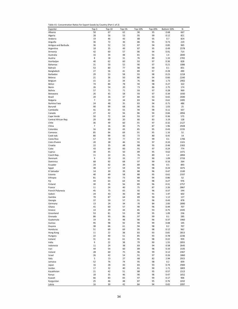
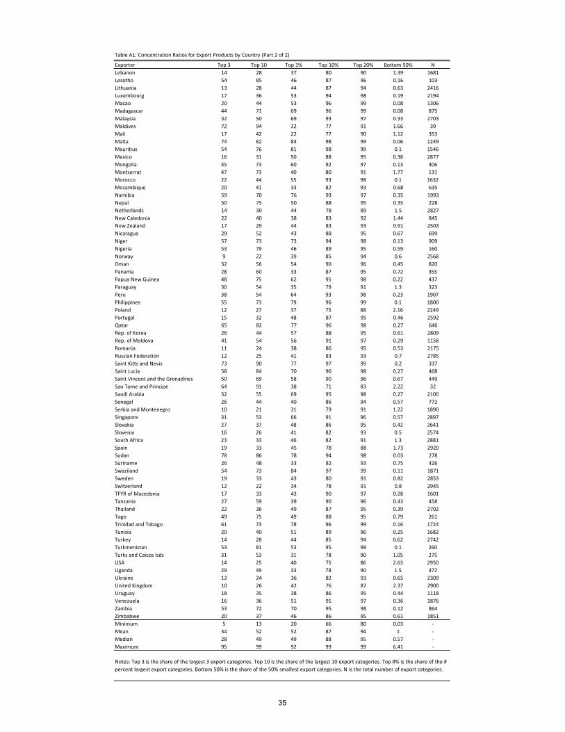
market dimension (we will incorporate the destinations shortly). Table 1 shows that the

median export share of the top 1%, 10% and 20% within nonzero export products for a

country is 49%, 86% and 94%, respectively.9 In fact, for the median country, the top 3

products account for 28% of exports, and the top 10 products account for a staggering 52%.

The median share for the bottom 50% of exported products is a mere 0.57%. This implies

a high degree of concentration indeed.10

One issue that complicates the interpretation of the concentration ratios is that countries

also di¤er a lot in how many export products they export at all (i.e. product exports with

nonzero entries for each country) �from a minimum of 10 to a maximum of 2950, with a

median of 1035. We will examine the role of number of products in the next section.

Another striking fact is just how few destination markets each product penetrates. Fig-

ure 2 shows the average across all 151 exporters of the share of export value accounted for

by products that have the number of destinations shown on the X-axis. The largest shares

go to products that are exported to only one destination, the next largest share goes to

products that are exported to only two destinations, and then it falls o¤ to a long tail. This

observation led to our decision to treat the product-destination pair as the unit of analysis

for the bulk of our analysis.

We now incorporate the destination dimension. In all the analysis that follows, we stick

to one unit of account: the product-destination export �ow. The same observation about

concentration at the product level holds for product-destination trade �ows, i.e. when each

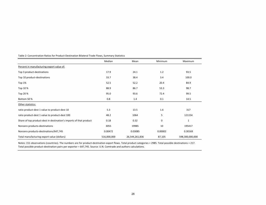
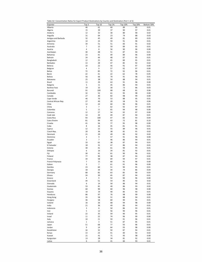
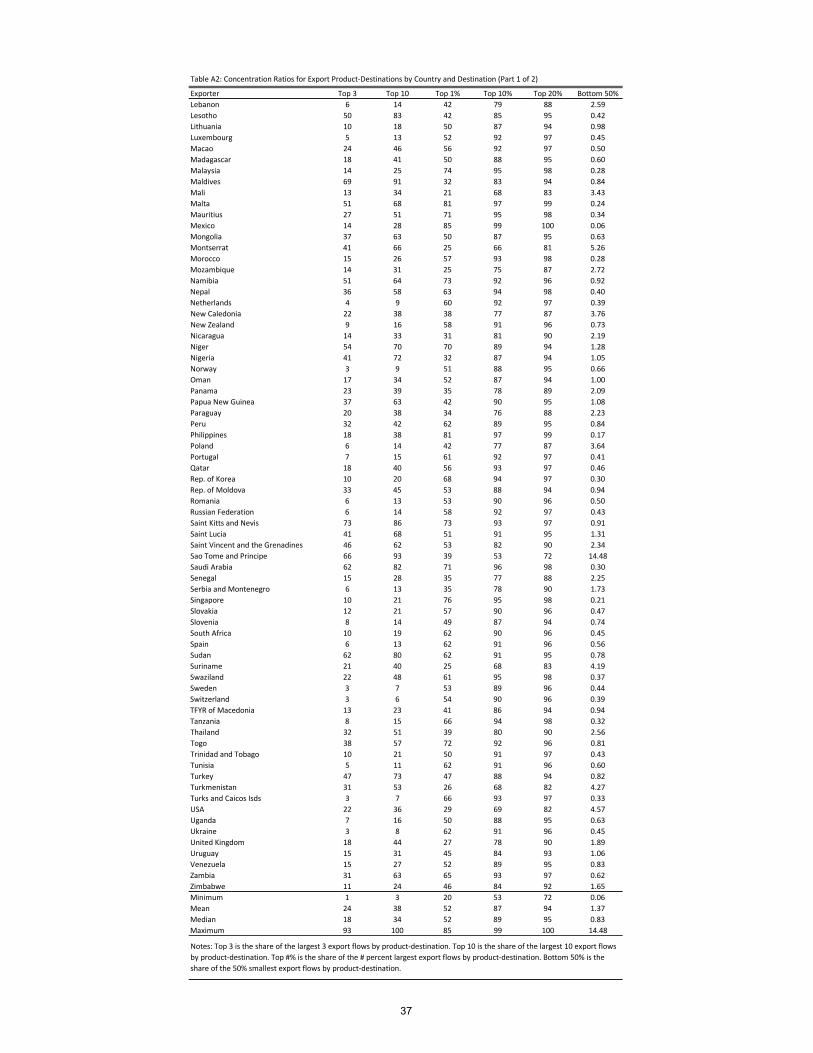
observation is an export of a particular product to a particular destination. Table 2 shows

that for the median exporter the top 1% of product-destination pairs account for 52.5% of

total export value! The top 10% account for 89% and the bottom 50% for only 0.8%.11

Once again, the number of nonzero entries in the product-destination matrix varies enor-

9Our basis for comparisons are always nonzero export �ows for each country separately. In calculatingpercentages we never compare to potential export products that are exported by all countries (2984 in total).10Table A1 in the appendix reports these shares for all 151 countries in our sample.11Table A2 in the appendix shows these numbers for all countries.

6

mously across countries, and is always far below the potential number implied by exporting

all products to all destinations. The median number of nonzero product-destination entries

per exporter is 3,055, going from a minimum of 10 to a maximum of 195,417. The median

number of nonzero entries is less than half of one percent of the potential number. Baldwin

and Harrigan (2007) have previously made the observation that many potential product-

destination �ows are absent and relate the incidence of zeros to distance and importer size.

Here we show that this is another important dimension of variation in the degree of suc-

cess of exports. In the next section we systematically relate this to concentration and the

prevalence of big hits.

2.2 Correlates of concentration

Our main focus is on the distribution of value across product-destination export �ows.

However, we want to �rst place the statistics above in context. To do so, we provide a brief

descriptive analysis of export patterns and concentration ratios. We start by illustrating

the very strong (log-linear) association between the number of nonzero product-destination

export �ows and the value of total manufacturing exports, as can be seen in Figure 3. One

way to succeed at exporting is to export more products to more places. This is a result of

absolute advantage, which allows penetrating more markets with more products.

Larger economies export more products to more destinations by virtue of sheer size and

diversity, and richer countries might have a better chance to penetrate more markets due

to better technology. This relationship between the number of product-destination export

�ows, size and income is well captured by the following regression, which we �t to data on

135 countries

log (number of nonzero export �ows) = �12:73(0:084)

+ 0:64(0:043)

�log (GDP)+ 0:65(0:084)

�log (GDP per capita) ;

where robust standard errors are reported in parentheses and R2 = 0:8.12 Poorer and

smaller economies indeed penetrate less markets with less products.

However, in terms of explaining export success, this is not the entire story, as Figure 4

shows. Even after controlling for size (GDP) and income (GDP per capita) the association

between export success and the number of nonzero product-destination export �ows remains

12We could obtain GDP data for only 135 countries in our sample.

7

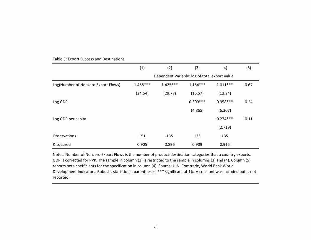
strong. In addition, Table 3 shows that the number of nonzero export �ows is the most

important factor: the beta coe¢ cient is three times larger and six times larger than those of

GDP and GDP per capita, respectively. We take this feature into account in our model. We

show how favorable productivity or demand shocks are necessary to overcome a threshold to

realize a non-zero entry (for either product or destination). Therefore, countries that exhibit

higher productivity levels also get to draw from a more favorable productivity distribution

and penetrate more destinations with more products.

We now return to describe concentration of exports across products and destinations.

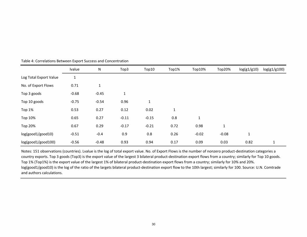
Table 4 shows the bivariate correlations between all the concentration statistics given

above. We see that the �top x�and �top x percent�concentration ratios are not measuring

the same thing; they are sometimes actually negatively related to each other. The problem is

that neither statistic is invariant to the number of nonzero product-destination �ows, which

varies a lot across countries, as we have seen. For mechanical reasons, a larger number of

nonzero product-destinations drives down the share of the �Top 3�or �Top 10�, but drives

up the share of the �Top 1 percent� or �Top 10 percent� (exactly the same e¤ect on the

concentration ratios is true for total manufacturing export value).

It is not clear whether we can construct an ideal concentration ratio when the number

of nonzero product-destinations varies so much. Our main results below don�t rely on

concentration ratios; instead, we characterize the entire shape of the distribution of nonzero

entries. The statistics on ratios of the top product-destination to the 10th ranked or 100th

ranked are closely related to the shares of the top 3 or top 10, and are related to the other

variables in the same way.

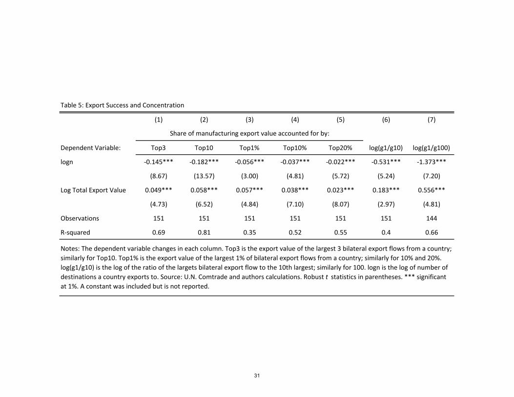
Finally, Table 5 examines the partial correlations between the concentration ratios and

the number of nonzero product-destinations export �ows and total manufacturing export

value (both in logs). The interesting result is that controlling for the number of nonzero

product-destination export �ows, total value is always positively associated with concentra-

tion (with both the top x and top x percent measures). It seems that the most successful

exporters by total value also have the highest concentration ratios for top x products or top

x percent of product-destination exports, conditional on the number of nonzero product-

destination export �ows they have. Given the level of total export value, a larger number

of product-destinations is associated with lower concentration. This makes sense, because

8

the same amount of export value must be distributed across more product-destinations.

We take this into account in our estimation below, in which we allow destination-speci�c

demand shocks.

The di¤erent e¤ects on concentration of the number of nonzero product-destination

export �ows versus total export value can be related to absolute and comparative advantage.

Countries that export a large number of products to many destinations exhibit absolute

advantage, or higher productivity, on average. For a given exporter facing all possible

destinations with entry �xed costs, a higher average productivity will allow it to penetrate

more destinations and export more products. But given the number of destinations an

exporting country penetrates, higher values come from productivity draws that are high

relative to the rest, which increases concentration. In our estimation procedure below we

will take this into account.

2.3 The distribution of exports: mixed lognormal-power law

A country�s most successful products account for the bulk of its total export value and

therefore the distribution of export values appears to be highly right-skewed. A candidate

distribution to describe this distribution would be the Pareto distribution which, as detailed

above, is used to explain a variety of highly skewed phenomena.

The Pareto distribution would imply a straight line on a log-log scale of export rank

and export value. We plot these rank graphs for all countries but observe that we have a

straight line only in the tails of the distributions as illustrated in Figure 5 for a selection of

countries.13 Eaton, Kortum, and Kramarz (2008) document similar rank graphs for French

�rms. Here we show that the shape holds for practically every country in our dataset.

These graphs indicate that the whole distribution does not �t the Pareto. But this is not

unusual in economic applications of the Pareto distribution; the same holds for income, �rm

size and city size.14 In all cases, a log normal distribution explains well the bottom of the

distribution, whereas the Pareto distribution �ts well the upper tail.

13U.S. (an established industrialized OECD economy), Ghana (a poor African country), Argentina (amiddle-income South American country), South Korea (a newly industrialized country, new to the OECD),China (the fast-growing giant) and Estonia (a small open transition economy). The data is by productcategory by destination and is demeaned by destination to control for the e¤ects of gravity and tradebarriers.14For example, see Eeckhout (2004).

9

We simulated a mixed Pareto-log normal random variable and a log-normal random

variable, and plotted their respective rank graphs in Figure 6. The simulated mixed Pareto-

log-normal random variable remarkably resembles our empirical distributions in Figure 5.

A visual comparison of the two simulated random variables in Figure 6 indicates that the

empirical graphs are �too straight�to �t the log normal. In other words, the distribution

of �success� across exports is so skewed that not even the highly skewed log normal can

be used to characterize it; it seems to require some combination of the log normal �which

is necessary at the least for the lower ranked product-destinations � and the power law

(Pareto) �which is required for the top ranked product-destinations. The simulated mixed

Pareto-log normal distribution seems to provide a better �t.

To formally reject lognormality of the data we performed two di¤erent normality tests on

log export values: the Kolmogorov-Smirno¤ test and a Normality test based on D�Agostino,

Belanger, and D�Agostino (1990). Normality is rejected in 85% with the former and in 93%

of the cases using the latter test. We conclude that the data cannot be described by a

log-normal alone.

In what follows we construct a simple demand-supply framework that yields a distrib-

ution of export values which is determined by log normal demand shocks and Pareto pro-

ductivity dispersion. Our innovation is to derive the lognormal-Pareto mixture distribution

for export values and determine the relative role the power law part plays.15

3 Technology versus Demand

In this section we raise the following question: How much of the variation in export values

is driven by technological dispersion in the source country versus demand shocks from

destination countries? Our interpretation of demand is broad, and includes true taste

shocks, �nding a good match and successful marketing. Answering this question can advise

policy on the types of tools that might �and those that might not �be relevant for promoting

trade.

Suppose that demand shocks are more important. This would imply that the stress

on �nding one�s comparative advantage is misplaced, because other forces determine trade

15Arkolakis (2008) develops a model with market penetration that takes into account marketing costs andmatches the distribution of exports better than a simple Pareto or log normal can.

10

�ows. An implication is that penetrating markets is more about marketing and �nding a

good match than high productivity. On the other hand, if technological dispersion is more

important, and if it follows a power law, then it would be very hard to predict big hits,

because the probability of predicting diminishes exponentially with the size of the hit (this

is the de�nition of a power law).

To this end we lay out a demand-supply framework which is similar to the backbone

of many modern trade models. This framework will allow us to estimate a parameter that

governs the distribution of technological dispersion and a parameter that governs demand

shocks. We examine empirically which accounts for a larger share of the variation in the

data, country by country. Our results indicate that productivity explains a larger percent

of variation in exports than demand shocks, and that this share is larger for less developed

countries.

In order not to burden the reader with familiar structure we present only the necessary

minimum of our framework and relegate the rest to the appendix.

3.1 Revenue and selection equations

Each destination country n is represented by one consumer, whose preferences over products

are represented by a CES aggregator. Products are indexed both by the product�s "name"

j and by source i.16 Optimal price taking behavior gives rise to the familiar CES demand

schedule

xn (i; j) = �n (i; j)

�pn (i; j)

pn

��� Ynpn

;

where �n (i; j) is a preference shock, pn (i; j) is the price to serve product j from source i

in destination n, pn and Yn are the price level and income in country n, respectively.17 As

usual, � > 1 is assumed, which is the same in all countries. It is also assumed that �n (i; j)

is independent of xn (i; j).

In source country i, producer j may export to any destination country n, including

domestic sales (n = i). Technology is linear in labor inputs. For a particular destination n,

16This follows the organization of the data in Comtrade and it implies product di¤erentiation at the good-source level. So widgets from Kenya are di¤erentiated from widgets from Costa Rica, even if they are bothcalled "widgets" in the data. This is essentially an Armington assumption.17See the appendix for a more complete description.

11

it chooses pn (i; j) to maximize pro�ts

�i (n; j) = pn (i; j)xn (i; j)� cn (i; j)xn (i; j)�Kn (i)

subject to the demand schedule. cn (i; j) is the producer�s (constant) marginal cost, which

is given by

cn (i; j) =w(i)

zn (i; j);

where w(i) are wages in country i and zn (i; j) is labor productivity. Kn (i) > 0 is a �xed

setup cost for business in i to penetrate the nmarket18. The implicit assumption here is that

there is just one such producer of product j in source country i that exports to destination

n, and there are no multiple-destination exporters. Thus, it is possible to produce slightly

di¤erent products per market.19 There are no other trade frictions.

Optimal pricing is a �xed markup over marginal cost. Thus, revenue for producer j in

source country i selling in destination n is given by

ri (n; j) = �n (i; j)

��

� � 1w(i)

zn (i; j)

�1��p��1n Yn :

Taking logs we get the following expression

ln ri (n; j) = �r0 � �wi + �pyn + ln�n (i; j) + (� � 1) ln zn (i; j) ; (1)

where �r0 = (1� �) ln ���1 , �

wi = (� � 1) lnw(i) , �pyn = (� � 1) ln pn + lnYn .

Equation (1) describes observed revenue, but does not take into account the fact that

overall pro�ts need to be non-negative, if we observe revenue at all. The selection equation

is

�i (n; j) = ri (n; j)� cn (i; j)xn (i; j)�Kn (i) � 0:

Using the previous results, optimal pricing yields

�n (i; j) � zn (i; j)��1 � �� (� � 1)1��Kn (i)

Yn

�w(i)

pn

���1:

This expression means that the demand shock and productivity must overcome a threshold.

18These capture making connections with potential buyers, adjusting the good to comply with localregulations, shipping costs, bribes at the border, etc�.19The data is aggregated over all producers anyway, so one can think that this represents a di¤erent mix

of producers.

12

The threshold is increasing in the size of the �xed cost for entry relative to the size of the

destination market (Kn (i) =Yn) and increasing in the real wage in the source country in

terms of the destination country (w(i)=pn). Taking logs and rearranging yields

ln�n (i; j) + (� � 1) ln zn (i; j) � �s0 + �wi � �pyn + �kin; (2)

where �s0 = ln��� (� � 1)1��

�, �kin = lnKn (i) and �

wi and �

pyn were de�ned above.

3.2 Empirical speci�cation

We would like to estimate the relative contribution of zn (i; j) versus �n (i; j) to the variation

of export revenues. To this end we will make some distributional assumptions that will

enable us to write down a likelihood function for export revenue. We will then maximize it

in order to retrieve the distribution parameters of the underlying productivity and demand

shocks. Using this information, we will be able to decompose the variance.

We assume that �n (i; j) is distributed log-normal such that ln�n (i; j) is distributed

normal with zero mean and variance v2.20 We do not index v2 by destination n, which

re�ects our assumption that in percent terms demand shocks should not be di¤erent across

countries. We assume that zn (i; j) in source country i is distributed Pareto,

Z � Fi (z) = 1��mi

z

�ai;

where z > mi > 0 and ai > 0. Note that mi varies by source country.21 It is assumed that

� and z are independent.

Equations (1) and (2) can then be written as

rinj = �r0 � �wi + �pyn + �inj + "inj (3)

and

�inj + "inj � �s0 + �wi � �pyn + �kin: (4)

where �inj = ln�n (i; j) is distributed normal for each destination with zero mean and

20Eaton, Kortum, and Kramarz (2008) also include lognormal demand shocks in their analysis of French�rms exporting behavior.21Helpman, Melitz, and Yeaple (2004) also assume a Pareto distribution for productivity, but do not let

it change by source country.

13

variance v2; and "inj = (� � 1) ln zn (i; j) is distributed conditional exponential

Fi(") = 1�maii e

� ai��1 ";

where we condition on " � (� � 1) ln(mi).22 De�ne

�i =ai� � 1

as the exponential parameter for ". So "inj is distributed exponential with conditional mean

(� � 1) ln(mi) + 1=�i.

Note that naively estimating (3) by least squares is not feasible. This is so because the

mean of "inj is not zero in general, so the intercept �wi is not separately identi�ed. However,

using maximum likelihood will allow us to overcome this issue.

By applying the Convolution Theorem (see appendix), we can characterize the distrib-

ution of �inj = �inj + "inj . Dropping the subscripts to ease notation, it turns out that the

p.d.f. of � is given by

f(�) = � exp

��2v2

2� ��

��

�� � �v2v

�; (5)

where � is the normal CDF. In (5) we assumed that mi = 1 for all i. This assumption

is innocuous because it does not a¤ect the estimates of v and �� we get the right ones

regardless. In the appendix we present the distribution of � for a general m, discuss iden-

ti�cation issues in detail and prove this last claim.23 Loosely speaking, this follows from

the characteristics of the underlying distributions: m is just a location parameter, while v

and � determine the shape of the distribution. We know that for the Pareto distribution,

the shape parameter a remains the same for any truncation from below. Similarly, for the

exponential distribution the shape parameter � is the same for any truncation from below.

As long as in all source countries some �rms draw productivities lower than the selection

cuto¤ and do not enter, assuming mi = 1 does not matter. This amounts to saying that

mi = 1 is low enough to ensure this.

Thus one can rewrite the revenue equation (3) and the selection equation (4) in terms

22Notice that (� � 1) ln(mi) can be positive or negative, but since mi > 0 and � > 1, (� � 1) ln(mi) isbounded away from �1. This is not a standard exponential random variable, in the sense that " can beless than zero, but all the properties of the exponential distribution are preserved.23We thank Yijia Wang for useful discussions of this matter.

14

of �.

3.3 Maximum likelihood estimation

We can rewrite the revenue equation to get an expression for �inj

�inj = rinj � �r0 + �wi � �pyn (6)

and then use it in the selection equation to get

rinj � �r0 + �s0 + �kin � trin;

where trin is the cuto¤ for observed revenue. Rearranging the expression for trin and plugging

it into the selection equation yields

�inj � trin � �r0 + �wi � �pyn : (7)

Of course, this follows directly from (6), if we replace rinj with its minimum value. Even-

tually, we have a modi�ed pair of equations for revenue (6) and selection (7) in terms of

�inj .

We estimate the model separately for each source country. Therefore, to ease notation

we drop the index i of the source country. For a given source country equations (6) and (7)

can be collapsed into the following representation

�nj = rnj � �n

and

�nj � trn � �n;

where �n = �r0 � �w + �pyn . In principle, we could plug all �n coe¢ cients straight into the

likelihood function, but estimating all �n dummy variables is not feasible, because they are

not identi�ed. This follows from the fact that �nj has a non-zero mean. Luckily, we are not

interested in these estimates. Therefore, we take the following route.

For each destination let

b0n =

Pj rkjI (k = n)jPj I (k = n)

2j

=1P

j I (k = n)j

Xj

rnj; (8)

15

which is just the average export value per destination, and is the OLS estimator from a

regression of export values on a set of destination-speci�c constants and a zero-mean error

term. The estimator b0n is a biased estimator of �n, but we know that the bias is equal to

1=�, i.e. E(b0n) = �n + 1=�. We take advantage of this in a two-step estimation procedure

in the following way.

� Step 1: Calculate b0n as shown above in (8).

� Step 2: De�ne

e�nj � rnj � b0n +

1b�etrn � trn � b0n +

1b�as our corrected � and truncation values, and maximize the following likelihood

L(bv; b�) = �nj f(e�nj)1� F (etrn) ;

with respect to b� and bv. Note that etrn = trn�b0n+1=b�, so that ftrng are also parametersto be estimated. In principle, we could also maximize the likelihood with respect to

ftrng. However, a consistent estimator of trn is

btrn = minjfrnjg :

We use btrn to replace trn in the estimation procedure, which simpli�es the estimationand is very robust.

In order to make sure that our procedure works, we performed Monte Carlo simulations

and backed out the original parameters successfully. The initial values for the maximum

likelihood numerical optimizer were chosen as empirical moments from the data. For each

source country the initial value for � was chosen as the average trade �ow, demeaned by

destination. The initial value for v was chosen as the standard deviation from that same

data. Changing the initial values for the search within a reasonable range did not a¤ect the

results.

16

3.4 Estimation results and variance decomposition

Figure 7 plots the estimated � parameters by country against log GDP per capita. Almost

all estimates of � fall within 0.5 and 1.24 Recall our interpretation for � = a= (� � 1). This

means that the technology distribution has remarkably similar Pareto coe¢ cients across

income levels, assuming elasticities of demand are also similar. Typical estimates of � in

similar settings are well above 2, in the range of 5-12 . This would place the estimate of

the Pareto coe¢ cient, a, above 2, which is reassuring, because it restricts the primitive

distribution of productivity in the model to have �nite �rst and second moments.

However, this would not imply that the level of the distributions of technology are the

same in all countries. As discussed in the end of section 3.2, we do not estimate the mi

parameters, which govern the actual level of productivity. Higher mi makes it more likely to

penetrate any given destination market. Countries that penetrate more destinations must

have higher mi. Nevertheless, the shape of the productivity distribution across countries is

similar.

We want to decompose the variance of � into variance due to the normal demand shocks

�, and the exponential technology component, ". We need to perform the variance de-

composition under the condition that the selection equation holds. For a given cuto¤ of a

speci�c destination n, we have

V (�j� � t (n)) = V (� + "j� � t (n)) = V (�j� � t (n)) + V ("j� � t (n)) ;

where t (n) varies over destinations and captures the fact that the cuto¤ changes by desti-

nation. The covariance term is zero due to the assumed independence of � and ". Closed

form solutions for the last two variance expressions are very complicated to derive, so we

simulate these expressions instead.25 The simulation procedure is described in the appen-

dix. A complication arises from the fact that the cuto¤, t, varies by destination n. In order

to address this issue, we decompose each conditional variance according to the variance

version of The Law of Iterated Expectations as follows

V (Xj� � t (n)) = Vn [E (Xj� � t (n))] + En [V (Xj� � t (n))] ; (9)

24Table A3 in the appendix presents all the estimates for �. The countries with extremely high estimatesof � are Burundi (2.9) and Benin (2), both of which have few observations.25We thanks Jorg Stoye for suggesting this.

17

where X represents either � or ". We report the percent contribution to the variance of �

of � and ":

p� = 100�V (�j� � t (n))V (�j� � t (n)) and p" = 100�

V ("j� � t (n))V (�j� � t (n)) :

In doing so, we report two sets of results; once where we do not use weights in (9), and then

using the number of observations per destination as weights.

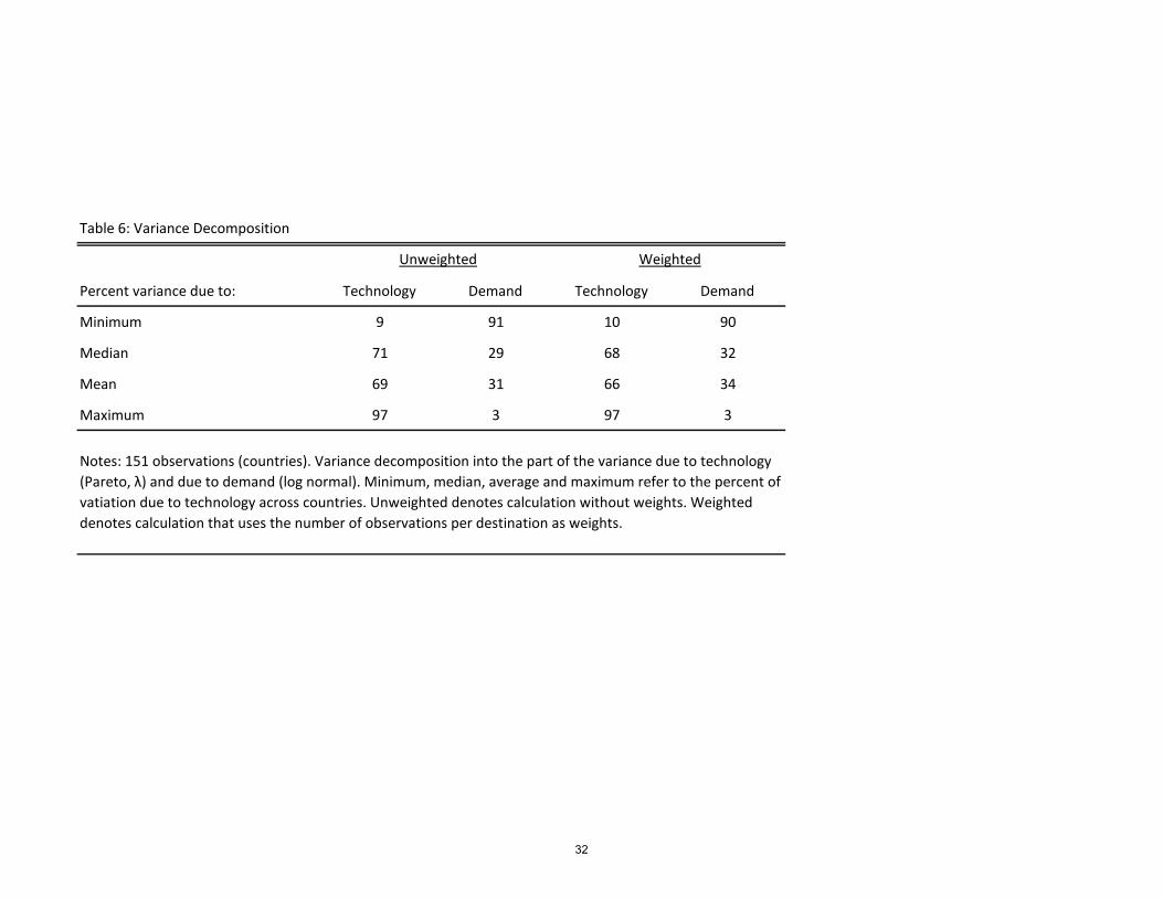
Table 6 presents our main result: on average 66% of the variance is due to the Pareto

part of the distribution.26 In Table 7 we report some correlates of p� in order to investigate

potential determinants of the percent of variance due to technology.

Figure 8 and column (1) of Table 7 indicate a negative relationship between the

percent of variance due to technology and the log of GDP. As we know from above, large

countries export to more destination and that should expose them to more demand shocks.

Indeed, there is also a negative relationship between the number of product-destination

export �ows and the percent of the variance due to technology, as can be seen in Figure 9

and in columns (2) and (3) of Table 7.

In column (4) of Table 7 we control for both the number of export �ows and for income

(GDP per capita). We �nd that the contribution of technology to the dispersion of export

is in fact higher in richer countries, controlling for the number of destinations they export

to.27 This is a point of interest. We know that richer countries do export more products

to more markets due to absolute advantage, which should expose them to more demand

shocks. However, it seems that developing countries are more exposed to demand shocks,

over and above their ability to penetrate more markets with more products.

4 Conclusion

In this paper we document the high degree of specialization in exports in a sample of 151

economies. Specialization is remarkably high in exporting manufactures, as in many other

areas in economics. The distribution is remarkably skewed. We �nd that very few "big

hits" account for a disproportionate share of export volumes and can also explain high

26Table A4 in the appendix shows the percent of the variance due to the Pareto component for allcountries.27Given the result in Figure 7, it is not surprising that we did not �nd a univariate correlation between

income and p�.

18

degrees of specialization. We also �nd that higher concentration (i.e., big hits) is positively

correlated with higher trade volumes, after controlling for the number of products that are

exported and destinations that are reached. Larger countries export more products to more

destinations and so do richer countries, where the latter is driven by absolute advantage.

Controlling for the number of product-destination export �ows, overall export volumes are

positively correlated with higher concentration, which are explained by big hits. This is

driven by comparative advantage.

We analyze the determinants of these big hits. We �nd that technology explains most

of the variation in export trade �ows, relative to demand shocks. This means that ex-

port success is mainly driven by technological dispersion, which also explains high levels

of specialization. Developing countries export less products to fewer destinations, which

helps explaining this. Exporting to more destinations exposes a country to more demand

shocks that are uncorrelated with technological dispersion. Therefore, as a country pene-

trates more markets with more products, demand shocks from those markets and for those

products account for a larger percent of variation �and hence concentration �in exports.

When we control for the number of markets and products we �nd that the relative con-

tribution of technology to the variation in exports is lower in developing countries. This

implies that developing countries are more exposed to demand shocks within the set of

product-destinations that they export.

Our analysis leads us to some important conclusions that are relevant for policies that

aim to promote trade. We �nd that a power law plays an important role in the distribu-

tion of export value across possible product-destination pairs. This makes the �erce debate

about the relative weights on the government and the market in �picking winners� even

more relevant than previously realized in the literature. A power law means that success-

fully picking a winner becomes less likely exponentially with the degree of success that

is predicted. Over and above this mechanism, the higher relative exposure of developing

countries to demand shocks, given their successful export �ows, implies an even smaller role

for picking winners.

The "picking winners" debate is about two things: probability of discovering a "winner"

and externalities from identifying the winner to other �rms. The traditional argument for

relying on free markets to decide what to produce is that they make possible a decentralized

19

search by myriads of entrepreneurs, and provide means for scaling up successful hits through

reinvestment of pro�ts and �nancing by capital markets. The probability of any one agent

�such as a government policymaker ��nding which product-destination combination will

be the big hit is very small. In fact, the track record of governments in picking winners

is not great, as Lee (1996) demonstrates for Korea.28 Hence, an alternative implication

� nearly the opposite of the Hausmann-Rodrik conclusion � of the hyper-specialization

phenomenon is that entrepreneurs and �nanciers should be as unhindered as possible from

any government intervention.

However, if there are externalities from the discovery of a "big hit" to other �rms who

can also export the same good-destination pair, then there is a market failure leading to too

little discovery e¤ort by any one entrepreneur. This leads to the traditional argument for

government intervention to subsidize "discovery", as Hausmann and Rodrik emphasized.

Perhaps one could try to get the best of both worlds by designing a blanket government

subsidy to all "discovery" e¤orts, while leaving the process of identifying the winners to

private entrepreneurs. How to design such a policy in practice, and whether the traditional

arguments fully apply to the stylized facts we have uncovered is far from de�nitive. Our

main contribution is to show that �nding winning hyper-specializations is even harder � and

yet the rewards to �nding these hyper-specializations are also even larger �than previously

thought.

28We are not saying that industrial policy in Korea did not contribute to its subsequent success. We onlypoint out that the "picking winners" part of that policy has not proven to be successful.

20

Appendix

A Demand structure

There are N countries. Let preferences in destination country n be given by

Un =

�Z�n (i; j)

1=� xn (i; j)��1� d (i; j)

� ���1

;

where xn (i; j) denotes product j from source country i and �n (i; j) are preference weights(shocks) associated with those products. As usual, � > 1 is assumed. We assume thatelasticities of substitution in demand, �, are the same in all countries. We assume that�n (i; j) are independent of xn (i; j).

Maximizing this utility function under the following budget constraintZpn (i; j)xn (i; j) d (i; j) � Yn

gives rise to demand

xn (i; j) = �n (i; j)

�pn (i; j)

pn

��� Ynpn

;

where Yn denotes nominal national income and pn is the perfect price index for destinationn,

pn =

�Z�n (i; j) pn (i; j)

1�� d (i; j)

� 11��

:

B The distribution of � = � + " for general m

Theorem 1 (Convolution Theorem29): if X and Y are independent continuous randomvariables with p.d.f.s fX(x) and fY (y), then the p.d.f. of Z = X + Y is

fZ(z) =

Z 1

�1fX(t)fY (z � t)dt :

De�ne the convoluted random variable � = � + ", where � is distributed normal withzero mean and variance v2 and " is distributed conditional exponential with exponent �and " � (� � 1) ln(m). Using the Convolution Theorem (see Casella and Berger (2002))

f�(�) =

Z 1

�1f"(t)

1

v�

�� � tv

�dt =

Z 1

(��1) lnmf"(t)

1

v�

�� � tv

�dt ;

where � is the Normal p.d.f. and we omit indexing by source and destination to easenotation. The second equality follows from the fact that " � (� � 1) ln(m), and f"(t) = 029Casella and Berger (2002).

21

when that condition is not met. Explicitly,

f�(�) =

Z 1

(��1) lnmma� exp f��tg 1p

2�v2exp

�� 1

2v2(� � t)2

�dt

= �ma

Z 1

0

1p2�v2

exp

���t� 1

2v2(�2 � 2�t+ t2)

�dt :

Focus on the exponent in the integrand:

��t� 1

2v2(�2 � 2�t+ t)2 = � 1

2v2�2�v2t+ �2 � 2�t+ t2

�= � 1

2v2��2 � 2

�� � �v2

�t+ t2

�and complete the square

= � 1

2v2

h�� � �v2 � t

�2+ 2�v2� �

��v2�2i

= � 1

2v2�t��� � �v2

��2+�2v2

2� ��

so that

f�(�) = �ma

Z 1

(��1) lnm

1p2�v2

exp

�� 1

2v2�t��� � �v2

��2+�2v2

2� ��

�dt

= �ma exp

��2v2

2� ��

�Z 1

(��1) lnm

1p2�v2

exp

�� 1

2v2�t��� � �v2

��2�dt :

Notice that the integrand is nothing but a p.d.f. of a normal random variable with mean�� � �v2

�and variance v2. So the integral itself is equal to

1�� (� � 1) lnm�

�� � �v2

�v

!= 1��

��� � �v

2 � (� � 1) lnmv

�= �

�� � �v2 � (� � 1) lnm

v

�and

f�(�) = �ma exp

��2v2

2� ��

��

�� � �v2 � (� � 1) lnm

v

�:

By setting m = 1 we get the result in the text.One can double-check this result by plugging the dummy variable in � rather than in

f" and deriving the same result from

f�(�) =

Z 1

�1

1

v�

�t

v

�f"(� � t)dt =

Z ��(��1) ln(m)

�1

1

v�

�t

v

�f"(� � t)dt :

where the second equality follows from the fact that � � t � (� � 1) ln(m) = 0 in this case,i.e., t � � � (� � 1) ln(m), and f"(� � t) = 0 when that condition is not met.

C Identi�cation issues: m and � are not identi�ed

As we know, � for a source country i has mean equal to (� � 1) ln(mi) + 1=�i. However,since we do not observe �, but only revenues, we cannot identify m, even if we hold � atsome value. The reason is that in order to get to � we need to deduct country �xed e¤ects,

22

which are not identi�ed separately from the mean of �. Moreover, holding m at any valuedoes not a¤ect the estimates of v and �.

To see this point formally, suppose that we actually used

e�nj = rnj � b0n + (e� � 1) ln em+ 1e�in the likelihood. This is the general expression for e� in the two-step procedure. Now plugthis into ln f (�) to get

ln f(e�) = ln�+ a lnm+�2v2

2� �e� + ln"� e� � �v2 � (� � 1) lnm

v

!#

= ln�+ a lnm+�2v2

2� �

�rnj � b

0n + (� � 1) lnm+

1

�

�

+ ln

24�0@�rnj � b

0n + (� � 1) lnm+ 1

�

�� �v2 � (� � 1) lnm

v

1A35= ln�+ a lnm+

�2v2

2� �

�rnj � b

0n

�� a

� � 1 (� � 1) lnm� 1

+ ln

"�

rnj � b

0n + 1=�� �v2v

!#

= ln�+�2v2

2� �

�rnj � b

0n

�� 1 + ln

"�

rnj � b

0n + 1=�

v� �v

!#:

As one can see, m and � drop out. Doing the same in lnF (e�) yields the same result. So mand � are completely absent from the likelihood function. This proves that in the estimationprocedure we get the same estimates of v and �� regardless of the values of m and �.

The two-step estimation procedure described above takes this into account by assuming aparticular location (m = 1) and identifying v and � solely from the shape of the distribution.Thus, the variance decomposition is correct regardless of the values of m and �.

D Simulating conditional variances

Here we describe the algorithm for simulating the conditional variances for each sourcecountry i. We start with a set of estimates of � and v for each source country, and cuto¤values t (n) for each destination country, per each source country.

1. Draw a large number D (we use D = 100; 000) of uniform (u) and standard normal(z) random variables and store them. Both vectors are (D � 1) and will be used forall countries and destinations.

2. Given estimates of � and v for source i, compute exponential productivity values, e,and normal demand shocks, d, as follows

e = � ln(1� u)=b�d = bv � z

23

and

e2 = e2

d2 = d2 ;

where it is understood that we apply the the square operator to each element sepa-rately. Thus, the vectors e, e2, d and d2 are all (D � 1).

3. Sum d and e to get the simulated theta

e� = d+ e :4. For each destination n, generate a (D � 1) indicator vector

I�e� � t (n)� :

5. Compute

E [Xj� � t] =EhX � I

�e� � t (n)�iEhI�e� � t (n)�i =

1DX

0I�e� � t (n)�

1D �

0I�e� � t (n)� ;

where � is just a (D � 1) vector of ones, and X can be either e , e2, d or d2. Thus,we get simulated values for E [�j� � t], E

��2j� � t

�, E ["j� � t], E

�"2j� � t

�. We use

these values to compute variances according to

V (Xj� � t (n)) = E�X2j� � t (n)

�+ [E (Xj� � t (n))]2 :

6. Repeat 4� 5 for each destination n, and store the results.

7. UseV (Xj� � t) = Vn [E (Xj� � t (n))] + En [V (Xj� � t (n))]

to compute the conditional variance of � and ", where the values inside brackets arecalculated in 4� 6 and the operators over n (Vn [�] and En [�]) use sample analogues.Calculate Vn [�] and En [�] in two ways: once without weights and then using thenumber of observations per destination for each exporter as weights.

Repeat 2� 7 for each source country.

24

References

Andriani, P., and B. McKelvey (2005): �Why Gaussian statistics are mostly wrong forstrategic organization,�Strategic Organization, 3(2), 219�228.

Arkolakis, K. (2008): �Market Penetration Costs and the New Consumers Margin inInternational Trade,�Yale Working Paper.

Arkolakis, K., and M.-A. Muendler (2009): �The Extensive Margin of ExportingGoods: A Firm-Level Analysis,�Yale Working Paper.

Baldwin, R., and J. Harrigan (2007): �Zeros, Quality and Space: Trade Theory andTrade Evidence,�NBER Working Paper 13214.

Bernard, A., B. Jensen, S. Redding, and P. Schott (2007): �Firms in InternationalTrade,�Journal of Economic Perspectives, 21(3), 105�130.

Besedes, T., and T. J. Prusa (2008): �The Role of Extensive and Intensive Margins andExport Growth,�Working Paper.

Casella, G., and R. L. Berger (2002): Statistical Inference, second edition.

D�Agostino, R. B., A. Belanger, and R. B. J. D�Agostino (1990): �A Suggestion forUsing Powerful and Informative Tests of Normality,�The American Statistician, 44(4),316�321.

Eaton, J., M. Eslava, M. Kugler, and J. Tybout (2007): �Export Dynamics inColombia: Firm-Level Evidence,�NBER Working Paper 13531.

Eaton, J., S. Kortum, and F. Kramarz (2008): �An Anatomy of International Trade:Evidence from French Firms,�Working Paper.

Eeckhout, J. (2004): �Gibrat�s Law for (all) Cities,�American Economic Review, 94(5),1429�1451.

Gibrat, R. (1931): Les ine ,tgalite ,ts e ,tconomiques; applications: aux ine ,tgalite ,ts desrichesses, a�la concentration des entreprises, aux populations des villes, aux statistiquesdes familles, etc., d�une loi nouvelle, la loi de l�e¤et proportionnel. Librairie du RecueilSirey, Paris.

Hausmann, R., and D. Rodrik (2006): �Doomed to Choose: Industrial Policy as Predica-ment,�Working Paper.

Helpman, E., M. Melitz, and S. Yeaple (2004): �Exports vs. FDI with HeterogeneousFirms,�American Economic Review, 94(1), 300�316.

Imbs, J., and R. Wacziarg (2003): �Stages of Diversi�cation,� American EconomicReview, 93(1), 63�86.

Lee, J.-W. (1996): �Government Interventions and Productivity Growth,� Journal ofEconomic Growth, 1(2), 391�414.

Luttmer, E. G. J. (2007): �Selection, Growth and the Size Distribution of Firms,�Quar-terly Journal of Economics, August, 1103�1144.

25

Newman, M. E. J. (2005): �Power Laws, Pareto Distributions and Zipf�s Law,�Contem-porary Physics, 46(5), 323�351.

Pareto, V. (1896): Cours d�Economie Politique. Droz, Geneva.

Sutton, J. (1997): �Gibrat�s Legacy,�Journal of Economic Literature, 35, 40�59.

26

Median Mean Minimum Maximum

Percent of the following in total manufacturing export revenues:

Top 3 products 28 34 5 96

Top 10 products 49 52 13 100

Top 1% 47 48 18 92

Top 10% 86 85 43 99

Top 20% 94 93 66 99

Bottom 50% 0.8 1.3 0.1 17.3

Other statistics:

Ratio of Top product value to 10th ranked product value 7.2 20.3 1.8 626.6

Ratio of Top product value to 100th ranked product value 104.8 1004.1 10.8 84478.2

Share of Top product in world import market for that product 0.018 0.066 0 0.698

Number of products exported (# of nonzero entries) 1035 1302 10 2950

Table 1: Concentration Ratios for Export Products by Country, Summary Statistics

Notes: 151 observations (countries). The numbers are for export vlaues by product, regardless of the unmber of export destinations. Source: U.N. Comtrade and authors calculations.

27

Median Mean Minimum Maximum

Percent in manufacturing export value of:

Top 3 product-destinations 17.9 24.1 1.2 93.5

Top 10 product-destinations 33.7 38.4 3.4 100.0

Top 1% 52.5 52.2 20.4 84.9

Top 10 % 88.9 86.7 53.3 98.7

Top 20 % 95.0 93.6 72.4 99.5

Bottom 50 % 0.8 1.4 0.1 14.5

Other statistics:

ratio product-dest 1 value to product-dest 10 5.3 13.5 1.6 317

ratio product-dest 1 value to product-dest 100 48.2 1064 5 121154

Share of top product-dest in destination's imports of that product 0.18 0.32 0 1

Nonzero products-destinations 3055 19985 10 195417

Nonzero products-destinations/647,745 0.00472 0.03085 0.00002 0.30169

Total manufacturing export value (dollars) 516,000,000 26,544,261,836 87,105 598,300,000,000

Table 2: Concentration Ratios for Product-Destination Bilateral Trade Flows, Summary Statistics

Notes: 151 observations (countries). The numbers are for product-destination export flows. Total product categories = 2985. Total possible destinations = 217. Total possible product-destination pairs per exporter = 647,745. Source: U.N. Comtrade and authors calculations.

28

(1) (2) (3) (4) (5)

Log(Number of Nonzero Export Flows) 1.458*** 1.425*** 1.164*** 1.011*** 0.67

(34.54) (29.77) (16.57) (12.24)

Log GDP 0.309*** 0.358*** 0.24

(4.865) (6.307)

Log GDP per capita 0.274*** 0.11

(2.719)

Observations 151 135 135 135

R-squared 0.905 0.896 0.909 0.915

Notes: Number of Nonzero Export Flows is the number of product-destination categories that a country exports. GDP is corrected for PPP. The sample in column (2) is restricted to the sample in columns (3) and (4). Column (5) reports beta coefficients for the specification in column (4). Source: U.N. Comtrade, World Bank World Development Indicators. Robust t statistics in parentheses. *** significant at 1%. A constant was included but is not reported.

Dependent Variable: log of total export value

Table 3: Export Success and Destinations

29

lvalue N Top3 Top10 Top1% Top10% Top20% log(g1/g10) log(g1/g100)

Log Total Export Value 1

No. of Export Flows 0.71 1

Top 3 goods -0.68 -0.45 1

Top 10 goods -0.75 -0.54 0.96 1

Top 1% 0.53 0.27 0.12 0.02 1

Top 10% 0.65 0.27 -0.11 -0.15 0.8 1

Top 20% 0.67 0.29 -0.17 -0.21 0.72 0.98 1

log(good1/good10) -0.51 -0.4 0.9 0.8 0.26 -0.02 -0.08 1

log(good1/good100) -0.56 -0.48 0.93 0.94 0.17 0.09 0.03 0.82 1

Table 4: Correlations Between Export Success and Concentration

Notes: 151 observations (countries). Lvalue is the log of total export value. No. of Export Flows is the number of nonzero product-destination categories a country exports. Top 3 goods (Top3) is the export value of the largest 3 bilateral product-destination export flows from a country; similarly for Top 10 goods. Top 1% (Top1%) is the export value of the largest 1% of bilateral product-destination export flows from a country; similarly for 10% and 20%. log(good1/good10) is the log of the ratio of the largets bilateral product-destination export flow to the 10th largest; similarly for 100. Source: U.N. Comtrade and authors calculations.

30

(1) (2) (3) (4) (5) (6) (7)

Dependent Variable: Top3 Top10 Top1% Top10% Top20% log(g1/g10) log(g1/g100)

logn -0.145*** -0.182*** -0.056*** -0.037*** -0.022*** -0.531*** -1.373***

(8.67) (13.57) (3.00) (4.81) (5.72) (5.24) (7.20)

Log Total Export Value 0.049*** 0.058*** 0.057*** 0.038*** 0.023*** 0.183*** 0.556***

(4.73) (6.52) (4.84) (7.10) (8.07) (2.97) (4.81)

Observations 151 151 151 151 151 151 144

R-squared 0.69 0.81 0.35 0.52 0.55 0.4 0.66

Notes: The dependent variable changes in each column. Top3 is the export value of the largest 3 bilateral export flows from a country; similarly for Top10. Top1% is the export value of the largest 1% of bilateral export flows from a country; similarly for 10% and 20%. log(g1/g10) is the log of the ratio of the largets bilateral export flow to the 10th largest; similarly for 100. logn is the log of number of destinations a country exports to. Source: U.N. Comtrade and authors calculations. Robust t statistics in parentheses. *** significant at 1%. A constant was included but is not reported.

Table 5: Export Success and Concentration

Share of manufacturing export value accounted for by:

31

Percent variance due to: Technology Demand Technology Demand

Minimum 9 91 10 90

Median 71 29 68 32

Mean 69 31 66 34

Maximum 97 3 97 3

Table 6: Variance Decomposition

Unweighted Weighted

Notes: 151 observations (countries). Variance decomposition into the part of the variance due to technology (Pareto, λ) and due to demand (log normal). Minimum, median, average and maximum refer to the percent of vatiation due to technology across countries. Unweighted denotes calculation without weights. Weighted denotes calculation that uses the number of observations per destination as weights.

32

(1) (2) (3) (4)

Log GDP -2.534***

(-4.055)

Log Export Flows -2.365*** -2.338** -3.756***

(-2.885) (-2.411) (-4.019)

Log GDP per capita 3.342***

(2.723)

Observations 135 151 135 135

R-squared 0.123 0.101 0.094 0.132

Table 7: Correlates of Variance Contribution of Technology

Notes: Export Flows is the number of product-destination categories that a country exports. GDP is corrected for PPP. The sample in column (3) is restricted to the sample in columns (1) and (4). Source: World Bank World Development Indicators and author calculations. Robust t statistics in parentheses. *** and ** significant at 1% and 5%, respectively. A constant was included but is not reported.

Dependent Variable: Percent Variance due to Technology

33

Exporter Top 3 Top 10 Top 1% Top 10% Top 20% Bottom 50% NAlbania 50 67 62 90 95 0.68 667Algeria 28 56 53 95 99 0.12 821Andorra 19 46 43 88 95 0.7 824Anguilla 36 72 36 86 95 0.73 219Antigua and Barbuda 36 52 52 87 94 0.85 965Argentina 18 35 49 87 95 0.49 2578Armenia 42 60 57 86 94 0.91 714Australia 16 34 48 81 91 1.4 2840Austria 8 18 31 76 89 1.33 2765Azerbaijan 40 62 60 93 97 0.36 828Bahamas 31 50 52 90 97 0.21 1086Bahrain 53 80 77 98 99 0.1 851Bangladesh 27 56 41 89 97 0.28 490Barbados 29 53 58 93 98 0.23 1218Belarus 21 36 50 86 94 0.66 2240Belgium 15 22 34 76 88 1.73 2902Belize 74 86 78 94 98 0.27 322Benin 26 54 20 73 86 2.75 174Bolivia 57 71 71 93 97 0.28 969Botswana 26 45 58 93 97 0.34 1930Brazil 20 34 47 84 93 0.65 2690Bulgaria 7 19 34 83 94 0.61 2495Burkina Faso 24 48 35 83 94 0.75 486Burundi 90 99 68 90 95 1.03 25Cambodia 41 65 55 94 98 0.11 507Canada 27 42 56 86 94 0.66 2856Cape Verde 50 72 64 93 97 0.36 575Central African Rep. 29 60 20 66 83 3.19 128Chile 36 49 60 91 97 0.32 2127China 7 16 30 75 87 1.96 2928Colombia 16 30 43 85 95 0.43 2235Comoros 85 94 69 91 95 1.16 52Cook Isds 80 99 43 72 80 6.41 14Costa Rica 57 70 77 97 99 0.1 1706Cote d'Ivoire 20 38 46 91 97 0.33 1321Croatia 22 35 48 88 95 0.46 2302Cuba 43 64 60 91 97 0.24 774Cyprus 30 45 50 89 95 0.62 1471Czech Rep. 11 22 35 76 89 1.4 2894Denmark 9 19 33 77 90 1.09 2733Dominica 68 92 68 97 99 0.16 264Ecuador 24 42 39 89 96 0.5 893Egypt 38 57 59 94 98 0.24 1075El Salvador 14 30 39 88 96 0.47 1530Estonia 40 49 58 88 95 0.61 2337Ethiopia 81 93 73 88 94 0.86 52Fiji 44 63 63 94 98 0.27 976Finland 30 45 56 89 96 0.31 2757France 11 24 40 75 87 2.26 2867French Polynesia 45 75 65 92 96 0.57 544Gabon 24 43 36 80 91 1.47 602Gambia 70 87 64 89 94 1.12 127Georgia 37 59 57 91 96 0.43 878Germany 13 24 34 70 84 2.83 2890Ghana 41 60 57 90 96 0.49 707Greece 14 29 44 85 93 0.75 2445Greenland 53 81 53 90 95 1.09 236Grenada 86 93 86 97 99 0.1 285Guatemala 19 35 48 90 96 0.37 1960Guinea 95 98 92 99 99 0.08 145Guyana 38 66 61 94 98 0.2 707Honduras 51 69 69 95 98 0.12 962Hong Kong 11 22 38 83 93 0.81 2813Hungary 22 40 51 85 93 0.78 2236Iceland 31 61 61 95 98 0.22 959India 9 22 38 79 90 1.55 2855Indonesia 11 24 38 83 94 0.58 2645Iran 44 54 60 89 96 0.33 1535Ireland 28 60 75 96 99 0.12 2467Israel 26 42 54 91 97 0.26 1860Italy 5 13 27 68 82 2.94 2915Jamaica 52 76 74 95 98 0.2 839Japan 16 28 43 83 93 0.74 2900Jordan 17 32 40 81 90 1.71 1803Kazakhstan 21 42 51 88 95 0.57 1513Kenya 18 35 46 90 96 0.47 1652Kuwait 66 83 83 97 99 0.17 906Kyrgyzstan 25 46 48 87 95 0.76 1032Latvia 16 30 42 84 94 0.65 2097

Table A1: Concentration Ratios for Export Goods by Country (Part 1 of 2)

34

Exporter Top 3 Top 10 Top 1% Top 10% Top 20% Bottom 50% NLebanon 14 28 37 80 90 1.39 1681Lesotho 54 85 46 87 96 0.16 103Lithuania 13 28 44 87 94 0.63 2416Luxembourg 17 36 53 94 98 0.19 2194Macao 20 44 53 96 99 0.08 1306Madagascar 44 71 69 96 99 0.08 875Malaysia 32 50 69 93 97 0.33 2703Maldives 72 94 32 77 91 1.66 39Mali 17 42 22 77 90 1.12 353Malta 74 82 84 98 99 0.06 1249Mauritius 54 76 81 98 99 0.1 1546Mexico 16 31 50 88 95 0.38 2877Mongolia 45 73 60 92 97 0.13 406Montserrat 47 73 40 80 91 1.77 131Morocco 22 44 55 93 98 0.1 1632Mozambique 20 41 33 82 93 0.68 635Namibia 59 70 76 93 97 0.35 1993Nepal 50 75 50 88 95 0.35 228Netherlands 14 30 44 78 89 1.5 2827New Caledonia 22 40 38 83 92 1.44 845New Zealand 17 29 44 83 93 0.91 2503Nicaragua 29 52 43 88 95 0.67 699Niger 57 73 73 94 98 0.13 909Nigeria 53 79 46 89 95 0.59 160Norway 9 22 39 85 94 0.6 2568Oman 32 56 54 90 96 0.45 820Panama 28 60 33 87 95 0.72 355Papua New Guinea 48 75 62 95 98 0.22 437Paraguay 30 54 35 79 91 1.3 323Peru 38 54 64 93 98 0.23 1907Philippines 55 73 79 96 99 0.1 1800Poland 12 27 37 75 88 2.16 2249Portugal 15 32 48 87 95 0.46 2592Qatar 65 82 77 96 98 0.27 646Rep. of Korea 26 44 57 88 95 0.61 2809Rep. of Moldova 41 54 56 91 97 0.29 1158Romania 11 24 38 86 95 0.53 2175Russian Federation 12 25 41 83 93 0.7 2785Saint Kitts and Nevis 73 90 77 97 99 0.2 337Saint Lucia 58 84 70 96 98 0.27 468Saint Vincent and the Grenadines 50 69 58 90 96 0.67 449Sao Tome and Principe 64 91 38 71 83 2.22 32Saudi Arabia 32 55 69 95 98 0.27 2100Senegal 26 44 40 86 94 0.57 772Serbia and Montenegro 10 21 31 79 91 1.22 1890Singapore 31 53 66 91 96 0.57 2897Slovakia 27 37 48 86 95 0.42 2641Slovenia 16 26 41 82 93 0.5 2574South Africa 23 33 46 82 91 1.3 2881Spain 19 33 45 78 88 1.73 2920Sudan 78 86 78 94 98 0.03 278Suriname 26 48 33 82 93 0.75 426Swaziland 54 73 84 97 99 0.11 1871Sweden 19 33 43 80 91 0.82 2853Switzerland 12 22 34 78 91 0.8 2945TFYR of Macedonia 17 33 43 90 97 0.28 1601Tanzania 27 59 39 90 96 0.43 458Thailand 22 36 49 87 95 0.39 2702Togo 49 75 49 88 95 0.79 261Trinidad and Tobago 61 73 78 96 99 0.16 1724Tunisia 20 40 51 89 96 0.25 1682Turkey 14 28 44 85 94 0.62 2742Turkmenistan 53 81 53 95 98 0.1 260Turks and Caicos Isds 31 53 31 78 90 1.05 275USA 14 25 40 75 86 2.63 2950Uganda 29 49 33 78 90 1.5 372Ukraine 12 24 36 82 93 0.65 2309United Kingdom 10 26 42 76 87 2.37 2900Uruguay 18 35 38 86 95 0.44 1118Venezuela 16 36 51 91 97 0.36 1876Zambia 53 72 70 95 98 0.12 864Zimbabwe 20 37 46 86 95 0.61 1851Minimum 5 13 20 66 80 0.03 -Mean 34 52 52 87 94 1 -Median 28 49 49 88 95 0.57 -Maximum 95 99 92 99 99 6.41 -

Table A1: Concentration Ratios for Export Products by Country (Part 2 of 2)

Notes: Top 3 is the share of the largest 3 export categories. Top 10 is the share of the largest 10 export categories. Top #% is the share of the # percent largest export categories. Bottom 50% is the share of the 50% smallest export categories. N is the total number of export categories.

35

Exporter Top 3 Top 10 Top 1% Top 10% Top 20% Bottom 50%Albania 46 61 60 89 95 0.01Algeria 15 39 37 90 97 0.01Andorra 12 32 30 80 90 0.02Anguilla 31 64 23 74 88 0.03Antigua and Barbuda 32 45 49 81 89 0.03Argentina 14 24 59 91 96 0.01Armenia 34 51 51 83 91 0.02Australia 7 15 59 89 95 0.01Austria 4 8 56 90 96 0.00Azerbaijan 30 48 51 87 94 0.01Bahamas 23 41 49 89 96 0.00Bahrain 24 44 48 87 95 0.01Bangladesh 12 25 45 89 95 0.01Barbados 13 28 47 85 92 0.02Belarus 10 22 56 91 97 0.00Belgium 4 9 57 92 97 0.00Belize 72 85 72 92 96 0.01Benin 22 41 22 62 78 0.05Bolivia 56 66 70 91 96 0.01Botswana 25 38 50 88 94 0.01Brazil 11 20 63 91 96 0.00Bulgaria 5 11 45 86 94 0.01Burkina Faso 19 33 30 73 86 0.03Burundi 91 100 68 68 81 0.06Cambodia 32 52 61 95 98 0.00Canada 27 40 82 98 99 0.00Cape Verde 46 70 53 88 95 0.01Central African Rep. 27 49 20 58 76 0.06Chile 12 24 60 90 96 0.01China 3 7 62 92 97 0.00Colombia 5 11 65 94 98 0.00Comoros 12 27 54 92 97 0.00Cook Isds 14 20 49 87 94 0.01Costa Rica 93 100 47 82 93 0.04Cote d'Ivoire 81 99 43 72 81 0.10Croatia 41 56 77 95 98 0.00Cuba 8 16 35 81 91 0.01Cyprus 12 21 55 89 96 0.01Czech Rep. 20 36 38 81 91 0.02Denmark 21 29 49 85 92 0.02Dominica 4 9 57 91 96 0.00Ecuador 3 7 46 86 94 0.01Egypt 33 61 38 87 94 0.01El Salvador 18 31 47 86 94 0.01Estonia 30 41 61 90 95 0.01Ethiopia 6 16 34 81 92 0.01Fiji 30 41 61 90 96 0.01Finland 77 90 38 87 94 0.02France 34 58 69 94 97 0.01French Polynesia 7 15 60 91 96 0.00Gabon 3 7 61 91 96 0.00Gambia 23 60 51 90 95 0.01Georgia 18 34 34 74 86 0.04Germany 68 82 63 85 90 0.03Ghana 24 39 45 87 94 0.01Greece 4 9 54 90 96 0.00Greenland 34 51 54 85 92 0.02Grenada 6 14 50 86 94 0.01Guatemala 53 81 40 86 93 0.02Guinea 60 90 60 96 98 0.00Guyana 10 19 40 85 93 0.01Honduras 86 97 76 98 99 0.00Hong Kong 35 58 51 88 94 0.01Hungary 36 58 60 90 95 0.01Iceland 16 26 68 94 98 0.00India 21 36 49 85 94 0.01Indonesia 3 8 50 86 93 0.01Iran 5 12 56 90 96 0.01Ireland 22 35 59 90 95 0.01Israel 11 22 74 96 99 0.00Italy 10 21 59 91 96 0.01Jamaica 1 3 51 87 95 0.01Japan 51 68 77 93 96 0.01Jordan 9 14 64 93 98 0.00Kazakhstan 16 32 50 87 94 0.01Kenya 13 23 41 83 92 0.02Kuwait 21 41 71 95 98 0.00Kyrgyzstan 13 28 34 81 92 0.02Latvia 6 15 41 84 93 0.01

Table A2: Concentration Ratios for Export Product-Destinations by Country and Destination (Part 1 of 2)

36

Exporter Top 3 Top 10 Top 1% Top 10% Top 20% Bottom 50%Lebanon 6 14 42 79 88 2.59Lesotho 50 83 42 85 95 0.42Lithuania 10 18 50 87 94 0.98Luxembourg 5 13 52 92 97 0.45Macao 24 46 56 92 97 0.50Madagascar 18 41 50 88 95 0.60Malaysia 14 25 74 95 98 0.28Maldives 69 91 32 83 94 0.84Mali 13 34 21 68 83 3.43Malta 51 68 81 97 99 0.24Mauritius 27 51 71 95 98 0.34Mexico 14 28 85 99 100 0.06Mongolia 37 63 50 87 95 0.63Montserrat 41 66 25 66 81 5.26Morocco 15 26 57 93 98 0.28Mozambique 14 31 25 75 87 2.72Namibia 51 64 73 92 96 0.92Nepal 36 58 63 94 98 0.40Netherlands 4 9 60 92 97 0.39New Caledonia 22 38 38 77 87 3.76New Zealand 9 16 58 91 96 0.73Nicaragua 14 33 31 81 90 2.19Niger 54 70 70 89 94 1.28Nigeria 41 72 32 87 94 1.05Norway 3 9 51 88 95 0.66Oman 17 34 52 87 94 1.00Panama 23 39 35 78 89 2.09Papua New Guinea 37 63 42 90 95 1.08Paraguay 20 38 34 76 88 2.23Peru 32 42 62 89 95 0.84Philippines 18 38 81 97 99 0.17Poland 6 14 42 77 87 3.64Portugal 7 15 61 92 97 0.41Qatar 18 40 56 93 97 0.46Rep. of Korea 10 20 68 94 97 0.30Rep. of Moldova 33 45 53 88 94 0.94Romania 6 13 53 90 96 0.50Russian Federation 6 14 58 92 97 0.43Saint Kitts and Nevis 73 86 73 93 97 0.91Saint Lucia 41 68 51 91 95 1.31Saint Vincent and the Grenadines 46 62 53 82 90 2.34Sao Tome and Principe 66 93 39 53 72 14.48Saudi Arabia 62 82 71 96 98 0.30Senegal 15 28 35 77 88 2.25Serbia and Montenegro 6 13 35 78 90 1.73Singapore 10 21 76 95 98 0.21Slovakia 12 21 57 90 96 0.47Slovenia 8 14 49 87 94 0.74South Africa 10 19 62 90 96 0.45Spain 6 13 62 91 96 0.56Sudan 62 80 62 91 95 0.78Suriname 21 40 25 68 83 4.19Swaziland 22 48 61 95 98 0.37Sweden 3 7 53 89 96 0.44Switzerland 3 6 54 90 96 0.39TFYR of Macedonia 13 23 41 86 94 0.94Tanzania 8 15 66 94 98 0.32Thailand 32 51 39 80 90 2.56Togo 38 57 72 92 96 0.81Trinidad and Tobago 10 21 50 91 97 0.43Tunisia 5 11 62 91 96 0.60Turkey 47 73 47 88 94 0.82Turkmenistan 31 53 26 68 82 4.27Turks and Caicos Isds 3 7 66 93 97 0.33USA 22 36 29 69 82 4.57Uganda 7 16 50 88 95 0.63Ukraine 3 8 62 91 96 0.45United Kingdom 18 44 27 78 90 1.89Uruguay 15 31 45 84 93 1.06Venezuela 15 27 52 89 95 0.83Zambia 31 63 65 93 97 0.62Zimbabwe 11 24 46 84 92 1.65Minimum 1 3 20 53 72 0.06Mean 24 38 52 87 94 1.37Median 18 34 52 89 95 0.83Maximum 93 100 85 99 100 14.48

Table A2: Concentration Ratios for Export Product-Destinations by Country and Destination (Part 1 of 2)

Notes: Top 3 is the share of the largest 3 export flows by product-destination. Top 10 is the share of the largest 10 export flows by product-destination. Top #% is the share of the # percent largest export flows by product-destination. Bottom 50% is the share of the 50% smallest export flows by product-destination.

37

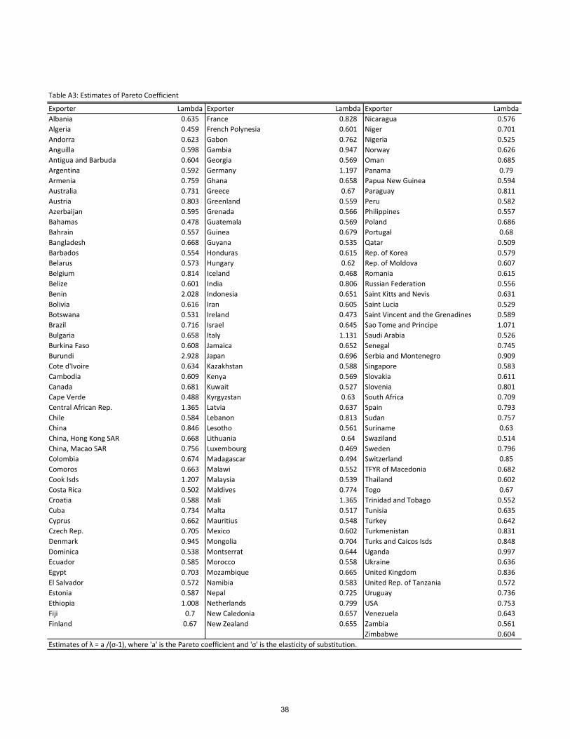
Exporter Lambda Exporter Lambda Exporter LambdaAlbania 0.635 France 0.828 Nicaragua 0.576Algeria 0.459 French Polynesia 0.601 Niger 0.701Andorra 0.623 Gabon 0.762 Nigeria 0.525Anguilla 0.598 Gambia 0.947 Norway 0.626Antigua and Barbuda 0.604 Georgia 0.569 Oman 0.685Argentina 0.592 Germany 1.197 Panama 0.79Armenia 0.759 Ghana 0.658 Papua New Guinea 0.594Australia 0.731 Greece 0.67 Paraguay 0.811Austria 0.803 Greenland 0.559 Peru 0.582Azerbaijan 0.595 Grenada 0.566 Philippines 0.557Bahamas 0.478 Guatemala 0.569 Poland 0.686Bahrain 0.557 Guinea 0.679 Portugal 0.68Bangladesh 0.668 Guyana 0.535 Qatar 0.509Barbados 0.554 Honduras 0.615 Rep. of Korea 0.579Belarus 0.573 Hungary 0.62 Rep. of Moldova 0.607Belgium 0.814 Iceland 0.468 Romania 0.615Belize 0.601 India 0.806 Russian Federation 0.556Benin 2.028 Indonesia 0.651 Saint Kitts and Nevis 0.631Bolivia 0.616 Iran 0.605 Saint Lucia 0.529Botswana 0.531 Ireland 0.473 Saint Vincent and the Grenadines 0.589Brazil 0.716 Israel 0.645 Sao Tome and Principe 1.071Bulgaria 0.658 Italy 1.131 Saudi Arabia 0.526Burkina Faso 0.608 Jamaica 0.652 Senegal 0.745Burundi 2.928 Japan 0.696 Serbia and Montenegro 0.909Cote d'Ivoire 0.634 Kazakhstan 0.588 Singapore 0.583Cambodia 0.609 Kenya 0.569 Slovakia 0.611Canada 0.681 Kuwait 0.527 Slovenia 0.801Cape Verde 0.488 Kyrgyzstan 0.63 South Africa 0.709Central African Rep. 1.365 Latvia 0.637 Spain 0.793Chile 0.584 Lebanon 0.813 Sudan 0.757China 0.846 Lesotho 0.561 Suriname 0.63China, Hong Kong SAR 0.668 Lithuania 0.64 Swaziland 0.514China, Macao SAR 0.756 Luxembourg 0.469 Sweden 0.796Colombia 0.674 Madagascar 0.494 Switzerland 0.85Comoros 0.663 Malawi 0.552 TFYR of Macedonia 0.682Cook Isds 1.207 Malaysia 0.539 Thailand 0.602Costa Rica 0.502 Maldives 0.774 Togo 0.67Croatia 0.588 Mali 1.365 Trinidad and Tobago 0.552Cuba 0.734 Malta 0.517 Tunisia 0.635Cyprus 0.662 Mauritius 0.548 Turkey 0.642Czech Rep. 0.705 Mexico 0.602 Turkmenistan 0.831Denmark 0.945 Mongolia 0.704 Turks and Caicos Isds 0.848Dominica 0.538 Montserrat 0.644 Uganda 0.997Ecuador 0.585 Morocco 0.558 Ukraine 0.636Egypt 0.703 Mozambique 0.665 United Kingdom 0.836El Salvador 0.572 Namibia 0.583 United Rep. of Tanzania 0.572Estonia 0.587 Nepal 0.725 Uruguay 0.736Ethiopia 1.008 Netherlands 0.799 USA 0.753Fiji 0.7 New Caledonia 0.657 Venezuela 0.643Finland 0.67 New Zealand 0.655 Zambia 0.561

Zimbabwe 0.604Estimates of λ = a /(σ-1), where 'a' is the Pareto coefficient and 'σ' is the elasticity of substitution.

Table A3: Estimates of Pareto Coefficient

38

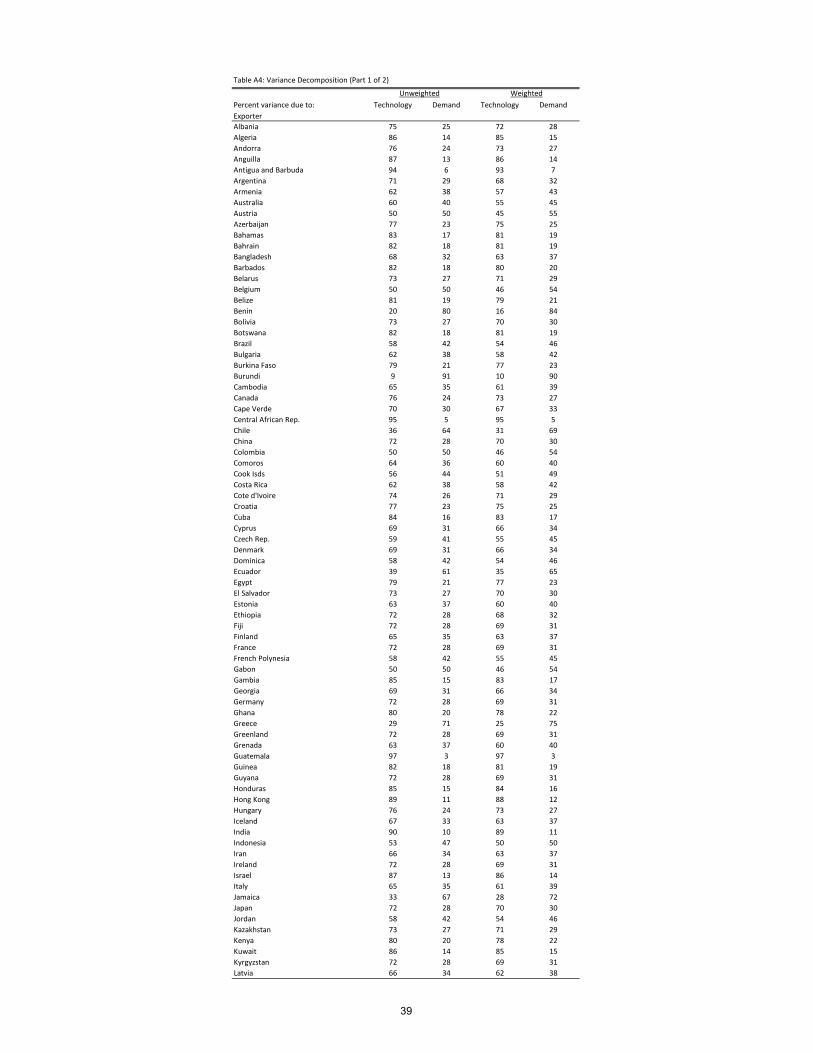
Percent variance due to: Technology Demand Technology DemandExporterAlbania 75 25 72 28Algeria 86 14 85 15Andorra 76 24 73 27Anguilla 87 13 86 14Antigua and Barbuda 94 6 93 7Argentina 71 29 68 32Armenia 62 38 57 43Australia 60 40 55 45Austria 50 50 45 55Azerbaijan 77 23 75 25Bahamas 83 17 81 19Bahrain 82 18 81 19Bangladesh 68 32 63 37Barbados 82 18 80 20Belarus 73 27 71 29Belgium 50 50 46 54Belize 81 19 79 21Benin 20 80 16 84Bolivia 73 27 70 30Botswana 82 18 81 19Brazil 58 42 54 46Bulgaria 62 38 58 42Burkina Faso 79 21 77 23Burundi 9 91 10 90Cambodia 65 35 61 39Canada 76 24 73 27Cape Verde 70 30 67 33Central African Rep. 95 5 95 5Chile 36 64 31 69China 72 28 70 30Colombia 50 50 46 54Comoros 64 36 60 40Cook Isds 56 44 51 49Costa Rica 62 38 58 42Cote d'Ivoire 74 26 71 29Croatia 77 23 75 25Cuba 84 16 83 17Cyprus 69 31 66 34Czech Rep. 59 41 55 45Denmark 69 31 66 34Dominica 58 42 54 46Ecuador 39 61 35 65Egypt 79 21 77 23El Salvador 73 27 70 30Estonia 63 37 60 40Ethiopia 72 28 68 32Fiji 72 28 69 31Finland 65 35 63 37France 72 28 69 31French Polynesia 58 42 55 45Gabon 50 50 46 54Gambia 85 15 83 17Georgia 69 31 66 34Germany 72 28 69 31Ghana 80 20 78 22Greece 29 71 25 75Greenland 72 28 69 31Grenada 63 37 60 40Guatemala 97 3 97 3Guinea 82 18 81 19Guyana 72 28 69 31Honduras 85 15 84 16Hong Kong 89 11 88 12Hungary 76 24 73 27Iceland 67 33 63 37India 90 10 89 11Indonesia 53 47 50 50Iran 66 34 63 37Ireland 72 28 69 31Israel 87 13 86 14Italy 65 35 61 39Jamaica 33 67 28 72Japan 72 28 70 30Jordan 58 42 54 46Kazakhstan 73 27 71 29Kenya 80 20 78 22Kuwait 86 14 85 15Kyrgyzstan 72 28 69 31Latvia 66 34 62 38

Unweighted Weighted

Table A4: Variance Decomposition (Part 1 of 2)

39

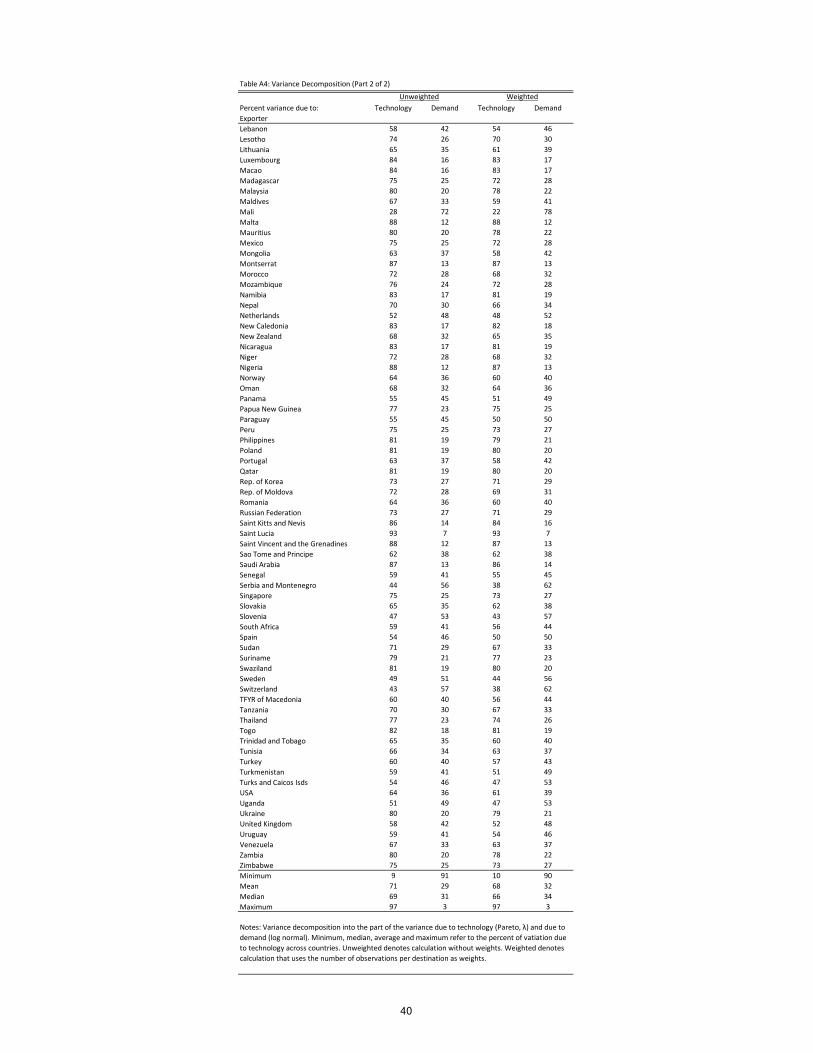
Percent variance due to: Technology Demand Technology DemandExporterLebanon 58 42 54 46Lesotho 74 26 70 30Lithuania 65 35 61 39Luxembourg 84 16 83 17Macao 84 16 83 17Madagascar 75 25 72 28Malaysia 80 20 78 22Maldives 67 33 59 41Mali 28 72 22 78Malta 88 12 88 12Mauritius 80 20 78 22Mexico 75 25 72 28Mongolia 63 37 58 42Montserrat 87 13 87 13Morocco 72 28 68 32Mozambique 76 24 72 28Namibia 83 17 81 19Nepal 70 30 66 34Netherlands 52 48 48 52New Caledonia 83 17 82 18New Zealand 68 32 65 35Nicaragua 83 17 81 19Niger 72 28 68 32Nigeria 88 12 87 13Norway 64 36 60 40Oman 68 32 64 36Panama 55 45 51 49Papua New Guinea 77 23 75 25Paraguay 55 45 50 50Peru 75 25 73 27Philippines 81 19 79 21Poland 81 19 80 20Portugal 63 37 58 42Qatar 81 19 80 20Rep. of Korea 73 27 71 29Rep. of Moldova 72 28 69 31Romania 64 36 60 40Russian Federation 73 27 71 29Saint Kitts and Nevis 86 14 84 16Saint Lucia 93 7 93 7Saint Vincent and the Grenadines 88 12 87 13Sao Tome and Principe 62 38 62 38Saudi Arabia 87 13 86 14Senegal 59 41 55 45Serbia and Montenegro 44 56 38 62Singapore 75 25 73 27Slovakia 65 35 62 38Slovenia 47 53 43 57South Africa 59 41 56 44Spain 54 46 50 50Sudan 71 29 67 33Suriname 79 21 77 23Swaziland 81 19 80 20Sweden 49 51 44 56Switzerland 43 57 38 62TFYR of Macedonia 60 40 56 44Tanzania 70 30 67 33Thailand 77 23 74 26Togo 82 18 81 19Trinidad and Tobago 65 35 60 40Tunisia 66 34 63 37Turkey 60 40 57 43Turkmenistan 59 41 51 49Turks and Caicos Isds 54 46 47 53USA 64 36 61 39Uganda 51 49 47 53Ukraine 80 20 79 21United Kingdom 58 42 52 48Uruguay 59 41 54 46Venezuela 67 33 63 37Zambia 80 20 78 22Zimbabwe 75 25 73 27Minimum 9 91 10 90Mean 71 29 68 32Median 69 31 66 34Maximum 97 3 97 3

Unweighted Weighted

Table A4: Variance Decomposition (Part 2 of 2)

Notes: Variance decomposition into the part of the variance due to technology (Pareto, λ) and due to demand (log normal). Minimum, median, average and maximum refer to the percent of vatiation due to technology across countries. Unweighted denotes calculation without weights. Weighted denotes calculation that uses the number of observations per destination as weights.

40

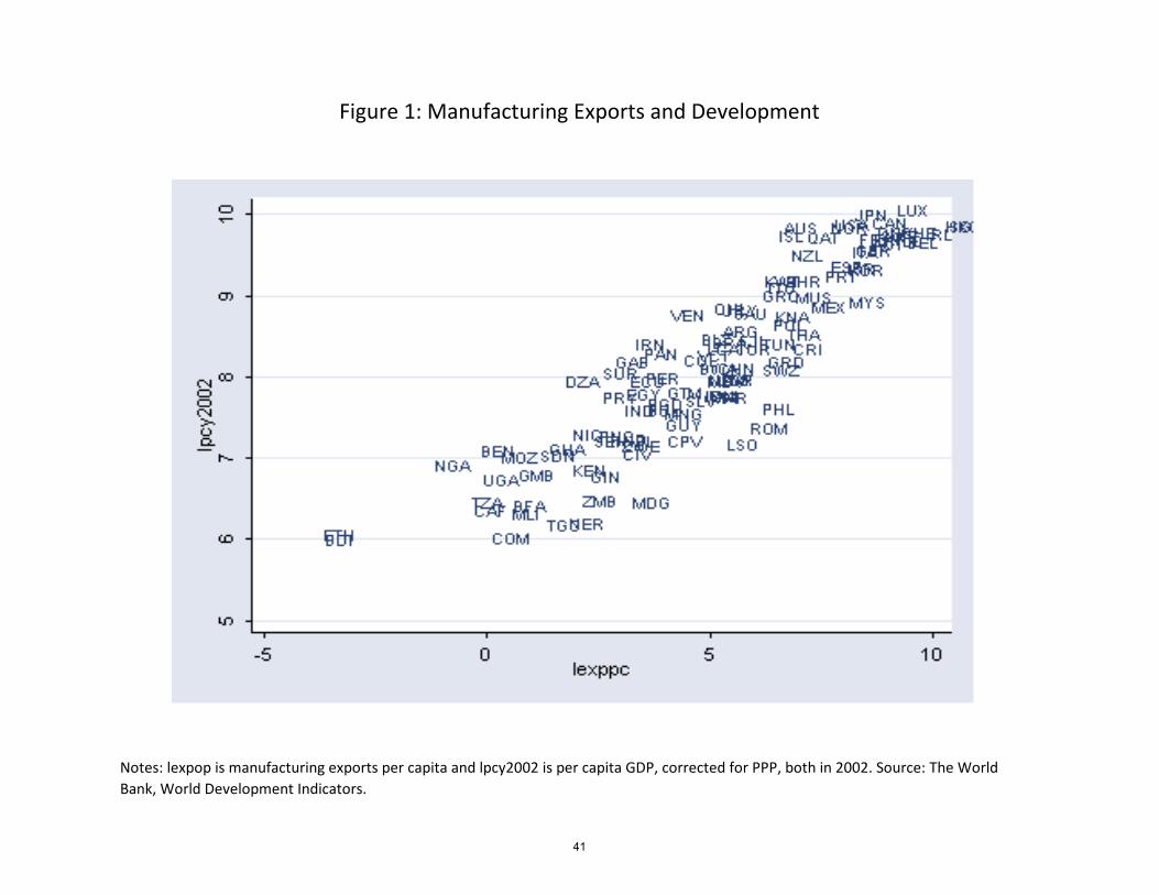
Figure 1: Manufacturing Exports and Development

Notes: lexpop is manufacturing exports per capita and lpcy2002 is per capita GDP, corrected for PPP, both in 2002. Source: The World Bank, World Development Indicators.

41

Figure 2: Export Values and Destinations

Notes: For each exporter, export values by product were assigned to bins acording to the number of destinations that product was exported to. Each bin was assigned the percent of total export value that it accounted for. The figure displays the percent of exports accounted for by products shipped to x destinations, averaged over all 151 exporters in the sample.

Average across exporters of percent of manufacturing export value accounted for by goods that have x destinations

0

2

4

6

8

10

12

14

1 2 3 4 5 6 7 8 9 10 11 12 13 14 15 16 17 18 19 20 21 22 23 24 25

x = Number of destinations for different goods

Perc

ent o

f tot

al m

anuf

actu

ring

expo

rt va

lue

42

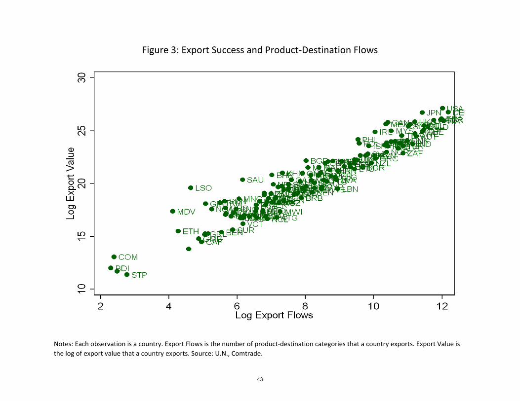
Figure 3: Export Success and Product-Destination Flows

Notes: Each observation is a country. Export Flows is the number of product-destination categories that a country exports. Export Value is the log of export value that a country exports. Source: U.N., Comtrade.

43

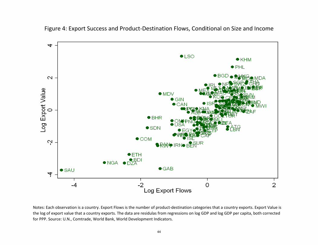
Figure 4: Export Success and Product-Destination Flows, Conditional on Size and Income

Notes: Each observation is a country. Export Flows is the number of product-destination categories that a country exports. Export Value is the log of export value that a country exports. The data are residulas from regressions on log GDP and log GDP per capita, both corrected for PPP. Source: U.N., Comtrade, World Bank, World Development Indicators.

44

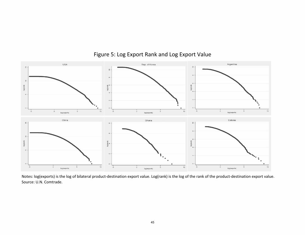
Figure 5: Log Export Rank and Log Export Value

Notes: log(exports) is the log of bilateral product-destination export value. Log(rank) is the log of the rank of the product-destination export value. Source: U.N. Comtrade.

45

Figure 6: Simulated Rank Graphs for Log Normal and mixed Pareto-Log Normal

Notes: The simulation for the log normal uses the empirical standard deviation of export values averaged over all 151 countries. The distribution of the mixed Pareto-log normal is defined in the text. The simulation uses the average estimated coefficients and standard deviations for all 151 countries from the estimation results below.

Pareto-Log Normal

Log Normal

46

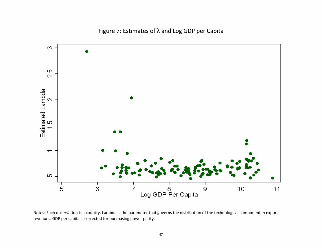
Figure 7: Estimates of λ and Log GDP per Capita

Notes: Each observation is a country. Lambda is the parameter that governs the distribution of the technological component in export revenues. GDP per capita is corrected for purchasing power parity.

47

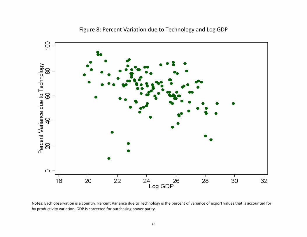
Figure 8: Percent Variation due to Technology and Log GDP

Notes: Each observation is a country. Percent Variance due to Technology is the percent of variance of export values that is accounted for by productivity variation. GDP is corrected for purchasing power parity.

48

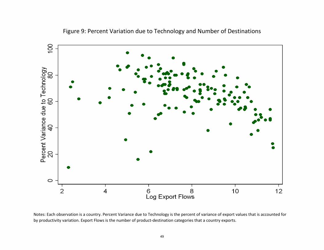
Figure 9: Percent Variation due to Technology and Number of Destinations

Notes: Each observation is a country. Percent Variance due to Technology is the percent of variance of export values that is accounted for by productivity variation. Export Flows is the number of product-destination categories that a country exports.

49