1

The Post-Crisis Slump in the Euro Area and the US: Evidence from an Estimated Three-Region DSGE Model

October 2015

Robert Kollmann (ECARES-ULB and CEPR)

Beatrice Pataracchia (European Commission, Joint Research Centre) Rafal Raciborski (European Commission, DG ECFIN)

Marco Ratto (European Commission, Joint Research Centre) Werner Roeger (European Commission, DG ECFIN)

Lukas Vogel (European Commission, DG ECFIN) The global financial crisis (2008-09) led to a sharp contraction in both Euro Area (EA) and US real activity, and was followed by a long-lasting slump. However, the post-crisis adjustment in the EA and the US shows striking differences—in particular, the EA slump has been markedly more protracted. We estimate a three-region (EA, US and Rest of World) New Keynesian DSGE model to quantify the drivers of the divergent EA and US adjustment paths. Our results suggest that the post-2009 EA slump mainly reflects adverse aggregate supply shocks (low TFP growth) and adverse shocks to capital investment. Fiscal austerity has not been a key driver of the EA slump. According to our estimates, the faster post-crisis rebound of the US economy largely reflects favorable investment shocks. Our estimates indicate small but non-negligible shock transmission between the EA and the US. The views expressed in this paper are those of the authors and should not be attributed to the European Commission

2

1. Introduction

The global financial crisis (2008-09) led to a sharp contraction in both Euro Area (EA) and US real

activity, and was followed by a long-lasting slump. However, the post-crisis adjustment in the EA

and the US shows striking differences. In particular, the EA slump has been markedly more

protracted. As of this writing, EA per capita real GDP remains below its pre-crisis peak. US per

capita GDP only recovered to its pre-crisis peak in 2014 and remains markedly below its pre-crisis

trend. Private investment contracted less (as a share of GDP) in the EA than in the US, during the

2008-09 crisis, but in the aftermath of crisis the EA investment share continued to trend down,

while the US investment rate began to recover in 2011. Post-crisis inflation has been lower in the

EA than in the US inflation. The EA wage share rose during the crisis, and remained elevated in the

aftermath of the crisis, while the US wage share trended downward. (See Section 2 for a detailed

discussion of the EA and US post-crisis dynamics.)

There is a heated debate about the causes of these developments. Some commentators argue

that the protracted EA slump reflects weak aggregate demand, driven i.a. by restrictive fiscal policy

(‘austerity’); see, e.g., International Monetary Fund (2012), De Grauwe (2014) and Stiglitz (2015).

Other analysts stress that rigidities in EA product and labor markets may have hampered the

rebound of the EA economy, by slowing down sectoral redeployment and the adoption of new

technologies (e.g., Fernald (2015)). Several commentators have also suggested that post-crisis

deleveraging pressures and financial constraints have contributed to the persistent slump (e.g.,

Rogoff (2015)): the much more rapid and aggressive non-conventional central bank policy during

and after the financial crisis (quantitative easing) in the US may have contributed to more rapid

deleveraging and balance sheet adjustment in the US (compared to the EA). The supply of credit to

the private sector may have been disrupted more persistently in the EA than in the US, due to the

continuing poorer health of EA banks. EA banks rebuilt their capital much more gradually than US

banks, after the crisis (OECD (2014)); in addition EA bank balance sheets were weakened by the

sovereign debt crisis that erupted in 2010/11 (Acharya et al. (2014), Kalemli-Özcan et al. (2015)).

The contribution of this paper is to shed light on these issues and hypotheses using a

state-of-the-art estimated dynamic stochastic general equilibrium (DSGE) model. So far, the

debate on the EA post-crisis slump has often been polemical, with remarkably little use of

evidence-based quantitative models. (Some recent research uses estimated DSGE models to

analyze the dynamics of the US economy since the crisis; see discussion below.) The use of an

estimated rich DSGE model allows us to recover the shocks that have driven the EA, US and ROW

3

economies—and, hence, we can determine what shocks and transmission mechanisms mattered

most and when.

In order to explain the striking post-crisis divergence between the EA and the US, we

jointly model these two ‘countries’, as well as an aggregate of the Rest of the World (ROW), i.e. we

consider a three-regions model. The EA and US blocks of the model have the same structure, but

parameters are allowed to differ across the blocks. The model is estimated using quarterly data for

the period 1999q1-2014q4. In order to address the range of views about the post-crisis slump (see

above), our model assumes a rich set of demand and supply shocks in goods, labor and asset

markets, and it allows for nominal and real rigidities and financial frictions.

Our estimation results suggest that the persistent EA slump reflects a combination of

adverse supply and demand shocks, in particular negative shocks to TFP growth (that already

began before the financial crisis) and adverse shocks to capital investment, linked to the continuing

poor health of the EA banking system. A key finding of our empirical analysis is that fiscal policy

(austerity) has not been a key driver of the EA slump. EA real activity has benefited from

noticeable positive factors during the aftermath of the crisis--however those positive influences

were weaker than the adverse supply and demand shocks mentioned above. For example, our

model estimates suggest that EA price and wage markups fell during and after the Great Recession,

which was reflected in a rise in the EA wage share, and was a driver of low post-crisis EA inflation.

The low post-crisis inflation in the EA is, hence, not primarily due to weak aggregate demand.

According to our estimates, the faster post-crisis rebound of the US economy largely

reflects lower investment risk premia, linked to the faster improvements in the health of the

financial system, in the aftermath of the financial crisis. Furthermore, TFP growth fell markedly

less in the US than in the EA. In the aftermath of the crisis, US aggregate activity also benefited

from more resilient private consumption demand, consistent with faster household deleveraging in

the US (compared to the EA). According to our estimates, US fiscal policy was more stimulative

than EA fiscal policy during the financial crisis. Our analysis also highlights the importance of

external factors: relatively strong ROW growth has stabilized US post-crisis growth. However, we

also identify important factors that slowed down the recovery of the US economy; in particular, US

price markups rose during the post-crisis period, which had a negative influence on US output (and

a positive effect on US inflation).

Our empirical estimates indicate non-negligible shock transmission between the EA and

the US. During the post-crisis period, low EA growth had a negative influence on US real activity.

4

Robust ROW growth in the aftermath of the financial crisis had a stronger positive effect on US

GDP growth than on EA growth.

As pointed out above, there is little empirical model-based research on the EA post-crisis

slump. By contrast, several recent papers have studied the post-crisis dynamics of inflation and real

activity in the US economy, using estimated closed economy DSGE models; see Christiano,

Eichenbaum and Trabandt (2015), Fratto and Uhlig (2015), Lindé, Smets and Wouters (2015) and

Del Negro, Giannoni and Schorfheide (2015). Like Fratto and Uhlig (2015) and Lindé et al. (2015)

we find that the zero-lower-bound (ZLB) was not a significant constraint for US and EA monetary

policy during the Great Recession and its aftermath. We concur with Christiano et al. (2015) that

financial shocks were the key driver of the Great Recession in the US; we find that those shocks

matter a great deal for the persistence of the EA slump. A key contribution of our analysis of the US

economy is that we model external (international) factors—we show that those factors play a

non-negligible role for the US recovery.

As pointed out above, a central contribution of the paper here is the estimation of a

large-scale multi-country model. By contrast most existing large multi-country models are

calibrated (e.g., Coenen et al. (2010)). Jacob and Peersman (2012), Kollmann (2013) have

estimated two-country DSGE models, but those models are much more stylized than the structure

here. The model here is closest to Kollmann, Ratto, Roeger in’t Veld and Vogel (2015) who

estimated a three-country model for Germany, the rest of the Euro Area and the ROW. That model

has a detailed German block, and the focus is on developments in that country, while the models of

other two regions are more stylized. By contrast, the model in the paper here treats the EA and US

at the same level of disaggregation, in order to understand differences in adjustment across these

two regions and in order to capture the interaction between these two regions.

Section 2 describes macroeconomic conditions in the EA, the US and ROW in the period

1999-2014. Section 3 gives an overview of the model. Section 4 discussed the econometric

approach. Section 5 presents the empirical results. Section 6 concludes.

2. EA and US macroeconomic conditions, 1999-2014

Figure 1 plots annual time series of key macroeconomic variables in the EA and the US in the

period 1999-2014, i.e. since the launch of the Euro. Unless stated otherwise, all data for the EA

5

pertain to the EA19 (all current members of the Euro Zone).1

Panels 1.a and 1.b show EA, US and ROW per capita real GDP (the series are normalized at

100 in 1999).2 The EA and the US grew at roughly the same rate (in per capita terms) before the

2008-09 Great Recession. The EA recession started slightly later than the US recession, but both

economies experienced approximately the same contraction (-5%) in 2008-09, and then began to

recover at roughly the same rate. However, the EA recovery was short-lived. In 2010-11 the

sovereign debt crisis erupted in EA periphery countries, and the trajectories of EA and US GDP

began to diverge: the EA experienced a recession in 2011- 2013, while US output growth returned

to pre-crisis rates. EA per capita GDP in 2014 remained 3% below the pre-crisis peak of 2007, and

20% below a linear trend fitted to 1995-2007 GDP. US real GDP stayed below its pre-crisis peak

until 2014, but remained about 10% below a (log-)linear trend fitted to 1995-2007 data. ROW per

capital GDP growth has markedly exceeded EA and US growth, during the sample period (see

Figure 1, Panel b.). ROW growth accelerated prior to the global crisis. In 2008-09 ROW growth

fell sharply, but remained positive; strong ROW growth (4%-5% p.a.) resumed in 2010.

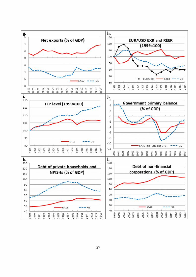
The EA-US divergence is also apparent in measured total factor productivity (TFP), see

Figure 1, Panel i. EA TFP fell during the Great Recession, and has since then stagnated at a level

below its pre-crisis peak. US TFP showed zero growth during the Great Recession, and then started

to grow again.

The contraction of the employment rate during the Great Recession was much sharper in

the US than in the EA (see Figure 1, Panel e). The US employment rate began to rebound in 2011,

but has not yet reached pre-crisis levels, while EA employment continued to slide down after the

crisis. The EA wage share (wage earnings/GDP ratio) trended downwards before 2007, and then

experiences a marked increase (by close to 4 percentage points) during the Great Recession that has

persisted to the end of the sample period (Panel f). By contrast, the US wage share followed a

downward trend throughout the sample period.

The dynamics of the components of aggregate demand too differs noticeably across the EA

1 Belgium, Germany, Estonia, Ireland, Greece, Spain, France, Italy, Cyprus, Latvia, Lithuania, Luxemburg, Malta, Netherlands, Austria, Portugal, Slovenia, Slovakia, and Finland. In 1999-2014 the EA19 accounted on average for 74% of total GDP of all 28 current members of the European Union. This paper focuses on the EA19 instead of EU28, as EA19 countries have a common monetary policy. The post-crisis recovery has been slower in the EA19 group than among non-EA members of the EU. Real GDP in the EA19 has grown, on average, by 1.4% p.a. in 1999-2014, while the rest of the EU28 has grown, on average, by 2.5% p.a. Real GDP in 2014 was still 1.2% below its 2008 level in the EA19, but 5.1% above the 2008 level in the group of non-EA EU28 countries. 2 RoW data are an aggregate of 58 countries, including non-EA EU28 Member States, countries that are neighbours of the EU28, G7 countries excluding EA member States and the U.S, and emerging markets. A detailed description of the construction of RoW series is provided in the data appendix.

6

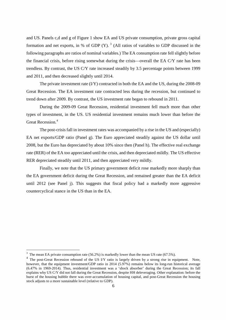
and US. Panels c,d and g of Figure 1 show EA and US private consumption, private gross capital

formation and net exports, in % of GDP (Y). 3 (All ratios of variables to GDP discussed in the

following paragraphs are ratios of nominal variables.) The EA consumption rate fell slightly before

the financial crisis, before rising somewhat during the crisis—overall the EA C/Y rate has been

trendless. By contrast, the US C/Y rate increased steadily by 3.5 percentage points between 1999

and 2011, and then decreased slightly until 2014.

The private investment rate (I/Y) contracted in both the EA and the US, during the 2008-09

Great Recession. The EA investment rate contracted less during the recession, but continued to

trend down after 2009. By contrast, the US investment rate began to rebound in 2011.

During the 2009-09 Great Recession, residential investment fell much more than other

types of investment, in the US. US residential investment remains much lower than before the

Great Recession.4

The post-crisis fall in investment rates was accompanied by a rise in the US and (especially)

EA net exports/GDP ratio (Panel g). The Euro appreciated steadily against the US dollar until

2008, but the Euro has depreciated by about 10% since then (Panel h). The effective real exchange

rate (RER) of the EA too appreciated until the crisis, and then depreciated mildly. The US effective

RER depreciated steadily until 2011, and then appreciated very mildly.

Finally, we note that the US primary government deficit rose markedly more sharply than

the EA government deficit during the Great Recession, and remained greater than the EA deficit

until 2012 (see Panel j). This suggests that fiscal policy had a markedly more aggressive

countercyclical stance in the US than in the EA.

3 The mean EA private consumption rate (56.2%) is markedly lower than the mean US rate (67.5%). 4 The post-Great Recession rebound of the US I/Y ratio is largely driven by a strong rise in equipment. Note, however, that the equipment investment/GDP ratio in 2014 (5.97%) remains below its long-run historical average (6.47% in 1969-2014). Thus, residential investment was a ‘shock absorber’ during the Great Recession; its fall explains why US C/Y did not fall during the Great Recession, despite HH deleveraging. Other explanation: before the burst of the housing bubble there was over-accumulation of housing capital, and post-Great Recession the housing stock adjusts to a more sustainable level (relative to GDP).

7

Recoveries after Major Recessions, real GDP (Y0=100)

Source: Priftis, Roeger & in’t Veld (2015)

3. Model description

We consider a three-country world consisting of the Euro Area (EA), the United States (US), and

the rest of the world (ROW). The EA and US blocks of the model are rather detailed, while the

ROW block is more stylized.5 The EA and US blocks assume two (representative) households,

firms and a government. EA and US households provide labor services to firms. One of the two

households in each country has access to financial markets, and she owns her country’s firms. The

other household has no access to financial markets, does not own financial or physical capital, and

simply consumes the disposable wage and transfer income in each period. We refer to the

household with financial market access and the household without financial market access as

‘Ricardian’ and ‘liquidity-constrained’ household, respectively. There is a sector producing

intermediate goods in the EA and the US that uses domestic labor and capital; the sector borrows

domestically and internationally. A final good sector in the EA and the US combines domestic and

imported intermediates and produces a homogeneous final good that is used for domestic

consumption, capital accumulation and exports. EA and US intermediate goods firms are

5The EA and U.S. blocks build on the QUEST model of the EU economy (Ratto et al., 2009). Other versions of that model have been estimated with US, with German, and with Spanish data (in 't Veld et al. (2011); Kollmann et al. (2014); in 't Veld et al. (2014)). The following presentation abstracts from adjustment costs (for labor and capital) and variable capital utilization rates assumed in the estimated model. These features help to better capture the data dynamics. Also, we only present the main exogenous shocks. The detailed model is available in a Not-for-Publication Appendix.

8

monopolists; EA and US wages are set by monopolistic trade unions. Nominal intermediate good

prices and wages are sticky. All other markets are competitive. Fiscal authorities in the EA and the

US levy distortive taxes and issue debt. We next present the key aspects of EA and US agents’

decision problems, and we then give an overview of the ROW model blocks. The EA and US

blocks have the same structure. The parameter values for the equations are country-specific as

determined in the estimation.

3.1. EA and US households

A household’s welfare depends on consumption and hours worked. Household h=r,l (r: Ricardian,

l: liquidity-constrained) period t utility, ,htU is: 1 11 1

11 1( ) (1 )h h h L ht t t t tU C C u Lσ κ

σ κη − −−− −≡ − + −

with 0 1η< <

and 0 , , .Ltuκ< h

tC and 1htL ≤ are consumption and the labor hours of worker h in period t,

respectively. There is habit persistence for consumption. The household’s time endowment is

normalized at 1, so that 1 htL− is the household’s leisure. L

tu is a country-specific exogenous

random preference shock. All exogenous random variables follow independent AR(1) processes.

The subjective discount factor of households , 1t tβ + is an exogenous random variable, with

, 10 1.t tβ +< < Date t expected life-time utility of household h, ,htV is defined by

, 1 1.h h h

t t t t t tV U E Vβ + += +

3.1.1. EA and US Ricardian household

The Ricardian household owns all domestic firms, and she holds one-period bonds issued by the

domestic government and foreign borrowers. The household’s period t budget constraint is:

1 1(1 ) (1 ) (1 ) (1 ) ,C r r g W g g W W W r i Kt t t t t t t t t t t t t t tp C T D e B r D r e B w L div divτ τ+ ++ + + + = + + + + − + + (1)

where 1gtD + and 1

WtB + are nominal holdings of domestic government debt and a foreign bond at

the end of date t; the interest rate earned on government bonds, ,gtr equals the policy rate plus a

spread, :gtspr g g

t t tr r spr= + (see also 3.4); the interest rate earned on foreign bonds, ,Wtr equals the

ROW policy rate plus a spread, :gtspr W RoW W

t t tr r spr= + ; te is the nominal exchange rate towards the

ROW. tp and tw are the final good price and the wage rate, respectively. Cτ is a (constant) tax

9

rate on consumption, while Wτ is the labor income tax rate; rtT is a lump-sum tax. I

tdiv and Ktdiv

are the dividends of the intermediate goods and investment good sectors.

3.1.2. EA and US liquidity-constrained household

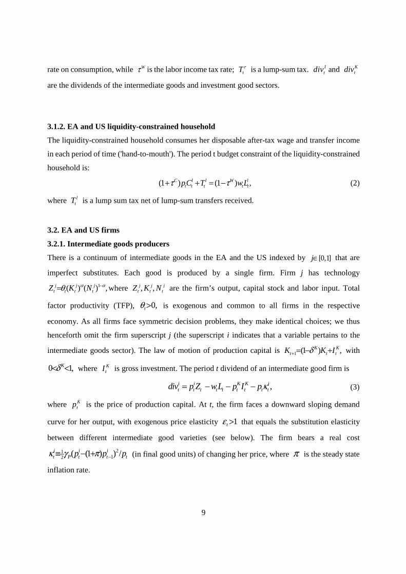
The liquidity-constrained household consumes her disposable after-tax wage and transfer income

in each period of time ('hand-to-mouth'). The period t budget constraint of the liquidity-constrained

household is:

(1 ) (1 ) ,C l l W lt t t t tpC T wLτ τ+ + = − (2)

where ltT is a lump sum tax net of lump-sum transfers received.

3.2. EA and US firms

3.2.1. Intermediate goods producers

There is a continuum of intermediate goods in the EA and the US indexed by [0,1]j∈ that are

imperfect substitutes. Each good is produced by a single firm. Firm j has technology 1( ) ( ) ,j j j

t t t tZ K Nα αθ −= where , ,j j jt t tZ K N are the firm’s output, capital stock and labor input. Total

factor productivity (TFP), 0,tθ > is exogenous and common to all firms in the respective

economy. As all firms face symmetric decision problems, they make identical choices; we thus

henceforth omit the firm superscript j (the superscript i indicates that a variable pertains to the

intermediate goods sector). The law of motion of production capital is 1 (1 ) ,K Kt t tK K Iδ+ = − + with

0 1,Kδ< < where KtI is gross investment. The period t dividend of an intermediate good firm is

,i i K K it t t t t t t t tdiv p Z wL p I pκ= − − − (3)

where Ktp is the price of production capital. At t, the firm faces a downward sloping demand

curve for her output, with exogenous price elasticity 1tε > that equals the substitution elasticity

between different intermediate good varieties (see below). The firm bears a real cost

2112 ( (1 ) ) /i i i

t P t t tp p pκ γ π −≡ − + (in final good units) of changing her price, where π is the steady state

inflation rate.

10

The firm maximizes the present value of dividends , 1 1 1( / ) ,i it t t t t t t tV div E p p Vρ + + += + where

, 1it tρ + is a stochastic discount factor that can differ from the intertemporal marginal rate of

substitution of the Ricardian household: , 1 , 1 1(1 ) / ,i i r r rt t t t t t tρ ε β λ λ+ + += + where i

tε is an exogenous

random variable with zero mean. The firm’s Euler equation for capital is:

, 1 1 1 1 11 ( / ){ / (1 ) / } ,i K K Kt t t t t t t t t t tE p p p MPK p p pρ δ+ + + + += + − +Ψ (4)

where 1 11 1 1( ) ( )t t t tMPK K Nα αθ α − −

+ + +≡ is the marginal product of capital at date t+1. The term tΨ

depends on the future marginal price-adjustment cost ( tΨ is zero, in steady state). itε induces

fluctuations in investment that are not related to (conventional) fundamentals; we thus refer to itε

as the ‘investment risk premium’ shock.

Price stickiness implies that the inflation rate of local intermediates, 1ln( / )i i it t tp pπ −≡ obeys an

expectational Phillips curve, 1 1( ) ( / ),i i i i i it t t t tE p MC ε

επ π ρ π π ϑ+ −− = − + − up to a linear approximation.

Here itMC is the marginal cost on intermediate good firms and /( 1)ε ε − is the steady state

mark-up factor. iρ is the steady state subjective discount factor of intermediate good firms, and

0iϑ > is a coefficient that depends on the cost of changing prices.

3.2.2. EA and US production of new capital goods

New capital is generated using final output. Let ( )K K K Kt t tJ Iξ=Ξ ⋅ be the amount of final output

needed to produce KtI units of production capital. Kξ is an increasing, strictly convex function,

while KtΞ is an exogenous shock. The price of production capital is '( ).K K K H

t t tp Iξ=Ξ The dividend

of the investment good sector is K K K Kt t t t tdiv p I p J= − .

3.2.3. EA and US final good sector

The final good is produced using the technology 1/ ( /( 1) 1/ ( 1)/ /( 1)(( ) ( ) (1 ) ( ) ) ,d dt t t t tD s Y s Mν ν ν ν ν ν ν ν− − −= + − with

0.5 1.dts< <

1 ( 1)/ /( 1)

0{ ( ) }t t t tj

t tY Z djε ε ε ε− −= ∫ is an aggregate of the local intermediates, where 1tε > is the

exogenous substitution elasticity between varieties; tM is a composite of intermediates imported

from the US or EA and the ROW. The home bias parameter dts is an exogenous random variable.

11

The price (=marginal cost) of the final good is 1 1 1/(1 )( ( ) (1 )( ) ) ,d i d mt t t t tp s p s pν ν ν− − −= + − where m

tp is the

import price index. The final good is used for domestic consumption and investment, and exported:

,r l Kt t t t t tD C C G J X= + + + + where tG and tX are government consumption and exports,

respectively.

3.3. Wage setting in the EA and the US

We assume a trade union that ‘differentiates’ homogenous labor hours provided by the two workers

into imperfectly substitutable labor services; the union then offers those services to intermediate

goods-producing firms--the labor input tN in those firms’ production functions is a CES

aggregate of these differentiated labor services. The union sets nominal wage rates of the

differentiated labor services to maximize the sum of the expected life-time utilities of the two

workers, subject to a quadratic cost of changing the wage rate. This implies that the (log) growth

rate of the nominal wage rate, 1ln( / ),wt t tw wπ −≡ obeys the wage Phillips curve,

1( ) ,w w w w wt t t w tE zπ π β π π λ+− = − + up to a (log-)linear approximation; here, wπ is steady state wage

inflation, and 0wλ > is a coefficient that depends on the cost of changing nominal wages; wtz is

the gap between a weighted average of workers’ marginal rates of substitution between

consumption and leisure, and the real wage rate. The model allows for inertia in the targeted real

wage, which is a weighted average of the workers’ marginal rates of substitution between

consumption and leisure augmented by a wage mark-up and the past real wage.

3.4. EA and US government

The period t government budget constraint is 1(1 ) ( )g g g W r lt t t t t t t tr D p G D w L Lτ++ + = + + +

( ) ,C r l r lt t t t tp C C T Tτ + + + where 1

gtD + is government debt; the interest rate paid by the government

equals the policy rate plus an exogenous spread, :gtspr .g g

t t tr r spr= +

Government consumption and lump-sum taxes respond to GDP growth and to public debt.

Real government consumption is set according to the following policy rule:

1

1 1 54( ) ( ln( / ) ) ( / ( ) ) ,G G G G G G G g g Gt t Y t t Y D t t t tc c c c Y Y g D p Y Dρ τ τ ε− − −− = − + − − − +

(5)

12

where /Gt t tc G Y≡ denotes government consumption normalized by real GDP, while Yg is the

steady state quarterly growth rate of GDP; Gtε is a white noise disturbance.6 Lump-sum taxes

follow an equivalent rule.

3.5. EA and US monetary policy

EA and US monetary policy are set as a function of inflation and GDP growth, according to an

interest rate feedback rule:

1 11 4 44 4(1 ) (1 )[ ( ln( / ) ) ( ln( / ) )] ,R R R R r R

t t t t Y t t Y tr r r P P Y Y gπρ ρ ρ τ π τ ε− − −= − + + − − + − + (6)

where tP and tY are the EA CPI and EA real GDP; Rtε is a white noise disturbance.

3.6. The ROW block

The model of the ROW economy is a simplified structure with fewer shocks. Specifically, the

ROW block consists of a New Keynesian Phillips curve, a budget constraint for the representative

household, demand functions for domestic and imported goods (derived from CES consumption

good aggregators), and a production technology that uses labor as the sole factor input. The ROW

block abstracts from capital accumulation. There are shocks to labor productivity, price mark-ups,

the subjective discount rate, the relative preference for domestic vs. imported goods, as well as

monetary policy shocks in the ROW.

3.7. Exogenous shocks

The estimated model assumes 67 exogenous shocks. Other recent estimated DSGE models

likewise assume many shocks (e.g., Kollmann (2013)), as it appears that many shocks are needed

to capture the key dynamic properties of macroeconomic and financial data. The large number of

shocks used here is also dictated by the fact that we use a large number of observables (54) for

estimation, to shed light on different potential causes for the post-crisis slump. Note that the number

of shocks has to be at least as large as the number of observables to avoid stochastic singularity of

the model.

6The estimated model also includes government investment; government capital raises the productivity of intermediate good producers.

13

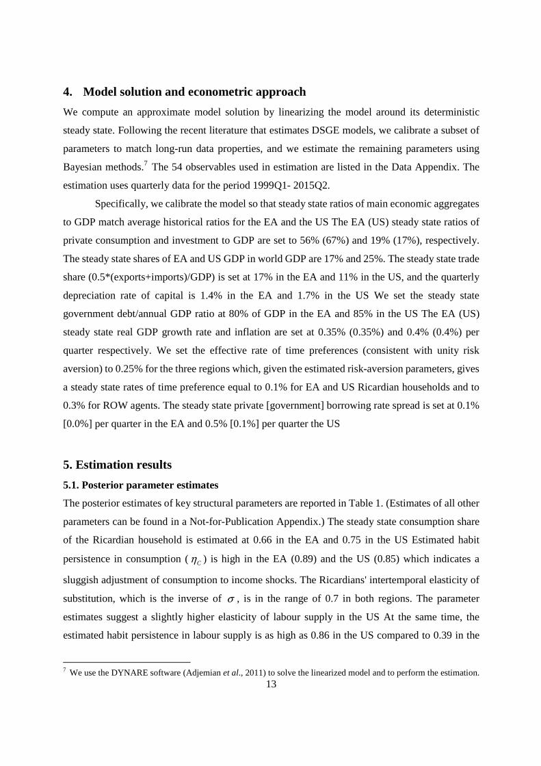
4. Model solution and econometric approach

We compute an approximate model solution by linearizing the model around its deterministic

steady state. Following the recent literature that estimates DSGE models, we calibrate a subset of

parameters to match long-run data properties, and we estimate the remaining parameters using

Bayesian methods.7 The 54 observables used in estimation are listed in the Data Appendix. The

estimation uses quarterly data for the period 1999Q1- 2015Q2.

Specifically, we calibrate the model so that steady state ratios of main economic aggregates

to GDP match average historical ratios for the EA and the US The EA (US) steady state ratios of

private consumption and investment to GDP are set to 56% (67%) and 19% (17%), respectively.

The steady state shares of EA and US GDP in world GDP are 17% and 25%. The steady state trade

share (0.5*(exports+imports)/GDP) is set at 17% in the EA and 11% in the US, and the quarterly

depreciation rate of capital is 1.4% in the EA and 1.7% in the US We set the steady state

government debt/annual GDP ratio at 80% of GDP in the EA and 85% in the US The EA (US)

steady state real GDP growth rate and inflation are set at 0.35% (0.35%) and 0.4% (0.4%) per

quarter respectively. We set the effective rate of time preferences (consistent with unity risk

aversion) to 0.25% for the three regions which, given the estimated risk-aversion parameters, gives

a steady state rates of time preference equal to 0.1% for EA and US Ricardian households and to

0.3% for ROW agents. The steady state private [government] borrowing rate spread is set at 0.1%

[0.0%] per quarter in the EA and 0.5% [0.1%] per quarter the US

5. Estimation results

5.1. Posterior parameter estimates

The posterior estimates of key structural parameters are reported in Table 1. (Estimates of all other

parameters can be found in a Not-for-Publication Appendix.) The steady state consumption share

of the Ricardian household is estimated at 0.66 in the EA and 0.75 in the US Estimated habit

persistence in consumption ( Cη ) is high in the EA (0.89) and the US (0.85) which indicates a

sluggish adjustment of consumption to income shocks. The Ricardians' intertemporal elasticity of

substitution, which is the inverse of σ , is in the range of 0.7 in both regions. The parameter

estimates suggest a slightly higher elasticity of labour supply in the US At the same time, the

estimated habit persistence in labour supply is as high as 0.86 in the US compared to 0.39 in the

7 We use the DYNARE software (Adjemian et al., 2011) to solve the linearized model and to perform the estimation.

14

EA. The parameter estimates of the trade block suggest high long-run price elasticity of overall

imports (ν ) in the EA (4.11) and the US (4.26). The elasticity of substitution is much lower

between imports of different origin ( 1ν ), namely 0.61 between US and RoW goods for the EA and

0.16 between EA and RoW goods for the US The model estimates also suggest substantial nominal

price and wage stickiness. Estimated price adjustment costs are lower in the EA, compared to the

US, whereas estimated wage stickiness is somewhat higher in the EA. The estimation points to

strong inertia in real wages. Estimated labour adjustment costs are higher in the US and investment

adjustment costs higher in the EA. Estimated monetary and fiscal parameters are very similar

across both regions. The model properties discussed in what follows are evaluated at the posterior

mode of the model parameters.8

5.2. Dynamic effects of shocks

Figure 3 shows dynamic responses to shocks that matter most during and after the financial crisis.

We begin by discussing shocks to EA and US aggregate supply (transitory and permanent TFP

shocks), and then consider household saving shocks as well as shocks to government consumption,

and to investment risk premia. Finally, we discuss interest parity shocks (between the ROW and the

EA/US), shocks to ROW competitiveness and shocks to ROW aggregate demand. In all cases, the

effects of a separate one-time 1% (0.01) innovations to a single exogenous variable are reported.

Predicted responses to transitory shocks to the level of TFP are standard, in the model here

(see Fig. 3a). A transitory positive country-specific TFP shock raises domestic GDP, consumption,

investment and the real wage rate, and it lowers domestic inflation, and depreciates the real

exchange rate, which induces a substitution of imports by domestic goods, and hence lowers

foreign output. Price stickiness, consumption habit and investment adjustment costs dampen the

expansion of aggregate demand, in the short term. This explains why, output rises much less (in

relative terms) than TFP, and why the transitory TFP shock lowers employment. The sluggish

adjustment of aggregate demand also explains why a positive TFP shock raises the trade balance of

the country that receives the shock.

The model also assumes serially correlated shocks to the growth rate of TFP. These shocks

trigger permanent level-shifts of the path of TFP. A positive permanent TFP (growth rate) shock

has a much stronger positive effect on domestic consumption, investment and output than a

8 We also computed model-implied statistics (impulse responses, variance decompositions and historical decompositions) at random parameter sub-draws of the Metropolis sample. Posterior means of those statistics are very close to statistics evaluated at the posterior mode of the model parameters (results available on request).

15

transitory shock (Fig. 3b). The stronger effects on permanent income and aggregate demand

explains why permanent TFP shocks raise hours worked and have a much more muted effect on

domestic inflation (than transitory TFP shocks). On impact, a permanent positive EA TFP shock

has only a very small negative effect on EA inflation. A permanent positive US TFP shock even

raises US inflation, in the short run.9 The much stronger effect of a permanent TFP shock on

aggregate demand also explains why that shock has a (slight) positive effect on foreign output.

These predicted responses suggest that transitory negative EA and US TFP shocks are not a

good candidate for explaining the salient facts about the Great Recession and its aftermath. A

transitory fall in TFP would raise inflation and employment and worsen the trade balance (which is

inconsistent with the observed fall in inflation and employment and the rise in the EA and US trade

balances after the Great Recession). A permanent negative TFP shock could be more in line with

the post-crisis data: such a shock is predicted by the model to lead to a persistent decline in output

and employment. However, while a permanent negative TFP shock is predicted to lower US

inflation, it generates a rise in EA inflation, which is inconsistent with the fall in EA inflation.

Furthermore, a permanent negative TFP shock fails to generate the strong decline in the

investment/GDP ratio seen in the post-crisis data, or a trade balance improvement.

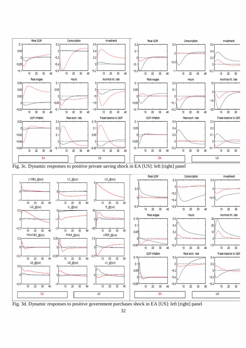
As shown in Fig. 3c, a positive shock to private saving (modeled as a positive shock to the

subject discount factor) lowers domestic consumption. The shock triggers a fall in domestic and

foreign GDP and inflation, it raises the trade balance, and it crowds in domestic and foreign

investment. Thus, while positive private saving shocks might have driven the fall in inflation and

the rise in trade balances, during/after the crisis, those shocks fail to account for the slump in

investment. Because of their predicted positive effect on investment, positive saving shocks

likewise fail to generate a persistent decline in GDP growth. Also, interestingly, a positive savings

shock is predicted to trigger an increase in the wage share in the EA and a decline in the US. This is

mainly due to the fact the EA has faster price adjustment but slower wage adjustment than the US.

Responses to fiscal shocks are standard. A rise in government purchases raises domestic

output, and has a small positive effect on foreign output (Fig. 3.d). Domestic and foreign

consumption and investment are crowded out by a rise in G. Thus, fiscal consolidation is a possible

9 The permanent US TFP shock boosts aggregate demand more than the EA shock. This reflects the fact that the US TFP growth rate is more persistent than EA TFP growth (autocorrelations: 0.97 and 0.95, respectively); see Table 2. Also, the steady state income share of forward-looking (Ricardian) households is higher in the US (0.75) than in the EA (0.66), while consumption habit persistence is slightly weaker in the US. Thus, a positive US TFP growth rate innovation stimulates aggregate demand more (than an EA growth shock), which explains the short-term rise in US inflation.

16

candidate for explaining the post-crisis output slump. However, the model-predicted crowding in

of consumption and investment generated by a fiscal consolidation seems inconsistent with the

actual slump in consumption and investment.

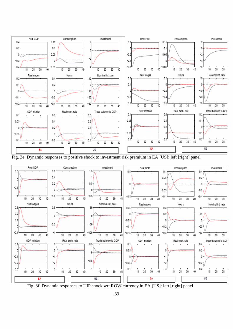
A rise in the investment risk premium is predicted to lower domestic investment, as well as

domestic and foreign output (Fig. 3e). The fall in aggregate demand induced by the shock lowers

labor demand, and thus employment and wages fall. Private consumption is crowded in by this

shock. In the short term, the shock lowers inflation. The investment risk premium thus generates

responses that are consistent along several dimensions with the post-crisis experience: it induces a

strong decline of investment relative to GDP; it also generates a highly persistent fall in GDP and a

decline in inflation.

Fig. 3f shows dynamic responses to an interest parity shock between the Euro and the ROW

currency, namely a fall in the risk premium on EA bonds (relative to ROW bonds). This shock

appreciates the Euro on impact against the ROW currency, as well as against the US dollar. In

response to this, the EA trade balance deteriorates (EA exports fall and EA imports rise). EA output

falls, but EA consumption and investment rise. The Euro appreciation is also accompanied by a fall

in EA inflation.

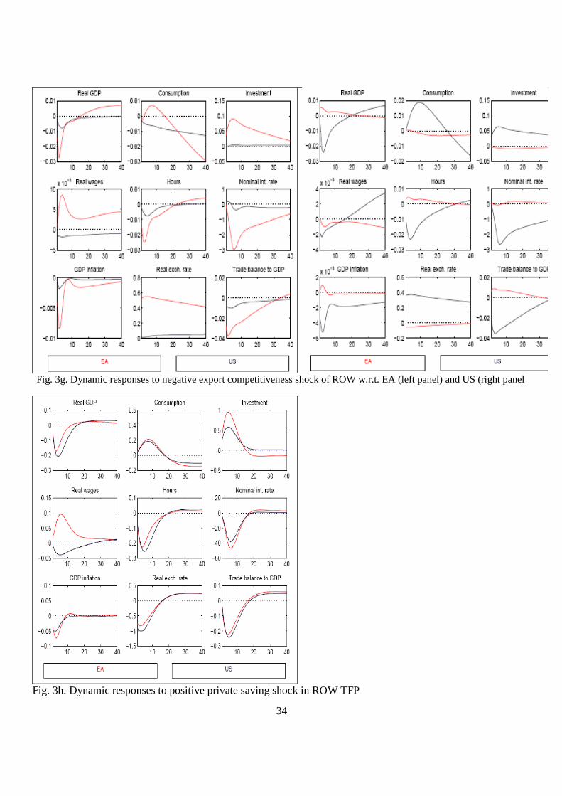
A fall in ROW export competitiveness in the EA (modeled as a fall in the export price

markup charged by ROW producers) raises EA imports, which boosts EA consumption and

investment (see Fig. 3g). EA inflation falls, the Euro depreciates, and EA output falls. Finally, Fig.

3h shows dynamic responses to a positive private saving shock in the ROW (i.e. a negative ROW

aggregate demand shock). That shock appreciates the EA and US real exchange rate, and it triggers

a fall in EA and US real GDP, a rise in EA and US consumption and investment, and a deterioration

in these countries’ trade balances.

Overall, ROW shocks are not prime candidates for explaining the sluggish EA and US

post-crisis recoveries. Their GDP impact on the EA and the US tends to be small, often resulting

from opposing effects of ROW shocks on domestic demand and the trade balance, i. e. opposing

income and competitiveness effects.

The results in this section suggest that only a combination of various shocks is required to

explain the major stylized facts of the EA and the US recovery. The next section disentangles the

various shocks using estimated historical shock decompositions.

17

5.3. Decomposing EA and US historical time series

To quantify the role of different shocks as drivers of endogenous variables, we plot the estimated

contribution of the different shocks to historical time series. Figure 2 shows historical

decompositions of the following EA and US variables: the year-on-year growth rate of GDP, the

year-on-year growth rate of the GDP deflator, the trade balance/GDP ratio, and the wage share.

The Figure plots historical series from which the sample averages have been subtracted. In each

sub-plot, the vertical black bars show the contribution of a different group of shocks (see below) to

the data, while stacked light bars show the contribution of the remaining shocks. Bars above the

horizontal axis represent positive shock contributions, while bars below the horizontal axis show

negative contributions. The sum of all shock contributions equals the historical data.

The decompositions of EA variables in Figure 2 plot the contributions of the following

(groups of) exogenous variables originating in the EA: (1) permanent and transitory shocks to EA

TFP; (2) EA fiscal policy shocks (innovations to the fiscal policy decision rules); (3) EA

monetary policy shocks; (4) EA price markup shocks; (5) interest parity shocks between the EA

and the ROW (‘Bond premium EA vs ROW’); (6) interest parity shocks between the US and the

ROW (‘Bond premium US vs ROW’); (7) shocks to the subjective rate of time preference of EA

households (‘Private saving shock’); (8) shocks to the EA risk premium on physical capital

(‘investment risk premium’); (9) shocks to EA wage markups and to the disutility of labor (‘labor

supply shocks’); (10) shocks to the relative preference for EA-produced versus imported goods and

price markup shocks for exports and imports (‘trade shocks’); (11) the remaining shocks

originating in the EA are less important than the shocks listed above, and are hence combined in a

category labelled ‘Others’. In addition, we show contributions of all other non-trade related shocks

that originate in the US (‘Shocks US’), and that originate in the ROW (‘Shocks ROW’).

Shock decompositions for US variables use an analogous grouping of shocks (i.e. we also

consider 9 groups of shocks that originate in the US etc.).

The historical shock decompositions for the period 1999-2014 suggest that a physical

investment boom was under way before the Great Recession and that this was an important factor

lifting GDP above trend before 2009, in both the EA and the US. (We estimate a string of negative

shocks to the investment risk premia that raised investment above the levels predicted by

conventional macro-fundamentals). Beginning in 2008, important adverse shocks occurred.

18

Decomposing EA time series

As shown in Fig. 2a, the EA growth slowdown in 2009 is largely due to: (i) an increase in the risk

premium on investment; (ii) a decline in TFP growth that represents a permanent level shift; (iii)

negative trade shocks. This was followed in 2010 by a relatively rapid partial recovery due to a fall

in risk premia (possibly linked to policy measures to stabilize the financial system) and because of

positive ROW developments. However, in 2011 the EA was hit by a further rise in the investment

risk premium, with an adverse effect on investment and GDP. We interpret this second dip in real

activity as a consequence of the sovereign debt crisis that weakened EA bank balance sheets, and

thus reduced the supply of credit to the corporate sector and to households, thus lowering corporate

investment and household (residential) investment.10

Shocks to EA price and wage markups were less important than TFP and investment risk

premium shocks for the post-2009 dynamics. Negative household saving shocks lowered EA GDP

growth in the aftermath of 2009; however, those shocks did not play an important role for EA GDP.

(The effect of higher saving on GDP is subdued because it triggers fall in the interest rate which

stabilizes domestic demand, and because it improves the trade balance; see Section 5.2.) Positive

growth contributions from other sources have been very limited after 2009. Strong ROW growth

had a small positive spillover effect on EA growth. We also identify a small increase in the external

Euro risk premium that generated a modest growth impulse via Euro depreciation. Our model

estimates suggest that shocks originating in the US and in the ROW had a small but noticeable

effect on EA GDP growth. In particular, US shocks raised EA growth in the first half of the 2000s,

and US shocks lowered EA growth during the Great Recession. However, the influence of US

shocks on EA GDP was negligible in the aftermath of the Great Recession. EA fiscal policy shocks

had a slight stimulative effect during the Great Recession, but EA fiscal policy had a negligible

influence on EA GDP during the aftermath of the crisis. Fiscal ‘austerity’ is not to blame for the EA

post-crisis slump. 11

10 Kalemli-Özcan et al. (2015) for provide micro evidence on this transmission channel of the sovereign debt crisis. 11Estimated monetary policy shocks (disturbances to the interest rate rule) are positive in 2014, when the EA policy rate was close to zero. This suggests that the zero lower bound (ZLB) on the policy rate was binding then (the policy rate implied by the policy rule, without disturbance, is negative in 2014, so that a positive interest rate disturbance is needed to match the observed policy rate). These positive monetary policy shocks explain why the historical decompositions show that EA monetary policy shocks had a negative effect on the EA GDP growth rate, at the end of the sample period. We estimate a linearized version of the model in which the ZLB is not imposed as a constraint on policy. Estimation of a rich model such as ours with an occasionally binding ZLB constraint is not feasible. However, omission of the ZLB constraint may not be an issue for our main results, as the ZLB was most likely only binding at the very end of the sample. However, the omission of the ZLB implies that our model simulations may understate the

19

The investment shock not only is important for explaining EA GDP growth but is needed to

explain large fluctuations in investment, which are not explained by fundamentals (see Section 5.2,

where we showed that investment risk premium shocks are the prime driver of real

investment).The investment risk premium shock also helps to explain the dynamics of the EA trade

balance before and after 2009 (see Fig. 2c). The investment risk premium contributed furthermore

noticeably to the rise in the EA wage share after 2009 (see Fig. 2d).12

Negative permanent TFP shocks are important for explaining the post-crisis slump, as those

shocks are the only driver that can generate the observed persistent downward level shift of GDP.

Investment premium shocks too can generate persistent GDP responses, however to match the

observed in EA GDP an investment shock would be needed that would far exceed the observed fall

in EA investment. Thus, a combination of adverse TFP shocks and risk premium shocks (in

combination with a pre-crisis investment boom) can account for the slow post 2009 growth in the

EA. As already shown in the previous section, the savings and the fiscal shock cannot generate the

magnitude of the GDP decline because of offsetting movements in other demand components. The

savings shock (together with the risk premium shock) is however important for explaining the

slowdown of inflation in the EA (Fig. 2b). Falling import prices (including oil prices) are another

important factor explaining low EA inflation in the aftermath of the crisis.

Decomposing US time series

Investment risk premium shocks are even more dominant for US GDP growth (see Fig. 2a): those

shocks account almost fully for the 2008-09 output contraction. Importantly, the adverse

investment risk premium shock was much more short-lived in the US than in the EA. This is the

main factor that explains the better post-crisis GDP performance of the US.

impact of fiscal shocks on real activity, at the end of the sample. To assess the size of the bias, the Appendix compares impulse responses of a government purchases shock with and without the ZLB constraint (the simulations with ZLB constraint use the Guerrieri and Iacoviello (2014) algorithm). We assume there that agents expect the ZLB to bind over a period of 2 years (a frequent assumption in comparable exercises; see e.g. Coenen et al. (2012)). With an expected ZLB constraint of 2 years, the fiscal multiplier rises by about half, and there is less crowding in of domestic demand. Also the trade balance improves less, because the increase in the real interest rate initially leads to a real appreciation, followed by a depreciation. However, the predicted responses to estimated government purchases shocks remain very modest (those responses are already very weak in the model simulations without ZLB shocks). 12 As documented above, the EA wage share fell before the Great Recession, and then rose markedly and persistently during the Great Recession. The model largely interprets this as reflecting a rise in in the price markup charged by EA firms before the Great Recession, followed by a fall in the price markup during the Great Recession. As discussed below, the negative post-GR EA markup shocks have also been a key contributor to low post-GR inflation in the EA. The negative TFP shocks in the EA too contributed to a rise in the wage share (given the wage and employment rigidities in the EA); see Figure 1.e.

20

Various factors could play a role for explaining the different post crisis evolutions of EA

and US investment risk premia. The supply of credit to the private sector may have been disrupted

more persistently in the EA than in the US, due to the continuing poorer health of EA banks. Policy

measures relieving the banking sector from bad loans (various QE measures) were pursued earlier

and more aggressively in the US. As a result, US banks rebuilt their capital much faster than EA

banks, after 2008-09 (OECD (2014)); also, US banks were not weakened by the sovereign debt

crisis. Faster household deleveraging in the US (see Fig. 1.k) also supports the idea that investment

frictions fell more rapidly in the US.

Private saving shocks and price mark-up shocks too contributed noticeably to the US output

collapse in 2008-09. We interpret the US saving shock as a proxy for the strong household debt

deleveraging that began in 2009 (see Fig. 1.k).13 Household savings shocks are also very important

for explaining the fall of US inflation in 2009. (By contrast, the effect of saving shocks on GDP and

inflation is much less important in the EA). In the aftermath of the 2008-09 recession, inflation

recovered faster in the US than in the EA. The temporary nature of the investment shock

contributed to the rapid fall of inflation in 2009 and its subsequent recovery. Positive shocks to US

price and wage markups too contributed the rebound of inflation. The rise in price mark-ups is also

the most important factor explaining the decline in the US wage share after 2009. The temporary

nature of the US investment risk premium shock coincides well with the temporary increase of the

trade balance. The size and persistence of the savings shock in isolation would have led to a bigger

and more persistent increase of the US trade balance. However, this effect was largely offset by

negative shocks from the EA and the ROW. Finally, we note that US fiscal policy was more

stimulative than EA fiscal policy during the Great Recession; however after the Great Recession,

the stance of US fiscal policy gradually became less expansionary, which put downward pressure

on US GDP growth.14

6. Conclusion

We have estimated a three-region (EA, US and Rest of World) New Keynesian DSGE model to

quantify the drivers of the divergent EA and US adjustment paths during the aftermath of the global

financial crisis. Our analysis reveals that the slow post-crisis recoveries in the US and EA have

both common and idiosyncratic components. An important common feature is the strong rise in

13 The rapid adjustment of US household debt is consistent with Albuquerque et al. (2014) who estimate that debt adjustment was completed in 2012 in the US. 14 Other adverse shocks that hampered the post-crisis rebound of US real activity included negative trade shocks (like for the EA). Also, shocks originating in the EA had an adverse effect on US growth in the post-GR era.

21

investment risk premia during the 2008-09 recession that put an end to a pre-crisis investment

boom. Our model estimates suggest that negative post-2009 investment shocks have been more

persistent in the EA than in the US. These model-based estimates are consistent with various

performance indicators of the EA and US financial/banking systems. An important additional

contributing factor of the post-2009 EA slump has been the slowdown of TFP growth. Private

saving shocks and fiscal austerity are less important for explaining low EA growth according to our

estimates, however, private saving shocks are important for the slowdown of inflation. Our

estimates indicate small but non-negligible shock transmission between the EA and the US.

22

References Albuquerque, Bruno, Ursel Bachmann and Georgi Krustev, 2014. Has US Household

Deleveraging Ended? A Model-Based Estimate of Equilibrium Debt. ECB Working Paper 1643. Christiano, L., M. Eichenbaum and M. Trabandt, 2015. Understanding the Great Recession.

American Economic Journal: Macroeconomics 7, 110–167. Coenen, Günter, Giovanni Lombardo, Frank Smets and Roland Straub, 2010. International

Transmission and Monetary Policy Cooperation. In: International Dimensions of Monetary Policy, Jordi Gali and Mark Gertler (eds), NBER, Cambridge, M.A., Chapter 3, pp. 157-192.

Coenen, G., Erceg, C., Freedman, C., Furceri, D., Kumhof, M., Lalonde, R., Laxton, D., Lindé, J., Mourougane, A., Muir, D., Mursula, S., de Resende, C., Roberts, J., Roeger, W., Snudden, S., Trabandt, M., in’t Veld, J., 2012. Effects of fiscal stimulus in structural models. American Economic Journal: Macroeconomics 4, 22–68.

De Grauwe, Paul, 2014. Stop structural reforms, start public investments. Del Negro, M., M. Giannoni and F. Schorfheide, 2015. Inflation in the Great Recession and New

Keynesian Models, American Economic Journal: Macroeconomics 7, 168-196. Fernald, J., 2015. The Pre-Global-Financial-Crisis Slowdown in Productivity. Working Paper. Fratto, C. and H. Uhlig, 2014. Accounting for Post-Crisis Inflation and Employment: A Retro

Analysis, NBER Working Paper 20707. Guerrieri, L. and M. Iacoviello, 2014. OccBin: A Toolkit for Solving Dynamic Models With

Occasionally Binding Constraints Easily, Journal of Monetary Economics. International Monetary Fund, 2012. World Economic Outlook (October). in’t Veld, Jan, Robert Kollmann, Beatrice Pataracchia, Marco Ratto and Werner Roeger, 2014.

International Capital Flows and the Boom-Bust Cycle in Spain. Journal of International Money and Finance 48, 314-335.

Kalemli-Ozcan, Sebnem, Luc Laeven and David Moreno, 2014. Debt Overhang in Europe: Evidence from Firm-Bank-Sovereign Linkages. Working Paper, University of Maryland.

Kollmann, Robert, Jan in’t Veld, Marco Ratto, Werner Roeger and Lukas Vogel, 2015. What Drives the German Current Account? And How Does it Affect Other EU Member States? Economic Policy 40, 47-93.

Kollmann, Robert, 2013. Global Banks, Financial Shocks and International Business Cycles: Evidence from an Estimated Model, Journal of Money, Credit and Banking 45 (S2), 159-195.

Lindé, J., F. Smets and R. Wouters, 2015. Challenges for Macro Models Used at Central Bank. Working Paper.

OECD, 2014. Economic Surveys: Euro Area. Ratto M., W. Roeger and J. in ’t Veld, 2009. ‘QUEST III: an estimated open-economy DSGE

model of the Euro Area with fiscal and monetary policy’, Economic Modelling, 26, 222–33. Rogoff, K., 2015. Debt Supercycle, Not Secular Stagnation. VoxEU. Stiglitz, Joseph, 2015. Les dégâts induits par la crise sont durables. In: Le Soir (Bruxelles).

September 2, 2015, pp.14-15.

23

Table 1. Prior and posterior distributions of key estimated model parameters Posteriors Priors EA US Mode Std Mode Std Distribution Mean Std (1) (2) (3) (4) (5) (6) (7) Preferences Consumption habit ηC 0.89 0.03 0.85 0.03 Beta 0.5 0.2Labour habit ηL 0.39 0.22 0.86 0.08 Beta 0.5 0.2Risk aversion σ 1.41 0.17 1.39 0.17 Gamma 1.5 0.2Labor supply κ 2.31 0.45 2.14 0.41 Gamma 2.5 0.5Import price elasticity ν 4.11 0.43 4.26 0.45 Gamma 2 1Import source elasticity ν1 0.60 0.22 0.16 0.07 Gamma 2 1Oil demand elasticity νO 0.33 0.02 0.33 0.03 Beta 0.5 0.08Nominal and real frictions NLC household share sr 0.66 0.05 0.75 0.02 Beta 0.65 0.05Price adj. cost γP 28.6 6.64 62.2 14.8 Gamma 60 40Forward-looking prices sfp 0.54 0.04 0.77 0.05 Beta 0.5 0.1Import price rigidity ρPM 0.24 0.10 0.19 0.10 Beta 2 0.8Nominal wage adj. cost γW 4.84 1.33 2.94 0.83 Gamma 5 2Forward-looking wages sfw 0.52 0.10 0.51 0.11 Beta 0.5 0.1Real wage rigidity ρw 0.96 0.01 0.96 0.01 Beta 0.5 0.2Import demand inertia ρM 0.33 0.06 0.45 0.05 Beta 0.7 0.1Oil demand inertia ρO 0.26 0.08 0.19 0.05 Beta 0.7 0.1Labour adj. cost γL 4.69 1.01 12.1 3.60 Gamma 60 40Capital adj. cost γK 41.8 22.6 51.9 22.2 Gamma 60 40Investment adj. cost γI 91.2 31.5 49.2 21.3 Gamma 60 40Capacity util. adj. cost γUC 0.04 0.02 0.07 0.02 Gamma 0.1 0.04Monetary policy Interest persistence ρR 0.87 0.02 0.85 0.03 Beta 0.7 0.12Response to inflation τR,π 2.37 0.37 2.09 0.31 Beta 2 0.4Response to GDP τR,y 0.02 0.01 0.02 0.00 Beta 0.5 0.2Fiscal policy Transfer persistence ρT 0.97 0.01 0.97 0.01 Beta 0.7 0.1Response to deficit τT,d 0.01 0.00 0.01 0.00 Beta 0.03 0.008Response to debt τT,b 0.00 0.00 0.00 0.00 Beta 0.001 0.001Consumption persistence ρGC 0.95 0.01 0.95 0.02 Beta 0.7 0.1Investment persistence ρIG 0.83 0.05 0.92 0.02 Beta 0.7 0.1

24

Table 2. Prior and posterior distributions of key estimated EA and US shock processes Posteriors Priors EA US Mode Std Mode Std Distribution Mean Std (1) (2) (3) (4) (5) (6) (7) AR(1) coefficients Temporary TFP ρAY 0.69 0.10 0.54 0.10 Beta 0.5 0.2Permanent TFP ρGAY 0.95 0.02 0.97 0.01 Beta 0.85 0.075Private savings ρUC 0.79 0.05 0.77 0.05 Beta 0.5 0.2Investment risk ρRK 0.83 0.05 0.87 0.04 Beta 0.5 0.2Foreign risk ρRE 0.79 0.06 0.69 0.09 Beta 0.5 0.2Price mark-up ρP 0.00 0.00 0.75 0.11 Beta 0.5 0.2Taxation ρTAX 0.77 0.08 0.86 0.05 Beta 0.5 0.2Trade share ρM 0.94 0.02 0.90 0.02 Beta 0.5 0.2Bilateral trade ρM1 0.56 0.19 0.57 0.21 Beta 0.5 0.2Oil share ρO 0.33 0.35 0.54 0.21 Beta 0.5 0.2Export price ρPX 0.95 0.01 0.85 0.04 Beta 0.5 0.2RoW export price ρPX 0.99 0.00 0.98 0.00 Beta 0.5 0.2Innovations Temporary TFP σAY 0.01003 0.00146 0.01428 0.00210 Gamma 0.005 0.002Permanent TFP σGAY 0.00029 0.00009 0.00031 0.00000 Gamma 0.0002 0.00008Private savings σUC 0.01265 0.00387 0.01401 0.00451 Gamma 0.01 0.004Investment risk σRK 0.01142 0.00313 0.00985 0.00287 Gamma 0.01 0.004Foreign risk σRE 0.00265 0.00071 0.00356 0.00100 Gamma 0.01 0.004Price mark-up σP 0.04510 0.00894 0.04001 0.01005 Gamma 0.02 0.008Labour supply σL 0.01190 0.00295 0.01839 0.00409 Gamma 0.01 0.004Labour demand σW 0.01021 0.00507 0.00909 0.00415 Gamma 0.01 0.004Monetary policy σM 0.00095 0.00009 0.00125 0.00012 Gamma 0.01 0.004Gov. consumption σGC 0.00066 0.00005 0.00133 0.00012 Gamma 0.01 0.004Gov. investment σIG 0.00120 0.00010 0.00072 0.00006 Gamma 0.01 0.004Gov. transfers σTR 0.00103 0.00009 0.00240 0.00023 Gamma 0.01 0.004Taxation σTAX 0.01176 0.00226 0.01843 0.00286 Gamma 0.01 0.004Trade share σM 0.05514 0.00706 0.08631 0.00977 Gamma 0.02 0.008Bilateral trade σM1 0.02335 0.00835 0.01207 0.00435 Gamma 0.02 0.008Oil share σO 0.02647 0.00885 0.01685 0.00647 Gamma 0.02 0.008Export price σPX 0.00613 0.00056 0.00807 0.00072 Gamma 0.01 0.004RoW export price σPM 0.04523 0.00397 0.05819 0.00518 Gamma 0.01 0.004

25

Table 3. Prior and posterior distributions of key estimated RoW shock processes Posteriors Priors Mode Std Distribution Mean Std (1) (2) (3) (4) (5) AR(1) coefficients Phillips curve ρY 0.30 0.18 Beta 0.5 0.2 Private savings ρUC 0.83 0.05 Beta 0.5 0.2 Trade share ρM 0.92 0.05 Beta 0.5 0.2 Bilateral trade ρM1 0.98 0.00 Beta 0.5 0.2 Oil price ρPO 0.88 0.05 Beta 0.85 0.075 Innovations Phillips curve σY 0.00451 0.00186 Gamma 0.01 0.004 Private savings σUC 0.00879 0.00299 Gamma 0.01 0.004 Monetary policy σM 0.00164 0.00046 Gamma 0.01 0.004 Trade share σM 0.02565 0.00469 Gamma 0.02 0.008 Bilateral trade σM1 0.01045 0.00129 Gamma 0.02 0.008

26

a.

b.

c.

d.

e.

f.

27

g.

h.

i.

j.

k.

l.

28

m.

n.

EA, Bank nonperforming loans/total gross loans (%). Source: World Bank

o.

US, Bank nonperforming loans/total gross loans (%). Source: World Bank

Fig. 1. Macroeconomic conditions in the EA19, US and ROW Notes: Employment rate is total employment (persons) to working-age (15-64) population. The wage share is compensation of employees adjusted for the imputed compensation of self-employed in per cent of GDP at factor costs. An increase in the EUR/USD rate corresponds to EUR depreciation against the USD; a REER increase corresponds to real effective appreciation in the respective region. EA19 government balance exclude Greece and Lithuania due to missing data. REER is based on HICP and a group of 42 countries. Private debt: end-of-year debt of domestic households and non-financial corporations for the EA18 and the US.

0

0.5

1

1.5

2

2.5

3

3.5

1999

2000

2001

2002

2003

2004

2005

2006

2007

2008

2009

2010

2011

2012

2013

2014

% inflation (GDP deflator)

EA19

US

29

Fig. 2a. Historical decompositions of real GDP growth rate (year-on-year) in EA [US]: left [right] panel

Fig. 2b. Historical decompositions of growth rate (YoY) of GDP deflator in EA [US]: left [right] panel

30

Fig. 2c. Historical decompositions of trade balance/GDP ratio in EA [US]: left [right] panel

Fig. 2d. Historical decompositions of labor share in EA [US]: left [right] panel

31

Fig. 3a. Dynamic responses to a transitory positive TFP shock in EA [US]: left [right] panel

Fig. 3b. Dynamic responses to a positive permanent TFP (growth rate) shock in EA [US]: left [right] panel

32

Fig. 3c. Dynamic responses to positive private saving shock in EA [US]: left [right] panel

Fig. 3d. Dynamic responses to positive government purchases shock in EA [US]: left [right] panel

33

Fig. 3e. Dynamic responses to positive shock to investment risk premium in EA [US]: left [right] panel

Fig. 3f. Dynamic responses to UIP shock wrt ROW currency in EA [US]: left [right] panel

34

Fig. 3g. Dynamic responses to negative export competitiveness shock of ROW w.r.t. EA (left panel) and US (right panel

Fig. 3h. Dynamic responses to positive private saving shock in ROW TFP

35

APPENDIX 1. DATA 1. Data sources Data for the EA19 (quarterly national accounts, fiscal aggregates, quarterly interest and exchange rates) are taken from Eurostat. Corresponding data for the US come from the Bureau of Economic Analysis (BEA) and the Federal Reserve. Quarterly data is used where available. In the remaining cases annual series are interpolated. The disaggregation of total in bilateral trade flows is based on trade shares from the GTAP trade matrices for trade in goods and services. RoW series are constructed on the basis of the IMF International Financial Statistics (IFS) and World Economic Outlook (WEO) databases. The construction of RoW series is described below. 2. Constructing data series for ROW variables Series for GDP and prices in the RoW starting in 1999 are constructed on the basis of data for the following 58 countries: Albania, Algeria, Argentina, Armenia, Australia, Azerbaijan, Belarus, Brazil, Bulgaria, Canada, Chile, China, Colombia, Croatia, Czech Republic, Denmark, Egypt, Georgia, Hong Kong, Hungary, Iceland, India, Indonesia, Iran, Israel, Japan, Jordan, Korea, Lebanon, Libya, FYR Macedonia, Malaysia, Mexico, Moldova, Montenegro, Morocco, New Zealand, Nigeria, Norway, Philippines, Poland, Romania, Russia, Saudi Arabia, Serbia, Singapore, South Africa, Sweden, Switzerland, Syria, Taiwan, Thailand, Tunisia, Turkey, Ukraine, United Arab Emirates, United Kingdom, and Venezuela. The data are annual data and taken from the IMF International Financial Statistics (IFS) and World Economic Outlook (WEO) databases. The series for RoW real GDP (GDPR) is constructed as follows. First, we normalise the series for GDP in national currency (NAC) at constant prices for each country (i) at the common base year t=0:

10 1

( )i i

tt ki ik

k

GDPR GDPR

GDPR GDPR=−

= ∏

Then we calculate the time-varying share of each country in the block based on nominal GDP (GDPN) in USD. Finally, we compute RoW GDPR as the GDPN-weighted average of the 58 countries, which gives the RoW GDPR index with base year t=0:

,58

,1

USD iRoW itt tUSD RoWi

t

GDPNGDPR GDPR

GDPN==∑

The aggregation applies time-varying weights in order to account for changes in the relative economic weight of individual RoW countries over the sample period. RoW GDPR is normalised to 1 in year 2005. The series for the RoW GDP deflator (PGDP) is constructed analogously to the RoW GDPR series. First, we normalise the series for the PGDP for each country (i) to base year t=0:

10 1

( )i i

tt ki ik

k

PGDP PGDP

PGDP PGDP=−

= ∏

Then we calculate the time-varying share of each country in the block based on GDP in USD and compute the ROW PGDP as the GDP-weighted average of the 58 country series, which gives the RoW GDPR index with base year t=0:

,58

,1

USD iRoW it

t tUSD RoWit

GDPNPGDP PGDP

GDPN==∑

36

RoW GDPR is normalised to 1 in year 2005. An index of RoW nominal GDP (GDPN) with base year 2005 can be calculated by multiplying RoW GDPR with RoW PGDP. The RoW block in the model has a flexible nominal exchange rate. The ROW nominal exchange rate to the USD (e) is calculated as GDP-weighted average of bilateral exchange rates against the USD for the 58 countries. As for GDPR and PGDP above, we normalise bilateral USD exchange rates in each country to the base year t=0:

,$ ,$

,$ ,$10 1

( )i i

tt ki ik

k

e e

e e=−

= ∏

The RoW nominal exchange rate to the USD with base year t=0 is then calculated as GDP-weighted average of the 58 country series:

,$58,$ ,$

,$1

iRoW itt tRoWi

t

GDPNe e

GDPN==∑

The RoW exchange rate to the USD is normalised to 1 in 2005. The exchange rate series includes exchange rate movements between members of the RoW group instead of attributing them to the RoW price index. The short-term interest rate for the RoW is the GDP-weighted average of interest rate series for countries (i) in the RoW. The sample is reduced to 47 countries due to limited data availability and the GDP weights are adjusted accordingly. The RoW trade balance (TB) balances international trade flows:

( )RoW EA USt t tTB TB TB= − +

RoW exports equal the sum of EA19 and US imports from the RoW. The bilateral imports from the RoW are obtained by subtracting imports from the US (EA19) from total EA19 (US) imports based on trade matrices for international good and service trade. Analogously, imports of the RoW equal EA19 plus US exports to the RoW. 3. List of observable variables We observe the following 23 series for both EA and US: GDP, GDP deflator, population, total employment, employment rate, employment in hours, participation rates, relative prices with respect to GDP deflator (VAT-consumption, government consumption, private investment, export, and import), nominal policy rate, nominal shares on GDP (consumption, government consumption, investment, government investment, government interest payment, transfers, public debt, nominal wage, exports and net foreign assets). We also observe government investment price relative to private investment price for US, oil price and US exchange rate with respect to EA and RoW. For RoW we observe population, GDP, GDP deflator and nominal policy rate.

37

APPENDIX 2. Comparing Fiscal Consolidation with and without a ZLB constraint This appendix provides a sensitivity analysis concerning the size of the fiscal multiplier. Dynamic effects of a persistent 5% cut in government purchases are shown. The dashed (red) line shows predicted responses generated by the linearized estimated model. The continuous (blue) line shows responses by a model variant with an occasionally binding zero lower bound constraint on the nominal policy rate (that model variant is solved using the Guerrieri and Iacoviello (2014) method). The fiscal shock is calibrated so that the ZLB binds during the first two years after the shock.