the political economy of trade, aid and foreign investment ... economy the... · the political...

THE POLITICAL ECONOMY OF TRADE,AID AND FOREIGN INVESTMENT POLICIES

This Page Intentionally Left Blank

THE POLITICAL ECONOMY OF TRADE,AID AND FOREIGN INVESTMENT POLICIES

Editors:

DEVASHISH MITRA

Department of Economics,

The Maxwell School of Citizenship & Public Affairs,

Eggers Hall, Syracuse University,

Syracuse, NY 13244, USA

ARVIND PANAGARIYA

School of International & Public Affairs,

International Affairs Building,

420 West 118th Street, Columbia University,

New York, NY 10027, USA

2004

Amsterdam – Boston – Heidelberg – London – New York – Oxford – Paris – San Diego

San Francisco – Singapore – Sydney – Tokyo

ELSEVIER B.V.

Sara Burgerhartstraat 25

P.O. Box 211, 1000 AE

Amsterdam, The Netherlands

ELSEVIER Inc.

525 B Street, Suite 1900

San Diego, CA 92101-4495

USA

ELSEVIER Ltd

The Boulevard, Langford Lane

Kidlington, Oxford OX5 1GB

UK

ELSEVIER Ltd

84 Theobalds Road

London WC1X 8RR

UK

q 2004 Elsevier B.V. All rights reserved.

This work is protected under copyright by Elsevier B.V., and the following terms and conditions apply to its use:

Photocopying

Single photocopies of single chapters may be made for personal use as allowed by national copyright laws. Permission

of the Publisher and payment of a fee is required for all other photocopying, including multiple or systematic copying,

copying for advertising or promotional purposes, resale, and all forms of document delivery. Special rates are

available for educational institutions that wish to make photocopies for non-profit educational classroom use.

Permissions may be sought directly from Elsevier’s Rights Department in Oxford, UK: phone (+44) 1865 843830, fax

(+44) 1865 853333, e-mail: [email protected]. Requests may also be completed on-line via the Elsevier

homepage (http://www.elsevier.com/locate/permissions).

In the USA, users may clear permissions and make payments through the Copyright Clearance Center, Inc., 222

Rosewood Drive, Danvers, MA 01923, USA; phone: (+1) (978) 7508400, fax: (+1) (978) 7504744, and in the UK

through the Copyright Licensing Agency Rapid Clearance Service (CLARCS), 90 Tottenham Court Road, London

W1P 0LP, UK; phone: (+44) 20 7631 5555; fax: (+44) 20 7631 5500. Other countries may have a local reprographic

rights agency for payments.

Derivative Works

Tables of contents may be reproduced for internal circulation, but permission of the Publisher is required for external

resale or distribution of such material. Permission of the Publisher is required for all other derivative works, including

compilations and translations.

Electronic Storage or Usage

Permission of the Publisher is required to store or use electronically any material contained in this work, including

any chapter or part of a chapter.

Except as outlined above, no part of this work may be reproduced, stored in a retrieval system or transmitted in any

form or by any means, electronic, mechanical, photocopying, recording or otherwise, without prior written

permission of the Publisher.

Address permissions requests to: Elsevier’s Rights Department, at the fax and e-mail addresses noted above.

Notice

No responsibility is assumed by the Publisher for any injury and/or damage to persons or property as a matter of

products liability, negligence or otherwise, or from any use or operation of any methods, products, instructions or

ideas contained in the material herein. Because of rapid advances in the medical sciences, in particular, independent

verification of diagnoses and drug dosages should be made.

First edition 2004

Library of Congress Cataloging in Publication Data

A catalog record is available from the Library of Congress.

British Library Cataloguing in Publication Data

The political economy of trade, aid and foreign investment

policies

1. Commercial policy 2. Investments, Foreign – Government

policy 3. International economic relations

I. Mitra, Devashish II. Panagariya, Arvind

382.3

ISBN: 0-444-51597-6

W1 The paper used in this publication meets the requirements of ANSI/NISO Z39.48-1992 (Permanence of Paper).

Printed in The Netherlands.

To Ed Tower

A Friend and a Scholar

Foreword

During the last two decades, the political economy of trade policy has emerged as

one of the most important branches of international trade. It is therefore a great

pleasure for me to see the leading scholars Devashish Mitra and Arvind

Panagariya bring together a team of relatively eminent scholars to shed light on a

number of important problems in this area. The volume contains a dozen essays

that push the frontiers of the political economy literature on trade, aid and

investment policy in a major way. It sheds new light on questions such as how

trade policy is formed in the presence of parliamentary and congressional

institutions, why trade policy formulation often sacrifices the terms of trade gains,

whether the politicians’ ideology or constituent interests have the determining role

in policy formulation, whether lobbying takes place along industry or factor lines,

how liberalization by one country can induce liberalization by its trading partners,

and how imperfect competition and quantitative restrictions interact to affect the

political feasibility of free trade areas. The collection offers an excellent balance

between theory and empirical analysis.

I am pleased the volume is dedicated to Ed Tower, who is a first-rate trade

theorist and has made important contributions to both the normative and positive

branches of trade theory and also the empirical trade literature. I have no doubt

scholars as well as trade policy analysts will greatly benefit from the essays.

Jagdish Bhagwati

University Professor,

Columbia University

Preface

In this volume, a group of distinguished scholars in international trade,

especially from the younger generation, analyzes several important but

neglected aspects of the political economy of international economic policy.

Apart from the Introduction, the volume contains 12 essays that make major

advances in the area of political economy of trade, aid and investment policy. In

selecting the essays, we have sought a balance between theory and empirical

work. And even though political economy analysis is "positive" by nature, many

of the articles carry "normative" implications and therefore lessons for policy

makers.

The volume is dedicated to our friend Ed Tower, Professor of Economics,

Duke University. While Ed’s many contributions to trade theory and his

encouragement to younger scholars are reason enough to dedicate a volume

that predominantly contains essays by younger scholars, there is also some

history behind it. In November 1999, one of us (Panagariya), who had

benefited immensely from the encouragement given by Ed during the early

years of his career, came to know that Ed had been diagnosed with terminal

cancer. There were no proven treatments for the disease and Ed had decided to

go for an experimental treatment at the M.D. Anderson Cancer Center in

Houston, Texas.

Soon after the treatment began, Ed himself described the prognosis in an email

sent to David Feldman, his student and a contributor to this volume, as follows:

"The odds seem to be 38% probability that I can avoid a bone marrow transplant

and still go into remission and stay there for three years. They are 80% if one

includes the possibility of a bone marrow transplant. That seemed lots better than

anyone else was offering. Susan [whom Ed had married only four months earlier

in August 1999] is bearing up well."

Thus, even the optimistic prognosis was not very encouraging. The idea for the

volume gelled at that time with the hope that we could quickly do something while

Ed lived. Ed himself actively participated in the discussions, making numerous

suggestions and even offering to contribute to the volume. That reflected Ed’s

eternal optimism that he will be there when we complete the volume even at our

retarded pace. And no doubt, it was this optimism that allowed him to beat all odds

and, with the help of an experimental drug that turned out to be tailor-made for

him, he recovered fully. So it is with double pleasure and hope that he will be

around to do a similar volume to honor us on our 60th birthdays that we dedicate

this one to Ed!

Devashish Mitra

Syracuse, NY, USA

January, 2004

Arvind Panagariya

New York, NY, USA

January, 2004

x

Contributors

Alok Bohara

Professor of Economics

University of New Mexico

Carl Davidson


Michigan State University

David Feldman


College of William and Mary

Kishore Gawande

Roy and Helen Ryu Professor of Economics & Government

Texas A&M University

Amy Glass

Assistant Professor of Economics

Texas A&M University

Omer Gokcekus

Associate Professor, Whitehead School of Diplomacy & International Relations

Seton Hall University

Keith Hall

Chief Economist

US Department of Commerce

William Kaempfer

Professor of Economics and Associate Vice-Chancellor

University of Colorado - Boulder

Bilgehan Karabay

Economics PhD Student

University of Virginia

Justin Knowles

Graduate Student, Wharton School

University of Pennsylvania

Pravin Krishna

Professor of Economics, Brown University and

Faculty Research Fellow, The National Bureau of Economic Research

Philip I. Levy

Senior Staff Economist

Council of Economic Advisers, The White House

Christopher S. Magee

Assistant Professor of Economics

Bucknell University

Steven J. Matusz


Michigan State University

Wolfgang Mayer

David Sinton Professor of Economics

University of Cincinnati

John McLaren

Professor of Economics, University of Virginia and


Devashish Mitra

Associate Professor of Economics, Syracuse University and


Alex Mourmouras

Senior Economist

International Monetary Fund

Douglas Nelson

Professor of Economics, Tulane University and

Professorial Research Fellow, Leverhulme Centre for Research

on Globalisation and Economic Policy,

University of Nottingham

Arvind Panagariya

Jagdish Bhagwati Professor of Indian Political Economy and


Columbia University

xii

Martin Richardson


Australian National University

Martin Ross

Economist

Research Triangle Institute

Kamal Saggi


Southern Methodist University

Ed Tower


Duke University

xiii

Contents

Foreword . . . . . . . . . . . . . . . . . . . . . . . . . . . . . . . . . . . . . . . . . . . . . . . . . . . . . . . . . . . . . . . . . . . . . . vii

Preface . . . . . . . . . . . . . . . . . . . . . . . . . . . . . . . . . . . . . . . . . . . . . . . . . . . . . . . . . . . . . . . . . . . . . . . . . ix

Contributors . . . . . . . . . . . . . . . . . . . . . . . . . . . . . . . . . . . . . . . . . . . . . . . . . . . . . . . . . . . . . . . . . . . . xi

Chapter 1 Introduction . . . . . . . . . . . . . . . . . . . . . . . . . . . . . . . . . . . . . . . . . . . . . . . . . . . . . . 1

Devashish Mitra and Arvind Panagariya

1.1 Part I. . . . . . . . . . . . . . . . . . . . . . . . . . . . . . . . . . . . . . . . . . . . . . . . . . . . . . . . . . . . . . . . . . . . 3

1.2 Part II. . . . . . . . . . . . . . . . . . . . . . . . . . . . . . . . . . . . . . . . . . . . . . . . . . . . . . . . . . . . . . . . . . . 4

1.3 Part III . . . . . . . . . . . . . . . . . . . . . . . . . . . . . . . . . . . . . . . . . . . . . . . . . . . . . . . . . . . . . . . . . . 6

1.4 Part IV . . . . . . . . . . . . . . . . . . . . . . . . . . . . . . . . . . . . . . . . . . . . . . . . . . . . . . . . . . . . . . . . . . 7

References . . . . . . . . . . . . . . . . . . . . . . . . . . . . . . . . . . . . . . . . . . . . . . . . . . . . . . . . . . . . . . . . . . . . . . 8

Part I. Making of Trade Policy: Theory

Chapter 2 Trade Policy Making by an Assembly . . . . . . . . . . . . . . . . . . . . . . . . . . . 11

John McLaren and Bilgehan Karabay

2.1 Introduction . . . . . . . . . . . . . . . . . . . . . . . . . . . . . . . . . . . . . . . . . . . . . . . . . . . . . . . . . . . . 11

2.2 A specific-factors model. . . . . . . . . . . . . . . . . . . . . . . . . . . . . . . . . . . . . . . . . . . . . . . . . 14

2.2.1 Basic structure. . . . . . . . . . . . . . . . . . . . . . . . . . . . . . . . . . . . . . . . . . . . . . . . . 14

2.2.2 Voters’ preferences and equilibrium . . . . . . . . . . . . . . . . . . . . . . . . . . . . 15

2.2.3 Comparative statistics. . . . . . . . . . . . . . . . . . . . . . . . . . . . . . . . . . . . . . . . . . 18

2.3 A Mayer–Heckscher–Ohlin Model . . . . . . . . . . . . . . . . . . . . . . . . . . . . . . . . . . . . . 19

2.4 The electoral college . . . . . . . . . . . . . . . . . . . . . . . . . . . . . . . . . . . . . . . . . . . . . . . . . . . . 24

2.5 Conclusions and open questions. . . . . . . . . . . . . . . . . . . . . . . . . . . . . . . . . . . . . . . . . 26

Acknowledgements . . . . . . . . . . . . . . . . . . . . . . . . . . . . . . . . . . . . . . . . . . . . . . . . . . . . . . . . . . . . 28

References . . . . . . . . . . . . . . . . . . . . . . . . . . . . . . . . . . . . . . . . . . . . . . . . . . . . . . . . . . . . . . . . . . . . . 28

Chapter 3 Should Policy Makers be Concerned About Adjustment Costs? . . 31

Carl Davidson and Steven J. Matusz

3.1 Introduction . . . . . . . . . . . . . . . . . . . . . . . . . . . . . . . . . . . . . . . . . . . . . . . . . . . . . . . . . . . . 31

3.2 The model . . . . . . . . . . . . . . . . . . . . . . . . . . . . . . . . . . . . . . . . . . . . . . . . . . . . . . . . . . . . . . 36

3.2.1 Background . . . . . . . . . . . . . . . . . . . . . . . . . . . . . . . . . . . . . . . . . . . . . . . . . . . 36

3.2.2 Formalizing the model and finding the initial steady state . . . . . . . 37

3.2.3 Adjustment . . . . . . . . . . . . . . . . . . . . . . . . . . . . . . . . . . . . . . . . . . . . . . . . . . . . 44

3.2.4 Strengths and weaknesses of our model. . . . . . . . . . . . . . . . . . . . . . . . . 47

3.3 Aggregate adjustment costs . . . . . . . . . . . . . . . . . . . . . . . . . . . . . . . . . . . . . . . . . . . . . 48

3.4 Adjustment costs and labor market flexibility . . . . . . . . . . . . . . . . . . . . . . . . . . . . 53

3.5 Conclusion . . . . . . . . . . . . . . . . . . . . . . . . . . . . . . . . . . . . . . . . . . . . . . . . . . . . . . . . . . . . . 57


Appendix A . . . . . . . . . . . . . . . . . . . . . . . . . . . . . . . . . . . . . . . . . . . . . . . . . . . . . . . . . . . . . . . . . . . 60

Appendix B . . . . . . . . . . . . . . . . . . . . . . . . . . . . . . . . . . . . . . . . . . . . . . . . . . . . . . . . . . . . . . . . . . . 63

Appendix C . . . . . . . . . . . . . . . . . . . . . . . . . . . . . . . . . . . . . . . . . . . . . . . . . . . . . . . . . . . . . . . . . . . 66

References . . . . . . . . . . . . . . . . . . . . . . . . . . . . . . . . . . . . . . . . . . . . . . . . . . . . . . . . . . . . . . . . . . . . . 67

Chapter 4 Non-Tariff Barriers as a Test of Political Economy Theories . . . . 69

Philip I. Levy

4.1 Introduction . . . . . . . . . . . . . . . . . . . . . . . . . . . . . . . . . . . . . . . . . . . . . . . . . . . . . . . . . . . . 70

4.2 Developing testable implications of the theory . . . . . . . . . . . . . . . . . . . . . . . . . . . 72

4.3 Empirical evidence . . . . . . . . . . . . . . . . . . . . . . . . . . . . . . . . . . . . . . . . . . . . . . . . . . . . . . 78

4.3.1 Existing tests . . . . . . . . . . . . . . . . . . . . . . . . . . . . . . . . . . . . . . . . . . . . . . . . . . 78

4.3.2 Instrument choice as a test . . . . . . . . . . . . . . . . . . . . . . . . . . . . . . . . . . . . . 81

4.3.3 Evidence on non-tariff barriers . . . . . . . . . . . . . . . . . . . . . . . . . . . . . . . . . 84

4.4 Alternative explanations . . . . . . . . . . . . . . . . . . . . . . . . . . . . . . . . . . . . . . . . . . . . . . . . 86

4.5 Conclusion . . . . . . . . . . . . . . . . . . . . . . . . . . . . . . . . . . . . . . . . . . . . . . . . . . . . . . . . . . . . . 88


References . . . . . . . . . . . . . . . . . . . . . . . . . . . . . . . . . . . . . . . . . . . . . . . . . . . . . . . . . . . . . . . . . . . . . 88

Chapter 5 The Peculiar Political Economy of NAFTA:

Complexity, Uncertainty and Footloose Policy Preferences . . . . . . 91

H. Keith Hall and Douglas R. Nelson

5.1 The fact: footloose aggregate preferences on NAFTA. . . . . . . . . . . . . . . . . . . . 93

5.2 Policy complexity, social learning and footloose preferences. . . . . . . . . . . . . . 99

5.3 An illustrative model. . . . . . . . . . . . . . . . . . . . . . . . . . . . . . . . . . . . . . . . . . . . . . . . . . . 103

5.4 Conclusion: on economists as participants in the politics

of trade policy . . . . . . . . . . . . . . . . . . . . . . . . . . . . . . . . . . . . . . . . . . . . . . . . . . . . . . . . . 105

Acknowledgements . . . . . . . . . . . . . . . . . . . . . . . . . . . . . . . . . . . . . . . . . . . . . . . . . . . . . . . . . . . 107

References . . . . . . . . . . . . . . . . . . . . . . . . . . . . . . . . . . . . . . . . . . . . . . . . . . . . . . . . . . . . . . . . . . . . 107

Part II. Making of Trade Policy: Empirical Analysis

Chapter 6 Interest and Ideology in the 1988 Omnibus Trade Act:

A Bayesian Multivariate Probit Analysis . . . . . . . . . . . . . . . . . . . . . . . 113

Alok K. Bohara and Kishore Gawande

6.1 Introduction . . . . . . . . . . . . . . . . . . . . . . . . . . . . . . . . . . . . . . . . . . . . . . . . . . . . . . . . . . . 114

6.2 Background: the Trade Omnibus Act. . . . . . . . . . . . . . . . . . . . . . . . . . . . . . . . . . . 116

xvi

6.3 Analysis of the multivariate probit model. . . . . . . . . . . . . . . . . . . . . . . . . . . . . . . 119

6.4 Theory and measurement . . . . . . . . . . . . . . . . . . . . . . . . . . . . . . . . . . . . . . . . . . . . . . 122

6.5 Data . . . . . . . . . . . . . . . . . . . . . . . . . . . . . . . . . . . . . . . . . . . . . . . . . . . . . . . . . . . . . . . . . . 126

6.6 Empirical analysis . . . . . . . . . . . . . . . . . . . . . . . . . . . . . . . . . . . . . . . . . . . . . . . . . . . . . 130

6.6.1 Substantive issues of focus . . . . . . . . . . . . . . . . . . . . . . . . . . . . . . . . . . . . 130

6.6.2 Analysis of MVP estimates from HOUSE voting . . . . . . . . . . . . . . 131

6.6.3 Analysis of MVP estimates from SENATE voting . . . . . . . . . . . . . 137

6.6.4 Sensitivity analyses . . . . . . . . . . . . . . . . . . . . . . . . . . . . . . . . . . . . . . . . . . . 141

6.7 Model comparisons: Ideology versus interest . . . . . . . . . . . . . . . . . . . . . . . . . . . 143

6.8 Conclusion . . . . . . . . . . . . . . . . . . . . . . . . . . . . . . . . . . . . . . . . . . . . . . . . . . . . . . . . . . . . 150


Appendix A: Bayesian analysis of the multivariate probit model. . . . . . . . . . . . . . . . 151

References . . . . . . . . . . . . . . . . . . . . . . . . . . . . . . . . . . . . . . . . . . . . . . . . . . . . . . . . . . . . . . . . . . . . 155

Chapter 7 Industry and Factor Linkages Between Lobby Groups . . . . . . . . . 159

Christopher Magee

7.1 Introduction . . . . . . . . . . . . . . . . . . . . . . . . . . . . . . . . . . . . . . . . . . . . . . . . . . . . . . . . . . . 159

7.2 Theory . . . . . . . . . . . . . . . . . . . . . . . . . . . . . . . . . . . . . . . . . . . . . . . . . . . . . . . . . . . . . . . . 162

7.3 Empirical analysis . . . . . . . . . . . . . . . . . . . . . . . . . . . . . . . . . . . . . . . . . . . . . . . . . . . . . 167

7.4 Conclusion . . . . . . . . . . . . . . . . . . . . . . . . . . . . . . . . . . . . . . . . . . . . . . . . . . . . . . . . . . . . 174

References . . . . . . . . . . . . . . . . . . . . . . . . . . . . . . . . . . . . . . . . . . . . . . . . . . . . . . . . . . . . . . . . . . . . 175

Chapter 8 Sweetening the Pot: How American Sugar Buys Protection . . . . 177

Omer Gokcekus, Justin Knowles and Edward Tower

8.1 Introduction . . . . . . . . . . . . . . . . . . . . . . . . . . . . . . . . . . . . . . . . . . . . . . . . . . . . . . . . . . . 178

8.2 The US sugar program. . . . . . . . . . . . . . . . . . . . . . . . . . . . . . . . . . . . . . . . . . . . . . . . . 179

8.2.1 Price support loans . . . . . . . . . . . . . . . . . . . . . . . . . . . . . . . . . . . . . . . . . . . 179

8.2.2 Import restrictions . . . . . . . . . . . . . . . . . . . . . . . . . . . . . . . . . . . . . . . . . . . . 180

8.3 Consequences of the program . . . . . . . . . . . . . . . . . . . . . . . . . . . . . . . . . . . . . . . . . . 180

8.3.1 Increases users’ costs. . . . . . . . . . . . . . . . . . . . . . . . . . . . . . . . . . . . . . . . . . 180

8.3.2 Benefits for producers. . . . . . . . . . . . . . . . . . . . . . . . . . . . . . . . . . . . . . . . . 181

8.3.3 Net effect . . . . . . . . . . . . . . . . . . . . . . . . . . . . . . . . . . . . . . . . . . . . . . . . . . . . . 182

8.4 Sugar interest groups’ contributions . . . . . . . . . . . . . . . . . . . . . . . . . . . . . . . . . . . . 182

8.5 Determinants of sugar’s campaign contributions . . . . . . . . . . . . . . . . . . . . . . . . 184

8.6 Marginal effects of different attributes on the probability of getting

money and the amount of money received by incumbent senators . . . . . . . 188

8.7 Concluding remarks . . . . . . . . . . . . . . . . . . . . . . . . . . . . . . . . . . . . . . . . . . . . . . . . . . . 192


References . . . . . . . . . . . . . . . . . . . . . . . . . . . . . . . . . . . . . . . . . . . . . . . . . . . . . . . . . . . . . . . . . . . . 193

xvii

Part III. Inter-Country Interactions

Chapter 9 Unilateralism in Trade Policy: A Survey of Alternative

Political-Economy Approaches. . . . . . . . . . . . . . . . . . . . . . . . . . . . . . . . . . 197

Pravin Krishna and Devashish Mitra

9.1 Introduction . . . . . . . . . . . . . . . . . . . . . . . . . . . . . . . . . . . . . . . . . . . . . . . . . . . . . . . . . . . 198

9.2 Models of reciprocated unilateralism . . . . . . . . . . . . . . . . . . . . . . . . . . . . . . . . . . . 200

9.2.1 A median-voter model . . . . . . . . . . . . . . . . . . . . . . . . . . . . . . . . . . . . . . . . 200

9.2.2 A model with trade policy lobbying and endogenous

lobby formation . . . . . . . . . . . . . . . . . . . . . . . . . . . . . . . . . . . . . . . . . . . . . . 202

9.2.3 A model of leadership in trade policy negotiations . . . . . . . . . . . . . 208

9.3 Models of endogenous unilateralism. . . . . . . . . . . . . . . . . . . . . . . . . . . . . . . . . . . . 209

9.3.1 Unilateral commitment to free trade as a means of

preventing capital misallocation . . . . . . . . . . . . . . . . . . . . . . . . . . . . . . . 209

9.3.2 Unilateral commitment to free trade as a means of

preventing wasteful political (organizational) activity . . . . . . . . . . 209

9.4 Concluding remarks: the current state of the literature and issues

for future research . . . . . . . . . . . . . . . . . . . . . . . . . . . . . . . . . . . . . . . . . . . . . . . . . . . . . 210

References . . . . . . . . . . . . . . . . . . . . . . . . . . . . . . . . . . . . . . . . . . . . . . . . . . . . . . . . . . . . . . . . . . . . 212

Chapter 10 Trade Creation and Residual Quota Protection in a

Free Trade Area with Domestic Monopoly . . . . . . . . . . . . . . . . . . . . . 213

David H. Feldman and Martin Richardson

10.1 Introduction . . . . . . . . . . . . . . . . . . . . . . . . . . . . . . . . . . . . . . . . . . . . . . . . . . . . . . . . . . . 214

10.2 Single domestic firm . . . . . . . . . . . . . . . . . . . . . . . . . . . . . . . . . . . . . . . . . . . . . . . . . . . 216

10.2.1 An FTA may not lead to any trade creation . . . . . . . . . . . . . . . . . . . 217

10.2.2 Welfare effects . . . . . . . . . . . . . . . . . . . . . . . . . . . . . . . . . . . . . . . . . . . . . . . . 219

10.3 The political economy of FTA formation. . . . . . . . . . . . . . . . . . . . . . . . . . . . . . . 220

10.3.1 FTA is politically unattractive when profits and revenues

are equally valued . . . . . . . . . . . . . . . . . . . . . . . . . . . . . . . . . . . . . . . . . . . . 222

10.3.2 FTA can only be politically attractive if profits are more

highly valued than revenues . . . . . . . . . . . . . . . . . . . . . . . . . . . . . . . . . . . 225

10.4 Conclusions . . . . . . . . . . . . . . . . . . . . . . . . . . . . . . . . . . . . . . . . . . . . . . . . . . . . . . . . . . . 229

Appendix A . . . . . . . . . . . . . . . . . . . . . . . . . . . . . . . . . . . . . . . . . . . . . . . . . . . . . . . . . . . . . . . . . . 230

References . . . . . . . . . . . . . . . . . . . . . . . . . . . . . . . . . . . . . . . . . . . . . . . . . . . . . . . . . . . . . . . 231

Chapter 11 The Political Economy of Trade Sanctions Against

South Africa: A Gravity Model Approach . . . . . . . . . . . . . . . . . . . . . . 233

William H. Kaempfer and Martin Ross

11.1 Introduction: the law of demand for sanctions . . . . . . . . . . . . . . . . . . . . . . . . . . 234

11.2 South African trade during the 1980S . . . . . . . . . . . . . . . . . . . . . . . . . . . . . . . . . . 235

xviii

11.3 The gravity model of trade . . . . . . . . . . . . . . . . . . . . . . . . . . . . . . . . . . . . . . . . . . . . . 238

11.4 Empirical results . . . . . . . . . . . . . . . . . . . . . . . . . . . . . . . . . . . . . . . . . . . . . . . . . . . . . . . 241



References . . . . . . . . . . . . . . . . . . . . . . . . . . . . . . . . . . . . . . . . . . . . . . . . . . . . . . . . . . . . . . . . . . . . 244

Part IV. Aid and Foreign Investment Policies

Chapter 12 The Political Economy of Unconditional and Conditional

Foreign Assistance: Grants vs. Loan Rollovers . . . . . . . . . . . . . . . . . 249

Wolfgang Mayer and Alex Mourmouras

12.1 Introduction . . . . . . . . . . . . . . . . . . . . . . . . . . . . . . . . . . . . . . . . . . . . . . . . . . . . . . . . . . . 250

12.2 The common agency model . . . . . . . . . . . . . . . . . . . . . . . . . . . . . . . . . . . . . . . . . . . . 254

12.2.1 Decision makers and their objectives . . . . . . . . . . . . . . . . . . . . . . . . . . 254

12.2.2 Political equilibrium with unconditional assistance. . . . . . . . . . . . . 256

12.2.3 Political equilibrium with conditional assistance . . . . . . . . . . . . . . . 257

12.3 Instruments of assistance: loan rollovers vs. a final grant . . . . . . . . . . . . . . . . 260

12.4 Unconditional assistance: the IFI should use a grant . . . . . . . . . . . . . . . . . . . . 262

12.4.1 Unconditional loan decisions. . . . . . . . . . . . . . . . . . . . . . . . . . . . . . . . . . 263

12.4.2 Unconditional grant decisions. . . . . . . . . . . . . . . . . . . . . . . . . . . . . . . . . 264

12.5 Conditional assistance: the IFI should use loans . . . . . . . . . . . . . . . . . . . . . . . . 266

12.5.1 Conditional loan decisions . . . . . . . . . . . . . . . . . . . . . . . . . . . . . . . . . . . . 266

12.5.2 Conditional grant decisions . . . . . . . . . . . . . . . . . . . . . . . . . . . . . . . . . . . 267



Appendix A. Derivation of Equation 18 . . . . . . . . . . . . . . . . . . . . . . . . . . . . . . . . . . . . . . . 275

Appendix B. Derivation of Equation 19 . . . . . . . . . . . . . . . . . . . . . . . . . . . . . . . . . . . . . . . 275

References . . . . . . . . . . . . . . . . . . . . . . . . . . . . . . . . . . . . . . . . . . . . . . . . . . . . . . . . . . . . . . . . . . . . 275

Chapter 13 Crowding Out and Distributional Effects of FDI Policies . . . . . . . 277

Amy Jocelyn Glass and Kamal Saggi

13.1 Introduction . . . . . . . . . . . . . . . . . . . . . . . . . . . . . . . . . . . . . . . . . . . . . . . . . . . . . . . . . . . 278

13.2 Model . . . . . . . . . . . . . . . . . . . . . . . . . . . . . . . . . . . . . . . . . . . . . . . . . . . . . . . . . . . . . . . . . 279

13.3 No intervention and national treatment . . . . . . . . . . . . . . . . . . . . . . . . . . . . . . . . 282

13.4 Discriminatory treatment . . . . . . . . . . . . . . . . . . . . . . . . . . . . . . . . . . . . . . . . . . . . . . 285

13.4.1 Equilibrium . . . . . . . . . . . . . . . . . . . . . . . . . . . . . . . . . . . . . . . . . . . . . . . . . . 285

13.4.2 Policy . . . . . . . . . . . . . . . . . . . . . . . . . . . . . . . . . . . . . . . . . . . . . . . . . . . . . . . . 286

13.4.3 Discriminatory versus national treatment . . . . . . . . . . . . . . . . . . . . . . 288

13.5 Most-favored-nation treatment. . . . . . . . . . . . . . . . . . . . . . . . . . . . . . . . . . . . . . . . . 289

13.5.1 Equilibrium . . . . . . . . . . . . . . . . . . . . . . . . . . . . . . . . . . . . . . . . . . . . . . . . . . 289

13.5.2 Policy . . . . . . . . . . . . . . . . . . . . . . . . . . . . . . . . . . . . . . . . . . . . . . . . . . . . . . . . 289

xix

13.5.3 Discriminatory versus MFN treatment . . . . . . . . . . . . . . . . . . . . . . . . 290

13.5.4 MFN versus national treatment . . . . . . . . . . . . . . . . . . . . . . . . . . . . . . . 291

13.6 Another basis for discrimination . . . . . . . . . . . . . . . . . . . . . . . . . . . . . . . . . . . . . . . 291

13.7 Conclusion . . . . . . . . . . . . . . . . . . . . . . . . . . . . . . . . . . . . . . . . . . . . . . . . . . . . . . . . . . . . 292


Appendix A . . . . . . . . . . . . . . . . . . . . . . . . . . . . . . . . . . . . . . . . . . . . . . . . . . . . . . . . . . . . . . . . . . 293

A.1. Proof of Proposition 1 . . . . . . . . . . . . . . . . . . . . . . . . . . . . . . . . . . . . . . . . 293






References . . . . . . . . . . . . . . . . . . . . . . . . . . . . . . . . . . . . . . . . . . . . . . . . . . . . . . . . . . . . . . . . . . . . 298

Index. . . . . . . . . . . . . . . . . . . . . . . . . . . . . . . . . . . . . . . . . . . . . . . . . . . . . . . . . . . . . . . . . . . . . . . . . . . . . 301

xx

CHAPTER 1

Introduction

DEVASHISH MITRAa,b,* and ARVIND PANAGARIYAc

aDepartment of Economics, The Maxwell School of Citizenship and Public Affairs,

Syracuse University, Eggers Hall, Syracuse, NY 13244, USAbNational Bureau of Economic Research, 1050 Massachusetts Avenue, Cambridge,

MA 02138-5398, USAcSchool of International and Public Affairs, International Affairs Building, Columbia University,

New York, NY 10027, USA

Economic policies, in practice, often deviate from what economists regard as

optimal. The principal reason behind this persistent empirical regularity is that

distributional concerns dominate the policy-formulation process through both

general-interest and special-interest politics. While the former works through the

government’s attempts to obtain the support of the majority in an inherently

unequal society, the latter works through the “sale” of policies to powerful interest

groups called “lobbies” in the political-economy literature. The theoretical and

empirical analysis of these channels of influence on economic policy is the branch

of economics that has been labeled “Political Economy”. This branch focuses

primarily on the “positive” rather than “normative” aspects of policy. In this

volume, we focus on the political economy of international economic policy, with

special emphasis on trade policy. While the proposition that trade barriers by a

country are harmful to its own overall well being is not controversial among

policy analysts, national governments throughout history have rarely embraced

*Corresponding author. Address: Department of Economics, The Maxwell School of Citizenship and

Public Affairs, Syracuse University, Eggers Hall, Syracuse, NY 13244, USA.

E-mail address: [email protected]

free trade. The explanation of why this is so has been the preoccupation of the

political-economy theories that have assumed the center stage in the field of

international theory in the last two decades. These theories broadly consist of

majority-voting (general-interest politics) and lobbying (special-interest politics)

models.

While considerable progress has been made in formalizing the process of

international economic policy formulation, the existing literature remains

deficient in several respects. First, the existing models take a relatively simplistic

view of the political-economy environment facing various agents. For example, in

contrast to the observed reality, a large majority of the models view the

government as a monolithic entity. Second, there is only limited recognition of the

political-economy interactions between interest groups across national borders in

the existing literature. Third, dynamic factors governing trade policy formulation

have been essentially absent. Fourth, learning and imperfect information

regarding the costs and benefits of trade policy are almost never incorporated

into political economy models. Fifth, the empirical work in this area, both cross-

industry within national boundaries and cross-national, is very much in infancy

and in need of further development. Sixth, other aspects of international economic

policy such as foreign aid and foreign direct investment (FDI) have been scarcely

addressed in the existing literature. This is a serious lacuna since the trade reform

in developing countries is frequently tied to aid from international financial

institutions (IFIs) such as the World Bank and International Monetary Fund.

Likewise, reforms of trade and direct foreign investment policies go hand in hand.

In this volume, a group of distinguished scholars in international trade analyzes

these and related issues. All essays are original. The volume contains 12 essays

topped by an introduction by the editors.

As explained above and described below in detail, the volume makes major

advances in the area of political economy of trade, aid and foreign investment

policies. We, therefore, expect it to be of considerable interest to academic

researchers and students of international economics. Because of this volume’s

obvious focus on the process of policy formulation, we believe that it will also

interest economists at think tanks, international institutions such as the World

Bank, the International Monetary Fund and the World Trade Organization, and

trade policy analysts in the developed and developing countries. Finally, we

expect many of the articles in this volume to be an integral part of graduate

reading lists in general courses in international trade and more specialized

political economy courses.

Setting aside the introduction, the volume is divided into four fairly distinct

parts. The essays in Part I look at the formation of trade policy and its effects on

different sections of the society within a single economy context. The essays in

D. Mitra and A. Panagariya2

Part II consider the same issue from empirical perspectives. Part III focuses on

inter-country interactions in the presence of endogenous trade policy. Finally, Part

IV considers issues relating to foreign aid and investment policies. In the

following, we offer a brief description of the 12 essays in the volume.

1.1. PART I

In the existing political economy literature on trade policy determination, a single,

monolithic policy maker is often assumed. In Chapter 2, McLaren and Karabay

make a departure from such a simple structure to study trade policy setting in the

presence of parliamentary or congressional institutions. They also incorporate

electoral competition between political parties and show that in their setting the

relationship between the likelihood of import protection and the geographical

concentration of import-competing interests is non-monotonic with a maximum

occurring at moderate levels of concentration. Too much concentration leads to a

control of too few seats, while too much dispersion leads to no control of any

seats. Thus, they derive an empirically testable relationship and therefore, in their

chapter discuss the implications of this model for empirical work. They also

discuss the applicability of their analysis to the American polity.

While Chapter 2 departs from the monolithic policymaker setting, Chapter 3

makes an innovation in another direction. It deals with dynamic considerations

and adjustment costs in the determination of short-run losses versus long-run gains

from trade reforms, which should in turn affect the support for such reforms.

Davidson and Matusz construct a dynamic, general equilibrium trade model with

time and resource costs for retraining. Interestingly, some of the key parameters of

their model such as labor turnover rates are observable in the real world. Based on

true estimates of such parameters and using various alternative estimates for their

other less observable parameters, they calibrate their model. The authors show

that short-run losses could, in the aggregate, be quite large and can be significant

relative to the long-run benefits from such reforms. Not surprisingly, economies

with more flexible labor markets are found to suffer lower adjustment costs and

obtain higher gains from liberalization. Finally, Davidson and Matusz emphasize

the role of the government in devising policies to compensate groups that bear the

bulk of the short-run adjustment costs, thereby making trade reforms politically

more feasible.

From dynamic considerations, we move on to Chapter 4 by Phil Levy that offers

a compelling critique of the current political economy models of trade policy.

Levy’s evaluation of the current literature is based on a look at the evidence on the

nature of trade policy instruments used in practice. The author focuses on political

Introduction 3

economy models in which governments actually or effectively maximize

weighted social welfare functions. This includes the state-of-the-art model of

Grossman and Helpman (1994).1 Levy argues that whether or not the government

is the single domestic player or there are other players (such as lobbies) involved

the government ultimately acts as a “unitary player” in international interactions

in such models. Besides, recent theoretical research has demonstrated that such

unitary actors care exclusively about terms of trade in international negotiations.

Levy then goes on to argue that the structure of United States protection, biased

towards the use of non-tariff barriers that sacrifice terms of trade, calls into serious

question this monolithic view of the government. He, then, goes on to discuss, in

an informal way various possible, alternative theories of political economy that

could accommodate this stylized fact.

In Chapter 5, Hall and Nelson examine another interesting aspect of the

political economy of US trade policy, namely the “apparent footlooseness of

aggregate opinion” on the North American Free Trade Agreement (NAFTA).

More specifically, they first document the massive shift in US public opinion on

the NAFTA between the early and the mid-1990s in the absence of any change in

economic and political changes in the US during that period. They then present an

illustrative model of footloose policy preferences. Within a Heckscher–Ohlin

model, they analyze the changing support for the formation of an free trade

agreement (FTA) in the presence of imperfect public and private information on

the characteristics of the other member countries of the potential FTA. Actions of

other citizens in the home country in terms of support for or against the FTA can

release information about the characteristics of the partner FTA countries and

about the potential benefits from the FTA. Small amounts of information released

can start or reverse information cascades in support for or against a FTA. Thus,

this model of political economy provides a greater role for economic policy

analysts in the determination of policy than do most standard models since it

allows for additions by expert economists to the flow of information subject to

social learning.

1.2. PART II

Part II tackles the political economy of trade policy empirically. Through rigorous

econometric analysis, the authors look for the deep determinants of trade policy in

the real world. They also look for robust empirical regularities in protection as

well as in lobbying activity. In Chapter 6, Bohara and Gawande focus on

1 See also Grossman and Helpman (1995).


congressional voting on which there is difference of opinion among scholars as to

whether its main determinant is the ideology of the politician or the constituents’

interests or a combination of the two. This chapter undertakes (a) conventional

testing of models of interest and ideology from size and signs of coefficients; (b)

comparison of non-nested models of interest and ideology for House and Senate

separately; and (c) examination of inter-chamber heterogeneity in voting

behavior. The authors estimate multivariate probit models, three each for the

House and the Senate, using Gibbs sampling together with the Metropolis–

Hasting algorithm for assessing the determinants of sets of key roll call votes

during the legislation of the Omnibus Trade and Competitiveness Act, 1987–

1988. Based on conventional testing, all models of interest and ideology are

affirmed for at least some of the votes analyzed, and some models for all the votes

analyzed. Based on model comparisons, interest dominates ideology in Senate

voting in all three models, while ideology dominates House voting in two of three

models, holding party neutral. If party is taken to represent interest, then interest

dominates ideology in both chambers.

The next chapter (Chapter 7) focuses on the actual lobbying activity as

measured by political contributions. Magee empirically investigates whether

lobbying takes place along factor or industry lines. The Heckscher–Ohlin model,

based on perfect inter-sectoral factor mobility, predicts that across all industries

lobby groups representing a particular factor have common interests with respect

to decisions on campaign contributions. Under the specific factors model, it is the

industry of origin that matters. Econometric analysis on the data on campaign

contributions during the 1991–1992 election cycle in the US provides evidence

for imperfect but some factor mobility. Magee finds significant, positive

correlations in both cross-industry, within factor and cross-factor, within industry

spending patterns of political action committees.

Chapter 8 is an in-depth case study of the protection in the US sugar industry,

one of the most politically active industries in the country. Gokcekus, Knowles

and Tower present an empirical study of the capture of rents by sugar growers

from the US sugar program. Surprisingly, politicians are almost always against

phasing this program out in spite of the huge excess burden it creates on society.

Using Tobit analysis, the authors find that the power and willingness of politicians

to protect are key determinants of the campaign contributions they receive, with

significant premiums on membership on the Senate Agriculture, Nutrition and

Forestry Committee and the Agricultural Production, Marketing, and Stabilization

of Prices Subcommittee. Being a member of the party in power also can draw

additional campaign money. Finally, whether the politician belongs to a sugar or

non-sugar state also matters.

Introduction 5

1.3. PART III

In Part III, authors go beyond domestic politics and explicitly introduce

international political interactions. In this context, Chapter 9 by Krishna and

Mitra on unilateralism surveys their earlier work on different channels through

which trade policy in one country will have an impact on trade policy

determination in its partner country and conditions under which there will be

strategic complements meaning liberalization by one will induce liberalization by

the other, as argued very eloquently and clearly by Jagdish Bhagwati in many of

his writings.2 The first channel the authors analyze is through lobby formation.

They argue that trade liberalization in one country, by expanding the potential

market for the output of exporters in its partner country, increases the benefits for

these exporters from free trade. This in turn means that these exporters now have a

greater incentive to form a lobby. This new lobby is then able to neutralize the

import-competing lobby, leading to a trade reform in this country as well. The

next argument relies on majority voting. Trade liberalization in one country

expands its partner country’s export sector relative to the import-competing

sector, through a movement of producers/factors from the latter to the former.

Since producers in the export sector benefit from trade reforms in their own

country, there is now greater support for such reforms. Thus, trade reforms in one

country will make reforms more likely in its partner country. This also means that

there is the possibility of multiple equilibria—protectionism in both countries and

free trade in both countries. The authors also review work by Coates and Ludema

(2001) on leadership in trade policy negotiations as well as models of endogenous

unilateralism as, in for example, Maggi and Rodriguez-Clare (1998).

Chapter 10 by Feldman and Richardson explores the consequences of

discriminatory trade liberalization in the presence of quota-protected single-firm

industries. In the earlier literature we see that a quota-protected small country with

a competitive market gains from an FTA with a partner that supplies the good at a

lower price. The authors here show that with a domestic industry composed of a

single firm, an FTA must be welfare improving without necessarily leading to

trade creation. Under these conditions, the authors study the political support for

and against the formation of an FTA. They also analyze the incentives to liberalize

the initial quota upon formation of an FTA.

In Chapter 11, Kaempfer and Ross study another aspect of inter-country

interactions, namely, the political economy of trade sanctions. They use the

gravity model for their analysis. They hypothesize that the severity of the

application of anti-apartheid trade sanctions, that led to the dramatic fall of

2 See, for instance, Bhagwati (2002).


South African trade during the mid-1980s, was inversely related to the cost of

imposing those sanctions—a law of demand for sanctions. Therefore, this cost was

positively related to negative determinants of trade (the determinants of trading

costs such as distance) and negatively related to its positive determinants (such as

country size in the gravity model). The results from the authors’ estimation of a

gravity model of trade flows as a function of distance and economic mass for

South Africa show an improved explanatory power for the model after the world-

wide application of sanctions in 1986. Most importantly, the influence of distance

on trade flows increases significantly after the sanctions are enacted. These

findings are consistent with their law of demand for sanctions, thereby suggesting

that the restrictiveness of sanctions was inversely related to the importance of a

country’s trade with South Africa, driven by its relative size or distance (from

South Africa).

1.4. PART IV

The last part of the book focuses on two very important but highly neglected

aspects of international economic policy in the political economy literature,

namely foreign aid and foreign investment. In an innovative, promising line of

research in Chapter 12, Mayer and Mourmouras focus on conditional foreign aid

granted by IFIs to developing countries. They allow for three types of actors in

their multi-period political-economy model: the government, a domestic interest

group, and an IFI. The domestic government’s objective is to maximize the

present value of a weighted sum of political contributions and national welfare.

The IFI is assumed to have only indirect influence on the government, through the

impact of its foreign aid package on national welfare. The domestic interest group

benefits from distortionary economic policies on which it conditions its political

contributions. The IFI’s objective function is assumed to be the present value of a

weighted sum of the national welfare levels of both the assistance-receiving

country and the assistance-financing rest of the world. Under these assumptions,

the authors shed light on criteria for choosing the form of IFI assistance—grants or

loans. A one-time grant in the initial period is a more efficient instrument than

loans when assistance is not conditioned on the adoption of distortion-reducing

policies. Rollover loans, on the other hand, are more efficient than a grant when

assistance is conditional. The reason for the reversal in ranking is that

conditionality enables the IFI to achieve Pareto optimality, and while conditions

on policies can be enforced with renewable loans, they cannot be enforced over

time with a one-time grant.

Introduction 7

The last chapter in the volume by Glass and Saggi focuses on the political

economy of foreign investment policies. The authors examine the effects of

international investment agreements and the rationale for the “most favored

nation” and “national treatments” clauses in such agreements. They find that

increasing the tax on firms from a particular source country leads to substitution of

FDI from that country by those from other countries. This also pushes the wages in

the more highly taxed country down relative to other source countries. When the

host country has full freedom to discriminate, it exercises it by levying a larger tax

on multinationals that have more to gain from FDI. Such multinationals therefore

would gain, at the cost of those that have a smaller desire to engage in FDI, from

both “most-favored nation” and “national treatments” standards, requiring non-

discrimination relative to other foreign firms and to domestic firms, respectively.

Thus, such clauses might increase the aggregate amount of FDI. The Glass–Saggi

analysis, therefore, can clearly identify the winners and losers from these clauses

and enable us to throw some light on the emergence of plausible interest groups

for and against investment agreements incorporating them.

The volume, thus, offers an assortment of contributions on the political

economy of various aspects of international economic policy. We also believe

these contributions have made significant advances over the existing literature,

extending it in several new directions and incorporating many ignored but

important and realistic elements into it.

REFERENCES

Bhagwati, J. (2002). Free Trade Today, Princeton, NJ: Princeton University Press.

Coates, D. and Ludema, R. (2001). A theory of trade policy leadership. Journal of

Development Economics, 65(1), 1–29.

Grossman, G. and Helpman, E. (1994). Protection for sale. American Economic Review, 84,

833–850.

Grossman, G. and Helpman, E. (1995). Trade wars and trade talks. Journal of Political

Economy, 103, 675–708.

Maggi, G. and Rodriguez-Clare, A. (1998). The value of trade agreements in the presence

of political pressures. Journal of Political Economy, 106(3), 574–601.


PART I

Making of Trade Policy: Theory

CHAPTER 2

Trade Policy Making by an Assembly

JOHN McLAREN,* BILGEHAN KARABAY,

Department of Economics, Rouss Hall, University of Virginia,

Charlottesville, VA 22903-3288, USA

Abstract

Economists’ models of trade-policy determination generally assume unitary

government. We offer a congressional model. Under assumptions guaranteeing a

median-voter outcome under a unitary model, we find a wide range of possible

outcomes: any policy from the 25th to the 75th percentile voter’s optimum can

emerge in equilibrium, depending on how voters are divided up into voting

districts. The equilibrium policy is the optimum of the median voter of the median

district. Protection is most likely if import-competing interests are not too

geographically concentrated or too disperse. We discuss implications for the

American electoral college system, and for empirical work.

Keywords: Congress, international trade policy, political economy

JEL classifications: D72, P16

2.1. INTRODUCTION

Increasingly, trade economists have shown an interest in understanding the

determinants of trade policies as well as their effects. Influential examples

include Mayer’s (1984) electoral model of trade policy formation, Findlay and

*Corresponding author.


Wellisz’s (1982) model of tariff lobbying and Grossman and Helpman’s

(1994) influence-peddling model of tariff setting. The literature has grown

quite dense in recent years; see Nelson (2002) for an interpretative survey.

Despite the research interest, the theoretical literature has remained strikingly

unidimensional in an important respect: the assumption of a unitary government.

If Mayer’s model is interpreted as a contest between candidates for office (who

commit to policy decisions in advance of elections), then once the winning

candidate takes office he/she sets the tariff without any need for consultation. In

lobbying and influence-peddling models, an interest group influences a decision

maker who is assumed to have unimpeded power to set trade policy within the

country. These assumptions have become standard practice.

The unreality of these assumptions is revealed by a glance at trade policy

history. With the possible exception of pure administered protection such as anti-

dumping, trade policy in democracies is normally the product of multiple decision

makers, often with sharply differing interests. In most countries trade policy is set

by a parliament and is therefore the outcome of legislative bargaining and

cooperative or non-cooperative voting. In the United States, it is set by two houses

that must come to mutual agreement, and is then subject to presidential veto. In all

democracies, a trade treaty is negotiated by the executive branch and must then be

ratified by a domestic assembly.

All this requires that we think of trade policy as being set by an organization,

not by a single individual endowed with authority. Many details of trade policy

making in practice cannot even be addressed without such considerations, such as

the battles for ratification of the NAFTA and Uruguay round in the United States

and the central issue of “fast-track” authority, which is meaningless in a pure

presidential model.

In this chapter, we extend one standard model of trade policy formation

(specifically the median-voter framework most associated with Mayer (1984)) to a

rudimentarymodel of a government by assembly inwhich political parties compete

for control of seats by making binding election promises. We focus on the simplest

possible example in the hope that it will make some of the key issues as clear as

possible. This exercise reveals a number of sharp predictions. First, import-

competing interests are more likely to receive protection if they are moderately

geographically concentrated. If import-competing interests are concentrated in a

few locations in the country, they may dominate those areas politically but will

control too few seats to be able to control the assembly. If they are too disperse, they

will not be politically dominant anywhere and will thus control no seats. Only with

a moderate level of geographical concentration can they secure enough political

clout for protection. This non-monotonic relationship should be readily testable.

J. McLaren and B. Karabay12

Second, an assembly system will be less likely to secure protection than a

presidential system if import-competing interests are in the majority

nationally, and more likely if they are a national minority. If we interpret

the second case as more likely in practice, this argues for a presumption that

assemblies tend to be more protectionist than presidential systems.

Third, the unique equilibrium tariff is the optimal tariff of the median voter in

the median congressional district, rather than the national median voter. This

results in a dramatic break with the familiar models: for a given national

distribution of trade policy preferences, depending on the way voters are

allocated to voting districts, the equilibrium tariff can be anywhere from the 25th

percentile voter’s most preferred level to the 75th percentile voter’s most

preferred. Thus, moving from a single district (the unitary model) to two districts

changes the range of outcomes dramatically, while a subsequent increase in the

number of districts does not change the range at all. This indicates that the

median voter results are actually quite fragile.

This chapter is related to a number of strains of existing literature. Political

science has, of course, no habit of assuming a unitary government. There is a long

history of political scholarship on the behavior of Congress; influential studies

include Krehbiel (1991) and Poole and Rosenthal (1997). In recent years, many

political scholars have focused on intra-governmental complications in the

formation of trade policy. Putnam (1988), for example, studies “two-level games”,

in which one branch of government must negotiate with a foreign government and

then present the agreement to domestic agents for ratification. Trade treaties are

naturally a prime example. Lohmann and O’Halloran (1994) and Bailey et al.

(1997) look at congressional behavior in setting trade policy, focusing on the

relationship between executive and legislative branch behavior and the

interpretation of such institutions as the Reciprocal Trade Agreements Act

(RTAA) and the “fast track” authority, both of which were acts of congress that at

different times have constrained Congress’ ability to amend trade treaties.

A number of authors have looked closely at the behavior of congressional voting

on trade policy. For example, Baily and Brady (1998) and Dennis et al. (2000) both

study the importance of constituency characteristics including voter heterogeneity

for explaining how senators voted on various recent trade bills. Economists

studying congressional voting behavior include Peltzman (1985) (who showed that

economic interest variables matter muchmore in explaining votes on taxation once

state fixed effects are controlled for), Irwin and Krozner (1999) (who study the

postwar changes in Republican congressional voting on trade), and Baldwin and

Magee (2000) (who study congressional log-rolling on trade policy).

Most of this work focuses on fine details of political institutions such as

the RTAA or fast-track authority, or analyzes empirically how individual senators

Trade Policy Making by an Assembly 13

or representatives choose to vote. The present chapter, in the spirit of the

theoretical papers listed at the outset, begins with a very simple, abstract model, to

ask the question: how do economic fundamentals affect trade policy outcomes?

And how does that mapping change if we move from a unitary government model

to a government by assembly?

Section 2.2 describes the easiest form of assembly model, the “specific factors”

model in which each worker is qualified to work in only one sector. Section 2.3

presents a version with Heckscher–Ohlin features, which is in fact a

generalization of the main model in Mayer (1984). Section 2.4 shows how the

model can be adapted to analyze the effect of the “electoral college” system in the

United States. Section 2.5 offers some questions for future research.

2.2. A SPECIFIC-FACTORS MODEL

2.2.1. Basic structure

Consider an economy called Home with two sectors, X and Y ; each producing a

homogeneous good under competitive conditions. Good Y is the numeraire. The

only factor of production is labor, and each worker is either a “type X”, who can

produce X only, or a “type Y”, who can produce Y only. There is a continuum of

workers of type X; with measure LX ; and a continuum of type Y workers with

measure LY : These supplies are exogenously given and LY þ LX ¼ L: A worker of

type j can produce one unit of good j per hour.

All Home citizens have identical and homothetic preferences, with indirect

utility given by vðI; pÞ ¼ I=fðpÞ; where I denotes income, p denotes the price of

good X; and f is a price index, an increasing function of p:The world relative price of good X is denoted pW and is exogenous, since Home

is a small open economy. Assume that f0ðpWÞ=½f2 f0ðpWÞpW� . LX=LY : Theleft-hand side of this expression is (by Shephard’s lemma) the ratio of Home

demand for X to Home demand for Y at world prices, and the right-hand side is the

corresponding ratio of supplies. Thus, this condition ensures that Home has a

comparative advantage in Y:Every worker is a voter, and every voter is a worker. There are n districts, each

with the same number of voters. Each district will send a representative to an

assembly, which we will call the “congress”, and which will determine trade

policy. There are two parties, and all candidates for congress must be member of

one of these parties. Majority rule applies: the candidate with the largest number

of votes wins the seat (with coin flips to break a tie). Further, the party with the

larger number of seats can propose a trade policy; it goes up for a vote; and


if it collects a majority of votes, it becomes law. Otherwise, the default of free

trade remains in effect. We assume that party leadership can impose loyalty on its

members, so that the majority party in congress effectively determines trade

policy. (If there is an exact tie in congress, a coin toss determines which party can

propose the trade policy, and it then goes up for a vote as before.)

An election is held to determine the representatives to congress. In each district,

each party fields exactly one candidate. The national leadership of each party

announces before the election what policy it will enact if it attains a majority in

congress. These announcements are made simultaneously. In each district, then,

each voter votes for the representative of the party whose announced policy that

voter prefers. (All voters vote, and there is no strategic voting; voters simply vote

their policy preferences, flipping a coin in the event of a tie.) Each party has an

objective function that is simply increasing in its expected number of seats in

congress.

2.2.2. Voters’ preferences and equilibrium

The X- and Y-voters are distributed to the various districts in an exogenous

pattern. Denote the fraction of voters in district i who are of type X by ri (sothat

P

i ri ¼ nLX=L and

P

i ð12 riÞ ¼ nLY=LÞ: Suppose that the only trade

policy instrument available is a tariff on good X; denoted in ad valorem terms

by t; and that the tariff cannot be negative (say, because an import subsidy

would create incentives for export and immediate re-import, which would be

difficult to police). Suppose further that the tariff revenues are distributed lump

sum to all workers equally. We can now show that the preferred policy of the Y

workers is free trade, while the preferred policy of the X workers is a strictly

positive tariff.

Letting M denote aggregate imports of X; the utility of an X-worker is

viðIx; pÞ ¼ Ix=fðpÞ;

where Ix ¼ pþ tpWM=L; the marginal value product of X labor plus the

typical X-worker’s share of tariff revenue. Recalling that p ¼ ð1þ tÞpW; we canwrite

›vðIX ; pÞ

›t¼

pW

wð pÞ1þ

M

Lþ

t›M

›tL

2 1þ tþtM

L

� �

pW w0ðpÞ

wðpÞ

2

664

3

775:


If we evaluate this derivative at t ¼ 0; we get

›vðIX; pÞ

›t

��t¼0

¼pW

fðpWÞ1þ

M

L2 p

W w0ð pWÞ

wðpWÞ

" #

:

Note that by Shephard’s lemma pWf0ðpWÞ=fðpWÞ represents the share of the

X-worker’s expenditure that is spent on good X when t ¼ 0: It is therefore

between zero and unity, yielding

›vðIx; pÞ

›t

��t¼0

. 0:

Therefore, the X-worker’s most preferred tariff is strictly positive.

Depending on parameters, this most-preferred tariff could be prohibitive. Let �tdenote the prohibitive tariff, or the tariff rate such that M ¼ 0: Evaluating the

X-workers’ welfare derivative at that point

›vðIX ; pÞ

›t

��M¼0

¼pW

fðpÞ1þ

t›M

›tL

2 ð1þ tÞpWw0ðpÞ

wðpÞ

2

664

3

775

¼pW

fðpÞ1þ

t›M

›tL

2 aðpÞ

2

664

3

775;

where aðpÞ denote the share of consumer income spent on good X: (Strictlyspeaking, this needs to be interpreted as a left-hand derivative.) Since ›M=›t , 0;clearly, if good X has a sufficiently large budget share, the derivative will be

negative at the prohibitive tariff, and X workers will prefer a non-prohibitive tariff,

defined by ›vðIX ; pÞ=›t ¼ 0: Either way, denote the X-workers’ most preferred

tariff level by t ¼ tX:Treating the Y-workers in the same way, noting that the income of each

Y-worker is equal to Iy ; 1þ tpWM=L;we obtain:

›vðIY ; pÞ

›t¼

pW

fðpÞ

M

Lþ

t›M

›tL

2 1þ pW tM

L

� �w0ðpÞ

wðpÞ

2

664

3

775

¼pW

fðpÞ

M

Lþ

t›M

›tL

2 ðIY Þf0ðpÞ

fðpÞ

2

664

3

775:


Note that IYf0ðpÞ=fðpÞ is each Y-worker’s consumption of good X; by Shephard’s

lemma. Further, using the same logic, M=L ¼ ð½LXIX þ LY IY �f0ðpÞ=fðpÞ2

LXÞ=L: Since X-workers cannot consume more of good X than they produce,

this cannot exceed LY IYf0ðpÞ=ðfðpÞLÞ: Since LY , L; we conclude that M=L ,

IYf0ðpÞ=fðpÞ: Since ›M=›t , 0; we conclude that Y-workers’ welfare is always

decreasing in the tariff, so their most preferred tariff is t Y ¼ 0:Before analyzing equilibrium in this model, let us consider what equilibrium

would be like in a more familiar, unitary government model. In other words, what

the equilibrium would be like if n ¼ 1: This is essentially the case of Mayer (1984)

(although the assumed structure of the economy is different), and it is well known

that the unique equilibrium in that case is that the median voter’s most preferred

tariff will be implemented. Thus, LX . LY implies t ¼ t X; and LX , LY implies

free trade.

However, the outcome is different if n . 1; as the following indicates.

Proposition 1. If there is an odd number of districts, then if they are ranked by

ri; if the median district has ri , 12; then the unique equilibrium in pure strategies

is one in which both parties commit to t ¼ 0; or free trade. If the median district

has ri . 12; then the equilibrium is t ¼ t x:

The proof is straightforward. Suppose that for the median district ri , 12: Then

if in equilibrium any party committed to a strictly positive tariff, the other party’s

best response would be a strictly lower tariff, ensuring a strict majority of votes in

a strict majority of districts. But then the first party’s tariff choice is sub-optimal,

since it could achieve an expected number of seats equal to n=2 by committing

itself to the same tariff as the other party. Thus, the only possible Nash equilibrium

involves both parties choosing a zero tariff. Further, since any deviation from the

zero tariff will only reduce the number of seats (to a certain minority rather than an

expected value of n=2); this is itself a Nash equilibrium. The proof for the case in

which ri . 12is parallel.

It is easy to deal with the cases in which the median-of-medians is not

unambiguously defined. Where n is odd, if ri ¼ 12; then any pair of tariffs in the

range ½0; tx� is an equilibrium. If n is even, and if i and iþ 1 are the middle two

districts in the ranking, then if ri; riþ1.

12; the equilibrium is t ¼ tx; if ri;

riþ1,

12; the equilibrium is free trade; and if ri # 1

2# riþ1; any pair of tariffs in

the range ½0; tx� is an equilibrium. These are all just generalizations of the median-

of-medians. We will henceforth ignore these knife-edge cases.

Although this is clearly a simple generalization of the median voter theory, it

should be pointed out that the difference in outcomes between the two models can

be large. Consider the following two polar cases. First, suppose that LX=L has


a value slightly larger than 14; so that an X-worker would be nowhere near the

median voter and so under the unitary model we would clearly have free trade.

Now, in the congressional model suppose that n is fairly large and odd, and that the

X-workers are distributed evenly among ðnþ 1Þ=2 of the districts, with ri ¼ 0; inthe other districts. Now, a bare majority of the voters in those ðnþ 1Þ=2 districts

is of type X; and since this is the majority of the districts, the equilibrium is

now t ¼ tx:Second, suppose that LX=L has a value slightly smaller than 3

4; so that a Y-worker

would be nowhere near the median voter and under the unitary model we would

clearly have t ¼ tx: Now, in the congressional model suppose that the Y-workers

are distributed evenly among ðnþ 1Þ=2 of the districts, with ri ¼ 1 in the other

districts. Now, a bare majority of the voters in those ðnþ 1Þ=2 districts is of type Y;and since this is the majority of the districts, the equilibrium is now free trade.

In both these cases, the median voter is very different from the median–median

voter, and so the congressional model gives the opposite of the answer given by

the unitary model.

2.2.3. Comparative statistics

The following special case can help illustrate the role of intra-national geographic

distribution of industry on trade policy in this model. Suppose that there are two

kinds of district: there are m districts that have some X workers and some Y

workers, and there are n2 m districts that have only Y workers. For all of the

mixed districts, ri ¼ �r ; ðLX=LÞðn=mÞ: As m ranges from 1 to n; the distributionof import-competing workers becomes less concentrated and the number of

import-competing workers in each mixed district falls. To clear away some

taxonomy, assume that n is odd. Clearly, if m is less than ðnþ 1Þ=2; the outcome

will be free trade (because the median voter of the median district will be a Y

worker). At the same time, if ðLX=LÞ .12and m $ ðnþ 1Þ=2 the equilibrium will

be t ¼ tx; because even if the X-workers are spread as thinly as possible with

m ¼ n; the median voter in each district will be an X worker. If 2n=ððnþ 1ÞÞ �

ðLX=LÞ ,12; or ðLX=LÞ , ðnþ 1Þ=4n; the outcome will be free trade regardless of

m; since even if the X workers are as concentrated as possible subject to the

constraint that the median district be mixed (in other words, even if m ¼

ðnþ 1Þ=2Þ; the median voter in mixed districts will be a Y worker. Finally, if

ðnþ 1Þ=4n , ðLX=LÞ ,12; then if m , ðnþ 1Þ=2; the outcome will be free trade;

if m ¼ n; the outcome will be free trade; and for a range for m in between these

extremes the equilibrium will be t ¼ tx:To summarize, for this special case with homogeneous workers and

homogeneous capitalists, if import-competing workers are found in a majority


of districts and the import-competing sector is neither so large that it dominates

the economy nor so small as to be politically negligible, then a protectionist policy

will emerge only if “m” is in a middle range, or only if the import-competing

workers are moderately geographically concentrated.

2.3. A MAYER–HECKSCHER–OHLIN MODEL

Now consider a different economy with the same political institutions. Here, we

study a version of the Mayer (1984) model, with the national assembly described

in Section 2.2 grafted onto it.

Consider an economy that produces two goods, X and Y ; using capital and laborwith constant-returns-to-scale technology. Both factors are homogeneous, and can

be transferred from production of one good to another instantly and costlessly.

There are therefore a single price w for labor and singe price r for capital services

throughout the economy. The aggregate amount of labor available is denoted by L;and the aggregate amount of capital is denoted by K: Each citizen i has K i units of

capital and one unit of labor. Capital endowments vary from person to person, and

the distribution can be summarized by a cumulative distribution function F: We

number the citizens in increasing order of wealth (so that a higher value of i

indicates a higher value of K i).

Good Y is the numeraire, pW is the world price of X; which is taken as given

because the economy in question is small, and p is the domestic price of X:Assume that X is labor intensive and that there are no factor-intensity reversals.

For now, we will assume for concreteness that X is the imported good (which is, of

course, the same as assuming that the country under consideration is capital

abundant compared to the rest of the world). The only trade policy available is

an ad valorem tariff t on imports of X; so that p ¼ ð1þ tÞpW: All tariff revenue isdistributed to the citizens in proportion to each citizen’s factor income. Thus, if

T is the aggregate tariff revenue, then citizen i receives a tariff revenue payment

of T i ¼ aiT ; where ai ¼ ðwþ rK iÞ=ðwLþ rKÞ: All citizens have identical and

homothetic preferences summarized by the indirect utility function vðp; IiÞ; whereIi represents the income of citizen i; including both factor income ðwþ rK iÞ and

redistributed tariff revenue T i:Mayer (1984) shows that in this framework, under weak conditions on utility

each citizen has strictly quasiconcave preferences over tariffs. We can thus speak

of the unique most-preferred tariff level ti for each citizen i:Mayer shows that for

a citizen i for whom K i ¼ K=L; ti ¼ 0: We can call this person the average

citizen, denoted �ı: Further, if K i. K�ı; ti , 0; while if K i

, K�ı; ti . 0:Essentially the poor want labor to be expensive, and thus want labor-intensive


imports to be expensive, and hence desire trade protection. On the other hand, the

rich want capital to be expensive, and thus want labor-intensive imports to be

cheap, and hence desire subsidized imports if that is feasible. In addition, a citizen

with a higher value of K i will have a lower most preferred tariff, so by ranking the

citizens in increasing wealth, we rank them in decreasing order of desired

protection. (Of course, for a capital-poor economy, for which good X would be an

export good, these preferences and rankings would be reversed; the poor would

desire open trade, the rich protection, and ranking citizens by wealth would rank

them in increasing order of desired tariff.)

Now, to address the question of how tariffs are determined, we add to this model

the political structures as described in Section 2.2. Once again, we have n equally

sized districts, in each of which two candidates will compete for a seat in the

assembly. Each candidate belongs to one of the two national parties, which can

enforce national party discipline and can commit themselves in the election

campaign to future policy, where the majority party establishes the agenda and

determines the national tariff. The model studied by Mayer is essentially the

special case in which n ¼ 1; and the unique equilibrium is the implementation of

the most preferred tariff of the median voter (i.e., the voter i such that FðK iÞ ¼ 12Þ:

All workers are voters (whether or not they own capital), so the total number of

voters equals L:Some additional notation is necessary to characterize equilibrium in the case

with n . 2: Let the cumulative function for the K i values for the citizens in district

j be denoted by Fj: (Thus, of course, ð1=nÞP

j Fjð yÞ ¼ Fð yÞ ;y:Þ Let the most

preferred tariff of the national median voter be denote by tmed; and the most

preferred tariff of the median voter in district j be denoted by tmed; j: Without loss

of generality, let us number the districts in increasing order of tmed; j; and if n is

odd so that the median district is well-defined (i.e., district ðnþ 1Þ=2), then label

the most preferred tariff of the median voter of the median district tmed;med:It is straightforward, following the logic of the proposition of Section 2.2, to see

the following.

Proposition 2. If n is odd, then the unique equilibrium is for the most preferred

tariff of the median voter of the median district to be announced by both parties

and to be implemented. If n is even, then any pair of tariffs in the range ½tmed;n=2;tmed;n=2þ1� is an equilibrium.

The median-of-medians formula with n . 1 is clearly different from the simple

median of the n ¼ 1 case, but we need to be able to identify how different it is, and

especially how its empirically measurable properties differ. The first piece

of information to provide is a bound on how far from the simple median


the median-of-medians can be. Consider the case in which n is odd. Note that one

half of the ðL=nÞ voters in the median district ðnþ 1Þ=2 have a higher K i; andhence desire a lower tariff, than the median voter of that district. In addition,

since tmed;ðn21Þ=2# tmed;ðnþ1Þ=2 ¼ tmed;med; at least one half of voters in district

ðn2 1Þ=2 prefer a lower tariff than the median-of medians. Following this logic

all the way down to district 1, we find that at least ½ðnþ 1Þ=2�ðL=2nÞ ¼Lðnþ 1Þ=ð4nÞ voters prefer a lower tariff than the equilibrium. This same

expression also gives a lower limit on the number of voters who prefer a higher

tariff. For the case with n even, at leastP

j¼1;n=2 ðL=2nÞ ¼ L=4 voters prefer a lowertariff, and at least that many prefer a higher tariff, than the equilibrium. Thus,

although we know that the equilibrium tariff may differ from the median voter’s

optimum, at least we know that it cannot be lower than the 25th percentile voter’s

optimum, or higher than the 75th percentile voter’s.

Second, in a well-defined sense these bounds are minimal. Consider an arbitrary

distribution F and let n be odd. It is easy to see that we can divide up the population

among the n districts in such a way that the equilibrium tariff comes arbitrarily

close to the 25th percentile voter’s optimum. Give each district an index number j

from 1 to n and normalize the population size to unity. Take the richest half of the

population and divide it evenly among the n districts. (It does not matter exactly

which voters within this set are allocated to which districts.) Now, for some small

positive 1; move a mass ½ðnþ 1Þ=ðn2 1Þ�1 of voters into each district with an

index j strictly greater than ðnþ 1Þ=2 and move 1 out of each district with an indexless than or equal to ðnþ 1Þ=2: Now, each district with an index j between 1 and

ðnþ 1Þ=2 has amass of ½1=ð2nÞ2 1� voters. Fill out district 1 by adding the poorest½1=ð2nÞ þ 1� voters, then fill out district 2 by adding the poorest ½1=ð2nÞ þ 1� votersnot yet allocated, and so on until all districts have been filled (and hence all voters

have been allocated). Each district 1 through ðnþ 1Þ=2 will have a median voter

drawn from the bottom half of the population, with the median voter for district

jþ 1 richer than that from j; while each district with a higher index will have

a median voter drawn from the top half of the population. Therefore, district

ðnþ 1Þ=2 is the median district. In addition, the median voter of that district will be

richer than ½ðn2 1Þ=2�½1=ð2nÞ þ 1� þ 1=ð2nÞ ¼ ðnþ 1Þ=ð4nÞ þ ½ðn2 1Þ=2�1voters. By appropriate choice of 1; this can be made as close to ðnþ 1Þ=ð4nÞ asone wants. The even case and the case for the upper limits are parallel.

This is summarized in Proposition 3.

Proposition 3. Fix a national wealth distribution, F:

ðiÞ In the case n ¼ 1; the unique equilibrium tariff outcome is the most preferred

tariff of the median voter.


(ii) In the case n . 1 with n even, the least upper bound of equilibrium tariff

outcomes sustainable by appropriate allocation of voters to districts is

the most preferred tariff of the 75th percentile voter, and the greatest lower

bound is the most preferred tariff of the 25th percentile voter in the case

in which n is even. In the odd case, the limits are ðnþ 1Þ=ð4nÞ and ½12

ðnþ 1Þ=ð4nÞ�; respectively.

It is, then, clear that the Mayer n ¼ 1 case is really quite special. This is the only

case in which the set of equilibria is a point. Indeed, the case n ¼ 2 looks much

more like the case n ¼ 500 than like the case n ¼ 1; both of the latter cases have

the same range of possible outcomes. Clearly, since the parliamentary model is

much more like what real-world political institutions look like, this suggests that

empirical work needs to address somehow the importance of inter-regional, intra-

national distribution of wealth for the determination of trade policy.

One difference that this implies from the Mayer model involves the

international pattern of trade policies. The Mayer model predicts that if in each

country median income is below mean income, which is generally the case in

practice, all capital-abundant (rich) countries should use a tariff and all labor-

abundant (poor) countries should have free trade or subsidize their imports. Of

course, this is empirically absurd; all countries, rich or poor, have historically had

positive protection rates with very few exceptions. However, the assembly model

makes no such prediction. For example, if allocations of voters to districts are such

that in rich countries the 30th percentile voter is the one whose optimal tariff is

implemented, but in poor countries it is the 65th percentile, it is quite possible that

the tariff will be the most preferred of a below-average-income voter in the rich

country and an above-average-income voter in the poor countries, leading to

positive tariffs everywhere. Whether or not this is the case in practice is, of course,

a tricky empirical question.

The empirical implementation of the Mayer model by Dutt and Mitra (2002)

suggests a convenient way of summarizing the differences between the unitary

government case and the assembly case. They summarize the empirical

implications of the n ¼ 1 model with an estimating equation whose essence can

be summarized (if over-simplified) as follows

ti ¼ aþ bð �Yi 2 Ymedi Þ þ g ð �Yi 2 Y

medi Þð �YiÞ þ 1i;

where ti denotes the average tariff recorded for country i; Ymedi is the median

income in country i; and �Yi denotes the average per capita income for country i;while 1i; is a disturbance term. Dutt and Mitra use this as a regression equation to

explain differences in levels of protection across countries. The explanation is


that, under the Mayer model, ð �Yi 2 Ymedi Þ is a measure of the political distortion

away from free trade in country i (since if this is equal to zero the equilibrium is

free trade), but the direction in which that distortion acts depends on the overall

level of capital per worker in that country. In rich countries, rich voters want free

trade and vice versa in poor countries, so the sign of the interaction term gmust be

positive. Dutt and Mitra (2002) show that this is supported in the data. In the

assembly model a similar logic is valid, but the political distortion is captured by

the term ð �Yi 2 Ymed;medi Þ; where Ymed;med

i indicates the income of the median voter

in the median district, as discussed above.

Two ways of writing this political distortion variable can help clarify the

relationship between the Mayer model and the assembly model. The first is

ð �Yi 2 Ymed;medi Þ ¼ ð �Yi 2 Y

medi Þ þ ðY

medi 2 Y

med;medi Þ

The first term is the explanatory variable used in Dutt and Mitra (2002), and

measures the difference between the mean and median income in country i: Thesecond term measures the difference between the population median and the

median of the median district. Under the assembly model, this would be an

omitted variable that could bias the Dutt and Mitra regression. Clearly, if all

districts have the same distribution of wealth, the second term can be ignored and

the Mayer model will predict well, so one interpretation is that the omitted

variable is a measure of inter-district heterogeneity. The second way of writing the

political distortion term is

ð �Yi 2 Ymed;medi Þ ¼ ð �Yi 2 �Y

medi Þ þ ð �Y

medi 2 Y

med;medi Þ;

where �Ymedi is the average income in the median district. The first term measures

the difference between average income in the median district and average income

countrywide, and the second term measures the difference between mean and

median income in the median district. One can take the first term to be a measure

of inter-regional income inequality and the second to be a measure of intra-

regional income inequality (or skew, more precisely). An interesting empirical

question is: which is more important determinant of trade protection in practice?

Special cases. A handful of special cases of the inter-district distribution of

voters illustrate the behavior of the assembly model. First, clearly, if all districts

are identical ðFj ¼ F ;jÞ; the predictions are exactly as for the Mayer model.

Second, if the districts are completely different, so that the support of Fj and the

support of Fk do not intersect for j – k; then if n is large enough the tariff under

the assembly model will closely approximate the tariff under the Mayer model.

The reason is that the national median voter will, in that case, necessarily be

contained in the median district (recalling that all districts contains the same


population mass), and with n large the range of support for the median district will

be small. Therefore, the difference between the median of the median district and

the national median will be small.

These two examples illustrate the point that heterogeneity of districts is a

necessary, but not a sufficient, condition, for the predictions of the Mayer and

assembly models to differ.

A final special case is a parallel to the special case discussed at the end of the

specific factors model. Fix the aggregate endowments L of labor and K of capital,

and let n be odd for concreteness (of course, L is also the number of voters).

Suppose that there are two kinds of voter: Those with no capital (“workers”) and

those with kp units of capital (“capitalists”). In addition, there are two kinds of

districts: there are m districts that have some workers and some capitalists, and

there are n2 m districts that have only workers. For all the mixed districts, the

number of capitalists in the district is equal to K=ðmkpÞ: As m ranges from 1 to n;the geographic distribution of capitalists becomes less concentrated and the

number of capitalists in each mixed district falls. Clearly, if m is less than

ðnþ 1Þ=2, there will be a positive tariff (because the median voter of the median

district will be a worker with no capital). At the same time, if K=ðnkpÞ . L=ð2nÞ;or K=L . kp=2 and m $ ðnþ 1Þ=2; there will be free trade in equilibrium,

because even if the capitalists are spread as thinly as possible with m ¼ n; themedian voter in each district will be a capitalist. If 2K=ððnþ 1ÞkpÞ , L=ð2nÞ; orK=L , kpðnþ 1Þ=4n; there will be a positive tariff regardless of m; since even if

the capitalists are as concentrated as possible subject to the constraint that the

median district be mixed (in other words, even if m ¼ ðnþ 1Þ=2Þ; the median

voter in mixed districts will be a worker. Finally, if kpðnþ 1Þ=4n , K=L , kp=2;then if m , ðnþ 1Þ=2; there will be a tariff; if m ¼ n; there will be a tariff; and fora range for m in between these extremes, free trade will obtain in equilibrium.

To summarize, for this special case with homogeneous workers and

homogeneous capitalist, if capitalists are found in a majority of districts, then

if there is a large enough endowment of capital, capitalists will have their preferred

trade policy; if the endowment is very small, the workers will have their

preferred trade policy; and if there is a moderate endowment of capital, then

capitalists will have their preferred trade policy only if “m” is in a middle range, or

only if the capitalists are moderately geographically concentrated.

2.4. THE ELECTORAL COLLEGE

As a side benefit to pursuing this assembly model, it is easy to see that it is almost

isomorphic to a straightforward model of presidential electioneering under the


electoral college system of the United States. Under that system, each state

receives a certain number of “electoral college votes”, based on the state’s

population. The candidate who receives the largest number of ballots cast by

voters in a state receives all of that state’s votes in the electoral college; the

candidate with the largest number of electoral college votes is named president.

To keep the argument simple, assume (in contrast to previous sections) that the

president has sole decision-making power over trade policy. For example, this

could be the case if the presidential veto power gives all of the bargaining power to

the president in his dealings with congress. Of course, for the US case, both the

models in the previous sections with no president at all, and the present model

with a president possessing unchecked powers, are extremes posited in order to

focus on one issue at a time. A point that will emerge in this discussion is how

similar the behavior of the two models are, despite their polar-opposite

assumptions, once the effect of the electoral college is taken into account.

For concreteness, let us adapt the Mayer model of Section 2.3. If there are two

nationwide candidates who campaign by making credible nationwide commit-

ments to subsequent trade policy, then the unique equilibrium tariff policy will

be characterized as follows. Denote the number of electoral college votes of state

j by wj; and assume that the wj values are proportional to the number of voters

in each state. Order the states from 1 to 50 by the most preferred tariff of

the median voter of each state. Define the cumulative electoral votes of state J

by CðJÞ ;P

j¼1;J ½wj�: Define the weighted-median state Jp by CðJp 2 1Þ ,

Cð50Þ=2 and CðJpÞ . Cð50Þ=2: This exists unless a state J 0 has CðJ 0Þ ¼ Cð50Þ=2exactly, which is, of course, unlikely in practice.

Then, if the weighted-median state exists, the unique equilibrium outcome

is the most preferred tariff of that state’s median voter. If no weighted-median

state exists, any tariff between the most preferred tariff of state J 0 just defined

and that of state J0 þ 1 is an equilibrium outcome.

Thus, we are back to the same outcome as under the assembly model, the

median-of-medians rule, with the exception that the states are not of equal size.

We have the same 25–75 bounding rule as before (the realized tariff cannot be

below the most preferred level of the 25th-percentile voter, or above that of the

75th-percentile voter), although these are not tight bounds in the greatest-lower-

bound and least-upper-bound sense of the assembly model (Proposition 3),

owing to the differences in size between states. (Clearly, if one state has 99% of

the population in it, that state will always be the weighted-median state, and the

equilibrium tariff will always be between the 49th and 51st percentiles of the

national distribution.) With that one qualification, the analysis of the assembly

case applies to this case.


It should perhaps not be surprising that the logic of an elected assembly applies

to the case of an electoral-college system, since originally the electoral college was

a real elected assembly, elected with the power to choose the president through due

deliberation. However, the point seems to be underappreciated in the economic

literature on this subject. This is surprising, since casual evidence of the effects of

the electoral college system on US trade policy appears to be abundant. A sharp

example is the 1888 presidential election that brought Benjamin Harrison to

power.1 In that election, the free-trader Grover Cleveland won the popular vote but

the protectionist Harrison won in the electoral college. Tariffs were a major issue in

the campaign, with Harrison promising to raise them and Cleveland proposing to

lower them. Thus, a model of the median-voter type would have predicted a liberal

trade regime, but instead the country received a protectionist president who signed

the notorious McKinley tariff into law 2 years later. More recently, the 2002

executive order to levy tariffs on a variety of steel products appears to be motivated

by the fact that Pennsylvania is a swing state in presidential elections with a

generous number of electoral college votes, and Pennsylvania steel workers could

be expected to feel grateful for the protection. The relationship between the

electoral college and US trade policy appears to be ripe for research.

2.5. CONCLUSIONS AND OPEN QUESTIONS

The principal conclusions can be summarized as follows.

1. There is a large difference between the outcomes predicted by a unitary model

and by a model of government by assembly. In the simple, standard version

studied here, the former predicts a median-voter rule (the most-preferred tariff

of the national median voter is implemented), while the latter predicts a

median-of-medians rule in which the most-preferred tariff of the median voter

of the median district is implemented. This can result in large differences in the

level of the tariff.

2. Perhaps surprisingly, the range of possible equilibria does not depend on the

number of districts, as long as there are more than one. Under the unitary model,

for a given distribution of trade policy preferences, the range of possible

outcomes is a singleton (namely, the 50th percentile most-preferred tariff).

Under the assemblymodel, the range is from the 25th to the 75th percentilemost-

preferred tariff, depending on how voters are divided up between districts. Thus,

there is a large qualitative difference between the unitary and assembly models,

even if there are as few as two districts.

1 We are grateful to Doug Irwin for pointing out this example to us.


3. Ceteris paribus, we are more likely to see protection the more abundant are

factors intensive in import-competing sectors (subject, of course, to the

constraint that they are not so abundant that they become export sectors).

4. On the other hand, the likelihood of protection is non-monotonically related to

within-country geographic concentration of import-competing factors. If they

are too concentrated, they can never command amajority in parliament, while if

they are too disperse, they will not dominate any one district, and thus will

control no seats in parliament.

5. Thus, not only national income distribution should matter for trade policy (as in

Mayer (1984) and Dutt and Mitra (2002)), but within-country inter-regional

distribution of income should matter as well.

6. The electoral college system of presidential elections has similar properties to

the government-by-assembly model.

This all raises a number of empirical questions far beyond the scope of this

chapter.

1. In the specific-factors model, the degree of concentration of the import-

competing industry across the country was important for determining the

degree of protection obtained, a variable that has no role in standard models of

unitary government. How much explanatory power does it have for tariff levels

internationally?

2. In the Heckscher–Ohlin–Mayer model, the degree of concentration of the

import-competing-intensive factor across the country was important for

determining the degree of protection obtained. The same question arises as in

the previous point, with the further question of how the geographic industry

concentration compares with geographic factor concentration as an explanatory

variable.

3. The assembly model also makes clear that within-country inter-regional

income inequality and intra-regional income inequality have separate

important roles in tariff determination (see the discussion following

Proposition 3). What is the relative importance of these two variables in

the determination of trade policy?

4. One of the great perplexing features of modern trade policy is the propensity

of rich countries to protect their agricultural sectors, despite the fairly small

minority who derive their living from the sector. Is it possible to explain this

using the assembly model, without recourse to treating agriculture as an

organized interest group? In other words, is the control of representatives

from farm states a valuable enough prize to risk antagonizing all other voters

by maintaining agricultural protection?


More generally, we have seen that the assembly model shows one mechanism

by which the power of a minority can be magnified (in that as small a group as

one-quarter of the population can receive its desired policy at the expense of the

majority). This is a mechanism completely separate from the more familiar

mechanism of organized interest groups. It would be desirable to identify which of

these two mechanisms is more important in practice, but how to do that is not

obvious.

Finally, we can speculate about additions to the model that have the potential to

move the equilibrium even farther away from the median voter. First, it seems

natural to add a non-policy element to voters’ preferences, as in Lindbeck and

Weibull (1993). Suppose that each voter has a preference for one candidate over

another even if they commit to the same policy, because of charisma, ethnic

identity, or some other exogenous reason. Then, if these non-policy preferences

are correlated for voters within a district, it is possible, for example, that the

median district will be so biased in favor of one of the parties that neither party

enters that district into its calculations of its optima policy stand: that district is

assumed to be locked-up for one of the parties no matter what policies are

announced. In that case, the equilibrium policy will not be the most preferred of

the median voter of the median district, and could lie outside of the 25–75 bounds

established for this model. Second, in some legislatures committees that draft

legislation seem to be very influential (see Krehbiel (1991) for an exhaustive

study). To the degree that a committee structure confers disproportionate power

over legislation on a small number of members of the assembly, it seems

reasonable to ask if they might permit movements of policy farther away from the

median. Both of these extensions are, however, beyond the scope of this chapter.

ACKNOWLEDGEMENTS

The authors are grateful to Erica Gould and Douglas Irwin for helpful suggestions.

All errors are our own responsibility.

REFERENCES

Baily, M. and Brady, D. W. (1998). Heterogeneity and representation: the senate and free

trade. American Journal of Political Science, 42, 524–544.

Bailey, M., Goldstein, J. and Weingast, B. R. (1997). The institutional roots of American

trade policy: politics, coalitions and international trade. World Politics, 49, 309–338.


Baldwin, R. and Magee, C. (2000). Is Trade policy for sale? Congressional voting on recent

trade bills. Public Choice, 105, 79–101.

Dennis, C., Bishin, B. and Nicolaou, P. (2000). Constituent diversity and congress: the case

of NAFTA. Journal of Socio-Economics, 29, 349–360.

Dutt, P. and Mitra, D. (2002). Endogenous trade policy through majority voting: an

empirical investigation. Journal of International Economics, 58, 107–134.

Irwin, D. L. and Krozner, R. S. (1999). Interests, institutions, and ideology in securing

policy change: the republican conversion to trade liberalization after Smoot-Hawley.

Journal of Law and Economics, 42, 643–673.

Findlay, R. and Wellisz, S. (1982). “Endogenous tariffs, the political economy of trade

restrictions, and welfare,” in Import Competition and Response, J. Bhagwati (eds.),

Chicago: University of Chicago Press.


835–850.

Krehbiel, K. (1991). Information and Legislative Organization, Ann Arbor, MI: University

of Michigan Press.

Lindbeck, A. and Weibull, J. W. (1993). A model of political equilibrium in a

representative democracy. Journal of Public Economics, 51, 195–209.

Lohmann, S. and O’Halloran, S. (1994). Divided government and U.S. trade policy: theory

and evidence. International Organization, 48, 595–632.

Mayer, W. (1984). Endogenous tariff formation. American Economic Review, 74, 970–985.

Milner, H. V. (1999). The political economy of international trade. Annual Review of

Political Science, 2, 91–114.

Nelson, D. R. (2002). The Political Economy of Trade Policy Reform: Social Complexity

and Methodological Pluralism, Working Paper, Tulane University.

Peltzman, S. (1985). An economic interpretation of the history of congressional voting in

the twentieth century. American Economic Review, 75, 656–675.

Poole, K. T. and Rosenthal, H. (1997). Congress: A Political-Economic History of Roll Call

Voting, New York: Oxford University Press.

Putnam, R. (1988). Diplomacy and domestic politics: the logic of two-level games.

International Organization, 42, 427–460.


CHAPTER 3

Should Policy Makers be Concerned

About Adjustment Costs?

CARL DAVIDSONa,b,* and STEVEN J. MATUSZa,b

aDepartment of Economics, Michigan State University, East Lansing, MI 48824, USAbGEP, University of Nottingham, Nottingham, UK

Abstract

Using a general equilibrium model that incorporates labor market turnover, we

estimate the adjustment costs associated with trade reform. Our key finding is that

estimates of these costs increase significantly when the training and job-acquisition

processes are modeled. For example, we estimate that adjustment costs eat away

roughly 10–15% of the benefits from liberalization when we include the time cost

of retraining. When we also include the resource costs of retraining, our estimates

jump to 30–80%. These results contrast sharply with earlier estimates that

indicated that adjustment costs are likely to be small relative to the gains from trade.

Keywords: Adjustment costs, liberalization, training, search

JEL classifications: F1, F16

3.1. INTRODUCTION

Even the most strident advocates of free trade would readily admit that it takes

time for economies to reap the benefits from trade liberalization. As trade patterns

*Corresponding author. Address: Department of Economics, Michigan State University, East Lansing,

MI 48824, USA.


change, some workers lose their jobs and must seek reemployment in expanding

sectors. There may be some cases in which these workers need to retool in order

find new jobs. Of course, these workers do not produce any output while they

search for reemployment and/or retrain. As a result, during the adjustment

process, there may be a period during which welfare falls below its initial level.

Policy makers often have a difficult time weighing these short run adjustment

costs against the long run benefits from freer trade and this has made some

countries reluctant to reduce barriers to trade. Growing concern about the

importance of the adjustment process in the policy community is evident, as recent

studies commissioned by the World Bank (Brahmbhatt, 1997) and the WTO

(Bacchetta and Jansen, 2003) clearly indicate. Beyond concerns for equity, a full

understanding of the magnitude and scope of adjustment can inform our views of

the political economy of protectionism. In this chapter, we investigate the nature

of the adjustment process and try and get some handle on the magnitude of the

costs involved in order to determine whether such concerns are warranted.

Recent research suggests that the personal cost of worker dislocation may be

quite high. Jacobson et al. (1993a,b) find that the average dislocated worker

suffers a loss in lifetime earnings of $80,000. Yet, as disturbing as this finding may

be, it tells us nothing about the aggregate costs of adjustment. It is quite possible

for individual workers to lose a great deal while at the same time the economy is

suffering only minor aggregate adjustment costs. Nevertheless, those who oppose

trade liberalization often point to such personal losses, along with wage losses to

those who remain employed in import competing industries, and ask whether the

gains from freer trade are really worth such costs. Academic economists tend to

dismiss such concerns by either suggesting that the aggregate costs of adjustment

are probably very small compared to the gains from trade or by pointing out that

the gains from trade are always large enough that we can fully compensate all

those who suffer personal losses without exhausting the gains. Unfortunately,

there are problems with both of these arguments. The latter argument ignores the

fact that such compensation rarely, if ever, takes place. And, the problem with the

former argument is that there is almost no solid research on which to base such

claims. In other words, we know very little about the magnitude and scope of

aggregate adjustment costs.

Estimates of aggregate adjustment costs are rare.1 The two main contributions

are Magee (1972) and Baldwin et al. (1980), both of which follow a similar

approach. First, estimates were made about the number of workers who would

1 A number of authors have attempted to measure adjustment costs within specific industries. See, for

example, de Melo and Tarr (1990) who focus on the US textile, auto and steel industries or Takacs and

Winters (1991) who studied the British footwear industry.

C. Davidson and S.J. Matusz32

lose their jobs due to liberalization. These job losses were then evaluated based on

an appropriate measure of the displaced workers’ wages. Finally, the authors then

assumed that these workers would find reemployment after a length of time

determined by estimates of the average duration of unemployment. Both papers

conclude that adjustment costs are probably very small when compared to the

gains from liberalization. For example, with a 10% discount rate, they both

estimate that the short run costs of adjustment would eat away no more than 5% of

the long run gains from trade.2

It is hard to know what to make of these estimates. Neither paper attempts to

take into account either the time or resource costs that are involved in the

retraining that dislocated workers may be forced to go through. The resource cost

of job search is also ignored. Moreover, since the reemployment process is not

modeled, it is hard to take into account any displacement that may occur as

dislocated workers find reemployment in new sectors. There are other problems as

well, but all stem from the same basic issue—since there is no model of the

adjustment process underlying these estimates, there may be many general

equilibrium spillover effects that are not being captured. This is not intended as a

criticism of these papers. At the time that these papers were written, rigorous

models that explicitly allow for the trade frictions and informational asymmetries

that lead to equilibrium unemployment were only in their infancy.3 It would have

been difficult to extend the type of general equilibrium models typically used for

trade analysis to allow for equilibrium unemployment and retraining. The

empirical approach adopted by these authors was entirely appropriate given the

state of the trade literature at that time.

There is another line of research that is relevant for what follows. This research

simply assumes that adjustment costs are non-trivial and then examines the

implications of this for the optimal time path of liberalization. It has been argued

that in order to minimize adjustment costs, trade barriers should be removed

gradually (see, for example, Cassing and Ochs, 1978; Karp and Paul, 1994;

Gaisford and Leger, 2000; Davidson and Matusz, 2004).4 The rationale behind

2 In a recent paper, Trefler (2001) examined the short-run adjustment costs and long-run efficiency

gains from trade liberalization in Canada by quantifying the impact of NAFTA on specific

Canadian industries subject to large tariff cuts. He found evidence of substantial short-run

adjustment costs—a 15% decline in employment and a 10% decline in output. Balanced against

these costs were only moderate productivity gains of about 1% per year. However, Trefler made

no attempt to measure the aggregate gains and losses from NAFTA.3 We are referring to the literatures on trading frictions (search theory), efficiency wages, and

insider/outsider models of the labor market, among others.4 For a survey of this literature, see Falvey and Kim (1992). Other recent contributions that do not focus

on the role of congestion include Li and Meyer (1996) and Furusawa and Lai (1999).

Should Policy Makers be Concerned About Adjustment Costs? 33

this rests on the assumption that as workers flee the import-competing sector and

seek jobs in the expanding export sectors, congestion externalities will arise that

increase the cost of adjustment. If the government removes trade barriers slowly, it

can control the flow of workers, reduce congestion, smooth out the adjustment

process and minimize the social cost of adjustment.

Our goal in this chapter is to build on recent advances in the theory of

equilibrium unemployment by presenting a simple general equilibrium model of

trade that includes unemployment and training. We then use the model to explore

the scope and magnitude of adjustment costs relative to the gains from trade. In

our model, workers differ in ability and jobs differ in the types of skills they

require. Workers sort themselves by choosing occupations based on expected

lifetime income. These workers then cycle between periods of employment,

unemployment and training with the length of each labor market state determined

by the turnover rates in each sector. One of the advantages of the model is that it is

simple enough to allow us to solve analytically for the adjustment path between

steady states thereby allowing us to calculate the adjustment costs associated with

trade reform. Another advantage is that many of the key parameters (e.g., labor

market turnover rates) are observable so that we can rely on existing data to

determine their likely values. However, one of the shortcomings of the model is

that there are few existing estimates on which to base assumptions about the

resource and time costs associated with training and these values play important

roles in our analysis. We, therefore, solve the model for a wide variety of

assumptions about these values and look for conclusions that are robust.

In developing our model, we purposefully abstract from congestion

externalities by assuming that after liberalization, the job acquisition rate in the

export sector remains at its pre-liberalization level. We do so for two reasons: first,

our main goal is to show that by including the resource and time costs associated

with training and job search we obtain estimates of adjustment costs that are

substantially larger than those in the existing literature. In doing so, we want to

ensure that our estimates are conservative, and by abstracting from congestion

externalities, we are likely to be underestimating the true magnitude of these costs.

Moreover, this ensures that our estimates are not driven by a (potentially)

controversial assumption about the search process. The second reason that we

assume away congestion has to do with the nature of the liberalization process

itself. In this chapter we are not interested in adding to the literature on the optimal

time path of liberalization. As we mentioned above, previous work has shown that

when congestion externalities are present, removing trade barriers gradually can

lower aggregate adjustment costs. However, in the absence of congestion, there is

no reason for gradualism. By assuming away congestion externalities we can keep


our analysis simple and focus on the magnitude of the adjustment costs that arise

when liberalization is complete and immediate.

Our results are surprising and contrast sharply with the previous literature.

First, our model predicts that adjustment will take place relatively quickly, with

net output returning to its pre-liberalization level within 2.5 years. This result,

which is partly due to our assumption that post-liberalization export sector labor

markets are not troubled by congestion, implies that an empirical analysis of

adjustment based on yearly data could easily lead to the conclusion that

adjustment costs are quite small. However, this is not the case in our model. Even

with our most modest assumption concerning training costs we find that their

inclusion in the model significantly increases our estimates of aggregate

adjustment costs. For example, we find that when we take the time cost of

retraining into account the short run adjustment costs amount to (at least) 10–15%

of the long run benefits from liberalization. When the resource costs of retraining

are taken into account as well, our estimates jump to 30–80% of the long run

gains from freer trade!5 The fact that we obtain these results in a model in which

the job acquisition rate in the export sector does not fall after liberalization is

particularly noteworthy.

In the latter part of the chapter, we turn to a related issue, and ask whether

there is any way to know a priori which types of economies are likely to face

relatively large adjustment costs. Labor markets and the institutions that govern

them vary greatly across the world. Jobs tend to last longer in the US than they

do in Europe and Japan. The average duration of unemployment is relatively

short in the US, while it can be quite long in some European countries. The

implication is that all labor market turnover rates tend to be higher in the US

than they are in most European countries. In addition, wages are more flexible

in US labor markets than they are in their European counterparts. Consequently,

labor economists typically characterize US labor markets as flexible while

European labor markets are considered sluggish. One would expect that the

flexibility of the labor market would play a key role in determining the relative

importance of adjustment costs.

We investigate this issue by determining how the ratio of adjustment costs to

the gains from trade varies as turnover rates increase uniformly. In our model,

we find, perhaps as expected, that relative adjustment costs are decreasing in the

degree of labor market flexibility so that economies with slothful labor markets

face higher costs of adjustment than economies with either flexible or sluggish

5 It is worth noting that while our conclusion that short-run adjustment costs may be quite high is quite

different from those reached byMagee (1972) andBaldwin et al. (1980), it is consistentwith basicmessage

of Trefler’s (2001) study of the impact of NAFTA on select Canadian industries (see Footnote 2).


labor markets. However, somewhat surprisingly, we find that the net benefits

from trade reform have the same relationship with labor market flexibility so

that economies with slothful labor markets have the most to gain from

liberalization.

This surprising result has its roots in the manner in which tariffs distort

economies with different degrees of labor market flexibility. We find that tariffs

distort slothful labor markets more than sluggish ones. The removal of the tariff,

therefore, generates large benefits in such economies; in fact, they are even large

enough to swamp the economy’s high level of short run adjustment costs. As a

result, economies with the most slothful labor markets gain the most from trade

liberalization.

In the conclusion, we discuss the appropriate way to view our results. We

emphasize that although our estimates of adjustment costs are quite high, this

should not be misinterpreted as a warning about the dangers of liberalization.

Instead, we argue that economists and politicians should spend more time

worrying about the appropriate way to compensate those who bear the burden

of these costs and that these policies should be an important component of the

liberalization process. We also point out that our results suggest that the cost

of new protectionist policies may be substantially higher than previous

estimates indicate since newly created barriers to trade generate adjustment

costs as well.

3.2. THE MODEL

3.2.1. Background

In developing our model, we have several goals in mind. First, we want to use a

general equilibrium trade model that is rich enough to capture some essential

features of the employment process. In particular, we want a model that explicitly

allows for both a training process in which workers acquire the skills required to

find a job and a search process that those same workers must go through to find an

employer. Second, we want to keep the model simple and tractable in order to be

able to solve analytically for the transition path between steady states. This allows

us to calculate the adjustment costs associated with trade reform. Third, we want

the model to be general enough to allow for cross-country differences in labor

market structure so that we may investigate the relationship between labor market

flexibility and adjustment costs.

The basic structure of the model is as follows. We have an economy in which

workers with differing abilities must choose between two types of jobs—those that


do not require many skills and offer low pay and those that require significant

training and pay relatively high wages. Jobs in the low-tech sector are easy to find,

do not last very long (there is high turnover) and require skills that are job specific.

In contrast, high-tech jobs are relatively hard to find, presumably because the

matching problem is harder to solve, last longer once employment is secured and

require a combination of job specific and general skills. We assume that in each

sector high-ability workers produce more output than their low-ability

counterparts. Under certain assumptions, this implies that in equilibrium workers

sort themselves so that high-ability workers train for high-tech jobs while low-

ability workers are drawn to the low-tech sector.

We begin by assuming that the low-tech sector is protected by a tariff. This

raises the return to training in that sector and causes some workers who should

train in the high-tech sector to seek low-tech jobs instead. When the tariff is

removed, these workers shift to the high-tech sector. This shift is gradual,

however, since these workers will first have to enter the high-tech training process

and then search for jobs. In addition, some of the workers who may eventually

want to shift sectors may already hold low-tech jobs and since training and search

are costly, they may choose to wait until they lose their low-tech jobs before

making the switch. As a result, it may take significant time before the economy

gets close to the new steady state. In this setting, adjustment costs are measured by

comparing what the economy could gain if it could jump immediately to the new

steady state with what it actually gains taking into account the costly transition

that it experiences in moving to the new steady state.

3.2.2. Formalizing the model and finding the initial steady state

We consider a continuous time model of a small open economy consisting of two

sectors and a single factor of production, labor. We use ai to denote worker i’s

ability level and we assume that ai is uniformly distributed across ½0; 1� with the

total measure of workers equaling L: To obtain a job in either sector, workers must

first acquire the requisite skills. Training is costly, both in time and resources. In

sector j;workers seeking a job must pay a flow cost of pjcj while training, where pjdenotes the price of good j (so that sector j training costs are measured in units of

the sector j good). The length of the training process is assumed to be random,

with sector j trainees exiting at rate tj: This implies that the average length of

training in sector j is 1=tj: Our notion that training is more costly both in time and

resources in sector 2, the high-tech sector, is captured by assuming that c1 and t2are small while c2 and t1 are large (we will be more precise below). We use LjTðtÞ

to denote the measure of workers training in sector j at time t:


After exiting the training process, workers must search for employment.6 Jobs

in the low-tech sector are plentiful, so that jobs are found immediately.7 In

contrast, it takes time to find high-tech jobs and we use e to denote the steady-state

job acquisition rate in that sector. It follows that in the initial steady state the

average spell of sector 2 unemployment is 1=e: We use LSðtÞ to denote the

measure of workers searching for high-tech jobs at time t:Once a job is found, a type i sector j worker produces a flow of qjai units of

output as long as he/she remains employed. Since output is increasing in ai; higherability workers produce more than their lower ability counterparts in each sector.8

This output is sold at pj and all of the revenue goes to the worker in the form of

earned income (so that the sector j wage earned by a type i worker is pjqjai). We

assume that in a steady-state sector j workers lose their jobs at rate bj; so that the

average duration of a sector j job is 1=bj: Since high-tech jobs are assumed to be

more durable than low-tech jobs, it follows that b1 . b2: The measure of workers

employed in sector j at time t is denoted by LjEðtÞ:Upon separation, a worker must retrain if his/her skills are job specific. In

contrast, if his/her skills are general, he/she can immediately begin to search for

reemployment. As noted above, we assume that the skills acquired during low-

tech training are job specific. We make this assumption because, to us, it seems

natural. While training, a store clerk may need to learn the layout of the store in

which he/she is employed, the procedure involved in opening and closing the

store, the functioning of a particular type of cash register, and so on; but, in

gaining this knowledge the worker learns nothing about how to prepare fast food

(or perform other low-skill tasks). In contrast, high-tech workers like accountants,

managers and lawyers all must complete college and obtain some post-graduate

education. If they lose their job, many of these workers will be able to obtain

reemployment in the same field and in doing so they will not be required to go

back through school. Moreover, even if these workers choose to change

occupation, they will have acquired some general skills along the way that may

6 The assumption that the training process takes place before search is not crucial for the analysis.

We could assume instead that training takes place after completion of search without altering the nature

of our results.7 Of course, many low-ability workers face difficulty finding any job whatsoever and therefore

face a long expected duration of unemployment whenever they lose their job. We believe that this

is largely due to their work history and overall ability level. By assuming that low-tech jobs are

plentiful (so that sector 1 employment can be found immediately), we are trying to capture the

notion that the marginal worker (who has the ability to train for a high-tech job) would be able to

find menial employment quite easily if she chooses to do so.8 Ability could refer to attributes that the worker is born with, or it could refer to a combination

of attributes that are either innate or acquired during the elementary education process.


allow them to land new jobs without acquiring additional skills. The implication

is that all unemployed low-tech workers need to retrain in order to find

reemployment, while some high-tech workers can move into a new job without

having to retrain. To make this precise, we assume that with probability f high-

tech workers need not retrain after losing their jobs.

The dynamics of the two labor markets are depicted in Figures 3.1 and 3.2.

The evolution of labor markets over time can be described with the aid of these

figures. Let _XðtÞ denote the growth rate of X at time t: These growth rates can be

found by comparing the flows into and out of each labor market state. For

example, in sector 1, the flow out of training is equal to the measure of workers

who complete the training process and take low-tech jobs, t1L1TðtÞ: The flow into

training is equal to the measure of low-tech workers who lose their jobs due to

exogenous separation, b1L1EðtÞ: It follows that the growth rate of low-tech traineesis given by

_L1TðtÞ ¼ b1L1EðtÞ2 t1L1TðtÞ ð1Þ

Similar logic can be used to find the growth rates of employment, _L2EðtÞ; and the

unemployment pool in sector 2, _LSðtÞ: We have

_L2EðtÞ ¼ eLSðtÞ2 b2L2EðtÞ ð2Þ

_LSðtÞ ¼ t2L2TðtÞ þ b2fL2EðtÞ2 eLSðtÞ ð3Þ

In Equation 2, the flow into high-tech employment consists of searching workers

who find employment, eLSðtÞ; while the flow out is made up of employed high-

tech workers who lose their jobs, b2L2EðtÞ: In Equation 3, the flow into the pool of

searchers is made up of those who complete the high-tech training process,

Figure 3.1: Labor market dynamics in sector 1.


t2L2TðtÞ; and those workers who lose their high-tech jobs but do not have to retrainbecause their skills are transferable, b2fL2EðtÞ: The flow out of unemployment is

equal to the measure of high-tech searchers who find jobs, eLSðtÞ:9 Finally, in

sector 1, workers are either employed or training, while in sector 2, they are

employed, training, or searching. Thus, we have the following adding up

conditions (where LjðtÞ denotes measure of sector j workers at time t):

L1ðtÞ ¼ L1EðtÞ þ L1TðtÞ ð4Þ

L2ðtÞ ¼ L2EðtÞ þ L2TðtÞ þ LSðtÞ ð5Þ

If we set the left-hand side of Equations 1–3 equal to zero, then we can use

Equations 1–5 to solve for the steady-state measure of workers in each labor

market state. In Appendix A we show that these differential equations can also be

used to solve for the transition path between steady states.

It is important to note that the transition rates (e; b1; and b2) in Equations 1–3

are set at their steady-state values. There are two reasons for this. First, as we

mentioned above, we want to abstract from congestion externalities that might

lower e during the transition period by holding e fixed at its steady-state level.

Second, as we show below, once liberalization occurs all economically inefficient

jobs are immediately destroyed as some low-tech workers quit their jobs and

switch sectors. Thus, the job destruction rate increases endogenously but it does

so instantaneously and then returns to its steady-state level immediately after.

Figure 3.2: Labor market dynamics in sector 2.

9 Similar growth equations for L1E (low-tech employment) and L2T (trainers in sector 2) could also be

defined. However, given the adding up conditions in Equations 4 and 5 they would be redundant.


It follows that the increase in job destruction shows up not in the differential

equations describing labor market flows, but in the initial conditions that hold

once liberalization occurs (L2T jumps up immediately once the tariff is removed).

Of course, in order to solve Equations 1–5 we must first explain how to solve

for L1ðtÞ and L2ðtÞ: These values are determined by the behavior of individual

workers, who choose their occupations based on the lifetime income that they

expect to earn in each sector. When workers initially enter the labor market they

have no skills. Thus, their initial choice depends on the relative values of V1T and

V2T; which measure the expected lifetime income for workers training in sectors 1

and 2, respectively. If we define V2S as the expected lifetime income for sector 2

workers who are currently searching for a job and use VjE to denote the expected

lifetime income for employed workers in sector j; then we have the following assetvalue equations (with r denoting the discount rate and g denoting the tariff on

good 1)

rV1TðtÞ ¼ 2p1ð1þ gÞc1 þ t1½V1EðtÞ2 V1TðtÞ� þ _V1TðtÞ ð6Þ

rV1EðtÞ ¼ p1ð1þ gÞq1ai þ b1½V1TðtÞ2 V1EðtÞ� þ _V1EðtÞ ð7Þ

rV2TðtÞ ¼ 2p2c2 þ t2½V2SðtÞ2 V2TðtÞ� þ _V2TðtÞ ð8Þ

rV2SðtÞ ¼ 0þ e½V2EðtÞ2 V2SðtÞ� þ _V2SðtÞ ð9Þ

rV2EðtÞ ¼ p2q2ai þ b2½fV2SðtÞ þ ð12 fÞV2TðtÞ2 V2EðtÞ� þ _V2EðtÞ ð10Þ

In Equations 6–10, the first term on the right-hand side represents flow income.

For employed workers, flow income is equal to the value of the output they

produce ( pjqjai for a type i worker in sector j). Trainees and searching workers

earn nothing while unemployed, and trainees must pay training costs while

acquiring their skills. Thus, current income for searchers is equal to zero while

trainees lose their training costs. The second term on the right-hand side of each

equation is the product of the capital gain (or loss) from changing labor market

status and the rate at which such changes take place. For example, the flow rate

from searching to employment in sector 2 is e while the capital gain associated

with employment is V2E 2 V2S: Note that for workers who are employed in the

high-tech sector, there are two possibilities when they lose their job. With

probability f these workers retain their skills and begin to search for a new job

immediately, while with the remaining probability they must retrain before they

can seek a new job. The final term on the right-hand side, the _V term, represents


the growth rate of V : This term captures the appreciation (or depreciation) of the

asset value over time and it is equal to zero in a steady state.

In order to describe the initial steady state equilibrium, we now set each _V term

in Equations 6–10 equal to zero and solve for the expected lifetime income

associated with each labor market state. We obtain (V2S and V2E are omitted since

we do not use them in the subsequent analysis)

V1E ¼p1ð1þ gÞ{ðr þ t1Þq1ai 2 b1c1}

rD1

ð11Þ

V1T ¼p1ð1þ gÞ{t1q1ai 2 ðr þ b1Þc1}

rD1

ð12Þ

V2T ¼p2{t2eq2ai 2 ½ðr þ b2Þðr þ eÞ2 feb2�c2}

rD2

ð13Þ

where D1 ¼ r þ b1 þ t1 and D2 ¼ ðr þ b2Þðr þ t2 þ eÞ þ et2 2 b2fe:Unemployed workers with no skills choose to train in the low-tech sector if

V1T $ max{V2T; 0} and they choose to train in the high-tech sector if V2T $

max{V1T; 0}:Workers with ability levels such that 0 $ max{V1T;V2T} stay out of

the labor market since it is too costly for them to train for any job. These workers

are effectively shut out of the labor market—there are no jobs available for them to

train for since their training costs would exceed any income that they could expect

to earn after finding employment.

As for employed and searching workers, we assume that they are free to change

occupations, but each time they do so they must start out by retraining. It follows

that, in any steady-state equilibrium, these workers never switch sectors.

However, changes in parameters or world prices may result in these workers

changing occupations if the expected lifetime income associated with training in

the other sector exceeds what they expect to earn as a searcher or an employed

worker in their current sector.

To complete the characterization of equilibrium we must place some

restrictions on our parameters. What we have in mind is a model in which

high-ability workers are better suited to produce the high-tech good. It is clear

from Equations 12 and 13 that V1T and V2T are linear and increasing in ai:Moreover, in each sector there is a critical value for ai; denoted by aj; below which

VjTðaiÞ , 0: Workers separate in the desired way if V2T is steeper than V1T at the

initial world prices and if a1 , a2: This is the case if p1ðr þ t1Þq1D2 , p2t2eq2D1

and ðr þ b1Þc1t2eq2 , ½ðr þ b2Þðr þ eÞ2 feb2�c2t1q1: With these two assump-

tions in place, V1T and V2T are as depicted in Figure 3.3. Note that the figure


includes two new terms, aL and aH; with aL ; a1 and aH defined as the ability

level for the worker who is just indifferent between training in sector 1 or 2, i.e.,

V2TðaHÞ ¼ V1TðaHÞ:From Figure 3.3, it is clear that workers with ability levels below aL do not enter

the labor force. For these workers, the cost of training for any job is too high.

Workers with ability levels ai [ ½aL; aH� find the low-tech sector more attractive

and choose to train in sector 1. It follows that L1 ¼ ðaH 2 aLÞL: Finally, workerswith ability levels above aH find the high-tech sector relatively more attractive.

These workers train for high-tech jobs, so that L2 ¼ ð12 aHÞL:We can now return to Equations 1–5, set the _L terms equal to zero and solve for

the measure of workers in each labor market state in the initial steady state. We

obtain (LS is omitted since it is not used in the subsequent analysis)

L1T ¼b1ðaH 2 aLÞL

b1 þ t1ð14Þ

L1E ¼t1ðaH 2 aLÞL

b1 þ t1ð15Þ

L2T ¼ð12 fÞeb2ð12 aHÞL

ðeþ b2Þt2 þ ð12 fÞeb2ð16Þ

L2E ¼t2eð12 aHÞL

ðeþ b2Þt2 þ ð12 fÞeb2ð17Þ

Figure 3.3: The equilibrium allocation of workers.


where, from Equations 12 and 13,

aH ¼p2c2D1½ðr þ b2Þðr þ eÞ2 feb2�2 p1ð1þ gÞc1D2ðr þ b1Þ

p2t2eq2D1 2 p1ð1þ gÞt1q1D2

ð18Þ

aL ¼ðr þ b1Þc1

t1q1ð19Þ

These values can now be used to determine YSS; the initial steady state value of

output measured at world prices and net of training costs. Since the average low-

tech worker produces 12q1ðaL þ aHÞ units of output while the average high-tech

workers produces 12q2ð1þ aHÞ units, we have

YSS ¼ p1{0:5q1ðaL þ aHÞL1E 2 c1L1T}þ p2{0:5q2ð1þ aHÞL2E 2 c2L2T} ð20Þ

Finally, to turn net output into utility, we assume that all workers have the same

utility function given by UðZ1; Z2Þ ¼ Za1 Z

12a2 ; where Zj denotes consumption of

good j: In Appendix C, we show that with this specification for utility, national

welfare in the initial steady state is given by WSS ¼ hðgÞYSS=r where

hðgÞ ¼aa½ð12 aÞð1þ gÞ�12a

aþ ð12 aÞð1þ gÞ

3.2.3. Adjustment

Changes in world prices cause the VjT curves in Figure 3.3 to pivot with the point

at which VjT ¼ 0 remaining fixed. Thus, if sector 1 is initially protected by a tariff,

then when trade is liberalized V1T pivots down causing aH to fall. If we use aFT to

denote the new value of aH (with the sub-script referring to “free trade”), then all

workers with ability levels in the interval ½aFT; aH� eventually want to switch fromthe low-tech to the high-tech sector. Trainees switch immediately while those

employed in the low-tech sector must decide whether to quit their jobs and switch

sectors immediately or keep their jobs and switch only after losing their jobs. If we

use aQ to denote the ability level of the low-tech worker who is just indifferent

between quitting and keeping his/her job, then it is straightforward to show that

aQ [ ½aFT; aH�: Employed workers with a [ ½aQ; aH� quit immediately and start

to train for high-tech jobs while those with a [ ½aFT; aQ� wait and switch after

losing their low-tech job.


Because of the model’s simple structure, it is possible to solve analytically for

the transition path between steady states. We begin by noting that all V terms

jump immediately to their new steady state values once trade is liberalized. This

is due to the fact that these values depend only on prices, ability, turnover rates

and other parameters that are independent of time (see Equations 6–10). Thus,

aH jumps to its new value immediately as well. The gradual transition to the

new steady state occurs in the labor market and involves only those workers

with ability levels in the range ½aFT; aH�: For these workers, the measures of

trainees, searchers and employed workers change according to the differential

equations in Equations 1–5. We provide the solution to this system of differ-

ential equations in Appendix A and show how they can be used to calculate the

net output produced by these workers in each sector during the adjustment

process. We use XjðaFT; aQ; tÞ to denote the value of the net output produced in

sector j by workers with a [ ½aFT; aQ� at time t and use XjðaQ; aHÞ to play the

same role for those workers with a [ ½aQ; aH�: These values are given by

Equations A11, A12 and A15 in Appendix A.

Liberalization does not alter the behavior of those workers with a # aFT or

a $ aH: The former group remains attached to the low-tech sector whereas the

latter group continues to train, search and work in the high-tech sector. It is

possible that as workers flow from the low-tech sector to the high-tech sector,

labor market congestion might cause the job acquisition rate in the high-tech

sector to fall. If congestion externalities are present, they would increase the cost

of adjustment and slow down the transition to the new steady state. However, as

we mentioned in Section 3.1, in order to keep our analysis as simple and tractable

as possible, we abstract from this issue by assuming that all workers seeking

high-tech jobs continue to find them at the steady state job acquisition rate of e:This assumption ensures that our estimate of adjustment costs will be on the

conservative side. It also implies that for workers with a # aFT the measures of

workers training and employed in the low-tech sector after liberalization are given

by Equations 14 and 15, respectively, with ðaH 2 aLÞ replaced by ðaFT 2 aLÞ:We

use LFT1T and LFT1E to represent these values. Note that for those workers with

a $ aH; the measures training, searching and employed in the high-tech sector

after liberalization are still given by Equations 16 and 17.

Given the solutions provided in Appendix A, we can calculate the value of

output net of training costs along the transition path, YðtÞ: We have

YðtÞ ¼ p1{0:5q1ðaL þ aFTÞLFT1E 2 c1L

FT1T}þ p2{0:5q2ð1þ aHÞL2E 2 c2L2T}

þ X1ðaFT; aQ; tÞ þ X2ðaFT; aQ; tÞ þ X2ðaQ; aH; tÞ ð21Þ


To find welfare after liberalization, taking the adjustment path into account, we

first transform net output into utility and then integrate over time. Given our

specification of utility, we obtain WA ¼Ð

e2rthð0ÞYðtÞdt:The last step in solving for the cost of adjustment is to compare WA with the

welfare that the economy could achieve if it were able to jump immediately to the

new (free trade) steady-state equilibrium ðWFTÞ: To find this value, define YFT as

the value of output net of training costs in the new steady-state equilibrium. This

value is given by Equation 20 with aFT replacing aH so that WFT ¼ hð0ÞYFT=r:10

Typical time paths for YSS;YðtÞ and YFT are depicted in Figure 3.4. Liberalizing

trade increases steady state net output from its initial value of YSS to its new free

trade value of YFT: However, to reach the new steady state, the economy must first

go through a costly transition with net output following along the YðtÞ path. Note

that there is a period of time (up to tp) during which net output falls below its

initial steady state value. The potential gain from trade reform is defined by the

properly discounted area below YFT and above YSS; or, WFT 2WSS: The actual

gain is the properly discounted difference between the areas below YSS and YðtÞ;

or, WA 2WSS: It follows that aggregate adjustment costs are measured by the

appropriately discounted area below YFT but above YðtÞ; or, WFT 2WA:11 In

Section 3.2.4, we simulate the model, calculate aggregate adjustment costs and

compare them to the potential gains from reform.12 We do so by focusing on two

key variables. The first variable is tp;which measures the length of time it takes for

Figure 3.4: The value of output net of training costs over time.

10 Note that we are using the compensating variation to measure the change in welfare due to

liberalization.11 This method for calculating adjustment costs was suggested by Neary (1982).12 In Davidson and Matusz (2001), we explore other aspects of the adjustment path including the time

paths of employment and unemployment during the adjustment period.


the economy to get back to its original level of net income (so that tp solves

YSS 2 YðtpÞ ¼ 0). By looking at tp we are able to get some sense as to how long it

takes the economy to begin to reap the benefits from liberalization. The second

variable of interest is Rp; defined as the ratio of aggregate adjustment costs to the

potential benefits from trade reform:

Rp;

WFT 2WA

WFT 2WSS

ð22Þ

3.2.4. Strengths and weaknesses of our model

At this point, it is useful to highlight some features of our model that we consider

strengths as well as some of the weaknesses. There are several attractive features

that are worth emphasizing. First, we have modeled the training and search

processes that workers must go through in order to find jobs. This allows us to take

into account both the time and resource costs that dislocated workers must incur

after losing their jobs. This is a unique and innovative feature of our model and we

consider it one of its main strengths. The second important feature is that we have

managed to keep the framework relatively simple and tractable. In fact, it is so

simple that we can solve explicitly for the transition path between steady states by

solving the differential equations in Equations 1–5.

Another attractive feature of our model is that many of the key parameters, for

example, the labor market turnover rates, are observable. This makes it easy to

calibrate the model and find estimates of aggregate adjustment costs for parameter

values that have some empirical significance. Moreover, as we emphasized in

Section 3.1, it is well known that labor markets in Europe, the United States and

Japan differ significantly in their structure and that much of the difference has to

do with differences in turnover rates. Since it is these turnover rates that drive our

analysis, we can easily model the differences in labor market structure across these

regions and see how our estimate of adjustment costs relative to the benefits from

trade liberalization vary with labor market flexibility.

Finally, there is one other positive feature of our model that we would like to

underscore. In Appendix B we show that the equilibrium in our model is efficient.

This is unusual for search models. It is usually the case that search decisions are

rife with externalities. For example, if an unemployed worker chooses to seek a job

in a particular sector, this maymake it more difficult for other unemployed workers

to find a job (i.e., there may be congestion externalities). Such externalities

typically distort behavior and lead to sub-optimal equilibria. This is not the case in

our model. In fact, we set up our model with certain features (such as exogenous


job acquisition rates) specifically designed to avoid this problem. The reason that

we did this is so that when we calculate adjustment costs and compare them to the

gains from trade we can be certain that our results do not depend on how trade

liberalization affects the distortions created by controversial, hard-to-measure

search generated externalities.

While there is considerable merit in assuming fixed job acquisition rates, there

is also a downside. Agents face changing economic incentives as trade is

liberalized. Some workers in the import competing sector quit and this results in

an immediate increase in the job destruction rate. At the same time, since the pool

of unemployed workers is swelling in the export sector, the job acquisition

rate may fall due to congestion. As mentioned in Section 3.1, this possibility has

been the focus of several papers in which it has been suggested that gradual

liberalization may be warranted in order to avoid congestion in export sector

labor markets. By treating the job acquisition rate as an exogenously specified

parameter, we are ignoring these possibilities and obtaining estimates of

adjustment costs that are probably too low.

Another weakness in our analysis concerns the parameters that measure the

costs of retraining (cj and tj). Although these parameters play a key role in our

analysis, we know very little about their likely values. We handle this problem in

two ways. First, since it is unlikely that training costs in the low-tech sector are

significant, we set c1 equal to zero and assume that t1 is quite high (so that low-

tech training is very brief). Given that we have also assumed that there are no

resource costs associated with job search, this is another reason to suspect that our

estimates of aggregate adjustment costs are likely to be biased downward. Second,

we consider a wide variety of assumptions about the magnitude of high-tech

training costs and then try to draw conclusions that are robust across these sets of

assumptions.

3.3. AGGREGATE ADJUSTMENT COSTS

The parameters of our model include those that determine the average durations of

sector-j training ðtjÞ; sector-j employment ðbjÞ and high-tech search ðeÞ; those thatdetermine the resource cost of sector-j training ðcjÞ; those that help to determine

output per worker in sector j ðqjÞ; the rate of transferability of high-tech skills

across jobs ðfÞ; the discount rate ðrÞ; and the share of income devoted to

consumption of good 1 ðaÞ: In this section, we choose values for these parameters

to solve the model and provide measures of the aggregate adjustment costs

associated with trade reform. We do so under the assumption that the low-tech

sector is initially protected by a 5% tariff (thus, g ¼ 0:05).


To make certain that we do not discount the future too heavily, we set r ¼ 0:03;the lowest discount rate considered by Baldwin et al. (1980) and Magee (1972).13

The average duration of unemployment in the US can be found in The 2001

Economic Report of the President (see Table B-44). Although this value has

fluctuated over the years, it remains fairly stable at about one quarter (or 13 weeks).

Our model is consistent with such estimates if we set e ¼ 4: Since this value rarelyfluctuates by more than a week or two, this is the only value for e that we consider.

For the average duration of employment in the high-tech sector, we turn to the job

creationanddestructiondataofDavis et al. (1996),who report that the average annual

rate of job destruction in USmanufacturing during the period 1973–1988 was about

10% (this translates into an average job duration of 10 years). There is some variation

in this number across years, with the largest rate of job destruction coming in 1975 at

16.5% (implying an average job duration of about 6 years).14 We therefore assume,

for our base case, that an average high-tech job lasts 10 years (which is the case if

b2 ¼ 0:10).However,we also solve themodel and report results for the case inwhich

high-tech jobs last only 6 years (which is the case if b2 ¼ 0:167).It is hard to find data on the average duration of a job in the low-tech sector. We

consider these to be transitory, undesirable jobs and although many of these jobs

may be found in the manufacturing sector, it is not possible to look at industry-

wide data and draw conclusions about how long the worst jobs in each industry

last. So, we take a different approach. Our low-tech jobs require few skills and

little training. These are the types of jobs that many hold while still in school or

when they are just starting out in the labor force. If we look at data on the number

of jobs held over the lifetime, we find that up to the age of 24 workers hold

(roughly) one new job every 2 years.15 We therefore consider two cases—one in

which low-tech jobs last 2 years (so that b1 ¼ 0:5) and another in which they last

just 1 year (so that b1 ¼ 1:0). Combining these two cases with the assumptions

that we have made about job tenure in the high-tech sector leaves us with four

different settings. In the setting with high turnover in both sectors, jobs last a year

in the low-tech sector and 6 years in the high-tech sector. In the setting with low

turnover in both sectors, jobs last 2 years in the low-tech sector and 10 years in the

high-tech sector. In the other two cases, jobs last either 3 or 10 times as long in the

high-tech sector than they do in the low-tech sector. This gives us a wide range of

assumptions about labor market turnover.

13 This again biases our result in terms of minimizing the magnitude of adjustment costs, since a

low discount rate places relatively little weight on current costs versus the future benefits of

reform.14 See Table 2.1 on p. 19 in Davis et al. (1996).15 See Table 8.1 on p. 210 in Hamermesh and Rees (1988).


Turn next to the parameters of the training processes. Since very little is known

about themagnitude of training costswewant to be careful not to assume values that

seem unreasonably high, andwewant tomake sure that we consider awide range of

possible values. Aswementioned above, we assume that there are no resource costs

associated with low-tech training (i.e., c1 ¼ 0).16 In addition, we assume that the

low-tech training process takes only 1 week (so that t1 ¼ 52). For the high-tech

sector,we turn to the limited information that is available on training costs.A review

of what is known about turnover costs can be found in Hamermesh (1993) where

turnover costs are assumed to include both the costs of recruiting and training the

newly hired worker. This literature suggests that such costs may be quite high. For

example, a large firm in the pharmaceutical industry estimated that the present

value of the cost of replacing one worker amounted to roughly twice that worker’s

annual salary. Similar, although not quite so dramatic, estimates were obtained for

less-skilled jobs. One study estimated that the cost of replacing a truck driver

amounted to slightly less than half of that worker’s annual pay. The lowest estimate

of turnover costs reported by Hamermesh appears to be about 3 weeks worth of

salary. Similar estimates can be found in Acemoglu and Pischke’s (1999) study

of the training process in the German apprentice system. They report estimates of

training costs that vary from 6 to 15months of the average worker’s annual income,

depending on the size of the firm. To capture this wide range of estimates, we

assume that high-tech training lasts 4months ðt2 ¼ 3Þ and thenwe vary the value of

c2:At the low end, we choose c2 so that training costs for the average worker in the

high-tech sector are equal to 1 month’s pay.17At the high end, we choose c2 so that

the average high-tech worker’s training costs equal 15 months pay. We also

consider two intermediate cases inwhich training costs equal 5 and 10months of the

worker’s annual salary. This gives us a wide range of values for high-tech training

costs. Below we look for results that are robust across this range of estimates.18

16 With c1 ¼ 0 we have aL ¼ 0 so that all workers enter the labor market.17 High-tech workers pay a flow cost of p2c2 while training and training lasts, on average, 1=t2 periods.

Thus, training costs are given by p2c2=t2:Annual income for the average worker in the high-tech sector

is p2q2ðaH þ aLÞ=2:18 At this point, it is useful to first clarify what we mean by training costs. While acquiring the skills

necessary to perform certain tasks, there may be periods during which no production occurs whatsoever

(while workers are in school, going through orientation, getting hands-on on-the-job training, and

so on). However, there may also be a period during which the worker is producing and yet productivity

is below its ultimate level because the worker is still learning about the production process. The output

lost during the period of learning-by-doing should also be considered as part of training costs. With this

interpretation, it is hard to imagine that our most modest assumptions—that there are no resource costs

to training in the low-tech sector, that the low-tech training process takes only 1 week, and that high-

tech training costs amount to only 1 month’s worth of high-tech wages—could be considered

excessive.


This leaves q1 and q2; the productivity parameters in the two sectors, f; whichmeasures how often high-tech workers need to retrain after losing their jobs, and

a; the parameter in the utility function. Our simulations indicate that our results

are quite insensitive with respect to a. Adjustment costs are minimized for a ¼

1=2 and rarely vary by more than 0.02 for other values of a (relative to the values

in Table 3.1). As for f; we have argued that high-tech jobs require both general

and job-specific training with much of the training general. The implication is that

retraining is not all that common in the high-tech sector, which means that fshould be fairly high. In Tables 3.1 and 3.2 we provide estimates of the two

variables that we are interested in, Rp and tp; under the assumption that f ¼ 0:8:However, we also calculated these values assuming that f ranged between 0.5 and

0.9 and found that the values in Tables 3.1 and 3.2 were affected only at the third

decimal place. Thus, we conclude that our estimates are also largely insensitive to

our assumptions about f; provided that this value remains above 0.5.

For q1 and q2 what matters is their relative value. Thus, we set q2 ¼ 1:4 and thenvary q1:As q1 varies, the relative attractiveness of the two sectors changes and thus,

Table 3.1: Aggregate adjustment costs as a fraction of the gross benefits from trade reform ðRpÞ:

Training costs aH

0.20 0.33 0.50 0.66 tp

b1 ¼ 0:5; b2 ¼ 0:11 month 0.42 0.39 0.36 0.34 1.3–1.4

5 months 0.66 0.63 0.57 0.53 1.5–1.8

10 months 0.75 0.74 0.69 0.65 1.7–2.1

15 months 0.78 0.80 0.76 0.72 1.9–2.3

b1 ¼ 0:5; b2 ¼ 0:1671 month 0.42 0.39 0.36 0.34 1.3–1.4

5 months 0.65 0.63 0.58 0.53 1.5–1.9

10 months 0.73 0.74 0.70 0.65 1.8–2.2

15 months 0.76 0.80 0.76 0.72 2.0–2.3

b1 ¼ 1; b2 ¼ 0:11 month 0.42 0.39 0.36 0.34 1.4–1.5

5 months 0.66 0.63 0.57 0.53 1.8–2.3

10 months 0.75 0.74 0.69 0.65 2.1–2.6

15 months 0.78 0.80 0.76 0.72 2.4–2.7

b1 ¼ 1; b2 ¼ 0:1671 month 0.42 0.39 0.36 0.34 1.4–1.6

5 months 0.65 0.63 0.57 0.53 1.8–2.3

10 months 0.73 0.74 0.70 0.65 2.2–2.6

15 months 0.76 0.80 0.76 0.72 2.4–2.7


aH; which determines the fraction of the workforce that starts out in the low-tech

sector, is altered. For completeness, we consider four different values for q1 for

each combination of turnover rates. These are the values that correspond to aHequal 0.2, 0.33, 0.5, and 0.66. This gives us a sense as to how our measures of Rp

and tp vary with the size of the sector that is initially protected (sector 1) relative to

the size of the sector that is associated with significant training costs (sector 2).

Our estimates of Rp and tp; are reported in Table 3.1. They were obtained by

assuming that the world prices of the two goods are the same and that the low-tech

sector is initially protected by a 5% tariff. Three results stand out. First, our model

predicts that adjustment will take place quickly, with output reaching its pre-

liberalization level in about 2 years. The immediate implication is that if one were

to look for evidence of adjustment costs using yearly data, it would appear that

such costs are quite low.

Nevertheless, the second result that stands out is that our estimates of

adjustment costs are considerably higher than any obtained by Baldwin et al.

(1980) or Magee (1972). Our lowest estimate in Table 3.1 is that adjustment

Table 3.2: Aggregate adjustment costs as a fraction of the gross benefits from trade reform ignoring

the resource costs from high-tech training ðRp

GOÞ:

Training costs aH

0.20 0.33 0.50 0.66 tpGO

b1 ¼ 0:5; b2 ¼ 0:11 month 0.20 0.23 0.24 0.25 1.2–1.3

5 months 0.12 0.16 0.18 0.20 1.0–1.2

10 months 0.08 0.11 0.14 0.16 0.8–1.1

15 months 0.06 0.09 0.11 0.13 0.7–1.1

b1 ¼ 0:5; b2 ¼ 0:1671 month 0.19 0.22 0.23 0.24 1.2

5 months 0.10 0.14 0.17 0.18 0.9–1.2

10 months 0.07 0.10 0.12 0.14 0.7–1.1

15 months 0.05 0.08 0.10 0.12 0.6–1.0

b1 ¼ 1; b2 ¼ 0:11 month 0.20 0.23 0.24 0.25 1.2–1.3

5 months 0.11 0.16 0.18 0.20 1.1–1.3

10 months 0.08 0.11 0.14 0.16 0.9–1.2

15 months 0.06 0.09 0.12 0.13 0.8–1.2

b1 ¼ 1; b2 ¼ 0:1671 month 0.19 0.22 0.23 0.24 1.2–1.3

5 months 0.10 0.14 0.17 0.18 1.0–1.3

10 months 0.07 0.10 0.12 0.14 0.8–1.2

15 months 0.05 0.08 0.10 0.12 0.6–1.1


costs eat away about one third of the gains from trade reform. At the other

extreme, some estimates are as high as 80%! Given that we have assumed

away search costs and resource costs for low-tech training and abstracted from

congestion externalities in the expanding export sector labor markets, these

estimates are surprisingly high.

Third, the results with respect to Rp and tp are remarkably robust across our

assumptions about steady state break-up rates—going from high turnover in both

sectors to low turnover in both sectors never changes Rp by more than 0.02. Our

estimates are also fairly insensitive to our assumptions about the initial size of the

low-tech sector. As aH increases, Rp and tp tend to fall with the rate of decrease

increasing in the magnitude of high-tech training costs.19 In fact, it is the

magnitude of these training costs that clearly matter the most. Not surprisingly, as

training costs increase, so do Rp and tp:One natural question to ask at this point is whether our results are driven by our

assumption that training involves a real resource cost or whether the costs are this

high simply because the training and search processes take time and no production

occurs while search and training take place. To get some handle on this issue,

we introduce two new terms, Rp

GO and tpGO: These terms are defined in exactly the

same manner as Rp and tp with one exception—they measure only gross output

(i.e., they ignore the resource cost of training). So, for example, tpGO measures the

amount of time it takes for gross output to get back to its pre-liberalization level.

Our estimates of Rp

GO and tpGO are reported in Table 3.2. While our estimates fall

significantly, they remain considerably above those found in previous studies.

Most of the estimates indicate that when we take into account only the time cost of

training, around 15–20% of the gains in gross output are lost due to adjustment

costs. Moreover, gross output returns to its pre-liberalization level before net

output, making it even harder to find evidence of significant adjustment costs in

annual (or even quarterly) data. These estimates are robust across our assumptions

concerning break-up rates and the initial size of the low-tech sector, but do vary

significantly as we change our assumptions about the magnitude of high-tech

training costs.

3.4. ADJUSTMENT COSTS AND LABOR MARKET FLEXIBILITY

Tables 3.1 and 3.2 indicate that changes in break-up rates have little influence over

our estimates of aggregate adjustment costs. Yet, if we look across the world, it is

19 Increasing the initial size of the low-tech sector has two effects on Rp: On one hand, if the low-tech

sector is large then trade reform will generate large benefits. On the other hand, a large low-tech sector

trade reform will also lead to a great deal of worker reallocation and this will increase adjustment costs.


not only break-up rates that vary but also the rate of job acquisition. In the US

most unemployed workers find reemployment relatively quickly and long-term

unemployment is not a significant problem. In contrast, many European

economies face serious problems with a large population of workers who have

been classified as long-term unemployed. Combining this with the fact that job

duration is also longer in Europe leads to the conclusion that labor markets are

much more flexible in US than they are in Europe. This difference in labor market

flexibility has been emphasized by labor economists and macroeconomists

studying a variety of issues.20 In this section, we investigate the implications for

aggregate adjustment costs.

To do so, we add a new variable s to our model, which we refer to as speed. We

introduce this term by multiplying the turnover rates in the high-tech sector, b2and e; by s:21 As s increases, high-tech jobs become easier to find but they also

become less durable. Thus, an economy with a high value for s has a great deal of

turnover in the high-tech sector while an economy with a low value for s has a

high-tech sector with a long average duration of unemployment and a relatively

long expected job tenure. It follows that s measures the flexibility of the labor

market with increases in speed associated with more flexible labor markets.22

Figure 3.5a shows how Rp varies with s for the case in which there is low

turnover in the high-tech sector, high turnover in the low-tech sector, high-tech

training costs are equal to 5 months of the average high-tech worker’s income and

one-third of the labor force starts out in sector 1 (i.e., b1 ¼ 1:0; b2 ¼ 0:1 and

aH ¼ 0:33). Qualitatively similar figures apply for all other parameter values in

Tables 3.1 and 3.2. As expected, there is a negative relationship between the two

measures—increases in labor market flexibility always reduce relative adjustment

costs. The implication is that Americans should be less concerned about the costs

of adjustment than Europeans and/or the Japanese.

The negative relationship depicted in Figure 3.5a suggests that it would be

useful to look at how the actual gains from trade (net of adjustment costs) vary

with s: To do so, define NB to be the benefit from liberalization net of adjustment

20 See, for example, Freeman (1994) and Layard et al. (1991).21 Similar results can be obtained by multiplying all turnover rates by s so that an increase in s results in

higher turnover in both sectors. However, since turnover plays a more prominent role in the high-tech

sector, it turns out that changes triggered by changes in the high-tech rates dominate those driven by

changes in the low-tech rates. A brief description of this case can be found in Davidson and Matusz

(2000).22 Note that we do not multiply the turnover rates associated with training by s: It is our view that the

length of the training process is determined by the complexity of the job and this is a feature that is

linked to technology, not the flexibility of the labor market.


costs (as a percentage of initial steady state welfare):

NB ; 100WA 2WSS

WSS

� �

ð23Þ

Figure 3.5b shows how NB varies with s for the parameter values that generate

Figure 3.5a. Surprisingly, as with Rp; the relationship is negative. Even though

economies with the least flexible labor markets have the highest adjustment costs,

Figure 3.5: (a) Rp as a function of s: (b) NB as a function of s:


as indicated by high values of Rp; they have the most to gain from liberalization, as

indicated by high values of NB.

The surprising outcome depicted in Figure 3.5b can be traced to the manner in

which the gross benefit from trade varies with speed. The gross benefit from trade

reform depends on the amount of workers who switch sectors as a result of

liberalization. The more workers that switch, the greater the increase in gross

output. Figure 3.3 can be used to see how the amount of worker reallocation varies

with s: Trade reform lowers the return to training in the low-tech sector, causing

the V1T curve to pivot down. The amount of worker reallocation that occurs then

depends on the slope of the V2T curve with a flatter curve implying more

reallocation. It is straightforward to show that this curve is relatively flat when s is

either very low or very high. Intuitively, if s ¼ 0 a worker who is currently

training has no hope of ever finding a job (since the job acquisition rate is 0) and

thus ability, which only affects output while employed, plays no role in

determining the value from training. In this case, the V2T curve is horizontal.

Increasing s leads to an increase in the fraction of life spent employed and makes

ability more important. Thus, when s is low, an increase in s causes the V2T curve

to become steeper. It follows that trade reform results in a great deal of

reallocation when s is very low—thus, when the tariff is removed, large benefits

accrue to economies with slothful labor markets. In fact, Figure 3.5b reveals that

the benefits are so large that they swamp the high costs of adjustments that these

economies face.

These results can be viewed one of two ways. On one hand, there is good

news for economies with slothful labor markets—they have much to gain

from trade reform, even though they will face high costs of adjustment during

the transition to the new steady state. However, the reason that they gain so

much is the bad news—in such economies, tariffs have large distortionary

effects because they cause a great deal of worker reallocation. Removing the

tariff therefore generates gross benefits that are large enough to swamp the

adjustment costs.

It does, however, take time for the economy with the slothful labor markets

to realize these large gains and since turnover is low it may be quite some

time before net output returns to its pre-reform level. For example, for the

case reported in Table 3.1, while it takes 2 years for the base case economy

ðs ¼ 1Þ to get net output back to its initial level, it takes an additional 2.5

years for the most stagnant economy (with s ¼ 0:15 we find that tp ¼ 4:5).The implication is that although the gains from liberalization may be quite

large in such economies, it may be very difficult to find any politician willing

to push for such reform.


Recent evidence suggests that one possible way to interpret these results would

be to have the US play the role of the flexible economy, Western European

countries (e.g., France, Belgium and the UK) play the role of the sluggish

economies and countries in Eastern Europe (e.g., Estonia, Slovenia, Bulgaria,

Hungary and Romania) play the role of the slothful economies.23 The case of

Estonia is particularly noteworthy. Haltiwanger and Vodopivec (2000) provide

evidence that at the time of significant price and trade reforms (in 1989) Estonian

labor markets were essentially stagnant. Shortly after instituting these reforms, the

Estonian government also began to implement policies aimed at increasing the

flexibility of their factor markets. As a result, the economy suffered huge costs in

the short run, with real output falling a cumulative 31% between 1991 and 1993.

However, the massive reallocation seemed to be nearing completion by 1994 and

real output has risen steadily since then. Estonia is largely viewed as a major

success story and our results provide some insight as to why they have been so

successful. The initial stagnant nature of their factor markets indicated that they

had a tremendous amount to gain from reform. In addition, by increasing the

flexibility of their labor markets they have been able to realize these gains much

quicker than other transition economies.

3.5. CONCLUSION

There is no dispute about the fact that workers lose jobs due to changes in trade

patterns and that protecting an industry saves jobs. For example, Hufbauer and

Elliott (1994) estimate that eliminating protection in the US apparel industry

would cost over 150,000 workers their jobs. It is also well documented that

dislocated workers suffer large personal losses with some estimates for the

average loss as high as $80,000 in lifetime earnings (Jacobson et al., 1993a,b).

It is therefore not surprising that political leaders are sometimes hesitant about

trade reform. Those who lose may lose a great deal and are likely to remember

who is at fault when the next election nears. The gains are delayed and are

spread out over many so that those who do gain probably gain much less than

the few who lose.

Nevertheless, there is probably no other position in economics that has as much

widespread support as the belief in the benefits from freer trade. Academic

economists typically respond to public concerns about the losses to dislocated

workers by explaining that such concerns are misplaced and misguided. This view

23 See Haltiwanger and Vodopivec (2000) for a discussion of job flows in Estonia and Slovenia and

Bilsen and Konings (1998) for a discussion of job flows in Bulgaria, Hungary and Romania.


was summarized and, we feel, appropriately criticized by Baldwin et al. (1980) in

their article on adjustment costs

Economists have sometimes dismissed such adjustment costs with the

comment that the displaced factors become reemployed ‘in the long run’.

But this is bad economics, since in discounting streams of costs and

benefits for welfare calculations, the near-present counts more heavily

than ‘the long-run’.

In this chapter, we have tried to take a serious look at the possible magnitude of

the adjustment costs that are likely to arise from trade reform. The novelty of our

approach is that we have modeled the training and search processes that workers

must go through in order to find jobs. This allows us to take into account the time

and resource costs of retraining and job search. We have tried to be modest in our

assumptions concerning these costs. We have assumed away the resource costs

associated with job search and low-tech training and assumed that the time costs

involved in low-tech training are very small. We have also assumed that workers

fleeing the import-competing sector do not encounter congestion when trying to

secure reemployment in the export sector. Finally, we have looked at a wide

variety of assumptions concerning the cost of training in the high-tech sector.

Our results are surprising. Even with our most modest assumption concerning

the cost of high-tech training (that they equal 1 month of the average high-tech

worker’s annual earnings), we find that adjustment costs are a significant fraction

of the gross benefits from trade reform. Our lowest estimate is that roughly 30% of

the gross benefits will be eaten away by adjustment. At the other extreme, we find

that when high-tech training is costly (15 months of the average worker’s annual

salary) as much as 80% of the gross benefits may disappear during the transition

period. Even when we focus attention on gross output (so all that matters are the

time costs of training and job search) we find that our estimates of adjustment costs

are at least twice as high as previous estimates (Magee, 1972; Baldwin et al.,

1980). We also find that the transition period may be quite short, with net output

returning to its pre-liberalization level in 2.5 years or less. We have argued that

such quick adjustment maymask the true nature of the adjustment process, perhaps

implying that adjustment costs are low when they are, in fact, quite high.

In the latter part of the chapter, we investigate the relationship between labor

market flexibility, the gains from trade reform and aggregate adjustment costs. It is

well documented that turnover rates vary significantly across countries (Freeman,

1994). Part of the reason for this is that countries vary in generosity of the social

safety nets they provide for the poor and the jobless. Firing costs and generous

unemployment insurance programs contribute to long-term unemployment and low


turnover throughout Europe (Ljungqvist and Sargent, 1998). In addition, the

widespread influence of unions in Europe contrasts sharplywith their role in theUS,

resulting in more rigid wages in European labor markets. Labor and macro-

economists have recognized that this difference in labor market structure has

important implications for issues such as job training and macroeconomic

performance (see, for example, Layard et al., 1991). As far as we know, we are

the first to investigate the implications for the net gains from trade liberalization.

Again, our main result could not have been anticipated. We find that tariffs

create the biggest distortions in economies with slothful labor markets. As a result,

when trade is liberalized these economies have the most to gain. This is true in

spite of the fact that adjustment costs are high when there is very low turnover.

Thus, our analysis indicates that policy makers in economies with slothful labor

markets should not be reluctant to reduce barriers to trade, even though their

economies are likely to face high adjustment costs.

We close with a word of caution about the interpretation of our results.

Although we have argued that adjustment costs are probably higher than previous

studies indicate, it is still clear that trade liberalization is the correct path to take—

after all, adjustment costs, although high, are always less than the gains from

reform. However, what our results do imply is that we should take more seriously

the issue of how to compensate those who bear the burden of adjustment and those

who lose when trade barriers are removed. In addition, it would be worthwhile to

investigate the manner in which various labor market policies affect the speed

with which the economy makes the transition to free trade and the manner in

which these policies affect the distribution of income during the transition period.

Our results in Section 3.4 indicate that the answers to these questions will be

particularly important for countries with slothful labor markets.

Finally, there is one other important lesson that can be gleaned from our

analysis—the costs associated with new protectionist measures are probably

higher than previously imagined. Not only do such measures distort the economy,

but our results also imply that the cost of moving from an initial steady state to a

new one characterized by higher trade barriers is quite high. This gives yet another

reason to resist protectionist policies. Moreover, our analysis in Section 3.4

indicates that it is economies with slothful labor markets that have the most to lose

from new policies that restrict trade.

ACKNOWLEDGEMENTS

We are grateful to Spiros Bougheas, Jonathan Eaton, Rodney Falvey and David

Greenaway for their insightful comments on earlier drafts.


APPENDIX A

In this section we show how to solve the differential equations in Equations 1–5

and obtain a closed form solution for the transition path to the new steady-state

equilibrium. As discussed in the text, workers with ability levels in the intervals

ðaL; aFTÞ and ðaH; 1Þ do not change their behavior after liberalization. Those in theformer interval remain attached to sector 1 while those in the latter interval remain

attached to sector 2. It follows that the measure of workers in these intervals that

are training or employed are given by Equations 14–17 with the aH term in

Equations 14 and 15 replaced by aFT:The remaining workers, those with ability levels in the interval ðaFT; aHÞ; want

to switch from sector 1 to sector 2. Some will do so immediately, either because

they are training at the time of liberalization or because they choose to quit their

low-tech job, whereas others opt to keep their low-tech job and make the switch

after that job dissolves. We refer to all of these workers as the “switchers”. To

figure out howmany switchers are in each labor market state at time t;we begin byintroducing some new notation. We define S

QT ðtÞ as the measure of workers with

a [ ½aFT; aQ�who switch from sector 1 to sector 2 following liberalization and are

training in sector 2 at time t: Similarly define SQS ðtÞ as the measure of workers with

a [ ½aFT; aQ� who switch from sector 1 to sector 2 and are searching at time t and

we use SQEjðtÞ to denote the measure of switchers with a [ ½aFT; aQ� who are

employed in sector j at time t: Finally, we define SHT ðtÞ; SHS ðtÞ; and SHEjðtÞ

analogously for those switchers with a [ ½aQ; aH�:Since we are using aQ to denote the ability level of the switcher who is just

indifferent between quitting and not quitting his/her low-tech job after liberal-

ization, aQ is the value of ai that equates V2TðaiÞ with V1EðaiÞ after liberalization

(with V1Eðai) adjusted to take into account the fact that the worker switches sectors

after losing his/her low-tech job). It follows that all workers with a [ ½aQ; aH�switch sectors immediately after liberalization, whereas workers with a [

½aFT; aQ� who are employed when the tariff is removed retain their job until it

dissolves. Then, for those switchers with a [ ½aFT; aQ�; the system of differential

equations can be written as in Equations A1–A4

_SQE1

¼ 2b2SQE1

ðA1Þ

_SQE2

¼ eSQS 2 b2S

QE2

ðA2Þ

_SQS ¼ b2fS

QE2

þ t2SQT 2 eS

QS ðA3Þ

ðaQ 2 aFTÞL ¼ SQE1

þ SQE2

þ SQS þ S

QT ðA4Þ


where for notational convenience, we have suppressed the time argument.

Equation A1 is a simple differential equation, which has the following solution

SQE1ðtÞ ¼

t1t1 þ b1

ðaQ 2 aFTÞLe2b1t ðA5Þ

In solving Equation A1, we make use of the initial condition that

SQE1ð0Þ ¼

t1t1 þ b1

ðaQ 2 aFTÞL

To solve Equations A2–A4, substitute Equation A5 into Equation A4, solve for

SQT in terms of SQE2

and SQS and then substitute the result into Equation A3. This

leaves us with Equations A2 and A3 which form a system of two differential

equations that can be written in matrix form

_SQE2

_SQS

2

4

3

5 ¼2b2 e

b2f2 t2 2ðeþ t2Þ

" #SQE2

SQS

2

4

3

5þ0

hðtÞ

" #

ðA6Þ

where

hðtÞ ; t2LðaQ 2 aFTÞ 12t1

t1 þ b1e2b1t

� �

The method for solving a system of this form can be found in Boyce and DiPrima

(1977, pp. 329–331). Using the initial conditions that SQE2ð0Þ ¼ S

QS ð0Þ ¼ 0; the

solutions are

SQE2ðtÞ ¼

et2ðaQ 2 aFTÞL

l2 2 l1

el2t

l22

el1t

l1

" #

þet1t2ðaQ 2 aFTÞL

ðt1 þ b1Þðl2 2 l1Þ

�el1t

l1 þ b12

el2t

l2 þ b1

" #

2et2ðaQ 2 aFTÞL

l2l1

2et1t2ðaQ 2 aFTÞL

ðt1 þ b1Þðl1 þ b1Þðl2 þ b1Þe2b1t ðA7Þ


SQS ðtÞ ¼

t2b2ðaQ 2 aFTÞL

l1l2þ

t1t2ðaQ 2 aFTÞL

ðt1 þ b1Þðl2 2 l1Þ

�b2 þ l1b1 þ l1

el1t 2

b2 þ l2b1 þ l2

el2t

� �

2t2ðaQ 2 aFTÞL

ðl2 2 l1Þ

�b2 þ l1

l1el1t 2

b2 þ l2l2

el2t

� �

2t1t2ðb2 2 b1ÞðaQ 2 aFTÞL

ðt1 þ b1Þðl1 þ b1Þðl2 þ b1Þ

� e2b1t ðA8Þ

where l1 and l2; the eigenvalues of the coefficient matrix in Equation A6, are

given by

l1 ¼2ðb2 þ eþ t2Þ2

ffiffiffiffiffiffiffiffiffiffiffiffiffiffiffiffiffiffiffiffiffiffiffiffiffiffiffiffiffiffiffiffiffiffiffiffi

ðb2 þ eþ t2Þ2 2 4b2eð12 fÞ

p

2ðA9aÞ

l1 ¼2ðb2 þ eþ t2Þ þ

ffiffiffiffiffiffiffiffiffiffiffiffiffiffiffiffiffiffiffiffiffiffiffiffiffiffiffiffiffiffiffiffiffiffiffiffi

ðb2 þ eþ t2Þ2 2 4b2eð12 fÞ

p

2ðA9bÞ

Finally, the measure of workers with a [ ½aFT; aQ� training in sector 2 at time t is

given by

SQT ðtÞ ¼ ðaQ 2 aFTÞL2 S

QE1ðtÞ2 S

QE2ðtÞ2 S

QS ðtÞ ðA10Þ

The value of the net output produced in each sector by this group of workers at

time t is therefore given by

X1ðaFT; aQ; tÞ ¼ 0:5ðaFT þ aQÞp1q1SQE1ðtÞ ðA11Þ

X2ðaFT; aQ; tÞ ¼ p2{0:5ðaFT þ aQÞq2SQE2ðtÞ2 c2S

QT ðtÞ} ðA12Þ

For those switchers with a [ ½aQ; aH�; the system of differentials is given by

Equations A2–A4 with the “Q” superscript replaced by “H”. Equation A1 is no

longer valid, since all of these switchers quit their jobs. Following the solution


method described above yields

SHE2ðtÞ ¼ ðaH 2 aQÞLet2

1

l1l2þ

1

l2 2 l1

el2t

l22

el1t

l1

" #( )

ðA13Þ

SHS ðtÞ ¼ ðaH 2 aQÞLt2

b2

l1l2þ

1

l2 2 l1

b2 þ l2l2

el2t 2

b2 þ l1l1

el1t

� ��

ðA14Þ

and SHT ðtÞ ¼ ðaH 2 aFTÞL2 SHE2ðtÞ2 SHS ðtÞ: The value of the net output produced

in sector 2 by this group of workers at time t is therefore given by

X2ðaQ; aH; tÞ ¼ p2{0:5ðaH þ aQÞq2SHE2ðtÞ2 c2S

HT ðtÞ} ðA15Þ

APPENDIX B

In this section we show that the laissez-faire equilibrium in our model is efficient.

To do so, we calculate the dynamic marginal product of labor in each sector and

show that these values are equal in the market equilibrium.

The dynamic marginal product of sector j labor measures the increase in net

output that occurs if the steady state is disturbed by adding an additional worker to

that sector taking into account the adjustment path to the new steady state. To

calculate the dynamic marginal products we follow the method developed by

Diamond (1980).

We begin by defining xiðuÞ as the present discounted value of output net of

training costs produced in sector i when a (small) measure u of new workers is

added to that sector. These workers are assumed to have ability level aH:Equilibrium is efficient if x 0

1ðuÞ ¼ x 02ðuÞ:

Start with sector 1. We have24

x1ðuÞ ;ð1

0e2rt{aHq1p1uIðtÞ2 up1c1½12 IðtÞ�}dt

where _uE1 ¼ t1u2 ðt1 þ b1ÞuE1 and IðtÞ is an indicator function that takes on the

value of 1 when the worker is employed and equals zero at all other times. To find

24 The equation of motion for _uE1 is obtained in the following manner. Since search is not required to

find employment in sector 1, we have _uE1 ¼ t1uT1 2 b1u

E1 : Now, we know that the total measure of

trainers (out of the u) in sector 1 is equal to the difference between u and the measure of employed

workers in that sector. Substituting for uT1 yields the desired result.


x 01ðuÞ we start by using the fundamental equation of dynamic programming which

states that

rx1ðuÞ ¼ aHq1p1uIðtÞ2 up1c1½12 IðtÞ� þ›x1›uE1

_uE1

Substituting for _uE1 from above allows us to write this as

rx1ðuÞ ¼ aHq1p1uIðtÞ2 up1c1½12 IðtÞ� þ›x1›uE1

{t1u2 ðt1 þ b1ÞuE1} ðB1Þ

Differentiating with respect to u yields

rx01ðuÞ ¼ aHq1p1IðtÞ2 p1c1{12 IðtÞ}þ t1›x1›uE1

but, at t ¼ 0; IðaH; 0Þ ¼ 0 so that we have

rx01ðuÞ ¼ 2p1c1 þ t1›x1›uE1

ðB2Þ

To complete our derivation, we must now calculate ›x1=›uE1 : To do so, we

solve Equation B1 for ›x1=›uE1 : We obtain

›x1›uE1

¼rx1 2 aHq1p1uIðtÞ þ up1c1½12 IðtÞ�

t1u2 ðt1 þ b1ÞuE1

In the initial steady state, the right-hand side of this equation equals 0/0. Applying

L’Hopital’s Rule, we have (note that we are differentiating with respect to uE1 ;which is same as uIðtÞ)

›x1›uE1

¼

r›x1›uE1

2 aHq1p1 2 p1c1

2 ðt1 þ b1Þ

or

›x1›uE1

¼aHq1p1 þ p1c1

r þ t1 þ b1


We can now substitute this value into Equation B2 to obtain the dynamic marginal

product of labor in sector 1:

rx01ðuÞ ¼t1aHq1p1 2 ðr þ b1Þp1c1

r þ t1 þ b1ðB3Þ

Note that this dynamic marginal product equals rV1TðaHÞ:We now turn next to sector 2. We have

x2ðuÞ ;ð1

0e2rt{aHp2q2uIðtÞ2 c2p2u½12 IðtÞ2 HðtÞ�}dt

where _uE2 ¼ euS2 2 b2uE2 ; _uS2 ¼ t2uþ ðb2f2 t2Þu

E2 2 ðt2 þ eÞuS2 : IðtÞ is an

indicator function that equals one when the worker is employed and zero

otherwise and HðtÞ is an indicator function which equals one when the worker is

searching and zero otherwise.

As above, we start by applying the fundamental equation of dynamic

programming which implies that

rx2ðuÞ ¼ aHp2q2uIðtÞ2 c2p2u½12 IðtÞ2 HðtÞ� þ›x2›uE2

_uE2 þ›x2›uS2

_uS2

If we now use the equations of motion to substitute for _uE2 and _uS2 and then

differentiate with respect to u we obtain

rx02ðuÞ ¼ aHp2q2IðtÞ2 c2p2½12 IðtÞ2 HðtÞ� þ›x2›uS2

t2

But, in the initial steady state (at t ¼ 0), we know that Ið0Þ ¼ Hð0Þ ¼ 0; so that

rx02ðuÞ ¼ 2c2p2 þ t2›x2›uS2

ðB4Þ

The final step requires us to solve for ›x2=›uS2 and then substitute that value into

Equation B4. Again following Diamond (1980), we differentiate the fundamental

equation of dynamic programming with respect to uE2 and uS2 : We obtain

›x2›uE2

›x2›uS2

2

6664

3

7775¼ ½ðaHp2q2 þ c2p2Þ c2p2�

r þ b2 2ðb2f2 t2Þ

2e ðr þ t2 þ eÞ

" #21


Solving this system of equations for ›x2=›uS2 yields

›x2›uS2

¼p2{aHq2eþ c2ðeþ r þ b2Þ}

ðr þ b2Þðr þ t2 þ eÞ þ et2 2 efb2ðB5Þ

Substituting Equation B5 into Equation B4 and collecting terms results in

rx02ðuÞ ¼p2{aHq2e2 ½ðr þ b2Þðr þ eÞ2 efb2�c2}

ðr þ b2Þðr þ t2 þ eÞ þ et2 2 efb2ðB6Þ

Note that Equation B6 is also equal to rV2TðaHÞ: Thus, since both dynamic

marginal products equal the expected lifetime income for a worker training in that

sector, and, since workers are allocated so that the expected lifetime income from

training is the same in both sectors, the dynamic marginal products are equal in

equilibrium. As a result, equilibrium is efficient.

APPENDIX C

In this section our goal is to show how to transform our measure of aggregate

income in the initial steady state into utility. In particular, we want to show that

utility is given by hðgÞYSS with

hðgÞ ¼aa½ð12 aÞð1þ gÞ�12a


Given our assumption that the utility function for each consumer is given by

UðZ1; Z2Þ ¼ Za1 Z

12a2 ; it follows that the aggregate consumption bundle is given by

Z1 ¼ aI=ð1þ gÞ and Z2 ¼ ð12 aÞI; where I is a measure of aggregate income

and both world prices have been set to 1. It follows that

Z2 ¼ð12 aÞð1þ gÞ

aZ1

Now, in the tariff-distorted equilibrium, it must be the case that the value of output

equals the value of the consumption bundle when both are evaluated at world

prices. The value of output is given by YSS: It follows that Z1 þ Z2 ¼ YSS: If wenow substitute for Z2 and solve for Z1 we obtain

Z1 ¼aYSS



This implies that

Z2 ¼ð12 aÞYSS


Plugging these values into the utility function then yields the desired result.

REFERENCES

Acemoglu, D. and Pischke, J. (1999). Beyond Becker: training in imperfect labor markets.

Economic Journal, 109, F112–F142.

Bacchetta, M. and Jansen, M. (2003). Adjusting to trade liberalization: the role of policy,

institutions and WTO disciplines. WTO Special Studies (#7).

Baldwin, R., Mutti, J. and Richardson, J. D. (1980). Welfare effects on the United States of

a significant multilateral tariff reduction. Journal of International Economics, 10,

405–423.

Bilsen, V. and Konings, J. (1998). Job creation, job destruction growth of newly

established, privatized and state-owned enterprises in transition economies: survey

evidence from Bulgaria, Hungary, and Romania. Journal of Comparative Economics,

26, 429–445.

Boyce, W. and DiPrima, R. (1977). Elementary Differential Equations and Boundary Value

Problems, New York: Wiley.

Brahmbhatt, M. (1997). Global Economic Prospects and the Developing Countries,

Washington, DC: The World Bank.

Cassing, J. and Ochs, J. (1978). International trade, factor market distortions, and the

optimal dynamic subsidy: comment. American Economic Review, 68, 950–955.

Davidson, C. and Matusz, S. J. (2000). Globalization and labour-market adjustment: how

fast and at what cost? Oxford Review of Economic Policy, 16(3), 42–56.

Davidson, C. and Matusz, S. J. (2001). “Globalization, employment and income: analyzing

the adjustment process,” in Trade, Investment, Migration and Labour Market

Adjustment, D. Greenaway, R. Upward and K. Wahelin (eds.), New York: MacMillan

Press, 66–92.

Davidson, C. and Matusz, S. J. (2004). An overlapping generations model of escape clause

protection. Review of International Economics (forthcoming).

Davis, S., Haltiwanger, J. and Schuh, S. (1996). Job Creation and Job Destruction,

Cambridge, MA: MIT Press.

de Melo, J. and Tarr, D. (1990). Welfare costs of U.S. quotas in textiles, steel and autos.

Review of Economics and Statistics, 72, 489–497.

Diamond, P. (1980). An alternative to steady state comparisons. Economics Letters, 7–9.

Falvey, R. and Kim, C. D. (1992). Timing and sequencing issues in trade liberalization.

Economic Journal, 102(413), 908–924.


Freeman, R. (1994). “How labor fares in advanced economies,” inWorking Under Different

Rules, R. Freeman (eds.), New York: Russell Sage Foundation.

Furusawa, T. and Lai, E. (1999). Adjustment costs and gradual trade liberalization. Journal

of International Economics, 49(2), 333–362.

Gaisford, J. D. and Leger, L. A. (2000). Terms-of-trade shocks, labor-market adjustment,

and safeguard measures. Review of International Economics, 8, 100–112.

Haltiwanger, J. and Vodopivec, M. (2000). Gross worker and job flows in a transition

economy: an analysis of Estonia. University of Maryland Working Paper.

Hamermesh, D. (1993). Labor Demand, Princeton, NJ: Princeton University Press.

Hamermesh, D. and Rees, A. (1988). The Economics of Work and Pay, 4th edn, New York:

Harper & Row.

Hufbauer, G. and Elliott, K. (1994).Measuring the Costs of Protection in the United States,

Washington, DC: Institute for International Economics.

Jacobson, L., LaLonde, R. and Sullivan, D. (1993a). The Cost of Worker Dislocation,

Kalamazoo, MI: W.E. Upjohn Institute for Employment Research.

Jacobson, L., LaLonde, R. and Sullivan, D. (1993b). Earnings losses of displaced workers.

American Economic Review, 83, 685–709.

Karp, L. and Paul, T. (1994). Phasing in and phasing out protectionism with costly

adjustment of labour. Economic Journal, 104, 1379–1392.

Layard, R., Nickell, S. and Jackman, R. (1991). Unemployment: Macroeconomic

Performance and the Labor Market, Oxford: Oxford University Press.

Li, J. and Meyer, W. (1996). Age as a determinant of labor’s trade policy interests. Pacific

Economic Review, 1(2), 147–168.

Ljungqvist, L. and Sargent, T. (1998). The European unemployment dilemma. Journal of

Political Economy, 106(3), 514–550.

Magee, S. (1972). The welfare effects of restrictions on U.S. trade. Brookings Papers on

Economic Activity, 3, 645–701.

Neary, P. (1982). “Intersectoral capital mobility, wage stickiness, and the case for

adjustment assistance,” in Import Competition and Response, J. Bhagwati (ed.),

Chicago, IL: University of Chicago Press.

Takacs, W. and Winters, A. (1991). Labour adjustment costs and British footwear

protection. Oxford Economic Papers, 43, 479–501.

Trefler, D. (2001). The long and short of the Canadian-U.S. Free Trade Agreement.

University of Toronto Working Paper.


CHAPTER 4

Non-Tariff Barriers as a Test

of Political Economy Theories

PHILIP I. LEVY

Department of Economics, Economic Growth Center, Yale University,

P.O. Box 208269, New Haven, CT 06520-8269, USA

Abstract

This chapter provides a rough test of a broad and prominent class of political

economy of trade models and finds them wanting. The class features governments

with weighted social welfare functions, including the prominent model of

Grossman and Helpman. Whether the government is the single domestic player or

there are other players involved (as with the lobbies in the Grossman–Helpman

case) the government ultimately acts as a unitary player in international dealings.

Recent work has shown that such unitary actors care exclusively about terms of

trade in international negotiations. This chapter pursues the implication that

governments’ choice of trade instruments may offer a better test of the unitary

government framework than existing empirical work. We use the structure of

United States protection to argue that governments consistently choose

instruments that sacrifice terms of trade, thus casting doubt on the unitary

approach. We offer a discussion of alternative theories of political economy that

could accommodate this stylized fact.

Keywords: Trade policy, lobbying, tariffs, political economy

JEL classifications: D72, F13


4.1. INTRODUCTION

This chapter argues that the political economy of trade policy is more complicated

than most prominent models allow. In particular, the common practice of treating

governments as unitary agents in international dealings leads to a testable

implication about the choice of trade instruments: governments should pick

relatively efficient ones. In an unsophisticated test of those theories, this chapter

presents evidence that the bulk of trade protection is of a relatively inefficient form

that is inconsistent with a central prediction of the theories. There already exist a

number of sophisticated tests of these theories, but we argue that they do not

capture the essence of the models they purport to test.

The last decade saw substantial progress in theories of the political economy of

trade. To a large extent, this progress consisted of providing previously opaque

theories with solid microeconomic foundations. While theories of weighted social

welfare functions were plausible and tractable, it was not clear what kinds of

interactions among agents would give rise to them. Gene Grossman and Elhanan

Helpman’s introduction of the common agency approach to lobbying filled this

void and offered a combination that seemed almost too good to be true: a group of

heterogeneous agents involved in a lobbying competition which ultimately leads

to a single, manageable welfare function.

This rich simplicity offered the promise of performing more intricate

comparative statics or institutional analyses while retaining a political economic

foundation. That foundation was desirable because of the apparently pervasive

deviations of trade practices from standard normative trade theory such as the

prevalence of protection among countries that did not seem to have any market

power.

Even authors who might have been skeptical of the importance of political

economy found it virtually costless to include it in their models. A prominent

example is Kyle Bagwell and Robert Staiger’s theory of the General Agreement

on Tariffs and Trade (GATT). They argue that the trading system is designed to

address concerns about terms of trade movements. While that would seem to mark

a return to the days before the political economy literature flourished, Bagwell and

Staiger show that many of the prevailing political economy models also place

great emphasis on the terms of trade. In fact, they show that one can abstract away

from most political economy specifications and present a very general welfare

function in which the government cares only about the domestic price and the

international price. The important common feature of this broad class of models is

that, for a given domestic price, government welfare will increase with an

improvement in the terms of trade.

P.I. Levy70

It is this prediction that we test in this chapter. Although Bagwell and Staiger’s

model and most of the political economy theories to which they refer all deal

exclusively with tariffs, we argue that they have strong implications for the choice

of trade policy instrument. In particular, any government with this broad Bagwell

and Staiger welfare function should choose a tariff over a Voluntary Export

Restraint (VER). In general, those policies are comparable except that the VER

involves the transfer of quota rents (erstwhile tariff revenue) to the trading partner

country. This matches up very well with the theoretical prediction, since the

transfer of quota rents is equivalent to holding constant the domestic price while

worsening the terms of trade. This is precisely what governments are assumed to

dislike.

Our unsophisticated test consists of using the structure of United States trade

policy to demonstrate that the vast bulk of protection—certainly as measured by

welfare cost—takes the form of non-tariff barriers (NTBs). In fact, so prevalent

are NTBs relative to tariffs that more elaborate empirical tests of theories of tariff

levels have resorted to NTB coverage ratios as the dependent variable. These

NTBs often are structured in such a way as to worsen the terms of trade.

None of this is to argue that governments or domestic agents are acting

irrationally. Rather, the argument is that through some particular modeling

choices, the literature turned to models that featured governments as unitary

actors, even when government policy was the result of domestic competition. We

show a parallel to an older literature on household behavior, in which certain

assumptions (specifically, altruism and transfers on the part of the household

head) will lead selfish household members to work towards the common goal of

maximizing household income. Just as empirical tests of household behavior have

found instances in which households demonstrably did not act as unitary agents,

we argue that the choice of trade policy instrument has similar implications for the

unitary nature of governments.

There are a number of theoretical models that, by design or good fortune, are

compatible with the prevalence of NTBs. We attempt a taxonomy. One class relies

on the representation of foreign interests in the formation of domestic policy.

Another considers a more complex negotiating game than the one in standard

models. A third class, which we deem the most promising, features non-unitary

polities in which there is imperfect information among agents and the choice of

instrument that can send a signal.

Section 4.2 develops the linkage between weighted government welfare

functions and the choice of trade policy instrument. Section 4.3 reviews existing

empirical tests of the Grossman and Helpman framework and then uses recent US

trade policy to argue that the prevalence of NTBs that sacrifice a potential term of

trade gain constitutes a more fundamental challenge to the framework. Section 4.4

Non-Tariff Barriers as a Test of Political Economy Theories 71

considers some theoretical alternatives to the unitary framework. Section 4.5

concludes.

4.2. DEVELOPING TESTABLE IMPLICATIONS OF THE THEORY

The theory that this chapter tests is the description of governments as unitary

actors with linear social welfare functions in a competitive environment.1 In a

classic, unweighted government welfare function, the government would

maximize

WG ¼X

I

CSþX

F

PSþ TR ð1Þ

where I is the set of individuals and CS their consumer surplus, F the set of firms

and PS their producer surplus and TR the tariff revenue. If tariffs were the only

instrument, this leads to the classic policy formulation that the optimal tariff for

countries unable to affect their terms of trade is 0, while it is positive for countries

that observe an imperfectly elastic foreign export supply schedule. Of course,

even in a small country, a tariff effects a transfer from consumers to producers in

the import-competing sector, but under formulation 1 this has no beneficial effect

on government welfare.

The normative prescription for zero tariffs in small countries seemed to offer a

test for the classic formulation of government welfare as a positive theory. If small

countries had tariffs, the theory could be rejected. Indeed, the prevalence of tariffs

in small countries prompted the creation of alternative political economy

descriptions.2

A ready alternative formulation is the Stigler–Peltzman political support

function. We reinterpret that welfare function here as

WG ¼X

I

CSþX

F

PSþX

l[V

alPSl þ TR ð2Þ

1 In fact, the test applies to a somewhat broader class of models as described in detail later. We focus on

this subset for heuristic purposes since it encompasses the popular Grossman–Helpman model.2 This simple prima facie test has been challenged recently. Bagwell and Staiger (2001b, p. 79), in

arguing for the importance of terms-of-trade considerations, warn against mistaking country size for

market power. Given transport costs, “the issue is not the size of a country’s economy relative to the

world economy but rather the size of certain industries in a country relative to other industries in that

region.” Thus, in their example, Mexico would not regard Guatemala as small.

P.I. Levy72

where we have simply added a single term to Equation 1.3 That term allows

additional weight for each producer l in a set of producers with special standing

with the government, V: The weights, al . 0; can differ for different producers.

The virtue of this approach is that it offered a straightforward explanation for trade

protection: the government cares more about the recipients of transfers than those

who are being taxed. Thus, it breaks away from the uncomfortable prediction of

free trade for small countries and it does so in an eminently tractable way. The

tractability comes from the unitary nature of the government; it is easy to operate

with a single differentiable objective function. The principal disadvantage of this

approach is that it is something of a black box. We are offered no particular

insights into why the government would attach additional weight to the welfare of

firms in V; we are simply asked to believe.

It might have appeared, then, that the modeler was faced with a choice: one

could pursue “realistic” non-unitary models in which multiple agents interact,

such as the party competition models of Magee et al. (1989), but these would be

significantly less pliable than formulations such as in Equation 2. Alternatively,

one could adopt the political support function, but at the expense of any

understanding of the fundamental forces driving the model.

The seminal work of Grossman and Helpman (1994) seemed to offer a panacea.

They proposed that the government cared about two things: contributions from

lobbies and the general welfare. Thus

WG ¼ aX

I

CSþX

F

PSþ TR

!

þX

l[L

Cl ð3Þ

where Cl is the “contribution” that industry l offers the government and L is the

exogenously specified set of industries that may lobby the government in this way.

Just as the consumer surplus, producer surplus and tariff revenue terms could

fluctuate with tariff-driven price changes, the contribution could be a schedule

contingent on prices. The assumption of a prominent role for lobbying groups

matched well with descriptive work on the formation of trade policy.4 Through the

adoption of the common agency approach, the ultimate outcome of the model was

the familiar and tractable weighted government welfare function as in Equation 2.

3 More accurately, the Stigler–Peltzman approach said the government valued the rents received by

industry (Stigler’s original formulation) and consumer surplus (a Peltzman contribution). Baldwin goes

one step further and allows different weights on consumer surplus and tariff revenue. He then refers to

the result as the “deus ex machina” government objective function (Baldwin, 1987).4 See, for example, Destler (1995).


This meant that one could pursue questions about trade negotiations while

enjoying solid microeconomic foundations.5

While the empirical evidence that governments value contributions is

persuasive, it is not obvious why the government should also have the general

welfare term entering linearly into its objective function. In the absence of

elections, this might be seen as a convenient and innocuous shorthand for the

broader support necessary for the government to remain in power.

Whatever the reason for the inclusion of general welfare, we can gain insight

into its effect by noting a parallel to an earlier literature on the economics of the

household. In consideration to household behavior, one prominent question that

could be asked is whether the household behaves as a single unit with a single

objective function or whether the different interests of adults and children interact

in such a way that the outcomes cannot be characterized as the maxima of a single

objective function. As an example of one such alternative, one might see a Nash

Bargaining Solution emerge from family interactions.6

In the 1970s, Gary Becker put forward his “Rotten Kid Theorem” (described in

Chapter 8 of Becker (1981)). In his setting, there are benevolent parents and

selfish children. There is a clear conflict of interests between these family

members; the parents are willing to distribute income to the children, but not to the

extent that the children would like. The theorem states: “Each beneficiary, no

matter how selfish, maximizes the family income of his benefactor and thereby

internalizes all effects of his actions on other beneficiaries.” (p. 183). Thus, under

the particular assumptions of Becker’s framework, the family’s actions can be

modeled as though it were maximizing a unitary objective function (family

income). The key to the result is that the parents are assumed to be altruistic; the

welfare of the children enters explicitly into their welfare function. The result

holds so long as the benefactor is not pushed to a corner solution (with zero

desired contributions).

Returning to the trade model of G–H, the government plays the role of

benevolent parent with altruistic concern for the other domestic agents (consumers

and shareholders in domestic firms). In their adoption of the Bernheim and

Whinston common agency framework (Bernheim andWhinston, 1986), one of the

conditions for equilibrium is that lobbies maximize the sum of their own welfare

and that of the government (by the similar reasoning that if the solution does not

maximize joint welfare, then there is additional surplus available that the lobby

could try to exploit).

5 Among the papers that did this were Grossman and Helpman (1995) and Levy (1998).6 For reviews of this literature, see Bardhan and Udry (1999, Chapter 2, Section 4) on the development

context and Bergstrom (1997) on theories of the family.

P.I. Levy74

G–H assume that governments are unable to effect the kind of direct transfers to

lobbies that Becker imagined.7 Thus, tariffs are chosen towards the same end. The

end result is a version of Equation 3 in which lobbies present the government with

“truthful” contribution schedules—ones that accurately depict the marginal effect

of a price change on profits. The government then acts as if those industries

represented by lobbies receive weight ð1þ aÞ in its objective function, while all

other agents receive weight a: Thus, we return to the weighted social welfare

function of Equation 2, but with the apparent added richness of an agency game

between competing lobbies. The point of the analogy to Becker’s model of the

family is that it is unsurprising that the government’s altruism renders the intra-

country conflicts moot when the country engages in international dealings.

In a series of recent papers, Robert Staiger and Kyle Bagwell have shown that

the unitary objective function that emerges from the G–H analysis has strong

implications for countries’ interaction in the world trading system. In particular,

they argue that such governments are principally concerned with the terms-of-

trade implications of their trade policies.8 This harkens back to the original

optimal tariff arguments of Johnson that emerged from Equation 1. Bagwell and

Staiger note that terms of trade arguments have fallen into disfavor among trade

economists, but argue that with the advent of theories such as G–Hs, they return

as a logical implication.

In a two-good model, they posit their own objective function of a very general

form

WG ¼ Wð pðt; pwÞ; pwÞ ð4Þ

where pw is the relative price of the home country’s import good (i.e., the inverse

of the terms of trade), and p represents the domestic price of the import good,

which is dependent on the world price and the tariff t (Bagwell and Staiger, 1999,p. 220). The sole restriction they place on this welfare function is

›Wðp; pwÞ=›pw , 0 ð5Þ

This specification of the welfare function has two striking effects. First,

Bagwell and Staiger show it to encompass the more specific government objective

functions of a wide range of models, including all those specified in Equations

1–3. Second, this specification clarifies the importance of the terms of trade in

those models. The restriction in Equation 5 just says that, holding the domestic

price constant, an improvement in the terms of trade makes a country better off.

7 In fact, they provide a thoughtful discussion of why lobbies might prefer the absence of direct

subsidies. We return to this point later.8 The principal work on which this discussion draws is Bagwell and Staiger (1999), but see also

Bagwell and Staiger (2001a,b).


This formally captures the essence of the earlier discussion concerning the Rotten

Kid Theorem. In models of this type, though domestic agents have conflicting

interests, they interact in such a way as to be representable by a unitary objective

function. The welfare of the polity improves with better terms of trade in the same

way that the contentious members of Becker’s model family all approved of

higher income, despite their disagreements about how it should be distributed.

The central assertion of this chapter is that this yields a testable implication

for these models (and for Bagwell and Staiger’s theories of the GATT as

well). The test is an eminently basic one: if governments are principally

concerned with terms of trade in their international interactions, we should not

see them adopting instruments that forsake the terms of trade relative to other

available instruments. Specifically, we should not see a proliferation of VERs

or bilateral quota systems in which exporters control quota rights. Since these

deliver the quota rents to foreign interests, they sacrifice the terms of trade

gain that countries were ostensibly targeting through their trade policy.

Figure 4.1 depicts the classic competitive partial-equilibrium analysis of a tariff

or a VER for a large country. The initial world and domestic prices are pw0 and

imports are AD. We can consider the imposition of a tariff t ¼ ð p2 pw1 Þ=pw1 : This

raises the domestic price to p and lowers the world price to pw1 ; an improvement in

the terms of trade. Alternatively, a VER to achieve the same domestic price p

would require the trading partner to limit its exports to quantity BC. This is costly

to the home country as it reallocates the erstwhile tariff revenue (the shaded boxes)

to the foreign country.

Figure 4.1: A comparison of different trade measures in a competitive setting.

P.I. Levy76

In our context, it is important to note that the VER can readily be given a price

interpretation. Under the VER, the terms of trade will be equal to the domestic

price p; since the transfer of the quota rents constitutes an additional payment

exactly equal to the difference between the world and domestic prices. Thus, we

arrive at our testable statement

Proposition 1. Governments with objective functions as in Equations 4 and 5

should strictly prefer a tariff to a VER that achieves the same domestic price.

The proof is immediate. By assumption, the domestic price is the same in each

case. Under the VER, terms of trade are worsened and the partial derivative in

Equation 5 requires this to lower government welfare monotonically.

Note that neither Grossman and Helpman (1994, 1995) nor Bagwell and Staiger

(1999) explicitly allow for VERs nor do they make explicit predictions about

instrument choice. G–H consider tariffs exclusively, though Grossman and

Helpman (1994) features an interesting discussion of the choice between a tariff

and a more efficient subsidy. Bagwell and Staiger do raise the issue of VERs as a

means of illustrating the potential costliness of neglecting terms of trade issues.

Discussing the findings of Berry et al. (1999) on the US VER on Japanese auto

imports in the 1980s, they write:

…the decision of the United States to “give away” such an amount might

be taken as evidence that governments in fact do not care about the terms

of trade, even when the associated implications for income are large.

This inference, however, does not follow from the U.S. VER experience.

The relevant policy alternative for the United States was not a set of

unilateral tariff increases…which surely would have incited a retaliatory

“trade war” with Japan, but rather a set of tariff changes from the United

States and Japan that were consistent with GATT rules (Bagwell and

Staiger, 1999, p. 242, note 40)

This raises several points. One interpretation is that governments are playing a

game with more intricate rules that sometimes require a choice between tariffs and

VERs. If so, it would seem worthwhile to model this explicitly. A second point is

that Bagwell and Staiger note elsewhere that the GATT allows renegotiation of

previous tariff commitments. Even if renegotiation were not explicitly allowed,

the de facto remedy for the Japanese to protest US imposition of a tariff would be

either compensation or authorization to retaliate with a tariff of their own. It would

be astonishing if the net authorized damage that the Japanese could have inflicted

on the United States were of the same order of magnitude as the $8.3 billion 1983


dollars estimated by Berry et al. (1999), particularly in light of the trade

imbalances that prevailed at the time.9 Third, if the only reason for adopting the

less-efficient VER is the pre-existent GATT tariff binding and this binding is

tighter in practice than it would appear, that would lead one to ask why the binding

was agreed to in the first place. If the auto VER were a unique instance, one might

believe that this was a rare case in which the government faced an unanticipated

demand for protection. In fact, as we show in Section 4.3, the use of these NTBs is

pervasive and has, at least in the case of textiles and apparel, lasted since the

1960s. Finally, if one moves beyond the case of automobiles, which were covered

by GATT agreements, one saw similar instruments employed in sectors such as

textiles and apparel and sugar which were largely outside of any GATT agreement

prior to the Uruguay Round. This casts doubt on the argument that NTBs only

serve governments as a second-best means of circumventing GATT tariff

bindings.

Before we turn to theories of political economy that may be better able to

accommodate the prevalence of NTBs, we first consider the empirical evidence.

Section 4.3 begins with a description of tests of the G–H theory that do not rely

upon instrument choice. It then considers further whether instrument choice is a

legitimate criteria for judging these model. Finally, we present stylized facts about

the relative importance of NTBs that do not improve the terms of trade.

4.3. EMPIRICAL EVIDENCE

4.3.1. Existing tests

The nature of the “test” provided in this chapter is unorthodox. It is far more

common to test a model through econometrics. This, of course, has the virtue that

a well-specified test will let us distinguish between the sort of random deviations

from a model’s predictions that are to be expected from error terms and the sort of

systematic deviations that lead us to question a theory. We begin to address this

point by considering two prominent conventional tests of the G–H model, nearly

contemporaneous papers by Goldberg and Maggi (1999) and Gawande and

Bandyopadhyay (2000). Each of these aims to confront the G–H formulation with

US data. Each is drawn to the G–H model by its more precise and rigorous

formulation, relative to its political economy predecessors. Each emerges with

9 This was the estimate of total cost of the VER over the entire period of application relative to the

estimated costs of a tariff. The imperfectly competitive framework used by Berry, Levinsohn and Pakes

to reach this estimate differed substantially from the simple competitive framework of Figure 4.1. The

point estimate of costs also had a very large standard error (also $8.3 billion, p. 401).

P.I. Levy78

a generally sanguine view of the model, in each case because the addition of

explanatory terms to the G–H formulation offered little improvement. Each paper

also qualified its empirical endorsement of the model by noting a puzzling result

or two.

Oddly enough, each also uses coverage ratios of NTBs as the dependent

variable to test this model of the level of tariff protection. Each is deliberate in this

choice and the justifications they offer are informative. Goldberg and Maggi first

argue that they avoid tariff measures because tariffs are set cooperatively (p. 1137).

They note that the same might be said of VERs; so they use one version of the

dependent variable in which only price measures, such as anti-dumping or

countervailing duties, are counted.10 They proceed to note that it might be possible

to construct a more general index of trade restrictiveness, but that this would

require data they do not have.

At any rate, we note that tariffs in the United States are very low (the

average tariff is about 5% and vary little across sectors), whereas

NTBs are higher (the average coverage ratio in our data is 13%) and

vary considerably across sectors. In addition, we suspect that

coverage ratios understate the actual extent of protection…thus, the

discrepancy between the magnitude of tariff and non-tariff protection

may be even larger (p. 1141, note 10)

Gawande and Bandyopadhyay offer a similar rationale:

The use of coverage ratios in place of what in the theory is an ad valorem

tariff requires the belief that coverage ratios are positively correlated with

their tariff equivalents across industries. The presumption becomes more

credible when, as we do, price elasticities are included to control for this

effect on the right-hand side. The computation of tariff-equivalents is an

enormously expensive task, and, given the state of the art in

computational general equilibrium, such computations are based on

assumptions about market and production structures that are merely

convenient rather than approximations to reality (p. 145, note 9)

10 It is not clear that this remedies the problem of cooperation. A non-trivial number of US anti-

dumping cases are suspended or withdrawn, for example, when the relevant parties reach agreement.

Further, the potential threat of an anti-dumping case could support a collusive outcome that has the

effect of raising a domestic price. If the threat is credible and not exercised, it is not clear that this would

show up in a coverage ratio. See, for example, Staiger and Wolak (1992).


There is a curious inconsistency to these arguments. If it were true that the

fraction of subsectors covered by a NTB was sufficiently correlated with

equivalent tariff levels to allow for careful empirical testing, then the rigorous

derivations that attracted these authors to the G–H model would be unnecessary.

In fact, we have no reason to believe that the levels of tariff protection suggested

by the G–H model, dependent as they are upon terms of trade effects, should bear

any relation to the levels of drastically different instruments such as VERs or an

anti-dumping regime. It is entirely plausible that the level of protection (or even

the breadth of protection, which coverage ratios measure) afforded by these other

instruments is broadly related to factors such as import penetration or the

existence of organized political lobbies, but that simply marks a return to the

looser form of political economy realizing that preceded G–H.

Despite these obstacles, both papers support the G–H framework, in the sense

that variables which are theoretically excluded by that framework are empirically

excluded as well. Each paper has its own troubling estimate, however. Goldberg

and Maggi estimate a large weight on general welfare relative to political

contributions (0.98 vs. 0.02). They explain: “This results seems consistent with

the fact that trade barriers in the United States are quite low; even in 1983 the

average coverage ratio was only 0.13, substantially smaller than the potential

maximum of 1.” Elsewhere, however, they note that for at least one point estimate

(Goldberg, 1995), a coverage ratio of 7 percent in the auto industry corresponded

to a 60 percent tariff equivalent (p. 1141).

Gawande and Bandyopadhyay pay greater attention to estimation of the

political contribution process and ultimately express discomfort with their

estimate of government welfare weights (the term a in the G–H model). They

report that their estimate

is in conflict with the empirical evidence from computational general

equilibrium studies that have attempted to assess the welfare loss from

protection. They indicate that efficiency losses are many-fold greater

than what lobbies spend to obtain protection…Our estimates of a suggest

that (Political Action Committee) contributions are greater than dead-

weight costs, on average (p. 147)

The costly programs they cite, from which the CGE estimates are derived,

include programs in which exporting countries allocate the bilateral quota rights.

It is perhaps unsurprising that the high-efficiency costs of these programs will not

match well with the predictions of the G–H tariff model. Further, to the extent that

those programs are very costly but cover a narrow range of goods, they will

mislead estimation based on coverage ratios.

P.I. Levy80

We conclude this consideration of empirical tests with a brief mention of a third

empirical test (Maggi and Rodriguez-Clare, 2000). They deal with the same class

of models as this chapter and apply the moniker “Standard Short-run Political

Economy” (SSPE) models. They cite the G–H model as a central member of this

class. While principally focused on the estimated effects of import penetration

ratios, they argue that standard SSPE models are limited by the assumption that

governments only have access to tariffs. By contrast, “Our approach here is to

extend the standard analysis, which typically focuses on political influence by

domestic producers, to consider also political influence by foreign exporters and

domestic importers.” (p. 289).11 They consider three parameters: the political

influence of importers (not producers); the weight on foreign exporters; and the

cost of public funds. If the second parameter is highest, a VER is chosen.12

Setting aside the plausibility of foreign representation in protection decisions, it

suffices to note that this “extension” in fact marks a significant departure from the

G–H model. Specifically, while the G–H model fits comfortably within the

Bagwell–Staiger characterization of welfare, the Maggi–Rodriguez-Clare model

would not (with sufficient weight on foreign export interests, the inequality in

Equation 5 would be violated). Since this chapter argues that the basic terms of

trade prediction of that class of models fails to hold, being outside of the class is a

good thing. There are, however, a number of different theoretical approaches that

can avoid the terms of trade critique and we defer a fuller discussion of these

approaches in Section 4.4.

4.3.2. Instrument choice as a test

At a facile level, one could say that most theories of protection could be discarded

because they fail to provide a full explanation for both instrument and level. This

would be unsatisfactory since the nature of economic analysis is to simplify.

However, it is essential to check whether the omitted factors are orthogonal to the

question at hand or intimately connected. Further, there is a distinction between

theories that do not bother to explain instrument choice and those that are

11 They note that this was also the approach of Hillman and Ursprung (1988).12 There is recent work arguing that foreign lobbying is a significant factor in the determination of trade

policy in the United States (Gawande, Krishna and Robbins, 2002). It uses data on payments to “foreign

agents” in the United States as a proxy for otherwise prohibited direct political contributions from

foreigners. There is reason to doubt, however, that these agents (lobbyists) are being used as conduits

for funds as opposed to providing general representation. It is not clear what role there would be for

non-pecuniary representation in a G–H model. Such an approach would seem to fit better with a model

in which information played an important role.


intrinsically incapable of being extended to explain it. To consider whether

confronting the selected theories with NTBs constitutes a fair test, we briefly turn

to the literature on instrument choice.

In a seminal paper on the topic Becker (1983) puts forward an argument

very much in keeping with the class of models this chapter critiques. He

considers government policies more generally than just those on trade and

argues that instruments will be chosen in an efficient fashion. The rationale is

that there will be a surplus generated by the move from a less efficient to a

more efficient instrument and that this will either present a direct additional

gain to lobbying groups or diminish opposition making their original goal

more attainable.

There is an interesting qualification that Becker offers to his broad assertions

about efficiency. He writes

I have assumed that influence functions depend only on the character-

istics of and the pressures exerted by political groups, and not on taxes

and subsidies, the number of persons in each group, the distribution of

income, or other variables. The ignorance of voters not only helps

determine the influence of different characteristics and pressure, but may

also make influence depend on other variables as well. For example,

influence may depend on subsidies if voters mistakenly believe that

certain subsidies (minimum wages or oil entitlements?) contribute to

desired goals rather than to the incomes of particular groups. If influence

functions were affected by taxes, subsidies, and other policies, the

analysis in this paper might have to be significantly modified, including

the conclusion that efficient taxes tend to dominate inefficient taxes…or

that policies raising efficiency tend to have greater political support than

policies lowering efficiency… (p. 394)

That will, in fact, be the class of explanation favored in this chapter. There is

imperfect information among voters and they draw different signals from VERs

than they do from tariffs.

Becker offers a subtle interpretation of efficiency which insulates him

somewhat against the sort of prima facie evidence that this chapter offers.

Instruments are more efficient if the net outcome is more efficient. Thus, a tariff

could be more efficient than a direct production subsidy if few users were able

to take advantage of a tariff scheme while a subsidy scheme would be widely

available. The deadweight losses would be greater for each instance of a tariff,

but the decrease in the number of instances relative to subsidies would offset

the cost.

P.I. Levy82

In the trade policy literature, attention has mostly focused on the question of

why tariffs are used in lieu of more efficient subsidies (Rodrik, 1995, Section 4).

Surveying a number of models that compare equilibria under different sets of

policy instruments, Rodrik writes

In each of the…models, the comparison involves equilibria of

different “policy regimes”, where each regime is characterized by the

use of a specific policy (tariffs or production subsidies, say). What is

often left vague is the political mechanism that governs the choice of

one regime over another. One can think of this choice as being made

in the first stage of a two-stage political economy model. This

appears to be the implicit view in the previous papers, but the

decision-making process for this first stage is not well specified in

any one of them (p. 1473)

Grossman and Helpman’s (1994) work is among those that Rodrik surveys. It

includes a section arguing that lobbies might well prefer tariffs to more direct

subsidies since competition could be more fierce in the latter case. Implicit in the

discussion is that the challenge to the model is likely to come from more efficient,

not less efficient, instruments. Also, as Rodrik notes, the question is treated as

separable.

It may be worth asking whether it is fair to subject theories that set out to

explain tariffs to a test on their ability to explain VERs. We contend that it is.

Grossman and Helpman are describing “Protection for sale”, not “Tariffs for

sale”. Bagwell and Staiger are offering a general description of the

governance of the world trading system and asserting that terms of trade

effects are central.

One should be able to neglect an explanation of NTBs under three possible

assumptions. First, one might argue that conclusions that are drawn in the realm

of tariffs can be readily extended to NTBs. A central purpose of this chapter

is to argue that this is generally not so. Second, it might be that the complications

that exist in determining the levels of NTBs are readily separable from tariff

determination, so the two can be examined separately. That has been standard

practice, but it is hard to justify why the same polity would give primacy to terms

of trade in tariff determination and willfully neglect it in determination of VERs.

If VERs are adopted because tariffs are bound, then the determination of the

levels of each instrument is not independent. Finally, one could assume that

NTBs are a relatively minor exception to the standard practice of tariffs. We

show in Section 4.3.4 that the reverse is a better description of the structure of US

trade policy.


4.3.3. Evidence on non-tariff barriers

To the best of our knowledge, there does not exist any estimate that divides the

totality of US protection into different trade policy instruments. In fact, any

attempt to do so would face some immediate obstacles. First, there is the

omnipresent question of how one would weight the different instruments. If VERs

covered 5% of tariff lines, accounted for 20% of consumer surplus loss and 50% of

welfare costs, which figure could one use to assess their importance? We address

this by offering multiple measures from secondary sources below. A second

measurement question concerns more complicated instruments such as anti-

dumping policy or rules of origin. To the extent that the threat of a dumping action

deters competitive pricing on the part of a foreign exporter, this will have the

welfare effects of a VER but will be difficult to measure. Rules of origin in

preferential trade agreements have been shown to afford protection to producers of

intermediate goods within the PTA (see Krueger and Krishna, 1995). We are

unable to overcome this difficulty, which is equally problematic for the

measurement of levels and for coverage ratios; one can only make rough guesses

at the extent of bias. Finally, if we are to offer a “test” of the existing theories, it is

worth considering what standard we might use to determine the power of the test.

Given the bold prediction in Proposition 1 that countries with the objective

functions of Equation 4 or 5 should never choose a VER or related instrument over

a tariff, one might conclude that any sighting of a VER would constitute a

rejection.13 However, without explicitly introducing an error term, it is desirable

to allow for some aberrant behavior. This would pose a serious concern if NTBs

were a minor element of US protection. Given their prominence, we simply assert

that while the cutoff line for rejecting the proposition is difficult to place precisely,

it lies somewhere well short of the evidence.

To show this, we consider several sources on the structure of US protection.

First, and most recent, there is the official review of the United States under the

World Trade Organization’s Trade Policy Review Mechanism (WTO, 1999). It

finds that the US economy is generally open, particularly with regard to tariffs

Most imports either enter the United States duty free or are subject to

very low tariffs, all except two of which are bound. Zero tariffs apply to

nearly one third of national tariff lines and the simple average MFN tariff

rate has declined from 6.4% in 1996 to 5.7% in 1999; the average can be

13 There is an interesting discussion of this general point at the beginning of Leamer and Levinsohn

(1995), who grapple with reconciling the abstractions of trade theory with the realities of data and

whether one should take the theory too seriously or treat it too casually.

P.I. Levy84

expected to fall to 4.6% once the Uruguay Round and (Information

Technology Agreement) tariff cuts are fully implemented (p. xxi)

There are, however, tariff peaks that are substantially higher in sectors such as

agriculture and food products, textiles, clothing and footwear.14

The report notes, without quantifying, the existence of bilateral quotas,

particularly for textiles and apparel. It also documents 742 anti-dumping

investigations between 1980 and 1998, of which 44% resulted in final

affirmative findings (p. 67). From this, we can take only that a range of

instruments are applied, without any particular sense of their relative

magnitude.

Robert Feenstra provides a survey of estimates of costs stemming from US

import protection in the mid-1980s (Feenstra, 1992). Blending partial

equilibrium and general equilibrium results, he estimates the total cost of

US protection to lie between $15 billion and $30 billion, compared to 1985

US GNP of $4 trillion (p. 166). He goes on to argue for reasons why this

range might underestimate the costs of protection. For our purposes, though, it

is interesting to note the decomposition of those costs. The surveyed studies

suggested that between $7.9 billion and $12.3 billion of the costs were due to

US deadweight loss, while $7.3 billion to $17.3 billion were due to the loss of

quota rents. This offers one measure of the relative importance of VERs and

related instruments—they account for roughly half the cost of protection as

compared to the costs that would be incurred with tariff equivalents. These

quota rent transfers are the ones that are not supposed to exist at all under the

objective functions we are considering. We get an even more striking measure

if we compare the total cost of VERs to the total costs of tariffs. This latter

figure is estimated to be between $1.2 billion and $3.4 billion, thus leaving

roughly 90% of the cost of protection as attributable to a VER or related

instrument.

In a separate study, Gary Hufbauer and Kimberly Elliott provide general

equilibrium estimates of the costs of US protection in 1990 (Hufbauer and Elliott,

1994). They focus on 21 cases that, they say, account for roughly half the national

net welfare cost of protection. They report that

14 Interestingly, in light of arguments about how well informed domestic agents might be about

policies’ impacts, the WTO Secretariat notes that only one in seven duties are specific, but that

specific duties account for 86 of the top 100 MFN tariffs (p. xxi). Their interpretation is that

“such duties are intrinsically more opaque than ad valorem duties and can be used to conceal high

ad valorem equivalents (AVEs).” (p. 48). They do note that the US regularly publishes AVEs for

its specific duties.


The net national welfare gain from liberalization in these sectors amounts

to an estimated $10 billion, with more than two-thirds being quota rents

recaptured from foreign exporters and producers, mostly in the textile

and apparel sectors (p. 7)

In another version of their model, they allow for changes in the terms of trade

and set the world supply elasticities for exports to the United States at 3.0, a value

they deem conservative. They then calculate net national welfare changes

incorporating increases in import prices. There are a range of cases for which

liberalization would entail a terms-of-trade loss and would therefore provide

support for the class of theories discussed in Section 4.2.15 For these cases the

terms-of-trade losses totaled $538 million, while there was an estimated net

welfare loss from liberalization of $426 million. For cases in which potential

terms of trade losses were negated by the transfer of quota rents to foreigners,16

the quota rents reclaimed under liberalization would total $2993 million, while the

total welfare gain from liberalization would be $9374 million.

Thus, the theoretical implication of the class of models considered in Section

4.2 was that in international dealings, terms of trade should be of paramount

importance. Instead, we see that for the most part, US trade policy can be

characterized as giving away quota rents. As noted above, given the transparency

of tariffs and the opacity of some measures of protection that were not included in

these studies, they probably understate the relative importance of instruments that

forsake the terms of trade. Presumably, the rents are being foregone to achieve

some other goal. In Section 4.4 we offer a brief description of models that could fit

the stylized fact of pervasive NTBs.

4.4. ALTERNATIVE EXPLANATIONS

There are a number of papers in the literature that either explicitly allow for VERs

or offer promising approaches to political economy that might justify them. We do

not attempt to argue for one over the other, only to group them into broad

categories.

15 The sectors are ball bearings, benzenoid chemicals, canned tuna, ceramic articles, ceramic tiles,

costume jewelry, frozen concentrated orange juice, glassware, luggage, polyethylene resins, rubber

footwear, softwood lumber, women’s footwear (except athletic), women’s handbags and dairy

products. (p. 28).16 These were sugar, apparel, textiles and machine tools. The estimates for apparel dwarf the other

cases ($2413 million in foregone quota rents and $7712 million in total gain from liberalization).

P.I. Levy86

The first category is the one in which foreign interests explicitly enter into

the government objective function. Maggi and Rodriguez-Clare (2000),

discussed earlier, allows the government to place some weight on foreign

interests and finds that if the weight is sufficiently high, a VER may be

adopted. Hillman and Ursprung (1988) present a model in which candidates

compete for elective office and the probability of election increases with

campaign contributions. Both domestic and foreign producer interests are

allowed to make these contributions. They find that tariffs will be a divisive

policy while VERs are not. Thus, contributions will be higher under VERs

and candidates will prefer them to tariffs. The advantage of this approach is

that one can use more conventional modeling formulations. The disadvantage

is that it is unclear why foreign interests should enter directly into government

objective functions. One might imagine that direct contributions from foreign

interests would either be illegal or impart a stigma. It seems more likely that

the weight attached to foreign interests is a reflection of constraints imposed

through threats of retaliation, for example.

The second category consists of models in which the more complicated

structure of international negotiation helps shape instrument choice. Feenstra and

Lewis (1991) use a weighted social welfare function of the sort in Equation 2.

However, they also posit international negotiations in which the foreign country is

uncertain about the extent of domestic political pressure on the home country.

They show how VERs may be preferable to tariffs in their ability to get the home

country to accurately represent the pressures it faces for protection. In a model

with imperfect competition Rosendorff (1996) incorporates VERs and anti-

dumping policy. Firms are engaged in Cournot competition, which undoes some

of the puzzle about the use of VERs. As modeled, domestic firm profits rise with

the VER relative to the optimal tariff; so governments may prefer VERs.

Rosendorff contrasts tariffs and VERs since these are the common outcomes of

anti-dumping cases. However, a contrast between quotas and VERs might be more

apt in a model of quantity competition. As in Feenstra and Lewis, the foreign

government is uncertain about home country characteristics. Home is explicitly

playing a game against foreign and Rosendorff solves for the Perfect Bayesian

Equilibrium.

The third and final category consists of models in which domestic imperfect

information plays an important role. While the models in the second category

featured imperfect information on the part of the partner country Coate and Morris

(1995) feature domestic voters who are uncertain whether the politicians in office

are good or bad. The politician’s choice of instrument sends a signal about his

type. Though this model does not explicitly address the determination of trade

policy, it demonstrates a mechanism whereby political economy plays a


substantially richer and more important role than it does under the Bagwell and

Staiger interpretation.

4.5. CONCLUSION

This chapter has argued that the central paradigm of recent theories of the political

economy of trade policy is in conflict with the central feature of trade policy as

practiced—a heavy reliance on instruments that forsake terms-of-trade gains,

presumably in order to achieve domestic transfers. This has important

implications not just for our understanding of trade policy formation, but also

for our understanding of institutions such as the World Trade Organization that

tries to facilitate policy coordination.

Perhaps the most difficult aspect of modeling the political economy of trade is

finding an interior solution. It is relatively easy to posit the existence of lobbies or

other forces that have disproportionate power to sway policy. It is difficult to

explain why these groups may be able to obtain only part of what they seek. One

prominent attempt to solve this puzzle—the inclusion of additive general welfare

in the Grossman and Helpman model—resulted in the prediction of a government

that acted in unitary fashion and sought efficient policies.

The empirical evidence casually reviewed here suggests that opaque inefficient

policies may be easier to implement than transparent and efficient ones. This

argument is not new; Brock, Magee and Young described this as the principle of

“optimal obfuscation.” However, it still lacks firm theoretical underpinnings. The

provision of such a theoretical foundation should allow the sort of rigorous

analysis of trade policy that the Grossman and Helpman approach promised.

ACKNOWLEDGEMENTS

I am grateful to Stephen Morris, Chris Udry and T.N. Srinivasan for very helpful

discussions. All remaining errors are my own.

REFERENCES

Bagwell, K. and Staiger, R. W. (1999). An economic theory of GATT. American Economic

Review, 89(1), 215–248.

Bagwell, K. and Staiger, R. W. (2001a). Domestic policies, national sovereignty, and

international economic institutions. Quarterly Journal of Economics, 116(2), 519–562.

P.I. Levy88

Bagwell, K. and Staiger, R. W. (2001b). The WTO as a mechanism for securing market

access property rights: implications for global labor and environmental issues. Journal of

Economic Perspectives, 15(3), 69–88.

Baldwin, R. (1987). Politically realistic objective functions and trade-policy PROFs and

tariffs. Economics Letters, 24(3), 287–290.

Bardhan, P. K. and Udry, C. (1999). Development Microeconomics, New York: Oxford

University Press.

Becker, G. S. (1981). A Treatise on the Family, Cambridge, MA: Harvard University Press.

Becker, G. S. (1983). A theory of competition among pressure groups for political

influence. Quarterly Journal of Economics, 98(3), 371–400.

Bergstrom, T. C. (1997). “A survey of theories of the family,” in Handbook of Population

and Family Economics, M. R. Rosenzweig, and O. Stark (eds.), New York: Elsevier,

21–79.

Bernheim, B. D. and Whinston, M. D. (1986). Common agency. Econometrica, 54,

923–942.

Berry, S., Levinsohn, J. and Pakes, A. (1999). Voluntary export restraints on automobiles:

evaluating a trade policy. American Economic Review, 89(3), 400–430.

Coate, S. and Morris, S. (1995). On the form of transfers to special interests. Journal of

Political Economy, 103(6), 1210–1235.

Destler, I. M. (1995). American Trade Politics, Washington, DC: Institute for International

Economics, Twentieth Century Fund.

Feenstra, R. C. (1992). How costly is protectionism. Journal of Economic Perspectives,

6(3), 159–178.

Feenstra, R. C. and Lewis, T. R. (1991). Negotiated trade restrictions with private political

pressure. Quarterly Journal of Economics, 106(4), 1287–1307.

Gawande, K. and Bandyopadhyay, U. (2000). Is protection for sale? Evidence on the

Grossman–Helpman theory of endogenous protection. Review of Economics and

Statistics, 82(1), 139–152.

Gawande, K., Krishna, P. and Robbins, M. (2002). “Foreign lobbies and US trade policy

(mimeo)”.

Goldberg, P. K. (1995). Product differentiation and oligopoly in international markets–the

case of the United-States automobile-industry. Econometrica, 63(4), 891–951.

Goldberg, P. K. and Maggi, G. (1999). Protection for sale: an empirical investigation.

American Economic Review, 89(5), 1135–1155.

Grossman, G. M. and Helpman, E. (1994). Protection for sale. American Economic Review,

84(4), 833–850.

Grossman, G. M. and Helpman, E. (1995). Trade wars and trade talks. Journal of Political

Economy, 103(4), 675–708.

Hillman, A. L. and Ursprung, H. W. (1988). Domestic politics, foreign interests, and

international-trade policy. American Economic Review, 78(4), 729–745.

Hufbauer, G. C. and Elliott, K. A. (1994). Measuring the Costs of Protection in the United

States, Washington, DC: Institute for International Economics.


Krueger, A. and Krishna, K. (1995). “Implementing free trade areas: rules of origin and

hidden protection,” in New Directions in Trade Theory, J. Levinsohn, A. V. Deardorff

and R. M. Stern (eds.), Ann Arbor, MI: University of Michigan Press.

Leamer, E. E. and Levinsohn, J. A. (1995). International trade theory: the evidence, vol. 3,

Handbook of International Economics, G. M. G. a. K. Rogoff (ed.), New York: North-

Holland, 1333–1394.

Levy, P. I. (1998). Free Trade Agreements and Inter-Bloc Tariffs, New Haven, CT:

Department of Economics, Yale University.

Magee, S. P., Brock, W. A. and Young, L. (1989). Black Hole Tariffs and Endogenous

Policy Theory: Political Economy in General Equilibrium, Cambridge: Cambridge

University Press.

Maggi, G. and Rodriguez-Clare, A. (2000). Import penetration and the politics of trade

protection. Journal of International Economics, 51(2), 287–304.

Rodrik, D. (1995). Political Economy of Trade Policy, vol. 3, Handbook of International

Economics, G. M. G. a. K. Rogoff (ed.), New York: North-Holland, 1457–1494.

Rosendorff, B. P. (1996). Voluntary export restraints, antidumping procedure, and domestic

politics. American Economic Review, 86(3), 544–561.

Staiger, R. W. and Wolak, F. A. (1992). The Effect of domestic antidumping law in the

presence of foreign monopoly. Journal of International Economics, 32(3-4), 265–287.

WTO (1999). Trade Policy Review: The United States, Geneva: The Organization.

P.I. Levy90

CHAPTER 5

The Peculiar Political Economy of

NAFTA: Complexity, Uncertainty

and Footloose Policy Preferencesw

H. KEITH HALLa and DOUGLAS R. NELSONb,c,*

aUS Department of Commerce, 14th and Pennsylvania Avenue, Washington, DC 20230, USAbMurphy Institute of Political Economy, 108 Tilton Hall, Tulane University,

New Orleans, LA 70118, USAcLeverhulme Centre for Research on Globalisation and Economic Policy, School of

Economics, University of Nottingham, University Park, Nottingham NG7 2RD, UK

Abstract

On a large number of dimensions, the domestic political economy of the North

American Free Trade Agreement (NAFTA) in the US was peculiar. In some

ways the most surprising aspect of the politics of NAFTA relates to the apparent

footlooseness of aggregate opinion. That is, since standard theories of political

economy assume that policy preferences are determined by material conditions,

those theories only predict changes when material (economic or political)

conditions change. In this chapter we provide evidence that aggregate

public opinion in NAFTA shifted dramatically in the absence of any change

in the underlying political and economic fundamentals. We will then sketch

w This chapter is solely meant to represent the opinions of the authors, and is not meant to represent in

any way the views of the US Government or the Department of Commerce.*Corresponding author.


the elements of a theory of footloose policy preferences that helps understand

this sort of phenomenon and conclude with a discussion of the implications of

the analysis for policy analysis and advice.

Keywords: Political economy, trade, NAFTA, learning

JEL classifications: D72, D83, F13

On a large number of dimensions, the domestic political economy of the North

American Free Trade Agreement (NAFTA) in the US was peculiar. For example,

at least from the perspective of standard endogenous policy models of trade

policy, the coalitions that emerged would seem to be difficult to rationalize in an

ex ante compelling way.1 Similarly, the level of national political heat generated

by a policy estimated to have only very modest effects is surprising. However, in

some ways the most surprising aspect of the politics of NAFTA relates to the

apparent footlooseness of aggregate opinion. That is, since standard theories of

political economy assume that policy preferences are determined by material

conditions, those theories only predict changes when material (economic or

political) conditions change. In this chapter we will argue that aggregate public

opinion in NAFTA shifted dramatically in the absence of any change in the

underlying political and economic fundamentals. We will then sketch the

elements of a theory of footloose policy preferences that helps understand this sort

of phenomenon and conclude with a discussion of the implications of the analysis

for policy analysis and advice.2

1 We specifically have in mind the strong opposition of a number of unions in sectors where research

suggested that NAFTA would permit rationalization of production involving increased production in

the US. The most obvious case is the automotive sector where an end to domenstic content rules will

permit rationalization of production that was estimated to increase US employment in that sector.

Similarly with respect to environmental organizations where research was far from clear on the

environmental effects of NAFTA (though here it is important to recall that environmental organizations

were actually split on NAFTA). With respect to bizarre coalitions, we need only recall that the

Democrat president and the Republican congressional leadership led one coalition, opposing a group

led by Pat Buchanan, Ross Perot, Richard Gephardt, Jesse Jackson, and Ralph Nader. Note that this is

not to say that such a rationalization cannot be produced. We have no doubt that several can. We are,

after all, professionals. The question is whether such a rationalization can be produced that would have

been compelling ex ante.2 The theory of footloose policy preferences is developed in detail in Nelson (1998).

H.K. Hall and D.R. Nelson92

5.1. THE FACT: FOOTLOOSE AGGREGATE PREFERENCES

ON NAFTA

In this section we first provide evidence of a sizable shift in public opinion on

NAFTA and then provide evidence that political and economic fundamentals

were, at best, unchanged and, at least arguably, moved in such a way that would

have generally been expected to increase support for NAFTA.3 Figure 5.1 shows,

from 1991 to 1995, the shares of responses to questions asking whether the

respondent believes NAFTA “would be mostly good or mostly bad for the US”

and, from 1996 to 2000, whether NAFTA has “had more of a positive impact or

more of a negative impact on the US”.4 It is easy to see that from very high levels

of positive evaluation and very low levels of negative evaluation in 1990 and

1991, the positives drop dramatically while the negatives rise more slowly, but

still steadily, so that by the mid-1990s positive and negative evaluations are

essentially balanced.5 Figure 5.2 summarizes these two by taking the ratio of

“good” to “bad” responses. We now want to argue that this shift in opinion occurs

despite the fact that, although NAFTA had been officially “implemented” in

January 1994, virtually nothing of economic substance had occurred, or was

scheduled to occur for several years. Furthermore, we want to argue that nothing

had changed in Mexican or US fundamentals that would lead to a policy

reassessment of the sort revealed by these two polls.

First, NAFTA itself. In early 1990, as part of, and as a support to, extensive

domestic economic reforms, Mexico’s president (Carlos Salinas de Gortari)

approached the Bush White House with a request to negotiate a bilateral free trade

agreement with the United States.6 Canadian concern with the implications of

such an agreement for its recently negotiated trade agreement with the US led to

3 Philip Levy (1998) discusses such a shift in terms of two polls asking: will NAFTA be “mostly good

for the country” (1991); and has NAFTA had “more of a postive…or a negative impact” (1996). It turns

out that these two polls are the most extreme polls on NAFTA in the Roper Center database.4 These data are drawn from the Roper Center for Public Opinion Research database (available from

Lexis–Nexis), and include all questions in that database of the form described in the text. The number

of polls in each year are 1990 (1); 1991 (2); 1992 (3); 1993 (3); 1994 (2); 1995 (0); 1996 (2); 1997 (8);

1998 (1); 1999 (3); and 2000 (1).5 Following a sizable jump, from 1 to 19%, between 1990 and 1992, undecided responses stay in a

fairly narrow range around 20% (except for 1999 (32%)). Null responses—i.e., either “about the same”

or “neither one nor the other”—also make up a small number of responses (usually less than 5%).6 It is useful to recall that Mexico acceded to GATTmembership in 1986. This was part of a substantial

trade liberalization begun by President de la Madrid in 1983. See Ten Kate (1992), Weiss (1992),

Pastor and Wise (1994), and Tornell and Esquivel (1997) for useful discussions of the trade policy

aspects of Mexican liberalization in the period leading up to NAFTA. For more on Mexican reforms

generally, see Lustig (1998).

The Peculiar Political Economy of NAFTA 93

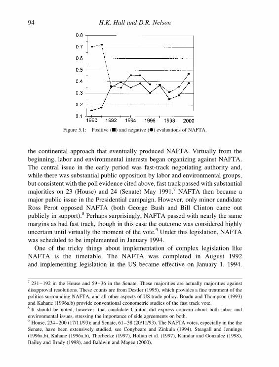
the continental approach that eventually produced NAFTA. Virtually from the

beginning, labor and environmental interests began organizing against NAFTA.

The central issue in the early period was fast-track negotiating authority and,

while there was substantial public opposition by labor and environmental groups,

but consistent with the poll evidence cited above, fast track passed with substantial

majorities on 23 (House) and 24 (Senate) May 1991.7 NAFTA then became a

major public issue in the Presidential campaign. However, only minor candidate

Ross Perot opposed NAFTA (both George Bush and Bill Clinton came out

publicly in support).8 Perhaps surprisingly, NAFTA passed with nearly the same

margins as had fast track, though in this case the outcome was considered highly

uncertain until virtually the moment of the vote.9 Under this legislation, NAFTA

was scheduled to be implemented in January 1994.

One of the tricky things about implementation of complex legislation like

NAFTA is the timetable. The NAFTA was completed in August 1992

and implementing legislation in the US became effective on January 1, 1994.

Figure 5.1: Positive (B) and negative (X) evaluations of NAFTA.

7 231–192 in the House and 59–36 in the Senate. These majorities are actually majorities against

disapproval resolutions. These counts are from Destler (1995), which provides a fine treatment of the

politics surrounding NAFTA, and all other aspects of US trade policy. Boadu and Thompson (1993)

and Kahane (1996a,b) provide conventional econometric studies of the fast track vote.8 It should be noted, however, that candidate Clinton did express concern about both labor and

environmental issues, stressing the importance of side agreements on both.9 House, 234–200 (17/11/93); and Senate, 61–38 (20/11/93). The NAFTA votes, especially in the the

Senate, have been extensively studied, see Conybeare and Zinkula (1994), Steagall and Jennings

(1996a,b), Kahane (1996a,b), Thorbecke (1997), Holian et al. (1997), Kamdar and Gonzalez (1998),

Bailey and Brady (1998), and Baldwin and Magee (2000).


It incorporated and expanded most of the provisions of the CFTA that was halfway

into its 10-year phase-in period. While the agreement eliminated tariffs on many

goods immediately (over half of US imports and nearly a third of exports with

Mexico), it began the phasing-out of remaining tariffs over a 15-year period. Most

of the anticipated effects of the agreement on the US economy, however, were

through provisions covering a broad range of nontariff barriers, foreign direct

investment, intellectual property rights, trade in services, and a number of other

trade facilitating agreements (on customs administration, product standards,

antitrust, and telecommunications). Many of these provisions were also to be

phased-in over time. There were also two well-publicized side agreements on

environmental and labor cooperation.

Prior to NAFTA implementation, the average US tariff rate on imports from

Mexico was only around 3% and half by value already entered the US duty-free.

By 1996, about three-fourths of US imports from Mexico were duty free with an

average tariff of around 2.5% on the remainder (including sectors such as motor

vehicles and motor vehicle parts, apparel and textiles, and fresh vegetables). The

average tariff rate in Mexico on US goods started at around 10% prior to NAFTA

and in 1996 was down to approximately 3% on NAFTA goods. Also, the share of

US exports entering Mexico duty free increased from roughly one-third to two-

thirds by 1996.

Most provisions on nontariff barriers were still being implemented in 1996. In

particular, prohibitions, quantitative restrictions, and import licensing require-

ments by Mexico were still being phased-out with the use of tariff-rate quotas.

Additionally, implementation was not yet complete in a number of key industries.

For example, Mexico is phasing-out trade and investment restrictions on

Figure 5.2: Ratio of positive to negative evaluations.


automobiles over 10 years—including a slow reduction in local content

requirements from 36% to only 34% in the first 5 years. Additionally, the US is

phasing-out quotas on textiles and apparel made with foreign material over a 10-

year period and both countries are phasing out nontariff barriers on agriculture

(import licenses in Mexico and quota shares in the US) over 10 or 15 years using

tariff-rate quotas. Implementation by Mexico is also not complete in the

telecommunications, transportation services, and financial services industries. The

provisions related to foreign direct investment, intellectual property rights, trade

in services, customs administration, and product standards were fully in effect

by 1996.10

Complicating an assessment of the impact of NAFTA on the US was the fact

that theWTOAgreements entered into effect only 1 year later and addressed many

of the same issues. In general, the WTO Agreements were broader than the

NAFTA and went farther in sectors such as agriculture and telecommunication

services, but fell short with respect to foreign direct investment and government

procurement. Notable overlap includes areas such as sanitary measures, textile

and clothing, antidumping, safeguards, intellectual property rights, and dispute

settlement. The WTO Agreements also lowered US tariffs by nearly a third and

began a 5-year phase-in period of tariff reductions on most products, with a 10-

year phase-in period on sensitive sectors (such as textiles). Mexico did not reduce

their MFN tariffs as a result of the WTO Agreements and, instead, merely bound

their rates generally at 35%. In fact, in response to the peso crisis, Mexico raised

MFN tariffs on 502 consumer goods in 1995 from an average of 20–35%. US

exports to Mexico under the NAFTA were exempt from these tariff increases.

Thus, the major political event in the period 1991–1992 was the fast-track vote.

The passage of the legislation, and thus the final legal form of NAFTA was not

determined until the end of 1993, with “implementation” occurring in 1994.11 It

would be hard to argue that the sizable shift in opinion occurring between 1991

and 1993 was a function of the sort of shifts in political fundamentals that might be

taken to account for changed policy preferences in standard political economy

models. While the institutional environment had not changed significantly, it is

entirely possible that a change in economic conditions induced the change in

public trade policy preferences. We know from previous research on the correlates

of trade policy that trade balance and general macroeconomic conditions are

10 For a much more detailed discussion of the status of NAFTA implementation in 1996, see Chapter 2

of The Impact of the North American Free Trade Agreement on the US Economy and Industries: A

Three-Year Review, US International Trade Commission, publication 3045.11 With reference to Levy’s (1998) paper we simply note that (1) opinion shifts well before this date;

and (2) actual implementation occurs much later (i.e., many of the most significant changes in US and

Mexican law were scheduled to occur only with lags of up to 15 years).


associated with changes in trade policy demands. Figure 5.3A shows the balance

on goods and services (1980–1999), where 1991 is the last year of a multi-year

improvement in the trade balance and where 1992 and 1993 show positive

performance by historical standards. By contrast, the large deteriorations in 1998

and 1999 do not appear to be particularly associated with changed evaluations.

Similarly, Figure 5.3B shows the (possibly more relevant) merchandise trade

balance with Mexico, where we see 1991 and 1992 are years of improving trade

balances and, again, the large deterioration from 1994 to 1995 is not associated

with changed evaluations. Aggregate economic indicators, shown in Figure 5.4,

are equally unsupportive of an economic fundamentals story.12 The period of

Figure 5.3: (A) US balance on trade in goods and services. (B) US–Mexico merchandise trade

balance.

12 It should also be recalled that this is the period of realignment of the US dollar from a period of very

large overvaluation. It will be recalled that the dollar began accelerating in late 1980 or early 1981,

reaching its peak in February 1985, and ultimately returning to something like an equilibrium level in

late 1987 or early 1988. The essential fact would seem to be that 1991 is at the end of a period of

exchange rate instability, while 1996 is in a relatively stable period.


strongest support coincideswith a period of low (even negative in 1991) growth and

high unemployment, while the periods of weaker support are characterized by

stronger growth performance and lower unemployment. The picture that emerges

from these data is clear: standard theoretical and empirical models of trade policy

preference/behavior would have predicted greater activism in 1990–1993 than in

the latter half of the decade. Interestingly, this suggestion is supported by the data in

Figure 5.5, which shows the number of Title VII (anti-dumping and countervailing

duty) petitions initiated per year. Activity in the administered protection

mechanisms, of which the Title VII mechanism is the most prominent, is well

known to be a major indicator of protectionist activity. That figure shows a

relatively smoothly rising trend in filings consistent with a period of deteriorating

economic performance, and a drop in 1995 to a lower annual level offilings.13Thus,

as we asserted at the outset of this section, it would be difficult to attribute to

changed institutional ormaterial conditions the shift in public attitudes with respect

to NAFTA.

Figure 5.4: Aggregate economic indicators: (P) unemp; (X) drlGDP.

13 The spikes in 1992 and 1997 are associated with massive steel industry filings that are determined

institutionally (i.e., as a part of the steel industry’s strategy relative to the mechanism) and are not in

any obvious way associated with Mexico, Canada, or NAFTA.

Although, using annual data (1980–1999 and 1990–1999) there are too few data points for

convincing analysis, simple regression of Title VII petitions on unemployment and trade balance

suggests that both of these play a role in explaining filing behavior (with unemployment playing the

larger role). Carrying out the same analysis using positive responses, negative responses, or their ratio

yields no significant results at all.


5.2. POLICY COMPLEXITY, SOCIAL LEARNING

AND FOOTLOOSE PREFERENCES

As economists/political-economists, the conclusion of Section 5.1 leaves us in

an awkward position. All positive political economy models operate by

assuming that the policy preferences of individuals are derived in some

relatively straightforward way from the effect of policy (and policy changes) on

material well-being. But we have just displayed a case where policy preferences

changed, and changed dramatically, with no relevant change in material or

institutional conditions. In this section we argue that the complexity of NAFTA

makes determining the effects of implementation difficult. It is under precisely

such conditions that we might expect agents to condition their behavior on the

actions of others, not for strategic reasons, but because those who have already

taken actions might reasonably be expected to possess knowledge one does not

possess. This attempt to learn from the behavior of others is called social

learning.

From the point of view of the citizen, or policy-maker, trade policy is extremely

complex. Trade policy rarely comes in the form of a single, discrete act of

protection.14 Instead, trade policy is embedded in legislative acts made up of

complicated bundles of changes in the law regulating trade that even experts have

a hard time evaluating. NAFTA is a very interesting example. NAFTA itself is

Figure 5.5: Title VII petitions initiated.

14 Even in the days of the classic tariff system—say, 1870 to 1932—the political action revolved

around tariff acts with hundreds of line items. In addition, as research on 19th century voting suggests,

the social meaning of the tariff was highly variable across local electorates.


a document of over 300 pages (not including the national tariff schedules and

various other lists—with these the text runs over 2000 pages) covering trade in

goods, technical barriers to trade, government procurement, investment, services,

intellectual property, and the administrative and institutional conventions needed

for implementation; the agreement on environmental cooperation is another 20

pages; as is the agreement on labor cooperation; all of these need to be

implemented with specific national regulations in all three signatory countries.

Some of these regulations will affect trade in goods, others will affect trade in

factors of production; some will liberalize this trade, others will restrict it. In

addition, while NAFTA officially became law in 1994, as we saw above, full

implementation will not occur in sensitive sectors for periods of 10–25 years. In

this environment even trade economists might be expected to have fairly diffuse

priors with respect to NAFTA’s aggregate and distributional effects.15

Clearly, in the case of NAFTA, some form of “learning” had occurred, since

expressed evaluations had shifted fairly dramatically. What is completely unclear

is what triggered this reassessment. There was virtually no NAFTA-specific

information and the aggregate facts of the economy suggest the sort of

environment in which trade is usually viewed relatively benignly. This would

seem to be a virtually archetypal example of footloose preferences. Given the

weakened domestic political institutions supporting trade liberalization in the US,

and the concomitant likelihood of increased prominence for trade as a public

political issue, such footlooseness of trade preferences could play a significant role

in the future politics of trade.16 As proponents of liberal trading relations, it

behooves us to seek an understanding of such preferences.

While there may have been no change in the material or policy environment,

the period from 1991 to 1996 (and especially 1991–1993) was characterized by

an extraordinary amount of public discussion about NAFTA. It was the first

instance of highly public trade politics since the heyday of the classic tariff

system and, as such, it may tell us something about the politics of trade in years

to come. NAFTA was in the news, it was dinner table and cocktail party

conversation among non-economists, every politician had (and had to have) a

public opinion (sometimes different from their private opinion). Perhaps most

15 For the purposes of this chapter we abstract from the central importance to the US of locking in

Mexican economic reforms. This is consistent with nearly all of the political-economy research on free

trade areas in general, and NAFTA in particular. Though see the important series of papers by Ethier

(1998a–c, 1999, 2002).16 The events surrounding the WTO meeting in Seattle (30 November 1999), illustrate this point even

more clearly than does the politics of NAFTA. Nelson (1989) provides a discussion of the role and

transformation of US trade policy institutions for the support of trade liberalism. Nelson (1995)

discusses the collapse of those institutions in the early 1970s.


importantly, NAFTA was a major issue in the 1992 presidential election. Trade

economists approached minor celebrity status, and the unanimity with which

trade economists concluded that NAFTA was economically insignificant for the

US was truly stunning. With similar unanimity we heaped well-earned scorn on

dishonest claims about the “giant sucking sound”.17 But note that the timing is

important. NAFTA really takes off as public issue only when candidate Ross

Perot decided to focus on it, and this focus really comes after the change in

public evaluations. While both Patrick Buchanan and Perot were critical in 1991

and 1992, it is only in 1993 (especially with the publication of Perot’s book in

September and the Gore–Perot debate in November) that there was wide

discussion of the issue. Where economists appear to have been successful in

convincing Congress that NAFTA’s economic effects would be small, the public

was clearly confused and worried (with “undecided” responses rising rapidly in

1991 and 1992).

Clearly, high uncertainty and learning play a major role in the NAFTA case.

However, at least if we believe that the effects of NAFTA were likely to be small

(and probably positive), as we claimed at the time, this is a peculiar kind of

“learning”. That is, instead of converging on the “true” facts of the matter, the

public moved in the opposite direction. One useful way of approaching this

phenomenon is to consider it as an example of herd behavior. Herding occurs

whenever agents focus on a single behavior, with particular reference to cases in

which there are multiple plausible candidate behaviors. The phenomenon of herd

behavior is common enough that it has been used as the basis for a wide variety of

economic analyses based on such things as demand interdependence (Leibenstein,

1950; Schelling, 1978; Becker, 1991) and network externalities (Dybvig and

Spatt, 1983; David, 1985; Farrell and Saloner, 1985; Katz and Shapiro, 1985). An

alternative explanation in terms of information cascades has recently been

presented by Bikhchandani, Hirshleifer, and Welch (BHW, 1992), and further

developed in a number of later papers.18

In an environment where individuals can learn about the environment from both

private information and the behavior of others, an information cascade occurs

when agents ignore their private information and follow the information implied

by the behavior of others. Where the behavior of others is not perfectly

informative with respect to their private information, an information cascade

effectively traps socially useful information, thus permitting socially suboptimal

17 It is probably useful, given the recent vogue among trade economists for attacking free trade areas, to

recall that during the NAFTA debate support for NAFTA was seen as a litmus test of one’s status as a

serious economist.18 See Bikhchandani et al. (1998) and Nelson (1998) for surveys.


outcomes. Thus, the essential elements of the information cascade model are

coarse public signals and private signals of bounded accuracy. Without the first

assumption, the law of large numbers suggests that, with a sufficiently large

number of observations, the true state of the world is revealed (almost surely). In

most information cascade models this assumption takes the form that agents

observe the actions of other agents but not their signals, and that the actions are

imperfectly informative with respect to signals. Without the second assumption,

individuals might receive fully informative signals, allowing them to take actions

that would break the cascade. In addition, BHW (1992) make a number of

additional assumptions that permit a very simple expository model.

Consider the NAFTA case. Suppose that we start from an equilibrium and,

thus, from a cascade involving all citizens. Specifically, suppose we start from a

situation in which people have essentially no beliefs at all about NAFTA, and

possibly have a weakly held belief that trade liberalization (whether NAFTA or

multilateral) would have a negative effect on the economic interests of the US.19

That is, we assume that citizens as a whole believe that trade liberalization is

harmful, but this support of increased liberalization is highly conditional and

subject to large shifts. Now recall that in the run up to the fast-track vote,

virtually all respectable economists and the political leadership of both parties

argued very publicly that, essentially, NAFTA was no big deal economically for

the US, but that it was important politically (by being important economically

for Mexico). The result, as we have already noted, was strong public support for

NAFTA. However, the public had not learned that liberal trade was good, if by

“learned” we mean “identified the true state of the world”, but had simply shifted

to another weakly held prior. With the campaigns in 1992 and the debate over

NAFTA itself in 1993, the opposition forces began to receive considerable

greater visibility and, even though there was no change in the material

environment, people shifted their evaluations. Furthermore, once NAFTA was

passed by Congress, economists in general (and trade economists in particular)

not only lost interest in NAFTA, but began to argue that maybe NAFTA was not

such a great idea after all. It is not really relevant that the free trade

fundamentalist critique of NAFTA was that it distracted political attention from

19 Both assumptions here strike us as plausible approximations for the purposes of this example. What

poll data exist with respect to trade policy generally strongly suggests that a considerable majority

believes further liberalization will be harmful to the US economy—though there is little evidence of

support for general increases in protection (though support for sectoral increases is often strong)—see

Scheve and Slaughter (2001). Furthermore, there is very little evidence that citizens make much of a

distinction between preferential and multilateral liberalization. This makes sense. The difference in

complexity, from the point of view of a citizen, between NAFTA and, say, a GATT agreement, is

trivial.


broader trade liberalization. The public listens for the conclusion, not

the argument—especially when the argument is, at best, arcane.20 The result,

in the face of continued aggressive public relations against NAFTA, as we have

already noted, is that public opinion shifted back to opposition to NAFTA.

5.3. AN ILLUSTRATIVE MODEL

This section sets up a very simple political economy model of individual citizen

preferences for or against the NAFTA under uncertainty over the impact of the

agreement. Preferences over the trade agreement depend on two factors: an

economic effect; and a political effect. The latter reflects the claim that NAFTA

would help lock-in liberal political and economic reforms in Mexico. We will

assume that this effect is certain, but has a relatively small weight in citizen

welfare. The first reflects concerns with the economic effects of NAFTA on US

labor. Poll data seem to suggest that negative evaluations of NAFTA were

highly correlated with a perception of high labor adjustment costs in the US. If

Mexico is economically small, we suppose that there are no significant

adjustment costs; but if Mexico is large there will be significant adjustment

costs. Furthermore, if Mexico is large, the adjustment costs are taken to

outweigh the benefits of locking in Mexican reform. We will assume that these

preferences are common and reflected in a common evaluation function

VðE;PÞ U vðEðSÞÞ2 P; where E and P reflect the economic and political

factors, S denotes the economic size of Mexico, and vð·Þ is the value of

protecting displaced factors from adjustment costs, so a positive value of Vð·Þ

implies a preference for rejecting NAFTA.21

20 Abstracting from details of trade creation and trade diversion, which are characterized by complexity

considerations of the sort central to this chapter, it is notable that virtually all of the arguments against

regionalism, whatever their validity, are arguments that only an economist would love. Unlike the

simple models used to illustrate powerful, but difficult, notions of comparative advantage and gains

from trade, which are based on assumptions that isolate the key causal relation generating gains from

trade, the political economy arguments used to argue against free trade areas are based on assumptions

that seem unrelated to the core processes involved. Their purpose seems more to be to stiffen the spine

of the profession in its support of multilateralism than to persuade citizens or their representatives.21 That is we are assuming that citizens have a very simple form of sociotropic preferences (Kinder and

Kiewiet, 1981; Mutz and Mondak, 1997), i.e., they evaluate policies in terms of the way policy affects

community welfare. We simplify by assuming that the relevant community is the nation as a whole, and

that the evaluation of community welfare is unaffected by individual preference. These latter two

assumptions are generally false. We can prove the existence of cascades in more standard political

economy models, but the additional analytical freight does not produce any additional insight relative

to the central point of this chapter: footlooseness of policy preferences.


We now assume that Mexico’s size is uncertain. Each agent, therefore, faces

a decision under uncertainty of whether or not to reject the trade agreement

depending upon whether he/she expects it to be welfare improving. Specifically,

we will assume that each citizen observes a conditionally iid signal si ¼ {L; S}and that si . 0:5 if the true value of Mexico’s size is L and 12 si if the true value

is S: In addition to the private signal, citizens take their action in a known order

and each citizen observes the action (but not the signal) of all agents that precede

them in this order. Thus, after the first citizen decides whether or not to reject

NAFTA, all later deciders have two sources of information: one public, and one

private. It is common knowledge that all agents are Bayesian rational. If we adopt

BHW’s normalization of vðHÞ ¼ 1; vðLÞ ¼ 0; P ¼ 12; and letting gi be the

posterior probability that Mexico is large: E½vi� ¼ gi £ 1þ ð12 giÞ £ 0 ¼ gi; andVi . 0 if gi .

12: Finally, BHW adopt the tie-breaking convention that a citizen

that is indifferent between rejecting and accepting NAFTA chooses to accept.

This model is now identical to that of BHW’s “specific model” (BHW, 1992,

pp. 996–999).

The logic of cascades is straightforward in this model. Suppose that the

first citizen observes s1 ¼ L: She has no additional information, so V1 ¼

12 12. 0 and she rejects NAFTA. For citizen 2 there are two possibilities:

s2 ¼ L and citizen 2 rejects; or s2 ¼ S; so citizen 2 computes E½v2� ¼12; V2 ¼

0; and by the tie-breaking rule accepts. Citizen 3 is in one of three cases: both

the previous citizens reject NAFTA, so citizen 3 rejects independently of her

private signal; both previous citizens accepted, so citizen 3 accepts

independently of her private signal; or 1 and 2 split, in which case 3 is in

the same situation as 1—i.e., her private signal determines her action. Either

of the first two cases is a cascade: all later citizens ignore their private signals

and adopt the same action of those preceding them. In this simple framework

it is easy to see that: cascades occur with probability 1; cascades occur more

quickly the further is s from 0.5; and good cascades occur more often the

further is s from 0.5. With reasonably high uncertainty, s not terribly far

from 0.5 (as we have argued may have been the case with NAFTA), but with

a large number of citizens, everyone knows that they are in a cascade almost

surely. This is the opening wedge for BHW’s other key result that: (1) once

an informational cascade has begun, individuals still value public information

and (2) a small amount of public information can reverse a cascade. That is,

even a strong informational cascade rejecting NAFTA can be suddenly

reversed into an equally strong cascade supporting the agreement. The key

result here is their result (3) “the release of a small amount of public

information can shatter a long-lasting cascade, where a ‘small amount’ refers


to a signal less informative than the private signal of a single individual”

(BHW, 1992, p. 1005).22

5.4. CONCLUSION: ON ECONOMISTS AS PARTICIPANTS

IN THE POLITICS OF TRADE POLICY

It is important to be clear that, while the class of models considered here is

positive, they are not predictive over the domain of final political-economic

outcomes. These models do not avoid, in fact they rest on (or, more accurately,

provide a formal representation of) the fact that, with appropriately chosen

priors, we can reproduce virtually any final outcome.23 Thus, any predictions of

these models with respect to final outcomes are vacuous. Nonetheless, we hope

that this chapter suggests that ignorance and learning in a social context are

issues of first-rate importance, both as empirical phenomena and as potential

determinants of trade policy outcomes. Furthermore, there are, we think, several

implications of these models (and of ignorance/learning more generally) for us

as policy analysts. We consider two: one with respect to evaluating the

predictive content of our positive models; and the second with respect to the role

of economists in the public discourse over trade policy.

There is no substitute for basing predictive political-economy models on

political and economic fundamentals. We have good reason to expect such

fundamentals to play a central role in determining trade policy, andwe have equally

good reason to predict the direction of the effects. However, if learning effects also

play a, largely unpredictable, role, we also need to expect prediction errors that are

occasionally large. That is, the right kind of ignorance can yield wildly different

outcomes from those predicted by models. An excellent example, away from the

trade policy focus of this chapter, is the poor performance of macro political-

economy models in the 1992 Bush–Clinton election (Haynes and Stone, 1994).

While the data seem to show recovery of the economy, and thus success for the

22 BHW (1992) develop their analysis in a somewhat more general informational environment

involving a sequence of possible signals and a more careful formalism. More importantly, it would be

straightforward to extend their analysis to the case of preference heterogeneity, as generated, for

example, in a standard endogenous tariff model, under full information about citizen types. In that case,

while actions (e.g., accept, reject, abstain) will vary, so there need not be complete herding, there will

still be good and bad cascades with strictly positive probability. More interesting possibilities emerge

with type heterogeneity and uncertainty about types. Smith and Sørensen (2000) develop this case in

detail. This is an important topic for future research, but beyond the needs of the simple point made in

this chapter.23 It is the reproduction of outcomes that is most worrying in social scientific analysis. Thin predictions

(unless strictly unfalsifiable) will not last, but compelling post-dictions (“stylized facts”) can sustain

empirically weak theoretical analyses for long periods.


incumbent, there was widespread perception that the economy was still in an

economic crisis (“It’s the economy stupid”). The result, as they say, is history.

As noted in the introduction and suggested by the discussion of the NAFTA case,

one of the most interesting implications of learning models with information

cascades as a prediction is the suggestion of a major role for policy analysts. Some

of the recent attempts to justify an active policy role for economists turn on difficult

philosophical issues of freedom of choice that seem rather removed from the actual

practice of participation by economists in the public policy discourse. The advice

on how and whom to advise that emerges from this kind of argument seems of

limited use.24 The problem seems to emerge from taking our models seriously

where we should not. We have just argued that these models serve a very useful

positive purpose in understanding and predicting public policy. However, when we

abstract from complexity and uncertainty in the interest of building parsimonious

models, we have abstracted from the most obvious warrant for an active advisory

role. When agents, whether citizens or policy-makers, are highly uncertain about

the workings of the economy (i.e., most of the time), expert advice can have a

substantial effect on final outcomes via precisely the channels identified in learning

models.25 It makes perfectly good sense for citizens and politicians to listen to, and

even to seek out, the advice of economists because that advice is better informed

thanmuch of the policy advice that is given during a political process—though note

that this need not be even vaguely perfect information. A public signal of strong

agreement among economists, especially when supported by compelling evidence,

during a political process can have the effect of a public information release in the

models discussed above. Even if policy-makers, or citizens, believe that this

information is less informative than any individual privately observed signal, such a

public release can have the effect of reopening the public discussion and

dramatically shifting the structure of governmental or public opinion.26

24 This is the entering wedge for Dixit’s (1997) comment on O’Flaherty and Bhagwati (1997).25 Just as trade and political economy models abstract from informational issues to focus on the causal

forces of most immediate interest, learning models of the sort developed in this chapter abstract from a

variety of complexities to highlight the effects of ignorance and learning in a social context. In

particular, these models abstract from the important, and complementary, forces that make advisors

participants (in a game theoretic sense) in the political process. Dixit (1997) provides a very nice

sketch, with appropriate references, of models which highlight the role of advice giving in a strategic

environment with asymmetric information.26 Although we are presumably better informed, as we noted above, economists are at least as prone to

being trapped in cascades as any other rational agents engaged in learning about the world, possibly

more so. Because economists have very similar understandings of the workings of the economy—due

to strong socialization—we may behave more like the agents in the BHWmodels than any other group.

Smith and Sørensen (2000) find much more complex aggregate behavior characterizing groups with

heterogeneous preferences than in groups with homogeneous preferences.


It seems to us that a focus on this non-strategic, informational role of economic

advice has useful implications. To the extent that the warrant for advice-giving is

uncertainty, as much about the working of the economy as about simple facts, it

seems particularly fruitless to give advice based on the presumption that those

receiving it are well-trained economists.27We need to convince our auditors that a

consensus on fundamental issues related to, say, trade policy, exists, and we need

to do so in ways that are clear to relatively engaged, relatively intelligent

non-economists. This clearly means that complicated arguments, requiring many

closely argued steps, and knowledge of economic theory, are likely to be

unsuccessful. However, as Matthew Slaughter (1999) argues, while outright lies

may be successful in the short-run (e.g., “NAFTA will create thousands of jobs”),

sooner-or-later they are likely to backfire. The most successful of our public

representatives—e.g., Milton Friedman, Alan Blinder, Paul Krugman—seem to

identify simple but compelling metaphors, which are mixed with a small number

of striking facts, to argue for a single clear policy point. Finally, it should be noted

that, if social learning does not produce knowledge of the intertemporally sturdy

type, but rather of the type suggested by informational cascade models, we need to

be prepared to stay engaged in the public discourse beyond the passage of any

particular piece of legislation.

ACKNOWLEDGEMENTS

The authors would like to thank participants at the 1999 ASSA meetings, New

York, NY and the 25th Anniversary Meeting of the International Economic Study

Group, September 9–11, 2000, Isle of Thorns, Sussex. In particular, we are

grateful to comments from Alan Winters and Devashish Mitra.

REFERENCES

Bailey, M. and Brady, D. (1998). Heterogeniety and representation: the senate and free


Baldwin, R. and Magee, C. (2000). Is trade policy for sale? Congressional voting on recent

trade bills. Public Choice, 105, 79–101.

Becker, G. (1991). A note on restaurant pricing and other examples of social influence on

price. Journal of Political Economy, 99, 1109–1116.

27 While admirable, the attempt to transform citizens and policy-makers into economists is almost

certainly doomed to failure.


Bikhchandani, S., Hirshleifer, D. andWelch, I. (1992). A theory of fads, fashion, custom, and

cultural change as informational cascades. Journal of Political Economy, 100, 992–1026.

Bikhchandani, S., Hirshleifer, D. and Welch, I. (1998). Learning from the behavior of

others: conformity, fads, and informational cascades. Journal of Economic Perspectives,

12, 151–170.

Boadu, F. and Thompson, M. (1993). The political economy of the U.S.–Mexico free trade

agreement: analysis of the congressional fast track vote. Journal of Agricultural and

Applied Economics, 25, 27–35.

Conybeare, J. and Zinkula, M. (1994). Who voted against the NAFTA.World Economy, 19,

1–12.

David, P. (1985). Clio and the economics of QWERTY. American Economic Review. 75,

332–337.

Destler, I. M. (1995). American Trade Politics, 3rd edn., Washington, DC: Institute for

International Economics.

Dixit, A. (1997). Economists as advisers to politicians and society. Economics and Politics,

9, 225–230.

Dybvig, P. and Spatt, C. (1983). Adoption externalities as public goods. Journal of Public

Economics, 20, 231–247.

Ethier, W. (1998). The international commercial system. Essays in International Finance,

#210.

Ethier, W. (1998). The new regionalism. Economic Journal, 108, 1149–1161.

Ethier, W. (1998). Regionalism in a multilateral world. Journal of Political Economy, 106,

1214–1245.

Ethier, W. (1999). “Multilateral roads to regionalism,” in International Trade Policy and

the Pacific Rim, J. Piggot and A. Woodland (eds.), London: Macmillan, 131–152.

Ethier, W. (2002). Unilateralism in a multilateral world. Economic Journal, 112, 266–292.

Farell, J. and Saloner, C. (1985). Standardization, compatibility, and innovation. Rand

Journal of Economics, 16, 70–83.

Haynes, S. and Stone, J. (1994). Why did economic models falsely predict a Bush landslide

in 1992. Contemporary Economic Policy, 12, 123–130.

Holian, D., Krebs, T. and Walsh, M. (1997). Constituency opinion, Ross Perot, and roll-call

behavior in the U.S. house: the case of the NAFTA. Legislative Studies Quarterly, 22,

369–392.

Kahane, L. (1996). Congressional voting patterns on NAFTA: an empirical analysis.

American Journal of Economics and Sociology, 55, 395–409.

Kahane, L. (1996). Senate voting patterns on the 1991 extension of the fast track trade

procedures: prelude to NAFTA. Public Choice, 87, 35–53.

Kamdar, N. and Gonzalez, J. (1998). An empirical analysis of the U.S. senate vote on

NAFTA and GATT. International Advances in Economic Research, 4, 105–114.

Katz, M. and Shapiro, C. (1985). Network externalities, competition and compatibility.

American Economic Review, 75, 424–440.

Kinder, D. and Kiewiet, D. (1981). Sociotropic politics: the American case. British Journal

of Politics, 11, 129–161.


Leibenstein, H. (1950). Bandwagon, Snob and Veblen effects in the theory of consumer

demand. Quarterly Journal of Economics, 64, 183–207.

Levy, P. (1998). “Learning from trade agreements,” MS, Department of Economics, Yale

University.

Lustig, N. (1998). Mexico: The Remaking of an Economy, 2nd edn., Washington, DC:

Brookings.

Mayer, F. (1998). The Science and Art of Policy Analysis, New York: Columbia University

Press.

Mutz, D. and Mondak, J. (1997). Dimensions of sociotropic behavior: group-based

judgements of fairness and well-being. American Journal of Political Science, 41,

284–308.

Nelson, D. (1989). The domestic political preconditions of US trade policy: liberal structure

and protectionist dynamics. Journal of Public Policy, 9, 83–108.

Nelson, D. (1995). “Political economy of protection for the US automobile industry,” in

Political Economy of American Trade Policy, A. Krueger (ed.), Chicago: University of

Chicago Press, 133–191.

Nelson, D. (1998). “Footloose policy preferences and trade policy: the role of non-strategic

social learning and information cascades,” MS, Murphy Institute of Political Economy.

O’Flaherty, B. and Bhagwati, J. (1997). Will free trade with political science put normative

economists out of work? Economics and Politics, 9, 207–219.

Pastor, M. and Wise, C. (1994). The origins and sustainability of Mexico’s free trade

policy. International Organization, 48, 459–489.

Schelling, T. (1978). Micromotives and Macrobehavior, New York: Norton.

Scheve, K. and Slaughter, M. (2001). Globalization and the Perceptions of American

Workers, Washington, DC: Institute for International Economics.

Slaughter, M. (1999). Globalisation and wages: a tale of two perspectives.World Economy,

22, 609–629.

Smith, L. and Sørensen, P. (2000). Pathological outcomes of observational learning.

Econometrica, 68, 371–398.

Steagall, J. and Jennings, K. (1996). Unions, PAC contributions, and the NAFTA vote.

Journal of Labor Research, 17, 515–521.

Steagall, J. and Jennings, K. (1996). Unions and NAFTAs legislative passage:

confrontation and cover. Labor Studies Journal, 21, 61–79.

Ten Kate, A. (1992). Trade liberalization and economic stabilization in Mexico: lessons of

experience. World Development, 20, 659–672.

Thorbecke, W. (1997). Explaining house voting on the north American free trade

agreement. Public Choice, 92, 231–242.

Tornell, A. and Esquivel, G. (1997). “The political economy of Mexico’s entry into

NAFTA,” in Regionalism versus Multilateral Trade Arrangements, T. Ito and A.

Krueger (eds.), Chicago: University of Chicago Press, 25–55.

Weiss, J. (1992). Trade liberalization in mexico in the 1980s: concepts, measures and short-

run effects. Weltwirtschaftliches Archives, 128, 711–726.


PART II

Making of Trade Policy:

Empirical Analysis

CHAPTER 6

Interest and Ideology in the 1988

Omnibus Trade Act: A Bayesian

Multivariate Probit Analysis

ALOK K. BOHARA,a KISHORE GAWANDE,b,*

aDepartment of Economics, MSC05 3060, 1, University of New Mexico,

Albuquerque, NM 87131-0001, USAbGeorge Bush School of Government and Public Service, Texas A&M University,

4220 TAMU, College Station, TX 77843-4220, USA

Abstract

The landmark 1988 Omnibus Trade and Competitiveness Act marked an

important change in US trade policy. Using new Bayesian methodology that

facilitates model comparisons in a multivariate probit model, we study whether

ideology or interest determined congressional voting. We find that Senate voting

was driven equally by economic factors, mainly constituent interests, and political

factors, mainly party. House voting, on the other hand is largely determined by

party and ideology. We also find a common underlying factor not accounted by

the set of explanatory variables. We call this factor “trade ideology”, as distinct

from conventional liberal-conservative ideology.

Keywords: Multivariate probit, congressional voting, interest, ideology

JEL classifications: D72, C35, F13



…I can note that the Administration will resist the following: First that

we would impose a general surcharge…Second, we oppose sector-

specific protection, such as establishing import quotas for individual

producers…Third, we oppose mandatory retaliation.And, finally, Mr.

Chairman, it comes as no surprise, I know, that we will oppose limits on

Presidential discretion.

Treasury Secretary James Baker, at Senate hearings before the Finance

Committee, 100th Congress, first session, February 19, 1987.

I see a dramatic change in the policy of this Administration, much more

aggressive trade policy and tougher trade policy……The fact is that trade

is the handmaiden of all other policy considerations of the U.S.

Government and it will continue to be so unless we have some limits on

the President’s discretion.…We need a trade policy that our trading

partners can predict and I maintain that requires limits on the President’s

discretion not to act.

Chairman of the Finance Committee, Senator Lloyd Bentsen, at Senate hearings

before the Finance Committee, 100th Congress, first session, April 2, 1987.

In considering any amendment to Section 301, I hope youwill ask one key

question: Will this amendment help or hurt the ability of U.S. negotiators

to pry open a foreign market to U.S. exports? It really comes down to this

issue: Is Section 301 an import-relief law, or is it a negotiating

tool?……What you have to have is a credible threat of retaliation…

US Trade Representative General Counsel Alan Holmer, at Senate hearings

before the Finance Committee, 100th Congress, first session, March 17, 1987.

6.1. INTRODUCTION

The literature on the determinants of voting behavior has a long and rich history in

political science and economics. Vigorous debate persists about the importance of

“ideology” versus “interest” in explaining voting behavior (Kau and Rubin, 1979;

Kalt and Zupan, 1984; Peltzman, 1984). Adherents of ideology (Poole and

Rosenthal, 1997; Kalt and Zupan, 1984) emphasize party and liberal-conservative

ideology as the main determinant of politicians’ voting behavior, while

proponents of interest emphasize lobbying and constituency interests as

A.K. Bohara and K. Gawande114

fundamental determinants of congressional voting (Kau et al., 1982; Peltzman,

1984, 1985; Irwin, 1994). The recent literature presumes that the two chambers

respond fundamentally differently. Bailey and Brady (1998) focus on Senate

voting and constituency interests. Levitt and Snyder (1995) show that in the House

parties influence policy outcomes that favorably redistribute income to their

districts. Adler and Lapinski (1997) show that since committees are composed of

members representing districts that have a demonstrated need for policy benefits

under the jurisdiction of those committees, constituency interests matter to House

voting. We visit the ideology versus interest debate in the setting of a landmark

legislation, the 1988 Omnibus Trade and Competitiveness Act.

The Act changed the nature of US trade policy from its previously free-trade

orientation. Although the change in US trade policy had been in evidence since

the 1979 Trade Act, the 1988 Act cemented the change. It made US trade policy

more aggressive and activist, and provided a basis for more strategic trade

policy. It was enacted during the term of a President strongly in favor of free

trade, and hence required forceful legislation in Congress. It lessened the ability

of the President to make discretionary decisions without consulting Congress, a

factor that contributed to previous free-trade stance of the US Enacted during a

time of weak world institutions in trade, the Super 301 provisions of the 1988

Act allowed greater unilateralism. This has disturbed political economists from

the free-trade persuasion (e.g., Bhagwati and Patrick, 1990) while giving

legitimacy to the activist strategic school (e.g., Krugman, 1986). Roll call votes

taken during legislation of the 1988 Act spanned a range of issues, providing for

a rich setting for examining the relative importance of interest versus ideology.

Tosini and Tower (1987) were among the first to study congressional voting on

trade bills. They considered voting on the protectionist 1985 Textile Bill, focusing

on variables that measured economic interest behind voting. Their study found

that senators and representatives responded to a variety of influences while voting

on the bill, including campaign contributions, union power, unemployment in

their constituencies, and the economic importance of the textile industry in their

constituencies. Many of the variables used by Tosini and Tower have informed the

economic variables used in this study.

We methodologically extend the study of roll call voting data by employing a

multivariate probit model (MVP). Any analysis of roll call votes on connected

issues, many occurring within days of each other, must come to grips with the fact

that there will be jointness across the votes. The correct methodology is, therefore,

a multivariate approach. That is, each congressman’s votes on a set of bills are

correctly modeled as a draw from a multivariate distribution. Merely conditioning

on a set of exogenous variables in a single equation analysis misses crucial

information present in the error correlations, leading to inefficient estimation.

Interest and Ideology in the 1988 Omnibus Trade Act 115

Our finding of statistical significance and large magnitudes on the error

correlations bears this out.

Methodologically, the chapter showcases an important new statistical

technology due to Chib and Greenberg (1998), namely the Markov Chain

Monte Carlo (MCMC) method. This method is useful whenever high-dimensional

integration is required in estimation, which is true of Bayesian analysis in general

(and classical analysis of the MVP). With a reasonably high dimension, say,

greater than two, the estimation of the MVP model by traditional methods is

cumbersome and becomes increasingly inaccurate as the number of dimensions

increases. The MCMC method also allows model comparisons with ease. Non-

nested model comparisons of models emphasizing ideological factors versus

models emphasizing interest are featured here. We believe it to be an innovation in

the legislative studies literature.

In Section 6.2 the historical context of the Omnibus bill is described. It is

followed by a description of the methodology. The set of hypotheses central to the

empirical work and the data used to examine them are then described in Sections

6.3–6.5. The empirical results are analyzed in Sections 6.6 and 6.7. Section 6.8

concludes via conventional significance tests as well as formal model comparisons.

6.2. BACKGROUND: THE TRADE OMNIBUS ACT

Table 6.1 presents a summary of the features of the Omnibus Act and the route the

bill took to become law. Table 6.2 details the roll calls. The genesis of the 1988

Act lay in a strategic and relatively protectionist bill that was passed by a large

majority in the House in 1986 (HR 4800). However, the Senate refused to consider

it since support for the bill fell far short of the two-thirds majority required to

override a certain presidential veto. The 99th Congress saw a shift in power in the

Senate, with 54 Democrats and 46 Republicans, and the stage was set for activist

trade legislation. The House Ways and Means Committee, with primary

jurisdiction over trade matters, authored bill HR3 in 1987 under the shrewd

chairmanship of Dan Rostenkowski (D-IL). It was marked up by four other

committees making for an Omnibus bill.1 The most controversial part of HR3 was

the Gephardt amendment, named after Rep. Gephardt (D-MO), who would later in

the year run for the Presidential nomination. The Gephardt amendment would

make it mandatory for the President to retaliate against partners with “excess”

trade surpluses vis-a-vis the US (i.e., if their exports totaled 175% of imports)

1 Energy and Commerce added strategic amendments to promote exports in high-tech US goods;

Foreign Affairs added amendments furthering US exports, and on relaxing export controls; banking

added strategic amendments on exchange rates and third world debt.


Table 6.1: Evolution of the Omnibus bill: house, senate, conference, and final versions.

Features of the House bill Features of the Senate bill

H.R.3

(Introduced

in Ways

and Means)

(1) Presidential negotiating authority: approval

of fast track for 5 years

(2) Transfer of authority over Section 301

(unfair trade practices) cases and retaliation to

USTR—a lower level of official making this

decisions rather than the president. Also, authority

over Section 201 (escape clause), and 337

(intellectual property rights)

transfers from president to USTR

(3) Section 301: mandatory action against agreement

violation but otherwise up to president’s discretion.

“Special 301” allowed self-initiation on an annual

basis of 301 cases against priority foreign

countries who failed to protect intellectual

property rights

(4) Gephardt bill: USTR required to retaliate

against unfair trade practices; mandatory

action against foreign countries to reduce

their bilateral trade imbalance by 10%

per year until 1991

(5) AD/CVD: extended to high-tech and

agricultural goods from its traditional focus

on steel and other heavy industries

(6) Bryant amendment: disclosure

of foreign ownership in a US

business to be reported to SEC

S1420 (Introduced

in Finance)

(1) Presidential negotiating authority:

possibility of withdrawal by Congress

of president’s access to fast track

(2) Section 201: shift of earlier focus

on protection to prevent injury to

protection to assist industry to adjust

to import competition; mandatory

funding of such adjustment. Less

ability for president to deny ITC

decision for protection; but set higher

standard for industry in order to file

under 201. Expansion of Trade

Adjustment Assistance

(3) Section 301: severely reduced

president’s discretion not to act in

301 cases. Expansion of scope of

practices actionable under 301. Amend

Section 301 to include “mandatory but

not compulsory” retaliation against

unjustifiable or discriminatory foreign

(e.g., Japan) practices

(4) Other issues: telecommunications

trade opportunities; intellectual

property rights protection; access

to foreign technologies; auctioned quotas

(continued)

InterestandIdeologyin

the1988OmnibusTradeAct

117

Table 6.1: (continued)

Features of the House bill Features of the Senate bill

Michel (R-IL) substitute for H.R. 3 (#78)

passed on 4/30/87, 290–137. It excluded

Gephardt (but adopted Rostenkowski’s

alternative which was similar to Gephardt

except for “surplus reduction” measures),

Bryant, and “Buy America”

provision. Else same as above

S1420 passed (7/21/87), 71-27 (#208) with

addition of 34 (out of 160 proposed)

amendments. “Super 301” introduced:

relation to target consistently protectionist

countries. Amended S1420 close

to original version above

Features of the Conference Bill

Rostenkowski (Chair, House Ways and Means) started by proposing to drop most protectionist sections, and Bentsen (Chair, Senate Finance)

reciprocated the sentiment. The bill adopted in conference, still called H.R.3 was a less protectionist version of the above bills, but contained their

activist and strategic elements. It dropped Gephardt but included a labor-backed plant closing provision which required employers to give 60 days

notice of plant closings or layoffs. It passed 312–107 on 4/21/88 in the House (#66), and 63–36 on 4/27/88 in the Senate (#110), and was sent to

President Reagan

Final Omnibus bill

The bill was vetoed by President Reagan on 5/24/8 8, citing the plant closing provision. The House vote on the same day (#150) overrode the veto, but

the Senate vote of 61–37 (#169) on 6/8/88 failed to override. A new bill in the House, H.R. 4848, close to the vetoed bill but without the plant closing

provision, was voted in 376–45 by the House (#231) on 7/13/88, and 85–11 (#288) by the Senate on 8/3/88. It was signed into law on 7/23/88. The

plant closing provision made its way through the Senate and House as a separate bill (S2527) and became law in August 1988

Abbreviations: USTR, US Trade representative; AD/CVD, Antidumping Duty/Countervailing Duty; TAA, Trade Adjustment Assistance; SEC,

Securities and Exchange Commission. Sections 201 and 301 refer to same Sections of the Trade Act of 1974.

A.K.Bohara

andK.Gawande

118

if this excess was due to unfair trade practices.2The amendment passed with amere

four-vote margin on the House floor, but would be dropped in conference. It was

anticipated that Reagan would veto the bill since, other than being an activist bill

even without the Gephardt amendment, it sought to curb discretion of the executive

in granting or denying protection. That discretion had been used by Reagan to

reverse the decision of the International Trade Commission (ITC), the independent

bipartisan body that made determinations under Sections 201, 301 and 337 of the

US Trade Act. The ITC had found for the petitioners seeking protection.

In the Senate, the Finance Committee with primary jurisdiction over trade

matters, led by Sen. Bentsen (D-TX), proposed a Senate bill similar in content to

HR3. While it was an activist bill, it was less protectionist. It contained no

Gephardt-like provisions. However, it contained a labor-backed provision on plant

closing (requiring employers in large firms to give 60 days prior notice to any

plant closings or layoffs) that would be the basis for Reagan’s veto of the Omnibus

bill. The Senate failed to override the veto, and this provision was dropped to

ensure passage of the 1988 Omnibus Trade and Competitiveness Act. The plant

closing provision succeeded separately and became law in 1988. Though the

Omnibus bill was an activist “fair trade” bill, its authors Rostenkowski and

Bentsen pushed to drop explicitly protectionist provisions from the bill. They

foresaw the need for substantial support from moderate Republicans. Hence, the

protectionist Textile bill was not packaged into the Omnibus bill, Gephardt’s

provision was dropped, as was the plant closings provision after the veto.3

6.3. ANALYSIS OF THE MULTIVARIATE PROBIT MODEL

The econometric methodology employed in this chapter is described here at an

intuitive level. For full technical details we refer the reader to Chib and

Greenberg (1998) and Chib (1995). The Bayesian method of estimating the MVP,

due to Chib and Greenberg (1998), is employed in this chapter because it is

appropriate for the study of multiple roll call voting on related issues (Table 6.2).

The method facilitates formal model comparisons, which is a major focus of this

study. While it allows the incorporation of prior information formally into the

estimation, in this study we use only weak priors, which are easily dominated

2 The genesis to the Gephardt amendment lay in an import surcharge bill during 1986 authored by

Rostenkowski, Gephardt and Senator Bentsen, all key players in the Omnibus bill. But later

Rostenkowski and Bentsen distanced themselves from it and it became Gephardt’s amendment.3 There may have been implicit agreements among the architects of the Omnibus bill and these other

bills about reciprocal support. To maintain focus, we do not formally test for logrolling here, leaving

this open for future work.


Table 6.2: Roll call votes analyzed in the multivariate probit models.

House bills Senate bills

Bill # Short description Date Vote Bill # Short description Date Vote

72 Gephardt(D-MO). Mandatory retaliation

to lower trade surplus

4/29/87 218–214 158 Bentsen (D-TX). Against

Specter’s motion for private

right of action to sue

against unfair trade

6/25/87 69–27

77 Michel (R-IL). Drop Gephardt, Wylie,

and Bryant (see Table 6.4) amendments

4/29/87 156–268 175 Bradley (D-NJ)/Packwood(R-OR).

Against requiring President to

keep oil imports below 50%

of consumption

7/1/87 55–41

78 Omnibus Bill, House version. Like

Michel’s version (77). Activist,

Strategic. See Table 6.4

4/30/87 290–137 178 Packwood (R-OR). Allow

President discretion over

ITC cases on account of

national interest

7/7/87 41–55

426 Michel’s (R-IL) motion to instruct

House conferees to concede

Gephardt amendment

11/10/87 175–239 179 Domenici (R-NM).

Expand definition of

unfair trade practices

7/8/87 71–28

66 Omnibus Bill passage, Conference version.

Gephardt dropped. Plant closing included

4/21/88 312–107 208 Omnibus Bill passage,

Senate version. See Table 6.4

7/21/87 71–27

231 Final Omnibus Bill Passage: After

dropping plant closing and Gephardt

7/13/88 376–45 110 Omnibus Bill passage, Conference

version. See Table 6.4

4/27/88 63–36

285 Bensten (D-TX). Defend the

provision in the Bill to transfer

authority from President to USTR

8/3/88 69–26

Notes: full descriptions of roll calls available from authors. Other roll calls taken on the Omnibus bill but not included in the analysis: #150(S),

#77(H), #206(S), #169(S), #114(H), #197(H), #319(H) #132(S), #250(S), #190(S), #229(H) #267(H), #341(H), #426 (1988) (H), #225 (S), 288 (S),

329 (S), 332 (S).

A.K.Bohara

andK.Gawande

120

by data evidence. Hence, for all practical purposes the results are based on the

data, not prior information, so as to service the widest readership. Weak priors

also adequately represent our prior beliefs about the determinants of voting on the

Omnibus Act.

Consider the J-variate probit model where Yij is a random variable denoting a

binary 0=1 response on the ith observation on the jth variate. Let yi ¼ ðyi1;…;yiJÞ0;

1 # i # n; be the J-variate realization on the ith observation. The MVP model is

conditioned on the parameters b : k £ 1; and S : k £ k and a set of explanatory

variables Xi; as follows:

yi ¼ Xibþ ei; ð1Þ

where the data yi : j £ 1 as described above, Xi is a ðJ £ kÞ matrix of explanatory

variables given as diagðxi10;…; xiJ

0Þ; where xij : kj £ 1 is the set of kj explanatory

variables in the jth equation (hence k ¼P

Jj¼1 kjÞ; b : k £ 1 is the vectors of

coefficients on the explanatory variables, and ei : J £ 1 is the (correlated) vector

of residuals with zero mean and correlation matrix S : J £ J: In Bayesian analysisof the model, b and S are assigned a prior distribution (here these prior

distributions represent ignorance, so inferences are from the data, not priors).

Inference proceeds with the analysis of the posterior distribution, which combines

the prior probability density function with the data likelihood.

The estimation of the posterior mean of the parameters (used to make

inferences) and the posterior ordinate at the posterior means (used to perform

model comparisons) are performed via a powerful computational method

involving MCMC sampling. Estimation by MCMC methods has been used

effectively in the Bayesian analysis of several econometric models (e.g., Chib and

Greenberg, 1996). In applications of MCMC methods an overriding feature is

that the joint density (“posterior density” in Bayesian applications, or “data

likelihood” in non-Bayesian applications) is not analytically well defined. But it

can be broken down into the product of conditional densities that are analytically

well defined, from which synthetic samples may be taken. The Gibbs sampler

derives its utility from the fact that generating sequences of samples from the

conditional distributions upon updating the conditioning parameters, results in a

sample that is actually generated from the joint density itself. That sample can be

used to compute the posterior mean or maximum likelihood estimate, and also

the ordinate of the posterior density or value of the likelihood function. Chib and

Greenberg (1998) provide explicit conditional distributions and sampling methods

to generate samples from the joint multivariate probit density, from which b and Sare estimated. Using Chib’s (1995) method the sample is also used to perform

formal comparisons of competing models of legislative behavior.


6.4. THEORY AND MEASUREMENT

This study is concerned with the empirical investigation of three issues in

legislative behavior:

† determinants of voting behavior on redistributive issues, specifically trade

legislation,

† relative importance of ideology and interest, and

† whether and why determinants of voting may vary across chambers.

Several studies we reference below, which provide the basis for the explanatory

variables in our econometric model, present illuminating though diverse answers

to the first question. However, most empirical studies of voting are content with

testing hypotheses against no specific alternatives, and are silent on the second

issue. We are aware of no studies that formally weigh their own hypotheses

against well-specified alternatives, which is a distinguishing feature of this study.

On the third question, most studies to date are again silent. We do not pretend to

provide a full, or even adequate, answer to this third question. Since the analysis of

a closely related set of votes across both chambers is possible, we are presented

with a natural experiment that allows us to shed light on possible inter-chamber

heterogeneity. Our hope is that theoretical explanations able to formalize what we

find empirically will be forthcoming. The remainder of this section is devoted to

describing our empirical models, which are founded on a set of recent theoretical

and empirical studies. Baldwin (1986) and Conybeare (1991) model the electoral

market for protection as the equilibrium outcome of demand and supply factors. In

this model, existing protection leads to a demand for more protection. Since

protection has income effects (more protection raises incomes), and is a normal

good, districts/states with greater protection will desire more of it. On the supply

side, a politician is likely to vote for greater protection the lower is her opportunity

cost of doing so. A politician is also likely to vote for greater protection depending

on her institutional capacity to supply protection. In our setting Democrats

possessed the larger institutional capacity to vote for trade activism.

In the present setting, a reduced form equation predicting voting on, say, issues

that are for activism or protectionism, we would expect to find a positive sign on

previous protection, a positive sign on variables decreasing in the opportunity cost

of providing protection, and negative sign on party (the variable PARTY being

measured as a binary variable: 1 if Republican, and 0 if Democrat). To measure

existing protection we employ a tariff measure (TARIFF), and a nontariff barrier

measure (NTB). To measure the opportunity cost of providing protection we

employ the net-exports-to-shipment-ratio (NETEXP) and the unemployment rate


(UNEMP). Low values of NETEXP indicate comparative disadvantage and hence

lower opportunity cost of voting for protection, while higher values of UNEMP (in

a time of economic boom) indicate industries in distress and hence lower

opportunity cost of voting for protection. NETEXP is thus expected to have a

negative (positive) sign on votes for protection (free trade). On votes for

protection, a positive sign is expected on UNEMP.

Irwin’s (1994) study of British voting on free trade in 1906 demonstrates the

importance of sectoral employment in the pattern of voting. We similarly measure

constituency interests by employment shares in food processing (FOOD), which

cross-industry studies of protection have shown to be a pro-protectionist sector.4

Bailey and Brady (1998) and Bailey (2001) theorize that the relationship

between constituency characteristics and roll call voting varies with party. This

hypothesis about inter-party heterogeneity is based on the premise that there are

systematic differences across parties in how electoral coalitions are built. They

find evidence in favor of inter-party heterogeneity from 1993–1994 Senate voting

on key issues related to NAFTA and GATT. We incorporate the Bailey–Brady

hypothesis by interacting TARIFF, NTB, and NETEXP with PARTY, where

PARTY equals 1 for Republicans and 0 for Democrats.5 Significance of the

interaction terms are evidence of heterogeneity in how a politician’s party

qualifies her response to constituency interests.

Irwin and Kroszner (1999) study the Republican conversion to trade

liberalization during the 1940s after the Republican enactment of the Smoot–

Hawley tariffs of the 1930s. Their theory favors interest over ideology. Interacting

party with exports, they find that sensitivity to exporting industries in their

constituencies, rather than any shift in ideology, was the main factor responsible

for the Republican “conversion” to the Democratic free-trade initiative.

Empirically, their finding reinforces Baily and Brady’s finding that inter-party

heterogeneity was a huge factor in how Republicans converted. Curiously, party

heterogeneity in the Baily–Brady sense brought the parties closer in the final vote.

In our case, the role of Democrats is reversed—their agenda is, if not protectionist,

an activist one. Hence, we expect to find exactly the reverse of what Irwin and

4 In a previous version of the chapter, other sectors such as textile and apparel (APPAREL), autos,

aerospace, and other transport equipment (TRANSPORT), resource-based manufactures, for example,

refined petroleum, wood, and furniture (RESOURCE), and other manufactures including machinery,

electronic goods, scientific instruments, primary metals, and iron and steel (OTHERMNF) were used

but they were significant neither statistically nor in magnitude. They were dropped in the analysis

reported here.5 Naturally, all constituency interest variables are candidates for interactions with party. We chose

TARIFF, NTB, and NETEXP as candidates since these are most closely associated with trade

orientation of constituents.


Kroszner find, if their theory about which Republicans convert first is to be

confirmed in our setting—Republicans favoring export interests would be the last

to convert to any protectionist trade legislation that was essentially a Democratic

agenda. A negative sign on the interaction term NETEXP £ PARTY on

protectionist issues and a positive sign on free-trade or export-promoting issues

would be inline with the Irwin–Kroszner mechanism in our setting.

A large literature has developed around the question of whether party measures

interest or ideology in empirical studies. This follows the general finding of the

dominating influence of party in studies of legislative behavior. A consensus, by

no means unanimous, is emerging in the direction of parties as evolving

institutions based on interest. The theory put forth by Cox and McCubbins (1993)

has gained wide acceptance. Cox and McCubbins model party as a mechanism

designed to solve the collective dilemmas of rational but unorganized reelection-

seeking legislators. These collective dilemmas lead to situations that are worse for

all legislators than outcomes attainable by organized action—individual

optimization by self-interested politicians achieve a lower level of success than

if they optimized and their party had a majority. The primary method of solving

collective dilemmas is the creation of leadership posts through which the

organization operates effectively. Hence “parties are invented, structured and

restructured in order to solve a variety of collective dilemmas that legislators

face”. Party, in this view, is an interest-based mechanism designed to resolve the

collective action problem of self-interested actors.6 Parties are groups of

politicians who sometimes act together to achieve collective goals but whose

cooperation is limited by their conflicting preferences. A party that sustains a large

majority in Congress over a long period is able to fashion a portfolio of programs

that favors its constituency. Since activist trade legislation in the House during

the 1970s and 1980s was expected to result in redistributive policies, we feel the

Cox–McCubbins view of parties as interest-based coalitions provide the

appropriate explanation of why the Democratic party was able to form a forceful

coalition during the 1988 Omnibus Act.

The Cox–McCubbins view has been reinforced in recent empirical studies.

Levitt and Snyder (1995) show that parties play a significant role in determining

geographic distribution of domestic federal expenditures. Schickler and Rich

(1997) show that even though there may be dissent within a party, when pitted

6 An alternate view, which was generally accepted before the Cox–McCubbins view became popular,

is the “strong party” model in which parties are effectively treated as unitary actors that maximize some

mix of policy and reelection goals. But that theory was unable to explain how or why a party that

sustains a large majority in Congress over a long period is able to fashion a portfolio of programs that

favors its constituency.


against another party, members of the former vote cohesively. McGillivray

(1997) affirmatively tests the hypothesis that the level of party discipline is an

important factor is determining the characteristics of regions which receive

protection. We expect PARTY to enter with a negative sign on votes for

protectionism and activism, certainly on the various versions of the full Bill. We

also expect the interaction of party with constituency interest to be important in

differentiating the Democratic and Republican response.

A counterpoint to the view of party as an interest-based mechanism, is one of

voting based on pure ideology espoused by Poole and Rosenthal (1997). Their

factor-analytic study of historical roll call voting over a hundred years is

interpreted by the authors to lead to the singular conclusion that general liberal-

conservative ideology was the driving force behind voting over the century.

Intuitively, they find one, or at most two, significant factors underlying historical

roll call voting. These factors map into a pattern that split clearly along party lines

and regions, leading Poole and Rosenthal to conclude that the party-region split

represents clear ideological divisions that form the basis of yea and nay voting in

recent history.

Ideology is measured here, as in many studies of voting, by raw ADA scores

(ADA) for House and Senate members.7 We perform a sensitivity analysis of the

effect of including three other measures of ideology (summarized at the end of

Section 6.6). Poole and Rosenthal’s mapping of factors into party and region space

make a compelling case to consider region, after adequately controlling for

interest, as measures of ideology. We indicate three regions with the eponymous

variables NORTHEAST, WEST and SOUTH.

The Poole–Rosenthal interpretation has been challenged by Heckman and

Snyder (1997), who use a simpler factor-analytic method (which the authors show

is more appropriate than the Poole–Rosenthal methodology) to show that six or

more factors are required to fully explain historical voting over the period

considered by Poole and Rosenthal. They put forth the hypothesis that issue-

specific ideology, as opposed to general liberal-conservative ideology, is

responsible for the greater number of dimensions. Issue-specific ideology is not

observable, making it difficult to explicitly assess the Heckman–Snyder claim.

The MVP method provides a natural way of investigating the presence of any

latent factor during legislation of the Omnibus bill via estimates of the error

covariance matrix. Evidence of an issue-specific ideology, here “trade ideology”,

would be reflected in significant error covariances.

7 ADA scores are average ratings by Americans for Democratic Action (ADA) of Congressmen for

1985–1986. The ADA rating is the percentage of times a congressman voted for the ADA position on a

selected sample of 20 issues.


Nollen andQuinn (1994) have performed the only other analysis of voting on this

bill. Their study covers voting onmore than 30 roll calls taken during the legislation

of the Omnibus bill is designed to uncover the coalitions and motivations behind

voting on free trade issues, fair trade issues, strategic trade issues, and

protectionism. Of importance is their use of direct measures of special interest

based on the pressure group model of Olson (1965), which we also employ. They

are the proportion of all PAC contributions accounted by labor PACs

(PACLABOR), domestic corporate PACs (PACCORP), and domestic PACs with

the largest exports or overseas sales (PACINTL).

In sum, the explanatory variables in the voting equations, described fully in

Table 6.3, may be grouped as follows: regional dummies (NORTHEAST,

SOUTH, WEST); committee membership (HTRADESUB, WAYSMEANS,

INTLDEVSUB, SENTRADESUB, FOREIGNREL); special interest pressure

(PACCORP, PACINTL, PACLABOR); constituency interest (UNEMP, FOO-

DEMP, NETEXP); economic interest (TARIFF, NTB); party membership

(PARTY); and inter-party heterogeneity (NETEXP £ PARTY, TARIFF £

PARTY, NTB £ PARTY); and ideology (ADA).

6.5. DATA

Data on roll call votes taken during legislation of the Omnibus bill are from

Congressional Quarterly’s online database. Votes of 99 senators and 425

representatives are used in the study.8 Data on political variables and PAC

contributions are taken fromNollen and Quinn (1994), to which we refer the reader

for data sources and construction. We are grateful to the authors for sharing their

data. Table 6.3 describes the variables, and Tables 6.4 and 6.5 present descriptive

statistics.

Regional dummies for three regions, NORTHEAST, SOUTH, WEST, cover

75% of the Senate and House samples. Committee membership are indicated in

three relevant House committees (HTRADESUB, WAYSMEANS, INTLDEV-

SUB) comprising 10% of reps., and two relevant Senate committees (SENTRA-

DESUB, FOREIGNREL) comprising 36% of senators.

8 Votes other than “Y” (Yea) and “N” (Nay) were treated as follows. “?” (did not vote) were imputed as

1 (Y) or 0 (N), respectively, if the mean on the vote was greater than 0.5 or less, conditioning on party;

“ þ ” were converted to 1 (Y) id “ 2 ” to 0 (N); “#” were converted to 1 (Y) and “X” to 0 (N); “S”

(Speaker did not vote) was deleted; “I” (not allowed to vote for part of 87–88) were deleted. The MVP

method requires the same number of observations for each roll call vote in the model. We included as

many observations as possible via simple imputations. The number of observations for which

imputations were made is generally less than 2% of the sample for any roll call.


Table 6.3: Variable definitions.

Variable Description

NORTHEAST 1 if congressman from Northeast, 0

otherwise

SOUTH 1 if congressman from South, 0

otherwise

WEST 1 if congressman from West, 0

otherwise

HTRADESUB 1 if Repp. on Intl. Economic

Policy and Trade Subcommittee of the

House Foreign Affairs Committee

WAYSMEANS 1 if Repp. on Trade subcommittee

of the House Ways and Means

committee 0 otherwise

INTLDEVSUB 1 if Repp. on International Development,

Finance, Trade, and Monetary Policy subcommittee

of the House Banking, Finance, and

Urban Affairs Committee, 0 otherwise

STRADESUB 1 if Senator on Intl. Trade

subcommittee of the Senate Finance committee,

0 otherwise

FOREIGNREL 1 if Senator on Foreign Relations

Committee, 0 otherwise

PARTY 1 if Republican, 0 if Democrat

ADA Liberalism measure rating based on voting

record by Americans for Democratic Action:

0 (very conservative) to 100 (very

liberal)

PACCORP Contributions from domestic corporate PACs as

% of total PAC contributions (domestic

corporations do not include

international corporations defined

for PACINTL)

PACINTL Contributions from international corporate PACs as

% of total PAC contributions

(international corporations

comprise either the 100 largest US

corporations in terms of foreign sales

or the 50 largest US exporters

during any year during 1982–1988

PACLABOR Contributions from labor union PACs as

% of total PAC contributions

UNEMP Unemployed persons as % of the labor force in 1986

FOODEMP Percent of manufacturing labor force in

food processing manufacturing

(continued)


Table 6.3: (continued)

Variable Description

TARIFF Tariff rate as of 1983 (data

section for construction)

NTB Nontariff barrier coverage ratio as of

1983 (see data section for construction)

NETEXT NetExports ¼ Exports 2 Imports, as of 1986 (see data

section for construction)

Notes: data are across states for senators and congressional districts for Representatives. Data (except

FOODEMP, TARIFF, NTB, NETEXP) taken from Nollen and Quinn (1994). See their Appendix A for

more details.

Table 6.4: Descriptive statistics: explanatory variables.

Variable Senate data (N 5 99) House data (N 5 425)

Mean SD Min Max Mean SD Min Max

NORTHEAST 0.222 0.418 0 1 0.247 0.432 0 1

SOUTH 0.263 0.442 0 1 0.292 0.455 0 1

WEST 0.263 0.442 0 1 0.198 0.399 0 1

HTRADESUB – – – – 0.031 0.172 0 1

WAYSMEANS – – – – 0.033 0.179 0 1

INTLDEVSUB – – – – 0.035 0.185 0 1

STRADESUB 0.172 0.379 0 1 – – – –

FOREIGNREL 0.192 0.396 0 1 – – – –

PARTY 0.455 0.500 0 1 0.412 0.492 0 1

ADA 0.467 0.341 0 1 0.478 0.349 0 1

PACCORP 0.294 0.133 0 0.640 0.233 0.115 0 0.672

PACINTL 0.295 0.175 0 0.667 0.259 0.178 0 1.068

PACLABOR 0.144 0.138 0 0.454 0.223 0.205 0 0.838

UNEMP 0.697 0.223 0.280 1.310 0.678 0.263 0.100 1.800

FOODEMP 0.127 0.110 0 0.567 0.129 0.157 0 1

TARIFF 0.538 0.131 0.323 0.916 0.561 0.235 0 1.951

NTB 0.214 0.067 0.123 0.458 0.188 0.110 0 0.596

NETEXP 20.644 0.268 21.538 20.082 20.539 0.444 23.61 0.408

PARTY £ TARIFF 0.232 20.267 0 0.878 0.216 0.290 0 1.952

PARTY £ NTB – – – – 0.072 0.108 0 0.576

PARTY £ NETEXP 20.293 0.376 21.538 0 20.201 0.384 23.61 0.409

Notes: variables are scaled to have similar size for purposes of estimation: PACINTL is scaled by 10,

PACLAB and PACCORP by 100, UNEMP by 10, ADA by 100, TARIFF by 10, NTB by 10. The

descriptive statistics here and the results in subsequent tables reflect this scaling. Mean: sample mean,

SD: sample standard deviation, Min: sample minimum, Max: sample maximum.


The ideology versus interest debate is at the heart of the chapter. Ideology is

measured by raw ADA scores for House and Senate members. A sensitivity analysis

also includes three competing measures of ideology: a measure from Levitt (1996)

that purges ADA scores of interest, and two separate ratings based on voting on

economic matters constructed, respectively, by the US Chamber of Commerce and

National Journal (Cohen and Schneider, 1989). Nollen and Quinn’s (1994)measures

of special interest include the proportion of all PAC contributions accounted by labor

PACs (PACLABOR), domestic corporate PACs (PACCORP), and domestic

corporate PACs with the largest exports or overseas sales (PACINTL).9

The unemployment rate (UNEMP) is from Nollen and Quinn. The share of the

Food processing sector in manufacturing employment (FOODEMP) is con-

structed as follows. The state level data on employment were straightforwardly

obtained from the geographic area series of the 1987 Census of manufacturing.

The mapping in Congressional District Atlas (Department of Commerce, 1984)

was used to concord the county-level Census data into districts.10

Data on ad valorem tariffs (TARIFF), nontariff barrier coverage ratios (NTB),

and net-exports-to-shipments ratio (NETEXP) are unavailable across states and

districts, and are estimated using Conybeare’s method (also used by Bailey and

Brady (1998)) from their national averages. First, US averages for exports ðXÞ;

Table 6.5: Descriptive statistics: roll calls.

Senate data House data

Roll call (Year, #) Mean SD Roll call (year, #) Mean SD

1987, 158 0.73 0.45 1987, 72 0.50 0.50

1987, 175 0.56 0.50 1987, 77 0.37 0.48

1987, 178 0.42 0.50 1987, 78 0.67 0.47

1987, 179 0.72 0.44 1987, 426 0.41 0.49

1987, 208 0.73 0.44 1988, 66 0.74 0.44

1988, 110 0.64 0.48 1988, 231 0.89 0.31

1988, 285 0.73 0.45

SD ¼ Sample standard deviation.

9 Nollen and Quinn (1994, Appendix A) report that data for senators are from 1983–1988 and for reps.

from 1985–1986. In 1987–1988 there were 1873 corporate PACs and 135 International PACs in

1987–1988. International PACs are not counted as domestic corporate PACs in computing PACCORP.

The total of the three PAC variables sums, on average, to around 60% of the total PAC money received

by senators and reps.10 If the county-to-district mapping was one-to-many, the employment data were proportioned equally;

if the mapping was many-to-one, then the county data were added up. The employment shares variables

were then computed.


imports ðMÞ; shipments ðSÞ and value added (V) all for 1986, and TARIFF and

NTB as of 1983,11 are computed for the 20 two-digit SIC industries. The two-digit

values are then weighted down to a state/district level value, using as weights the

proportions of the state/district’s manufacturing value added accounted by the 20

industries. For example, the tariff rate on imports into state or district i is given as

TARIFFi ¼P20

j¼1 wijTARIFFj; where wij ¼ Vij=Vi:The variables NTBi; ðX=SÞi; ðM=SÞi; are similarly constructed as weighted

averages of their two-digit values using wij as weights. The net export to shipment

ratio (NETEXP) for state/district i is then computed as ðX=SÞi 2 ðM=SÞi:

6.6. EMPIRICAL ANALYSIS

6.6.1. Substantive issues of focus

Linear dependencies among roll call votes may make it difficult to estimate the

MVP model. For this reason, MVP models of House and Senate voting include at

most three roll calls at a time. The choice of which roll calls to include is based on

two issues common toHouse and Senate voting and a third issue exclusive to Senate

voting.12 The first and most important set of issues concerned voting on the full

Omnibus bill itself. There were four House bills at different stages of the process

(#78—House passage, #66—adoption of conference bill, #150—veto override,

#231—final passage), and four Senate bills (#208—Senate passage, #110—

adoption of conference bill, #16—veto override, #288—final passage).13

The second set of issues was related to a push for protectionism. Action on the

House floor centered around the controversial Gephardt amendment (#72), which

explicitly targeted Japan, Taiwan, and Hong Kong. It barely passed the House,

overcame two efforts at getting rid of it (#77, #426), but was dropped in conference.

11 X;M; S; V are from the 1986 Annual Survey of Manufactures. TARIFF, NTB are described in Trefler

(1993).12 The bills are chosen to represent different clusterings of issues. Otherwise the multivariate analysis

of very similar bills breaks down due to linear dependency among them. Narratives from weekly issues

of Congressional Quarterly (CQ), examination of the nature of the bill (protectionist, free, curtailment of

Presidential powers, strategic), voting splits, breakdown of the vote by party, and simple correlations are

inputs into deciding how the bills cluster.13 There were no explicit votes taken on many important characteristics that were bundled into the

Omnibus bill. The Super 301 provisions under Section 301, which granted Congress the power to

undertake unilateral action against unfair trade practices by any partner, was one such key

characteristic. It was considered by free-traders as the single most damaging aspect of the Act (see, e.g.,

Bhagwati and Patrick, 1990). Since no roll call votes were taken on 301, the only analysis on this issue

is from the voting on the passage of successive versions of the bill itself.


On the Senate floor a set of bills relating to protectionism sought to amend Section

201 dealing with import injury cases (#158, #179, #206), with some winning and

others losing. The third set of issues, debated in the Senate, concerned discretionary

powers of the executive which they had used to overturn decisions by the ITC

(#175, #178, #285). Championed by Bentsen (D-TX), Chair of the Senate Finance

Committee, those issues also concerned the transfer of authority over protection

cases from the President to the US Trade Representative (USTR). The USTR was

perceived as being more independent of state agencies under control of the

executive, who could interfere with trade cases.

6.6.2. Analysis of MVP estimates from HOUSE voting

Estimates from MVP models analyzing House voting is presented in Table 6.6.14

Model 1 estimates the trivariate model of voting on Gephardt’s (D) amendment to

the House Omnibus bill (#72), Michel’s (R) somewhat less protectionist substitute

(#77) for the House Omnibus bill, and passage of the House Omnibus bill (#78).

Model 2 jointly analyzes the Michel (R) motion to drop Gephardt (#426) from the

conference bill, and voting on the conference bill (#66) itself. Model 3 jointly

analyzes passage of the House version (#78), Conference version (#66), and the

final version (#231) signed into law. Each of the three MVP models includes a

version of the full Omnibus bill for the reason that the important roll call votes were

amendments to the Omnibus bill under consideration, and helped shape the bill.

The coefficient estimates fromModel 1 testifies to the persistence of the ideology

versus interest debate. The evidence across voting on the Gephardt (D) amendment

(#72), the Michel (R) substitute (#77), and the House version of the Omnibus bill

(#78) show that while the ADA and regions (if one subscribes to the Poole–

Rosenthal view of region as representing ideological tradition) are significant deter-

minant of voting on protectionism, special interests (in particular PACLABOR),

constituency interests (UNEMP, FOODEMPL), and other measures of interest

(TARIFF, NTB) are each statistically significant across the three roll calls.15

14 We are indebted to Sid Chib for providing us the code for the MVPmodel estimation. After a bum-in

of 500 discarded samples, a sample of 5000 was used to compute the estimates. The estimates are

comparable to single-equation probit results, but there are differences in statistical significance and

magnitude due to systems estimation and the inclusion of S in the MVPmodel. Computational note: on

a P4 machine, a trivariate House model such as Model 1 in Table 6.6 took 45 min and a trivariate

Senate model took 15 min to run.15 Asterisked estimates are interpreted as being statistically significant. * implies that 2 . ltl $ 1 and

** implies ltl . 2:A rationale for using this criterion to denote statistical significance is that (in a linear

regression setting) only if a variable has a coefficient with ltl $ 1 will its exclusion lower the model’s

adjusted R2 and its inclusion raise it (e.g., Greene, 1993, p. 193).


Table 6.6: Estimates from MVP models of House voting.

Variable Model 1 Protectionism 1 RepublicanBill 1 House Bill

Model 2 GephardtRedux 1 Conference Bill

Model 3 House 1 Conference 1 FinalBill

# 72 (P) # 77 (F) # 78 (P) # 426 (F) # 66 (P) # 78 (P) # 66 (A/P) # 231 (A)

CONSTANT 2 1.820* 2.874* 2 1.284* 1.835** 0.058 2 1.323* 0.585 20.114

NORTHEAST 0.315* 2 1.852** 0.113 20.389* 0.506* 0.237 0.670* 0.444*

SOUTH 20.669** 20.074 20.303 0.265 0.286* 20.252 0.373* 1.207**WEST 2 1.657** 0.705* 2 2.325** 0.925** 20.302* 2 1.797** 20.325 20.105

HTRADESUB 0.115 20.091 1.094* 20.326 1.489** 0.764* 1.713** 0.599

WAYSMEANS 20.861* 0.989* 0.722* 20.308 2 2.476** 0.530* 21.936** 20.124

INTLDEVSUB 0.672* 1.047 0.157 0.737* 20.617* 0.029 20.685* 0.466

PARTY 2 1.543** 4.013** 2 1.453* 2.078** 20.089 2 1.433* 20.527 0.043

ADA 0.577* 2 3.119** 2.769** 2 1.841** 3.357** 2.485** 3.116** 1.866**PACCORP 1.982* 2 6.393** 0.779 21.929* 22.570* 1.440* 22.162* 22.056*

PACINTL 20.304 0.422 20.229 20.255 20.023 20.428 20.335** 0.363

PACLABOR 3.190** 2 2.358* 0.721 2 3.124** 2 1.945* 0.888 2 2.293 2 1.445*UNEMP 1.256** 20.941* 0.869* 21.198** 0.722* 0.678* 0.443* 1.132**FOODEMPL 22.225** 6.776** 2 3.820** 2.833** 0.899 2 2.998** 1.115* 0.793

A.K.Bohara

andK.Gawande

132

TARIFF 0.692* 2 3.840* 2.268* 0.064 0.704 2.703* 0.957 1.856*NTB 2.964** 2 7.342** 2 7.146** 2 5.261** 6.868* 4.654** 4.900* 20.934

NETEXP 0.070 2 1.209 0.717 20.550* 20.646 0.811* 20.149 2 0.654PARTY £ TARIFF 0.022 1.441 20.075 21.274* 2 1.617 20.437 2 1.839 2 1.221PARTY £ NTB 20.278 0.321 2 4.251* 2.096 2 7.777* 23.279** 2 5.833* 20.884

PARTY £ NETEXP 0.210 20.044 20.308 20.035 0.518 20.497 20.038 0.451

{s12;s13;s23} {20.907**, 0.833**, 20.836**} {20.578**, –, –} {0.588**, 0.612**, 0.801**}

N 425 425 425

K 19 19 19 19 19 19 19 19

Maddala’s R2 0.751 0.680 0.715

Notes: posterior estimates based on weak priors using Chib and Greenberg’s (1998) method. Results based on 5000 samples after discarding 500

initial samples. All prior locations set to zero and prior standard errors set to 10. **(posterior) ltl . 2 and *2 $ ltl . 1: Description of roll calls in

Tables 6.1 and 6.2. Bold indicates that beta coefficient is greater than 1. The beta coefficient is equal to coefficient £ SDðxÞ=SDðyÞ; where SDðxÞ is thesample standard deviation of the independent variable and SDðyÞ that of the dependent variable. Beta coefficient . 1 implies that a one standard

deviation change in x induces a greater than one standard deviation change in y: Frequentist measures of fit: Maddala’s R2 ¼ 12 ðL0=LFÞ2=N; whereL0 and LF are, respectively, the data likelihoods of the null model (just intercept terms) and the full model, and N is the number of observations. On a

trade-activism scale of 0–10, with 0 denoting free trade and 10 denoting extreme protectionism, (F) denotes a score in the interval ½0; 5Þ; and (P)

denotes a score in the interval ½5; 10�: These subjective scores fit some but not all bills. Hence, (A) denotes an activist bill that allows strategic

unilateralism and perhaps protectionism. {s12;s13;s23} are the upper triangular elements of the correlation matrix in the trivariate model.



133

Coefficients in bold are significant in magnitude in the sense that their standardized

beta coefficients exceed unity, that is, a one standard deviation change in the

explanatory variable induces a greater than one standard deviation change in the

dependent variable in the direction of the sign on the coefficient.16 Of all the

variables, PARTY dominates in beta coefficients (21.52, 4.09,21.52, across the

three votes). Whether ideology dominates interest depends if one subscribes to the

Cox–McCubbins view of PARTY as representing interest or the Poole–Rosenthal

view of PARTY as representing ideology. Since we explicitly include ADA scores

as measures of ideology, we come out in favor of the Cox–McCubbins view. Of

course, a formal model comparison, which we report presently, is required before a

definitive statement about interest versus ideology may be made.

Since the econometric specification is motivated by the models set out in the

theory section, the estimates are well suited for a test of those models in the

present setting. Conybeare’s hypothesis that lower opportunity costs of providing

protection will lead to pro-protectionist voting is verified by the statistically

significant coefficients on UNEMP with the expected signs (positive for

protectionist votes #72 and #78 and negative for the less protectionist vote

#77). However, none of the coefficients on UNEMP is strikingly large in

magnitude. Measures of existing protection (TARIFF, NTB) have the expected

signs and are statistically precise as well as large in magnitude, thereby strongly

affirming Conybeare’s demand side hypothesis that protection begets protection.

Quite unsurprisingly, his hypothesis about PARTY is also strongly affirmed. What

is noteworthy is that Conybeare’s theory of why party is important is different

from, say, Cox and McCubbins. Party in Conybeare’s model is a technology

parameter in a politician’s voting production function. Just as technology defines

the “capacity” to find cost-minimizing combination of factors to supply a good, so

too party defines the institutional capacity of politicians to supply protection.

Since the legislative push for the trade bill stemmed from the Democratic majority

in both chambers, Democrats possessed a larger institutional capacity to vote for

trade activism. Essentially, it is a theory about neoclassical optimization, and

hence one based on interest.

There is strong evidence in favor of the Olson pressure group hypothesis from

the large and precisely measured estimates on PACLABOR and PACCORP.

There is weak evidence on the Baily–Brady hypothesis of inter-party

heterogeneity from the statistically significant coefficient on PARTY £ NTB on

vote #78 (House passage). Significance of the interaction term implies that the

16 Statistical significance implies precision in measuring the coefficient, while large beta coefficients

imply significant in magnitude. Neither implies the other, yet, both are worth reporting because they

each connote “importance” according to a variety of criteria.


political response to existing NTB protection was heterogeneous across the two

parties. For the #78 vote on House passage, ›(vote)/›NTB ¼ 7.146 2 4.251 £

PARTY. For Republicans (PARTY ¼ 1), ›(vote)/›NTB ¼ 2.895, and for

Democrats (PARTY ¼ 0) it is 7.146. Though existing NTB protection led to

yea voting on passage regardless of party, the probability of a “yea” vote due to

any increase in NTB (across regions) was 7:146=2:895 ¼ 247% higher for

Democrats than Republicans.

A feature of Model 1, indeed across the three models, is the statistically

significant and large estimates on elements of S; the error correlation matrix.

Methodologically, there are efficiency gains in MVP estimation compared with

single equation methods. This is demonstrated in standard econometrics texts (e.g.,

Greene, 1993) in a linear, seemingly unrelated regression (SUR) setting, and a

similar analysis applies to the probit case. Indeed, we should expect voting on

similar issues within a short period of time to display such correlations. Yet, since

each separate vote contains some new information, inference should take into

account correlations across votes. Substantively, the error correlations imply the

existence of a common underlying latent factor responsible for the high correlations

among the votes. While we are inclined to think of this as Heckman and Snyder’s

(1997) “issue-specific ideology”, the high-error correlations among related votes

may also be due to intra-party logrolling coalitions as well as inter-party vote

trading (see, e.g., Stratmann, 1992). Since logrolling is intrinsic to Omnibus bills

generally, a full investigation of logrolling versus issue-specific ideology is

required before a definitive answer may emerge. That would take us beyond the

scope of this chapter, and we leave this interesting issue open to future research.17

Gephardt had decided to take his amendment directly to the House-Senate

conference. Model 2 analyzes voting on a motion by Michel (R) (#426) to instruct

House conferees to eliminate it in conference, jointly with voting on the

conference version of the Omnibus bill (#66). Interestingly, even though the

Democrats knew that Gephardt’s amendment was effectively dead, they defeated

Michel’s motion 175–239 to show party unity in the face of a Republican attack.

The Omnibus bill adopted in conference 312–107 (Gephardt was one of two

17 Extracting this trade-specific ideology through factor analysis of the errors may be done, say, for

Model 1, as follows. Extract the n £ 3 matrix of residuals given the estimated coefficients and the

covariance matrix S: Perform a factor analysis or principal component analysis on the matrix, test to

see how many significant factors exist. If one factor is adequate, “test” to see whether this is

interpretable as trade ideology by regressing on a set of purely trade related votes (other than the votes

explained in Model 1) and examining the coefficients and the regression’s explanatory power. A full-

blown LISREL structural analysis, which encompasses the factor analytic method as a special case, is

worth undertaking in order to understand the trade ideology component. Bohara et al. (2003) analyze

the raw voting data using such a method.


Democrats voting nay) did not contain Gephardt, and appeared less protectionist

than the House-passed version in other respects as well. Expectedly, the pattern on

the coefficient estimates for voting on Michel’s motion is very similar to earlier

voting on Gephardt’s amendment (#72), but with the signs reversed.

The coefficient estimates for voting on the conference version of the Omnibus

bill (#66), on the other hand, are notably different from the estimates for voting on

the House passage of the bill (#78). Might this mark the beginning of a Irwin–

Kroszner conversion of Republicans? The estimates of the interaction PARTY £

NETEXP has the right sign but is imprecisely measured, and is not significant in

magnitude (beta coefficient ¼ 0.454). The conversion that did occurwas bySouthern

representatives in favor of this less protectionist version, and a melting of the strong

opposition byWestern representatives to theOmnibus bill. If one considers region as

ameasure of ideology, then ideology did play a role in the conversion in theHouse.18

Model 3 jointly analyzes voting on the House bill (#78), Conference bill (#66),

and the version signed into law after overcoming the veto (#231). The motivation

for estimating thismodel is to focus on characteristics of the bills that were common

across the three versions but for which no motions were made and no roll calls

taken. They include major Section 301 (unfair trade) amendments which led to the

Super 301 provision permitting unilateral actions by the US against unfair foreign

practices, transfer of authority over Section 301 cases to a lower level decision

making body—the USTR—and extensions of antidumping/countervailing duty

(AD/CVD) cases to high-tech and agricultural goods. The bundling of these

amendments made for an aggressive bill, and gained the support of a sufficient

number of Republicans at each stage, passing each version overwhelmingly (290–

137, 312–107, 376–45, respectively).

Important determinants of voting for the full bills were (i) liberal-conservative

ideology (ADA), (ii) labor PAC contributions, (iii) existing tariff and NTB

protection, and (iv) inter-party heterogeneity measured by interacting party with

tariff and NTB. Southern and Western Republicans converted with the dropping

of the labor-backed plant closing provision to overturn the veto (#231). Hence,

the importance of PARTY diminished towards the end, as the bill became more

bi-partisan.

18 A key difference between #78 and #66, other than the absence of Gephardt-like provisions in

#66, was that the conference bill contained a labor-backed plant closing amendment that made it

mandatory for employers to give a 60-day notice prior to any plant closings or layoffs. It is,

therefore, surprising that PACLABOR has a negative coefficient, indicating that representatives

supported strongly by labor PAC money voted against it. Since liberal representatives with high

ADA scores are also those strongly supported by labor PAC contributions we suspect ADA is

picking up the effects of labor PAC contributions. Due to the high correlation between ADA and

PACLABOR, the weaker PACLABOR variable shows up with a contrary sign.


6.6.3. Analysis of MVP estimates from SENATE voting

In the analysis of Senate voting our focus is on three issues central to the Senate

debate: (i) transfer of authority over trade cases from the President to the USTR, (ii)

reducing Presidential discretion to overrule decisions made by the ITC, and

(iii) Section 201/301 amendments regarding injury cases, and unfair trade practices.

Bentsen had emphasized transfer of authority and presidential discretion as the

key features of the Senate bill. The first roll call came early in the debate in the

form of Packwood’s (R-OR) amendment (#178), embodying those twin questions.

The amendment would have allowed the President to exercise discretion in ruling

on those cases where the ITC requested the President to consider national

economic interests. The Senate turned back the amendment 41–55 in a party line

vote (with at least two-thirds from each party voting on either side). While

debating the final version of the Omnibus bill, Bentsen easily fought off an

amendment (#285) that would restore authority to the President, 69–26, with 40%

of participating Republicans voting with Bentsen.

In Table 6.7, Model 1 presents MVP estimates from the trivariate model of

voting on these two “transfer of authority” votes and the conference version of

the bill (#110), which came between the two roll calls.19 ADA scores become

important only on voting on the bill (#110) but not on the issue of transfer of

authority (#178, #285). However, region, in particular SOUTH and WEST are

precisely measured and important in magnitude to Senate voting on this issue.

Whether this is indicative of (traditional) liberal-conservative ideology or trade

ideology due to the generally pro-free-trade stance of Southern and Western

senators is key to the question of whether ideology is at all important to

Senate voting on trade. Interestingly, it was easier to get the Southern senators to

vote for the conference bill (#110) than Western senators, who voted against it.

Conybeare’s model holds with less force in Senate voting on the transfer of

authority issue than in House voting. Existing protection (NTB, TARIFF) force-

fully leads to nay voting on Packwood’s amendment (#178), but is not significant

for voting on the conference version of the Omnibus bill (#110). Though not

statistically significant, NETEXP is significant in magnitude. The coefficient on

PARTY £ TARIFF indicates that evidence on the party heterogeneity hypothesis

of Baily and Brady is significant in magnitude. In the case of voting on the

conference bill (#110) it is statistically significant as well. The Olson pressure

group hypothesis is probably the most clearly vindicated model. The PAC

19 Eighteen variables is quite a burden for the 99 Senate observations to bear in estimation of the MVP

model. The PARTY £ NTB variable was dropped to reduce the number of regressors and facilitate

estimation.


Table 6.7: Estimates from MVP models of Senate voting.

Variable Model 1 Transfer of authority 1

Conference BillModel 2 Presidential Discretion 1

Senate BillModel 3 Section 201/301 1 Senate

Bill

#178 (F) #285 (P) #110 (A) #175 (F) #178 (F) #208 (A/P) #158 (F) #179 (P) #208 (A/P)

CONSTANT 7.280** 2.519 2 3.250 2 1.342 7.015** 1.331 7.582** 2 2.949* 1.275NORTHEAST 20.167 1.343* 2.199* 2.392** 0.188 20.027 20.257 20.263 20.740

SOUTH 3.169** 2 3.707** 2.812** 2 1.630** 2.591** 1.651* 3.391** 20.434 1.054WEST 2.318** 2 2.55** 2 2.789* 20.437* 2.128** 2 2.892** 0.385 20.637* 2 2.978**STRADESUB 2 0.730* 2.474** 4.857** 0.103 20.446 3.188* 0.683* 20.24 2.881**FOREIGNREL 1.516** 0.844* 2 1.412* 0.829* 1.417** 2 1.437 20.314 20.159 2 1.351*PARTY 6.694** 2 7.023* 2 2.884 1.029 4.916** 2 7.111* 2.564* 2 3.741* 2 6.638*ADA 0.796 20.890 4.247* 0.264 0.103 5.582** 0.697 2 2.490** 4.948**PACCORP 1.961 4.959* 11.39** 21.455 0.927 3.141 21.814 22.52 2.257

PACINTL 2 9.339** 2 7.552** 3.818* 22.195* 2 7.526** 3.717* 22.028* 3.979** 3.465*PACLABOR 2.023 2 1.006 9.847** 0.031 1.739 0.112 22.714* 3.088* 2.205

UNEMP 2 2.950* 4.118* 21.050 1.815* 21.896* 2 3.740* 2 3.217** 4.853** 2 3.311*

A.K.Bohara

andK.Gawande

138

FOOD 2.791 7.729* 3.341 3.734* 3.391 16.25** 6.124** 0.002 13.08**TARIFF 2 11.59** 2.183 22.662 20.543 2 11.01** 4.251 2 7.541 2.393 2.565

NTB 2 7.866* 22.298 20.733 2 10.07** 2 7.824* 22.215 2 7.427** 6.104* 20.782

NETEXP 1.829 2 3.621 2 4.068* 2 3.271** 2.112* 21.232 20.830 1.643* 2 5.512PARTY £ TARIFF 2 1.963 2 1.991 2 9.687* 6.423** 21.328 21.196 2 2.826 1.269 1.336

PARTY £ NETEXP 2 1.216 21.176 20.475 2.662 2 1.714 20.827 0.928 2 4.433** 3.763{s12;s13;s23} {0.713**, 20.352*. 0.496*} {0.618**, 0.146, 20.358*} {20.624**, 20.465**, 0.031}

N 99 99 99

K 18 18 18 18 18 18 18 18 18

Maddala’s R2 0.826 0.815 0.761

Notes: posterior estimates based on weak priors using Chib and Greenberg’s (1998) method. Results based on 5000 samples after discarding 500

initial samples. All prior locations set to zero and prior standard errors set to 10. **(posterior) ltl . 2 and *2 $ ltl . 1: Description of roll calls in

Tables 6.1 and 6.2. Bold indicates that beta coefficient is greater than 1. The beta coefficient is equal to coefficient £ SDðxÞ=SDðyÞ; where SDðxÞ is thesample standard deviation of the independent variable and SDðyÞ that of the dependent variable. Beta coefficient . 1 implies that a one standard

deviation change in x induces a greater than one standard deviation change in y: Frequentist measures of fit: Maddala’s R2 ¼ 12 ðL0=LFÞ2=N; whereL0 and LF are, respectively, the data likelihoods of the null model (just intercept terms) and the full model, and N is the number of observations. On a

trade-activism scale of 0–10, with 0 denoting free trade and 10 denoting extreme protectionism, (F) denotes a score in the interval ½0; 5Þ; and (P)

denotes a score in the interval ½5; 10�: These subjective scores fit some but not all bills. Hence, (A) denotes an activist bill that allows strategic

unilateralism and perhaps protectionism. {s12;s13;s23} are the upper triangular elements of the correlation matrix in the trivariate model.



139

contribution variables are significant statistically as well as in magnitude. All three

types of PAC contributions strongly encouraged voting in favor of the conference

bill. Theories that focus on the role of committees in congressional organiza-

tion (e.g., Weingast–Marshall (1988), Shepsle–Weingast (1987), Weingast–

Shepsle–Johnson, Cox–McCubbins) also receive strong support from the size and

signs on the coefficients on STRADESUB and FOREIGNREL. A final noteworthy

feature of this model is that though the influence of party dominates the effect of

most other coefficients in magnitude. In Model 1 PARTY has beta coefficients

{6:75;27:85; and22:99}; larger than any other coefficient on the first two votes,and surpassed only by PARTY £ TARIFF on the third vote.

The issue of Presidential discretion, analyzed in Model 2 was linked with the

issue of transfer of authority. Voting on Packwood’s amendment (#178), which

would effectively transfer discretion to the President, appears in Model 2 as well.

The other roll call vote on the issue of discretion was an amendment by Bradley

(D-NJ) and Packwood to remove from the bill a proposal requiring the President

to keep oil imports below 50% of consumption. The Bradley/ Packwood motion

was interesting because it combined the conflicting issues of increasing

Presidential discretion (opposed by Democrats, supported by Republicans) and

removing protection to a sector with strong linkages to other sectors (supported

by downstream industries, supported by environmental groups, and opposed by

oil interests and senators from oil producing constituencies). The motion won

55–41. Since roll calls #175 and #178 sought to amend the Senate version of the

Omnibus bill (#208), Model 2 jointly estimates the three votes.

In this trivariate model, region, specifically SOUTH and WEST are again

important, though as in the first model, it was easier to get Southern senators to vote

for the Senate bill (#208) while Western senator voted against it. The Bradley/

Packwood amendment (#175) presents an interesting experiment to test how

strongly region in fact represents ideology. If so, then in this instance interest got

the better of ideology. While the amendment was strongly supported by Eastern

senators who represented interests of parties downstream of oil producers, it was

strongly opposed by Southern senators representing oil producers. Party continued

to be important inmagnitude. It ismeasuredwith less precision especiallywhere the

interaction terms are measured with significance. Existing protection (TARIFF,

NTB) and net exports (NETEXP) continued to be important on the issue of

Presidential discretion (#175, #178), though not in voting for the Senate bill (#208).

A comparison of the Senate version (#208) of the bill and the conference bill

(#110) (see Model 1) illuminates the role of interest. The major difference

between the two bills was that the latter contained the plant closing provision that

led eight Republicans who had supported the Senate version to vote against the

conference version. Hence, while #208 did not engender the support of labor


(PACLABOR), #110 did. States with a greater proportion of employment in food

processing, who had earlier supported the Senate version #208, dropped their

support on account of the plant closing provision.

Model 3, on the issue of amendments to Section 201 (injury from imports) and

301 (unfair trade practices), probably brings out the importance of constituency

interests best. Many traditional sectors had successfully brought injury cases to

the ITC, and it had been the workhorse for delivering protection through

antidumping/countervailing duty (AD/CVD) measures for the past two decades.

The very first roll call vote taken was on this issue (#158) was Bentsen’s attempt

to kill Specter’s (R-PA) protectionist amendment that would allow private right

of action by injured domestic producer. Bentsen won 69–27 in one of the few

votes with bipartisan support. #179 was a moderately protectionist amendment

by Domenici (R-NM) to expand the definition of unfair trade practices to include

excessive government subsidies by foreign governments. It was voted in by

another bipartisan vote, 71–28. Model 3 estimates these two votes jointly with

voting on the Senate bill, which soon followed the two votes.

Party, ideology, special interests, and constituency interests are each significant

determinants of Section 201/301 votes (#158, #179). The importance of existing

protection, unemployment, and employment in food processing affirmConybeare’s

hypothesis in the context of Senate voting on #158. The significance on the

NETEXP £ PARTY in #179 attest to inter-party heterogeneity in response to net

exports: Republicans from states with high net exports were prone to vote against

protection, even were such as amendment proposed by a fellow Republican.

6.6.4. Sensitivity analyses

The models reported in Tables 6.6 and 6.7 are estimated with substitutions and

additions of variables as follows. First, we estimated the Senate models, replacing

the raw ADA scores with the refined ADA scores in Levitt (1996), where the raw

scores are purged of influences other than ideology. Hence Levitt’s refinement

purports to measure pure ideology.20 The findings are in general similar to what

we have reported. In some instances, however, the refined scores are far less

20 Since Levitt’s data are available for only 53 of 100 senators of the 100th Congress, the sample must

be either truncated to include only the 53 senators, or missing values must be imputed for other senators

based on their raw ADA scores. We chose the latter course. Levitt indicates a correlation coefficient in

excess of 0.90 between raw ADA scores and his estimated ideology measure, which provides a basis for

the imputations. Using the sample of 53 senators we estimate an auxiliary regression of Levitt’s scores

on raw ADA scores. The estimated regression is then used to predict missing Levitt scores for the

remaining 48 senators. The adjusted R2 on the fitting equation is 0.935.


significant, statistically as well as in magnitude, for example, in Model 3 for

Senate voting.

We next estimated each of the House and Senate models, with two different

measures of ideology, one at a time, in place of ADA. These ratings are based

on prior voting on economic issues, one constructed by the US Chamber of

Commerce (called CCUS) and another constructed by Cohen and Schneider

(1989) in the National Journal (called CONECON). Surprisingly, both measures

(which are quite correlated) turn out to be far less important to both, House and

Senate voting, than our estimates with ADA show. This finding is significant for

opponents of ideology as a major explanation of voting, because it may be argued

that CCUS and CONECON are appropriate ideology measures for understanding

voting on redistributive issues, while ADA may be more appropriate for under-

standing social issues (which comprise the majority of historical roll call votes

studied by Poole and Rosenthal). If CCUS and CONECON are in fact the

theoretically appropriate measures of ideology, then our findings do not support

ideology as a strong basis for voting on redistributive issues.

It is instructive at this point to discuss results from the innovative study of the

same Act by Nollen and Quinn (1994). Nollen and Quinn use a logistic regression

to explore the effects of political institutions, ideology, and economic conditions

on the outcomes of all 30 Senate and 20 House trade roll calls of the 100th US

Congress. Specifically, they assess the conditions under which members of the

100th Congress support free trade, fair trade, strategic trade, or classical

protectionism. Further, Nollen and Quinn explore whether different types of trade

intervention (i.e., fair trade and strategic trade) are different in political practice

from classical protectionism. If so, conditions that lead members of Congress to

favor or oppose different types of intervention will differ. To explore their idea,

Nollen and Quinn classify the 30 Senate and 20 House bills as fair trade, strategic

trade or classical protectionism (eight of the 30 Senate votes are classified as fair

trade, three as strategic trade, and 19 as classical protectionism; of the 20 House

votes, seven are classified as fair trade, two as strategic trade, and 11 as classical

protectionism.)

Nollen and Quinn find strong evidence that all types of trade intervention are

opposed by the Republican Party; however, they also find convincing evidence

that fair and strategic trade policies are not protectionism in disguise. For instance,

Senators who receive a relatively high amount of contributions from international

corporate PACs tend to oppose protectionist policies but favor fair trade. Votes

on protectionist roll calls are primarily explained by economic variables such as

geographic region, export employment, unemployment rates, or PAC contri-

butions. Fair or strategic trade polices are primarily explained by political

variables including party membership (recall, Republicans oppose all forms of


trade intervention), ADA scores and committee memberships, and with a lesser

extent by economic variables. For example, protectionism opposed by Westerners

(or supported by members from the South or East), or when export employment in

a member’s district or state is relatively high. Protectionism is favored by

members of the House who receive greater amounts of PAC contributions from

domestic or labor union PACs (opposed by those who receive greater amounts of

contributions from international PACs), or are from districts with higher rates of

unemployment. Across both houses, members that tend to be more liberal (as

measured by ADA scores) favor fair and strategic trade policies. Trade committee

membership has varying outcomes on trade policy legislation. Members of the

Senate Foreign Relations Committee oppose all types of intervention, while

members of the Senate Trade Committee oppose classical protectionism.

Members of the House International Trade Subcommittee tend to favor fair and

strategic trade policies, while members of the House Ways and Means Trade

Subcommittee oppose fair and protectionist trade policies.

In comparison, our multivariate results yield the following differences. In

House voting, their single equation logistic estimates are different from ours for

UNEMP (#66, #231, #77), PACINTL (#66, #77), PACCORP (#231, #78),

PACLABOR (#66, #78) and WAYSMEANS (#78). In Senate voting, we differ

on ADA (#208, #179), PACINTL (#178, #175, #179), PACCORP (#158, #178,

#208), PACLABOR (#208, #110 #175, #285). However, our results generally

agree on PARTY and ADA. By and large, our results support the suggestion

from Nollen and Quinn’s findings that trade policy is probably not unidimen-

sional; members’ ideological views on various trade policies (fair trade, strategic

trade, etc.) may be different.

6.7. MODEL COMPARISONS: IDEOLOGY VERSUS INTEREST

The traditional method of inference used in the previous section of examining the

size and sign on individual coefficients, led to the conclusion that although the

determinants of voting varied across House and Senate, there were enough

instances inwhich each of a number of theories received significant support. This as

it should be.We have examined a number of distinct votes covering a broad range of

issues. In general, a hypothesis that a (common sensical) theory has no explanatory

power at all (i.e., the coefficients on variables representing the theory are all strictly

zero) can be rejected without recourse to data. A more interesting, and more

demanding, line of enquiry is how important a theory relative to an alternative one.

This exercise requires the testing of theories in the presence of well-specified


alternatives. In this section we present Bayesian model comparisons of alternative

theories, focusing particularly on the comparison of ideology versus interest.

The classical methodology of non-nested tests is somewhat ambiguous. There

are at least three different asymptotic methods for non-nested model comparisons,

each based on a different philosophy.21 In contrast, the Bayesian method is

conceptually straightforward (see, e.g., Zellner, 1971). The posterior probabilities

of two non-nested models Mi; i ¼ 1; 2 are given by

PðM1lyÞ ¼Pð ylM1ÞPðM1Þ

Pð ylM1Þ þ Pð ylM2Þ; and

PðM2lyÞ ¼Pð ylM2ÞPðM2Þ

Pð ylM2Þ þ Pð ylM1Þ;

ð2Þ

where PðylMiÞ is the marginal likelihood of the data y given modelMi; and PðMiÞ

is the prior (subjective) probability of model i: Their relative likelihood is

PðM1lyÞ

PðM2lyÞ¼

f ðylM1Þ

f ðylM2Þ

PðM1Þ

PðM2Þ: ð3Þ

Chib’s (1995) method makes it possible to estimate the marginal likelihoods from

the output of the MCMC simulations. In all the model comparisons, the prior odds

PðM1Þ=PðM2Þ in Equation 3 are set to unity to represent nonsubjectivity. Readers

may update the results to take into account their prior odds.

Our aim is to discriminate among hypotheses of ideology versus interest, while

giving each hypothesis the opportunity to put their best foot forward. Define

the following full models for the House and Senate, respectively, as comprising

the sets: FULLHOUSE ¼ {Set of the House variables in Table 6.6} and

FULLSENATE ¼ {Set of the Senate variables in Table 6.7}. We represent

ideology by the set of variables IDEOLOGY ¼ {ADA, NORTHEAST, SOUTH,

WEST} and interest by INTEREST ¼ {PACCORP, PACINTL, PACLABOR,

UNEMP, FOODEMP, TARIFF, NTB, NETEXP, TARIFF £ PARTY, NTB £

PARTY, NETEXP £ PARTY}. Several features are noteworthy, perhaps even

controversial, about how interest and ideology are represented. First, regional

indicators are included together with ADA to represent ideology. This represen-

tation is in line with Poole and Rosenthal (1997). While Peltzman (1985) would

disagree with the inclusion of raw ADA scores to represent ideology,

21 They are, for example, the classic Cox test, the Davidson–Mackinnon joint J-test and its extensions,

and the Mizon–Richard encompassing test.


he would agree with region as representing ideology. We leave the task of using

appropriately corrected ADA scores (as in Levitt, 1996) to future research, using

raw ADA scores here as has been the tradition in the literature, so far. Second,

INTEREST includes three distinct sets of variables: PAC contributions

representing Olson’s (1965) special interest group theory, the constituency

variables representing Conybeare’s (1991) reduced form formulation from a

demand-supply model, and the party interaction variables motivated by the inter-

party heterogeneity hypothesis of Bailey and Brady (1998) and Irwin and Kroszner

(1999). Third, the variable PARTY is absent from both definitions. It appears only

as interactions in INTEREST. The reason we do so is to recognize the controversy

surrounding the interpretation of party. Cox and McCubbins (1993) and Peltzman

(1987) model party as mechanisms built on interest, while Poole and Rosenthal

argue that party constitutes ideology. To keep the model comparisons objective,

we present two views, one in which PARTY and INTEREST are compared

with IDEOLOGY, and another in which just INTEREST is compared with

IDEOLOGY. The marginal contribution of PARTY is thus made transparent.

Table 6.8 presents the posterior odds for comparing interest with ideology. The

left half of the table reports results from the three House models, and the right half

from the three Senate models. The results are interpreted as follows. Denote by

FULL\SETj the full model excluding the variables contained in the set SETj.

Hence, FULLHOUSE\INTEREST is the House model (as in Table 6.6) but with

the variables in the set INTEREST excluded. Then a ideology may be compared

with interest via the posterior odds ratio PðM1lyÞ=PðM2lyÞ; where M1 ¼

FULLHOUSE\INTEREST; and M2 ¼ FULLHOUSE\IDEOLOGY: A posterior

odds ratio greater than unity favors ideology, while a ratio lower than unity favors

interest.

The first row in Table 6.8 compares ideology versus interest. Consider Model 1

for the trivariate House model on protectionsim (Gephardt), the Republican

alternative bill (Michel), and passage of the House version. For the full sample of

425 observations, the ideology model is e14:7 times as likely as the interest model.

On a per observation basis, the ideology model (without interest) is 1.035 times as

likely (or 3.5% more likely) than the model of interest (without ideology). That is,

on average, ideology is 1.035 times as likely as interest to determine a trivariate

yea/nay vote for the three roll calls in Model 1. The next two rows show the

marginal contribution of adding, respectively, ideology (second row) and interest

(third row), to the baseline model consisting of committees, party, and the

constant term. The addition of the set IDEOLOGY to this baseline version of

Model 1 multiplicatively contributes e46:7 to its marginal likelihood (see Equation

2), while the set INTEREST (multiplicatively) contributes e32:0: The ratio of thesemarginal contributions is the posterior odds ratio of e14:7 in favor of ideology.


Table 6.8: Model comparisons.

Theories compared House Senate

Model 1Protectionism 1

RepublicanBill 1 House Bill

Model 2GephardtRedux 1

Conference Bill

Model 3House 1

Conference 1Final Bill

Model 1Transfer ofauthority 1

Conference Bill

Model 2PresidentialDiscretion 1

Senate Bill

Model 3 Section201/301 1

Senate Bill

All obs Per obs All obs Per obs All obs Per obs All obs Per obs All obs Per obs All obs Per obs

IDEOLOGY versus

INTEREST

e14.7 1.035 e1.7 1.004 e15.7 1.038 e216.0 0.851 e27.3 0.929 e28.5 0.918

Marginal contribution:

IDEOLOGY

e46.7 1.116 e29.2 1.071 e33.1 1.081 e12.4 1.133 e23.0 1.262 e27.0 1.314

Marginal contribution:

INTEREST

e32.0 1.078 e27.5 1.067 e17.4 1.042 e28.4 1.332 e30.3 1.358 e35.5 1.431

IDEOLOGY versus

{INTEREST< PARTY}e230.2 0.931 e229.0 0.934 e214.5 0.966 e228.8 0.748 e215.9 0.852 e214.7 0.862

Notes: Variables corresponding to the models are PARTY ¼ PARTY; IDEOLOGY ¼ {Regions þ ADA}; INTEREST ¼ {PACCORP, PACINTL,

PACLABOR, UNEMP, FOOD, TARIFF, NTB, NETEXP, PARTY £ TARIFF, PARTY £ NTB, PARTY £ NETEXP}. Posterior odds based on

weak (but not flat) priors about b and V: Posterior ordinates computed using Chib’s (1995) method. Posterior odds given by (Prior Odds

Ratio) £ (Bayes Factor), where Prior Odds Ratio is set to 1, and the Bayes Factor equals the ratio of marginal likelihoods. The marginal likelihood,

where are, respectively, the data likelihood and the prior density.

A.K.Bohara

andK.Gawande

146

In per observation terms, the baseline model plus the set IDEOLOGY is 1.116

times as likely as (or 11.6% more likely than) the baseline model, while the base-

line model plus the set INTEREST is 1.078 times as likely as the baseline model.

The evidence similarly favors ideology over interest for the trivariate House

on voting on the three versions of the Omnibus bill (Model 3), but in the bivariate

model on Gephardt redux plus the conference version of the bill, interest and

ideology are nearly equally likely. At the risk of speculating, this result may be due

to the lesser contribution of the regional variables to the marginal likelihood (of the

baseline version) of Model 2 as they do in the other two models of House voting.

The posterior odds in first row of the right half of Table 6.8 show that interest

dominated ideology in all three models of Senate voting. On the issue of transfer

of authority (Model 1), the model of ideology (without interest) was e216:0 times

as likely as the model of interest. (without ideology). That is, the model of

ideology was only 0.851 times as likely as the model of interest in determining a

trivariate yes/no vote on the three roll calls, on average. Or, interest was 1.175

times as likely as (or 17.5% likelier than) interest, one average, per observation.

On the issue of Presidential discretion (Model 2), again the model of ideology was

significantly less likely than the model of interest, with ideology only 0.929 as

likely as (or 7.64% less likely than) interest in determining a trivariate vote, on

average. On the issue of protectionism and unfair trade (Model 3), again interest is

likelier than ideology.

The results require a caveat. The results as reported do not necessarily solve the

interest versus ideology debate conclusively, even within each chamber. While

our prior odds reflect objectivity, others with stronger priors in favor of ideology

may tilt the posterior odds in favor of ideology, and similarly, proponents of

interest may be able to sway the posterior odds their way. The results show,

however, that the prior odds have to be extremely strong to reverse the results

(except, perhaps, Model 2 of House voting). For example, it would take a prior

odds ratio of e14:7 in favor of interest to bring interest at par with ideology for

Model 1 of House voting, or a prior odds ratio of e16:0 against interest to bring

ideology at par with interest for Model 1 of Senate voting.

Adherents of the Cox–McCubbins or Peltzman views may yet wish to include

party as representing interest. For supporters of the parties-as-interest view, the

last row of Table 6.8 compares ideology with the model of interest but now

including party. The baseline model for these comparisons is a model with just the

committee variables and the constant term, to which are added the sets

IDEOLOGY and INTEREST < PARTY, respectively, for assessing their

marginal and relative contributions. The results for House voting now overturn

the previous finding that ideology dominated House voting (Models 1, 3) or was at

least as important as interest (Model 2). The addition of PARTY now makes the


model of interest far likelier than ideology in the context of our voting data. On

protectionism and the House bill, (Model 1) interest (with party, without ideology)

is e30:2 times as likely as the model of ideology (without interest and party). That

is, interest is 1.074 times as likely as ideology in determining a trivariate yes/no

vote. The corresponding posterior odds of interest over ideology for Models 2 and

3 are, respectively, e29:0 (1.070 on a per observation basis), and e14:5 (1.035 per

observation). On the Senate side of Table 6.8, the inclusion of PARTY only

reinforces the dominance of interest over ideology as the key determinants of

voting in the Senate.

Whereas we have proclaimed agnosticism about interest versus ideology (or,

for that matter, about the prior density of the model coefficients), the purpose of a

Bayesian analysis is to confront priors with data in order to update prior beliefs.

Upon its conclusion, it requires a frank discussion of whether and how the data

analysis has updated priors. The posterior odds summarize this neatly for our

priors. Since we subscribe to the Cox–McCubbins view of parties as interest-

based mechanisms, IDEOLOGY versus INTEREST < PARTY is the relevant

comparison. Across the three house models, this more inclusive representation of

interest makes it between 3.5 and 7% likelier than ideology as a determinant of a

single multivariate observation. That does not imply ideology, per se, is

unimportant. The marginal contribution of ideology is huge, improving the

odds of the baseline model (constant, committees, party) by a remarkable 11.6%

on a per observation basis. The marginal contributions of PARTY and INTEREST

are simply greater. But an adequate explanation of voting requires not one but

both of these models.

Sponsors and supporters from both sides would find ample opportunity to take

exception to the findings. The lumping of regional variables together with ADA to

represent ideology is in discord with theories and empirical work concerning the

geographical distribution of distributive politics, for example, studies of the “1=nrule” (e.g., Weingast et al., 1981). The studies by Peltzman and Levitt cast doubt

on whether raw ADA scores genuinely represent ideology, since each has found a

significant interest component in ADA scores. The conjunction of PARTY and

INTEREST as a complete measure of interest would not go uncontested by

adherents of the ideology school, especially since the interactions of party with

constituency interests is already in the set INTEREST. The interaction address

the Baily–Brady and Irwin–Kroszner hypotheses of inter-party heterogeneity,

but do not address the Cox–McCubbins hypothesis of a mechanism designed to

sublimate the otherwise sub-optimal solution (collectively) that would result

from unbridled optimization by individual politicians. For adherents of this view,

PARTY is necessary to completely represent interest. Scholars of interest would,

in sum, find that our results understate the true odds of the model of interest.


Wearing the ideology hat shades the picture differently. The absence of PARTY

interacted with ADA could be questioned as rightfully belonging in the set of

variables of ideology. Similarly, regional variables should be interacted with

PARTY. We could not because, first, no satisfactory theory about ADA £

PARTY has been put forth, and second, interacting PARTY with the regional

variables causes a problems in the estimation due to collinearity.22 We leave the

variety of extensions this discussion opens up, to future research.

For the sake of argument, one we think would attract a large number of

participants, suppose the first row of Table 6.8 were an accurate depiction of the

interest versus ideology debate. Then it is plain to see that ideology mattered more

than interest to House voting, while in the Senate it was driven more by interest,

than ideological voting. If the INTEREST indeed completely represents interest,

than that is what our study finds to be a satisfactory determination. It also begs the

question of why such inter-chamber heterogeneity must exist. In closing, we

examine two possible answers.

Sinclair (1992) advances stronger House leadership as a possible reason for

the inter-chamber difference. She presents evidence demonstrating ideological

heterogeneity, which nearly split the Democratic party in 1970s, decreased in the

1980s as big deficits shrank the issue space. Deep policy divisions arose between

the President and House Democrats 1980s. These changes, Sinclair argues,

lowered costs and increased benefits of leadership in the House, from which

emerged strong leadership in the 1980s in place of the legislative entrepreneurship

that characterized House Democrats in the previous decade. Strong leadership

made it easier for Democrats to form an ideologically homogeneous alignment,

especially on issues that pitted them against the President. Our own reading of the

evidence from floor action on the House and Senate bills (Congressional

Quarterly, 1987–1988; Ehrenhalt et al., 1987; Schwab, 1994) is that individual

entrepreneurship characterized action on the Senate but not House floor. There

were nearly 160 amendments offered on the Senate floor, many resolved through a

voice vote, but only a handful offered on the House floor. The strong finding of

both PARTY and ADA in the results reported earlier can both be explained by

Sinclair’s theory.

A second explanation may be found in differential voting in systems of low

versus high “party discipline”. McGillivray (1997) hypothesizes that in high-

discipline systems (e.g., majoritarian systems like Canada, UK, France)

22 As it is, the number of variables is quite large relative to the sample size. The inclusion of even 18

variables in the full model causes the estimate of the marginal likelihood (but not the coefficient

estimates, which are quite stable) to be sensitive to small changes in parameter estimates. The marginal

likelihoods for the smaller models upon which the model comparisons are based are quite stable.


representatives toe the party line. In low party discipline systems (e.g., US)

legislators may vote for constituency preferences over party preferences.

An extension of a discipline-based answer to voting on similar issues by the

two chambers may provide possibly revealing answers. Empirically, this would

require a clear measure of what constitutes low discipline. McGillivray (see also

Conybeare) uses district marginality as measures of the level of discipline.

6.8. CONCLUSION

This chapter is motivated by the need to resolve more than one controversy about

the determinants of voting, and hence is wide in scope. The setting is the

legislation of the most important trade act in recent US history, the 1988 Omnibus

Trade and Competitiveness Act. Hence it investigates the political economy of

trade policy at its grassroots, which filters eventually into tangible redistributive

outcomes across sectors. The main focus of the chapter is upon formally

distinguishing the contribution of ideology and interest towards explaining voting

behavior. This is a richly debated but as yet unresolved question in the literature.

Since the analysis is over a set of interrelated roll call votes on the common,

binding trade theme the appropriate methodology is a MVP model that takes

account of a correlations across roll call votes. Estimation and model comparisons

are performed in the context of the MVP model using the recently developed

computational Bayesian methodology of Chib and Greenberg (1998). No stronger

than uninformative priors are used, so that the results are based largely on data

evidence, not our prior opinions. We believe this to be the first formal comparison

of ideology versus interest in the literature.

Our results should be of interest, methodologically as well as substantively.

The results show that an informal comparison of models based on size, sign, and

statistical significance of estimates, as is the state of the art in the literature, is

an inadequate basis for discriminating between models. Tables 6.6 and 6.7 show

all theories to be effective in explaining at least some of the voting, without being

able to reject any theory outright. Yet the model comparisons favor interest as

the relatively more important contributor to explaining Senate voting, but show

that the reverse is true for House voting if PARTY is taken to be a neutral

variable (if it is lumped with interest, then interest dominates ideology in House

voting as well). The model comparisons with baseline models show also that

individually, the contribution of ideology and interest are both substantial. The

results highlight inter-chamber differences in voting, which beg explanation. We

offer one based on Sinclair’s finding that effective leadership promoted more


ideological homogeneity in the House during that period, while individual

legislative entrepreneurship characterized voting in the Senate.

In closing, it is appropriate to ask what might comprise “ideology” in trade

voting. Issue-specific ideology on trade issues might be very different from

general liberal-conservative ideology. Bohara et al. (2003) address this issue using

factor analytic methods, and describe the nature of trade-specific ideology. They

find that trade-specific ideology, as different from general ideology, lay at the

heart of voting on the 1988 Omnibus Act. More research on those lines would be

helpful contributions in the ideology versus interest debate.

ACKNOWLEDGEMENTS

Financial support from UNM RAC and TAC grants is acknowledged. We are

grateful to Stanley Nollen for providing PAC contribution and other data, and Sid

Chib for generosity with his code and comments. All remaining errors are ours.

APPENDIX A. BAYESIAN ANALYSIS OF THE MULTIVARIATE

PROBIT MODEL

The description of Bayesian analysis of the MVP model borrows from Chib and

Greenberg (1998). Consider the J-variate probit model where Yij is a random

variable denoting a binary 0/1 response on the ith observation on the jth variate.

Let yi ¼ ðyi1;…; yiJÞ0; 1 # i # n; J-variate realization on the ith observation. The

MVP model is conditioned on the parameters b : k £ 1; and S : k £ k and a set of

explanatory variables Xi; as follows:

yi ¼ Xibþ ei; ðA1Þ

where the data yi : j £ 1 as described above, Xi is a ðJ £ kÞ matrix of explanatory

variables given as diagðxi10;…; xiJ

0Þ; where xij : kj £ 1 is the set of kj explanatory

variables in the jth equation (hence k ¼P

Jj¼1 kjÞ; b : k £ 1 is the vectors of

coefficients on the explanatory variables, and ei : J £ 1 is the (correlated) vector of

residuals with zero mean and correlation matrix S : J £ J: In the Bayesian

analysis of the MVP model, b is a random vector, which is assigned a prior

distribution. Bayesian inferences proceeds with the analysis of the posterior

distribution, which combines (actually updates) the prior pdf with the data

likelihood. In order to proceed with the likelihood function for the MVP model,

define the J-variate normally distributed latent variable Zi ¼ ðzi1;…; ziJÞ with


distribution Zi , NJðXib;SÞ: Now let the realization yij equal 1 if zij . 0 and 0

otherwise:

yij ¼ Iðzij . 0Þ; j ¼ 1;…; J; ðA2Þ

where IðAÞ is the indicator function of the event A: The joint density of the data,

conditioned on b; S; and Xi; is given by

prðyilb;S;XiÞ ¼ð

Bij

· · ·ð

Bij

fJðZilXib;SÞdZi; ðA3Þ

where Bij; is the positive interval ð0;1Þ if yij ¼ 1 and the nonpositive interval

ð21; 0� if yij ¼ 0; and fJð·lXib;SÞ is the J-variate normal density with mean

vector Xib; and correlation matrix. Let Bi ¼ B11 £ B12 £ · · · £ B1J and note that

the set Bi depends only on the value of yi and not the parameters. Finally, denote

the p ¼ JðJ 2 1Þ=2 free parameters of S by s ¼ ðs12;s13;…;sJ21;JÞ:Suppose we have a random sample of nJ observations y ¼ ð y1;…; ynÞ: The

posterior density of the parameters of the MVP model, by Bayes theorem, is

given by

pðb;s; ZlyÞ / pðb;sÞf ðZlb;SÞprðylZ;b;SÞ; b [ RK ; s [ C; ðA4Þ

where Z ¼ ðZ1;…; ZnÞ; and pðb;sÞ is a joint prior density on the parameters

ðb;sÞ; and C is a convex set contained in the hypercube ½21; 1�p since the

elements of s form a correlation matrix. From the mapping in Equation A2 it is

clear that prðylZ;b;SÞ ¼ IðZi [ BiÞ: Hence the posterior probability in Equation

A4 can be written as

pðb;s; ZlyÞ / pðb;sÞYn

i¼1

fJðZilb;SÞIðZi [ BiÞ; ðA5Þ

where

fJðZilb;SÞ / lSl21=2

exp½2 12ðZi 2 XibÞ

0S21ðZi 2 XibÞ�Iðs [ CÞ:

Hence evaluation of the data likelihood (of y) is not required since conditioning on

Bi determines the 1/0 probability of yi:The estimation of the posterior mean of the parameters as well as the

posterior ordinate at the posterior means (for model comparisons) is done via


the powerful computational methods involving MCMC sampling. Even if the

joint density (posterior density or data likelihood) is not analytically well

defined, it can be broken down into the product of conditional densities that are

analytically well defined and can be used to sample synthetic data. The Gibbs

sampler derives its importance from the fact that generating sequences of

samples from the conditional distributions upon updating the conditioning

parameters results is a sample that is actually generated from the joint density

itself. The generated sequence can then be used to compute the posterior mean

(or ML estimate) and also the ordinate of the posterior density (or value of the

likelihood function).

In the MVP model the Markov chain sampling scheme is constructed from

the conditional distributions in Equation A4: ½Zilyi;b;S� for i # n; ½bly; Z;S�and ½sly; Z;b�: Then a Gibbs sequence {ZðjÞ;bðjÞ;sðjÞ} can be generated by the

following algorithm:

1. Specify starting values, say ML estimates, ðbð0Þ;sð0ÞÞ; and set i to 0.23

2. Simulate Zðiþ1Þ from ½Zly;bð0Þ;Sð0Þ�;

Simulate bðiþ1Þ from ½bly; Zðiþ1Þ;Sð0Þ�;24 and

Simulate sðiþ1Þ from ½sly; Zðiþ1Þ;bðiþ1Þ�;25

3. Set i ¼ iþ 1 and go to step 2.

A Markov chain {Zð0Þ;bð0Þ;sð0Þ}; {Zð1Þ;bð1Þ;sð1Þ}; {Zð2Þ;bð2Þ;sð2Þ};… is thus

produced where each subsequent item of the chain is simulated using the full

conditional densities where the conditioning elements are revised during an

iteration. After discarding the first l realizations of the sequence (where l varies

depending upon the application), the next M realizations can be used for

computing the characteristics of the marginal distributions of b and s (for

example, the posterior means are simply the sample mean of the generated bs andssÞ; or approximating the marginal densities themselves.

The approximation of marginal densities is an attractive feature of the MCMC

method, for it allows the comparisons of competing models on the basis of

posterior odds or odds based on likelihoods. Specifically, model comparisons

require the computation of marginal data densities. Consider a set of K models,

23 One can set S to be diagonal and estimate the J equations separately as single equation probits in

order to supply initial values of s:24 The sampling of b from ½bly;Z;S�; is straightforward, from a multivariate normal distribution as in

Chib and Greenberg (1998, (6)).25 The careful sampling of s is done via the Metropolis–Hastings algorithm (Chib and Greenberg

1995). This is an innovation in the Chib and Greenberg (1998) paper and is described there.


indexed as Mk; k ¼ 1;…;K: The marginal likelihood of Mk is defined as

mðylMkÞ ¼ð

prðylMk;b;SÞpðb;slMkÞdb ds; ðA6Þ

where prðylb;s;MkÞ; pðb;slMkÞ are, respectively, the data likelihood and the

prior density for model Mk: The integration in Equation A6 produces a weighted

average of the data density where the prior density provides the weights. However,

the integration in Equation A6 is analytically impossible for a large class

likelihoods, certainly the MVP models analyzed here. It is also computationally

nontrivial in general. Chib (1995) provides a simple way of computing the

marginal density as a by-product of the Gibbs sampling output. Chib’s idea is to

rewrite Bayes formula for the posterior parameter density (suppressing the index

for model k)

pðb;slMk; yÞ ¼prðylMk;b;SÞpðb;slMkÞ

mðylMkÞðA7Þ

as

mðylMkÞ ¼prðylMk;b;SÞpðb;slMkÞ

pðb;slMk; yÞ: ðA8Þ

Equation A8 is an identity in ðb;sÞ and so may be evaluated at any point.

Following Chib (1995) a high-density point such as the posterior mean ðbp;spÞ is

used. Using the conditional probability rule and taking logs

log mðylMkÞ ¼ log prðylMk;bp;Sp

Þ þ log pðbplMkÞ þ log pðsp

lMkÞ

2 log p ðbplMk; y;s

pÞ2 log pðsp

lMk; yÞ; ðA9Þ

where

fðs2plyÞ ¼

1

M

XM

g¼1

f ðs2ply; ypðgÞ;bðgÞ

Þ; ðA10Þ

and

fðbply;s2p

Þ ¼1

M

XM

g¼1

f ðbply; ypðgÞ;s2p

Þ: ðA11Þ

The numerator in Equation A8 is computed from the first three terms on the

RHS of Equation A9 evaluated at the posterior parameter means, bp and s2p; from


the M Gibbs realizations. The denominator in Equation A8 is evaluated as the

mean pdf over the M Gibbs realizations. Since we are sampling over three vector

blocks ðb;s2; ypÞ; the evaluation of the denominator is done in two steps. The first

step consists of generatingM Gibbs realizations from the full conditional pdfs and

computing the posterior ordinate fðs2plyÞ at s2p as described in Equation A10. The

second step consists of generating a new set of M Gibbs realizations from the

reduced conditional pdfs, where the conditioning is on the value s2p computed

from the first M realizations, and computing the posterior ordinate ln fðbply;s2pÞ

at bp (from the second run) and s2p:The posterior odds of M1 relative to M2 is given by the product of the ratio of

their marginal data densities, called the Bayes factor, with the prior odds ratio

where the prior odds ratio is specified by the researcher,

PðM1lyÞ

PðM2lyÞ¼

f ðylM1Þ

f ðylM2Þ

PðM1Þ

PðM2Þ: ðA12Þ

The numerator and denominator of the Bayes factor are computed, respectively,

from the Gibbs output for each model by exponentiating Equation A9. The

posterior odds thus computed are the basis for the model comparisons performed

in this chapter. We use weak priors so that the results are based largely on infor-

mation in the data.

REFERENCES

Adler, E. S. and Lapinski, J. S. (1997). Demand side theory and congressional committee

composition: a constituency characteristics approach. American Journal of Political

Science, 41, 895–918.

Bailey, M. (2001). Quiet influence: the representation of diffuse interests, on postwar trade

policy. Legislative Studies Quarterly, 26, 1–36.

Bailey, M. and Brady, D. W. (1998). Heterogeneity and representation: the senate and free


Baldwin, R. E. (1986). The Political Economy of U.S. Import Policy, Cambridge, MA: MIT

Press.

Bhagwati, J. N. and Patrick, H. T. (eds.) (1990). Aggressive Unilateralism: America’s 301

Trade Policy and the World Trading System, Ann Arbor, MI: University of Michigan

Press.

Bohara, A. K., Camargo, A. I., Grijalva, T., Gawande, K. (2004). Fundamental dimensions

of U.S. trade policy. Journal of International Economics, in preparation.

Chib, S. (1995). Marginal likelihood from the Gibbs output. Journal of the American

Statistical Association, 90, 1313–1321.


Chib, S. and Greenberg, E. (1995). Understanding the Metropolis–Hastings algorithm.

American Statistician, 49, 327–335.

Chib, S. and Greenberg, E. (1996). Markov Chain Monte Carlo simulation methods in

econometrics. Econometric Theory, 12, 409–431.

Chib, S. and Greenberg, E. (1998). Analysis of multivariate Probit models. Biometrika, 85,

347–361.

Cohen, R. E. and Schneider, W. (1989). Congressional report: slim pickings. National

Journal, 203–233.

Congressional Quarterly. Various issues in 1987 and 1988.

Conybeare, J. A. C. (1991). Voting for protection: an electoral model of tariff policy.

International Organization, 45, 57–81.

Cox, G. W. and McCubbins, M. D. (1993). Legislative Leviathans, Berkeley: University of

California Press.

Ehrenhalt, A., Amrine, R. and Duncan, P. D. (eds.) (1987). 1987/88 Politics in America:

The 100th Congress, Washington, DC: CQ Press.

Greene, W. H. (1993). Econometric Analysis, 3rd ed., New Jersey, Prentice Hall.

Heckman, J. and Snyder, J. (1997). Linear probability models of the demand for attributes

with an empirical application to estimating the preferences of legislators. Rand Journal

of Economics, 28, S142–S189.

Irwin, D. A. (1994). The political economy of free trade: voting in the British general

election of 1906. Journal of Law and Economics, 37, 75–108.

Irwin, D. A. and Kroszner, R. S. (1999). Interests, institutions, and ideology in securing

policy change: the Republican conversion to trade liberalization after Smoot–Hawley.

Journal of Law and Economics, 42, 643–673.

Kalt, J. P. and Zupan, M. A. (1984). Capture and ideology in the economic theory of

politics. American Economic Review, 74, 279–300.

Kau, J. B. and Rubin, P. H. (1979). Self-interest, ideology and logrolling in congressional

voting. Journal of Law and Economics, 22, 65–84.

Kau, J. B., Keenan, D. and Rubin, P. H. (1982). A general equilibrium model of congres-

sional voting. Quarterly Journal of Economics, 97, 271–293.

Krugman, P. M. (1986). Strategic Trade Policy and the New International Economics,

Cambridge: MIT Press.

Levitt, S. D. (1996). How do denators vote? Disentangling the role of voter preferences,

party affiliation, and senator ideology. American Economic Review, 425–441.

Levitt, S. D. and Snyder, J. M. (1995). Political parties and the distribution of federal

outlays. American Journal of Political Science, 39, 958–980.

McGillivray, F. (1997). Party discipline as a determinant of the endogenous formation of

tariffs. American Journal of Political Science, 41, 584–687.

Nollen, S. and Quinn, D. P. (1994). Free trade, fair trade, strategic trade and protectionism

in the U.S. congress, 1987–88. International Organization, 48, 491–525.

Olson, M. (1965). The Logic of Collective Action, Cambridge: Harvard University Press.

Peltzman, S. (1984). Constituent interest and congressional voting. Journal of Law and

Economics, 27 (April), 181–210.


Peltzman, S. (1985). An economic interpretation of the history of congressional voting in

the twentieth century. American Economic Review, 75, 656–675.

Poole, K. T. and Rosenthal, H. (1997). Congress: A Political Economic History of Roll Call

Voting, Oxford: Oxford University Press.

Schickler, E. and Rich, A. (1997). Controlling the floor: parties as procedural coalitions in

the House. American Journal of Political Science, 41, 1340–1375.

Schwab, S. (1994). Trade-Offs: Negotiating the Omnibus Trade and Competitiveness Act,

Boston: Harvard Business School Press.

Shepsle, K. A. and Weingast, B. R. (1987). The institutional foundations of committee

power. American Political Science Review, 81, 85–104.

Sinclair, B. (1992). The emergence of strong leadership in the 1980s house of

representatives. Journal of Politics, 54, 657–684.

Stratmann, T. (1992). The effects of logrolling on congressional voting. American

Economic Review, 82, 1162–1176.

Tosini, S. C. and Tower, E. (1987). The textile bill of 1985: the determinants of

congressional voting patterns. Public Choice, 54, 19–25.

Trefler, D. (1993). Trade liberalization and the theory of endogenous protection: an

econometric study of U.S. import policy. Journal of Political Economy, 101, 138–160.

US Department of Commerce (1984). Bureau of the Census, Congressional District Atlas

(98th Congress).

Weingast, B. R. and Marshall, W. J. (1988). The industrial organization of congress; or why

legislatures, like firms, are not organized as markets. Journal of Political Economy, 96,

132–163.

Weingast, B. R., Shepsle, K. A. and Johnson, C. (1981). The political economy of benefits

and costs: a neoclassical approach to distributive politics. Journal of Political Economy,

89, 642–664.

Zellner, A. (1971). An Introduction to Bayesian Inference in Econometrics, New York:

John Wiley.


CHAPTER 7

Industry and Factor Linkages

Between Lobby Groups

CHRISTOPHER MAGEE

Department of Economics, Bucknell University, Lewisburg, PA 17870, USA

Abstract

Factor mobility implies that individuals owning a common factor of production

have more in common than individuals owning factors within the same industry.

A simple test of factor mobility, then, involves determining whether a political

action committee’s (PAC) pattern of campaign contributions is more similar to the

patterns of other groups representing the same factor or of groups within the same

industry. Using data on campaign contributions during the 1991–1992 election

cycle, this chapter examines the correlation between different PACs’ contributions

to candidates for the House of Representatives. The results have broad

implications for models of factor mobility and lobbying behavior.

Keywords: Lobbying, contributions, factor mobility

JEL classification: D7

7.1. INTRODUCTION

The traditional view that governments attempt to choose policies solely for the

good of society has been overturned in recent years after persistent evidence to

the contrary. Trade barriers, tax loopholes, and agricultural subsidies are merely a


few of the cases in which public policies contradict the notion that governments

act to maximize social welfare. As one of the characters in Alfred Hitchcock’s The

Lady Vanishes says: “The theory was fine. The facts were misleading.” Political

economy research on policy formation has usually emphasized the important role

that pressure politics by interest groups plays in moving the government away

from welfare-maximizing decisions.

Grossman and Helpman (1994) is a prime example. In their model, a policy

maker values both social welfare and campaign contributions from interest

groups. If an import-competing industry is represented by an organized lobby

group, it offers contributions to the policy maker in exchange for tariff protection

(export subsidies for an exporting industry). The policy maker balances his or her

gains from receiving interest group money against the losses the tariff creates for

society. Without any organized interest groups, the welfare-maximizing trade

policy (free trade) would be chosen. With some (but not all) members in society

represented by interest groups, however, the endogenous policy leads to an

inefficient outcome for society. Thus, interest group lobbying is the critical factor

leading to poor economic policies. A similar conclusion can be drawn from other

models of policy formation, such as Magee et al. (1989).

As Olson (1965) discusses, however, it is very difficult for large groups to

overcome collective action problems and organize an effective lobby. The

national lobbies that exist are often federations of smaller groups, which are more

capable of overcoming free-rider problems. Labor unions, for example, form at

the local level and then group together nationally in many of their lobbying efforts.

This coordination between interest groups that initially form separately is a

characteristic of many lobbying efforts. In attempts to get the NAFTA and GATT

Uruguay Round trade deals approved in the US Congress, for instance, corporate

interest groups representing many different industries joined together in putting

pressure on legislators. Many different labor groups, on the other hand, joined

together to oppose approval of these trade negotiations.

The nature of interest groups joining together in common lobbying efforts can

reveal a good deal about the preferences of the groups. Magee (1980) shows that

examining whether different interest groups lobby on the same or opposite sides of

a trade bill provides a simple test of the Stolper–Samuelson (S–S) theorem. This

theorem predicts that all members of one factor of production (the abundant

factor) will gain from trade liberalization, while all members of the scarce factor

of production in a country will lose from expanded trade. In the 2 £ 2 Heckscher–

Ohlin model, then, we should observe capital and labor groups lobbying on

opposite sides of trade bills. If, on the other hand, factors are specific to their

industry, then trade liberalization benefits those factors in net exporting industries

and hurts factors in import-competing industries. The prediction from this model

C. Magee160

is that both capital and labor groups within an industry will lobby on the same side

of a trade liberalizing bill—both supporting it, if their industry is an exporting

industry and both opposing trade liberalization, if the industry is import-

competing. Magee found scant support for the S–S theorem, as capital and labor

groups adopted the same position on the Trade Act of 1974 in 19 out of 21

industries examined.

A recent paper by Beaulieu and Magee (2004) performs a similar test for

lobbying over the NAFTA and GATT Uruguay Round bills and finds stronger

support for the S–S prediction than that in Magee (1980). Consistent with the S–S

theory, the paper shows that capital groups gave much larger shares of their

contributions to politicians supporting the NAFTA and GATT bills than did labor

unions. There was very little evidence, particularly for capital groups, however,

that net exporting industries were more likely to support trade liberalization than

import-competing industries. The contribution patterns thus provide indirect

support for the S–S assumption of factor mobility over the specific factors

assumption of factor immobility.

One explanation for the different results in Magee (1980) and Beaulieu and

Magee (2004) is the time horizon of the bills being examined. Magee (1980)

examined the Trade Act of 1974, a bill that was likely to be modified within 5 or 6

years. Thus, short-run interests are likely to dominate lobbying efforts over the

bill. Beaulieu and Magee (2004) examine lobbying over the NAFTA and GATT

agreements, which are unlikely to be overturned in the foreseeable future, so that

long-run considerations are paramount in determining interest groups’ lobbying

positions. The specific factors model is a short-run model of the economy while

the Heckscher–Ohlin model (with its assumption of perfect factor mobility) is a

better description of the economy in the long run. Thus, it makes sense that

lobbying over the easily modified 1974 Act would be consistent with the

predictions of the specific factors model, while lobbying over the longer run

NAFTA and GATT agreements would be consistent with the Heckscher–Ohlin

predictions.

A paper by Hartigan and Tower (1982) reveals a trade policy reason why factor

mobility is an important issue. Hartigan and Tower find that when factors are

mobile, US tariffs and quotas have a much larger impact on real income and its

distribution than when labor is assumed to be the only mobile factor. Combined

with this result, then, the Beaulieu and Magee (2004) evidence in favor of factor

mobility suggests that trade barriers may be an important determinant of US

incomes and inequality.

This chapter expands on the idea that the relationship between different interest

groups’ contribution patterns can reveal important information about their

preferences. Although the Beaulieu and Magee (2004) investigation was specific

Industry and Factor Linkages Between Lobby Groups 161

to trade policy, the point is a general one—lobby groups with common interests

will have an incentive to contribute to the same set of politicians. Thus, if labor

groups have a common interest in promoting certain candidates over others, we

should observe a strong correlation between the contribution patterns of different

labor PACs. Such a common interest would arise if labor is very mobile across

sectors. If industry interests are paramount in determining interest group

preferences over public policy, on the other hand, we should observe a large

correlation between contribution patterns of different PACs representing the same

industry. Such a result would support the view that factors earn sector-specific

rents and thus have an incentive to promote the fortunes of their industry. This

chapter examines the relationships between interest group contribution patterns in

order to investigate whether common lobbying efforts occur within industries or

within factors of production.

The contrast between the results in Magee (1980) and Beaulieu and Magee

(2004) suggests that industry and factor will both play roles in determining the

relationship between interest groups’ contribution patterns. Short-run consider-

ations give political action committees (PACs) representing the same industry an

incentive to give money to a common set of politicians, while long-run

considerations suggest that representing the same factor of production leads to

similar contribution patterns. Because interest groups have both short and long-

run goals in their lobbying efforts, both industry and factor should play a role in

determining the relationship between interest groups’ contributions across

candidates.

Section 7.2 presents a simple model revealing the incentives that PACs have to

donate money to candidates for political office. The model shows that under

certain general conditions, lobby groups that have common policy interests will

tend to concentrate their contributions on the same set of candidates for office.

Section 7.3 presents empirical tests of the relationship between interest group

contribution patterns. The final section concludes.

7.2. THEORY

This section presents a simple theoretical model of PAC contribution decisions. It

reveals that rational interest groups give money to candidates for three primary

reasons. First, they may wish to influence the outcome of elections, with the desire

of helping more favorable candidates gain office. Second, the interest groups may

hope to gain direct influence over the policy decisions made by candidates who

have won election to the legislature. Finally, PACs may be seeking to gain

unobserved services that legislators can provide. Grossman and Helpman (1996)

C. Magee162

refer to the first motivation for PAC contributions as the electoral motive and the

second as the influence motive. Hall andWayman (1990) present evidence that the

unobserved service motivation is also important. They show that contributions

from PACs lead representatives to spend more time and effort in committees

dealing with issues that are important to the interest group.

For the sake of concreteness, let us examine an interest group that is interested

in only one policy initiative being considered in the upcoming legislative

session—a proposal to liberalize trade with foreign countries. Consider an interest

group ðiÞ that receives an expected present discounted value of lifetime utility ViL

if the liberalization is approved by the legislature and Við2LÞ if the measure is

defeated. The group’s expected income net of lobbying costs is Ri ¼

gViL þ ð12 gÞVið2LÞ 2P

j cij; where g is the probability that the trade liberal-

ization package is approved, and cij represents interest group i’s contribution to

candidate j: The group chooses its contribution levels to maximize expected

income, so it sets

›Ri

›cij¼

›g

›cijðViL 2 Við2LÞÞ2 1 ¼ 0; when cij . 0: ð1Þ

For politicians who do not receive any campaign money from the group ðcij ¼ 0Þ;it must be the case that

›Ri

›cij

��cij¼0

¼›g

›cijðViL 2 Við2LÞÞ2 1 , 0:

Assume for the moment that candidates choose their policy positions in

advance of the election and that interest groups then give money to help their

favored candidates win election, as in Magee et al. (1989). Let u be the probabilitythat any one vote in the legislature is decisive in determining the outcome of

the policy initiative. The effect of a contribution on the likelihood that the bill

passes is

›g

›cij¼ u

›pj

›cijðLj 2 L2jÞ; ð2Þ

where pj is the probability candidate jwins election, Lj is the probability candidate

j votes for the liberalization initiative, and L2j is the probability that candidate j’s

opponent would vote for the bill. Substituting Equation 2 into Equation 1 reveals


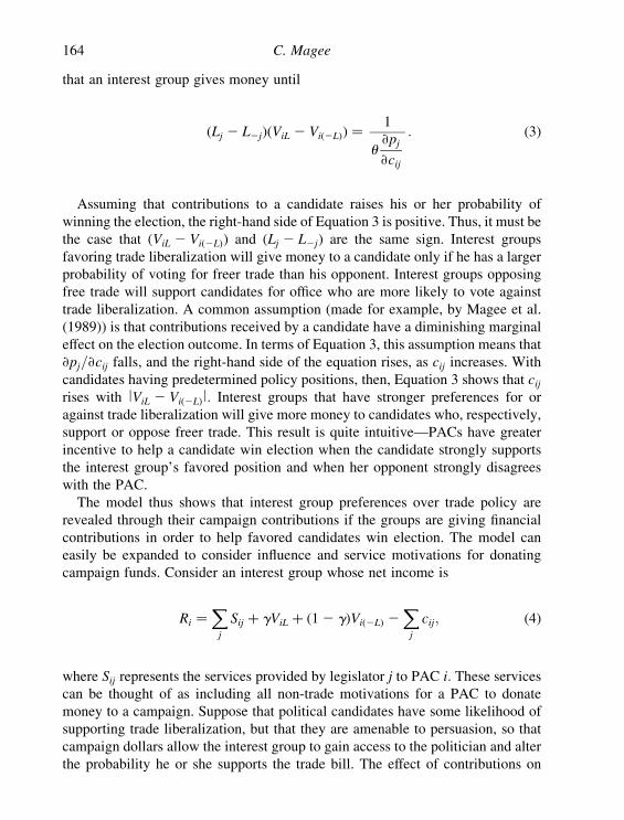
that an interest group gives money until

ðLj 2 L2jÞðViL 2 Við2LÞÞ ¼1

u›pj

›cij

: ð3Þ

Assuming that contributions to a candidate raises his or her probability of

winning the election, the right-hand side of Equation 3 is positive. Thus, it must be

the case that ðViL 2 Við2LÞÞ and ðLj 2 L2jÞ are the same sign. Interest groups

favoring trade liberalization will give money to a candidate only if he has a larger

probability of voting for freer trade than his opponent. Interest groups opposing

free trade will support candidates for office who are more likely to vote against

trade liberalization. A common assumption (made for example, by Magee et al.

(1989)) is that contributions received by a candidate have a diminishing marginal

effect on the election outcome. In terms of Equation 3, this assumption means that

›pj=›cij falls, and the right-hand side of the equation rises, as cij increases. With

candidates having predetermined policy positions, then, Equation 3 shows that cijrises with lViL 2 Við2LÞl: Interest groups that have stronger preferences for or

against trade liberalization will give more money to candidates who, respectively,

support or oppose freer trade. This result is quite intuitive—PACs have greater

incentive to help a candidate win election when the candidate strongly supports

the interest group’s favored position and when her opponent strongly disagrees

with the PAC.

The model thus shows that interest group preferences over trade policy are

revealed through their campaign contributions if the groups are giving financial

contributions in order to help favored candidates win election. The model can

easily be expanded to consider influence and service motivations for donating

campaign funds. Consider an interest group whose net income is

Ri ¼X

j

Sij þ gViL þ ð12 gÞVið2LÞ 2

X

j

cij; ð4Þ

where Sij represents the services provided by legislator j to PAC i: These servicescan be thought of as including all non-trade motivations for a PAC to donate

money to a campaign. Suppose that political candidates have some likelihood of

supporting trade liberalization, but that they are amenable to persuasion, so that

campaign dollars allow the interest group to gain access to the politician and alter

the probability he or she supports the trade bill. The effect of contributions on

C. Magee164

the probability the liberalization measure passes the legislature is

›g

›cij¼ u

›pj

›cijðLj 2 L2jÞ þ pj

›Lj

›cij

" #

: ð5Þ

Differentiating Equation 4 and substituting Equation 5 into the result shows that

PAC i gives money to candidate j until

›pj

›cijðLj 2 L2jÞ þ pj

›Lj

›cij¼

12›Sij

›cij

uVi

; when cij . 0; ð6Þ

where Vi ¼ ViL 2 Við2LÞ is the interest group’s net gain from liberalization. If the

interest group values the electoral and influence gains from contributing, it must

be the case that the marginal gain to the interest group in terms of services

provided by the candidate is less than one. The numerator in the right-hand side of

Equation 6 is thus non-negative, and it is strictly positive for PACs that hope to

affect election outcomes or to influence policy choices through their contributions.

The right-hand side of the equation, then, is positive for interest groups favoring

liberalization ðVi . 0Þ and negative for those opposing it.

The first term in Equation 6 represents the benefit to the lobby of helping a free

trade or protectionist candidate win election. The second term shows the gain from

changing the probability that candidate j supports the liberalization bill proposed.

These two terms correspond to the electoral and influence motives discussed

earlier for campaign contributions. In most models of probabilities, such as the

probit model, the effect of campaign contributions on the likelihood of a candidate

supporting a bill ð›Lj=›cijÞ is maximized when the candidate has a 50%

probability of supporting the trade deal. Thus, the influence motive pushes interest

groups to give money to candidates who are undecided. The electoral motive, on

the other hand, induces PACs favoring liberalization to give money to candidates

who are already strong supporters of free trade (meaning that there is a large

Lj 2 L2j in Equation 6). As long as the electoral motive is a consideration in its

contribution decisions, PACs favoring liberalization will concentrate their money

on candidates who are inclined to support free trade on average while lobby

groups favoring trade barriers will give money to candidates who are more

protectionist. Magee (2002) finds empirical evidence that PACs are motivated by

the desire to affect elections. On four out of five issues examined, including trade

policy, PAC contributions flowed more readily to 1996 candidates for the House

of Representatives who had already committed to supporting the interest group’s


preferred policy stance. Thus PACs will, in general, contribute more to candidates

who are likely to vote in the group’s interest.

The model shows that, with an electoral motive for giving contributions,

two different PACs both of which favor trade liberalization have incentives to

give contributions to the same group of candidates for office—those strongly

favoring free trade and whose opponents are protectionists. PACs favoring

protectionism have an incentive to give to a different group of candidates,

with all such protectionist interest groups concentrating their donations on

those candidates favoring trade barriers.

If interest groups give money primarily for reasons of gaining influence

with legislators, the prediction about patterns of PAC contributions is slightly

different. In this case, both PACs favoring trade liberalization and those

favoring protectionism will tend to give to the same group of candidates—

those with a high probability of winning election but who are undecided on

the trade liberalization issue. Thus, all interest groups who are concerned with

trade bills, whether protectionist or not, will give money to a similar group of

candidates. PACs whose interests lie in other areas of legislation, on the other

hand, will not necessarily concentrate their contributions on this same group

of candidates.

Finally, consider the case in which interest groups give money primarily to gain

unobservable services that legislators can provide. The ability for a legislator to

provide services to interest groups depends on holding positions of power in

Congress or membership on committees that deal with the policies the interest

group is concerned with. Thus, all PACs have an incentive to give contributions to

representatives who have achieved positions of power. PACs with common

concerns will tend to concentrate their donations on politicians who are members

of relevant committees. As with the influence motive, side of a policy debate

which the interest group favors is irrelevant in considering the relationship

between its contribution pattern across candidates and that of other interest groups.

Whether interest groups are motivated by electoral, influence, or service

considerations in giving campaign contributions, we should observe some positive

correlation between the contribution patterns for different PACs across candidates

since all PACs will concentrate their donations on those politicians most able to

provide services to interest groups. A larger correlation between two PACs’

contribution patterns will be evident when the groups are interested in the same

policy issues. The strongest correlation between two PACs’ contribution patterns

will occur when both interest groups are concerned with the same issues and have

the same preferences over the policies adopted. Examining how similar one

interest group’s contributions are to another group’s donations reveals the extent

to which the two groups have common interests in promoting certain policies.

C. Magee166

The following sections of the chapter examine the relationships between

different interest groups’ contribution patterns across candidates. The question

addressed is whether interest groups representing a common factor of production

have more similar contribution patterns than interest groups representing a

common industry. If corporate PACs are primarily interested in certain issues

while labor PACs are interested in other issues, for example, there will be a

stronger correlation between the contribution patterns of two corporate PACs (or

two labor PACs) than there will be between the contribution patterns of a

corporate and a labor PAC. If PACs are divided along industry lines, however,

there should be a significant positive correlation between the contribution

decisions of interest groups within the same industry.

Examining the relationships between contribution decisions of different

interest groups, then, reveals whether groups lobby along factor or industry

lines. This question is relevant for the debate over how mobile factors are across

industries and whether short or long-run goals are more important to PACs in

their lobbying efforts.

7.3. EMPIRICAL ANALYSIS

The data on PAC contributions were provided by the Federal Election

Commission. The data set includes only qualified and non-qualified non-party

PACs who gave money to at least one candidate for Congress in 1991–1992.

Independent expenditures against a candidate and communications costs against a

candidate are counted as negative contributions. There are 482 manufacturing

PACs whose industry and factor are identified, and they gave to 1988 candidates

for the House of Representatives and the Senate. Of these interest groups, 435 are

corporate interest groups and 47 are labor groups. The disparity in numbers

between corporate and labor groups reflects in part the difficulty of organizing for

labor unions relative to firms. Since many industries are dominated by a few large

firms, it is easier for them to overcome the collective action problems that plague

lobby groups. Unions, on the other hand, must successfully persuade many

different workers to sacrifice personally in pursuit of a collective good. As Olson

(1965) points out, the difficulties inherent in organizing a large group mean that

businesses will be better organized than labor. The small number of labor unions is

also a result of having a few large manufacturing labor groups rather than many

small ones.

Table 7.1 presents the correlations between the contribution patterns of PACs

for every pair of PACs in the data set. With 482 PACs, there are 115,921 pairs of

PACs that can be examined. Of these pairs of interest groups, 18,295 pairs


represent two PACs that do not share either a common factor of production (one is

corporate and one labor) or a common industry being represented. The correlation

between the contribution patterns across political candidates for such pairs of

groups is 0.0402. This correlation is significantly larger than zero at the 1%

significance level, with a t-statistic over 62. Thus, even among interest groups

with no clear connection, there is a tendency to give money to the same set of

candidates for the Senate and House of Representatives.

There are several important implications of this result. First, it suggests that

PACs are rational. Snyder (1992) and Stratmann (1992) have provided some

evidence that PAC contributions are motivated by rational considerations of self-

interest, and the results here support their conclusions. If an interest group gave

money to candidates purely because of a utility gain from participating in the

political system, there would be no correlation between the contribution patterns

of different interest groups (particularly between groups that do not represent

either the same factor of production or the same industry). The null hypothesis of

no correlation is emphatically rejected by the data, however, as the model in

Section 7.2 suggests it should be when PACs are motivated by self-interested

factors.

A second implication of the positive correlation between the contribution

patterns of unrelated interest groups is that the electoral motive for giving money

does not dominate the service and influence motives. Suppose for the moment,

that interest groups cared only about which candidates were elected to Congress

and they never sought influence or used contributions as a means of gaining

Table 7.1: Correlations between PAC contribution patterns, by type of PAC.

Standard errors are in parentheses. Numbers of observations in each cell are in brackets.

**Means are significantly different at the 1% level.

C. Magee168

services from politicians. Suppose furthermore that interest groups and candidates

for office were split along factor lines so that each candidate and each PAC could

be considered labor friendly or business oriented. With an electoral motive for

giving contributions, special interest groups with an interest in helping labor-

friendly candidates win election would concentrate their money on labor-friendly

candidates who are engaged in a tight election. Interest groups representing

capital, meanwhile, would focus their contributions on a separate group of

candidates. Thus, we would observe a negative correlation between the

contribution pattern of a labor and a capital interest group, on average.

With an influence motive for giving campaign contributions, on the other hand,

both capital and labor groups would give money to the same set of moderate

candidates who are likely to win election and whose policy positions can be

swayed the most by lobbies with access to the candidate. The service motive gives

all interest groups an incentive to give money to the same group of politically

powerful legislators who are in positions that make them capable of providing

direct aid to lobby groups in the form of setting the legislative agenda, marking up

bills in committees, and pressurizing fellow congress members to vote in a certain

way. The influence and service motivations for campaign contributions, contrary

to the electoral motive, then, predict that unrelated interest groups will tend to give

money to the same set of candidates for office. This prediction is found to have

empirical support.

Table 7.1 reveals that when two PACs represent a common industry, there is a

significant increase in the correlation between their contribution patterns (the

correlation increases to 0.0618). Similarly, if the two interest groups represent a

common factor of production (both are capital or labor), the correlation between

their contribution patterns increases to 0.0667. Finally, if the two PACs share a

common factor and represent the same industry, there is a still greater correlation

between their contribution patterns across candidates (0.1058). These higher

correlations between contribution patterns of PACs when they share more

common characteristics are consistent with the predictions of the theoretical

model in Section 7.2. The model there shows that the more two interest groups

have in common, the greater their incentive to contribute to the same set of

representatives.

Table 7.2 presents the correlations between contribution patterns within PACs

representing capital and those representing labor. There were 20,445 pairs of

interest groups in which one PAC represented capital and the other represented

labor. The average correlation between the contribution patterns of these pairs of

PACs was 0.0424. This mean is significantly greater than zero (the t-statistic is

over 67). When both interest groups were labor unions, the average correlation

between their contribution patterns was 0.0646. This mean was significantly


higher ðt ¼ 7:6Þ than the average correlation between contributions from a labor

group and a corporate group. The correlation between two corporate groups’

contribution patterns was 0.0714, which was also significantly higher ðt ¼ 35:4Þthan the average correlation between contributions from a labor group and a

corporate group. Interestingly, two separate corporate lobbies have more similar

contribution patterns on average than two labor unions—the t-statistic examining

the difference in the mean correlations between two corporate lobbies and two

labor lobbies is t ¼ 2:0; indicating that the means are different at the 5%

significance level. It is difficult to judge whether this difference is economically

significant as well. One explanation for this difference is that labor groups seem to

be more likely to give money to challengers than corporate PACs do. Whereas

businesses focus their lobbying efforts on Congress members who have been in

office for a number of terms and have accumulated power in the government, labor

groups do not place such weight on a candidate being a well-entrenched member

of Congress. Magee (2002), for instance, shows that being a committee chair and

an incumbent significantly increased the contributions a candidate received from

business groups in 1996 races for the House of Representatives, but the two

variables had no effect on money received from labor groups.

Table 7.3 examines whether or not corporate and labor PACs have similar

correlation patterns for those groups within the same industry and for those from

separate industries. The first column in Table 7.3 includes only every pair of two

capital PACs, and these pairs of PACs are broken into those that represent

a common industry and those that represent separate industries. The second

column includes only pairs in which both PACs represent the interests of labor.

Table 7.2: Correlations between PAC contribution patterns, by factor types.

Standard errors are in parentheses. Numbers of observations in each cell are in brackets.

*Means are significantly different at the 5% level. **Means are significantly different at

the 1% level.

C. Magee170

The estimates show that corporate PACs that are in the same industry have a

significantly higher correlation between their contribution patterns than corporate

groups representing different industries. For labor groups, however, the average

correlation in contribution patterns between PACs within the same industry is not

significantly different from the average correlation in contributions between PACs

representing separate industries.

Why might there be a greater correlation between PACs within the same

industry for capital groups but not for labor groups? One possible explanation

might be that capital is less mobile across industries than labor, as is commonly

assumed in specific factors models. If labor is perfectly mobile, then industry is

irrelevant in unions’ lobbying efforts. In the Heckscher–Ohlin model with perfect

factor mobility, for instance, industry affiliation is irrelevant for interest groups’

position on trade policy. All groups representing a factor of production either

benefit from free trade and support it politically or are harmed by free trade and

oppose it. Thus, with perfect factor mobility, the relationship between the

lobbying patterns of two interest groups is independent of industry. This

prediction is consistent with the result that the correlation of contribution patterns

between two labor unions within the same industry is no different than the

correlation between two unions from separate industries.

If factors are immobile across industry lines, however, their fortunes rise or fall

with those of their industry. Thus, pressure groups within a particular industry

have a common interest in promoting policies that benefit the industry. The

assumption of immobile factors, then, generates the prediction that groups

representing the same industry will tend to contribute to the same set of policy

makers more often than interest groups representing different industries. This

prediction fits well with the observation that for capital groups there is a much

Table 7.3: Correlations between PAC contribution patterns, by industry type.

Standard errors are in parentheses. Numbers of observations in each cell are in

brackets. **Means are significantly different at the 1% level.


higher correlation ðt ¼ 32:3Þ between corporate PACs within the same industry

than between corporate PACs from separate industries.

The implication that capital is less mobile across industries than labor is very

tentative. Examining the correlations between interest group contribution patterns

is not a direct test of mobility, and there are other possible explanations for the

result that corporate groups within industries have more similar contribution

patterns than corporate PACs from separate industries. One possible explanation

is that corporate groups and labor groups have different motivations in giving

campaign contributions. Suppose that firms care primarily about securing services

from politicians on committees relevant to their industry. In this case, defense

industry firms will concentrate their donations on powerful members of national

security committees in the House and Senate while the oil and gas industry

focuses on members of the energy and commerce committee. Thus, there is a

strong correlation between corporate contributions from groups within the same

industry. If labor groups give money primarily with a motivation of helping

certain candidates win election, on the other hand, it is not clear that there should

be a larger correlation in the contribution patterns of labor PACs within the same

industry than there is in the contributions of labor PACs from different industries.

Table 7.4 presents the estimates from a regression in which the dependent

variable is the correlation between two interest groups’ contribution patterns. In

the first column, the determinants of the correlation are assumed to be the factors

examined in Table 7.1: irrespective of whether the two interest groups represented

the same factor and the same industry. In column 2, the factor variable is separated

into two different variables. One is a dummy variable indicating whether or not

both interest groups represent corporate interests (capital ¼ 1, if they do), and the

second is whether or not both interest groups represent labor unions (labor ¼ 1, if

they do). The final column breaks the same industry variable down into separate

dummy variables for each industry.

The results in Table 7.4 are similar to those in Tables 7.1–7.3. Representing the

same factor of production and a common industry, both increase the correlation

between two interest groups’ contribution patterns. The larger coefficient estimate

suggests that representing a common industry is slightly more important than

representing the same factors of production in determining how similar the

contribution patterns of two PACs are. The difference between the two coefficient

estimates in column 1 is statistically significant at the 1% level. Consistent with

the result in Table 7.2, the second column of Table 7.4 shows that two corporate

PACs have more similar contribution patterns than two labor groups do (after

controlling for whether or not the two PACs are in the same industry). When both

interest groups are corporate, the correlation between their contribution patterns

C. Magee172

rises by 0.0285, compared to a 0.022 increase when both groups represent the

interests of labor. These coefficients are significantly different at the 5% level.

In column 3, 15 of the 20 coefficient estimates on the industry dummy variables

are positive, with 11 of these coefficients being statistically significant at the 1 or

5% level. There was a significant negative effect of having two PACs within the

same industry on the correlation between their contribution patterns for only

one industry, food and kindred products. This result is likely to be a Type I error.

The coefficient estimate is very small in magnitude, but because of the large

number of PACs representing this industry, it is statistically significantly different

from zero. Several of the coefficient estimates are quite large. When both PACs

Table 7.4: Determinants of PAC contribution correlations.

Variables Coefficients Coefficients Coefficients

Same factor 0.0284**

Both capital 0.0285** 0.0285**

Both labor 0.0220** 0.0224**

Same industry 0.0363** 0.0363**

Oil and gas 0.0455**

Food 20.0086**

Tobacco 0.3285**

Textiles 0.0501**

Apparel 20.0038

Lumber 0.0643**

Furniture 20.0191

Paper 0.1477**

Printing 0.0295

Chemicals 0.0389**

Rubber 20.0042

Leather 0.2605*

Stone, clay, glass 0.0671**

Primary metals 0.0119*

Fabricated metals 0.0031

Machinery 0.0039

Electronic equipment 0.0415**

Transportation 0.0990**

Instruments 20.0062

Miscellaneous 0.0013

Constant 0.0386** 0.0386** 0.0384**

F-statistic for capital, labor 607.27 615.59

F-statistic for industry variables 157.82

R2 0.0369

Observations 115,921 115,921 115,921

* Coefficients are significant at the 5% level. **Coefficients are significant at the 1% level.


are in the tobacco industry, the correlation between their contribution patterns rose

by 0.33. This large estimate may indicate a high degree of coordination between

lobby groups within the tobacco industry, or it may have occurred by random

chance since there were only 11 PACs representing the interests of tobacco in the

data set. There are similarly small numbers of PACs representing the other

industries with very large coefficient estimates, such as the paper (seven PACs)

and leather (two PACs) industries. The industries with the largest numbers of

PACs were the food and kindred products industry, with 128 interest groups

representing it, and the chemicals and allied products, with 105 PACs.

7.4. CONCLUSION

This chapter has presented a theoretical model showing that all interest groups

have incentives to concentrate their campaign contributions on a similar set of

candidates for office. PACs with common policy preferences have even greater

incentives to give money to common groups of candidates. The empirical

evidence supports these predictions. Even among interest groups that did not share

a common factor of production and did not represent the same industry, the

correlation between their contribution patterns in 1991–1992 was 0.04, which was

significantly greater than zero. When PACs represented the same factor of

production, the same industry, or both, the correlation between their contribution

patterns was significantly higher. Interestingly, the contribution patterns of two

corporate lobby groups were more similar, on average, than the contribution

patterns of labor unions.

When factors are partially mobile across sectors, the short-run interests of lobby

groups will depend on the industry they represent while the long-run interests

depend on the factor of production. If trade liberalization harms the textile

industry but raises the overall return to capital in the economy, for example, then

capital owners in the textile industry may suffer short-run losses as the textile

industry declines, but in the long run, after the capital has moved to more

prosperous industries the capital owners will gain from the liberalization.

Lobbying for short-run gains, then, suggests that groups from the same industry

will have the most in common in their contribution patterns. If groups lobby

primarily for long-run gains, then groups representing the same factor of

production will have similar contribution patterns. The results in this chapter

indicate that both short and long-run considerations play a role in determining

interest group contribution decisions, because both representing a common

industry and representing the same factor of production increase the similarity

between two lobbies’ contribution patterns.

C. Magee174

REFERENCES

Beaulieu, E. and Magee, C. (2004). Campaign contributions and trade policy: new tests of

Stolper–Samuelson. Economics and Politics, in preparation.


833–850.

Grossman, G. and Helpman, E. (1996). Electoral competition and special interest politics.

Review of Economic Studies, 63, 265–286.

Hall, R. and Wayman, F. (1990). Buying time: moneyed interests and the mobilization of

bias in congressional committees. American Political Science Review, 84(3), 797–820.

Hartigan, J. and Tower, E. (1982). Trade policy and the american income distribution.

Review of Economics and Statistics, 64, 261–270.

Magee, S. (1980). “Three simple tests of the Stolper–Samuelson theorem,” in Issues in

International Economics, P. Oppenheimer, (ed.), London: Oriel Press, pp. 138–153.

Magee, C. (2002). Do political action committees give money to candidates for electoral or

influence motives? Public Choice, 112, 373–399.

Magee, S., Brock, W. and Young, L. (1989). Black Hole Tariffs and Endogenous Policy

Theory, Cambridge: Cambridge University Press.


Snyder, J. (1992). Long-term investing in politicians; or, give early, give often. Journal of

Law and Economics, 35, 15–43.

Stratmann, T. (1992). Are contributors rational? Untangling strategies of political action

committees. Journal of Political Economy, 100, 647–664.


CHAPTER 8

Sweetening the Pot: How American

Sugar Buys Protection

OMER GOKCEKUSa,*, JUSTIN KNOWLESb, andEDWARD TOWERc

aJohn C. Whitehead School of Diplomacy and International Relations, Seton Hall University,

400 South Orange Avenue, South Orange, NJ 07079, USAbWharton School, University of Pennsylvania, Jon M. Huntsman Hall, 3730 Walnut Street,

Philadelphia, PA 19104-6340, USAcDepartment of Economics, Duke University, Box 90097, Durham, NC 27708-0097, USA

Abstract

We use Probit and Tobit analysis to explore the determinants of campaign

contributions from the sugar industry to Senators from 1989 to 2002. We find that

the power and willingness of Senators to protect sugar influence campaign

contributions significantly: serving on the Senate Agriculture Committee attracts

$4266 of contributions per election cycle; serving on the relevant subcommittee

that deals with sugar legislation is worth an additional $2179 for a total of $6445;

membership of the majority party $1235; and an impressionable freshman Senator

from a sugar cane state receives $7367 more than a more senior senator from a

non-sugar state.

Keywords: Sugar industry, lobbying, trade protectionism

JEL classification: F13



It could probably be shown by facts and figures that there is no

distinctively American criminal class except Congress (Mark Twain,

Pudd’nhead Wilson’s New Calendar).

8.1. INTRODUCTION

Kraft Foods is moving Life Savers production and its 600 jobs, to

Canada. One reason: Sugar is cheaper there. Unlike the US government,

Canada doesn’t prop up prices to protect a handful of domestic sugar

growers (USA Today, 2002).

When economics collides with politics in the halls of Congress, politics

usually wins (Smith, 2002).

The US sugar program is a case in point to show that indeed trade policies

redistribute domestic wealth. In particular it shows what happens when the

beneficiary of a protectionist policy is a small and concentrated group and the

losers are large and widely disbursed all over the country. Sugar growers have

been capturing rents from tariffs and quotas since the 1790s. Taussig (1931)

described sugar protection in his Tariff History of the United States. The US

General Accounting Office (2002) estimated that the sugar program cost

consumers about $1.5 billion in 1996 and about $1.9 billion in 1998. As

Groombridge (2001, p. 1) has written: “nowhere is there a larger gap between the

US government’s free trade rhetoric and its protectionist practices than in the

sugar program.”

A number of researchers have examined the US sugar program. See, for

instance, Harper and Aldrich (1991), who examine the determinants of

congressional voting on the US sugar program, Borrell and Pearce (1999) who

examine the effects of worldwide sugar protection, Lopez (2001), and the articles

in Marks and Maskus (1993).

In this paper, after briefly describing the US sugar program and reporting on

its welfare consequences, we focus on an overlooked aspect of it: the institution

of rent seeking, in particular how the sugar industry—an interest group—picks

legislators to support with campaign contributions. We examine sugar industry

contributions to the reelection campaigns of US Senators for the 14 years from

1989 to 2002. During this period of time, as part of three consecutive Farm

Bills, those in 1991, 1996 and 2001, both Houses voted against phasing out

price supports for sugar, and they extended the federal sugar program. We

attempt to shed light on the relationship between sugar industry contributions

and incumbent Senators’ attributes. In particular, we analyze the premium

O. Gokcekus, J. Knowles, and E. Tower178

attached to the power and willingness of Senators to maintain protectionist

sugar policies, and consequently to supply the rent collected by sugar producers.

Our analysis shows that there is a systematic targeting by the sugar industry in

the allocation of contributions among incumbent Senators. Membership of the

majority party, serving on the Senate Agriculture, Nutrition and Forestry

Committee, and serving on the Senate Agricultural Production, Marketing, and

Stabilization of Prices Subcommittee (which oversees the sugar program) all

attract money.

8.2. THE US SUGAR PROGRAM

The Coalition for Sugar Reform (2003) provides a succinct description of the US

sugar program:

The Federal Government has operated the current price support program

since 1981 to subsidize sugar beet and sugarcane producers and

processors by maintaining high sugar prices. The government supports

the price by restricting the supply of sugar made available to consumers.

It does so by limiting imports. There are no restrictions on domestic sugar

production or marketing. [There are two main components of the

program: Price support loans and import restrictions.]

8.2.1. Price support loans

Under the program, the Government makes loans available to sugar beet and

sugarcane processors. Sugar loans are unique in that they are made to

processors (corporations or cooperatives) rather than to individual farmers, as

under other farm programs. In order to be eligible for a loan, the processor must

pay the producer a Government-specified minimum price for sugar beets or

sugarcane. Processors pledge the sugar as collateral to obtain a so-called “non-

recourse” loan from the Government… When the loan matures, the processor

must decide whether he will make more money by (1) paying off the loan, plus

interest, and redeeming the pledged sugar; or (2) forfeiting the sugar and

keeping the Government’s money… (T)o avoid loan forfeitures… (the US

Department of Agriculture) restricts imports to maintain the…price of sugar

high enough so that processors will have an incentive to redeem every pound of

sugar placed on loan.

Sweetening the Pot: How American Sugar Buys Protection 179

8.2.2. Import restrictions

As mentioned earlier, the Government supports the price of sugar by restricting

imports. It is able to do so because sugar is a deficit crop—we consume more than

we produce. Every quota year (October/September) USDA establishes an overall

Tariff Rate Quota (TRQ) for sugar, which is prorated among some forty nations by

the US Trade Representative on the basis of import history during the period

1975/81. If during the course of the year more sugar is needed, the quota can be

increased. If a nation cannot fill its quota, a deficit can be declared and reassigned

to other quota holding nations… Sugar can enter in excess of the TRQ, but the

importer would have to pay a duty of around 16 cents a pound, which normally

would make it unprofitable.

8.3. CONSEQUENCES OF THE PROGRAM

The Agriculture Committee is writing a new farm bill, and we cannot

afford to have the sugar lobby write the sugar policy. Until the Sugar

Subsidy Program is phased out, costumers will pay more for products

containing sugar. Taxpayers will continue to pay more to buy surplus

sugar.Workers in the candy and the cane refining industry will continue to

lose their jobs. The sugar program will continue to benefit a few, without

solving the problems of family farmers. We must insist on real reform in

the sugar program, and end the regulations that are costing Americans

money and American jobs (Congressman W.O. Lipinski, 2001).

The gap is wide between US and world sugar prices. As Figure 8.1 (drawn from

Table 1 of Appendix I of USGAO, 2002) shows, in 1998 the US raw sugar price

was more than double the world price. Between 1985 and 1998, on average the US

raw sugar price was 3.2 times the world raw sugar price.

Welfare Implications. The US General Accounting Office (2002) recently

examined the US sugar program. We quote their statement of their major findings.

8.3.1. Increases users’ costs

We estimate that the sugar program cost domestic sweetener users about $1.5

billion in 1996 and about $1.9 billion in 1998. Sweetener users included (1)

sugarcane refiners that bought raw cane sugar, (2) food manufacturers that bought

refined sugar and other sweeteners, and (3) final consumers who bought

sweeteners and sweetener-containing products…


8.3.2. Benefits for producers

The primary beneficiaries of the sugar program’s higher prices are domestic sugar

beet and sugarcane producers who, we estimate, received benefits of about $800

million in 1996 and about $1 billion in 1998. About 70 percent of the benefits went

to sugar beet growers and processors. Sugarcane producers received about 30

percent of the benefits.

High Fructose Corn Sweetener (HFCS) producers received little, if any, benefit

from the sugar program in either 1996 or 1998, according to our current model’s

estimates. This result contrasts with our finding in 1993. At that time, HFCS cost a

few cents per pound less than domestic sugar, and both products cost about twice

as much as sugar on the world market… [T]he possibilities for substitution

between sugar and HFCS are more limited than in prior years because

technological advances have improved HFCS products and created more

specialized sweetener markets. As a result, even if the sugar program were

removed and the price of domestic sugar fell substantially, the impact on the price

of HFCS would be limited… Executives from the Corn Refiners’ Association,

which represents HFCS manufacturers, agreed with our model’s results as they

pertained to HFCS, stating that HFCS producers do not benefit from the sugar

program because domestic HFCS prices are no longer linked to sugar prices.

Figure 8.1: The world and US sugar prices (source: GAO/RCED-00-126, p. 14).


8.3.3. Net effect

We estimate that the sugar program resulted in net losses to the US economy of

about $700 million in 1996 and about $900 million in 1998. Our net loss estimates

include economic inefficiencies and transfers to foreign producers. Economic

inefficiencies occurred, for example, when the sugar program’s artificially high

domestic prices encouraged farmers to grow sugar beets instead of another crop,

such as wheat, that, without the sugar program, might have been relatively more

profitable. Inefficiencies also occurred when artificially high sugar prices

discouraged consumers from purchasing sugar. The cost of these inefficiencies

totaled about $300 million in 1996 and about $500 million in 1998. Transfers from

the US economy to foreign producers occurred because foreign producers received

artificially high prices for the raw sugar they exported to the United States. We

estimate that these transfers amounted to about $400million in both 1996 and 1998.

8.4. SUGAR INTEREST GROUPS’ CONTRIBUTIONS

The industry makes so much money through federal price supports that it

can afford to spend a lot to win political influence in Washington… Just

plain and simple, it’s money to a small group of growers. When you are

getting that kind of money, you can work hard to preserve it. What they

are doing is protecting money, protecting wealth, and protecting higher

incomes (A Capitol Hill Sugar Expert, 1998).

Despite its relatively small size, the US sugar growing industry (henceforth sugar)

is one of Congress’ main campaign contributors. On average, from 1989 to 2002,

sugar contributed $3,090,710 in each election cycle, i.e., $1,545,355 annually, to

incumbents in their campaigns.1Table 8.1 summarizes the total sugar contributions

1 The source of the data is the web page of the Center for Responsive Politics, www.opensecrets.com,

which utilizes reports filed to the Federal Election Committee. They are based on contributions of $200

or more from Sugar grower PACs and individuals to federal candidates and from individual and soft

money donors to political parties, as reported to the Federal Election Commission. Consistently, more

than 90% of the contributions were made by a small number of organizations. For instance in the 107th

Congress, these organizations are Flo-Sun Inc., American Crystal Sugar, American Sugar Cane

League, US Sugar Corp., Southern Minn Beet Sugar Co-op., American Sugarbeet Growers Assn,

Florida Sugar Cane League, Minn-Dak Farmers Co-op., Great Lakes Sugar Beet Growers, Florida

Sugar Cane League, Snake River Sugar, Sugar Cane Growers Co-op. of Florida, US Beet Sugar Assn,

Rio Grande Valley Sugar Growers, and Amalgamated Sugar. The contributions are in real terms, i.e., in

107th congress dollars. We use the consumer price index (CPI relative to the average CPI in 2001 and

2002) as the deflator.


for the last seven congresses, i.e., The 101st–107th Congresses. In addition to the

total contributions, this table gives the type of contributions, i.e., individual, PACs,

and Soft Money. It also shows how the total contributions were allocated between

two parties. An examination of the aggregate sugar campaign contributions since

1989 reveals interesting patterns.

First, clearly, soft money has become more important. This is an interesting

pattern because “soft money” contributions are not subject to the limits and

regulations of federal election laws. Soft money contributions are described as the

main vehicle for wealthy individuals, corporations, and labor unions to deliver

millions of dollars to political parties without regard for the limits and other

requirements of the law (Center for Responsive Politics, 1998). Sugar has utilized

this vehicle intensively. Second, incumbent representatives from the Democratic

Party have received 57% of the contributions to incumbents.

However, as is presented in Figure 8.2, whether the party is majority or not also

played a role. Our regression analysis shows that, when not in the majority, the

Democratic Party attracted 50% of contributions and the Republican Party

attracted 38%, with 12% more attracted by the majority party, which is either the

Democratic or Republican party. This means that sugar does take into account the

potential influence ( power) of a party in allocating its contributions.

There is a substantial literature in the political science and public choice areas

on campaign contributions and how interest groups allocate the contributions

among legislators, (e.g., Munger, 1989; Grier et al., 1990). In Section 8.5, we

adopt a model, which is built on the premise that the size of contributions for

reelection depends on a legislator’s characteristics. In particular, we explore the

relationship between campaign contributions and the incumbent Senators’ party

affiliation, state, seniority, relevant committee and subcommittee memberships.

Table 8.1: Campaign contributions by sugar interest: 1989–2002.

Congress Total (in $) Individual (%) PACs (%) SOFT (%) To Democrats (%)

101st 2,571,056 9 91 NA 60

102nd 2,729,790 17 71 11 67

103rd 2,841,146 9 79 12 65

104th 3,916,350 12 61 26 46

105th 3,059,715 9 65 25 52

106th 3,561,589 9 47 44 52

107th 2,955,323 8 67 25 56

Totals are in real terms, i.e., in 107th congress dollars. The deflator is the CPI. All tables, figures, and

discussion refer to a typical two-year election cycle.


8.5. DETERMINANTS OF SUGAR’S CAMPAIGN CONTRIBUTIONS

In this section we check the association between campaign contributions and

different characteristics of an incumbent Senator. We are effectively testing the

validity of four prior assertions, which were developed by reviewing the literature

on campaign contributions by interest groups to incumbent Senators.

First, we examine the relationship between campaign contributions and party

affiliation. To capture both Senators’ power and willingness to provide what sugar

interests want, we conduct two sets of analyses. We examine the contributions to

Democratic and Republican Senators. As Table 8.2 shows, incumbent Senators

affiliated with the Democratic Party received 43% more than incumbent

Republican Senators. We initially took this as an indicator of the premium

attached to the “ideology or reputation for particular policy belief”, e.g.,

Democrats are protectionist and Republicans support market solutions. But this

finding contrasts with the results from our more sophisticated analysis presented

below. That analysis uses probit and Tobit regressions to show that correcting for

other factors, party does not matter. It demonstrates the importance of model

building to understand how campaign contributions are allocated.

Figure 8.2: Allocation of sugar campaign contributions between two political parties. Results from

regressing each party’s Share of Contributions over the seven Congresses (14 observations) on

Majority Party, which is one for the ruling party in the Senate and zero otherwise, and Democrat, a

dummy which is 1 or 0 depending on whether the party is Democratic. The intercept is 38%, and both

coefficients of the Democratic and Majority Party dummies are 12%.


We also examine the contributions to incumbent Senators according to their

membership of the Majority party: Incumbent Senators who were members of the

majority party received 40% more than incumbent Senators in the minority party.

We interpret this as an indicator of the premium collected for the “institutional

power or productivity,” of the Senator due to his party affiliation.

Second, we explore the relationship between campaign contributions and the

state a Senator represents. We hypothesize that the Senators who have a large

presence of sugar producers in their states receive larger campaign contributions

than the other Senators, because it is easier to get them to vote on behalf of sugar,

i.e., they are more willing. In particular, we check to see if there is a difference

between Senators from the four sugar cane states—Florida, Hawaii, Louisiana,

Table 8.2: Determinants of campaign contributions by sugar interest to incumbent Senators.

Average(in 2002 dollars)

Percent ofSenators received

Average(among those who received)

Party

Democrat $6061 52% $11,661

Republican $4230 46% $9121

Ratio 1.43 1.12 1.28

Sugar states

Sugar Cane State $8923 71% $12,583

Not a Sugar state $3979 42% $9412

Ratio 2.24 1.68 1.34

Sugar Beet $7643 64% $11,933

Not a Sugar state $3979 42% $9412

Ratio 1.92 1.52 1.27

Majority Party

Majority Party $5940 52% $11,405

Minority Party $4230 46% $9219

Ratio 1.40 1.14 1.24

Committees

Agr. Committee $10,778 69% $15,568

Not Agr. Comm. $3889 45% $8693

Ratio 2.77 1.55 1.79

Sub-committee $11,722 75% $15,629

Not Agr. Comm. $3889 45% $8693

Ratio 3.01 1.68 1.80

Seniority

Freshman $6800 61% $11,068

Sophomore $5683 49% $11,650

Junior $4508 42% $10,805

Senior þ $2687 38% $7023

All members $5168 49% $10,487


and Texas, and Senators with no sugar industry among their constituency; and

whether there is a difference between Senators from the eleven Sugar Beet

States—California, Colorado, Idaho, Michigan, Minnesota, Montana, Nevada,

North Dakota, Oregon, Washington, and Wyoming, and Senators with no sugar

industry among their constituency. As Table 8.2 shows, Senators from sugar cane

states receive 124% more, and Senators from sugar beet states receive 92% more

than the Senators with no sugar industry within their constituency, with the

difference presumably reflecting the smaller size of the sugar beet sector.

Third, we assess the relationship between campaign contributions and seniority

in the Senate. Seniority could be seen as a proxy for electoral security and also

procedural expertise and collegial respect. There is empirical evidence that

freshmen Senators are perceived overall as being less secure and they usually

receive more than the others (Endersby and Munger, 1992; Grier et al., 1986;

Grier and Munger, 1993). Sugar gives almost 50% more money per capita and

more frequently to freshman Senators than the others.

Finally and fourth, we explore the relationship between committee and also

subcommittee memberships and campaign contributions. “Each committee has

significant power to veto, or at a minimum delay substantially, legislation within

its jurisdiction, to an extent determined by specific rules of the Senate, particularly

when committee control over the conference stage of bills is taken into account.

Committees, therefore, have both agenda and proposal control denied to

nonmembers. Further, even after a bill is passed and is being administered or

regulated by the bureaucracy, the committee with oversight jurisdiction has

substantial power to influence the administrative agency through hearings, agency

appointments, and appropriations.” (Grier and Munger, 1993, p. 619). In

particular, we focus on the Agriculture, Nutrition and Forestry Committee and

the Production and Price Competitiveness Subcommittees.

“The Senate Committee on Agriculture, Nutrition, and Forestry has helped

establish, guide, and examine agricultural policies here and abroad. It has had a

hand in fashioning the research and teaching of the 1860s, the price and income

support controls of the 1930s, and the international trade of the 1990s.” (US

Government Printing Office, 1998, p. 2) In particular, as part of the Farm

Bill, every five years, the committee revisits the sugar price–support program. As

a result of the division of labor within the committee the sugar price–support

program is in the responsibility area of the Production and Price Competitiveness

Subcommittee.2 As Table 8.2 presents, the committee members receive 177%

2 Until the early 1990s, the name of the same subcommittee was Agricultural Production, Marketing,

and Stabilization of Prices.


more; and subcommittee members receive 201% more than non-committee

members.

These preliminary cross-tabulations provide supporting evidence on all four of

our prior assertions. Clearly, sugar knows what it is doing: make the most out of

the money contributed by a systematic targeting according to Senators’ power and

willingness to provide what sugar wants.

To focus on and magnify this pattern, we further divide our sample into groups.

As Figure 8.3 shows, sugar targets the powerful: a non-committee member

minority party Senator receives only $3329 from sugar; a Senator from the

majority party who is also a member of the subcommittee receives 4.06 times as

much, i.e., $13,530 in an election cycle.

Figure 8.4 summarizes another salient future of targeting by the sugar industry,

namely targeting willing incumbent Senators: sugar contributes more to both

incumbent Senators from a sugar cane state and to freshmen Senators. For

instance, a freshmen Senator from a sugar cane state receives $24,009. On the

other hand, an incumbent Senator who is neither a freshman nor from a sugar state

receives only $3567.

The analysis in this section shows that indeed, Senators’ attributes matter—they

impact the contributions from the sugar industry to the reelection campaigns of the

incumbent Senators. However, it does not answer the following critical questions:

Figure 8.3: Sugar contributions and Power.


How much does each one of these attributes impact campaign contributions?

In other words, what is the marginal impact of different attributes on campaign

contributions?

Accordingly, Section 8.6 represents an attempt to move beyond this section’s

finding that attributes of Senators matter, and to open up consideration of partial

effects of different attributes. In other words, we examine the effect of attributes,

holding other attributes constant. First, we examine the partial impact of Senators’

attributes on the probability of receiving contributions from the sugar industry.

Second, we examine the partial impact of Senators’ attributes on the amount of

contributions received from the sugar industry.

8.6. MARGINAL EFFECTS OF DIFFERENT ATTRIBUTES ON THE

PROBABILITY OF GETTING MONEY AND THE AMOUNT OF

MONEY RECEIVED BY INCUMBENT SENATORS

First, we ask the simple question: How do different attributes affect the probability of

getting contributions fromsugar?Toanswer this questionwe estimate a probitmodel.

An incumbent Senator either receives contributions ðC ¼ 1Þ or does not ðC ¼

0Þ in an election cycle.3As is argued in Section 8.5, we believe that each Senator is

Figure 8.4: Sugar contributions and Willingness.

3 For details, see Greene, 2003, pp. 665–668.


unique and possesses a certain combination of attributes. We believe that a set of

attributes, such as PARTY, FRESHMAN, SUGAR CANE STATE, SUGAR

BEET STATE, COMMITTEE, and SUBCOMMITTEE, gathered in a vector x

explain the decision of the sugar industry whether to contribute, so that

ProbðC ¼ 1Þ ¼Fðx;bÞ;

ProbðC ¼ 0Þ ¼12 Fðx;bÞ;

where the set of parameters b reflects the impact of x on the probability.4

Briefly, REPUBLICAN is dummy variable, which takes on the value of 1 for a

Republican and the value of 0 for others. The variable, MAJORITY PARTY, is

also a dummy variable, which takes the value of 1 for a Senator who is a member

of the majority party during the election cycle and the value of 0 for others.5

FRESHMAN dummy takes on the value of 1 for a Senator who is in her first term.

SUGAR CANE STATE dummy takes the value of 1 for Senators who are from

four states with significant sugar cane production. These states are Florida,

Hawaii, Louisiana, and Texas. Similarly, SUGAR BEET STATE dummy variable

takes the value of 1 for Senators who are representing eleven states with a

significant sugar beet production. These states are California, Colorado, Idaho,

Michigan, Minnesota, Montana, Nevada, North Dakota, Oregon, Washington, and

Wyoming. Finally, the vector x includes two Committee membership dummy

variables: AGR. COMMITTEE dummy takes the value of 1 for Senators who are

members of the Senate Agriculture, Nutrition and Forestry Committee, and 0

otherwise; and PR. SUBCOMMITTEE dummy takes the value of 1 for Senators

who are members of the Senate Agriculture, Nutrition and Forestry Committee

and serve on the Agricultural Production, Marketing, and Stabilization of Prices

Subcommittee.

Table 8.3 presents the estimated coefficients and marginal effects for the probit

model.6 The model predicts that changing party affiliation from Republican to

Democratic increases the probability of getting contributions from sugar by 5%

points. Being a member of the majority party increases the probability of getting

contributions by 4% points. A freshman has a 17% point higher probability of

4 We use the normal distribution in our analysis, i.e., ProbðC ¼ 1Þ ¼Ðb0x21

fðtÞdt ¼ Fðb0xÞ ¼ Fðx;bÞ;

where F(·) is the notation for the standard normal distribution.5 Democrats were the majority for four of the congress, namely the 101st, 102nd, 103rd, and 107th; and

Republicans were the majority three times: the 104th, 105th, and 106th Congresses.6 To capture the potential impact of the number of years in Senate, we included an incumbency variable

in various functional forms, e.g., linear or second order polynomial. We could not get any significant

results. Therefore, for simplicity, we decided not to include years of incumbency in the model that we

present.


getting money for her reelection campaign from sugar. A Senator from a sugar

beet state has a 20% point, and a Senator from a sugar cane state has a 33% point

higher probability of getting contributions.

Finally, in their reelection campaigns members of the Senate Agriculture,

Nutrition and Forestry Committee have a 17% point higher probability of getting

money. If a member of this committee is also a member of the Agricultural

Production, Marketing, and Stabilization of Prices Subcommittee, the probability

of getting sugar money goes up by another 19% points.7

Although the findings of these estimation results are revealing, they do not

tell the whole story: first, the contributions show variations within a wide

range. Although the mean and median are $10,516 and $7229, respectively,

the maximum and the minimum amounts of contributions are $68,793 and

$129, respectively. (The standard deviation is $3441.)

Those who do not receive money cannot be put into the same category as

those who do: even if the sugar interest hates an incumbent Senator, and it

Table 8.3: Probit model maximum likelihood estimates: probability of receiving sugar campaign

contributions in each two-year election cycle.

Variable Coefficient ðbÞ t ratio Marginal effect t ratio

Constant 20.463 24.43

Republican 20.128 21.28 20.050 21.32

Majority Party 0.104 1.04 0.041 1.03

Freshman 0.442 4.13 0.174 4.14*

Sugar Beet State 0.499 4.07 0.196 4.05*

Sugar Cane State 0.848 4.37 0.334 4.31*

Agr. Committee 0.427 2.30 0.168 2.30*

Pr. Subcommittee 0.494 2.08 0.194 2.08*

Frequencies of actual and predicted outcomesa

Predicted

Received ¼ No Received ¼ Yes Total (actual)

Received ¼ No 257 98 355

Actual Received ¼ Yes 140 205 345

Total (predicted) 397 303 700

Notes: Log L ¼ 2440:27; x2 ¼ 89:72: Marginal effects are computed at the means of the explanatory

variables. *Based on a one-sided t-test, statistically significant at 1% level.aThe model predicts 66% of the recipients accurately (462 out of 700). In particular, the model

accurately predicts 257 out of 355 of those who did not receive; and 205 out of 345 of those who

received.

7 We should keep in mind that these marginal effects are only suggestive because, marginal effects are

computed at the means of the explanatory variables. Endnote 10s caveats also apply.


would like to punish him by taking money out of his campaign (or

contributing negative dollars to his reelection campaign), this is not possible.

To deal with this issue, while estimating the impact of different attributes of

incumbent Senators on the amount of money they receive from sugar, we

propose the following Tobit model:

We follow convention and assume that there is a latent variable Cp; desiredcontribution, which could be negative, and it is linearly related to the attributes of

Senators, and that Cp; is observed only when Cp; is positive (because actual

contributions must be non-negative).8 In other words, if the desired contribution is

negative, we only observe a zero contribution. Accordingly,

Cp¼ b0

xþ e ;

and

C ¼Cp; if b0

xþ e . 0;

0; otherwise:

(

Table 8.4 presents the estimated coefficients and marginal effects for the Tobit

model. The model predicts that a Republican Senator gets only $9 less than a

Democratic Senator, per two-year election cycle. In other words, party affiliation

does not make an important difference.9 However, if a Senator is a member of the

majority party, the sugar industry contributes $1235 more than for a minority

party member. An impressionable freshman Senator gets significantly more: a

freshman Senator receives an additional $2181 from sugar. A Senator from a sugar

beet state receives an additional $2982, and a Senator from a sugar cane state gets

an extra $5187 in campaign contributions.

8 For details, see Greene, 2003, pp. 762–766.9 Each b coefficient in Table 4 shows the effect on Cp of a change in an x variable. For example,

switching from being a Democrat to a Republican decreases desired contributions, Cp; by $19. Each

marginal effect shows the effect on C of an incremental change in an x variable, for an individual whose

initial xs are the sample means. In other words, each marginal effect reckons with the probability of

receiving a contribution being less than one. Thus, loosely speaking, the marginal effects show the

effect of a change in each x variable for a “typical” Senator. However, since all x variables are

dummies, there is no “typical” Senator: for example, no one is half a Republican and half a Democrat.

Moreover, since dummies take the values of only one or zero, in the real world there is no such thing as

an incremental change in one of the xs: Bearing these caveats in mind, the reader should glean from

Table 8.4 that if the “typical” Senator switches from being a Democrat to being a Republican, he loses

$9 in campaign contributions.


Finally, per two-year election cycle, a member of the Senate Agriculture,

Nutrition and Forestry Committee gets $4266 more than a Senator who is not a

committee member. If a member of this committee is also a member of the

Agricultural Production, Marketing, and Stabilization of Prices Subcommittee

that translates into additional $2179 of sugar money. In other words, serving on

the Subcommittee reaps an additional $6445 contribution (compared to a Senator

who is not a member of the Agriculture Committee).

8.7. CONCLUDING REMARKS

It is revealing to examine the systematic way contributions from the sugar industry

are directed to the reelection campaigns of incumbent Senators. It explains the

longevity of the US sugar program despite its huge welfare losses. It is not a

surprise to see how Sugar growers have been capturing substantial rents from

tariffs and quotas. A close examination of the determinants of campaign

contributions to Senators from the sugar industry from 1989 to 2002 reveals

interesting points. We find that the power and willingness of the Senators to

support sugar influence the campaign contributions significantly: Serving on the

relevant subcommittee that deals with sugar legislation is more profitable than

serving on the agriculture committee alone. Serving on the Senate Agriculture,

Nutrition and Forestry Committee attracts $4266 of sugar contributions per

election cycle, but serving on that committee plus the Agricultural Production,

Marketing, and Stabilization of Prices Subcommittee is worth $6445. These

results suggest the strength of subcommittees in drafting specialized legislation

and attracting interested members. Moreover, Tobit analysis also shows that while

Table 8.4: Tobit model maximum likelihood estimates: sugar campaign contributions to incumbent

Senators in each two year election cycle.

Variable Coefficient ðbÞ t ratio Marginal effect t ratio

Constant 29001.33 27.37

Republican 219.43 21.37 28.95 21.37*

Majority Party 2681.19 2.18 1235.27 2.18**

Freshman 4733.73 3.68 2180.91 3.69***

Sugar Beet State 6472.91 4.45 2982.18 4.46***

Sugar Cane State 11,257.58 5.20 5186.56 5.20***

Agr. Committee 9259.54 4.25 4266.03 4.24***

Pr. Subcommittee 4730.36 1.78 2179.36 1.78**

Log L ¼ 23996:77; N ¼ 700: *Based on a one-sided test t-test, statistically significant at 10% level.

**Based on a one-sided test t-test, statistically significant at 5% level. ***Based on a one-sided test t-

test, statistically significant at 1% level.


the party affiliation does not make any difference, membership of the majority

party is worth $1235. Finally, an impressionable, insecure freshman Senator

receives $2181 more.

So, are campaign contributions productive? As mentioned above, in 1998, the

sugar program transferred roughly $1 billion dollars to sugar growers. From Table

8.1, in the 1997–1998 election cycle they contributed $3,059,715, adjusted for

inflation. We reverse the inflation adjustment and divide the contribution by two

to put it on an annual basis. We discover that sugar producers receive a reward

of 714 dollars for each dollar they spend on electoral campaign contributions!

ACKNOWLEDGEMENTS

Knowles started this project as part of his senior honors thesis and masters’ thesis

at Duke. Holger Sieg and Tower were the advisors. Gokcekus refined and updated

the project, and drafted the present version of the paper. We would like to thank

the following for their help: John Aldrich, Jesus Araiza, Charles Cording, Julia

Cormano, John Brehm, Erin Fletcher, Paul Gronke, Craufurd Goodwin, Paul Izzo,

Bill Kaempfer, Stephan Kretzchmar, Sheila Krumholz, Michael Munger, David

Price and Holger Sieg, Brandon Shapiro, and Nathan Spanheimer.

REFERENCES

ACapital Hill Sugar Expert (1998). Quoted in The Politics of Sugar: White Gold, Center for

Responsive Politics. www.opensecrets.org/oubs/cashingin_sugar/sugar01.html.

Borrell, B. and Pearce, D. (1999). Sugar: The Taste Test of Trade Liberalization. Centre

for International Economics. www.intecon.com.au/pdf/Sugar_taste_test_of_trade_

lib_report.pdf.

Center for Responsive Politics (1998). The Politics of Sugar: White Gold. www.

opensecrets.org/oubs/cashingin_sugar/sugar01.html.

Coalition for Sugar Reform (2003). How the Government’s Sugar Subsidy Program Works.

www.sugar-reform.org/Sugprog.htm.

Endersby, J. W. and Munger, M. C. (1992). The impact of legislator attributes on union

PAC contributions. Journal of Labor Research, 8, 79–97.

Greene, W. H. (2003). Econometric Analysis, 5th edn., Upper Saddle River: Prentice Hall.

Grier, K. andMunger, M. C. (1993). Comparing interest groups PAC contributions to house

and senate incumbents, 1980–1986. The Journal of Politics, 55, 615–643.

Grier, K., Munger, M. C. and Roberts, B. (1986). The determinants of industry political

activity, 1978–1986. American Political Science Review, 88, 911–926.


Grier, K., Munger, M. C. and Torrent, G. M. (1990). Allocation patterns of PAC monies:

the US senate. Public Choice, 67, 111–128.

Groombridge, M. A. (2001). America’s Bittersweet Sugar Policy. Cato Institute Trade

Briefing Paper No. 13.

Harper, R. K. and Aldrich, J. (1991). Political economy of sugar legislation. Public Choice,

70, 299–314.

Lipinski, W. O. (2001). Special Order Speech on Sugar Program Reform. www.house.gov/

lipinski/wh_sugarreform.htm.

Lopez, R. A. (2001). Campaign contributions and agricultural subsidies. Economics and

Politics, 13, 257–279.

Marks, S. V. and Maskus, K. E. (eds.), (1993). The Economics and Politics of World Sugar

Policies, Ann Arbor: The University of Michigan Press.

Munger, M. (1989). A simple test of the thesis that committee jurisdictions shape corporate

PAC contributions. Public Choice, 62, 181–186.

Smith, G. (2002). Profile: Tax Dollars, Higher Prices at Market Sweeten Deal for Some Big

Sugar Producers at Our Expense, NBC Nightly News—02/14/2002 (an interview).

Taussig, F. W. (1931). The tariff history of the United States, New York: Macmillan

Company.

US General Accounting Office (2002). Sugar Program: Supporting Sugar Prices Has

Increased Users’ Costs While Benefiting Producers, GAO/RCED-00-126. http://faculty.

washington.edu/belas/543/GAOSugar.pdf.

US Government Printing Office (1998). The United States Senate Committee on

Agriculture, Nutrition, and Forestry: 1825–1998: Members, Jurisdication, and History,

S. Doc. 105-24.

USA Today (2002). Sugar Lobby’s Clout Threatens Economic Decay, August 19.


PART III

Inter-Country Interactions

CHAPTER 9

Unilateralism in Trade Policy:

A Survey of Alternative

Political-Economy Approaches

PRAVIN KRISHNA,a DEVASHISH MITRA,b,*

aDepartment of Economics, Brown University, Box B, 64 Waterman Street, Providence, RI 02912, USAbDepartment of Economics, The Maxwell School of Citizenship and Public Affairs, 133 Eggers Hall,

Syracuse University, Syracuse, NY 13244, USA

Abstract

While much of the literature has considered the merits of the two policy stances of

unilateralism and reciprocity independently of each other, we focus on the

possible causal connection between the two. Can unilateral trade liberalization by

one country lead to reciprocal liberalization by its partner in the absence of

negotiations between the two countries? In this survey paper, we consider this

issue analytically in the context of different political economy approaches to trade

policy determination.

Keywords: Trade policy, political economy, lobby formation, unilateralism,

reciprocity

JEL classifications: F10, F13, F02



9.1. INTRODUCTION

The relative merits of two alternative approaches to progressing towards free

trade, unilateralism (I drop my trade barriers) and reciprocity (I drop my trade

barriers if you drop your trade barriers), have long been debated in the theoretical

literature on trade policy.

The arguments used to support these policy stances are well known. The

argument for unilateral trade liberalization has relied on the demonstration that, in

the absence of “distortions”, free trade is welfare maximizing. Further, even in the

presence of a very wide variety of distortions in the system, the merits of a policy

of free trade (coupled usually with non-trade interventions) have been decisively

established.1 A policy stance of reciprocity, on the other hand, relies on the large

country assumption that leads to directly trade-related distortions in the form of

“terms-of-trade” effects with or without political-economy forces in the economy.

Thus, for instance, Mayer (1981) shows that in the presence of terms-of-trade

motivations for tariffs, international negotiations could lead to a better outcome

than the non-cooperative Nash outcome derived earlier by Johnson (1953).

Equally, political economy influences have been considered in models explaining

agreed-upon reciprocal trade liberalization in the work of Mayer (1984a), Hillman

and Moser (1996), and Bagwell and Staiger (1999), among others.2

While most of the literature has considered these two approaches to trade

liberalization independent of each other, we have, in Krishna and Mitra (2003a,b),

studied their possible causal interaction.3 We have found that unilateral trade

liberalization in one country can induce reciprocal liberalization by another

country in the absence of any communication or negotiations between the two

countries. This causal linkage between unilateralism and reciprocity is explored

in these two papers in the context of two different models of trade policy

determination. The first (the one in Krishna and Mitra (2003a)) is a framework in

which trade policy changes are voted upon by voters and where outcomes are

determined by the majority (as, for instance, in Fernandez and Rodrik (1991)).4

In this context, we demonstrate that unilateral trade liberalization by a trading

partner increases the electoral support for trade liberalization in the home country.

1 See Johnson (1965) and the classic generalized treatment of Bhagwati (1971).2 In this context, see also Grossman and Helpman (1995), where they analyze the merits of “trade talks”

over “trade wars” in a two-country, specific-factors setting with lobbying taking place within each

country.3 See Bhagwati (1990) for an early informal discussion of this idea.4 See also Mayer (1984b) for the first median-voter model of trade policy determination, both in

Heckscher–Ohlin and specific-factor contexts.

P. Krishna and D. Mitra198

The second framework (Krishna and Mitra, 2003b) is the popular Grossman

and Helpman (1994) model of trade policy determination in which the policy in

the home country is assumed to be determined through the interaction between the

government and organized lobbies representing economic interests. We augment

this with the lobby formation framework of Mitra (1999). In this context too, we

show that unilateral liberalization by one country can influence another country to

liberalize its trade regime through the formation of an export lobby there.

Coates and Ludema (2001), in an important paper, study the impact of unilateral

tariff reduction on negotiation outcomes (specifically the likelihood of success

in reaching and ratifying bilateral agreements in the presence of the “political risk”

of domestic opposition to trade agreements) and argue that unilateral trade

liberalization may be the optimal policy for a large country. In their framework,

“unilateral liberalization acts as insurance” by providing a “risk-sharing” role.

Unilateral tariff reduction lowers the political stakes associated with trade

liberalization in the foreign country, thereby lowering the overall political cost of

reaching and implementing trade agreements and increasing the probability of

successful agreements. While our own work in this area relies on perfectly non-

cooperative interaction between trading partners, Coates and Ludema use a more

cooperative setting where negotiations take place between countries.

Whatever the political-economy channel, the possibility that unilateral

liberalization induces liberalization by the partner suggests a greater case for a

policy stance of unilateralism than is traditionally recognized in the literature. We

believe that this result carries important normative implications. Specifically, it

challenges the frequently proposed strategy of the use (or the threat of the use) of

raising one’s trade barriers to remove those of others, for example, the United

States’ recent use of the “Super-301” provision to retaliate against “unreasonable”

trade barriers by raising its own.5

The preceding discussion has focused on the possibility of unilateral

liberalizations inducing reciprocity in a partner country. While countries may

unilaterally liberalize with this end in mind, they may also do it for other reasons.

We round out our discussion by briefly considering some political-economy

models of endogenous unilateralism (Maggi and Rodriguez-Clare, 1998; Mitra,

2002). While these papers have not focused on the issue of reciprocity by partners,

5 The policy recommendations that follow from this analysis of unilateralism and reciprocity have

been elegantly summarized by Bhagwati (2002) as follows (1) “Go alone (that is, cut trade

barriers unilaterally) if others will not go with you”, (2) “If others go simultaneously with you

(i.e., there is reciprocity in reducing trade barriers), that is still better”, and finally (3) “If you

must go alone, others may follow suit later: unilateralism then leads to sequential reciprocity”.

Unilateralism in Trade Policy 199

reciprocity of the type we have discussed may follow even in the contexts that

they analyze.

The rest of this chapter proceeds as follows. In Section 9.2 we present first a

non-technical discussion of political-economy mechanisms driving what we call

“reciprocated unilateralism” in trade policy. The first model is a median-voter

model, while the second is a Grossman–Helpman lobbying model augmented

with lobby formation. We end this section with a brief discussion of the Coates–

Ludema model. We then discuss in Section 9.3 some political-economy models

which have demonstrated the possibility of endogenous unilateralism. In Section

9.4 we present some concluding observations.

9.2. MODELS OF RECIPROCATED UNILATERALISM

9.2.1. A median-voter model

We, here, provide a very non-technical and abridged version of the analysis in

Krishna and Mitra (2003a). Consider an economy with two sectors, M (import

competing) and E (exportable). We assume that both goods in this economy are

produced under constant-returns to scale using labor alone. However, different

individuals have different levels of productivities in the production of the two

goods. We assume that prior to the trade reform, there is a positive import tariff in

place, which goes down to zero if and when the trade reform is implemented. We

also assume that a personworks in the sector that pays her a higherwage determined

by her productivity. Thus, every individual in the economy has his or her

comparative advantage in the production of the export good relative to producing

the import-competing good, given by the ratio of the person’s productivity in the

export sector relative to that in the import-competing sector. This measure of

comparative advantage needs to be greater than the relative price of the import-

competing good for an individual to decide to work in the export sector. Thus given

the relative price of the importable, we can determine who andwhat fractions of the

people will work in the two sectors. In equilibrium, the marginal worker will be

indifferent between working in the export and import sectors.

We are unambiguously able to show that individuals who were originally in the

exportable sector will benefit from these reforms. All individuals who were

originally in the M sector and remain there in the post reform equilibrium are

clearly shown to be worse off. Finally, we look at the individuals who were in the

import-competing sector prior to the reforms but are in the export sector in the

post-reform equilibrium. In other words, these are individuals that end up moving

to the relatively more lucrative sector for them after the reforms. Note that given


the post-reform relative prices, the export sector might be relatively more

lucrative but some of these people may be worse off relative to their pre-reform

situation in which the domestic relative price was different. After taking this into

account, we see how the overall support (the number of people who were

originally in the export sector plus the people changing their profession who

benefit from these reforms) for reforms responds to the world relative price of

imports and to the size of the original tariffs. Not surprisingly, the support for the

reform is decreasing in the world relative price of imports as well as the initial

tariff. This is intuitive since for given relative productivity and tariff, the potential

relative wage of an individual in the import sector (relative to that in the export

sector) is increasing in the world relative price of the importable. And so if

majority voting is the mechanism through which decision on the reforms is made,

it takes place when the world price is below a certain threshold price.

For a small country, the world price, though independent of its own tariff, can

depend on and be increasing in the tariff of a large trading partner. Thus, if such a

partner country reduces its tariff, the world price of the importable will go down

(equivalent to the relative price of the exportable going up) and the support for a

trade reform in this partner country will go up. The intuition is that with a lower

world relative price of the importable, the relative wage advantage (disadvantage)

from working in sectorM is lower (higher) for any given initial tariff. This reduces

(increases) the attractiveness of being in the import-competing sector without a

trade reform.

We next consider the case of two large open economies trading with each other.

In this case, the world price will be a function of the tariffs of the two countries, and

therefore, a trade reform in the partner country raises support for reforms in the

home country. If foreign tariff is very high, the support for reform at home is small

and so there is no reform and this country is stuck at the intial tariff as reforms

cannot take place. For a foreign tariff below a critical level, there is majority

support for the reform and the home tariff goes down to zero. Analogously, for a

home tariff below a critical level, there is majority foreign support for a reform in

their country and the foreign tariff goes down to zero. Thus, there is the possibility

of multiple equilibria—either both countries liberalize or both countries remain

stuck at their respective initial tariffs. Therefore, a dictator or an international

organization forcing reform in one country can, indirectly (through majority

voting), bring about a reform in the partner country. This situation can then

become a new equilibrium consistent with majority voting in both countries.

The above analysis is also generalizable to the case with endogenous tariff

levels and to the introduction of individual-specific uncertainty of the type

analyzed in Fernandez and Rodrik (1991). The results described above remain

qualitatively unchanged.


9.2.2. A model with trade policy lobbying and endogenous lobby formation

The development here follows Krishna and Mitra (2003b) very closely but the

presentation is much more non-technical. Consider a small open home economy,

exactly as in Grossman and Helpman (1994), producing a numeraire good using

labor with Ricardian technology and two non-numeraire goods (an import-

competing and an exportable good), each requiring a different kind of factor of

production specific to that good and labor for their production. Individuals in this

economy are assumed to have identical preferences represented by utility

functions linear in the consumption of the numeraire good, strictly concave in the

consumption of each of the other two goods and additively separable in the

consumption of all three goods.

First, we assume that each individual in the economy is endowed with exactly l

units of labor. Further, we assume that each individual owns only one type of

specific factor and that owners of any particular type of specific factor are

symmetric (that is, they own identical amounts of that specific factor).

For given lobbies, the trade policy vector is exactly the same as in Grossman

and Helpman (1994). When only the import-competing sector is organized, there

is an import tariff in place for this sector and there is an export tax on the other

non-numeraire sector. Given our assumptions above (in particular that the

assumption that the fraction of the population owing either specific factor sums to

one), it is well known that the Grossman–Helpman trade tax vector would equal

the zero vector if both sectors were organized.

In what follows, we examine incentives for the export sector to get organized in

the presence of an already organized import-competing sector—for such an

outcome would take this economy from its initially distorted position to one of

free trade. In this context, members of the exportable group decide whether to

form a lobby or remain unorganized. To form the lobby, they face a fixed labor

cost. Nash interaction among group members is assumed in their contribution

decisions towards the provision of the fixed labor cost of lobby formation.

However, once the lobby is formed, it is assumed here that the lobby machinery

can enforce perfect coordination among the members of that group in the

collection of political contributions, i.e., given the symmetry of capital ownership

by members within a group, the lobby machinery can enforce collection of equal

amounts of political contributions from each capitalist in the sector.

Now, depending upon the magnitude of the fixed costs relative to the benefits of

lobby formation, there are three possibilities:

(1) The benefit to any one individual within the exportable lobby exceeds the

cost of forming the lobby. Here, contributing to the full financing of the fixed


cost F is the only Nash equilibrium outcome among the group members, i.e.,

a lobby is always formed.

(2) Alternately, the cost of lobby formation exceeds the benefit to any one

individual but is less than the total benefit to the lobby. In this situation, there

are two possible Nash equilibrium outcomes—either there is no contribution

to the provision of the lobby or the fixed cost is fully financed. We assume

that pre-play communication can take place. For example, when capitalists in

an industry feel that they are going to benefit from forming a lobby, they start

communicating with each other—write letters, make phone calls, etc. Hence,

one can use some popular communication based refinements here. The better

equilibrium for the group (i.e., the lobby is formed) satisfies the conditions

for the three popular communication based refinements—coalition-proof

Nash, strong Nash and the Pareto-dominance refinement and hence, group

coordination becomes the likely equilibrium outcome.

(3) The cost of forming the lobby exceeds the benefit of lobby formation to the

group. Here, the Nash equilibrium outcome is obviously “not providing the

lobby”.

From the analysis of the above three cases, the conclusion that emerges is that a

lobby is formed when the total benefit exceeds the total fixed costs. Having

described the initial equilibrium that we focus on and having derived conditions

under which an (initially non-existent) export lobby may be formed, we proceed to

analyze the impact of unilateral trade reform on this initial equilibrium.

We are interested in how a unilateral tariff reduction by a large partner country

(leading to an improvement in the export price faced by the “small” home

country) may affect the initial equilibrium. In particular we are interested in how

this may affect the equilibrium structure of lobbies and finally on the equilibrium

structure of tariffs.

With truthful contributions, as in Grossman and Helpman (1994), any lobby

when formed will have to pay the government an amount that makes it indifferent

between treating that lobby as organized and treating it as unorganized, given the

contribution schedules of the other lobbies. As argued in Krishna andMitra (2003b),

the export lobby should compensate the government for the reduction in the import

lobby’s welfare due to its entry and for changes in overall social welfare. Netting

out these contributions in the calculation of the benefit from being organized, we are

able to show that with a pre-existing import competing lobby, the net benefit to

the exporting sector from the formation of an export lobby (gross of fixed costs) is

proportional to the sum of the deadweight losses created (relative to the free trade

level) in the importable and the exportable sectors by the equilibrium trade policies


that result when only the import competing sector is organized. The constant of

proportionality here is increasing in the government’s weight on welfare.

Let us now analyze the effect of the large partner country’s tariff liberalization,

that raises the world price of home’s exportable, on the structure of lobbies in the

home country. It needs to be noted first that we are able to show that a higher

world price of the exportable leads to a higher per unit (specific) export tax in

equilibrium when only the import-competing sector is organized. This is because

with a higher world price of the exportable, the gains from a given tax are higher to

the import lobby as consumers of the export good and as recipients of a fixed share

of the export tax revenues. Therefore, the first component of the effect of the

partner’s tariff liberalization is the change in the deadweight loss in the exportable

sector due to an increase in the absolute value of the tax. It is straightforward to see

that this effect is positive. The second component is the change in the absolute

value of the export tax for a given change in international export prices. We know

that this is positive as well. The first two effects are multiplicative, and therefore,

the resultant is positive. As we show in Krishna and Mitra (2003b), the third

component, which is just the effect of a higher world exportable price on the

deadweight loss at a given per-unit export tax, is also positive under the most

empirically plausible conditions on the curvature of the export supply function.

Thus, we establish our primary result that unilateral liberalization by a large

partner country within this framework will induce reciprocal liberalization.

Profiles of the net benefit from lobby formation and the per unit trade taxes as

functions of the world exportable price pp are illustrated in Figure 9.1. As can be

easily seen, once we have pp $ �p; we have free trade. It is also useful to interpret

the political-economy mechanism just stated in terms of how the welfare level

of the exportable group varies with the world price of the exportable differently

when this group is organized than when it is not. Figure 9.2 illustrates that an

increase in the world price of the exportable increases welfare of the exportable

group whether it is organized or unorganized. Thus, the welfare levels are shown

with positive slopes. Note that the welfare level of the exportable group when

organized (net of political contributions but gross of the fixed cost of lobby

formation) is higher than when it is not organized. Note also that the net benefit

NB (net of contributions but gross of fixed costs) from forming a lobby is

increasing in pp implies that the welfare locus when unorganized has flatter

slope—implying, in turn, with large enough fixed costs, some point of intersection

with the welfare locus when organized (net of both fixed costs and political

contributions). The price at which this takes place is, again, �p: Beyond this price,

the lobby is formed. Below it, it does not.

How might the large country benefit from such a political-economy dynamic?

Clearly, the (induced) movement of any single small country to free trade does not


affectworld prices and its liberalization of its trade regime is of little consequence to

the large country. We, therefore, analyze here circumstances under which the large

country may nevertheless benefit from the induced reciprocity in its small trading

partners. Specifically, we now consider a large open economy trading with a

continuum of small open economies. These small open economies are identical to

Figure 9.1: Net benefits from lobby formation and trade taxes vs. world exportable price.


each other with respect to technology, endowments and tastes and preferences. We

assume also that the general structure of the “large” economy is similar to that of the

small open economies with which it trades (even though it may differ from them in

endowments and possibly the precise technologies used and in its exact prefer-

ences): its consumers have quasi-linear and additively separable utility as described

before. We assume that the structure of each of the small open economies is the

same as that of the small open economy in Section 9.2.1. We assume that the large

country exogenously cuts (sets) its import tariff and in each of the small open

economies, trade policy is set using political economy considerations as in

Grossman and Helpman (1994). From this analysis of a large country facing a large

number of small countries, we obtain the following two main results:

(a) For large enough reductions in tariffs by the large country, reciprocal

liberalization by the small open economies is likely.

Figure 9.2: Incentives to organize.


(b) The large country’s optimal (i.e., welfare-maximizing) tariff is smaller when it

takes into account its effect on the incentives for lobby formation in its partner

countries thanwhen it takes the lobby structure in the partner countries as given.

Thus far, the argument has been developed in the context of a small trading

partner whose trade policy has been distorted due the exclusive initial presence of

an import-competing lobby. We next analyze the issue under other different initial

conditions:

(1) No lobbies are present in the small country initially.

(2) An export lobby rather than an import lobby is initially present.

In fact, we endogenize the initial conditions to the initial fixed costs, factor

endowments and world relative price. Therefore, at every point in time, which

lobby (lobbies) is (are) organized will be determined completely endogenously.

From our simulations, we now describe our findings pertaining to two important

cases. In our first case, for low values of the export price, we have a unique

equilibrium with just the import-competing sector organized. As the export price

rises, this initially continues to be the unique equilibrium. After pp rises even

further the export lobby gets formed and the unique equilibrium here involves the

formation of both lobbies (with free trade as the equilibrium trade policy) since the

net benefit from lobby formation make political organization feasible for both

sectors, each taking the other as organized. This scenario is consistent with what

we have focused on so far and illustrates our main argument. Note, however, that if

fixed costs were a bit higher in the import-competing sector, at low values of pp; theimport-competing sector (as well as the exportable sector) would not be organized.

If this were the initial condition, a reduction in tariffs by the large country would

now induce the import-competing lobby to form first—a change in economic

circumstances that would be welfare decreasing since agents in the small economy

will have moved from an efficient trade regime (with free trade) to an inefficient

one having incurred additionally the fixed costs of lobby formation. This may

appear damaging to the argument regarding the use of unilateralism to induce

reciprocity, but this is not the case since, of course, the argument is conditional on

some tariffs being imposed by the partner country in the first place. Also, with

further tariff reductions (i.e., increases in the world price, pp), the export lobby gets

formed andwe have free trade. Thus, with high enough tariff reductions by the large

country, free trade obtains in the partner country (even if the path to this is non-

monotonic and fixed costs of lobby organization have been incurred along theway).

Next, fixed costs of lobby organization for the export sector are assumed to be

lower than that in the importable sector. At low levels of pp; it is now the export


lobby that is organized while the import lobby is not. Trade policy is initially

distorted with export and import subsidies, an empirically nearly irrelevant case

but a clear theoretical possibility. Here, too, a high enough increase in the world

price of the exportable results in the formation of the import lobby with free trade

emerging as the policy outcome. While such an outcome would benefit the small

country (if the welfare gain from the move to the undistorted policy regime

outweighed the fixed costs of lobby formation), the large country would be faced

with a policy regime less favorable to it.

9.2.3. A model of leadership in trade policy negotiations

Almost every model of endogenous protection, while trying to incorporate

certain aspects of reality abstracts from others. Coates and Ludema argue that

firstly, “the trade policy process involves many political actors, none of whom

completely controls the outcome”. Secondly, they believe that “actions taken by

political actors inside a country may be unobservable to outsiders.” Incorporat-

ing these “real-world complications”, while taking a black-box approach to

lobbying (relative to the Grossman–Helpman framework), they look at a set

up where one large country (the leader) proposes to its partner a pair of tariffs

(its own and its partner’s). The partner then decides whether to accept or reject

the proposal. If the proposal is rejected by the partner, the two countries go

back to their initial tariffs. If the proposal is accepted by the partner country, it is

sent for political ratification within the country. The import competing sector in

the partner country can lobby to reduce the likelihood of ratification. If the

ratification does not take place, the large country unilaterally sets its tariff and

negotiations start once again.

Coates and Ludema show that lowering this unilateral tariff makes the proposal

of a given reciprocal tariff reduction more attractive to the partner country and at

the same time increases the probability of ratification. The higher attractiveness of

the proposal to the partner country government comes from the lower risk

associated with ratification success or failure in the sense that with a low tariff set

unilaterally by the large country the worse of the two outcomes is also not that

bad. This, effectively, is a situation of risk sharing between the two countries. The

lower probability of ratification failure arises from the fact that a lower unilateral

tariff by the large country means a lower relative price for the import-competing

good (a higher relative price for the exportable good) of the partner country for

any given tariff set by it, thereby making the protection situation relatively less

attractive to the import-competing lobby than before. In turn this will lead to less

intense lobbying by it against ratification.


Thus, the equilibrium outcome in this model is one in which the large country

unilaterally liberalizes to increase the probability of reciprocation by its partner.

9.3. MODELS OF ENDOGENOUS UNILATERALISM

9.3.1. Unilateral commitment to free trade as a means of preventing

capital misallocation

Maggi and Rodriguez-Clare (1998) have an elegant and interesting political

economy explanation for the unilateral commitment to free trade agreements by

small countries. They formalize the frequently heard argument that free trade

agreements “provide a way for the government to credibly distance itself from the

domestic special-interest groups that lobby for protection”. More specifically, “the

idea is that, by committing to free trade, a government may be able to foreclose

political pressures at home”.

The setting in Maggi and Rodriguez-Clare is one in which owners of capital

first decide in which sector to invest and then those who invest in a particular

sector (the import-competing sector) lobby the government for protection. The

lobbying is modeled as a Nash bargaining game between the import-competing

lobby and the government over tariffs and political contributions. The lobby ends

up at least compensating the government for the deadweight losses purely

generated in the second stage. However, it may not compensate the government

for the welfare loss through the intersectoral misallocation of capital in the first

stage in the expectation of protection in the second stage. In such a situation, it is

possible that a government may exercise its option, if available, of committing to a

free trade agreement in a prior (to stage one) stage zero. Such a situation is one in

which, in the absence of the agreement, the welfare loss from the resource

misallocation in the first stage is valued more by the government than its gain from

sharing the redistributed surplus in the second stage.

9.3.2. Unilateral commitment to free trade as a means of preventing

wasteful political (organizational) activity

The Maggi–Rodriguez-Clare framework demands a government with a long

enough horizon as intersectoral capital mobility is a fairly long-run phenomenon.

Such an assumption is perfectly valid when the focus is on developed countries

that have stable governments. However, in the recent past, quite a few developing

countries have joined or have expressed a desire to join the GATT/WTO. In such

countries, governments are generally weak and often do not last long. In such


situations, they could hardly be expected to care about long-term problems such as

capital misallocation and thus capital mobility may not be an aspect one would

like to focus on. With the frequent entry and exit of parties into and from power,

lobbies need to constantly incur costs build new relationships.

In this context, Mitra (2002) builds on the Maggi–Rodriguez-Clare version of

the Grossman–Helpman framework, augmenting it with the decision to incur

fixed costs (build relationships with politicians in power and/or to form a lobby)

prior to the actual lobbying, but, importantly, not providing room for any capital-

mobility. However, the main result of the Maggi–Rodriguez-Clare model goes

through even in this newly modified set up. This is the result that generally

governments with low bargaining power with respect to domestic lobbies are the

ones that want to precommit to free trade agreements.

Thus, there is a general point to be made here, which is that the precommitment

to a free trade agreement does not have to be driven specifically by the possibility

of capital misallocation alone (or solely by the possible incurring of organizational

costs) arising in the expectation of protection. It is applicable to any kind of

resource costs (including, for example, costs of political organization) incurred

prior to lobbying through actions taken in the expectation of successful lobbying

in the next stage. In this respect, the paper by Mitra and the one by Maggi and

Rodriguez-Clare are complementary.

9.4. CONCLUDING REMARKS: THE CURRENT STATE OF THE

LITERATURE AND ISSUES FOR FUTURE RESEARCH

The debate over the merits of unilateralism versus reciprocity is a long standing

one. Of special interest to us is the role of unilateralism in trade policy in inducing

reciprocity from trading partners. While much of the literature has considered the

merits of the two policy stances of unilateralism and reciprocity independently

of each other, we focus on the possible causal connection between the two.

Can unilateral trade liberalization by one country lead to reciprocal liberalization

by its partner in the absence of negotiations between the two countries? Krishna

and Mitra (2003a,b) have considered this issue analytically in the context of two

separate political economy models of trade policy determination. While one is

based on majority voting, the other is based on lobbying through political

contributions to the incumbent government when the formation of lobbies is

endogenous. In this survey chapter, we provide a non-technical, descriptive and

intuitive treatment of these two models.

While the aspects of voting and lobbying are rigorously modeled with full

microfoundations in our two papers, Coates and Ludema, by usefully abstracting


from the microfoundations of lobbying, focus on other real-world complications

of the political process. They incorporate aspects like leadership in negotiations,

domestic political ratification of international agreements and the imperfect

observability of the political process in foreign countries into their analysis. They

also predict a “reciprocated unilateralism” in their setting which is considerably

more “cooperative” than those we considered. Given that the real world is a

combination of cooperative and non-cooperative interactions, we believe that our

research and that of Coates and Ludema are complementary.

In addition to examining the scope for unilateral policies to induce reciprocity

in partner countries, we have also covered briefly the analysis provided in the

literature (by Maggi and Rodriguez-Clare (1998) and then by Mitra (2002)) of

other contexts in which unilateral trade liberalization may be undertaken. It goes

without saying that reciprocity by partners of the sort we have discussed may

follow even in these contexts.

Finally, given the current state of the literature on unilateral trade liberalization,

what do we think are the open questions and issues for future research in this area?

In our work in Krishna and Mitra (2003b) as well as in Coates and Ludema, the

political economy of the unilaterally liberalizing country has not been rigorously

modeled. What is fully modeled is the political economy response of the recipro-

cating country. Thefinal step in understanding “reciprocated unilateralism” has to be

the construction of a completely closed model with the full modeling of political

economy forces in both countries. In fact, our median-voter model in Krishna and

Mitra (2003a) is completely closed and free of black boxes, even though somewould

consider amajority-voting-based story to be less realistic thanonebasedon lobbying.

The focus of this chapter has been on unilateralism. We look at what the trade

literature, especially the strand that employs political economy models, has to

say about the desirability and feasibility of unilateral trade liberalization. While

classical trade theory clearly has a lot to say about desirability, the feasibility issue

has been studied in some detail by Maggi and Rodriguez-Clare (1998) and then by

Mitra (2002).

Another issue for future research are the reasons behind the recent unilateral

trade reforms by many countries. While there is a large and sophisticated literature

trying to explain the existence of protection, there is no satisfactory work on why

it is disappearing. Models need to map the actual changing conditions in

liberalizing countries to key assumptions in models to generate an equilibrium

outcome of trade liberalization.

Finally, we also need to investigate why unilateral reforms take place in stages

and why there are so many rounds of tariff cuts. A model of learning in which

information gets uncovered over time might be promising. Also, reforms in stages

might be a way of working around domestic political constraints.


REFERENCES

Bagwell, K. and Staiger, R. (1999). An economic theory of GATT. American Economic

Review, 89, 215–248.

Bhagwati, J. (1971). “The generalized theory of distortions and welfare,” in Trade Balance

of Payments and Growth: Papers in International Economics in Honor of

Charles Kindleberger, J. N. Bhagwati, R. W. Jones, R. A. Mundell and J. Vanek

(eds.), Amsterdam: North-Holland.

Bhagwati, J. (1990). “Aggressive unilateralism,” in Aggressive Unilateralism, J. Bhagwati

and H. Patrick (eds.), Ann Arbor, MI: University of Michigan Press.

Bhagwati, J. (2002). Free Trade Today, Princeton, NJ: Princeton University Press.

Coates, D. and Ludema, R. (2001). A theory of trade policy leadership. Journal of

Development Economics, 65(1), 1–29.

Fernandez, R. and Rodrik, D. (1991). Resistance to reform: status-quo bias in the presence

of individual-specific uncertainty. American Economic Review, 81(5), 1146–1154.


833–850.

Grossman, G. and Helpman, E. (1995). Trade wars and trade talks. Journal of Political

Economy, 103, 675–708.

Hillman, A. and Moser, P. (1996). “Trade liberalization as politically optimal exchange

of market access,” in The New Transatlantic Economy, M. B. Canzoneri, V. Grilli and

W. J. Ethier (eds.), Cambridge, UK: Cambridge University Press, 295–316.

Johnson, H. (1953). Optimum tariffs and retaliation. Review of Economic Studies, 21,

142–153.

Johnson, H. G. (1965). “Optimal trade intervention in the presence of domestic distortions,”

in Trade, Growth and the Balance of Payments, Caves, Johnson and Kenen (eds.).

Krishna, P. and Mitra, D. (2003a). Reciprocated unilateralism: a median-voter approach,

mimeo, Brown University and Syracuse University.

Krishna, P. and Mitra, D. (2003b). Reciprocated unilateralism in trade policy. Journal of

International Economics, in preparation.

Maggi, G. and Rodriguez-Clare, A. (1998). The value of trade agreements in the presence

of political pressures. Journal of Political Economy, 106(3), 574–601.

Mayer, W. (1981). Theoretical considerations on negotiated tariff adjustments. Oxford

Economic Papers, 33, 135–143.

Mayer, W. (1984a). The political economy of tariff agreements. Schriften des Vereins fur

Socialpolitik, 148, 423–437.

Mayer, W. (1984b). Endogenous tariff formation. American Economic Review.

Mitra, D. (1999). Endogenous lobby formation and endogenous protection: a long run

model of trade policy determination. American Economic Review.

Mitra, D. (2002). Endogenous political organization and the value of trade agreements.

Journal of International Economics, 57, 473–485.


CHAPTER 10

Trade Creation and Residual Quota

Protection in a Free Trade Area

with Domestic Monopoly

DAVID H. FELDMANa,* and MARTIN RICHARDSONb

aDepartment of Economics, College of William and Mary, Williamsburg, VA 23187-8795, USAbFaculty of Economics and Commerce, School of Economics, The Australian National University,

Crisp Building 026, Australian National University, Canberra ACT 0200, Australia

Abstract

This chapter explores the consequences of discriminatory liberalization in the

presence of quota-protected single-firm industries. We show that a free trade area

may not lead to any trade creation, though it must be welfare improving in the

usual sense of increasing real national income. We use a simple political economy

model to show that profit must have a higher weight to the policy maker than quota

revenue for an free trade area (FTA) to dominate the initial quota-distorted

equilibrium. Lastly, moving into an FTA has an ambiguous effect on the policy

maker’s incentives to liberalize the residual quota on non-members.

Keywords: Free trade area, quota, domestic monopoly

JEL classifications: F13, F15



10.1. INTRODUCTION

This chapter explores the consequences of discriminatory trade liberalization in

the presence of quota-protected single-firm industries. In recent years, trade

liberalization among developing nations has occurred increasingly outside of the

multi-lateral, GATT-based, negotiating rounds. Instead we have discriminatory

“mini-lateral” arrangements like NAFTA, MERCOSUR, the Andean Pact, or

ASEAN. At the same time, protection often takes the form of quantitative

restraints and other non-tariff barriers.1 Lastly, the single-firm industry is a

common occurrence in developing economies both currently and historically.

Small domestic markets create a predisposition for dominant-firm local

industries. As Tybout (2000, p. 29) notes, the log of GDP alone explains two-

thirds of the cross-country variation in measures of industrial concentration.

Concentration is stronger in intermediate goods and durable consumer goods,

many of which compete with imports.2

Policy often has complemented geography in creating highly concentrated

domestic industries in the developing world. Many public and private enterprises

have received protection in the form of non-tariff barriers (NTBs) coupled with

special privileges including monopolies over domestic production and distri-

bution. And as Krueger (1993, pp. 20–21) notes, rationing of imported

intermediate inputs coupled with licensing of new investment effectively

guarantee high market share for existing quota-protected domestic firms.

Despite recent moves toward liberalization, the industrial sector remains

relatively protected in the typical developing economy (Ng, 1996), and many

highly-concentrated industries persist. Remaining non-tariff barriers often protect

the most highly concentrated domestic sectors.3 Privatization itself sometimes

1 A sampling of the political-economy literature on the choice between tariffs and quotas includes

Young and Anderson (1980, 1982), Cassing and Hillman (1985), and Kaempfer et al. (1989). Vousden

(1990) provides a good summary. See also Sweeney et al. (1977) for the positive economics of the

choice between tariffs and quotas under monopoly.2 Whitworth (1980), for example, examined the industrial structure of Tanzania in the mid-1970s. Of

31 domestic industries employing more than 50 people, 16 had but a single firm. Some of these

produced goods with a high ratio of transport cost to value (cement, boxes, tires), but others faced more

significant potential competition from imports (cigarettes, aluminum household goods, steel

manufactures, and farm implements). More recently, quota-protected single-firm industries appear in

the firm-level Moroccan data set used by Dutz (1996), and in newly industrializing East Asian

economies examined by De Melo and Roland-Holst (1991, p. 290). Of 2260 Korean sectors surveyed

by them in the early 1980s, in 533 cases more than 80% of domestic output was controlled by a single

firm.3 In Africa, these often include sugar, beer, soft drinks, cement, fertilizer, and steel products. (World

Bank, 1994, ch. 3).

D.H. Feldman and M. Richardson214

accentuates concentration.4 The single-firm case also is a useful simplification if

domestic industries are more highly concentrated than those in the preferred

partner.5

Meade (1955, pp. 96–99) was the first to examine discriminatory liberalization

in the presence of quotas. He showed that a small nation whose quota-protected

domestic markets are competitive must gain from a free trade area (FTA) with a

preferred partner whose supply price is less than the quota-distorted domestic

price. All increased domestic consumption comes from trade creation, and trade

diversion is not present.6

Our first task is to replicate Meade’s comparative statics for the case where the

domestic industry is composed of a single firm. We show that an FTA may not

lead to any trade creation, though it must be welfare improving. In the usual

Vinerian framework, trade diversion creates a tension between regional and

multilateral trading arrangements. In this monopoly model no trade diversion

occurs, so one common defect of regionalism is not present. While this result is

not counterintuitive to our knowledge it has never been noted anywhere in the

long literature on trade policy in the presence of domestic monopoly.

The single-firm case also affects the political economy of integration. In Section

10.3, we use a simple political-support maximization model to explore the

desirability of FTA formation and its probable consequences on the politically

optimal level of residual quota protection. In our endogenous protection model the

policymaker finds the optimal trade-off between political support from policy

surpluses (composed of enterprise profits and quota rents) and higher prices that

antagonize consumers. Like a quota liberalization, an FTA that lowers domestic

4 Lustig (1992) gives a number of examples from Mexico. After privatization, a single firm controlled

100% of the chloric acid industry, 96% of copper output, and 67% of the cement industry. The top four

paper producers controlled over 60% of output. Many other markets in Mexico are highly concentrated.

As Ortiz (1991) noted, price controls led to production increases in many Mexican industries. This is

consistent with the behavior of single firm industries (see Helpman, 1987).5 While single-firm industries are common in many LDCs, the qualitative features of our analysis are

likely to hold in more oligopolistic structures too. The key feature in our analysis distinguishing

monopoly from competition is that an FTA may not lead to trade creation under quota protection in the

former case. In the competitive case, high cost local production is displaced by imports from the

partner. Under monopoly, increased domestic consumption may be made up by the domestic

monopolist. As in Krishna (1989), the effects of a quota on a competitive domestic industry are present

in the monopoly case but the latter also contains effects due to elasticity of demand changes; and the

effects in the monopoly case are present in oligopoly along with other strategic interaction effects. The

exact modelling of oligopoly will determine the nature of any further strategic interactions amongst

domestic firms, but the effects we identify here will still be relevant in that setting.6 Goodman and Kaempfer (1993) formalize Meade’s proposition and extend it to the large-country

case.

Trade Creation and Residual Quota Protection in a Free Trade Area 215

price will reduce policy surplus. Thus a proposed FTA could be desirable only if

the political support obtained from enterprise profit and quota revenue at the

partner’s price were sufficiently higher than with the price-equivalent quota.7 We

show that a necessary condition for an FTA to dominate the initial quota-distorted

equilibrium is that profit must have a higher weight to the policymaker than quota

revenue. This follows from the fact that an FTA raises profit, but lowers total

surplus (profit plus revenue) at any given partner price, relative to the price-

equivalent quota.

The level of residual protection within an FTA is another contentious, but

sparsely modeled issue. Richardson (1993) uses political-support maximization to

show why residual tariff protection of a competitive industry likely would fall.

Once in an FTA the initial non-discriminatory tariff becomes partially redundant

and the policymaker can reverse all trade diversion by reducing the tariff on non-

members. Unlike a tariff, quota protection does not become redundant within an

FTA. We show that a policymaker in these circumstances may or may not have an

incentive to liberalize the initial quota. In the case examined here, discriminatory

arrangements may not provide effective stepping stones to further liberalization,

though they need not hurt third parties who might retaliate in ways that erode the

multilateral system. Section 10.4 formalizes these arguments.

10.2. SINGLE DOMESTIC FIRM

This section explores the comparative statics of FTA formation where the

domestic single-firm industry is protected by a fixed quota. We presume the

domestic economy is small both on world markets and within the proposed FTA.

The rest of the world (ROW) is the low cost producer and supplies the good

perfectly elastically at a price Pw: In Figure 10.1, D is domestic demand and Dd is

the net-of-quota demand facing the domestic firm, i.e.,D2 Q: Each demand curve

has an associated marginal revenue curve, and the domestic firm faces increasing

marginal costs. The quota allotment is filled initially by imports from ROW.

Suppose for now that the quota is a world-wide quota and that the rights are

sold. In a non-competitive setting, auctions may not be able to capture quota rents

in their entirety. If there is market power on the buyers’ or sellers’ side of product

markets or license markets, license prices may fall short of the potential rent.8 The

single-firm industry examined here does not exhibit this problem. If the firm were

given the quota rights it would import the full allotment from the low cost source

7 Price-equivalence here refers to the quota that would decrease domestic price by the same amount as

the FTA.8 See Krishna (1993) for a thorough survey of this literature.


and earn the quota rent ð5; 6; 7; 8Þ as profit.9With full information, the government

could set the license price exogenously and convert quota rent into revenue. Under

a fixed quota the domestic market is non-contestable so the firm chooses its output

level ðQdÞ to equate marginal revenue from its residual demand curve with

marginal cost. The quota-distorted domestic price is Pd: Deadweight losses areðPw; 12; 11; 5Þ and ð7; 8; 16Þ: Quota revenues equal ð5; 6; 7; 8Þ:

10.2.1. An FTA may not lead to any trade creation

Suppose now that the preferred partner’s supply price is Pp: Given the above

assumptions the domestic market is now contestable at the partner’s supply price.

Thus MR ¼ Pp for the domestic firm and its output rises along MC from point 11

to point 2. The quota allotment continues to come in from the low cost source at

Figure 10.1: Single-firm industry.

9 If the quota rights price is set exogenously by the authorities, a monopoly firm whose output decisions

affect domestic price may purchase the entire quota but exercise only a portion of it. This “water-in-the-

quota” is analyzed by Hillman et al. (1980). Water-in-the-quota becomes more likely if the domestic

firm is “large” in the sense that its free-trade share of the market would be high. Consider a domestic

firm whose MC curve intersects MR below Pw: Such a firm would supply more than half the free-trade

consumption level. Here a competitive auction would not be feasible since the social marginal value of

imports is less than the marginal value to the monopoly of destroying a license. Nevertheless, the full

quota revenue could be realized by the government through a number of techniques, including price

ceilings or direct government imports.


price Pw; and quota revenues equal ð1; 2; 3; 4Þ: In this example no trade is created

since the increase in domestic consumption is supplied by the domestic firm. The

threat posed by goods from the preferred partner changes the domestic firm’s

behavior, though no imports from that source actually enter the domestic

market.10

The price Pp in Figure 10.1 is a critical margin, as it is the price at which MC

intersects Dd: For preferred partner’s prices below Pp imports equal to the

horizontal distance between Dd and MC do enter from the partner and trade is

created, though some of the increased domestic consumption may be supplied by

higher domestic output. For partner’s prices between Pp and Pd the domestic firm

produces along Dd between points 2 and 6. Though the potential entry of goods

from the preferred partner sets the domestic price, the residual demand facing the

domestic firm is Dd: The only imports come in from the low cost ROW producer

who uses the full quota allotment.

Suppose we replace our working assumption that the quota is a world-wide

quantity constraint with a country-by-country quota under which the preferred

partner and the ROW producer each have a share of the initial quota. For

simplicity, we will assume the shares are 50%, but the result is easily generalized.

Assume also that the shares are not transferable. This scenario requires either a

country-by-country auction or (more reasonably) a transfer of the quota rents to

producers abroad, as in the US sugar quota disbursement system. The residual

demand faced by the domestic firm remains Dd so the initial domestic price is still

Pd: The partner and the ROW producer each sell 0:5Q in the domestic market. If

the partner’s price and the ROW price differ then the value of the country-specific

quotas would differ as well.

Relaxing the quota on the preferred partner shifts Dd to the right by 0:5Q in

addition to making the domestic market contestable at the partner’s supply price.

As in the previous example, if the partner’s price is Pp the domestic firm will

produce at point 2 on its marginal cost curve. Thus imports from the preferred

partner in the FTA would exactly equal its initial quota allotment, i.e., there still is

no trade creation. For partner’s prices above Pp imports would fall in comparison

to the world-wide quota case. Thus with a country-by-country quota an FTA may

lead to trade destruction though, as we show below, without the usual negative

welfare consequences.

10 The partner’s price should properly be viewed as a relative price of the firm’s output. The partner

presumably levies a quota or tariff on some other good imported from the home economy. Relaxing that

barrier reduces the relative price of the good considered here.


10.2.2. Welfare effects

In the competitive case, trade creation is assured and FTA formation proves

unambiguously welfare enhancing. In the single firm case, trade creation is not

assured. The FTA may worsen domestic overproduction relative to the

competitive outcome. Nevertheless, the aggregate welfare effects remain

unambiguously positive. The FTA guarantees domestic market contestability

since exports from the preferred partner can enter in unlimited amounts at the

partner’s supply price. Although the FTA has the potential to move the economy

further from the first best (free trade) equilibrium, the contestability gain proves

dominant. Thus we have a case in which a second best policy response (the FTA,

which is a second distortion), when combined with the initial distortion (the

quota), must raise welfare.

Using Figure 10.1, consider again the case in which the preferred partner’s

supply price is Pp and the auctioned quota rights sell for their full value. The

consumption gain is ðPd; 7; 3;PpÞ: The firm’s profit falls by ðPd; 6; 9;PpÞ2

ð9; 2; 11Þ; while quota revenue declines by ð7; 6; 9; 10Þ: The net change in

welfare is thus ð7; 10; 3Þ þ ð9; 2; 11Þ: Alternatively, we can measure the gain in

terms of deadweight loss before and after the FTA. The fall in consumption

deadweight loss ð1; 2; 6; 5Þ minus the rise in production deadweight loss

ð1; 2; 11; 5Þ gives the net gain ð6; 2; 11Þ ¼ ð7; 10; 3Þ þ ð9; 2; 11Þ:Similar logic shows a welfare gain for all partner’s prices below Pd: This is

clear if the FTA leads the domestic firm to produce less as this corrects the

over-production distortion of the quota as well as yielding consumption gains.

To see that it also holds even if domestic output increases, consider some

partner’s price P†, Pd to which the domestic firm responds by producing

some quantity Q†. Qd: As the domestic price falls from Pd to P† there is a

transfer from the domestic firm to consumers of ðPd 2 P†ÞQd as well as an

increase in the domestic firm’s profits corresponding to the area above the MC

curve but below P†; between Q† and Qd: On top of this gain, there are further

gains to consumers represented by the consumer surplus triangle on Dd below

Pd and above P†:Indeed, for partner prices below the quota-distorted price under perfect

competition (Pp in Figure 10.1) the FTA yields larger gains in the single firm case

than in the corresponding competitive case. With a single-firm industry, the FTA

induces an additional gain due to market contestability. Domestic welfare is thus a

monotonic decreasing function of the partner’s price.11

11 The function is not concave to the origin. For partner’s prices between Pd and Pp; welfare increases

at a decreasing rate, while prices progressively lower than Pp yield gains that increase at the margin.


10.3. THE POLITICAL ECONOMY OF FTA FORMATION

We have shown that an FTA must increase aggregate economic welfare in this

setting, and that the lower the partner price the greater the rise in welfare. This

does not imply that an FTA also must be politically desirable. Nor does it suggest

that the FTA becomes more appealing the lower the partner’s price. In this section

we explore the political economy of FTA formation between a larger partner and a

smaller home country in which quota protected single-firm industries are an

important part of the economy.

We evaluate also whether FTA formation encourages or discourages further

liberalization of the initial quota. Richardson (1993) has studied how FTA

formation affects residual tariff protection of a small competitive industry. In that

setting, the portion of the tariff equal to the difference between the tariff-distorted

domestic price and the partner’s price becomes redundant within the FTA. The

policymaker then can reduce the external tariff by an amount epsilon larger than

the redundancy. This switches imports back to the rest of the world and reverses

the initial trade diversion.12 Richardson (1993) shows that reducing the residual

tariff must increase political support as long as the policymaker welfare function

gives some positive weight (no matter how small) to consumer surplus and tariff

revenue relative to producer surplus. With our single-firm industry, the initial

quota does not become redundant within the FTA, so the liberalization incentives

at work in Richardson’s model are not present here.

We model the political process using a policymaker welfare function. This

approach is useful in understanding government behavior in many developing

countries in which the state itself is a strong player and the multiplicity of private

interests (civil society) that predominate in more pluralistic settings are weaker

followers. Formally, we assume policymaker welfare depends on policy surplus

(firm profits and quota revenues) and domestic price

W ¼ w½rðp;RÞ;P� ð1Þ

where r refers to policy surplus, the components of which are industry profit ðpÞand quota revenue ðRÞ; and P ¼ Pd 2 Pw is the quota-induced wedge between

domestic and world prices. Policy-induced increases in domestic price antagonize

consumers and reduce policymaker welfare, while added profits and quota rents

raise it, or wr ¼ ð›W=›RÞ . 0 and wp ¼ ð›W=›PÞ , 0: The politically optimal

quota equates at the margin the policymaker’s willingness to substitute between

12 Feldman (1993a) shows why redundant tariff protection may persist in a political equilibrium given

world price uncertainty.


policy surplus and domestic price with the transformation relation between

the two.13

The first order condition for an optimum is,

2wp

wr

¼ rpdp

dPþ rR

dR

dP. 0 ð2Þ

where rp and rR are the weights on profit and revenue in the utility function. Profit

is monotonic increasing in price between the world price (no quota barrier) and

the monopoly price (a zero quota). As the government’s first order condition

(Equation 2) demonstrates, the politically efficient quota is unlikely to yield

maximum quota revenues. It may be so restrictive that dR=dP , 0: This could

occur if dp=dP is sufficiently high, and/or if the weight on profit at the margin

sufficiently exceeds the weight on quota revenue.

In general, quota revenues are given by

R ¼ PQ ð3Þ

where Q is the quota amount. Domestic price is a function of the quota, so

dR

dQ¼ Pþ Q

dP

dQð4Þ

The firm maximizes profits given the residual demand curve it faces,

P ¼ P½QðPdÞ2 Q�2 cðqÞ ð5Þ

where QðPÞ is total quantity demanded, q ¼ QðPdÞ2 Q is the firm’s output and

cðqÞ is the cost function. As the interesting case here is where the country would be

an importer of this good, we assume henceforth (as in Figure 10.1) that c0ð0Þ $

Pw; which ensures that the domestic firm’s marginal cost exceeds the world price

for all levels of domestic output. We then have the standard first order condition

for a monopoly,

dP

dq¼ qP

0dðqþ QÞ þ Pdðqþ QÞ2 c

0ðqÞ ¼ 0 ð6Þ

13 While we could specify a particular form for the government’s objective function—writing down an

explicit model of the link between rents and profits and lobbying, for example—we have left it in this

form so as not to obscure the generality of the analysis. Endogenising the policy maker’s maximand,

while an interesting task, is not the focus of this chapter.


From this,

dq

dQ¼ 2

ðP0d þ qP00

dÞ

ð2P0d þ qP00

d 2 c00Þð7Þ

and hence,

dP

dQ¼ P

0d 1þ

dq

dQ

!

¼ P0d

P0d 2 c00

2P0d þ qP00

d 2 c00

!

, 0 ð8Þ

where the sign in Equation 8 follows from the firm’s second-order condition.

From Equations 4 and 8 the effect on policy surplus of relaxing the quota is

ambiguous. For domestic prices above the revenue maximizing level, quota

revenue falls more rapidly than profit rises, so policy surplus may decline. This

policy surplus relationship is the binding constraint on the policymaker’s

welfare.

10.3.1. FTA is politically unattractive when profits and revenues

are equally valued

This endogenous policy model has been used before to examine the choice

between tariffs and quotas.14 If the policymaker places equal value on a unit of

enterprise profit or a unit of tariff/quota revenue, then quotas dominate tariffs since

the sum of profits and revenues under a quota is always as large or larger than

under the price-equivalent tariff. This equal weighing of profit and revenue is

consistent with a regime in which individuals (groups) who have claims to the

state’s revenue also have claims to enterprise profits. As the weight on revenue

approaches zero, the model collapses into the Cassing–Hillman (1985) case in

which tariffs politically dominate quotas.

We begin the formal analysis by examining the effects of an FTA on

enterprise profit and quota revenue separately, and conclude by showing that a

policymaker that weighs revenue and profits equally might never choose to form

an FTA in this setting. The political desirability of FTA formation depends on

how an FTA affects the trade-off available to the policymaker between policy

surplus and domestic price. Thus we must first compare how an FTA that lowers

14 See Cassing and Hillman (1985) and Feldman (1993b).


domestic price affects profit and revenue relative to a price-equivalent quota

liberalization.

Let us suppose that the surplus function can be written as,

rðp;RÞ ¼ dpþ ð12 dÞR ð9Þ

where d [ ½0; 1� is the weight placed on profits versus quota rents. Then, in the

absence an FTA, a government choosing Q to maximise Equation 1 obtains, from

Equation 2,

0 , 2wp

wr

¼ ddp

dPþ ð12 dÞ

dR

dPð10Þ

The domestic price that follows from Qp; the optimal quota implicit in Equation

10, we shall denote Pp

d; and the level of welfare that obtains we shall denote Wp:Suppose that this government now forms an FTA and faces a partner price of

Pp , Pp

d: Denote the level of welfare that follows if the quota is unchanged as

Wpp: Now, the domestic price will fall to Pd ¼ Pp so Q ¼ DðPpÞ2 Q ; Qp: Thusp ¼ PpQp 2 cðQpÞ and R ¼ ðPp 2 PwÞQ; so

dp

dQ¼ ðPp 2 c

0ÞdQp

dQ¼ 2ðPp 2 c

0Þ ð11Þ

and

dr

dQ¼ d

dp

dQþ ð12 dÞðPp 2 PwÞ ¼ ð12 dÞðPp 2 PwÞ2 dðPp 2 c

0Þ ð12Þ

Thus in the case where revenues and profits are valued equally ðd ¼ 12Þ we get

dr

dQ¼ 2

1

2ðPw 2 c

0Þ ð13Þ

So long as MC exceeds the world price, our maintained assumption, this

government would wish to expand the quota. A small expansion would have no

effect on domestic price (unchanged at Pp) and thus no effect on consumers, but

would increase rðp;RÞ: The liberalization thus raises government welfare

monotonically above Wpp; but eventually the quota will be expanded to the

level that would have sustained a domestic price of Pp in the absence of an FTA.

At this point the level of government welfare has risen to that which would have

prevailed had they chosen the quota that yielded Pp without an FTA. By definition,


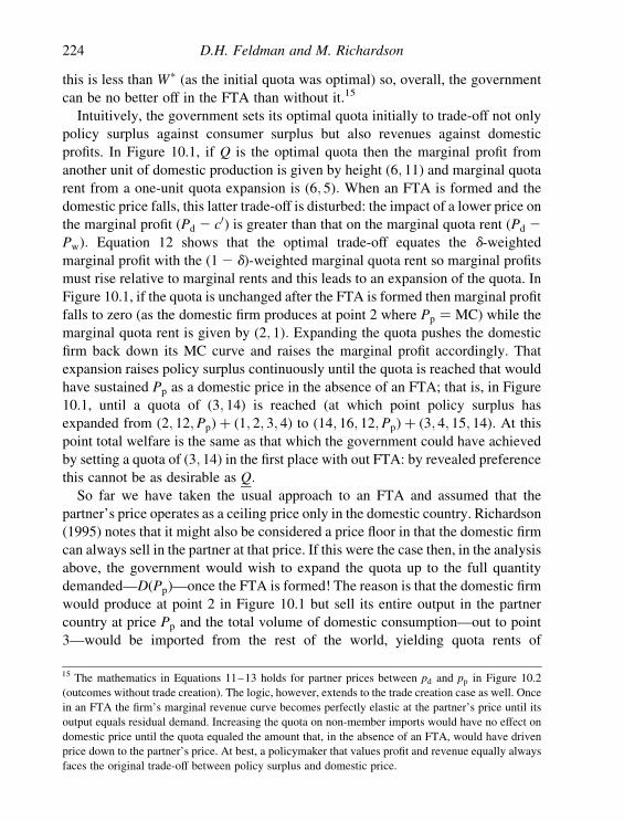
this is less than Wp (as the initial quota was optimal) so, overall, the government

can be no better off in the FTA than without it.15

Intuitively, the government sets its optimal quota initially to trade-off not only

policy surplus against consumer surplus but also revenues against domestic

profits. In Figure 10.1, if Q is the optimal quota then the marginal profit from

another unit of domestic production is given by height ð6; 11Þ and marginal quota

rent from a one-unit quota expansion is ð6; 5Þ: When an FTA is formed and the

domestic price falls, this latter trade-off is disturbed: the impact of a lower price on

the marginal profit ðPd 2 c0Þ is greater than that on the marginal quota rent ðPd 2

PwÞ: Equation 12 shows that the optimal trade-off equates the d-weightedmarginal profit with the ð12 dÞ-weighted marginal quota rent so marginal profits

must rise relative to marginal rents and this leads to an expansion of the quota. In

Figure 10.1, if the quota is unchanged after the FTA is formed then marginal profit

falls to zero (as the domestic firm produces at point 2 where Pp ¼ MC) while the

marginal quota rent is given by ð2; 1Þ: Expanding the quota pushes the domestic

firm back down its MC curve and raises the marginal profit accordingly. That

expansion raises policy surplus continuously until the quota is reached that would

have sustained Pp as a domestic price in the absence of an FTA; that is, in Figure

10.1, until a quota of ð3; 14Þ is reached (at which point policy surplus has

expanded from ð2; 12;PpÞ þ ð1; 2; 3; 4Þ to ð14; 16; 12;PpÞ þ ð3; 4; 15; 14Þ: At thispoint total welfare is the same as that which the government could have achieved

by setting a quota of ð3; 14Þ in the first place with out FTA: by revealed preferencethis cannot be as desirable as Q:

So far we have taken the usual approach to an FTA and assumed that the

partner’s price operates as a ceiling price only in the domestic country. Richardson

(1995) notes that it might also be considered a price floor in that the domestic firm

can always sell in the partner at that price. If this were the case then, in the analysis

above, the government would wish to expand the quota up to the full quantity

demanded—DðPpÞ—once the FTA is formed! The reason is that the domestic firm

would produce at point 2 in Figure 10.1 but sell its entire output in the partner

country at price Pp and the total volume of domestic consumption—out to point

3—would be imported from the rest of the world, yielding quota rents of

15 The mathematics in Equations 11–13 holds for partner prices between pd and pp in Figure 10.2

(outcomes without trade creation). The logic, however, extends to the trade creation case as well. Once

in an FTA the firm’s marginal revenue curve becomes perfectly elastic at the partner’s price until its

output equals residual demand. Increasing the quota on non-member imports would have no effect on

domestic price until the quota equaled the amount that, in the absence of an FTA, would have driven

price down to the partner’s price. At best, a policymaker that values profit and revenue equally always

faces the original trade-off between policy surplus and domestic price.


ð3; 4;Pw;PpÞ: In this case the FTA is clearly desirable even for a government that

weighs revenue and profit equally.

10.3.2. FTA can only be politically attractive if profits are more

highly valued than revenues

Returning to the case where the FTA provides a price ceiling and not a floor, is it

possible that an FTA could be attractive to a government that did not weigh

revenue and profits equally? This could only be the case if an FTA can offer a

trade-off that is not otherwise available, and in this section we identify exactly

such a tradeoff. Consider Figure 10.1 and suppose that the optimal quota, in the

absence of FTA, was ð3; 14Þ: This yields a domestic price of Pp; correspondingconsumer surplus, domestic profits of ð12; 16; 14;PpÞ and quota rents of

ð3; 4; 15; 14Þ: If the home economy joins an FTA with a partner whose price is

Pp and the initial quota is maintained, then the FTA will have no effect. If the

quota is tightened, however, domestic price will not change but domestic output

will increase along the MC curve potentially as far as point 2. With a quota of Q;for instance, the FTA gives profits of ð2; 12;PpÞ and rents of ð1; 2; 3; 4Þ; as we havenoted earlier. The important point here is that profits are higher under the price-

equivalent FTA and appropriate quota than under a quota alone, even though the

sum of revenue and profits is lower. Accordingly, one would anticipate that

joining an FTA might be more attractive to a government that values profits over

revenues. Of course, the FTA will reduce profit if the partner’s price is too low,

which also suggests that the FTA is more likely to be attractive when the partner’s

price is “close” to the pre-FTA domestic price.

To answer this question more generally we must compare welfare levels

between two discretely different regimes: an optimally chosen quota alone, and

an FTA with an optimally adjusted quota. This is intractable even in this simple

model so we turn to some numerical simulations to illustrate the intuitive results

suggested above. We simulate a linear version of the model above in which

Pd ¼ a2 bQ; w½r;P� ¼ bCSðPdÞ þ ð12 bÞr; rðp;RÞ ¼ dpþ ð12 dÞR and

MCðqÞ ¼ aþ gq for constants a; b; b; d; a and g: We confine our attention

to cases in which a quota is initially preferred to a tariff (in the absence of an

FTA). In this setting we can show that the optimal quota when an FTA is joined

(given that domestic production remains positive) is given by

QFTA

¼1

bdg½dðgþ bÞða2 PpÞ þ bð12 dÞðPp 2 PwÞ2 bdða2 aÞ� ð14Þ


We can also calculate the maximum value of this FTA quota such that

the domestic price is exactly Pp—this is the equivalent of the quota ð3; 14Þ inFigure 10.1:

Qmax

¼1

bðgþ bÞ½ðgþ bÞða2 PpÞ þ bða2 PpÞ� ð15Þ

Following our earlier reasoning, if QFTA. Qmax it must be true that the FTA is

politically undesirable: the welfare level achieved at Qmax was attainable in the

absence of the FTA by setting Q ¼ Qmax: But if the quota in the FTA exceeds

Qmax then domestic price will be affected and the FTA is redundant. Again,

whatever welfare is achieved at such a QFTA must have been attainable in the

absence of an FTA and so, by revealed preference, such an FTA cannot be

politically attractive. Thus a necessary condition for an FTA to be politically

attractive is that QFTA, Qmax: This condition can be manipulated as follows:

dg½bða2 PpÞ þ ðgþ bÞða2 PpÞ�

. ðgþ bÞ½bð12 dÞðPp 2 PwÞ þ dðgþ bÞða2 PpÞ2 bdða2 aÞ�

, dgbða2 PpÞ . ðgþ bÞdðgþ b2 gÞða2 PpÞ

þ bð12 dÞðgþ bÞðPp 2 PwÞ2 bdðgþ bÞða2 aÞ

, dgða2 PpÞ . ðgþ bÞ{dða2 PpÞ þ ð12 dÞðPp 2 PwÞ2 dða2 aÞ}

, ðdg2 dðgþ bÞÞða2 PpÞ . ðgþ bÞð12 dÞðPp 2 PwÞ

, dbðPp 2 aÞ . ðgþ bÞð12 dÞðPp 2 PwÞ ð16Þ

This is a necessary condition only, so if Equation 16 does not hold then an FTA

cannot be politically attractive, and this is more likely for low values of d:Turning to the results of the simulations, our earlier intuitions are indeed borne

out. Figure 10.2 shows the difference in welfare in the FTA and without it as d andPp are varied.16 The partner’s price is varied between a; the minimum marginal

cost of the domestic firm, and Pd; the domestic price without an FTA and is

reported as a percentage of that difference. The figure shows that the FTA

becomes less attractive as the partner’s price gets further from the initial price

without the FTA, for most values of d: Further, the FTA is only preferred when dis sufficiently high—in this case above 0.54 or so—and Pp is also high. Also, the

FTA is more likely to be attractive the lower is b; the relative weight the

government places on consumer surplus. This, too, is intuitive. As we suggested

16 The simulations reported here were run using the following parameter values: a ¼ 150; b ¼ 2;

b ¼ 0:1; Pw ¼ a ¼ 25 and g ¼ 0:3: More details are available from the authors on request.


earlier, an FTA will only be attractive if it offers a trade-off that is otherwise

unavailable, and what it offers is the ability to increase profits, at any given price,

beyond that which is achievable without an FTA. When b is high the initial

optimal quota is also high, so the domestic price is low. If this price is less than athere is no domestic production at all and an FTA is redundant.

Interestingly, when b is high an increase in d is likely to lead to an expanded

quota. The reason is that when d is low a quota will be imposed to earn quota rents

which are relatively highly valued. This comes largely at the expense of consumer

surplus. As d rises, however, and profits become more valued relative to rents, the

cost of a quota in terms of foregone consumer surplus becomes more acute since

Figure 10.2: Excess of welfare in FTA over initial welfare, with optimal quotas.


the marginal effect on profits of a tighter quota is smaller than its effect on rents

(given MC . Pw). So, for high b; the attractiveness of a quota to raise profits is

less than its attractiveness to raise quota rents, in a sense, and as profits become

more valued (d rises) so the government finds it more attractive simply to

liberalize the quota entirely.

Our simulations also show that the quota may be either liberalized or tightened

when the FTA is formed. Figure 10.3 illustrates the increase in imports in the FTA

compared to no FTA, when the quota is set optimally in each case. It suggests that

the quota is more likely to be tightened when d is low. Note that for high d and Pp

the policy-maker chooses a prohibitive quota in this setting both within an FTA

and in its absence, hence the difference in imports shown in Figure 10.3 is zero in

Figure 10.3: Excess of optimal quota in FTA over initial optimal quota.


those cases. Figure 10.3 also suggests that, for given d; the quota is more likely to

be tightened when the partner’s price is high. This contradicts with Richardson’s

(1993) tariff-protected competitive industry where joining an FTA leads to an

incentive to liberalize tariffs against non-members.

Lastly, the new political equilibrium will never lead to trade creation in this

industry, so long as quota rents are valued at all. The only case in which it might

appear to is where the residual demand curve (D0 in Figure 10.1) in the post-FTA

political equilibrium intersects the marginal cost curve above the partner’s price.

In that case, the domestic firm would produce to where MC ¼ Pp and this output

plus the quota would be less than demand at the price Pp: However, such a

situation could not reflect an optimal quota as the quota could be expanded with no

consequence for domestic price (and hence consumer surplus) or for domestic

profits. Such an expansion, however, would increase quota rents.

10.4. CONCLUSIONS

This chapter has evaluated the positive and political-economy consequences of

FTA formation for a small domestic economy with quota-protected single-firm

industries. In contrast to the competitive case, FTA formation will not create trade

in the single-firm case when the quota is chosen optimally (and may not create

trade even for an arbitrary quota). Nevertheless, an FTA must prove welfare

enhancing in the traditional sense of increasing real national income. Although the

FTA may worsen domestic overproduction relative to the first best optimum (free

trade) the reduction in consumption deadweight loss unambiguously dominates

any extra production loss.

Conventional welfare gains rarely motivate discriminatory liberalization. We

use a political-support function in which the firm’s profits and quota rents are

substitutable to the policymaker tomake three points. First, for an FTA to dominate

the initial quota-distorted equilibrium, the weight on profit must exceed the weight

on revenue in the policymaker welfare function. Second, politically feasible FTAs

require a partner price close to the initial domestic price. Partner prices closer to that

of the low cost producer cost too much political support from foregone profits and

revenues to justify the lower consumer price. Lastly, moving into an FTA may

create an incentive for the policymaker to liberalize the residual quota on non-

members. Thus, FTA formation need not reduce the volume of world trade outside

of discriminatory regional arrangements. With a quota-protected domestic

monopoly, regional arrangements are neither poison nor panacea.


APPENDIX A

In this section we provide the derivations of Equations 14 and 15 in the chapter:

first, Equation 14 which gives the optimal in-FTA quota in the linear case when

domestic output is positive. The government sets the quota to maximize the

following:

W ¼ bCSþ ð12 bÞr ðA1Þ

where the domestic price is fixed at Pd ¼ Pp thus demand and hence CS is

unchanged as the quota varies. So

dW ¼ ð12 bÞdr ðA2Þ

From the chapter we have

dr

dQFTA¼ d

dp

dQFTAþ ð12 dÞðPp 2 PwÞ

¼ ð12 dÞðPp 2 PwÞ2 dðPp 2 c0Þ ð12Þ

So the optimal quota solves

dr

dQFTA¼ 0 ) c

0¼

1

d{ð12 dÞPw þ ð2d2 1ÞPp} ðA3Þ

Now, in this linear case we have

c0¼ aþ gQ ¼ aþ gðQ2 Q

FTAÞ ) Q

FTA¼ Qþ

1

gða2 c

0Þ ðA4Þ

whereQ is total domestic demand. Substituting Equation A3 into Equation A4 and

simplifying gives

QFTA

¼ QðPpÞ21

dg½ð12 dÞPw 2 da2 ð12 2dÞPp� ðA5Þ

Finally, substituting in forQðPpÞ ¼ ða2 PpÞ=b and simplifying gives Equation 14:

QFTA

¼1

bdg½dðgþ bÞða2 PpÞ þ bð12 dÞðPp 2 PwÞ2 bdða2 aÞ� ð14Þ

What is the maximum value of this FTA quota such that the domestic price is

exactly Pp? To solve this we need to calculate the maximum quota that yields this


price when Pd is not fixed. From Equation 6 of the chapter—the firm’s FOC—we

have

ðQ2 QÞP0d þ Pd 2 c

0¼ 0 ) bQþ a2 2bQ2 ðaþ gðQ2 QÞÞ ¼ 0

) Q ¼ða2 a2 bQÞ

{gþ 2b} ðA6Þ

Substituting this into the inverse demand curve and solving gives the domestic price

as a function of the quota:

p ¼1

{gþ 2b}ððgþ bÞða2 bQÞ þ abÞ ðA7Þ

which can be inverted to find the quota that yields a particular domestic price:

Q ¼1

bðgþ bÞððgþ bÞaþ ab2 ðgþ 2bÞpÞ ðA8Þ

So for p ¼ Pp we have Equation 15 of the chapter:

Qmax

¼1

bðgþ bÞ½ðgþ bÞða2 PpÞ þ bða2 PpÞ� ð15Þ

REFERENCES

Cassing, J. H. and Hillman, A. L. (1985). Political influence motives and the choice

between tariffs and quotas. Journal of International Economics, 19, 279–290.

De Melo, J. and Roland-Holst, D. (1991). “Industrial organization and trade liberalization:

evidence from Korea,” in Empirical Studies of Commercial Policy, R. Baldwin, (ed.),

Chicago: University of Chicago Press, Chapter 10.

Dutz, M. A. (1996). “Oligopolistic firms’ adjustment to quota liberalization,” in Industrial

Evolution in Developing Economies, M. J. Roberts and J. R. Tybout (eds.), Oxford:

Oxford University Press, Chapter 6.

Feldman, D. H. (1993). Redundant tariffs as rational endogenous protection. Economic

Inquiry, 31, 436–447.

Feldman, D. H. (1993). The choice between tariffs and quotas as the means of protection

under autocracy. North American Review of Economics and Finance, 4, 165–178.


Goodman, D. J. and Kaempfer, W. H. (1993). Free trade area formation with quota

protection. North American Review of Economics and Finance, 4, 157–164.

Helpman, E. (1987). Macroeconomic Effects of Price Controls: The Role of the Market

Structure. NBER Working Paper No. 2434.

Hillman, A. L., Tower, E. and Fishelson, G. (1980). On water in the quota. Canadian

Journal of Economics, 13, 310–317.

Kaempfer, W., McClure, H. and Willett, T. D. (1989). Incremental protection and efficient

political choice between tariffs and quotas. Canadian Journal of Economics, 22,

228–236.

Krishna, K. (1989). Trade restrictions as facilitating practices. Journal of International

Economics, 26, 251–270.

Krishna, K. (1993). Theoretical implications of imperfect competition on quota license

prices and auctions. World Bank Economic Review, 7, 113–136.

Krueger, A. O. (1993). Political Economy of Policy Reform in Developing Countries,

Cambridge: The MIT Press.

Lustig, N. (1992).Mexico: The Remaking of an Economy, Washington, DC: The Brookings

Institution.

Meade, J. E. (1955). The Theory of Customs Unions, Amsterdam: North-Holland.

Ng, F. (1996). A Profile of Tariffs, Para-tariffs, Non-tariff Measures, and Economic Growth

in Developing Countries. World Bank, International Trade Division, International

Economics Department.

Ortiz, G. (1991). “Mexico beyond the debt crisis: toward sustainable growth with price

stability,” in Lessons of Economic Stabilization and its Aftermath, M. Bruno, S. Fischer,

E. Helpman, N. Liviatan and L. Meridor (eds.), Cambridge: MIT Press, Chapter 8.

Richardson, M. (1993). Endogenous protection and trade diversion. Journal of

International Economics, 32, 309–324.

Richardson, M. (1995). Tariff revenue competition in a free trade area. European Economic

Review, 39, 1429–1437.

Sweeney, R., Tower, E. andWillett, T. D. (1977). The ranking of alternative tariff and quota

policies in the presence of domestic monopoly. Journal of International Economics, 7,

349–362.

Tybout, J. (2000). Manufacturing firms in developing countries: how well do they do and

why? Journal of Economic Literature, 38, 11–44.

Vousden, N. (1990). The Economics of Trade Protection, Cambridge: Cambridge

University Press.

Whitworth, A. (1980). Monopoly and the case for price controls. Journal of Development

Studies, 17, 80–95.

World Bank (1994). Adjustment in Africa: Reforms, Results, and the Road Ahead.

New York: Oxford University Press.

Young, L. and Anderson, J. (1980). The optimal policies for restricting trade under

uncertainty. Review of Economic Studies, 47, 927–932.

Young, L. and Anderson, J. (1982). Risk aversion and optimal trade restrictions. Review of

Economic Studies, 49, 291–305.


CHAPTER 11

The Political Economy of Trade

Sanctions Against South Africa:

A Gravity Model Approach

WILLIAM H. KAEMPFER* and MARTIN ROSS

Department of Economics, Box 256, University of Colorado at Boulder,

Boulder, CO 80309-0256, USA

Abstract

South African trade fell dramatically during the mid-1980s with the application of

anti-apartheid sanctions that partially restricted trade. This chapter develops the

hypothesis that the severity of sanctions is inversely related to the cost of imposing

those sanctions—a law of demand for sanctions consistent with public choice

principles. We estimate a gravity model of trade flows as a function of distance

and economic mass for South Africa. The results show that sanctions were more

restrictive where trade was less important to a country due to its relative size or

distance from South Africa.

Keywords: South Africa, trade sanctions, gravity model, political economy, public

choice

JEL classification: F1



11.1. INTRODUCTION: THE LAW OF DEMAND FOR SANCTIONS

International economic sanctions are a policy tool employed by one government,

or set of governments, in an attempt to persuade another sovereign state to change

some objectionable policy. One implication of sanctions policy, however, is that

not only do the sanctions impose economic (and presumably political) costs on the

target country, they can also be costly to the sending country. In particular,

sanctions can be thought of as a policy funded by an implicit tax that falls

disproportionately on a subset of specific interests in the sending country—

namely those entities with trading interests in the target (Kaempfer and

Lowenberg, 1990, 1992).

Interest group models in public choice theory suggest that an interest is able to

attain government policy objectives only to the extent that its willingness and

effectiveness to pressure for some policy exceeds the willingness and

effectiveness of the other, contrary interests to object to and block the policy

initiative (Becker, 1985). To this end, one can infer that as economic sanctions

impose a rising policy cost upon some set of negatively impacted interests, then

those sanctions will not be as severe. That is, there should be a negatively sloped

demand curve for sanctions. In many applications of sanctions, however, the

domestic costs of an embargo are weighed against having no costly sanctions at

all. In other words, the potential imposition of sanctions can be seen as a

dichotomous policy choice in which either a total trade embargo is applied (e.g.,

Iraq and Cuba), or negligible, low-cost sanctions are applied such as cancellation

of cultural or sport exchanges. Along these lines, Bonetti (1997) finds that the

probability of imposing trade sanctions is inversely related to the extent of

presanction trade flows between two countries.

One much different case of the imposition of sanctions was that of sanctions

against South Africa’s apartheid regime in the 1980s. Most western countries as

well as the African neighbors of South Africa adopted some form of sanctions

policy against the white regime in South Africa in an attempt to coerce that

government to end political repression of its majority population groups and

democratize. However, a uniform multilateral trade embargo policy was not

adopted. Rather, in this case the political process within each trade partner

established some sort of national package of partial sanctions, three features of

which are noteworthy. First, the sanctions policies were internally decided upon

by the sanctioning nations, not by some multi-lateral authority such as the UN or

Organization of Commonwealth States. Second, the sanctions were not uniform

across countries. Third, anti-apartheid sanctions were not a dichotomous policy,

but instead a variety of specific goods categories were embargoed in various

countries (Kaempfer and Lowenberg, 1989). As a result, sanctions against

W.H. Kaempfer and M. Ross234

South Africa allow the opportunity to test the proposition that as the cost of

sanctions rises, less severe sanctions will be imposed.

In this chapter, we undertake such a test by means of applying a gravity model

to South African trade before and after the time of the major imposition of

sanctions in 1986. Gravity models (see, for instance, Bergstrand, 1985) explain

trade as a function of mass and distance where greater economic mass (i.e., GDP

and/or per capita GDP) and geographic closeness (i.e., lower transport costs) will

lead to a greater volume of trade between countries. For the purposes of our point,

those same attractors—mass and closeness—raise the political costs of applying

sanctions. Consequently, we expect to find that the trade for which there is the

least “gravitational attraction” will be the most impacted by sanctions, and

consequently we hypothesize that the gravity model will explain South African

trade better in the late 1980s relative to the early 1980s. This hypothesis is also

tested by examining changes in the effects of geographical proximity over time.

11.2. SOUTH AFRICAN TRADE DURING THE 1980S

South Africa’s economy in the 1980s, while largely mineral based, had a number

of unusual features. Decades of apartheid-induced partial isolationism led the

country to have a number of large parastatal economic entities that were not

particularly economically efficient. However, a relatively large upper income

group led to a great deal of imports from other high-income countries, especially

in manufactured goods. At the same time, beyond the mining section, a

manufacturing sector in South Africa served some export markets, and a southern

hemisphere location allowed for “off-season” agricultural exports of fruits and

vegetables. Overall, the volume of trade (imports and exports) amounted to 60%

of GDP in 1981. This relatively large proportion of trade in the economy provided

a vehicle for other nations to alter the behavior of the South African government.

The 1986 anti-apartheid sanctions against South Africa were imposed by

several important trading partners, including the United States, United Kingdom,

European Economic Community, Canada and other Commonwealth countries and

Japan. The sanctions involved areas such as disinvestments, bank loans, tourism

restrictions, and import and export restrictions. The focus here is on the trading

restrictions, the majority of which involved restricting South Africa’s exports to

one or more of its trading partners—specifically of steel, iron, coal, uranium,

textiles, Krugerrands and agricultural products, as well as some limited imports

generally in the areas of arms and technology goods.

Complete data series are only available for three African countries (Kenya,

Malawi and Zimbabwe). These nations are the three largest African trading

Political Economy of Trade Sanctions Against South Africa 235

partners of South Africa and are relatively close geographically to South Africa.

Data for the top 14 non-African trading partners are also examined and show the

trading trends with the rest of the world (ROW). (Note: in the early 1980s, Sweden

had a large trade volume with South Africa. However, as a strong supporter of the

sanctions, their trade after 1986 declined to the point where it is difficult to obtain

the exact values.)

Figure 11.1 shows the aggregate trade, imports and exports of South Africa with

the three African countries and the 14 other countries (ROW). Values are in 1985

South African Rand. Figure 11.2 presents the figures with the individual African

nations, while Figures 11.3–11.6 give the trade amounts for the remaining 14

Figure 11.1:


Figure 11.2:


included nations. There is a large variation in the relative sizes of the illustrated

trade flows—the US is the largest, followed by Germany, Japan and the United

Kingdom.

Table 11.1 summarizes the information on trade which is presented in the

figures. The table shows the percentage changes in trade from 1981 to 1985 and

from 1986 to 1990 (where the denominator used in calculating the percentage

changes in both columns in the table is the value of trade in 1981). These values

show that South Africa’s trade with the world as a whole was declining

significantly from 1981 to 1985.

11.3. THE GRAVITY MODEL OF TRADE

Since their development, gravity models have been empirically successful at

explaining the volume of trade flows between countries. Tinbergen (1962) and

Poyhonen (1963) were the first to propose these econometric models of bilateral

trade. The models explained the volume of trade between two countries

Figure 11.3:


as a function of their GNPs and the distance between them. The GNP variable

represents the economic mass of a country and thus the cumulative income

elasticity impact on trade, while distance is a proxy for transport costs. Linnemann

(1966) included a population variable in the analysis to account for scale

economies. Leamer (1974) used this expanded gravity model to test the effects of

factor endowments and other country characteristics on trade flows. While these

models were quite accurate and possessed an intuitive appeal, they lacked a strong

theoretical framework. Bergstrand (1985, 1989) removed some of these concerns

by extending the basic model to include a microeconomic foundation.

This chapter adopts the novel approach of employing the gravity model as a

method of examining the severity of the sanctions against South Africa. The

hypothesis is that the severity of sanctions should be inversely related to cost. The

gravity model predicts that countries close to South Africa or countries with

higher income (either total or per capita) will have more trade with South Africa.

By similar reasoning, these countries will find it more politically costly to restrict

trade via sanctions. Consequently, following the imposition of differential

Figure 11.4:


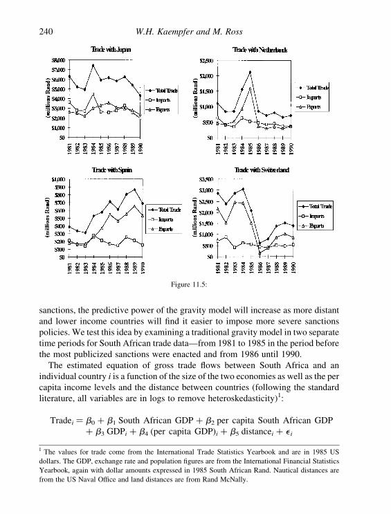
sanctions, the predictive power of the gravity model will increase as more distant

and lower income countries will find it easier to impose more severe sanctions

policies. We test this idea by examining a traditional gravity model in two separate

time periods for South African trade data—from 1981 to 1985 in the period before

the most publicized sanctions were enacted and from 1986 until 1990.

The estimated equation of gross trade flows between South Africa and an

individual country i is a function of the size of the two economies as well as the per

capita income levels and the distance between countries (following the standard

literature, all variables are in logs to remove heteroskedasticity)1:

Tradei ¼ b0 þ b1 South African GDP þ b2 per capita South African GDP

þ b3 GDPi þ b4 (per capita GDP)i þ b5 distancei þ e i

Figure 11.5:

1 The values for trade come from the International Trade Statistics Yearbook and are in 1985 US

dollars. The GDP, exchange rate and population figures are from the International Financial Statistics

Yearbook, again with dollar amounts expressed in 1985 South African Rand. Nautical distances are

from the US Naval Office and land distances are from Rand McNally.


The effect of sanctions may be captured in two ways. First, the gravity equation

may explain a different proportion of the variation in trade flows across the two

time periods. Second, there may be a significant difference between the parameter

estimates of the distance and foreign income variable before and after sanctions.

11.4. EMPIRICAL RESULTS

Table 11.2 presents the regression results, where the parameter estimates indicate

elasticities. The gravity equation does a fairly good job of predicting the trade

Figure 11.6:


flows between South Africa and the ROW. While the GDP variables for the

trading partners of South Africa are significant, South African GDP and per capita

GDP are not. This may be due to the relatively large amount of trade in the South

African economy and the small variation in these variables over the sample.

Table 11.1: Percentage changes in trade with South Africa.

1981–1985 1986–1990 1981–1990

Africa 217 24 220

ROW 24 217 220

Kenya 158 278 80

Malawi 58 228 30

Zimbabwe 230 1 230

Australia 28 272 244

Austria 211 64 53

Belgium 13 19 32

Canada 230 220 250

France 224 25 229

Germany 0 5 6

Israel 75 212 63

Italy 6 23 3

Japan 26 225 231

The Netherlands 93 2127 234

Spain 49 29 78

Switzerland 228 224 251

United Kingdom 29 27 215

United States 28 231 240

Table 11.2: Regression results (dependent variable is trade with country i).

Variable 1981–1985 1986–1990

Constant 3.96 (0.06) 17.23 (0.62)

South African GDP 20.18 (20.01) 21.38 (20.28)

Per capita South African GDP 0.17 (0.01) 0.42 (0.11)

GDPi 0.87* (7.56) 0.60* (6.56)

(Per capita GDP)i 0.03 (0.17) 0.54* (3.69)

Distancei 20.89* (24.70) 21.30* (27.57)

F-statistic 22.16 39.25

R2 0.58 0.71

Adjusted R2 0.56 0.70

t-statistics in parentheses. *significance at the 1% level.


The gravity model states that a country’s trade with a close, large, high-income

country will be greater than trade flows to a distant, small, low-income country.

However, the application of sanctions by a close, large, high-income country will

be more costly to that country due to the greater amount of trade that country had

initially with its trading partner. Many factors explain the volume of trade between

two nations. However, after the sanctions are enacted, the estimated importance of

economic mass and proximity may increase since sanctions may tend to be less

restrictive where trade is important. These political costs of applying sanctions

should lead to an increase in the predictive power of the gravity model after

sanctions take effect.

The adjusted R2 is 0.56 for the time period 1981–1985 and 0.70 for 1986–

1990. A comparison of these two values indicates that the gravity model explains

more of the variation in trade after the sanctions takes effect. This suggests that the

sanctions were more restrictive where trade was less important and implies the law

of demand for sanctions.

Another indication of the downward sloping demand for sanctions comes

from comparing the parameter estimates on the distance and foreign GDP

variables in the two estimated equations. After 1986, if the predictive power of

the gravity model is improved, then the influence of distance and GDP on trade

should increase since the most restrictive sanctions should occur where

restricted trade with South Africa is least costly. The results in Table 11.2 show

that the effect of the distance variable is more negative from 1986 to 1990 than

it is from 1981 to 1985. A t-test shows that there is a significant difference

between the two estimates. The results show that the increasing distance has a

significantly more negative effect on trade after the sanctions took effect.

Similarly, when taken together, the two foreign income variables show a greater

positive effect on trade after the sanctions. The coefficient on foreign GDP

declines slightly, though not significantly, between the two estimated equations,

while the foreign per capita GDP variable only becomes significantly positive

in the second time period.


The use of trade sanctions imposes costs not only upon the target of those

sanctions but also on the sanctioning countries as well. Ceteris paribus, the costs

of imposing sanctions will rise as the trade linkages between sender and target

rise. Furthermore, these costs are likely to have a political manifestation that will

make severe sanctions more difficult to impose when sanctions costs are high on

the sending nation.


In this chapter, we examined South African trade during the 1980s, a period of

great sanctions turbulence, by means of a gravity model. Our results support the

hypothesis that the post sanctions trade interruptions increase the explanatory

power of the gravity model. This suggests, in accordance with public choice

principles, that sanctions against South Africa were most severe where

interruptions of trade with South Africa were least costly.

ACKNOWLEDGEMENTS

We are grateful to Ed Tower and Ed Balistreri for their help. Tony Lowenberg’s

advice and guidance was invaluable.

REFERENCES

Becker, G. (1985). Public policies, pressure groups, and dead weight costs. Journal of

Public Economics, 28, 329–347.

Bergstrand, J. (1985). The gravity equation in international trade: some microeconomic

foundations and empirical evidence. Review of Economics and Statistics, 67,

474–481.

Bergstrand, J. (1989). The generalized gravity equation, monopolistic competition, and the

factor-proportions theory in international trade. Review of Economics and Statistics, 71,

143–153.

Bonetti, S. (1997). A test of the public choice theory of economic sanctions. Applied

Economics Letters, 4, 729–732.

International Financial Statistics Yearbook, International Monetary Fund, various years.

International Trade Statistics Yearbook, International Monetary Fund, various years.

Kaempfer, W. and Lowenberg, A. (1989). Sanctioning South Africa: the politics behind the

policies. Cato Journal, 8, 713–727.

Kaempfer, W. and Lowenberg, A. (1990). “Analyzing economic sanctions: toward

a public choice framework,” in International Trade Policies: Gains from Exchange

between Economics and Political Science, Studies in International Trade Policies, T.

Willett and J. Odell (eds.), Ann Arbor, MI: University of Michigan Press, 173–193.

Kaempfer, W. and Lowenberg, A. (1992). International Economic Sanctions: A Public

Choice Perspective, Boulder, CO: Westview Press.

Leamer, E. (1974). The commodity composition of international trade in manufactures: an

empirical analysis. Oxford Economic Papers, 350–374.

Linnemann, H. (1966). An Economic Study of International Trade Flows, Amsterdam:

North-Holland.


Poyhonen, P. (1963). A tentative model for the volume of trade between countries.

Welwirtschaftliches Archiv, 90, 93–99.

Rand McNally Atlas, Rand McNally and Co.

Tinbergen, J. (1962). Shaping the World Economy: Suggestions for an International

Economic Policy, New York: McGraw-Hill.

US Naval Oceanographic Office. Distance Between Ports, H.O. Publication No. 151. US

Government Printing Office.


PART IV

Aid and Foreign Investment Policies

CHAPTER 12

The Political Economy of

Unconditional and Conditional Foreign

Assistance: Grants vs. Loan Rollovers

WOLFGANG MAYERa,* and ALEX MOURMOURASb

aDepartment of Economics, University of Cincinnati, Cincinnati, OH 45221-0371, USAbIMF Institute, International Monetary Fund, Washington, DC 20431, USA

Abstract

Improving the effectiveness of assistance programs is a priority of international

financial institutions (IFIs). This chapter examines the effectiveness of alternative

assistance instruments in a dynamic political-economy framework. Economic

policies of the receiving country are distorted by the influence of a domestic

interest group. The assistance-providing IFI aims at reducing these distortions.

The IFI provides assistance either as grants or loans, and either conditionally on

reducing policy distortions or unconditionally. The chapter shows that, other

things constant, one-time grants are more effective than loan rollovers when

assistance is unconditional, but that this effectiveness ranking is reversed when

assistance is conditional.

Keywords: International Monetary Fund, conditionality, common agency models,

grants vs. loans

JEL classifications: E61, F33, F34



12.1. INTRODUCTION

Developing countries have received large amounts of international financial

assistance over the last 50 years. Much of this assistance has been channeled from

developed to developing countries under the auspices of International Financial

Institutions (IFIs). In some instances, resource transfers have had lasting benefits

to the recipient countries. In many other cases, however, enduring success has

eluded successive IFI-supported economic reform programs. Hence, it comes as

no surprise that IFIs have considered redesigning their assistance programs to

achieve better results. A general goal of this chapter is to gain new insights about

the effectiveness of different forms of assistance.

Two important policy concerns in the design of IFI-supported programs are the

length of IFI financial involvement in recipient countries and its “payback

provisions.” Specifically, at issue is whether assistance ought to continue in the

form of (often concessional) loans or whether it ought to be converted to grants

that do not have to be repaid. The length of IFI financial involvement has a direct

bearing on the issue of inappropriate “prolonged use” of IFI resources. Prolonged

users are transition or developing countries whose economic reform and

adjustment programs have been supported extensively by the IFIs through

successions of conditional loans that have often spanned two or more decades.1

While prolonged financial association with IFIs has in some cases been beneficial

to low-income developing and transition countries, in other cases the succession

of low-interest IFI loans has failed to yield lasting improvements in policies and

economic performance.2 Better ex post monitoring of reform programs with

identified prolonged users and graduation or “exit” from financial engagement in

cases of inappropriate prolonged use is now an explicit IFI goal.3

The repayment terms of assistance are a second major policy issue in the

design of both bilateral and multilateral assistance programs. Several decades

ago, Friedman (1958, p. 515) proposed to substantially increase US

development assistance and turn it into a “final terminal grant…[that] should

be something like two to three times the annual grants we have been making to

the country.” This issue of grants vs. loans resurfaced again recently after US

President George W. Bush proposed to turn into grants one half of the

assistance provided through the International Development Association (IDA),

1 See IMF (2002) for a detailed definition of prolonged use and for the list of countries identified as

prolonged users of IMF resources.2 Bird et al. (2000) and IMF (2002, 2003a) contain detailed discussions of the drawbacks of prolonged

use. IMF (2003b) offers guidance on how to avoid inappropriate prolonged use of IMF resources.3 See, for instance, IMF (2002, p. 328).

W. Mayer and A. Mourmouras250

the arm of the World Bank that provides assistance to qualified low-income

countries. While the World Bank welcomed the proposal, it was met with fierce

resistance elsewhere. Some bilateral donors expressed concerns that, in the

absence of additional funds to replenish its capital, a switch to grants would

deplete IDA capital and compromise its ability to provide assistance to poor

countries in the future. Eventually the G-7 agreed in a June 2002 meeting of

their finance ministers in Halifax to increase the proportion of IDA funding that

is provided in the form of grants to between 18–21%, as Cunningham (2002)

points out.

This chapter assesses the merits of different forms of IFI financial involvement,

including their length and repayment terms (whether grants or loans), with the

help of a dynamic version of the political-economy model developed by Mayer

and Mourmouras (2002). They apply the common agency framework of

Grossman and Helpman (1994) and Dixit et al. (1997) to study the effects of

conditional IFI assistance programs in the presence of domestic interest groups.

Interest groups resist reforms when their privileges (rents) are impaired by the

implementation of efficiency-enhancing policy measures. The IFI uses its

financial leverage to steer member governments toward policies that promote

domestic and international prosperity, an assumption that is consistent with the

IFIs’ stated purposes.4 For assistance programs to succeed, IFIs must fully account

for the influence of domestic interest groups on the policy choices of assistance-

receiving governments. IFI assistance helps shift the political equilibrium in

recipient countries and improve the quality of policies selected, thus providing

a countervailing influence to the power of domestic special interests.5

In this framework, we compare a one-time “final” grant with a succession of

one-period IFI loans of the same size that, for simplicity, are assumed to be

interest-free. Whereas the grant cannot be recalled once its conditionality is met

and the IFI has released its funds, assistance that takes the form of loans can be cut

off (not be renewed) if the recipient government does not adhere to the agreed

conditions. The effectiveness of assistance is judged from the IFI’s point of view.

The IFI acts on behalf of the world community, with the objective of maximizing

world welfare. It can raise world welfare in two ways: one is to transfer resources

from the rest of the world (ROW) to the developing country; the other is to create

4 See, for instance, the IMF’s Articles of Agreement, especially Article I, Section 5.5 The experience with reforms in some countries of the Commonwealth of Independent States in the

1990s is a particularly good example of the resistance of special interests to reforms. During the early

years of transition, “red directors” and other special interests used their political influence to evade

taxes, obtain subsidies, strip the assets on state enterprises and extract other special privileges. The IFIs

provided assistance to pro-reform governments while being aware of the need of reformers to stay in

power.

Unconditional and Conditional Foreign Assistance 251

incentives for the assistance-receiving country to reduce its policy-created

distortions. The developing country’s incumbent government chooses economic

policies under the influence of a domestic interest group. Its objective is to

maximize political support that comes from both the interest group and the general

public.

An advantage of assistance through loan rollovers is that the IFI can adjust

its assistance package as economic and political circumstances change over

time. The amount of a loan depends on its benefit in the receiving country and

its cost to the ROW, as well as on the recipient government’s concern for its

general public. If, at time of repayment, any of these influences has changed,

the IFI can replace the repaid loan with a new one that differs in size. Should all

economic and political parameters remain unchanged, the IFI’s interests are best

served by simply reissuing the repaid loan. A grant, on the other hand, cannot

be adjusted ex post. Once made, all transferred resources are permanently

shifted from the ROW to the developing country. No matter how the IFI’s

incentives to support a developing country might have changed, the grant

cannot be recalled.

An advantage of assistance through a grant is that the set of projects for which

transferred resources can be employed is larger than for loans. The need to repay

a loan after a specified time interval limits loan-financed investments to short-

term projects. Knowing that assistance through grants cannot be reversed, on the

other hand, enables the receiving country to invest in both short- and long-term

projects.

The specific purpose of this chapter is to highlight the implications of a third

difference between loan rollovers and a one-time “final” grant, namely, of their

“commitment value”. The interactions between an aid-providing IFI, an aid-

receiving government, and an interest group unfold in a multi-period game.

Assistance through loans can be periodically revised; assistance through grants

cannot. Accordingly, the grant represents a stronger commitment on the part of the

IFI. At issue is whether this difference in commitment value introduces a bias in

favor of either the policy of loan rollovers or a one-time grant, judged from the

perspective of the assistance-giving IFI. Stated differently, is world welfare higher

when the IFI provides assistance through loan rollovers or through a one-time

grant, assuming away all other advantages and disadvantages of the two

instruments?

Our answer to the above question is clear-cut: the IFI is better off assisting

through a final grant than through loan rollovers when assistance is unconditional;

but the IFI is better off assisting through loan rollovers than a final grant when

assistance is conditional. These conclusions are derived from a model in which the

IFI compares the present value of world welfare resulting from a grant with the


present value of welfare resulting from a succession of loans.6 The model captures

the influence of an interest group on the developing country’s government by

adopting the Dixit et al. (1997) formulation of a truthful equilibrium. The interest-

group-influenced government plays a game with the IFI both when assistance is

unconditional and when it is provided conditionally. When assistance is

unconditional and takes the form of loans that are being rolled over, the

government chooses its economics policies and the IFI chooses its loan at the

same time, namely, at the beginning of each period. In the case of a “final” grant,

the government still chooses its policies at the beginning of each period, but the

IFI can choose the grant value only once, namely, at the beginning of the initial

period.

When assistance is conditional, the nature of the political game changes

dramatically as the IFI joins the interest group as a principal in a common-agency

game. The implications for welfare of the IFI are drawn from the conditions of a

truthful equilibrium. In the case of loan rollovers, government, interest group, and

IFI play a two-stage game at the beginning of each period. The IFI is thus engaged

in a prolonged financial association with the recipient country. In the case of a

grant, on the other hand, the three players engage in a two-stage game only at the

beginning of the initial period. While the IFI accounts for government responses

in succeeding periods, it can act only during the initial period. For all periods

beyond the initial one, only the government and the interest group can take

actions. By definition, the policy of providing a final grant does not lead to a

prolonged financial association between the IFI and the recipient country.

The conclusion that a final grant is superior, from the IFI’s point of view, to an

indefinite rollover of a loan of the same amount is not surprising for the case of

unconditional assistance. The higher commitment value of the one-time grant

conveys a benefit to the IFI. As it chooses the grant level prior to the government’s

choices of policies beyond the initial period, the IFI has some first-mover

advantages in the unconditional assistance game. Under conditional assistance,

loan rollovers are superior to a grant because it enables the IFI to enforce

conditionality in each period. A critical feature of the political equilibrium under

conditional assistance is that it results in Pareto-optimality. The outcome is a

combination of assistance and interest group-influenced economic policies that

maximizes joint welfare of the three players, namely, government, interest group,

and IFI. When assistance takes the form of one-period renewable loans, the IFI’s

ability to enforce its conditions on economic policies assures Pareto-optimality.

6 An alternative political economy model is formulated by Drazen (2002) whose government contends

with veto players; i.e., with constitutional actors that influence policy-making from within the

government.


When assistance takes the form of a one-time grant, on the other hand, the

governmentmust adopt distortion-reducing policies only during the initial period in

order to receive the grant. The IFI’s ability to enforce economic policy conditions

disappears after the initial period, as the grant results in an irreversible transfer of

resources.After the initial period, the grant-receiving government takes the value of

the grant as given and views it the same way as an unconditional grant of the same

value. The choices of assistance by the IFI and economic policies by the

government are then no longer Pareto-optimal. Furthermore, this departure from

Pareto-optimality under a conditional grant, when contrasted to the Pareto-optimal

outcome under conditional loan rollovers, comes at the cost of reduced IFI welfare.

The IFI is worse off under a conditional grant than under conditional loan rollovers.

12.2. THE COMMON AGENCY MODEL

12.2.1. Decision makers and their objectives

Consider a developing country whose economic policies are shaped by the

interactions of three different decision makers. First, an incumbent domestic

government chooses the country’s economic policies. Second, a domestic interest

group that benefits from policies that distort the economy attempts to influence the

policy maker. Third, an IFI that acts as gatekeeper of the world’s welfare provides

economic assistance. This assistance benefits the developing country directly as it

increases its capital stock, as well as indirectly as it lowers the level of economic-

policy-generated distortions.

Welfare of the developing country is measured by its national income. Given

the country’s endowment with labor and capital, national income depends on the

amount of economic assistance received, A; and the degree of economic

distortions generated by economic policies. The economic assistance enables the

country to expand its capital stock. The degree of distortions is measured by an

index 0 # v , 1; and it is assumed that the distortion-caused loss in national

income rises linearly with the distortion index. The developing country’s welfare,

W ; therefore, is

W ¼ ð12 vÞyðAÞ ð1Þ

where yð0Þ measures potential national income in the absence of distortions and

with no assistance, and where y0ðAÞ . 0 and y00ðAÞ , 0 for A $ 0:The incumbent government chooses the economic policies of the developing

country. Its objective is to adopt policies, and a corresponding distortion index v;


to maximize its political support from the country’s interest group and general

public. As in Grossman and Helpman (1994), the government receives political

support from the interest group in the form of financial contributions, C; and fromthe general public in form of “approval”. The latter depends on the country’s

overall welfare, W : In making policy choices, the government faces conflicting

attitudes of interest group and general public; the interest group benefits from

policies that are more distorting—such as tariffs, quotas, monopolies, subsidies,

etc.—while the general public is hurt by distortions. To pursue its goals, the

interest group tenders a financial contribution schedule, CðvÞ; to the government.

This schedule makes the amount of financial support contingent on the

government’s choice of distorting policies that favor the interest group. The

government’s political support function, therefore, is written as

G ¼ CðvÞ þ að12 vÞyðAÞ ð2Þ

where a $ 0 is a parameter that reflects the government’s concern for welfare of

the general public. Its value depends on the government’s dependence on the

goodwill of the public. When the developing country’s political institutions are

weak, the value of a tends to be small.

There is only one interest group in the developing country. It benefits from

certain policies that are distorting and, therefore, pressures the government to adopt

them. The interest group’s net welfare,V; equals utility obtained from the distorting

policies, UðvÞ; minus its financial contribution to the government, CðvÞ; i.e.,

V ¼ UðvÞ2 CðvÞ ð3Þ

where the group’s welfare without contributing is assumed to rise with the

distortion index at a decreasing rate. Hence, U 0ðvÞ . 0 and U 00ðvÞ , 0: We also

assume that limv!0 U0ðvÞ ¼ 1 and limv!1 U

0ðvÞ ¼ 0: These assumptions assure

that the economy is always riddled with distorting policy choices as along as there

is an interest group.

Finally, there exists an international financial institution (IFI). It is an

institution that was set up in the past by the entire world community. Its intended

mission is to serve as a public-interest institution and to maximize world welfare

by channeling assistance from the ROW to a developing country. Welfare of the

ROW is also measured by its national income. In contrast to the developing

country, however, distorting economic policies have a negligible impact on the

ROW’s total output. Given the ROW’s factor endowments, its welfare,Wp; solelydepends on the amount of assistance provided, such that

Wp¼ y

pð2AÞ ð4Þ


where ypð0Þ is the ROW’s output in the absence of assistance, yp0ð2AÞ . 0 and

yp00ð2AÞ , 0 for all A $ 0: Given the welfare measures of the developing country

and ROW, the IFI’s objective function is

I ¼ ð12 vÞyðAÞ þ ypð2AÞ ð5Þ

12.2.2. Political equilibrium with unconditional assistance

The nature of the developing country’s political equilibrium critically depends on

whether the IFI provides assistance conditionally or unconditionally. Assistance is

conditional if the IFI makes the amount of aid contingent on the adoption of

distortion-reducing economic policies. As explained by Mayer and Mourmouras

(2002), the conditional assistance scenario can be conveniently modeled within

the political-economy, common-agency framework of Grossman and Helpman

(1994) and Dixit et al. (1997). The government acts as the common agent of

domestic interest group and IFI. The latter present the government with a

contribution and assistance schedule, respectively, to press for their opposing

interests in economic policies. Assistance is unconditional if its provision by the

IFI is not contingent on the government’s adoption of distortion-reducing policies.

Although the IFI does not impose conditions, it is fully aware that world welfare

depends on the assistance-receiving country’s policy distortions. The IFI,

therefore, reacts to the government’s policy choices even though there is no

contractual agreement between IFI and government. Accordingly, the political

game itself involves only the developing country’s government and its interest

group when assistance is unconditional.

Under unconditional assistance, the government’s choice of policies is the

outcome of a two-stage game in which the government chooses the distortion

index (economic policy) in the second stage given the financial contribution

schedule tendered by the interest group in the first stage. We are focusing on

equilibria that are truthful; i.e., on equilibria for which the contribution schedule of

the interest group is truthful relative to the equilibrium welfare level of the players.

The general conditions for a truthful political equilibrium are stated in Proposition

3 of Dixit et al. (1997). Adapting these conditions to our situation of a political

game in which only one interest group and the government participate, the truthful

political equilibrium consists of a truthful financial contribution schedule, CT; anda distortion index, v0; that is characterized by two conditions: first, the

government’s choice of v0 must be such that v0 ¼ argmax0#v,1 ½CTðv;V0Þ þ

að12 vÞyðAÞ�; where V0 denotes the interest group’s net welfare in equilibrium

and A is the amount of unconditional aid received when there is an interest group.


Second, ½CTðw0;V0Þ þ að12 v0ÞyðAÞ� ¼ að12 v2V ÞyðA2V Þ; where v2V is the

distortion index the government would choose in the absence of influence seeking

by the interest group and A2V is the amount of unconditional aid received in the

absence of an interest group. This second condition states that the interest group’s

truthful contribution is just enough to make political support for the government

the same with influence seeking as it would be without influence seeking. With no

interest group—as expressed by the right-hand side of the equation where C is set

equal to zero—the government would choose distortion-free economic policies

such that v2V ¼ 0 and the IFI would provide A2V of aid to this distortion-free

economy. One also can see from Equation 3 that CTðv;V0Þ ¼ UðvÞ2 V0:Consequently, the first of above conditions requires that v0 is chosen to satisfy

U0ðv0

Þ2 ayðAÞ ¼ 0 ð6Þ

whereas the second condition implies that the interest group’s equilibrium

contribution equals

CTðv0;V0

Þ ¼ a½v0yðAÞ þ yðA

2VÞ2 yðAÞ� ð7Þ

Clearly, the degree of distortions, v0 depends on both the amount of unconditional

assistance received from the IFI, A; and the government’s concern for the general

public’s welfare, a: As can be seen from Equation 6, the more unconditional aid is

received and the more the government cares for the public’s welfare, the less-

distorting policies are adopted. This response of the government to different

assistance levels is traced out in Figure 12.1 as the RGRG curve. Since U 00ð·Þ , 0;the government’s policy reaction curve is downward sloping.

12.2.3. Political equilibrium with conditional assistance

Assistance is conditional when the IFI makes its aid to the developing country

contingent on the government’s adoption of less-distorting policies. The IFI,

thereby, becomes a second principal in the economic-policy game. As before, the

government chooses economic policies and the corresponding distortion index.

But unlike the unconditional assistance scenario, the interest group’s pressure for

more-distorting policies is now counteracted by the IFI that, in the interest of

world welfare, pushes for less-distorting policies. We now add an assistance

schedule tendered by the IFI to the contribution schedule of the interest group.

Although both payment schedules are offered to the government, an important

difference between them is that interest group contributions raise the govern-

ment’s political support directly whereas assistance payments benefit the


government only indirectly. The interest group contribution goes into the

campaign funds or personal pockets of politicians that constitute the government.

The assistance payment, on the other hand, goes in its entirety to expand the

economy’s production potential. The raised production potential enlarges national

income that, in turn, leads to stronger approval of the government by the general

public.

The conditional assistance model again adopts the common-agency approach

first developed by Bernheim and Whinston (1986) and later applied and further

refined by Grossman and Helpman (1994) and Dixit et al. (1997). The government

is viewed as the common agent of interest group and IFI. They play a two-stage

economic-policy game in which the government chooses policies in the second

stage given the contribution schedule of the interest group and the assistance

schedule of the IFI. Both payment schedules are offered to the government in the

first stage. Again we are in search of an equilibrium in which both contribution

schedule, CT; and assistance schedule, AT; are truthful. And again we employ the

conditions of Proposition 3 of Dixit et al. (1997) to characterize this truthful

equilibrium. The first condition now is that the government’s policy choice, v1; issuch that v1 ¼ argmax0#v,1 {C

Tðv;V1Þ þ að12 vÞy½ATðv; I1Þ�}; where V1 and

I1; respectively, denote the interest group’s net welfare and the entire world’s

(IFI’s) welfare evaluated at the conditional assistance equilibrium. Second, the

Figure 12.1: Conditional assistance equilibrium.


truthful contribution schedule of the interest group in equilibrium must satisfy

{CTðv1;V1Þ þ að12 v1Þy½ATðv1; I1Þ�} ¼ að12 v2V Þy½ATðv2V ; I1Þ�; where

v2V is again the government’s choice of the distortion index when the interest

group does not contribute. As was the case in the unconditional assistance model,

v2V ¼ 0: Third, the truthful assistance schedule of the IFI must satisfy

{C T(v 1,V 1) þ a(1 2 v 1)y[A T(v 1, I 1)]} ¼ {C T(v 2I,V 1) þ a(1 2 v 2I)y(0)},

where v2I. 0 would be the government’s choice of the distortion index if the IFI

did not offer any conditional assistance. The first condition states that the

government chooses a policy that, given the truthful contribution schedule of the

interest group and the truthful assistance schedule of the IFI, maximizes its

political support. The second and third conditions spell out how much interest

group and IFI, respectively, contribute. The interest group’s truthful equilibrium

contribution must be such that political support for the government is as strong

when it contributes as it would be if it did not contribute, whereby the

government-adopted policies entail distortion index v2V ¼ 0 and the IFI is just as

well off as in equilibrium. The IFI’s truthful equilibrium assistance payment must

be such that political support for the government is as strong when the IFI assists

as it would be if it made no conditional assistance payment, whereby the

government chooses distortion index v2I ; and the interest group is just as well offas in equilibrium.

Recalling again that CTðv;V1Þ ¼ UðvÞ2 V1; the first condition for a truthful

equilibrium requires that v1 is chosen such that

2U 0ðv1Þ2 ay½ATðv1; I1Þ�

að12 v1Þy0½ATðv1; I1Þ�¼

2y½ATðv1; I1Þ�

yp 0½2ATðv1; I1Þ�2 ð12 v1Þy0½ATðv1; I1Þ�ð8Þ

The left-hand side of Equation 8 reflects the slope of the government’s political-

support indifference curve, ›Að·Þ=›v; derived from Equation 2 after substitution

of CðvÞ ¼ UðvÞ2 V : It states the rate at which the government is willing to

accept more economic assistance for fewer distortions. The right-hand side of

Equation 8, on the other hand, expresses the slope of the IFI’s world-welfare

indifference curve, ›Að·Þ=›v; derived from Equation 5. It states the rate at which

the IFI is willing to offer more assistance for reduced policy distortions.

Consequently, the political-support-maximizing choice of the distortion index,

v1; implies that joint welfare of domestic government and IFI are maximized.

The second condition for a truthful equilibrium requires that the interest group’s

financial contribution is such that

Uðv1Þ2 V

1þ að12 v1

Þy½ATðv1; I1Þ� ¼ ay½AT

ð0; I1Þ� ð9Þ


where we substituted for v2V ¼ 0: Correspondingly, the third truthful equilibriumcondition requires that the IFI’s assistance payment is such that

Uðv1Þ þ að12 v1

Þy½ATðv1; I1Þ� ¼ Uðv2I

Þ þ að12 v2IÞyð0Þ ð10Þ

where v2I is the government’s choice of distortions when A ¼ 0:Figure 12.1 portrays the equilibrium choice of economic assistance, ATðv1; I1Þ;

and economic distortions, v1; when assistance is conditional. The diagram

highlights the interactions between IFI and government while keeping the role of

the interest group in the background. It is implicitly assumed that the IFI has no

incentive to offer any unconditional assistance; if there is any assistance at all, it is

conditional. Concerning the diagram, we first note the already-mentioned RGRG

locus. It is the government’s best-response function to the IFI’s provision of

assistance. In the absence of IFI assistance, the government pays attention to the

wishes of the domestic interest group only and chooses distortion index v2I : TheGG curve traces out those combinations of distortion index and IFI assistance that

yield a constant level of political support, given the interest group’s contribution

function. The reflected level of support is the highest that the government can

attain when the IFI does not assist but the interest group contributes to attain net

welfare V1: The IFI tenders an assistance schedule that makes the government

adopt policies such that the chosen assistance–distortion combination ðv1;ATÞ lies

on the GG curve. The fact that both ðv1;ATÞ and ðv2I ;A ¼ 0Þ lie on the GG curve

is described by Equation 10. The combination ðv1;ATÞ is determined by tangency

of the GG and I1I1 curves, where I1 expresses the IFI’s welfare at the conditional

assistance equilibrium. The tangency point reflects Equation 8. Clearly, the IFI is

better off with conditional assistance than no assistance. Without conditional

assistance, the IFI’s and, therefore, entire world’s welfare would be I0:Equations 8–10 can be solved to determine the government’s choice of

economic policies,v1; as well as the IFI’s and the interest group’s welfare, denotedby I1 and V1; respectively. Exogenous to the system are a and, indirectly, v2I :Since this chapter focuses on the efficiency of a one-time grant relative to loan

rollovers from the IFI’s point of view, this formulation has the special advantage

that it enables us to solve directly for the IFI’s welfare. Later, when we apply this

model to the case of “loans”, we will replace superscript “1” with superscript “L”.

12.3. INSTRUMENTS OF ASSISTANCE: LOAN ROLLOVERS VS.

A FINAL GRANT

When the IFI assists a country, it can do so by offering a loan or by making a grant.

This choice is available for unconditional, as well as conditional assistance. A loan


provides assistance for a limited period of time. Its principal has to be repaid at a

specified time in the future. In addition, the assisted country might have to pay

interest. At the time of repayment, the IFI evaluates whether conditions that led to

the initial loan continue to exist or whether they have changed. A new loan might

be offered, whereby the new loan might be larger than, equal to, or smaller than

the original loan that is being repaid. Clearly, a major advantage of assisting a

country through loans is that it gives the IFI a great deal of flexibility. The IFI is

able to respond to changing benefits and opportunity costs of assisting, as well as

to a changing political climate in the receiving country.

A grant represents assistance that does not have to be repaid. Once the recipient

country is in possession of the grant, the IFI no longer can make adjustments. Even

if the developing country’s government changes its concern for the general

public’s welfare or the IFI’s opportunity cost of giving assistance rises, the grant

cannot be recalled. Clearly, this inability to adjust represents a drawback of

assisting through a grant rather than a loan. There are, however, advantages to

assisting through a grant. With no time schedule for repayment, a grant can be

utilized to finance both short- and long-term investment projects. Consequently,

the IFI’s inability to react to changing economic and political circumstances must

be weighed against the government’s enhanced ability to choose from a larger set

of investment projects.

The government’s ability to choose among projects and the IFI’s ability to

adjust the level of assistance are important influences on the IFI’s choice between

loans and grants. The purpose of this chapter is to highlight an important

additional aspect in the loans vs. grants debate, namely, the commitment aspect.

The provision of both unconditional and conditional assistance is the outcome of

interactions among three players: the policy-choosing government, the influence-

seeking domestic interest group, and the assistance-providing IFI. The nature of

the game these players engage in depends on whether assistance is unconditional

or conditional and whether it is given in form of a loan that is being rolled over or a

final grant.

This chapter highlights the differences in games within the framework of a

multi-period version of the model described in Section 12.2. The government of

the assistance-receiving country can adjust its policies only at the beginning of

each period. The adopted policy remains in place for the duration of this period. At

the beginning of the next period, however, the government can reassess and adjust

its policy. The domestic interest group also tenders its financial contribution

schedule at the beginning of each period, no matter whether the government

receives a loan or a grant. More precisely, at the beginning of each period, the

interest group presents its contribution schedule in the first stage of the game and

the government adopts a policy in the second stage of the game. The timing of the


IFI’s assistance decision, on the other hand, depends on the form of assistance. It

is assumed that a loan is made available for the duration of one period only and

that no interest payments are charged. The value of each loan is determined at the

beginning of each period, and its equal-value repayment is required at the end of

the same period. In the case of an unconditional loan, the IFI’s decision is made at

the same (second) stage of the game as the government’s policy decision. In the

case of a conditional loan, the IFI presents its assistance schedule to the

government at the same (first) stage of the game as the interest group tenders its

financial contribution schedule.

A final IFI grant, on the other hand, represents a permanent commitment on the

part of the IFI not to interfere in the domestic political game after the conditions of

the grant have been met and the assistance has been disbursed. The final grant is

awarded at the beginning of the initial period only and it cannot be reversed

thereafter. If the grant is unconditional, the IFI decides at the same stage of the

game as the government; namely, in stage two of the initial period. At that time, it

does take account of the government’s reaction to this choice beyond the initial

period. If the final grant is conditional, the IFI’s grant schedule is tendered in stage

one of the initial period game, but the IFI again takes account of the government’s

responses in future periods. In particular, the IFI knows that a conditional grant

has no teeth beyond the initial period; if the government deviates from the

assistance schedule, the IFI has no power to recall the grant.

In order to highlight the commitment dimension of the final grant, we are going

to assume away all other distinctions between grants and loans. In other words, we

are going to specify a stationary, perfect foresight model in which economic and

political conditions are not expected to change from period to period.

Accordingly, there is no need for flexibility in awarding assistance over time.

Every period is like the initial period. In addition, the model assumes away all

distinctions between long- and short-term investments; they yield the same return.

Hence, in terms of investment returns, long-term funding through a final grant

offers no advantage over short-term funding through a loan rollover.

12.4. UNCONDITIONAL ASSISTANCE: THE IFI SHOULD USE

A GRANT

This section demonstrates that a final grant is superior to loan rollovers in pursuing

the IFI’s goal of maximizing world welfare when assistance is unconditional. This

conclusion is based on an evaluation of the impact of a loan that is being rolled

over indefinitely relative to a one-time grant when all players have perfect

foresight and no changes in political and economic conditions are foreseen. At the


beginning of each period, the government makes its policy decisions for the

duration of the period. It does so under the influence of the domestic interest

group. The IFI also makes its loan assistance decision at the beginning of each

period; it makes its grant decision at the beginning of the initial period only.

12.4.1. Unconditional loan decisions

With no changes in the economic and political environment, the IFI faces the

same situation in each period when it decides on loan awards. It is dealing

with an incumbent government whose decisions are influenced by a domestic

interest group. The interactions between domestic government and interest

group have been laid out in Section 12.2.2. They were described by a non-

cooperative two-stage game in which the interest group tenders a political

contribution schedule, CðvÞ; in the first stage and the government makes its

policy choice in the second stage. The government chooses v such that

Equation 6 is satisfied. The IFI, in turn, offers a loan that maximizes world

welfare as defined in Equation 5. Since the IFI does not consider negative

loans to the developing country, A $ 0; the government’s policy choice, vL;and the IFI’s loan level, AL; must satisfy

U0ðvL

Þ2 ayðALÞ # 0 ð11Þ

ð12 vLÞy

0ðA

LÞ2 y

p 0ð2A

LÞ # 0 ð12Þ

where superscript “L” indicates equilibrium choices under a loan regime and

where Equations 11 and 12 hold as equalities for vL. 0 and AL

. 0;respectively. Since limv!0 U

0ðvÞ ¼ 1 and limv!1 U0ðvÞ ¼ 0; while yðALÞ . 0;

it must be that vL. 0: The value of AL; on the other hand, is positive or

zero. It is zero if, in the absence of assistance, the developing country’s

policies are so distorting that a transfer of resources to the developing country

lowers world output.

Figure 12.2 portrays a situation in which Equations 11 and 12 hold as equalities

and the equilibrium is unique. The RGRG curve is, as pointed out before, the best-

response curve of the domestic government based on Equation 11. It portrays the

government’s optimal choices of economic policies for all possible levels of IFI

assistance, given the interest group’s influence on political support for the

government. If there is no assistance, the government adopts policies that entail a

distortion index v2I : The RIRI curve is the best-response curve of the IFI based on

Equation 12. The IFI’s willingness to offer assistance declines with the magnitude


of distortions in the assistance-receiving country. In equilibrium, distortion index

vL and assistance level AL prevail. At this “loan” equilibrium, marked by EL;welfare of the IFI is indicated by its assistance-distortion indifference curve ILIL:

12.4.2. Unconditional grant decisions

The IFI decides on awarding a final grant at the beginning of the initial period,

t ¼ 0: Since the grant is irreversible, it determines the stock of assistance capital

available to the domestic economy not only for the initial period, but for all

periods to come.7 The domestic government, on the other hand, makes its policy

decisions not just at the beginning of the initial period, but revisits it at the

beginning of each future period.

Starting with the recipient government, maximization of political support under

the influence of the interest group results in a distortion index vgt for each period

t ¼ 0; 1;…;1; such that

U0ðvg

t Þ2 ayðAtÞ # 0 ð13Þ

A

RG

IL

Ig

S

Ag

RI Eg

AL

EL

Ig

IL

RG

RI

O �g

�L

�-I

1 �

Figure 12.2: Superiority of unconditional grants.

7 It is implicity assumed that the capital created in the recipient economy with the assistance funds does

not depreciate over time.


where superscript “g” indicates the best policy response when assistance in period

t; At; is received in form of a grant. Since, for a grant, A0 ¼ A1 ¼ · · · ¼ A; thegovernment chooses policies with the same distortion index for each period.

The IFI makes a grant decision only once, namely, at the beginning of the initial

period. It chooses a grant value, Ag; which maximizes the present value of world

output

½ð12 v0ÞyðAÞ þ ypð2AÞ� þ

X1

t¼1

dt½ð12 vtÞyðAÞ þ ypð2AÞ� ð14Þ

where 0 # d , 1 is the IFI’s discount factor. In the initial period, the value of

v0 is chosen simultaneously with A; in each future period t ¼ 1; 2;…;1; thevalue of vt is chosen once A is already in place. Accordingly, the IFI accounts

for the government’s future best responses to A; such that vt ¼ vðAÞ based on

Equation 13. The IFI’s present-value-maximizing choice of A; denoted by Ag;requires that

½ð12 v0Þy0ðA

gÞ2 y

p 0ð2A

gÞ�

þ ½d=ð12 dÞ�{½12 vðAgÞ�y

0ðA

gÞ2 y

p0ð2A

gÞ2 yðA

gÞv0

ðAgÞ�} # 0

where v0ðAgÞ , 0: Recalling that v ¼ v0; the above equation can be reduced to

ð12 v0Þy0ðA

gÞ2 y

p0ð2A

gÞ2 dyðAg

Þv0ðA

gÞ # 0 ð15Þ

with equality holding for Ag. 0: The equilibrium values of the distortion

index, vg; and grant level, Ag; are attained from Equations 13 and 15 after

substitution of Ag for At in Equation 13 and of vg for v0 in Equation 15.

We now return to Figure 12.2 to compare the unconditional assistance

equilibrium under a grant, as described by Equations 13 and 15, with the

corresponding equilibrium under an infinite series of identical loans, as described

by Equations 11 and 12. The “loan” equilibrium occurs at point EL where RGRG

and RIRI ; the government’s and the IFI’s respective response functions, intersect.

The “grant” equilibrium must also lie on the government’s best-response curve,

RGRG; in order to satisfy Equation 13 as an equality. In addition, Equation 15

implies that, in equilibrium, the government’s best-response curve is flatter than

the IFI’s indifference curve. The slope of the government’s best-response curve is

1=v0; the slope of the IFI’s indifference curve is y=½ð12 vÞy0 2 yp 0�: Since d , 1;Equation 15 implies that the “grant” equilibrium, Eg; lies at a point between EL

and S: At point S; the IFI’s indifference curve is tangent to the government’s


reaction curve. It would be the grant equilibrium if the IFI moved first in every

period, the initial one and all periods thereafter. In our model, however, the IFI

moves simultaneously with the government in the initial period and moves before

the government for all remaining periods. Accordingly, the more the future

counts, the larger the value of d; and the closer is Eg to point S:Figure 12.2 depicts two indifference curves of the IFI, ILIL and IgIg: The former

indicates the level of world welfare when the IFI assists through loans; the latter

expresses world welfare when the IFI provides assistance through a grant. Clearly,

the IFI, as the gatekeeper of world welfare, is better off along IgIg than along ILIL:Accordingly, it prefers to assist through a grant rather than through loans when

assistance is unconditional.

12.5. CONDITIONAL ASSISTANCE: THE IFI SHOULD USE LOANS

Economic assistance is conditional when it is contingent on the receiving

government’s adoption of specific economic policies. The IFI imposes the

conditions with the objective of raising world welfare. To be effective, conditional

assistance must avoid recidivism—i.e., it must lead to sustainable improvement in

economic policies. In the case of loans, achieving sustainable improvement in

policies is straightforward: if the assistance-receiving country deviates from the

conditions, the IFI does not renew the loan in the succeeding periods no matter

what the economic and political circumstances might be. Sustainable improve-

ment of economic policies is far more problematic if the IFI adopts a policy of

awarding a final conditional grant. A grant is an outright gift that permanently

moves all property rights of the transferred resources to the receiving government.

If the grant cannot be undone, then conditions imposed in the initial period cannot

be enforced in future periods. The IFI, therefore, anticipates the government to

adhere to the policy conditions for the initial period only and to switch over to

best-policy responses as soon as the government can revise its policy choice,

namely, as soon as the initial period is over.

12.5.1. Conditional loan decisions

The IFI’s loan decisions are made at the beginning of each period. With no

changes in economic and political conditions expected, the conditional loan

decision as well as the government’s choice of the distortion index will be the

same in each period. Our analysis, therefore, focuses on the conditions for a

truthful equilibrium during a given period only.


The one-period conditional loan model is the same as the one-period model

examined in Section 12.2.3. It was set up as a two-stage game, in which the

interest group presents a contribution schedule and the IFI presents a loan

schedule in the first stage, while the government makes its policy choice in the

second stage. The conditions for a truthful equilibrium were stated as Equations

8–10. There, as here, it was implicitly assumed that no unconditional aid is

forthcoming. Equations 8–10 can be solved for the government’s conditional

policy choice in return for a loan, vL; as well as for the corresponding net utility ofthe interest group, VL; and IFI (world) welfare, IL in a given period. It is the IFI

welfare measure under a conditional loan, IL; that is of particular interest to us. We

want to compare it with the IFI welfare measure under a conditional grant, Ig;which will be discussed in Section 12.5.2.

12.5.2. Conditional grant decisions

The IFI awards a grant contingent on the government’s adoption of economic

policies that lower the distortion index to a specified value. The award is based on

a grant schedule that the IFI presents to the government at the beginning of the

initial period. The schedule spells out what size grant will be provided at all

possible initial distortion indices. By the nature of a grant, the chosen assistance

level remains the same for all periods to come. The government, on the other hand,

commits to a specific policy for one period only. Consequently, if it accepts

certain conditions for its policy choice in return for a given-size grant, it is bound

by these conditions only during the initial period. After the expiry of the initial

period, the government is free to choose those policies which, given the grant

received, maximize its political support. The IFI, of course, is aware of the

government’s recidivist incentives. Pursuing its best interest in the future leads the

government to backslide on the policies adopted when it accepted disbursement of

the one-time conditional grant.

For each period after the initial one, namely, periods t ¼ 1; 2;…;1;the government faces an inherited level of assistance capital, A; and chooses a

best-response distortion index vgt ; such that

U0ðvg

t Þ ¼ ayðAÞ ð16Þ

as was already stated in Equation 13. It follows that the same distortion

index prevails in all periods after the initial one and that vg ¼ vgt ¼ vðAÞ with

v0ðAÞ , 0:


For the initial period t ¼ 0; on the other hand, the grant is conditional on the

adoption of IFI-prescribed policies. A truthful equilibrium requires that the

government chooses vg0; such that the present value of political support is

maximized;8 i.e.,

vg0 ¼ argmax

0#v,1

{CTðv0;V

g0 Þ þ að12 v0Þy½A

Tðv0; I

gÞ�}

þ {d=ð12 dÞ}{CT½v;Vg

� þ a½12 v�y½ATðv0; I

gÞ�} ð17Þ

where v ¼ v½ATðv0; IgÞ�: In Equation 17, V

g0 and Vg denote equilibrium net

welfare of the interest group during the initial and all succeeding periods,

respectively. In addition, we use the symbol Ig ¼ {½12 d�½ð12 vg0Þy½A

Tðvg0; I

gÞ� þ

yp½2ATðvg0; I

gÞ�}þ {d½ð12 vgÞy½ATðvg0; I

gÞ� þ yp½2ATðvg0; I

gÞ�} to indicate the

IFI’s per-period present value of welfare in equilibrium. Furthermore, the term

CTðv0;Vg0 Þ in Equation 17 states the initial-period truthful contribution schedule of

the interest group, and ATðv0; IgÞ is the corresponding truthful grant schedule of the

IFI. Finally, the term CT½vðATðv0; IgÞ;VgÞ� expresses the interest group’s truthful

contribution schedule for all periods beyond the initial one; during these periods, the

government’s policy choice is a response to the grant received in the initial period.

As shown in Appendix A, the choice of vg0 must satisfy

2ð12 dÞ{U0ðvg

0Þ2 ay½ATðvg0; I

gÞ�}

aBy0½ATðvg0; I

gÞ�¼

›ATðvg0; I

gÞ

›v0

ð18Þ

where B ¼ ½ð12 vg0Þ2 dðvg

2 vg0Þ�: The left-hand side of Equation 18 states the

government’s willingness to accept assistance in return for lowering initial-period

distortions, with full realization that it will adopt best-policy responses beyond the

initial period. The right-hand term, on the other hand, expresses the IFI’s willingness

to award a grant in return for lowering initial-period distortions. The IFI is also aware

that the imposed policy conditions, willingly agreed upon by the government, are

binding only for the initial period, while the grant it has given stayswith the receiving

country forever. As shown in Appendix B, the right-hand side can be expressed as

›ATðvg0; IgÞ

›v0

¼ð12 dÞyðAgÞ

By0ðAgÞ2 yp0ð2AgÞ2 dv0ðAgÞyðAgÞð19Þ

where Ag ¼ ATðvg0; I

gÞ:

8 Note that the initial period’s choice of v0 indirectly influences later periods choices of vg:


The interest group tenders its contribution schedule to the government in the first

stage of each period game. The contributionmust be sufficiently high to provide the

government with the same level of political support as it would receive if it did not

contribute. The equilibrium contributions differ between the initial period and the

ensuing periods. During the initial period, both interest group and IFI tender

payments schedules to the government. During the follow-up periods, only the

interest group presents a contribution schedule; the IFI’s payment is fixed, as

determined in the initial period. Maintaining the same level of political support for

the government during the initial period, t ¼ 0; and all remaining periods, t ¼

1; 2;…;1; respectively, requires that {CTðvg0;V

g0 Þ þ að12 vg

0Þy½ATðvg

0; IgÞ�} ¼

ay½ATð0; IgÞ� and {CTðvg;VgÞ þ að12 vgÞy½ATðvg0; I

gÞ�} ¼ ay½ATð0; IgÞ� which,in turn, implies that

Uðvg0Þ2 V

g0 þ að12 vg

0Þy½ATðvg

0; IgÞ� ¼ ay½AT

ð0; IgÞ� ð20Þ

UðvgÞ2 V

gþ að12 vg

Þy½ATðvg

0; IgÞ� ¼ ay½AT

ð0; IgÞ� ð21Þ

The IFI, on the other hand, tenders its grant schedule only once, namely, in the

first stage of the two-stage game that unfolds at the beginning of the initial period. It

also offers just enough to create the same present value of political support for the

government in equilibrium as the government would receive if no grant were

offered; in addition, the interest group’s utility must be retained at the same level as

in equilibrium. More precisely, the size of the grant must be such that

{CTðvg

0;Vg0 Þ þ að12 vg

0Þy½ATðvg

0; IgÞ�}þ ½d=ð12 dÞ�{CT

½vðATðvg

0; IgÞ;Vg

Þ�

þ a½12 vðATðvg

0; IgÞ�y½A

Tðvg

0; IgÞ}

¼ {CTðv2I ;Vg

0 Þ þ að12 v2IÞyð0Þ}þ ½d=ð12 dÞ�{CT

ðv2I ;VgÞ

þ að12 v2IÞyð0Þ�}

After substitution of CTðvg0;V

g0 Þ ¼ Uðvg

0Þ2 Vg0 and CTðvg;VgÞ ¼ UðvgÞ2 Vg;

this condition can be restated as

ð12 dÞ{Uðvg0Þ þ að12 vg

0Þy½ATðvg

0; IgÞ�}þ d{U½vðAT

ðvg0; I

gÞÞ�

þ a½12 vðATðvg

0; IgÞÞ�y½A

Tðvg

0; IgÞ�} ¼ Uðv2I

Þ þ að12 v2IÞyð0Þ ð22Þ

Equations 16, 18, and 20–22 constitute the conditions for a truthful equilibrium

when the IFI awards a conditional grant during the initial period and the government

knows that the IFI has no enforcement ability beyond this initial period.


The system’s endogenous variables are the government’s policy choices, yielding

distortion indices vg0 and vg; respectively, for the initial and follow-up periods,

the corresponding net welfare levels of the interest group, Vg0 and V

g; and the IFI’sper-period welfare measure, Ig: It is the last of these variables in which we

have a particular interest. We want to compare it with IL; the per-period

measure of IFI welfare when assistance is given in form of loans for all periods to

come.

To make these IFI welfare comparisons, we first determine the Pareto-optimal

combination of distortion index,v; and grant level,A; given the constraint that jointwelfare of domestic government and interest group, Gþ V; is equal to what it is

in the absence of the IFI providing aid. Hence, we are choosingv andA tomaximize

I ¼ ½ð12 vÞyðAÞ þ ypð2AÞ� given the constraint ½UðvÞ þ að12 vÞyðAÞ� ¼½Uðv2IÞ þ að12 v2IÞyð0Þ�: Such optimal choice requires that

U 0ðvÞ2 ayðAÞ

að12 vÞy0ðAÞ¼

yðAÞ

yp0ð2AÞ2 ð12 vÞy0ðAÞð23Þ

Next, we look at the equilibrium conditions for rollover loans and compare

them with the Pareto-optimality condition. The conditions for the optimal choice

of vL and AL were stated in Equations 8 and 10, whereby we set vL ¼ v1 and

AL ¼ ATðv1; I1Þ: One can see immediately that the optimal distortion index

choice condition of Equation 8 is the same as the Pareto-optimality condition of

Equation 23. Also, the constraint on joint welfare of domestic government and

interest group under which the Pareto-optimal values of v and A were derived are

the same as the equilibrium values of distortion index and IFI per period assistance,

vL and AL: Accordingly, given the constraint of Equation 10, the loan equilibriumresults in the highest possible welfare per period for the IFI.

In case of a one-time grant, on the other hand, the condition for Pareto-

optimality cannot be satisfied. The constraint on joint welfare of domestic

government and interest group in the conditional grant model was stated on the

right-hand side of Equation 22. It is the same as the constraint in the loan model

and for the Pareto-optimal choices of v and A: If vg0 were equal to vðATÞ in

Equation 22, then the solution of the IFI grant level, ATð·Þ; would be the same as

the Pareto-optimal level of A: But since the initial-period government choice of

the distortion index, vg0; is less than its later period choice of vðATÞ—when the

grant conditions are no longer binding—it must be that Ag– A: Furthermore, the

government’s choice of the initial period, vg0; was shown to be the solution to

Equation 18. After substitution of Equation 19, this condition for the optimal


choice of vg0 reduces to

{U 0ðvg0Þ2 ayðAgÞ}

aBy0ðAgÞ¼

yðAgÞ

yp0ð2AgÞ þ dv0ðAgÞyðAgÞ2 By0ðAgÞð24Þ

where again B ¼ ½ð12 vg0Þ2 dðvg

2 vg0Þ� and Ag ¼ ATðvg

0; IgÞ: Clearly, this

condition for the initial-period distortion index differs from the Pareto-optimality

condition due to the influence of B ¼ ½ð12 vg0Þ2 dðvg

2 vg0Þ� , ð12 vg

0Þ and of

dv0ðAgÞyðAgÞ , 0; assuming that the future matters ðd . 0Þ: Furthermore, the

government’s choice of the distortion index in later periods must be larger than

during the initial period as it no longer is constrained by IFI conditions.

Consequently, the award of a conditional grant implies that the adopted

combinations of (vg0; A

gÞ during the initial period and of ðvg; AgÞ during all

periods thereafter cannot be the same as the Pareto-optimal combination ðv;AÞ foreach period.

In deriving a specific Pareto-optimal combination of distortion index and IFI

assistance, ðv;AÞ; we imposed the condition that domestic government and

interest group are just as well off as in the absence of IFI assistance. The same

constraint is binding in determining the optimal combination of distortion index

and IFI assistance for conditional loan rollovers and for a conditional grant. For

the conditional loan rollovers, it was shown that ðv;AÞ is the choice in each

period. For a conditional grant, on the other hand, ðv;AÞ cannot be the choice ineach period. It follows that the maximizing value of IFI welfare under loans, IL;must be larger than the maximizing value of IFI welfare under a grant, Ig: Hence,in contrast to the grant bias under unconditional assistance, there exists a loan bias

under conditional assistance.


The appropriate terms of IFI financial assistance to low-income countries,

including their length, interest rate and other repayment terms, are an important

policy concern for IFIs and the donor countries that provide these institutions with

their capital. To our knowledge, these issues have not been the subjects of

dynamic political economy analysis to date. We study some of these issues using a

dynamic version of the common agency model developed by Mayer and

Mourmouras (2002). In this model, the transfer of resources from the ROW to a

developing country has the potential to raise welfare of the world as a whole. It

thereby addresses the questions of how the world’s resources are best allocated

among countries but does not address temporary relief needs in crisis situations.


The analysis confirms the inefficiency of prolonged financial association of IFIs

with low-income countries when assistance is unconditional. We demonstrate that

if there are no changes in either the ROW or the receiving country, it is best to

place unconditionally transferred resources permanently in the developing

country. If such a permanent resource transfer is called for and there is no

difference in returns between short- and long-run projects, then awarding a grant is

more efficient than employing renewable loans. The solution to the unconditional

assistance game is never Pareto-optimal. The IFI gains from using an initial period

grant rather than loans that are renewed every period since the grant gives the IFI a

first-mover advantage in its game with the government for all periods past the

initial one.

If, on the other hand, conditions are imposed on a policy-setting government,

then loan rollovers are more efficient than a one-time grant. Conditional loans can

be enforced from period to period, whereas the IFI’s enforcement capability of

grant conditions terminates after the initial period. Under a loan regime, the IFI is

able to set and enforce conditions that bring about a Pareto-optimal combination

of domestic economic policies and IFI assistance. Under a grant regime, the lack

of later-period enforceability makes it impossible to achieve a Pareto-optimal

outcome.

The question of the appropriate length of engagement of IFIs in developing

countries is closely related to the rationale for continued multilateral lending.

Our results suggest that for conditional assistance, permanent involvement of

international institutions is called for as long as domestic interest groups

resisting reforms remain organized in assistance-receiving countries. On the

other hand, limiting the time frame of unconditional assistance—subjecting IFI

assistance to a sunset clause—confers to the IFI a “first-mover’s advantage”.

When assistance is unconditional, this advantage enables an IFI that is active

for only one period to achieve better results than would be possible through

permanent engagement. There are two problems with this arrangement,

however. One is that it fails to achieve a Pareto-optimal allocation for the

world economy. While the transfer of resources results in a permanent

improvement in policies relative to the no-assistance equilibrium, policies

worsen after the IFI withdraws and reform-resisting interest groups reassert

themselves. The second weakness is that final grants are not time consistent. To

implement the final grant policy, the IFI must commit to not reengage in the

assistance-receiving country. But unless the interest groups lobbying for

distortionary policies become a spent force under the final-grant policy, the IFI

will face incentives to re-engage. These incentives will be stronger when the

unexploited gains from the political game between the IFI and the assistance-

receiving country are larger.


As is true in all theoretical investigations, our results are derived within a

model that abstracts from a variety of considerations that are likely to be

important in practice. In the real world, the opportunity costs of giving aid, the

benefits from receiving aid, and the political concern of the receiving

government for its general public undergo frequent changes. Consequently,

all decision makers face an uncertain future and the IFI will find it

advantageous to employ loans instead of grants to adjust to changing

circumstances. The IFI also will be aware that the length of time for which it

transfers resources affects the type of investment project to which these

resources are directed. Generally, a long-term resource transfer offers more

flexibility with respect to investment projects than a short-term one. Accounting

for both of these influences, the IFI attempts to find the right mixes of loans and

grants. Given this context, the message of this chapter is that, in the real world,

the IFI must also account for a third influence on its decision, namely, its ability

to influence the behavior of the assistance-receiving government. Under

unconditional assistance, the grant commits the IFI and enables it to benefit

from its first-mover situation. Under conditional assistance, conditionality has

the potential to attain Pareto-optimality. But this works only if conditions are

enforceable in every period, as they are for loans but not for a grant.

The vagaries faced by developing countries suggest the need for permanent

institutions to assist countries that fall into poverty at different random times

(either because of exogenous shocks or other reasons beyond their control). To

assist low-income countries, IFIs need to be endowed with assistance funds before

crises erupt. Future research should determine the modalities of IFI assistance to

low-income countries taking into account both the need for flexibility in the

provision of assistance and the moral hazards of prolonged financial association of

IFIs in developing countries. The answer to this question, which has an analogue

in the design of national safety nets to deal with household income and other risks,

will require more complicated models but is a key issue for thinking about the

replenishment of funds of assistance-providing IFIs.

The dynamic version of the lobbying model developed in this chapter suggests

two additional methodological topics for future research. The first is the question

of whether IFI-supported structural reforms contribute to a sustainable decline in

the pernicious influence of special interest groups in assistance-receiving

countries. This question, in turn, is key to addressing the factors blocking the

emergence of strong institutions and improving the business climate. In our

framework, the organized interest group is a permanent fixture of the institutional

landscape in the assistance-receiving country. While its position is weakened as a

result of IFI operations and its equilibrium rents and political influence decline,

the interest group does not go away. In reality, of course, interest groups are able


to organize themselves only if they can overcome the free rider and other

collective action problems as argued by Olson (1965). It would be interesting to

study how the survival of interests groups is affected by IFI conditionality if there

are costs to setting them up as in Mitra (1999).

In a model in which interest groups become organized only if their members

pay up some fixed sunk cost, the possibility arises that IFI involvement could push

the rents earned by interest groups below the threshold required for organized

lobbying activity to be profitable. If the IFIs knew the threshold below which

the organized interest group is “disarmed,” they could then strategically

manipulate their conditional assistance to drive the interest group’s profits

below this critical value, resulting in permanent, long-term improvements in the

recipient country’s institutional climate. The provision of assistance aiming to

destroy the interest group as an organized force could still be modeled as a truthful

equilibrium, since the welfare benefits from interest group “disarmament” are

real. Such assistance could be compared to the possibility analyzed in the present

chapter, namely, that rents are higher than the fixed cost of organizing the interest

group, in which case the interest group continues to operate but is permanently

worse off as a result of the IFI’s intervention. This idea provides a natural link

between the lobbying literature and the literature on the new institutional

economics (see North, 1993) and could aid in formulating a positive theory of

institutional evolution.

The second methodological issue concerns the need for models of IFI-

recipient country interactions that incorporate explicit public choice dynamics.

IFIs increasingly provide their assistance to democratic governments that are

subject to electoral dynamics (and street protests and other forms of political

influence) when they reorient resources from non-traded to traded goods

industries and undertake other reforms. IFIs are often surprised by the political

dynamics associated with the reform programs they support, including those

around elections. A better understanding of such dynamics would help in the

design of politically sustainable reform programs (Willett, 2003). In our theory,

the equilibrium level of political support for recipient governments is

endogenously determined over time, yet incumbents never get thrown out of

office in equilibrium. This outcome reflects the lack of voting or other explicit

public choice mechanism in the version of the Grossman and Helpman theory

we employ. Extensions in this direction seem feasible. Grossman and Helpman

(1996) have extended their model to rationalize their choice of objective

function. Analyzing the impact of IFI assistance on an endogenously

determined domestic political process is a promising avenue for future

research.


ACKNOWLEDGEMENTS

We would like to thank Burkhard Drees and Andy Feltenstein for useful

comments on a previous version. All remaining errors are our own.

APPENDIX A. DERIVATION OF EQUATION 18

Since CTðv0;Vg0 Þ ¼ Uðv0Þ2 V

g0 and CTðv;VgÞ ¼ U½vðATðv0; I

gÞ�2 Vg; differ-entiation of Equation 17 with respect to v0 implies the first-order condition

{U 0ðvg

0Þ2 ayðAgÞ þ að12 vg

0Þy0ðA

gÞð›A

g=›v0Þ}þ {½d=ð12 dÞ�{½U 0ðvg

Þ

2 ayðAgÞv0

ðAgÞð›A

g=›v0Þ þ a½12 vðAgÞ�y

0ðA

gÞð›A

g=›v0Þ} ¼ 0

where Ag ¼ ATðvg0; I

gÞ: Since U 0ðvgÞ ¼ ayðAgÞ from Equation 16 due to the

government’s optimal response to the grant past the initial period, one can solve

the first-order condition for

2ð12 dÞ½U 0ðvg

0Þ2 ayðAgÞ�

ay0ðAgÞ½ð12 vg0Þ2 dðvg 2 vg

0Þ�¼

›Ag

›v0

APPENDIX B. DERIVATION OF EQUATION 19

The term ATðvg0; I

gÞ denotes the IFI’s truthful offer of a grant when the

government chooses the equilibrium initial-period distortion index and the IFI’s

equilibrium welfare is Ig: It is derived from the definition of Ig ¼ ð12 dÞ �½ð12 vg

0ÞyðAgÞ þ ypð2AgÞ� þ d{½12 vðAgÞ�yðAgÞ þ ypð2AgÞ}: At a given Ig;

›Ag

›v0

¼ð12 dÞyðAgÞ

y0ðAgÞ½ð12 vg0Þ2 dðvg 2 vg

0Þ�2 yp 0ð2AgÞ2 dv0ðAgÞyðAgÞ

REFERENCES

Bernheim, B. D. and Whinston, M. D. (1986). Menu auctions, resource allocation, and

economic influence. Quarterly Journal of Economics, 101, 1–32.

Bird, G., Hussain, M. and Joyce, J. (2000). Many happy returns? Recidivism and the IMF.

Wellesley College Department of Economics Working Paper, 2000-04.


Cunningham, S. (2002). G7 finance ministers end row over world bank grants, loans.

Reuters North American Securities News (June 15).

Dixit, A., Grossman, G. M. and Helpman, E. (1997). Common agency and coordination:

general theory and application to government policy making. Journal of Political

Economy, 105, 752–769.

Drazen, A. (2002). Conditionality and ownership in IMF lending: a political economy

approach. IMF Staff Papers, 49, 36–67.

Friedman, M. (1958). Foreign economic aid: means and objectives. Yale Review, 500–516.

Grossman, G. M. and Helpman, E. (1994). Protection for sale. American Economic Review,

84, 833–850.

Grossman, G. M. and Helpman, E. (1996). Electoral competition and special interest

politics. Review of Economic Studies, 63, 265–286.

International Monetary Fund (2002). Evaluation of prolonged use of IMF resources.

Independent Evaluation Office, vols. 1 and 2. Available via the Internet at http://www.

imf.org/external/pubs/ft/EPUI/2002/pdf/Report.pdf.

International Monetary Fund (2003a). Conclusions of the task force on prolonged use of

fund resources, (February 4). Available via the Internet at http://www.imf.org/external/

np/pdr/ufr/2003/020403.pdf.

International Monetary Fund (2003b). Operational guidance for assessments of countries

with a longer-term program engagement (August 20). Available via the Internet at http://

www.imf.org/external/np/pdr/ufr/2003/082003.htm.

International Monetary Fund (2003c). Fund assistance for countries facing exogenous

shocks (August 8). Available via the Internet at http://www.imf.org/external/np/pdr/

sustain/2003/080803.pdf.

Mayer, W. and Mourmouras, A. (2002). Vested interests in a positive theory of IFI

conditionality, IMF Working Paper, Washington, DC: International Monetary Fund.

Mitra, D. (1999). Endogenous lobby formation and endogenous protection: a long run

model of trade policy determination. American Economic Review, 89, 1116–1134.

North, D. (1993). Economic performance through time. Nobel Memorial Prize Lecture,

Stockholm (December 9). Available via the Internet at http://www.nobel.se/economics/

laureates/1993/north-lecture.html.


Willett, T. (2003). IMF conditionality and the new political economy of ownership,

Working Paper, Claremont, CA: Claremont McKenna College.


CHAPTER 13

Crowding Out and Distributional

Effects of FDI Policies

AMY JOCELYN GLASSa,* and KAMAL SAGGIb,1

aDepartment of Economics, Texas A&M University, Allen Building,

College Station, TX 77843-4228, USAbDepartment of Economics, Southern Methodist University, 3300 Dyer Street, Suite 301,

Dallas, TX 75275-0496, USA

Abstract

To examine the effects of international investment agreements, suppose firms

from two source countries invest in a host country. An increase in the tax faced by

firms from one source decreases foreign direct investment (FDI) from that source

and increases FDI from the other. When free to discriminate, the host country

imposes a larger tax on multinationals that benefit more from FDI. The source

country whose multinationals pay the larger tax would gain from a most-favored

nation standard requiring non-discrimination relative to other foreign firms, and

would gain further from a national treatment standard requiring non-discrimi-

nation relative to domestic firms.

Keywords: Foreign direct investment, taxes, subsidies, oligopoly

JEL classifications: F1, F2, L1

*Corresponding author. Tel.: þ 1-979-845-8507; fax: þ 1-979-847-8757.

E-mail addresses: [email protected] (A.J. Glass), [email protected] (K. Saggi)1 Tel.: þ 1-214-768-3274; fax: þ 1-214-768-1821.

13.1. INTRODUCTION

Foreign direct investment (FDI) occurs in an environment in which countries are

relatively free to pursue investment policies of their own choosing. While trade

policies of member countries of the World Trade Organization (WTO) are subject

to many disciplines, investment policies presently are not.2 Whether the member

countries of the WTO should negotiate a multilateral investment agreement is an

unresolved policy issue—see Hoekman and Saggi (2000) for an overview.

In the absence of a multilateral agreement on investment, bilateral

investment treaties have proliferated. Two common standards of treatment

used in these treaties are most-favored-nation (MFN) and national treatment.

MFN requires non-discrimination relative to other foreign firms, while national

treatment requires non-discrimination relative to domestic firms. The MFN

standard is far closer to being generally accepted than the national treatment

standard (UNCTAD, 1999a). Most host countries still adopt policies that favor

domestic firms.

Despite the practical importance of the issue, the literature largely ignores how

FDI policies alter production location decisions and impact firms and workers in a

multicountry setting.3 When the literature does move beyond a two-country

setting, it focuses on multiple host countries competing for FDI from a source

country.4

To emphasize the third country repercussions of FDI policies, we develop a

model where a host country sets its policy toward FDI from multiple source

countries. A model with one host and two source countries is the simplest scenario

for considering issues related to third country repercussions and non-discrimi-

nation requirements. We model FDI as occurring in oligopolistic markets,

consistent with the observations made by Brainard (1997) and Markusen (1995).

FDI shifts labor demand across countries and thus affects wages and profits.

Consequently, the host country’s policy toward FDI from one country has

repercussions not only for the extent of FDI from the alternative source country

2 The Uruguay round did lead to the agreement on Trade Related Investment Measures (TRIMS) that

came into effect in 1995. However, this agreement deals only with those investment policies that are

trade-related, such as domestic content requirements and licensing requirements. Investment policies

face no direct disciplines. Furthermore, even some key TRIMS such as export performance

requirements are not covered by this agreement.3 See Horstmann and Markusen (1989, 1992), Janeba (1996, 1998), Markusen and Venables (1998,

1999), Motta (1992), Rowthorn (1992), and Raff and Srinivasan (1998).4 Haufler and Wooton (1999) examine choice of a lump-sum profit tax by two competing host

governments. Motta and Norman (1996) argue that regional integration can attract FDI and lead to

FDI incentives.

A.J. Glass and K. Saggi278

but also for wages and profits in all countries. In particular, we show that FDI

policies alter the

† composition of FDI across source countries (crowding out effect),

† distribution of rents between firms (strategic effect),

† distribution of income between workers and firms (distributional effect).

We characterize the optimal FDI policy profile offered by the host government:

the tax or subsidy on multinationals from each source country. Inward FDI raises

wages thereby benefiting workers and hurting host firms. This tension between

the interests of the two groups determines optimal host policy.We find that the host

government levies a higher tax on multinationals from the source country with the

smaller labor supply per firm and thus the stronger natural tendency to conduct FDI.

What are the consequences of requiring the host country to abide by the MFN

principle—that the host country must tax or subsidize all multinational production

to the same degree? Clearly, the host country is harmed by any restriction on its

freedom to set policies differentially. But the disfavored source country benefits

from equal treatment through a reduction in the tax imposed on its multinationals

and thus has an incentive to push for MFN treatment. Likewise, the disfavored

source country also would benefit from requiring national treatment—that the host

country must tax or subsidize production by multinationals no differently than

production by host firms.

After setting up the model, we examine the properties of the no intervention

equilibrium. Then we consider FDI policies adopted by the host country and the

effects of imposing non-discrimination constraints on these policies. We also

comment on the case where firms from different countries have different

technologies of production, thereby generating another basis for policy

discrimination.

13.2. MODEL

The world consists of three countries indexed by i : a host country receiving FDI

from two source countries i ¼ 1; 2:5 Each country i has n symmetric oligopolistic

industries comprised of mi number of firms. There is one factor of production,

skilled labor; any reference to labor should be understood to mean skilled labor.

Producing one unit of output of any good requires one unit of skilled labor in any

country.

5 Any fixed cost of FDI has already been paid by each source firm.

Crowding Out and Distributional Effects of FDI Policies 279

Source firms decide whether to produce each unit of output at home or abroad.

Let ai denote the share of skilled labor demanded in the host country by a firm

from source country i; which provides a measure of the extent of FDI in the host

country from source country i: Figure 13.1 illustrates the FDI flows considered in

our model.

Host country policy alters the incentives for FDI. Suppose that a firm from

country i faces an output tax of ti for each unit of output produced in the host

country.6 From the perspective of a firm from a source country, the tax increases

the marginal cost of producing in the host country. If source firms split production

across countries, 0 , ai , 1; the marginal cost of production (including any tax

or subsidy) must be equalized across countries

zi ¼ z0 þ ti; ;i ¼ 1; 2; ð1Þ

where zi denotes the wage in source country i and z0 denotes the wage in the host

country. Each firm views the wage in each country as given as there are many

firms hiring skilled labor in each country.

Firms behave as Cournot oligopolists. The demand function facing the world

industry is given by P ¼ pðQÞ where p0ðQÞ , 0 and p00ðQÞ # 0: Let yi denote theoutput of a firm from country i. Total world output equalsQ ;

P2i¼0 miyi: Profit of

a firm in country i is pi ¼ ðp2 ciÞyi; where ci ¼ aiðz0 þ tiÞ þ ð12 aiÞzi for

source firms i ¼ 1; 2 and c0 ¼ z0 for host firms. Profit maximization requires the

first order conditions

p2 yic ¼ ci; ;i ¼ 0; 1; 2; ð2Þ

Figure 13.1: FDI pattern with two source countries.

6 Since taxes are not restricted to be positive, we allow subsidies. Other policy instruments, such as

profit taxes and local content requirements, are common, especially for restricting FDI—see Lahiri and

Ono (1998). Profit and output taxes impact production location decisions and wages in a similar

fashion.


where p ; pðQpÞ . 0 is the price and c ; 2p0ðQpÞ . 0 is the negative of the

slope of the demand function at the equilibrium industry output. Applying the FDI

equilibrium conditions to simplify the first order conditions yields p2 yic ¼ zi as

ci ¼ zi for any ai . 0:We examine an environment where output in each country is constrained by the

supply of skilled labor. Denote the skilled labor supply per industry in country i by

ki (with K ;

P2i¼0 ki as the total labor supply per industry).7 Since only a fixed

supply of workers are available in each country i, wages adjust to clear labor

markets. The labor market equilibrium condition for the host country is

m0y0 þX2

i¼1

aimiyi ¼ k0; ð3Þ

where labor demand in the host country equals host firm production plus

multinational production from both source countries.8 Similarly, the labor market

equilibrium conditions for the two source countries are

ð12 aiÞmiyi ¼ ki; ;i ¼ 1; 2; ð4Þ

where labor demand in each source country is the share of multinational

production kept in the source country. Adding together the labor constraints

(Equations 3 and 4) yields that total output is constrained by the total availability

of labor Qp ¼ K and is hence unresponsive to changes in FDI policies.

Define welfare in the host country as the sum of profit and labor earnings plus

any tax revenues (or minus any subsidy payments)

W0 ¼ Bm0p0 þ z0k0 þ T ; ð5Þ

where 0 # B # 1 denotes host country ownership share of host firms and total tax

revenues are

T ¼ t1a1m1y1 þ t2a2m2y2: ð6Þ

Define welfare in each source country as the sum of profit and labor earnings,

Wi ¼ bm0p0 þ mipi þ ziki; ;i ¼ 1; 2; ð7Þ

7 We maintain the notation of Dixit and Grossman (1986) and Glass and Saggi (1999), who refer to

skilled labor as k.8 Brander and Spencer (1987), Bughin and Vannini (1995), and Das (1981) consider models with

unemployment in the host country.


where 0 # b # 1 denotes source country ownership share of host firms and

B ; 12 2b generates full ownership of host firms within these three

countries.9

Define world welfare as the sum of host and source countries welfare W ;

W0 þW1 þW2: We measure welfare net of consumer surplus since consumer

surplus does not respond to policy changes due to total output being fixed.10 In our

model, policy intervention alters only the distribution of welfare across countries.

This feature is useful in highlighting strategic and distributional effects of FDI

policies, the focus of this chapter.

13.3. NO INTERVENTION AND NATIONAL TREATMENT

An equilibrium specifies the output of firms {y0; y1; y2}; the wage in each country

{z0; z1; z2}; and the extent of FDI from each source country {a1;a2}: Let

{yni ; zni ;a

ni } denote the optimal solution to the three first order conditions

(Equation 2), the three labor constraints (Equations 3 and 4) and the two FDI

equilibrium conditions (Equation 1) when t1 ¼ t2 ¼ 0:In the absence of government intervention, the equilibrium extent of FDI from

source country i into the host country is

ani ¼ 12

M

mi

ki

K; ;i ¼ 1; 2; ð8Þ

where M ;

P2i¼0 mi the total number of firms in the world. Label the source

countries so that the first source country has a larger labor supply per firm than the

second source country.

k0

m0

.k1

m1

$k2

m2

: ð9Þ

To ensure that FDI does indeed occur from the first source country an1 . 0; we

additionally assume that the first source country has fewer resources per firm than

9 We assume source firms are fully owned within the source country (and the source countries own the

same share of host firms) for simplicity. Allowing the source countries to own different shares of host

firms would not affect the policies chosen by the host country.10 An absence (or lack of importance) of consumer surplus effects may also occur for export-oriented

FDI, where sell (primarily) to an external market. Such a situation is particularly relevant when FDI

occurs to lower production costs, as is the case in our model.


the world average

k1

m1

,K

M: ð10Þ

This assumption for the first source country is stronger than the ordering due to the

labeling of countries (Equation 9).

In our model, FDI arises due to labor scarcity in the source country relative to

the host country (or world). The equilibrium extent of FDI from a source country

is smaller the larger the labor supply in the source country relative to the world.

The intuition is that a larger labor supply implies a smaller incentive for FDI.

Similarly, the equilibrium extent of FDI from a source country is larger the larger

the number of firms in the source country relative to the world. Proofs appear in

Appendix A.

Proposition 1. An increase in the labor supply of a source country relative to

the world decreases the extent of FDI from that source country. An increase in the

number of firms in a source country relative to the world increases the extent of

FDI from that source country.

Define di ; ki=k0 as the labor supply of source country i relative to the host

country. Figure 13.2 illustrates the FDI patterns in ðd1; d2Þ space. From Equation

8, the line D1 depicts the boundary for FDI to occur from the first source

country

d2 . 21þM

m1

2 1

� �

d1 , an1 . 0; ð11Þ

Figure 13.2: Equilibrium FDI pattern.


and the line D2 depicts the boundary for FDI to occur from the second source

country

d2 ,1

M

m2

2 1

ð1þ d1Þ , an2 . 0: ð12Þ

The area where firms from both source countries invest in the host country

ðan1 . 0 and an

2 . 0Þ lies between the two lines (below D2 and above D1). In

this region, the labor supply in each source country is small relative to the host

country.

In the absence of government intervention, FDI equalizes wages across

countries11

zni ¼ z

n¼ p2

cK

M; ;i ¼ 0; 1; 2: ð13Þ

In equilibrium, the wage in any country decreases with an increase in labor in any

country and increases with an increase in the number of firms in any country. A

greater number of firms generates greater labor demand, which elevates the wage;

a greater labor supply depresses the wage.

The output of each firm reflects the average labor supply per firm in the world

yni ¼ y

n¼

K

M; ;i ¼ 0; 1; 2: ð14Þ

The output of a firm from any country clearly increases with an increase in the

labor supply in any country, and decreases with an increase in the number of firms

in any country (as the constant total output must be split across a larger number of

firms).

The driving force behind these results is that any change (a decrease in the labor

supply or an increase in the number of firms relative to the world) that increases

the wage in a source country relative to the host country encourages more FDI in

order to restore the equality of wages across countries. When the labor supply in

the first source country increases relative to the world, its firms shift less

production abroad.

The structure of our model makes only the tax difference relative to host firms

matter for the location of production and a country’s welfare. We set the tax on

host firms to zero. Due to the fixed labor supply, any common tax on production

11 Wages are measured in efficiency units of labor, so observed wages may still differ across countries.


by all firms manifests itself only in the host wage falling by the amount of the tax

so that the unit production cost inclusive of the tax is unchanged—see Dixit and

Grossman (1986) for a similar feature. Output, FDI, and welfare levels are

unaffected. Hence we can view our nonintervention equilibrium as representing

national treatment, where multinationals are taxed to the same degree as are local

firms. The tax on multinational production in what follows should, therefore, be

viewed as the tax on multinationals in excess of the tax on local firms (and wages

as net of the tax on local firms).

13.4. DISCRIMINATORY TREATMENT

Consider the scenario where the host government can set FDI policies that differ

across firms from different countries (that is, the host country violates the MFN

principle). We describe equilibrium under such discriminatory intervention and

then investigate optimal policies.

13.4.1. Equilibrium

Let {ypi ; zp

i ;ap

i } denote the optimal solution to the three first order conditions


equilibrium conditions (Equation 1). The equilibrium extent of FDI from each

source country is

ap

i ¼

mjtj þ c K 2M

mi

ki

� �

2 tiðM 2 miÞ

mjtj þ cK 2 tiðM 2 miÞ: ð15Þ

The extent of FDI from the first source country decreases with its own FDI tax and

increases with its rival’s FDI tax; the extent of FDI from the second source country

has identical properties.

Equilibrium wages in the host country equal

zp

0 ¼ p2cK þ m1t1 þ m2t2

M; ð16Þ

and equilibrium wages in each source country equal

zp

i ¼ p2cK 2 ðM 2 miÞti þ mjtj

M; ;i; j ¼ 1; 2; i – j: ð17Þ


Wages decrease in each country with an increase in the world labor supply. The

host country wage decreases with either FDI tax; the wage in each source country

rises with its own FDI tax and falls with its rival’s FDI tax. This latter effect is

interesting as it indicates that a tax on FDI from source country i impacts wages in

rival source country j.

Lastly, equilibrium output of a local firm in the host country is

yp

0 ¼K

Mþ

m1t1 þ m2t2Mc

; ð18Þ

while equilibrium output of a multinational firm from each source country is

yp

i ¼K

Mþ

mjtj 2 tiðM 2 miÞ

Mc; ;i; j ¼ 1; 2; i – j: ð19Þ

Equilibrium output of a multinational firm falls with its own FDI tax and rises with

its rival’s FDI tax. Equilibrium host firm output increases with the tax on FDI from

either source country. In our next proposition, we consider the effects of raising

the tax on FDI from one of the source countries; a full analysis of the policy

equilibrium follows in Section 13.4.2.

Proposition 2. A tax on multinational production by firms from one source

country discourages FDI from the source country whose firms are subject to the

tax while encouraging FDI from the other source country, increases wages in the

disfavored source country while decreasing wages both in the other source

country and in the host country, and expands output (and profits) for firms from

the favored source country and host firms, while contracting output (and profits)

for firms from the other source country.

The above proposition demonstrates the third country effects of FDI policies.

Since national labor markets are linked by FDI in our model, the host country’s

FDI policy has repercussions not only for the FDI flows from the alternative

source country but also for the wages (and therefore, the output levels and profits

of firms) in both countries.

13.4.2. Policy

We calculate welfare in each country by substituting the equilibrium values of the

endogenous variables from Section 13.4.1. An increase in the FDI tax on the


output of firms from the first source country affects the host country’s welfare

according to dW0=dti: Setting dW0=dt1 ¼ 0 and likewise dW0=dt2 ¼ 0

determines the optimal FDI policy schedule.

ti ¼c

2

K þ k0M

B2 mi 2 mj

2ki

mi

2

664

3

775; ;i; j ¼ 1; 2; i – j: ð20Þ

Firms from both source countries are subject to FDI taxes ðtp1 . 0 and tp2 . 0Þ

provided world labor supply (host labor supply) and host country ownership of

host firms are not too small.12

Figure 13.3 illustrates the range of relative labor supplies di ; ki=k0 where

firms from both source countries suffer FDI taxes from the host government. For

each source country, its relative labor supply must be sufficiently small to suffer a

tax. The boundary lines are the line D3 for firms from the first host country to

suffer a tax on their FDI

d2 . 22þ2m1 þ m2 2

M

Bm1

0

BB@

1

CCAd1 , tp1 . 0; ð21Þ

Figure 13.3: Equilibrium FDI policy.

12 If the host country government cares strongly about local wages (B is small), it may subsidize inward

FDI. This result suggests that the use of incentives to attract FDI may stem from the desire to improve

the welfare of workers in host countries.


and the line D4 for firms from the second host country to suffer a tax on their FDI

d2 ,m2

M

B2 ðm1 þ 2m2Þ

0

BB@

1

CCAð2þ d1Þ , tp2 . 0: ð22Þ

Thus, firms from both countries suffer taxes ðtp1 . 0 and tp2 . 0Þ when the relative

labor supplies of both countries are sufficiently small. There also exist ranges

where FDI from only one of the source countries is taxed (while FDI from the

other is subsidized) and where FDI from both source countries is subsidized.

Comparing the taxes on firms from the two countries, the optimal tax schedule

implies the difference

Dt ¼ tp1 2 tp2 ¼c

2

k2

m2

2k1

m1

� �

: ð23Þ

The optimal tax is lower for the first source country than the second tp1 , tp2because the first source country has a larger labor supply per firm than the second

(Equation 9), making the firms from the first country more sensitive to taxes

on FDI.

Proposition 3. Firms from the source country with the larger labor supply

per firm and hence the smaller natural tendency to conduct FDI face a smaller tax

on multinational production.

13.4.3. Discriminatory versus national treatment

Let DWpni ; Wp

i 2Wni be the extent that welfare in country i is higher under

discriminatory FDI policies than national treatment. Define Dk ; k1 2 k2: For thesame number of firms mi ¼ m; the first source country gains more from

discriminatory FDI policies relative to national treatment than the second source

country due to its larger labor supply.

DWpn12 ; DWpn

1 2 DWpn2 ¼

cKDk

4M1þ 3

k0

K

� �

. 0: ð24Þ

The host country must gain: it can always set the FDI taxes to zero so it can do no

worse being able to set its FDI policy. World welfare is fixed, so one source


country must lose. We find that the second source country necessarily loses from

discriminatory (relative to national) treatment while the first source country might

gain or lose. Hence, the second source country, the one that suffers the larger tax,

would have an incentive to push for national treatment. This result also holds true

if multinational production is subsidized: the second source country gets the

smaller subsidy and prefers that all subsidies be eliminated. Next, we check

whether the second source country benefits from MFN treatment, and whether it

still benefits from national treatment if it already enjoys MFN treatment.

13.5. MOST-FAVORED-NATION TREATMENT

Now we consider host country intervention, but where the tax on FDI is

constrained to be the same across firms from different source countries t1 ¼ t2 ¼t: This scenario represents MFN treatment, where a foreign firm cannot be treated

worse than the best that any other foreign firm is treated.

13.5.1. Equilibrium

Let {ysi ; zsi ;a

si} denote the optimal solution to the three first order conditions


equilibrium conditions (Equation 1) when t1 ¼ t2 ¼ t: Equilibrium expressions

for the endogenous variables appear in the Appendix A.

Proposition 4. A symmetric tax on multinational production reduces FDI as

well as the output (and profits) of firms from both source countries, increases profit

and output of host firms, and raises wages in both source countries while lowering

wages in the host country.

The above proposition highlights the strategic as well as distributional

consequences of FDI policies. A tax on FDI reduces the wage in the host country

and thus decreases the marginal cost of host firms thereby increasing their profits

at the expense of source firms.

13.5.2. Policy

We calculate welfare in each country by substituting the equilibrium values of

the endogenous variables. An increase in the symmetric FDI tax affects the host

country’s welfare according to dW0=dt: Setting dW0=dt ¼ 0 determines


the optimal FDI tax under the MFN principle.

t s¼

c

2

K þ k0M

B2 ðM 2 m0Þ

2K 2 k0

M 2 m0

2

664

3

775: ð25Þ

Increases in the labor supply (or decreases in the number of firms) in either source

country lower the tax level. The FDI tax is positive provided the world labor

supply (implicitly the host labor supply) and weight on host firm profits are not too

small

dW0

dt. 0 ,

k1 þ k2

m1 þ m2

, 2BK

M: ð26Þ

This expression is the counterpart to D3 and D4 but for symmetric FDI policy.

13.5.3. Discriminatory versus MFN treatment

A comparison of the MFN tax with the discriminatory taxes indicates how the

policies adjust under mandated symmetric treatment.

Proposition 5. If forced to treat firms from the two source countries

symmetrically, the host country increases the FDI tax on firms from the larger

country and decreases theFDI tax on firms from the smaller country: tp1 , t s, tp2:

The consequences of this policy change are clear: FDI from the favored source

country is squeezed out if discriminatory treatment is replaced by MFN treatment.

Such a policy change also has distributional consequences because firms from the

first country obviously lose (and its workers gain) when their tax increases

whereas firms from the second country gain (and its workers lose). Thus firms

from the source country with the lower tax would object to any move toward equal

treatment of multinationals.

Let DW spi ; W s

i 2Wp

i be the extent that welfare in country i is higher under

MFN relative to discriminatory treatment. For the same number of firms mi ¼ m;the first source country gains less from MFN relative to discriminatory treatment

than the second source country due to its larger labor supply

DW sp12 ; DW sp

1 2 DW sp2 ¼ 2

cDk

4MK þ 3k0 2 4

tm

c

� �

, 0: ð27Þ


The host country suffers when it loses its freedom to set FDI policy differentially.

Since world welfare if fixed, the second source country gains from imposing MFN

treatment whereas the first source country may gain or lose.

13.5.4. MFN versus national treatment

Removing a symmetric tax decreases the profits of host firms and increases the

profits of source firms. Labor earnings decrease in both source countries and

increase in the host country. Thus, each country has a conflict between labor

earnings and profits in overall welfare.

Let DWnsi ; Wn

i 2W si be the extent that welfare in country i is higher under

national relative to MFN treatment. For the same number of firmsmi ¼ m; the firstsource country gains less from national relative to MFN treatment than the second

source country due to its larger labor supply.13

DWns12 ; DWns

1 2 DWns2 ¼ 2

tmDk

M, 0: ð28Þ

The host country suffers when it loses its freedom to discriminate against foreign

relative to domestic firms. The second source country gains from a move from

MFN to national treatment, whereas the first source country may gain or lose.

Proposition 6. The smaller source country, which has the larger natural

incentive to conduct FDI, benefits from an investment agreement adopting MFN

treatment standards. The host country necessarily loses, and the other source

country may benefit or lose. These same effects hold for adopting national

treatment, whether start from discriminatory or MFN treatment.

13.6. ANOTHER BASIS FOR DISCRIMINATION

Our model points out that the optimal host policy differs across the two source

countries due to differences in labor supplies in the two source countries that

generate different incentives for FDI on the part of firms. An alternative rationale

for such discrimination might stem from firms from one country having a more

efficient technology of production. How do our results change under this scenario?

13 When the symmetric policy is a subsidy, this expression holds for “same as” national treatment; “no

less favorable” national treatment would permit discrimination against local investors and thus would

be equivalent to MFN treatment—UNCTAD (1999b,c).


To highlight the role of technology, assume that labor supplies and number of

firms are symmetric across countries ki ¼ k and mi ¼ m: Furthermore, let firms in

one of the source countries (say the second country) have a less efficient technology

of production: they require u $ 1 units of labor to produce one unit of output.

Equilibrium under autarky can be derived as before. Nothing changes for the

host and the first source country. However, the first order condition of firms from

the second source country is given by

p2 y2c ¼ uz2: ð29Þ

Furthermore, the labor market constraint for the second source country also needs

to be rewritten asumy2 ¼ k: ð30Þ

When FDI is allowed, the equilibrium can also be derived as before, except that

the labor constraint in the host country must be rewritten as

my0 þ a1my1 þ ua2my2 ¼ k; ð31Þ

and the labor constraint in the second source country must be rewritten as

uð12 a2Þmy2 ¼ k: ð32Þ

We can derive results similar to those derived under the basic model. The main

motivation for introducing technology differences is to examine the rationale for

discrimination. Similar results can be derived in this alternative model: firms from

the country with the smaller desire to engage in FDI face a smaller tax and the

symmetric tax is bound by the two asymmetric taxes. Not only do the various

effects discussed in this chapter continue to exist, but the consequences of non-

discrimination are analogous.

13.7. CONCLUSION

This chapter examines the cross-country repercussions of FDI policies. A tax

reduction on FDI from one country promotes FDI from the favored source country

while discouraging FDI from the other source country (crowding out effect),

lowers wages in the favored source country while raising wages in the other source

country and in the host country (distributional effect), and expands output for

multinationals from the favored source country while contracting output for

multinationals from the other source country and local firms in the host country


(strategic effect). Distributional consequences arise, both within as well as across

countries.

Our results help evaluate some of the potential distributional consequences of

adopting MFN or national treatment standards. Nondiscriminatory treatment of

multinationals forces the host country to increase the tax on firms from the source

country with the smaller desire to engage in FDI and lower the tax on firms from

the other source country. These findings help portray the positions different

interest groups (as well as different countries) can be expected to take on the issues

of MFN and national treatment.

The principles of MFN and national treatment appear in existing investment

agreements and can be expected to figure prominently during negotiations for a

potential multilateral investment agreement. Our chapter takes a useful step

forward by exploring the consequences of adopting these principles in

international investment policies. Our work focuses on distributional effects: we

do not address issues of efficiency since total output is fixed in our model by

design. Future research should, no doubt, analyze efficiency.

ACKNOWLEDGEMENTS

We thank Werner Antweiler, Rick Bond, Jim Brander, Shabtai Donnenfeld,

Eckhard Janeba, Howard Marvel, Horst Raff, Maurice Schiff, Tony Venables,

participants at the Midwest International Economics meetings, the Canadian

Economic Association meetings, the World Congress of the Econometric Society,

and the European Trade Study Group for helpful comments.

APPENDIX A

Define ki ; kiK so that an increase in ki increases labor in source country i

relative to the world. Define mi ; miM and interpret m similarly but for the

number of firms.

A.1. PROOF OF PROPOSITION 1

Increasing labor in a source country relative to the world reduces the extent of FDI

into that source country

›ani

›ki¼ 2

1

m, 0:


Increasing the number of firms in a source country relative to the world raises the

extent of FDI into that source country

›an1

›m¼

hk

nm2. 0:


The extent of FDI from the first source country decreases with its own tax

›ap

1

›t1¼

2M

m1

2 1

� �

Mck1

½ðM 2 m1Þs1 2 m2s2 þ cK�2, 0;

and increases with its rival’s tax

›ap

1

›t2¼

m2

M

m1

ck1

½ðM 2 m1Þs1 2 m2s2 þ cK�2. 0:

The wage in the host country decreases with either tax

›zp0

›t1¼ 2

m1

M, 0:

The wage in the first source country increases with its own tax

›zp1

›t1¼ 12

m1

M

� �

. 0;

and decreases with its rival’s tax

›zp1

›t2¼ 2

m2

M, 0:

Output by a firm from the host country increases with either tax

›yp0

›t1¼

1

c

m1

M. 0:


Output by a firm from the first source country decreases with its own tax

›yp1

›t1¼ 2

1

c12

m1

M

� �

, 0;

and decreases with its rival’s FDI tax

›yp1

›t2¼

1

c

m2

M. 0:


Obvious from the expression for the difference in taxes (Equation 23).


The extent of FDI from source country i is

asi ¼

c K 2M

mi

ki

� �

2 m0t

cK 2 m0t; ;i ¼ 1; 2;

and similarly for the second source country. Equilibrium wages in the host country

equal

zs0 ¼ p2

cK þ tðm1 þ m2Þ

M;

and equilibrium wages in each source country equal

zsi ¼ z

s¼ p2

cK 2 tm0

M; ;i ¼ 1; 2:

Lastly, equilibrium output of a local firm in the host country is

ys0 ¼

K

Mþ

tðm1 þ m2Þ

Mc;


while equilibrium output of a multinational firm from source country i is

ysi ¼ y

s¼

K

M2

tm0

Mc; ;i ¼ 1; 2:

The extent of FDI from either source country decreases with the tax

›as1

›t¼ 2

m0

m1

Mck1

½m0sþ cK�2, 0:

The wage in the host country decreases with the tax

›zs0

›t¼ 2

m1 þ m2

M, 0:

The wage in either source country increases with the tax

›zs1

›t¼

m0

M. 0:

Output by a firm from the host country increases with the tax

›ys0

›t¼

m1 þ m2

cM. 0:

Output by a firm from either source country decreases with the tax

›ys1

›t¼ 2

m0

cM, 0:

Welfare. Comparing symmetric FDI policy to nonintervention, the profits of host

firms fall due to higher costs and lower output

P s0 2P n

0 ¼ 2tm0 12m0

M

� �

2K

Mþ

t

c12

m0

M

� ��

, 0:

Meanwhile, the profits of source firms fall

P si 2P n

i ¼ 2tm0mi

M22K 2

tm0

c

� �

, 0; ;i ¼ 1; 2:


Also, labor earnings increase in both source countries

ðzsi 2 z

ni Þki ¼

tm0ki

M. 0; ;i ¼ 1; 2;

and fall in the host country

ðzs0 2 z

n0Þk0 ¼ 2t 12

m0

M

� �

k0 , 0:


Recall that the symmetric tax is

t s¼

c

2

K þ k0M

B2 ðM 2 m0Þ

2K 2 k0

M 2 m0

2

664

3

775;

whereas the asymmetric FDI taxes are

ti ¼c

2

K þ k0M

B2 mi 2 mj

2ki

mi

2

664

3

775; ;i ¼ 1; 2:

Subtracting t s from ti and using the property that

k0

m0

.K

M.

k1

m1

.k2

m2

delivers the result.


Obvious from the expressions for the differences in welfare (Equations 24, 27

and 28).


REFERENCES

Brainard, S. L. (1997). An empirical assessment of the proximity-concentration trade-off

between multinational sales and trade. American Economic Review, 87, 520–544.

Brander, J. A. and Spencer, B. J. (1987). Foreign direct investment with unemployment and

endogenous taxes and tariffs. Journal of International Economics, 22, 257–279.

Bughin, J. and Vannini, S. (1995). Strategic direct investment under unionized oligopoly.

International Journal of Industrial Organization, 13, 127–145.

Das, S. P. (1981). Effects of foreign direct investment in the presence of unemployment.


Dixit, A. K. and Grossman, G. M. (1986). Targeted export promotion with several

oligopolistic industries. Journal of International Economics, 21, 233–249.

Glass, A. J. and Saggi, K. (1999). FDI policies under shared factor markets. Journal of


Haufler, A. and Wooton, I. (1999). Country size and tax competition for foreign direct

investment. Journal of Public Economics, 71, 121–139.

Hoekman, B. and Saggi, K. (2000). “Multilateral disciplines for investment-related

policies?,” in Global Governance, Regionalism, and the International Economy,

P. Guerrieri and H.-E. Scharrer (eds.), Baden-Baden: Nomos-Verlagsgesellschaft,

167–192.

Horstmann, I. J. and Markusen, J. R. (1989). Firm-specific assets and the gains from direct

foreign investment. Economica, 56, 41–48.

Horstmann, I. J. and Markusen, J. R. (1992). Endogenous market structures in international

trade (natura facit saltum). Journal of International Economics, 32, 109–129.

Janeba, E. (1996). Foreign direct investment under oligopoly: profit shifting or profit

capturing? Journal of Public Economics, 60, 423–445.

Janeba, E. (1998). Tax competition in imperfectly competitive markets. Journal of


Lahiri, S. and Ono, Y. (1998). Foreign direct investment, local content requirement, and

profit taxation. Economic Journal, 108, 444–457.

Markusen, J. R. (1995). The boundaries of multinational enterprise and the theory of

international trade. Journal of Economic Perspectives, 9, 169–189.

Markusen, J. R. and Venables, A. J. (1998). Multinational firms and the new trade theory.


Markusen, J. R. and Venables, A. J. (1999). Foreign direct investment as a catalyst for

industrial development. European Economic Review, 43, 335–356.

Motta, M. (1992). Multinational firms and the tariff-jumping argument: a game theoretic

analysis with some unconventional conclusions. European Economic Review, 36,

1557–1571.

Motta, M. and Norman, G. (1996). Does economic integration cause foreign direct

investment? International Economic Review, 37, 757–783.

Raff, H. and Srinivasan, K. (1998). Tax incentives for import-substituting foreign

investment: does signaling play a role? Journal of Public Economics, 67, 167–193.


Rowthorn, R. E. (1992). Intra-industry trade and investment under oligopoly: the role of

market size. Economic Journal, 102, 402–414.

UNCTAD (1999). Trends in International Investment Agreements: An Overview, Geneva:

United Nations Publications.

UNCTAD (1999). National Treatment, Geneva: United Nations Publications.

UNCTAD (1999). Most-Favoured-Nations Treatment, Geneva: United Nations Publi-

cations.


Author Index

Acemoglu 50

Adler 115

Aldrich 178

Anderson 214

Bacchetta 32

Bagwell 70–72, 75–77, 83, 88, 198

Bailey 13, 94, 115, 123, 129, 145

Baily 13, 123, 134, 148

Baldwin 13, 32, 35, 49, 52, 58, 73, 94

Bandyopadhyay 78–80

Bardhan 74

Beaulieu 161, 162

Becker 74–76, 82, 101, 234

Bentsen 137

Bergstrand 235, 239

Bergstrom 74

Bernheim 74, 258

Berry 77, 78

Bhagwati 6, 106, 115, 130, 198, 199

BHW 101, 102, 104, 105

Bikhchandani 101

Bilsen 57

Bird 250

Boadu 94

Bohara 4, 135, 151

Bonetti 234

Borrell 178

Boyce 61

Brady 13, 94, 115, 123, 129, 134, 145,

148

Brahmbhatt 32

Brainard 278

Brander 281

Brock 88

Bughin 281

Cassing 33, 214, 222

Chib 116, 119, 121, 133, 139, 146, 150,

151, 153, 154

Coate 6, 87, 199, 200, 208, 210, 211

Cohen 129

Conybeare 94, 122, 134, 145, 150

Cox 124, 134, 145, 147, 148

Cunningham 251

Das 281

David 101

Davidson 3, 33, 46, 54, 144

Davis 49

De Melo 32, 214

Dennis 13

Destler 73, 94

Diamond 63, 65

DiPrima 61

Dixit 106, 251, 253, 256, 258, 281,

285

Drazen 253

Dutt 22, 23, 27

Dutz 214

Dybvig 101

Elliott 57, 85

Endersby 186

Esquivel 93

Ethier 100

Falvey 33

Farrell 101

Feenstra 85, 87

Feldman 6, 220, 222

Fernandez 198, 201

Findlay 11

Freeman 54, 58

Friedman 250

Furusawa 33

Gaisford 33

Gawande 4, 78–81

Glass 8, 281

Gokcekus 5

Goldberg 78–80

Gonzalez 94

Goodman 215

Greenberg 116, 119, 121, 133, 139, 150,

151, 153

Greene 131, 135, 188, 191

Grier 183, 186

Groombridge 178

Grossman 4, 12, 69–74, 77, 83, 88,

160, 162, 198–200, 202, 203, 206,

210, 251, 255, 256, 258, 274,

281, 285

Hall 4, 163

Haltiwanger 57

Hamermesh 49, 50

Harper 178

Hartigan 161

Haufler 278

Haynes 105

Heckman 125, 135

Heckscher 5, 27, 160, 161, 171

Helpman 4, 12, 69–74, 77, 83, 88, 160,

162, 198–200, 202, 203, 206, 210,

215, 251, 255, 256, 258, 274

Hillman 81, 87, 198, 214, 217, 222

Hirshleifer 101

Hoekman 278

Holian 94

Horstmann 278

Hufbauer 57, 85

IMF 250

Irwin 13, 115, 123, 124, 136, 145, 148

Jacobson 32, 57

Janeba 278

Jansen 32

Jennings 94

Johnson 198

Kaempfer 6, 214, 215, 234

Kahane 94

Kalt 114

Kamdar 94

Karabay 3

Karp 33

Katz 101

Kau 114, 115

Kiewiet 103

Kim 33

Kinder 103

Knowles 5

Konings 57

Krehbiel 13, 28

Krishna 6, 81, 84, 198–200, 202–204,

210, 211, 215, 216

Kroszner 123, 124, 136, 145, 148

Krozner 13

Krueger 84, 214

Krugman 115

Lahiri 280

Lai 33

Lapinski 115

Layard 54, 59

Leamer 84, 239

Leger 33

Leibenstein 101

Levinsohn 78, 84

Levitt 115, 124, 129, 141, 145, 148

Levy 3, 74, 93, 96

Lewis 87

Li 33

Lindbeck 28

Linnemann 239

Ljungqvist 59

Lohmann 13

Lopez 178

Author Index302

Lowenberg 234

Ludema 6, 199, 200, 208, 210, 211

Lustig 93, 215

Mackinnon 144

Magee 5, 13, 32, 35, 49, 52, 58, 73,

88, 94, 160–165, 170

Maggi 6, 78–81, 87, 199, 209–211

Marks 178

Markusen 278

Maskus 178

Matusz 3, 33, 46, 54

Mayer 7, 11, 12, 14, 19, 20, 22, 23, 25,

27, 198, 251, 256

McCubbins 124, 134, 145, 147, 148

McGillivray 125, 149, 150

McLaren 3

Meade 215

Meyer 33

Mitra 6, 22, 23, 27, 198–200, 202–204,

210, 211, 274

Mizon 144

Mondak 103

Morris 87

Moser 198

Motta 278

Mourmouras 7, 251, 256

Munger 183, 186

Mutz 103

Neary 46

Nelson 4, 12, 92, 100, 101

Ng 214

Nollen 126, 128, 129, 142

Norman 278

North 274

Ochs 33

O’Flaherty 106

O’Halloran 13

Ohlin 5, 27, 161, 171

Olson 126, 145, 160, 167, 274

Ono 280

Ortiz 215

Pakes 78

Pastor 93

Patrick 115, 130

Paul 33

Pearce 178

Peltzman 13, 72, 73, 114, 115, 144,

145, 147, 148

Pischke 50

Poole 13, 114, 125, 131, 134, 142,

144, 145

Poyhonen 238

Putnam 13

Quinn 126, 128, 129, 142

Raff 278

Rees 49

Rich 124

Richard 144

Richardson 6, 216, 220, 224, 229

Robbins 81

Rodriguez-Clare 6, 81, 87, 199,

209–211

Rodrik 83, 198, 201

Roland-Holst 214

Rosendorff 87

Rosenthal 13, 114, 125, 131, 134, 142,

144, 145

Ross 6

Rowthorn 278

Rubin 114

Sørensen 105, 106

Saggi 8, 278, 281

Saloner 101

Sargent 59

Schelling 101

Scheve 102

Schickler 124

Schneider 129

Schwab 149

Shapiro 101

Sinclair 149, 150

Author Index 303

Slaughter 102, 107

Smith 105, 106

Snyder 115, 124, 125, 135, 168

Spatt 101

Spencer 281

Srinivasan 278

Staiger 70–72, 75–77, 79, 83, 88, 198

Steagall 94

Stigler 72, 73

Stone 105

Stratmann 168

Sweeney 214

Takacs 32

Tarr 32

Taussig 178

Ten Kate 93

Thompson 94

Thorbecke 94

Tinbergen 238

Tornell 93

Tosini 115

Tower 5, 115, 161

Trefler 33, 35

Tybout 214

Udry 74

UNCTAD 278, 291

Ursprung 81, 87

US General Accounting Office 178, 180

Vannini 281

Venables 278

Vodopivec 57

Vousden 214

Wayman 163

Weibull 28

Weingast 148

Weiss 93

Welch 101

Wellisz 11

Whinston 74, 258

Whitworth 214

Willett 274

Winters 32

Wise 93

Wolak 79

Wooton 278

WTO 84

Young 88, 214

Zinkula 94

Zupan 114

Author Index304

Subject Index

adjustment costs 3, 31–36, 48, 53, 56,

58, 59, 103

Agricultural Production, Marketing,

and Stabilization of Prices

Subcommittee 5, 189, 190, 192

agricultural protection 27

Agriculture, Nutrition and Forestry

Committee 186

American electoral college system 11

anti-dumping 79, 80, 85, 96, 98

anti-dumping policy 84, 87

assembly model 22, 23, 25, 27, 28

Bayesian analysis 148

Bayesian method 119, 144

Bayesian model 144

campaign contributions 5, 87, 159, 160,

164, 169, 177, 178, 182–186, 188,

192, 193

commitment value 252

common-agency 256, 258

common agency model 254, 271

conditional foreign aid 7

conditional grant 254, 267

conditional loan 250, 266

conditional loan rollovers 254

conditionality 7, 251, 253

congressional model 11

congressional voting 113, 115

congressional voting on trade policy 13

corporate PACs 167

cost of adjustment 32, 34

Cournot oligopolists 280

crowding out effect 279, 292

developing countries 250, 251, 261,

271, 273

discrimination 291

discriminatory liberalization 213, 215,

229

discriminatory treatment 285

distributional effect 279, 292

domestic monopoly 215, 229

economic sanctions 234

electoral college system of the United

States 24

electoral college systems 24, 26, 27

endogenous unilateralism 199, 200

equilibrium tariff 13, 25

export lobby 203, 207

factor mobility 5, 159, 161, 171

fast track authority 13

final grant 251–253, 260, 262

foreign aid 2, 7

foreign direct investment (FDI) 2, 8, 95,

96, 277–279, 292

free trade agreement (FTA) 4

free trade area (FTA) 213, 215

FTA 6, 213, 215, 216, 219, 220, 222,

225, 229

FTA formation 216, 219, 220, 222, 229

GATT 70, 77, 78, 161

GATT Uruguay Round 160, 161

GATT/WTO 209

general equilibrium model 31, 33, 34

general equilibrium trade model 36

Gibbs sampler 5, 121

government welfare functions 71

grant 7, 249, 250, 252, 253, 273

gravity model 7, 233, 235, 238–240, 243

Heckscher–Ohlin–Mayer model 27

Heckscher–Ohlin model 5, 161, 171

high-tech jobs 37

high-tech workers 39

ideology 5, 113–115, 122–125, 143,

147, 148, 150, 151

IFI 7, 250–253, 262, 271

import competing industries 32

import lobby 203, 204, 207, 208

import-competing 12, 13

import-competing sector 27, 34, 48, 58

information cascade 101, 106

informational cascade model 102, 107

intellectual property rights 95, 96

interest group 2, 7, 160, 167, 249, 251,

252, 257, 261, 272–274

international financial institutions

(IFIs) 249, 250

International Monetary Fund 2

job search 33, 34, 48, 58

labor market 35, 36, 39, 41, 47, 56, 59

labor market flexibility 53, 54, 58

labor market turnover 31, 49

labor market turnover rates 34, 35, 47

labor PACs 162, 167

labor turnover rates 3

learning 100, 101, 105

learning models 106

liberalization 31, 33–36

loan rollover 249, 252, 253, 260, 262

loans 7, 249, 250, 273

lobby 74, 160–162, 167, 209

lobbies 1, 69, 74, 75, 83, 160, 169

lobby formation 6, 202–204, 207

lobby groups 162

lobbying 4, 5, 12, 70, 73, 159–162, 174,

209, 274

lobbying (special-interest politics) 2

low-tech jobs 49

low-tech sector 37, 38, 49

low-tech workers 39

majority rule 14

majority-voting (general-interest

politics) 2

Markov Chain 116

Mayer–Heckscher–Ohlin Model 19

MCMC 121, 144

MCMC method 116

median voter 11–13, 18, 20, 23, 26, 28

median-voter model 200

Metropolis–Hasting algorithm 5

MFN 279, 285, 291, 293

MFN tariffs 96

MFN treatment 290

Monte Carlo (MCMC) method 116

most favored nation 8, 278

most-favored-nation treatment 289

multinational 8, 277, 279, 285

multiple equilibria 6

multivariate probit model 113, 115, 119,

120

MVP 116, 119, 125, 131, 137

MVP model 130, 131, 150

NAFTA 12, 91–96, 98–103, 106, 160,

161

Nash Bargaining Solution 74

Nash bargaining 209

Nash equilibrium 17

national treatment 8, 277–279, 282, 285,

288, 291, 293

national welfare 7

non-discrimination 8, 277, 278

non-tariff barriers 4, 71, 84, 95, 96,

214

North American Free Trade Agreement

(NAFTA) 4, 91

NTBs 71, 78, 79, 83

Subject Index306

oligopolistic markets 278

Omnibus bill 125, 126

Omnibus Trade and Competitiveness

Act 5, 112, 115, 150

one-time grant 252–254

organized interest groups 28

PAC 159, 162, 164–166, 168, 169, 174

PAC contribution 162, 163, 166–168

Pareto-optimal 254, 270–272

Pareto-optimality 7, 253, 254, 270, 273

payback provisions 250

political action committees 5, 159, 162

political contributions 5, 7

political economy 1, 69, 70, 88, 91,

92, 99, 105

political economy models 3

political-economy theories 2

price support loans 179

Production and Price Competitiveness

Subcommittees 186

protection 11–13, 27, 70, 71, 122, 123

protectionism 32, 122, 126

protectionist 36, 178

quota 215, 216, 222

quota-protected 6, 213–215, 229

quota rent 71, 76, 77, 216, 217, 229

reciprocal liberalization 198, 204, 206,

210

Reciprocal Trade Agreements Act

(RTAA) 13

reciprocal trade liberalization 198

reciprocated unilateralism 200

reciprocity 198

retraining 33, 42, 48, 58

rollover loans 7

Rotten Kid Theorem 74, 76

RTAA 13

sanctions 233

sanctions policy 234

search 47, 58

Senate Agricultural Production, Market-

ing, and Stabilization of Prices

Subcommittee 179

Senate Agriculture, Nutrition and Forestry

Committee 5, 179, 189, 190, 192

sequential reciprocity 199

social learning 99, 107

social welfare function 4, 69, 70, 75,

87

South African trade 6, 233, 235

specific factors model 5, 14, 27

Standard Short-run Political Economy

(SSPE) models 81

Stolper–Samuelson (S–S) theorem

160

strategic complements 6

strategic effect 279, 293

sugar 5, 177–179

sugar cane state 177, 185–187, 191

sugar industry 177, 187, 192

sugar loans 179

sugar program 180–182

Super-301 199

tariff 12, 26, 27, 36, 37, 56, 59, 71, 77,

79, 82, 83, 95, 160, 222

tariff liberalization 204

Tariff Rate Quota (TRQ) 95, 96, 180

Tobit analysis 5, 177, 192

Tobit model 191

Tobit regressions 184

Trade and Competitiveness Act 150

trade balance 96, 97

trade creation 6, 213, 215, 219, 229

trade ideology 113, 125

trade liberalization 6, 31, 32, 36, 48, 59,

102, 123, 160, 161

Trade Omnibus Act 116

trade policies 11, 12, 88, 99

trade protection 70

trade sanctions 234, 243

trade treaties 13

Subject Index 307

trading costs 7, 50

training 34, 37, 38, 40, 47, 48, 58

training costs 50

truthful equilibrium 258–260, 266–268,

274

truthful political equilibrium 256

unconditional grant decisions 264

unconditional loan decisions 263

unilateral liberalization 199, 204

unilateral tariff reduction 199, 203

unilateral trade liberalization 198, 199,

210, 211

unilateralism 6, 198

Uruguay round 12, 78, 85

US sugar 182

US sugar industry 5

US sugar program 178–180, 192

US trade policy 26, 71, 83, 86, 115

VER 76–80, 83, 84, 86, 87

voluntary export 71

voter heterogeneity 13

voting behavior 114, 122, 150

welfare 70, 74, 160, 215, 219, 251–253,

261, 262, 271

welfare function 70, 71

World Bank 2, 251

World Trade Organization (WTO) 2, 88,

278

WTO Agreements 96

Subject Index308

the political economy of trade, aid and foreign investment ... economy the... · the political...

Documents