The persistent negative CDS-bond basis during the 2007/08

financial crisis

Alessandro Fontana ∗

Department of Economics, University of Ca’ Foscari Venice

May 1, 2010

Abstract

I study the behavior of the CDS-bond basis - the difference between the CDS and the bondspread - for a sample of investment-graded US firms. I document that, since the onset of the2007/08 financial crisis it has become persistently negative, and I investigate the role played bythe cost of trading the basis and its underlying risks. To exploit the negative basis an arbitrageurmust finance the purchase of the underlying bond and buy protection. The idea is that, duringthe crisis, because of the funding liquidity shortage and the increased risk in the financial sector,which exposes protection buyers to counter-party risk, the negative basis trade is risky. In fact,I find that basis dynamics is driven by economic variables that are proxies for funding liquidity(cost of capital and hair cuts), credit markets liquidity and risk in the inter-bank lending marketsuch as the Libor-OIS spread, the VIX , bid-asks spreads and the OIS-T-Bill spread.

Results support the evidence that during stress times asset prices depart form frictionlessideals due to funding liquidity risk faced by financial intermediaries and investors; hence, devi-ations from parity do not imply presence of arbitrage opportunities.

Keywords: CDS; bond spread; funding rate, liquidity risk; counter-party risk; financial crisis.JEL Classification Numbers: (General Financial Markets)

∗Address: University of Ca’Foscari Department of Economics, Fondamenta San Giobbe - Cannaregio 873, 30121Venezia, ITALY, e-mail: fontana@unive.it. The author is grateful to Loriana Pelizzon, Monica Billio, DomenicoSartore, Elisa Luciano, Juan Carlos Rodriguez, Stephen Schaefer and participants at the 2nd Italian Doctoral Work-shop in Economics and Policy Analysis at Collegio Carlo Alberto (Turin), July 2-3 2009, the Doctoral Tutorial ofthe European Finance Association, Bergen (Norway), August 19 2009 and the CREDIT conference in Venice 24-25September.

0

1 Introduction

The CDS-bond basis is defined as the difference between the CDS and the bond spread, with

equal maturity, written on the same entity. Whenever this difference is large, it is attractive to

implement a basis trade, buying (selling) credit risk in the cash market and selling (buying) it in

the derivative market if the basis is negative (positive), in order to profit from price discrepancies.

In early 2009, Boaz Weinstein, a trader and co-head of credit trading at Deutsche Bank was down

$1bn, Ken Griffin of Citadel was down 50% and John Thain of Merril was said to be down by more

than $10bn. The big part of these losses is due to the so called ”negative basis trade”.

The aim of this paper is twofold. First, study the behavior of the basis during the 2007/08

financial crisis. Second, investigate why investors have lost money, on basis trades, during that

period. I document that, during the crisis, the average basis on corporate entities has become

strongly and persistently negative. Such a situation has never been reported in earlier studies. For

example, Blanco et. al. (2005), find that the basis is usually positive and narrow and that short-

term deviations are due to CDS spreads leading bond spreads in the price discovery process. If two

markets price credit risk equally then their prices should be the same in levels and should move

together. Instead, I find that, during the crisis, CDS and bond spreads have deviated form the

parity condition. Implications have been dramatic for negative CDS-bond basis traders who where

operating on the belief that bases deviation where risk-free and short-lived arbitrage opportunities.

The followings are among the possible explanations of the deviation from parity. First, a

dramatic increase of funding costs affects the CDS’ pricing by no-arbitrage and reduces the basis

trading return for arbitrageurs. Second, when the basis has shifted into negative territory, basis

traders where reporting mark-to-market losses. Due to liquidity shortage (funding liquidity risk)

basis traders have been forced to de-leverage, closing their positions, driving the basis even more

negative and realizing large losses. Third, protection sellers’ (dealers) counter-party risk lowers

CDS spreads. Fourth, investors facing redemptions tend to cut their most liquid position which

include corporate bonds, and at the same time a higher funding cost makes it more expensive, for

dealers, to provide liquidity in the bond market driving bond spreads larger. All this things may

play a role in explaining the negative basis and are all related to funding liquidity conditions in the

financial market.

1

The relation between bond yields and CDS is a close-to-arbitrage one that holds when markets

are relatively liquid, i.e., when bid-ask spreads are narrow, market participants are able easily to

find funding for purchases of bonds (leverage or repo) and the inter-bank-lending market is well

functioning. Clearly, these conditions were much better approximated by the period leading up to

the crisis than the period since the onset of the crisis in the summer of 2007.

If two financial variables are cointagrated (Engle and Granger (1987)) they share the same

stochastic trend and are expected to drift not to far apart. The idea is that they will recover from

deviations to their equilibrium relation. If this is not the case, the model describing the equilibrium

relation should include the costs and risk factors that explain the deviation. I investigate the role

played by economic variables that may capture cost and risk factors of implementing the negative

basis trade, such as the Libor-OIS spread, the OIS-Tbill spread, the VIX and the bid-ask spread

on CDS contracts, and show that, in the period during the crisis, these are the main drivers of the

basis dynamics. The Libor-OIS spread captures all together (i) the funding cost and the funding

liquidity risk faced by investors, (ii) counter-party risk implicit into CDS spreads and (iii) corporate

bond market liquidity deterioration (Brunnermeier 2009). The OIS-Tbill spread is a measure of

the ”Flight to quality” phenomenon. The VIX is a measure of liquidity and risk premia in financial

markets and is supposed to capture the cost of funding the negative basis trade given by the haircut

and the margin requirement applied on the repo-transaction through which the bond is financed.

According to Brunnermeier (2009) and Garleanu and Pedersen (2009), haircuts and margins act as

market frictions that affects the implementation of price-correcting trades and give raise to price

gaps between securities with identical cash-flows but different margin requirements. Finally, the

bid-ask spread on CDS contracts is a measure of liquidity conditions in credit markets.

From the beginning of August 2007, when the crisis started, all these variables experienced a

dramatic shift from their historic trends, i.e. they increased suddenly and become more volatile.

Bond spreads have become larger than CDS spreads, and the basis has gone into negative territory.

I find that the basis dynamics is driven by the economic variables, described above, that are proxies

for liquidity conditions and risk in the inter-bank lending market. The idea that during stress times

asset prices depart materially farther from frictionless ideals, i.e. from their fundamentals. The

deviation from parity does not imply the presence and persistence of arbitrage opportunities, in

fact the basis trading is faceing liquidity and counter-party risk, hence it is not risk-free.

2

This paper is organized as follows. Section 2 proposes a short review of the related literature

and highlights the contribution. Section 3 discusses the conceptual framework that underlines the

parity relationship between the CDS and the bond spread. Section 4 describes the data. Section 5

presents the empirical analysis: methodology and results. Final remarks are offered in section 6.

2 Review of the related literature

This paper is in line with previous studies on the dynamic relation between CDS and bond

spreads, such as Blanco et.al. (2005) and Norden et.al. (2004) and De Wit (2006), but it covers

a different time period, which goes from 1/3/2005 to 11/19/20091. The focus is on the impact of

the 2007/08 financial crisis and on how common factors explain a persistent deviation from parity.

Using a sample of investment-graded firms, Blanco et.al. (2005) find that the theoretical arbitrage

relationship linking credit spreads over the risk-free rate to CDS prices holds reasonably well on

average for most of the companies they considered (especially for US firms) when the risk-free rate

is proxied by the swap rate, though they may differ significantly in the short-run. I find similar

results for the period before July 2007, instead during the crisis CDS and bond spreads drift apart.

Blanco et.al. argue that CDS forms an upper bound for credit risk because of the ”cheapest to

delivery option”,2 while credit spread forms a lower bound because of repo costs. This implies that

in normal market conditions the CDS-basis is positive on average. Differently, this paper shows

that during the crisis, the bond spread is an upper bound for the price of credit risk while the CDS

is a lower bound. Cash bonds are funded instrument their so spreads are adversely affected by the

cost of funding that drives yields larger, while CDS spreads, which are unfunded, are affected by

counter-party risk being sold at discount.

Other studies such as Zhu (2004), Norden et.al. (2004) and De Wit (2006) reach similar con-

clusions of Blanco et.al. (2005). Concerning relationship between CDS and bond spreads, Blanco

et.al. (2005) detect cointegration for 27 of 33 firms; Zhu (2004) detects cointegration for 15 out of

24 firms; Norden et.al. (2004) detect cointegration of spreads for 36 out of 58, and De Wit (2006)

detects cointegration for 88 of 144 firms. In general, for the US market there is cointergation in

1For example Blanco et.al. (2005) data run from 2 January 2001 through 20 June 2002. De Wit (2006) data runfrom January 2004 to December 2006

2In practice the protection buyer will deliver the cheapest-to-deliver bond from the delivery basket. This optionhas a positive value, for this reason protection providers will quote higher CDS premiums.

3

75% of the cases. Longstaff et.al. (2005) study the default and non-default component of credit

spreads using CDS information and find that both specific (to the bond) liquidity and overall (mar-

ket) liquidity have an impact on the non-default component. The determinants of CDS and bond

spreads have been studied by Collin-Dufresene et.al. (2001), Elton et.al. (2001) and also others

who find that similar factors behind changes in CDS premium and the bond spread.

This paper is also related to the empirical literature on arbitrage, cointegration (Engle and

Granger (1987)) and market efficiency. Cointegration is used extensively to study the link between

spot and futures markets. Brenner and Kroner (1995) used a no-arbitrage cost of carry asset pricing

model to explain why some markets are expected to be cointegrated while others are not. The idea

is that cointegration depends critically on the time-series dynamics of the cost of carry. They

showed that spot and future prices are cointegrated, in an efficient market, if the cost of carry is

stationary, if it is not, the cointegrating relation should include the stock price, the future price and

the cost of carry the arbitrage too. Following this line, persistent price discrepancies are explained

by the cost of carrying the arbitrage trade.

I use the same idea to show that, during the crisis, the CDS and the bond spread wonder apart

because of the explosion of the cost and the risk of trading the basis.To my knowledge, no empirical

study has yet investigated the issue of price discrepancies in the market for credit risk during the

crisis. I provide such an examination.

3 The CDS-bond basis

3.1 The connection between CDS and bond spreads: a ”close-to-arbitrage”

relation

CDS are the most liquid of the credit derivatives currently traded and form the basic building

blocks for more complex structured credit products. They can be used to transfer credit risk from

the investor exposed to the risk (the protection buyer) to an investor willing to assume that risk (the

protection seller). A CDS is a bilateral contract where one counterparty buys default protection

with respect to a reference credit event. This contract terminates at maturity or default, whichever

comes first. In the event of a loss the protection buyer is compensated with the difference between

the par value of the bond or loan and its market value after default. The protection seller, collects

4

a periodic fee, and profits if the credit risk of the reference entity remains stable or improves

while the swap is outstanding. CDS are almost exclusively traded over-the-counter. There are

diverse participant in this market: banks, brokerage firms, insurance companies, pension funds,

hedge funds and asset managers. The premium paid is quoted in basis points, per annum, of the

contract’s notional value; this is what we call CDS spread.

How does the pricing by arbitrage of a CDS work? Let’s consider the most simple situation

in which: the CDS counterparties are default free, the contingent payment amount specified in

the contract is the difference 100− Y (τ) between the face value and the market value Y (τ) of the

underlying note issued by C at credit event time τ and the underlying note is a floating-rate note.

The underlying floating-rate note is initially issued at par, it is costless to short it and there are

no transaction costs. The termination payment, given a credit event, is made at the immediately

following coupon date of the underlying note. The contract is settled, if terminated by the credit

event by physical delivery of the underlying note in exchange for cash in the amount of its face

value. Under these assumptions the CDS price may be obtained by arbitrage. A synthetic (long)

CDS can be created shorting a risky floating-rate note for an initial cash receivable of 100 and

buying a par default-free floating-rate note for the same amount. This portfolio has to be held

till maturity or default whichever comes first. One pays coupons on the risky bond and receives

the coupons on the default free one. The difference between these two quantities is the spread S

of the par note issued by C over the default-free floating rate. If default happens before maturity

the value of the portfolio is the difference 100− Y (τ) between the market value of the default-free

floating rate note and the market value of the note issued by C. In order to have no arbitrage the

net constant annuity U, which is the CDS spread, has to be fixed such that U=S. When ever U and

S differ substantially arbitrageurs’ trading activities arbitrage away prices discrepancies, driving

prices to their no-arbitrage relation.

What described above works in a theoretical setting, in practice CDS contracts are traded

in OTC markets and provided by dealers. Dealers that sell a CDS (buy credit risk) hedge their

position (buying protection) short-selling the risky bond that they obtain via repo. Instead, when

they buy a CDS (sell credit risk) they hedge (selling protection) buying the risky bond that they

finance paying a funding rate. When a particular bond is difficult to obtain as a collateral the

associated repo rate may be below the risk-free rate rising the cost of shorting. If repos are special

5

(lower than the risk free) it becomes more costly, for the dealer, to provide a CDS short-selling the

risky bond. As a consequence the CDS spread is

U(ask) = Spread+ (RiskFree−Repo) (1)

Differently, the financing rate is generally above the risk-free, this makes it more costly for the

dealer to buy CDS from customers. So

U(bid) = Spread− (FinancingRate−RiskFree) (2)

Hence, if the repos are special the basis may be persistently positive, and if the funding cost is

relevant, the basis is persistently negative.

The pricing relation discussed is a first order approximation, because bonds may default at

any time, not just at coupon dates; moreover bonds have generally fixed, not floating, coupons

hence they might trade away from par3. In general, even though cash flows on a long default-free

bond and a short defaultable bond are not precisely those on a CDS, it’s very close. Therefore, in

a situation in which market frictions are negligible, the CDS is expected to be strictly connected

the bond spread irrespective of how the bond yield is related to actual default intensity.

3.2 Why is the basis negative during the crisis?

How do market frictions and various risk factors influence the basis trade which makes the

parity relation, between the CDS and the bond spread, hold? The main simple reason why the

basis has deviated from zero is that CDS, which are derivatives contracts, and bonds, which are

cash instruments, are exposed to different risk factors.

In principle, taking credit risk purchasing a corporate bond or shorting a CDS, on a reference

entity, is equivalent. The point is that corporate bonds and CDS are not substitutes. Bond prices

are exposed to: interest rate risk, default risk, funding risk and market liquidity risk, while CDS

3The approximation depends on how much the bond is away from par, on the coupon level, on the shape ofthe term structure of risk-free interest rates and on the shape of CDS curve. Departures from par and from a flatshape of the interest rate term structure deteriorate the approximation. For a detailed examination of these issuessee Fontana (2009).

6

spreads are affected, mostly, by default risk and the related risk premia and counter-party risk.

Funding risk is due to the fact that bonds are cash instruments, hence the return on the investment

depends on the cost of funding, while liquidity risk to the fact that deterioration of liquidity in the

corporate bond market may have an adverse impact on bond prices, hence on the cost of financing

the purchase of the bond itself via a reverse-repo.

Being CDS unfunded derivatives contracts instead there is an issue of counter-party risk, since

the protection seller may not be able to compensate the buyer, in the event of default of the

underlying name. The connection between bond yields and CDS is a ”close to arbitrage” relation

that is expected to hold when, markets are relatively liquid, i.e. bid-ask spreads are relatively narrow

and market participants are able to easily to find funding for purchases of bonds, moreover dealers

who provide protection are not risky. Clearly these conditions where much better approximated by

the period leading up to the crisis than the period since the onset of the crisis in the summer of

2007.

If a bond is trading more cheaply than the CDS an arbitrageur may profit implementing a

negative basis trade in two ways. A first way is with a long run focus (”arbitrage-negative-basis-

trade”). He buys the bond, buys protection, swaps the libor with a swap rate of the maturity of the

bond (to hedge interest rate risk) and keeps this position till maturity to gain a ”risk-free” yield.

This strategy is ”risk-free” in the sense that the investor does not care if the underlying name

defaults, since what he looses on the bond he makes back from the short risk position in the CDS.

A second way is with a short run focus (speculation). A trader may speculate on the variation of

the basis in a short leg of time implementing a convergence trade type strategy. When the basis

is negative he buys the bond, buys protection and hedges interest rate risk, as soon as the basis

narrows he closes the position selling the bond and selling the CDS. This strategy is based on the

belief that the basis is going to narrow whenever it is there.

The negative basis trade is not a perfect hedge, in fact it carries risks such as funding risk,

mark-to-market loss risk4 and counter-party risk5. Also, there is an issue of ”coupon risk” and an

issue of ”recovery risk” 6. I believe there are a number of possible reasons of why the behavior of

4Whenever traders leverage up their position they bear the risk they maybe forced to de-levarege in case of largemarket losses, or in case of an exogenous reason.

5Among other things, CDS buyers are often buying wrong way exposure; in fact, positive correlation betweenbond and counter-party default implies discount to the CDS premium.

6As highlighted in Fontana (2009) the basis trade is not a risk-free trade because, since default may happen at

7

the CDS-bond basis may have deviated from zero during the 2007/08 financial crisis and they are

all related to the fact that the negative basis trade, as pointed above, is not a perfect hedge.

First, a dramatic increase of cost of financing has affected dealers’ CDS pricing. The lower

bound on a dealers bid price for protection is provided by the net cost of financing the purchase

of the underlying cash bond7. Under normal conditions this cost approximates the bond spread

and, in turn, the CDS spread. However, when the cost of financing increases the net cost falls

and with it the CDS spread below which it is worthwhile for the dealer to bid for protection while

hedging in the cash market. Lowering the bid price for protection also lowers the mid-price and,

therefore, standard measures of the basis. The cost of financing affects investors trading activities

in a similar way. In order to exploit a negative basis an investor must finance the purchase of the

bond and buy protection. During the crisis the cost of financing, if indeed financing is available, has

increased substantially thus reducing or eliminating the return to arbitrageurs. The cost of funding

a negative basis trade is also given by the hair cut applied on the repo-transaction through which

the bond is financed. Risk in financial markets has an adverse impact on the bond s’ liquidity and

on the value of the bond as a collateral and contributes to and increase of haircuts, i.e. an increase

of the cost of funding.

Second, bond market liquidity deterioration. Investors, facing redemption and imposed reduc-

tion of the leverage, tend to cut their most liquid position which include corporate bonds, and to

cut positions on basis trades driving the basis even more into negative territory. An increase in

funding costs makes it also more expensive for dealers to hold corporate bonds into inventory and

therefore lowers the liquidity of the market. It is possible that this lower liquidity is reflected in

higher spreads and, if so, this would also contribute to a reduction of the basis.

Third, protection sellers’ counter-party risk lowers CDS spreads. Selling protection may be

achieved both via the CDS market and by buying cash bonds, but an important difference between

the two is that in buying a bond the protection provided is funded, i.e., in the event of default the

buyer of a bond simply accepts an amount (the recovery amount) that is lower than the nominal

amount. Thus the provision of protection in this case does not depend on the creditworthiness of the

bondholder. On the other hand the value of protection provided by a seller of protection via CDS

any time, the coupon is not hedged. Also when the bond is away from par there is a risk of recovery, since the amountinvested in the purchase of the corporate bond is likely to be over or under-hedged.

7This refers to the pricing equation (2).

8

depends entirely on the sellers creditworthiness. Most protection sellers are financial institutions

and the credit worthiness of many of these has clearly deteriorated markedly through the crisis.

For example, A.I.G. and the monoline insurers, who were significant net sellers of protection, have

suffered severe financial distress and, in the case of some monolines, failure. Sellers of protection

are also exposed too, to some extent, to counterparty risk since they face mark-to-market losses in

the event of the failure of the buyer.

4 Data

4.1 Data description

The analysis is conducted on a sample of 37 U.S. firms, that are listed on Table 1 with indication

of sector and rating.

INSERT TABLE 1 HERE

Table 2 shows that 8 different sectors are well represented, but the majority of reference entities

carry rating A and BBB. Data run from January 3, 2005 trough April 1, 2009, more than one

semester after the ”Lehman crash”.

INSERT TABLE 2 HERE

CDS’s are over the counter instruments traded mainly in New York and London. Indicative

bid-ask quotes are provided by Thomson Financial Datastream. Prices hold at market closure

at 5 p.m., are for a notional value of $10 million and are based on ISDA benchmark contracts

for physical settlement. All CDS are of five years maturity, which is the most liquid one. Also

corporate bonds are traded mainly over-the-counter in the US. Bond spreads over the swap rates

are provided by Thomson Financial Datastream. These data are also at the close of the market at

5.50 p.m Eastern time, which is slightly later than the CDS market.

In order to match CDS’s with bond spreads, I create a synthetic constant 5 years maturity

bond spread. At every point in time in the sample, for each entity with suitable CDS data, I

9

search for a bond with less than five years left to maturity, and another bond with more than five

years to maturity. By linearly interpolating these spreads I approximate a five-year to maturity

bond spread. When I have the choice I select the most liquid and most close to par bond. Only

senior, straight bonds are used. Floating-rate notes and bonds that have embedded options, step-up

coupons, or any special feature that would result in differential pricing, are not considered 8.

The bond spread is the difference between the bond yield and the risk-free rate. One possibility

is to calculate the bond spread over US Treasuries yields. However, government bonds are no longer

an ideal proxy for the unobservable risk-free rate. Taxation treatment, repo specials, legal constraint

among others, make goverment bond yields artificially low for this purpose. As an alternative proxy

for the risk-free rate is interest rate swap. Previous empirical studies on CDS, such as Houweling

et.al (2003) and Blanco et.al (2005) have used swap rates as risk-free benchmarks. Swaps, being

synthetic, are available in virtually unlimited quantities so that liquidity is not an issue, and they

have the further advantage of being quoted on a constant maturity basis. However, swaps contain

a risk premium because the floating leg is indexed to LIBOR, which is a default-risky interest rate

and the presence of counter-party risk. Most importantly, investors do CDS-bond basis arbitrage

using the swap rate as risk free rates.

CDS bid-ask spreads are provided by datastream. Time series data for the Libor curve and

other variables used in the empirical analysis such as the T-Bill rate and the OIS (Overnight

Indexed Swap) are also provided by the Federal Reserve. The VIX, i.e the implied volatility of

S&P 500 index options, is downloaded from Datastream Thomson Financial.

4.2 The basis and the relevant economic variables: descriptive statistics

During the 2007/08 financial crisis the CDS-bond basis is persistently negative, i.e. bond spreads

are on average larger than CDS spreads. 9 This is a signal that special factors are at work.

Figure 1 shows the time-series dynamics of then CDS, the bond spreads and the bases, for

corporate entities, aggregated by rating group, separately for industrials and financials. Financials

8The idea is to neutralize as much as possible technical factors such as contractual specifications that affect theCDS-bond basis.

9Blanco et at (2005) report that the cross-sectional mean of the times series average of the CDS-bond bases, fora sample of 33 US firms, is + 6 basis points when using the swap rate as the reference rate, for AAA-AA, 0.5 bps forA and 14 bps for BBB; in general 3 bps. These result are in line with ours in the period before crisis.

10

entities are at the core of the crisis and default risk is much higher than for industrials, hence the

CDS, the bond spread and the basis series are quite different. Spreads represent the creditworthiness

and the risk of default of the underlying names and they are larger for lower ratings. Before the

crisis, CDS and bond spreads where very low and the difference between them was neligeble. When

the crisis started, around the beginning of August 2007, both CDS and bond spreads increased, but

the basis has become negative. From September 15, 2008, when Lehman crashed, spreads exploded

and the basis has become even more negative.

Table 3 shows the average and the median CDS-bond basis, across ratings, separately for the

financial and the industrial sector, for three different periods: January 2005 to August 2007 is the

pre-crisis period (Period 1), August 2007 to August 2008 is the pre-Lehmann crash period (Period

2) and August 2008 to March 2009 (Period 3) is the crisis period after Lehman collapsed. Before the

crisis, there is evidence of the so called basis smile i.e. the average basis for the A rating category

is the lowest, -4.9 bps.

INSERT TABLE 3 HERE

For AAA rating the average basis is positive, 12 bps, also because CDS are floored at zero, while

bond spreads for highly rated entities are very low. For the BBB category, instead the average basis

is 3.8 bps, the ”Cheapest to Delivery option” increases the CDS premium with respect to the bond

spread. In the second period, the basis is negative (on average -17.2 bps), except for the AAA

rating. When Lehman crashed, on the 15th of September, the overall average basis went down

dramatically to -147.5 bps.10 Notice that for lower rated entities, the negative bases are larger

pointing to the fact that economic and risk factors, that are at work, have different impacts across-

ratings groups (collateral quality hypothesis). Also, for the financial sector spreads are generally

higher, and the basis is more negative; in fact the crisis has originated from the financial sector.

Next, I discuss the variables used for explaining the CDS-bond basis and motivate their role.

Figure 2 shows the dynamics of the 3 month Libor minus the Overnight Indexed swap rate

(Lib-OIS spread), and the dynamics of the difference between the OIS and the 3 month Treasury10The average and the median are pretty much the same meaning the distribution is centered.

11

bill rate (OIS-Tbill spread). Figure 3 shows the VIX dynamics. VIX is the symbol for the Chicago

Board Options Exchange Volatility Index, a popular measure of the implied volatility of S&P 500

index options. It is a measure of risk premia in financial markets. In this sense, a high value

corresponds to a more volatile market. Figure 4 shows the dynamics of CDS’s bid-ask spreads

separately for industrial and for financials. What is the role played by the Libor-OIS spread, the

OIS-Tbill spread, the VIX and the bid-ask spreads in CDS markets in our empirical analysis?

The Libor-OIS spread is an indicator of both the counter-party risk and the funding

liquidity risk implicit in a negative basis trade11. The 3 month Libor is the rate at which banks

declare they are willing to lend to each other unsecured. The OIS is the rate on a derivative

contract on the overnight rate. In the US, the overnight rate is the effective federal funds rate

and is considered risk-free. Changes in the Libor-OIS spread reflect both changes in the credit risk

premium and changes in liquidity premium. The Libor-OIS spread is a measure of the risk in the

inter-bank-lending-market because it reflects what banks believe is the risk of default associated

with lending to other banks. When it increases, that means that lenders believe the risk of default

on interbank loans is higher. As described in section 3.2, CDS providers are big banks and counter-

party risk might be priced in CDS contracts.

From an economic point of view, funds are valued at the rate they could be invested in the

money market; in general it is Libor plus a spread. So the funding cost to implement the negative

basis arbitrage refers to the spread over the Libor rate. The problem is that during periods of

financial turmoil the Libor itself dramatically increases with respect to the rate on government

bonds, and often funding is even not available.

The funding cost hence refers not only to higher rates, but also to the value of the bond as

a collateral. To earn an arbitrage profit an investor must use capital, and during a funding crisis

capital is required to earn excess returns for constrained investors: price discrepancies between

cash bonds and CDS are consistent with the margin-based asset pricing model by Garleanu and

Pedersen (2009). ”Typically, informed traders, such as dealers, hedge funds, or investment banks,

use the purchased bonds as collateral and borrow (short term) against it, but they cannot borrow

the entire price. The difference between the bond’s price and collateral value, the margin, must be

11Counter-party risk refers to the risk that the protection buyer is not compensated, in case of default of theunderlying bond, by the dealer providing the CDS contract.

12

financed by the traders own capital. An increase in margins or haircuts requires investors to use

more of their own capital and forces traders to de-leverage their positions” Brunnermaier (2008).

The idea is that the value of the bond and the margin requirements are crucial in order to determine

the cost of the capital used in order to implement the negative basis trade and represent a friction

that affects the implementation of price-correcting trades, i.e. margin requirements justify the

price discrepancies between bonds, which are funded instruments and CDS which are unfunded

instruments and can be bought without the use of capital. The VIX is supposed to capture, in

addition to the time-dynamics of the risk premium on risky investments, the funding cost due to

the deterioration of bond’ s value as a collateral in the negative basis trade. In addition, risk in

financial markets has an adverse impact on the bond s’ liquidity, hence on the value of the bond

as a collateral and contributes to increase haircuts further.

The OIS-Tbill spread is the spread between the Overnight Indexed Swap and the short term

3 month Treasury bill. Treasuries are the safest collateral and are particularly valuable in times

of crisis. The OIS-Tbill spread dynamics captures the ”flight to quality” phenomenon, and the

corporate bond market liquidity deterioration. Fund managers prefer to switch to safe investments,

which makes holding Treasury bonds more attractive and lowers the Treasury bond rate (Brun-

nermaier 2009) with respect to the OIS. Graphically these facts show up as spikes of the series.

Liquidity deterioration in the corporate bond market drives yields high irrespective of the default

intensity.

The bid-ask spread of CDS is a measure of liquidity of the CDS market. An increase of the

bid-ask spread would reflect a deterioration of liquidity also in the corresponding bond market. A

situation in which bonds and CDS values are uncertain because of market liquidity risk makes the

basis trade more risky.

Figures 1, 2, 3 and 4 show that from the beginning of August 2007, when the crisis started, all

variables experienced a dramatic shift from their historic trends. CDS, bond spreads, the Libor-

OIS spread, the OIS-Tbill spread, the VIX and CDS’s bid-ask spreads increased suddenly and have

become more volatile, while the basis has deviated from zero and has shifted dramatically into

negative territory.

INSERT FIGURES 1, 2, 3 AND 4 HERE

13

5 Empirical analysis

5.1 The lead-leg relationship between CDS and bond spreads

The analysis of the relationship and the adjustment process between CDS and bond spreads, in

the period that goes from January 2005 to April 2009, is conducted on 4 series given by the averages

of CDS and bond spreads by rating groups (AA, A and BBB Industrials and AA Financials)12.

The focus is on averages of spreads within rating groups because the focus is on the common factors

that drive the basis.13 Data consist of weekly observations.14

The existence of a cointegration relationship between the levels of two I(1) variables 15 means

that a linear combination of the variables is stationary. Cointegrated variables move together in

the long run, but may deviate from each other in the short run, which means they follow an

adjustment process towards the no-arbitrage condition. A model that considers this adjustment

process is the Vector Error Correction Model (VECM). Cointegration analysis is carried out in the

framework proposed by Johansen (1988, 1991). This test is essentially a multivariate Dikey-Fuller

test that determines the number of cointegrating equations, or cointagrating rank, by calculating

the likelihood ratio statistics for each added cointegration equation in a sequence of nested models.16

The Vector Error Correction Model is specified as follows:

∆CDSt = λ1(Zt−1) +q∑j=1

α1j∆CDSt−j +q∑j=1

β1j∆BSt−j + ε1t (3)

∆BSt = λ2(Zt−1) +q∑j=1

α2j∆CDSt−j +q∑j=1

β2j∆BSt−j + ε2t (4)

Zt−1 = CDSt−1 − α0 − α1BSt−1 (5)

Equation (3) and (4) express the short term dynamics of CDS and bond spread changes, while

Zt−1 is the error correction term given by the long run equation (5), that describes deviations of

CDS and bond spreads from their no-arbitrage relation. The model is specified with the optimal

12I do not implement the analysis on the industrials AAA rating group because of the lack of data.13I have conducted the analysis on single entities and results are in line with results on averages within rating

groups.14I have conducted the analysis on daily data and results are in line with those on weekly data.15I(1) refers to non-stationarity given by the presence of a unit root.16If the test does not reject the hypothesis that the number of cointerating vectors in none, the series are not

cointegrated. If it can not reject the hypothesis of at most, one cointegrating vector, there is one cointegrating vectorand the series are cointagrated.

14

number of lags for each cointegrating relation.

If the cash bond market is contributing significantly to the discovery of the price of credit risk,

then λ1 will be negative and statistically significant as the CDS market adjusts to incorporate

this information. Similarly, if the CDS market is an important venue for price discovery, then λ2

will be positive and statistically significant. If both coefficients are significant, then both markets

contribute to price discovery. The existence of cointegration means that at least one market has to

adjust by the Granger representation theorem (Engle and Granger 1987).

As a first step, I verify the supposed unit-root non-stationarity of the CDS and bond spread

series. A stationary series follows a process which has a constant mean, variance and auto-covariance

structure trough time. I apply the augmented Dickey-Fuller test to each of the 4 CDS and to each

of the 4 bond spread series, independently. Results are summarized in Table 4.

INSERT TABLE 4 HERE

As expected, the test does not reject the null hypothesis of a unit root for all series in their

levels, but it does for all series in their first differences, i.e. all series are integrated once, I(1).

The results of the Johansen cointagration test are shown in Table 5.

INSERT TABLE 5 HERE

The trace statistics strongly rejects the absence of cointegration, but do not reject the exis-

tence of one cointegrating relationship. Table 6, reports the estimated coefficients of the long-run

regressions.

INSERT TABLE 6 HERE

The coefficients of CDS are restricted to unity, but the coefficients of bond spreads are positive,

as expected, and well below unity, they are all between 0.37 and 0.4917. Also the constant term

is significant and positive, for all rating groups. The parity relation does not hold, bond spreads17A likelihood ratio (LR) test has been performed on the restriction of the coefficient of bond spreads to unity.

The restrictions have been rejected. I do not report results for brevity.

15

are larger than CDS and the basis dynamics is affected by non-transient factors, but since CDS

and bond spreads are cointegrated, i.e. they do not move in an unrelated way, the cash and the

derivative market for credit risk are informationally integrated.18 Table 7 reports results of the

short-run regressions.

INSERT TABLE 7 HERE

Cross-responses of CDS and bond spreads, when significant they are generally positive, with

values less than unity meaning that a movement in one market is transmitted to the other in the

same direction, but with lower intensity. Also, for A and BBB industrials, the Adjusted R squared

(0.38 and 0.47) is slightly higher for equation describing bond spreads changes (0.21 and 0.24),

while for AA financial and industrials the Adjusted R squared (0.21 and 0.30) is slightly higher for

the equation describing CDS changes.

The price discovery statistics are reported the bottom of Table 7. λ1 is significantly positive for

all rating groups, while λ2 is significantly negative for most of the groups, indicating that both the

CDS market and the bond market contribute significantly to credit risk price discovery. Following

Blanco et.al., the method I use to investigate the mechanics of price discovery is a measure due

to Gonzalo and Granger (1995) defined as defined as the ratio: λ2λ2−λ1

. This approach attributes

superior price discovery to the market that adjusts least to price movements in the other market.

The Granger-Gonzalo measure for AA industrials, AA financials and A and BBB industrial is

respectively: 0.752, 0.787, 0.599 and 0.429, meaning that for all rating groups except for BBB price

discovery occurs mostly in the CDS market, eventhouh the value of GG is not much away from

0.5, meaning that new information flows into both markets, with a slight predominance of the CDS

market. Price discovery occurs in the market where informed investors trade at most. CDS are

unfunded instruments so they are the easiest way to trade credit risk. Because of their synthetic

nature they do not suffer from the short-sales constraints seen in the cash-bond market, and buying

(or selling) relatively large quantities of credit risk is possible (Blanco et. al 2005). Hence, price

discovery is very much related to the market liquidity and does not give rise to systematic profitable

opportunities.18Concerning single relations, we find cointegration for most of the names, 20 out of 37 (with a 10% level of

significance); these results are in line with those of Blanco et.al. (2005), Norden et.al (2005) and Zhu (2004), whofind, for US entities, that 2/3 of the relations are cointegrated.

16

5.2 Explaining the negative basis during the crisis

To study the risk factors that drive the negative basis during the crisis, I apply the Engel-

Granger two-step estimation approach using dummies for the crisis period. The idea is to account

for the structural break that has characterized the parity relation between CDS and bond spreads

and to study the different impact of the relevant economic variables, before vs. during the crisis.

I proceed as follows. First, I estimate the model using the variables in levels. The long run

relationship between bond spreads, CDS and the other variables, such as the Libor-OIS spread, the

OIS-TBill spread, the VIX and the bid-ask spread on CDS contracts, is the following19:

BSt = α0 + α1CDSt + α2LibOISt + α3OISTbillt + α4V IXt + α4BidAskt + ut (6)

If I reject the hypothesis of a unit root in the residuals then there is a long run relationship

between the variables (the variables are cointegrated). I check for stationarity of the residuals by

mean of the Augmented Dickey Fuller Test:

∆ut = a0 + a1t+ βut−1 +K∑i=1

γi∆ut−1 + µt (7)

Rejection of β = 0 means that ut has no unit root, so that the variables in equation 6 are coin-

tagrated. In this case the OLS estimator is super consistent and there are no spurious regression

problems when I estimate the vector of parameters α in (6).

When residuals are unit-root stationary, I estimate the short run regressions, using first differ-

ences of the variables and the lagged error, obtained in the long run equation (6), by mean of the

following Error Correction Model:

∆BSt = γ0 + γut−1 +p∑i=1

γ1i∆BSt−1 +p∑i=0

γ2i∆CDSt−1 +p∑i=0

γ3i∆LibOISt−1+

∑pi=0 γ4i∆OISTbillt−1 +

∑pi=0 γ5i∆V IXt−1 +

∑pi=0 γ6i∆BidAskt−1 + εt(8)

19I implement the multivariate Johansen cointegration test on all the variables and I find that there is only onecointegration vector; this allows to use the more simple univariate model. I regress bond spreads on CDS becauseCDS slightly dominate price discovery, as shown in paragraph 5.1. and gives to the model a better fit.

17

Again, I apply the analysis on CDS and bond spreads averages for the four rating groups:

AA, A and BBB industrials and AA financial. I use dummies for the two periods: (i) the period

before the crisis that goes from January 2005 to end of July 2007, (ii) and the period during the

crisis that goes from the beginning of August 2007 to April 2009.

Table 8 reports results for the long run regressions (6). In the analysis, I use interaction

variables, to control for joint effects between independent variables with respect to the dependent

variable. Adjusted R-squared are reported on the bottom of table.

INSERT TABLE 8 HERE

During the crisis the relation between bond spreads and CDS is generally not significant, while

it becomes significant and it is positive during the crisis, as expected, given they are proxy for the

risk of default of the underlying entites. Apparently CDS and bond spreads move in an unrelated

way before the crisis; this is due to the fact that the basis is small, i.e. the parity approximately

holds, but there is little variation, hence arbitrage forces do not enter into play to bring the credit

spreads back to their equilibrium relation: they move within the arbitrage bounds determined for

example by bid-ask spreads and transaction costs.20 Moreover, the relevant economic variables,

namely the Libor-OIS spread, the OIS-Tbill spread, the VIX and the bid-ask spread on CDS are

all significant, only in the period during the crisis, with the expected sign.

The Libor-OIS spread, the CDS bid-ask and the VIX spread drive the bond spread larger,

hence the basis more negative as expected. The bid-ask spread on CDS is a proxy for liquidity.

Liquidity in the bond and in the CDS market are generally positively cross-correlated. The VIX

captures the deterioration of the value of the bond as a collateral. The cost of funding a negative

basis trade depends on the hair cut applied on the repo-transaction through which the bond is

financed. Excessive volatility in financial markets has an adverse impact on the value of the bond

as a collateral and contributes to and increase of haircuts. Along this lines the VIX has the highest

impact (coeff 2.4) on the basis for the AA financials which is the most risky group and it has

20Also the structural break is modeled accounting for the change of the mean of the variables, not for the changeof the variance. High variance, of the variables, in the crisis period lowers the significance of the cointegrating vectorin the period before the crisis where the variance is low. The focus of the study is on the behavior of the spreadsduring the crisis.

18

the lowest impact (coeff 0.6) on the basis AA industrials which is the most creditworthy group.

The OIS-Tbill spread makes an exception. In two cases, for AA financials and BBB industrials,

which are the more risky rating groups in the analysis, it has an unexpected negative sign, for

A industrial it is not significant while for AA industrials it has a positive sign. This variable is

expected to capture the ”flight to quality” effect driving bond spreads larger, but it turns out

not to be the case for all rating groups. The economic impact of these variables is the highest

for bond spreads of the financial sector, which has been the one at the core of the crisis. Also

the constants are generally significant during the crisis, meaning that non-transient unobservable

factors influencing the relation between bond spread and CDS have come into play .

Notice that interaction variables are significant, relevant and has homogeneous signs across

rating groups. The Libor-OIS*VIX variable has a negative sign meaning that when the Libor-OIS

spread and the VIX increase jointly their total effect on spreads is slightly lower than the sum of

the two respective parameters. Differently the OIS-Tbill*VIX variable has a positive sign meaning

that when the OIS-Tbill spread and the VIX increase jointly their total effect on spreads is slightly

higher than the sum of the two respective parameters. Most importantly these interaction variables

act as controls for our relevant economic variables. All the other interaction variables have been

tried, but they turned out to be irrelevant.

The ADF test statistic, reported on the bottom of Table 8, rejects the null hypothesis of a

unit root in the residuals of the long run regression, therefore I estimate the short run regressions

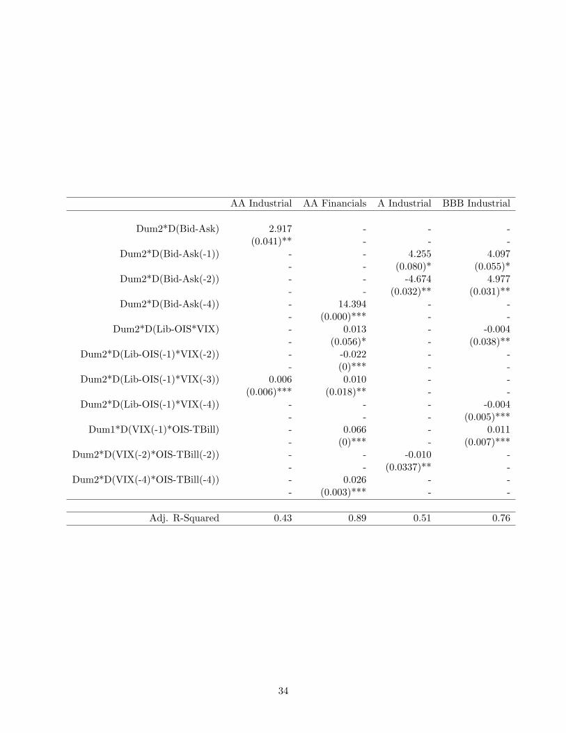
using the Error Correction Model Specification. Results are reported in table 9. For brevity of

exposition, in the table, I show only those variables that are significant21. Adjusted R-squared are

reported on the bottom of table.

INSERT TABLE 9 HERE

As for the long run regression, also in the short run regression, the relevant economic variables

tend to be significant, with expected signs, during the crisis period, moreover the signs of the

estimated parameters are generally consistent across the long and short run regressions. The error21Having 8 variable with 2 dummies and approximately 4 lags each, in the ECM estimation, the table would be

to big.

19

correction terms are significant with a negative sign, meaning that whenever bond spreads are

larger than CDS spreads they tend to revert to the long run equilibrium. This result is in line

with the results of paragraph 5. Further, as expected bond spread changes are positively related

to CDS changes to lagged bond spread changes, to Libor-OIS spread changes, to VIX changes and

to bid-ask spread changes. For AA financial and BBB industrials, for which the OIS-Tbill variable

has a negative impact in the long run regression, but also for AA industrials it has again a negative

impact in the short run regression.

Graphs 5 and 6, report the actual-fitted and residuals and show that the estimated model fits

the data quite well. The adjusted R-squared is on average 0.98 for the long run regression and

around 0.65 for the short run regression.

INSERT FIGURES 5 AND 6 HERE

5.3 Interpretation of the results

Since the beginning of the crisis, in July 2007, the perceived credit risk in the economy has

increased al well as the risk of default on interbank loans.

First, because of the general increase of default risk in the economy, CDS dealers (which are

financial institutions such as banks, insurance companies or hedge funds) are paying higher funding

rates. This effect is captured by the evolution of the Libor-OIS spread. A dramatic increase of cost

of financing has affected dealers’ CDS pricing as explained in section 3.2.22 The cost of financing

affects investors trading activities in a similar way. In order to exploit a negative basis an investor

must finance the purchase of the bond and buy protection. During the crisis the cost of financing,

if indeed financing is available, has increased substantially thus reducing or eliminating the return

to arbitrageurs. Also, because of the high market volatility, measured by mean of the VIX, margin

requirements (i.e. haircuts) for purchasing risky bonds (via repo transactions) have dramatically

increased (deterioration of funding liquidity); this has reduced the profitability and the possibility,22The lower bound on a dealers bid price for protection is provided by the net cost of financing the purchase

of the underlying cash bond. In normal conditions this cost approximates the bond spread and, in turn, the CDSspread. However, when the cost of financing increases the net cost falls and with it the CDS spread below whichit is worthwhile for the dealer to bid for protection while hedging in the cash market. Lowering the bid price forprotection also lowers the mid-price and, therefore, standard measures of the basis.

20

for investors, to implement basis trade, and explains the cross-sectional difference in the basis

across ratings, i.e. lower rated bonds and financials exhibit the most negative basis. It turns out

that funding liquidity constraints provide a source of commonality (Acharya and Pedersen 2005)

in explaining bond prices and returns, hence also the basis dynamics.

Second, liquidity has migrated from corporate bond market to the Treasury bond market,

driving risky bond yields larger. This ”flight to quality” effect is captured jointly by the evolution

of the OIS-Tbill spread and by the sharp increase of the VIX and CDS’s bid-asks spread.

Third, being CDS contracts an unfunded way of selling protection23, counterparty risk has

contributed driving bond spreads larger than CDS spreads. In fact, during the crisis protection

sellers (dealers which are mostly big banks) have higher default correlation to the assets being

protected. Default risk in the inter-bank lending market is captured, not only by the dynamics of

the CDS on banks, but also by the evolution of the Libor-OIS spread. This risk is priced into CDS

contracts of both financials and industrials driving their spreads lower irrespective of the actual

default intensity (discount).

Overall, results support the evidence that during the crisis the negative basis trade is largely

exposed to risk factors such as funding liquidity risk and counter-party risk, i.e. it is not risk-free.

The size of the basis is the return asked by investors on negative basis trades, hence it is a premium

due to exposure to systematic risk factors not an idiosyncratic arbitrage opportunity.

5.4 Robustness checks

The analysis reported above has been implemented also on single entities and results are

similar to those obtained on averages of credit spreads within rating groups. Investors carry out

basis trades on single entities, but common risk factors affects bases with similar underlying risks

in the a similar way. Also, results using daily data are similar to those obtained on weekly data.

Bond and CDS prices refers to mid-quotes not to real transactions. The focus of the paper is

on the systematic factors which drive discrepancies between CDS and bond spreads. Quotes are

well-behaved averages of transaction prices and are cleaned from the noise due to idiosyncratic

factors.

23While, bond being cash instruments, buying a corporate bond is a funded way of selling protection, hencecounterparty risk is not an issue. But the issue is the cost of financing the purchase of the bond itself.

21

Univariate analysis of the credit spreads time-series shows the presence of conditional hete-

orskedasticity (ARCH and GARCH Engle (1982)). For this reason I implement a cointegration test

that is robust to GARCH effects. I study the dynamic relationship between CDS and bond spreads

by the mean of a Vector Auto Regression, with the introduction of a tractable multivariate GARCH

formulation, such as the ”BEKK”, proposed by Engel and Kroner (1995). Results show that the

incorporation of the GARCH part allows to conclude more clearly that cointegration exists. The

presence of heteroskedasticity makes it more difficult to reject the null of no cointegration, but

since cointegration between CDS and bond spreads is found anyway, even without controlling for

GARCH effects, I do not implement this methodology in the analysis proposed in the paper.

The choice of the specification of the model in (section 5.2), has been for the univariate ECM,

which allows to easily account for the structural break by mean of period dummy variables. I run

the multivariate Johansen cointegration test on all the economic variables variables of equation (6)

jointly and I find that there is only one cointegration vector; this allows to use the univariate model.

The reason why I regress bond spreads on CDS is because CDS slightly dominate price discovery,

as shown in paragraph 5.1. and gives to the model a better fit. The analysis has also been carried

out estimating separately, for the pre-crisis and the crisis period with, the multivariate VECM and

gives results that are in line with those obtained using the univariate framework.

The structural break of August 2007 is modeled exogenously, because there is a general con-

sensus on the timing of the start of the 2007/08 financial crisis. One could think of modeling

the structural break by mean of a switching regime model, but in the sample period under study

(2006-2009), there is clear evidence of two states and there is no evidence of a switch between good

and bad states of the credit market conditions; it would be interesting to apply switching regime

models on credit spreads on longer samples which contain more crisis periods.

22

6 Conclusion

This paper documents that during the crisis, from July 2007 on, there are relevant price dis-

crepancies in the markets for credit risk: the basis is persistently negative, meaning that it would

be cheaper to take credit risk in the cash market, which has been quite infrequent in the past. In

principle, in such a situation, arbitrageurs could buy risky bonds hedge against default risk and

earn more that the risk free rate. Results show that during the crisis the negative basis trade is

largely exposed to risk factors such as funding liquidity risk and counter-party risk, i.e. it is not

risk-free. The size of the basis is the return asked by investors on negative basis trades, hence it is

a premium due to exposure to systematic risk factors not an idiosyncratic arbitrage opportunity.

Variables that capture the cost and risk factors of implementing the negative basis trade, such

as the Libor-OIS spread, the OIS-Tbill spread, the VIX and the bid-ask spread on CDS contracts,

are the main drivers of the basis dynamics in the period during the crisis. The Libor-OIS spread

captures all together (i) the funding cost and the funding liquidity risk faced by investors, (ii)

counter-party risk implicit into CDS spreads and (iii) corporate bond market liquidity deterioration

(Brunnermeier 2009). The OIS-Tbill spread is a measure of the ”Flight to quality” phenomenon.

The VIX is a measure of liquidity and risk premia in financial markets, but most importantly it

explains the bond value deterioration as a collateral. Finally, the bid-ask spread on CDS contracts

is a measure of general liquidity conditions in credit markets.

Results support the evidence that during stress times asset prices depart form frictionless ideals

due to funding liquidity risk faced by financial intermediaries and investors; hence, deviations from

parity do not imply presence of arbitrage opportunities. Funding liquidity constraints provide a

source of commonality (Acharya and Pedersen 2005) in explaining bond prices and returns, hence

also the basis dynamics.

23

References

Acharya, Viral V. Pedersen, Lasse Heje, 2005. Asset pricing with liquidity risk, Journal of FinancialEconomics, Elsevier, vol. 77(2)

Alexakis, Apergis, 1996. ARCH Effects and Cointegraiton: Is the foreign exchange market efficient?Journal of Banking and Finance.

Brenner R.J., Kroner K.F., 1995. Arbitrage, cointegration, and testing the unbiasedness hypothesisin financial markets. The Journal of Financial and Quantitative Analysis.

Brunnremeier, M. K. Deciphering the 2007-08. Liquidity and Credit Crunch’, 2009. Journal ofEconomic Perspectives.

Collin-Dufresene P, Goldstein S., Spencer Martin J., 2001. The determinants of credit spreadchanges. The Journal of Finance.

Garleanu N., Pedersen L, H., 2009. Margin based asset pricing and deviations from the law of oneprice. Working paper.

Duffie, Darrel,1999. Credit Swap valuation, Financial Analyst Journal 55.

Elton E.J., Gruber M.J., Agrawal D., Mann C., 2001. Explaining the rate spread on corporatebonds. The Journal of Finance.

Engle, Rober F. and Clive W.J. Granger 1987. Cointegration and error correction representation,estimation and testing. Econometrica 55.

Gonzalo, Jesus, and Clive W.J. Granger 1995. Estimation of common long-memory components incointegrated systems. Journal of Business and Economic Statistics 13.

Houweling, P and T. Vorst, 2003. Pricing default swaps: empirical evidence. Working paper.

Hull, John C., and Alan White, 2000a. Valuing credit default swaps: No counterparty default risk.Journal of derivatives 8.

Jan De Wit, 2006. Exploring the CDS-bond basis. National Bank of Belgium, Working paper n.104

Longstaff, Mithal, Neis, 2005. Corporate yield spreads: default risk or liquidity? New evidencefrom the credit default swap market. Journal of Finance 5.

Lucy F. Ackert, M.D. Racine,1999. Stochastic trends and Cointegration in the market for equities.Journal of Economics and business. 51.

Norden Weber, 2004. The co-movement of CDS, bond and stock markets: an empirical anlaysis.CFS working paper.

Roberto Blanco, Simon Brennan Ian Marsh, 2005. An empirical analysis of the dynamic relationbetween investment grade bonds and Credit Default Swaps, Journal of Finance 5.

Robin J. Brenner, Kenneth F. Kroner, 1995. Arbitrage, cointegration, and testing the unbiasednesshypothesis in financial markets. The Journal of Financial and Quantitative Analysis. Vol 30.

24

Tae-Hwy Lee, Yiuman Tse, 1996 Cointegration test with conditional heteroskedasticity. Journal ofEconometrics.

Zhu, 2004. An empirical comparison of credit spreads between the bond market and the creditdefault swp market. BIS working paper.

25

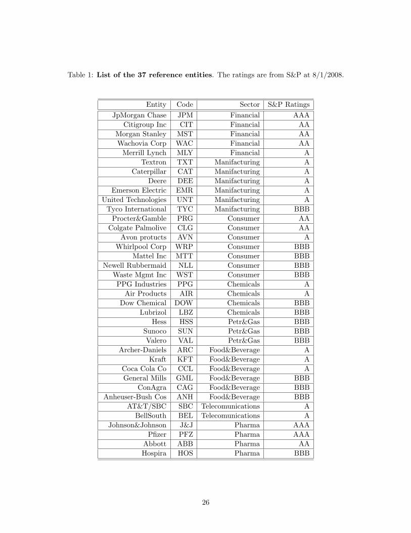
Table 1: List of the 37 reference entities. The ratings are from S&P at 8/1/2008.

Entity Code Sector S&P RatingsJpMorgan Chase JPM Financial AAA

Citigroup Inc CIT Financial AAMorgan Stanley MST Financial AAWachovia Corp WAC Financial AA

Merrill Lynch MLY Financial ATextron TXT Manifacturing A

Caterpillar CAT Manifacturing ADeere DEE Manifacturing A

Emerson Electric EMR Manifacturing AUnited Technologies UNT Manifacturing A

Tyco International TYC Manifacturing BBBProcter&Gamble PRG Consumer AA

Colgate Palmolive CLG Consumer AAAvon protucts AVN Consumer A

Whirlpool Corp WRP Consumer BBBMattel Inc MTT Consumer BBB

Newell Rubbermaid NLL Consumer BBBWaste Mgmt Inc WST Consumer BBBPPG Industries PPG Chemicals A

Air Products AIR Chemicals ADow Chemical DOW Chemicals BBB

Lubrizol LBZ Chemicals BBBHess HSS Petr&Gas BBB

Sunoco SUN Petr&Gas BBBValero VAL Petr&Gas BBB

Archer-Daniels ARC Food&Beverage AKraft KFT Food&Beverage A

Coca Cola Co CCL Food&Beverage AGeneral Mills GML Food&Beverage BBB

ConAgra CAG Food&Beverage BBBAnheuser-Bush Cos ANH Food&Beverage BBB

AT&T/SBC SBC Telecomunications ABellSouth BEL Telecomunications A

Johnson&Johnson J&J Pharma AAAPfizer PFZ Pharma AAA

Abbott ABB Pharma AAHospira HOS Pharma BBB

26

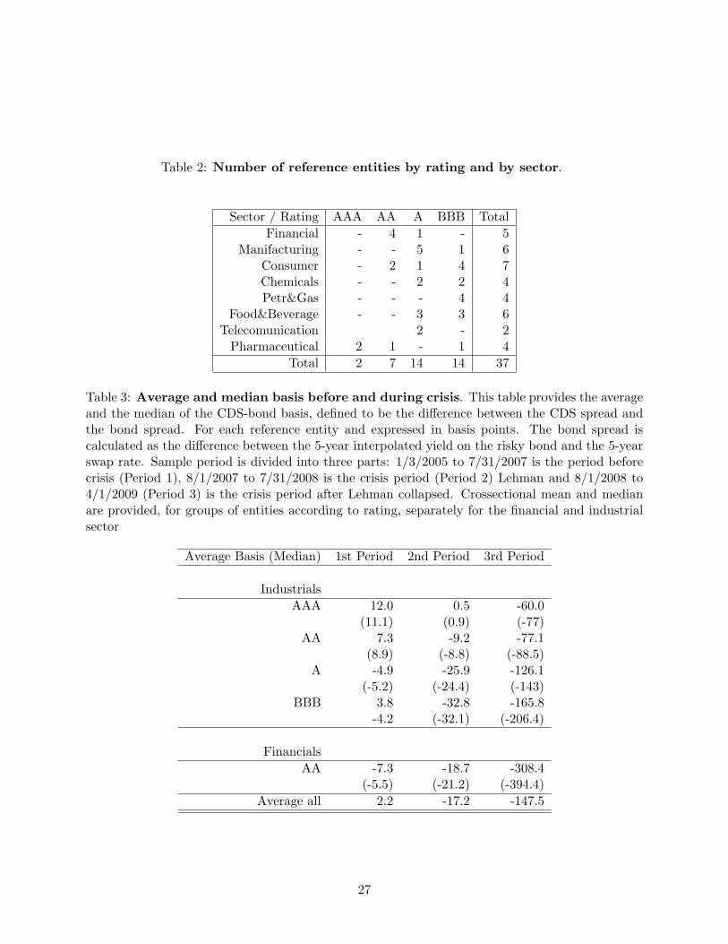
Table 2: Number of reference entities by rating and by sector.

Sector / Rating AAA AA A BBB TotalFinancial - 4 1 - 5

Manifacturing - - 5 1 6Consumer - 2 1 4 7Chemicals - - 2 2 4Petr&Gas - - - 4 4

Food&Beverage - - 3 3 6Telecomunication 2 - 2

Pharmaceutical 2 1 - 1 4Total 2 7 14 14 37

Table 3: Average and median basis before and during crisis. This table provides the averageand the median of the CDS-bond basis, defined to be the difference between the CDS spread andthe bond spread. For each reference entity and expressed in basis points. The bond spread iscalculated as the difference between the 5-year interpolated yield on the risky bond and the 5-yearswap rate. Sample period is divided into three parts: 1/3/2005 to 7/31/2007 is the period beforecrisis (Period 1), 8/1/2007 to 7/31/2008 is the crisis period (Period 2) Lehman and 8/1/2008 to4/1/2009 (Period 3) is the crisis period after Lehman collapsed. Crossectional mean and medianare provided, for groups of entities according to rating, separately for the financial and industrialsector

Average Basis (Median) 1st Period 2nd Period 3rd Period

IndustrialsAAA 12.0 0.5 -60.0

(11.1) (0.9) (-77)AA 7.3 -9.2 -77.1

(8.9) (-8.8) (-88.5)A -4.9 -25.9 -126.1

(-5.2) (-24.4) (-143)BBB 3.8 -32.8 -165.8

-4.2 (-32.1) (-206.4)

FinancialsAA -7.3 -18.7 -308.4

(-5.5) (-21.2) (-394.4)Average all 2.2 -17.2 -147.5

27

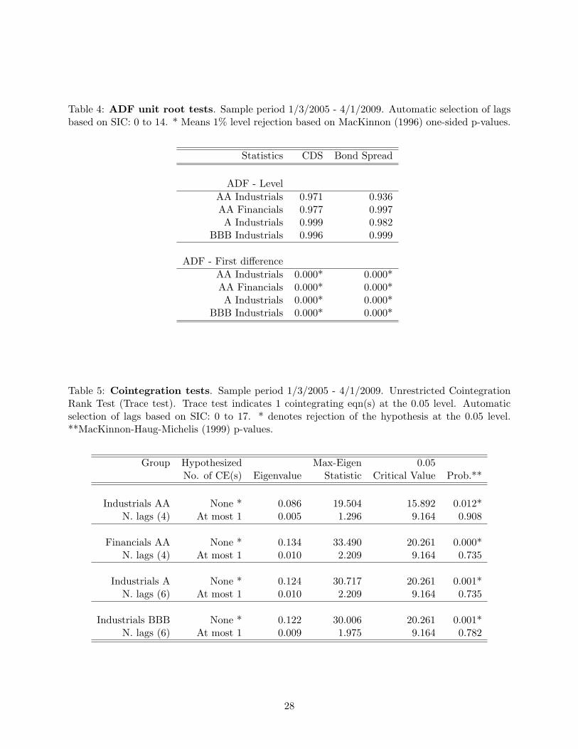
Table 4: ADF unit root tests. Sample period 1/3/2005 - 4/1/2009. Automatic selection of lagsbased on SIC: 0 to 14. * Means 1% level rejection based on MacKinnon (1996) one-sided p-values.

Statistics CDS Bond Spread

ADF - LevelAA Industrials 0.971 0.936AA Financials 0.977 0.997A Industrials 0.999 0.982

BBB Industrials 0.996 0.999

ADF - First differenceAA Industrials 0.000* 0.000*AA Financials 0.000* 0.000*A Industrials 0.000* 0.000*

BBB Industrials 0.000* 0.000*

Table 5: Cointegration tests. Sample period 1/3/2005 - 4/1/2009. Unrestricted CointegrationRank Test (Trace test). Trace test indicates 1 cointegrating eqn(s) at the 0.05 level. Automaticselection of lags based on SIC: 0 to 17. * denotes rejection of the hypothesis at the 0.05 level.**MacKinnon-Haug-Michelis (1999) p-values.

Group Hypothesized Max-Eigen 0.05No. of CE(s) Eigenvalue Statistic Critical Value Prob.**

Industrials AA None * 0.086 19.504 15.892 0.012*N. lags (4) At most 1 0.005 1.296 9.164 0.908

Financials AA None * 0.134 33.490 20.261 0.000*N. lags (4) At most 1 0.010 2.209 9.164 0.735

Industrials A None * 0.124 30.717 20.261 0.001*N. lags (6) At most 1 0.010 2.209 9.164 0.735

Industrials BBB None * 0.122 30.006 20.261 0.001*N. lags (6) At most 1 0.009 1.975 9.164 0.782

28

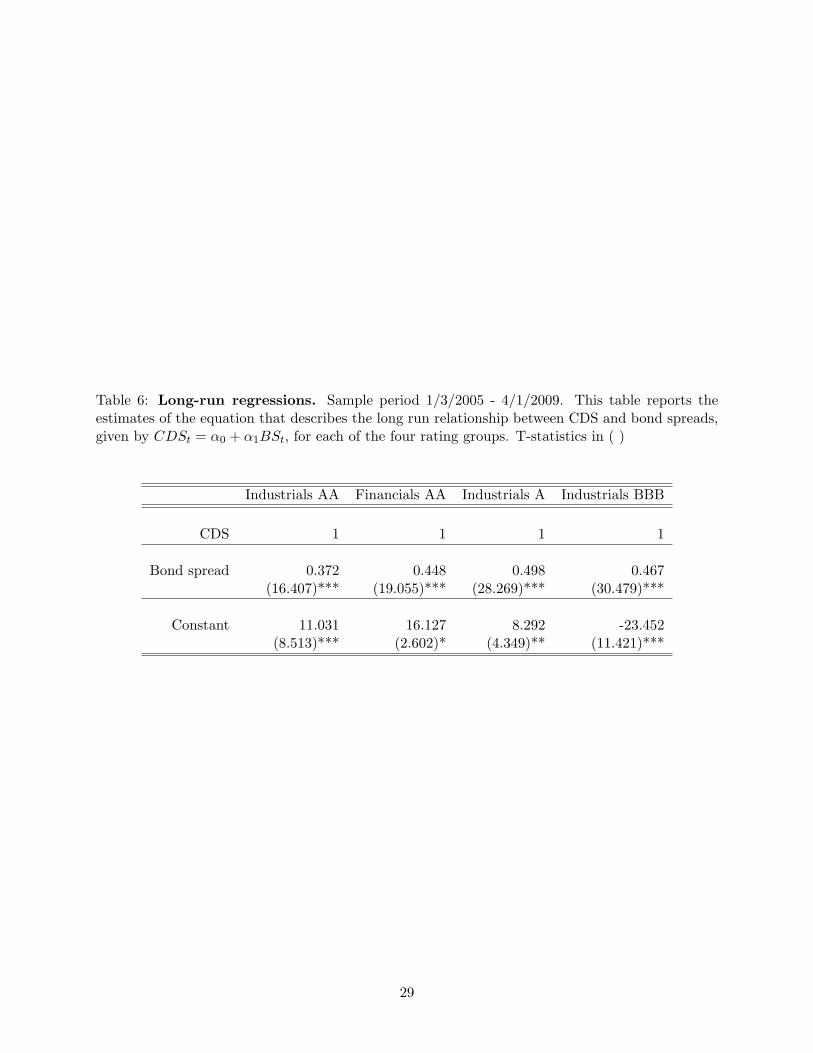
Table 6: Long-run regressions. Sample period 1/3/2005 - 4/1/2009. This table reports theestimates of the equation that describes the long run relationship between CDS and bond spreads,given by CDSt = α0 + α1BSt, for each of the four rating groups. T-statistics in ( )

Industrials AA Financials AA Industrials A Industrials BBB

CDS 1 1 1 1

Bond spread 0.372 0.448 0.498 0.467(16.407)*** (19.055)*** (28.269)*** (30.479)***

Constant 11.031 16.127 8.292 -23.452(8.513)*** (2.602)* (4.349)** (11.421)***

29

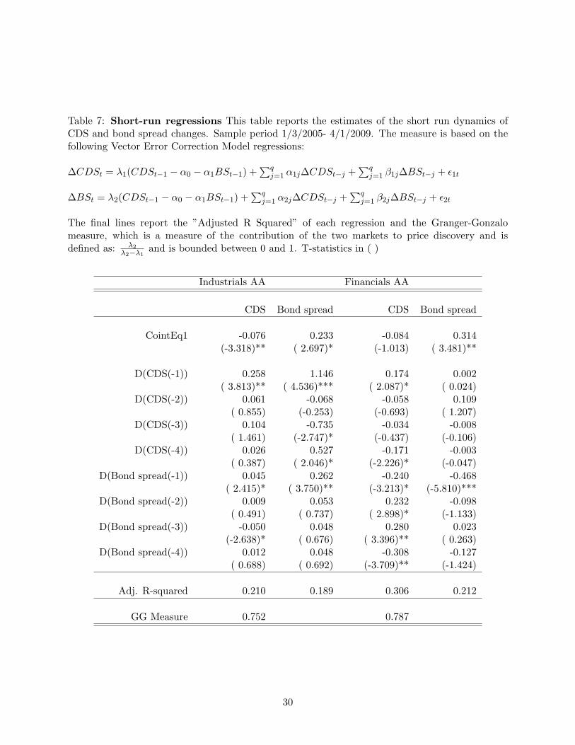
Table 7: Short-run regressions This table reports the estimates of the short run dynamics ofCDS and bond spread changes. Sample period 1/3/2005- 4/1/2009. The measure is based on thefollowing Vector Error Correction Model regressions:

∆CDSt = λ1(CDSt−1 − α0 − α1BSt−1) +∑q

j=1 α1j∆CDSt−j +∑q

j=1 β1j∆BSt−j + ε1t

∆BSt = λ2(CDSt−1 − α0 − α1BSt−1) +∑q

j=1 α2j∆CDSt−j +∑q

j=1 β2j∆BSt−j + ε2t

The final lines report the ”Adjusted R Squared” of each regression and the Granger-Gonzalomeasure, which is a measure of the contribution of the two markets to price discovery and isdefined as: λ2

λ2−λ1and is bounded between 0 and 1. T-statistics in ( )

Industrials AA Financials AA

CDS Bond spread CDS Bond spread

CointEq1 -0.076 0.233 -0.084 0.314(-3.318)** ( 2.697)* (-1.013) ( 3.481)**

D(CDS(-1)) 0.258 1.146 0.174 0.002( 3.813)** ( 4.536)*** ( 2.087)* ( 0.024)

D(CDS(-2)) 0.061 -0.068 -0.058 0.109( 0.855) (-0.253) (-0.693) ( 1.207)

D(CDS(-3)) 0.104 -0.735 -0.034 -0.008( 1.461) (-2.747)* (-0.437) (-0.106)

D(CDS(-4)) 0.026 0.527 -0.171 -0.003( 0.387) ( 2.046)* (-2.226)* (-0.047)

D(Bond spread(-1)) 0.045 0.262 -0.240 -0.468( 2.415)* ( 3.750)** (-3.213)* (-5.810)***

D(Bond spread(-2)) 0.009 0.053 0.232 -0.098( 0.491) ( 0.737) ( 2.898)* (-1.133)

D(Bond spread(-3)) -0.050 0.048 0.280 0.023(-2.638)* ( 0.676) ( 3.396)** ( 0.263)

D(Bond spread(-4)) 0.012 0.048 -0.308 -0.127( 0.688) ( 0.692) (-3.709)** (-1.424)

Adj. R-squared 0.210 0.189 0.306 0.212

GG Measure 0.752 0.787

30

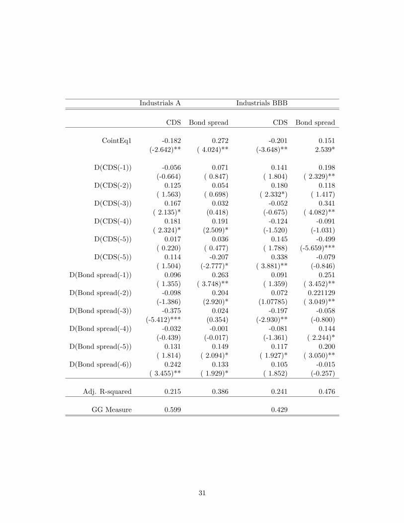
Industrials A Industrials BBB

CDS Bond spread CDS Bond spread

CointEq1 -0.182 0.272 -0.201 0.151(-2.642)** ( 4.024)** (-3.648)** 2.539*

D(CDS(-1)) -0.056 0.071 0.141 0.198(-0.664) ( 0.847) ( 1.804) ( 2.329)**

D(CDS(-2)) 0.125 0.054 0.180 0.118( 1.563) ( 0.698) ( 2.332*) ( 1.417)

D(CDS(-3)) 0.167 0.032 -0.052 0.341( 2.135)* (0.418) (-0.675) ( 4.082)**

D(CDS(-4)) 0.181 0.191 -0.124 -0.091( 2.324)* (2.509)* (-1.520) (-1.031)

D(CDS(-5)) 0.017 0.036 0.145 -0.499( 0.220) ( 0.477) ( 1.788) (-5.659)***

D(CDS(-5)) 0.114 -0.207 0.338 -0.079( 1.504) (-2.777)* ( 3.881)** (-0.846)

D(Bond spread(-1)) 0.096 0.263 0.091 0.251( 1.355) ( 3.748)** ( 1.359) ( 3.452)**

D(Bond spread(-2)) -0.098 0.204 0.072 0.221129(-1.386) (2.920)* (1.07785) ( 3.049)**

D(Bond spread(-3)) -0.375 0.024 -0.197 -0.058(-5.412)*** (0.354) (-2.930)** (-0.800)

D(Bond spread(-4)) -0.032 -0.001 -0.081 0.144(-0.439) (-0.017) (-1.361) ( 2.244)*

D(Bond spread(-5)) 0.131 0.149 0.117 0.200( 1.814) ( 2.094)* ( 1.927)* ( 3.050)**

D(Bond spread(-6)) 0.242 0.133 0.105 -0.015( 3.455)** ( 1.929)* ( 1.852) (-0.257)

Adj. R-squared 0.215 0.386 0.241 0.476

GG Measure 0.599 0.429

31

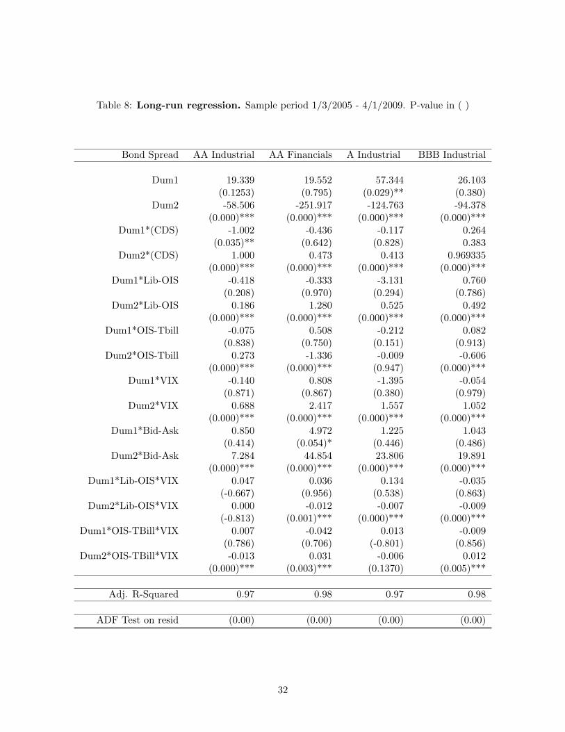
Table 8: Long-run regression. Sample period 1/3/2005 - 4/1/2009. P-value in ( )

Bond Spread AA Industrial AA Financials A Industrial BBB Industrial

Dum1 19.339 19.552 57.344 26.103(0.1253) (0.795) (0.029)** (0.380)

Dum2 -58.506 -251.917 -124.763 -94.378(0.000)*** (0.000)*** (0.000)*** (0.000)***

Dum1*(CDS) -1.002 -0.436 -0.117 0.264(0.035)** (0.642) (0.828) 0.383

Dum2*(CDS) 1.000 0.473 0.413 0.969335(0.000)*** (0.000)*** (0.000)*** (0.000)***

Dum1*Lib-OIS -0.418 -0.333 -3.131 0.760(0.208) (0.970) (0.294) (0.786)

Dum2*Lib-OIS 0.186 1.280 0.525 0.492(0.000)*** (0.000)*** (0.000)*** (0.000)***

Dum1*OIS-Tbill -0.075 0.508 -0.212 0.082(0.838) (0.750) (0.151) (0.913)

Dum2*OIS-Tbill 0.273 -1.336 -0.009 -0.606(0.000)*** (0.000)*** (0.947) (0.000)***

Dum1*VIX -0.140 0.808 -1.395 -0.054(0.871) (0.867) (0.380) (0.979)

Dum2*VIX 0.688 2.417 1.557 1.052(0.000)*** (0.000)*** (0.000)*** (0.000)***

Dum1*Bid-Ask 0.850 4.972 1.225 1.043(0.414) (0.054)* (0.446) (0.486)

Dum2*Bid-Ask 7.284 44.854 23.806 19.891(0.000)*** (0.000)*** (0.000)*** (0.000)***

Dum1*Lib-OIS*VIX 0.047 0.036 0.134 -0.035(-0.667) (0.956) (0.538) (0.863)

Dum2*Lib-OIS*VIX 0.000 -0.012 -0.007 -0.009(-0.813) (0.001)*** (0.000)*** (0.000)***

Dum1*OIS-TBill*VIX 0.007 -0.042 0.013 -0.009(0.786) (0.706) (-0.801) (0.856)

Dum2*OIS-TBill*VIX -0.013 0.031 -0.006 0.012(0.000)*** (0.003)*** (0.1370) (0.005)***

Adj. R-Squared 0.97 0.98 0.97 0.98

ADF Test on resid (0.00) (0.00) (0.00) (0.00)

32

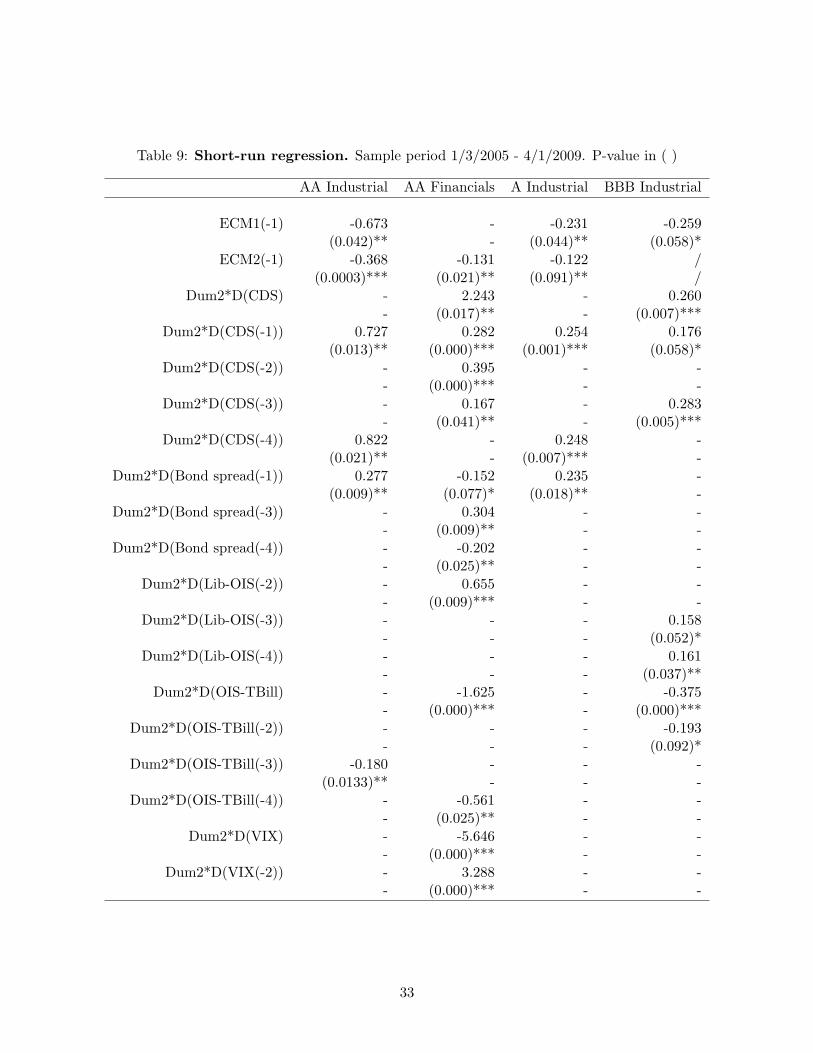
Table 9: Short-run regression. Sample period 1/3/2005 - 4/1/2009. P-value in ( )

AA Industrial AA Financials A Industrial BBB Industrial

ECM1(-1) -0.673 - -0.231 -0.259(0.042)** - (0.044)** (0.058)*

ECM2(-1) -0.368 -0.131 -0.122 /(0.0003)*** (0.021)** (0.091)** /

Dum2*D(CDS) - 2.243 - 0.260- (0.017)** - (0.007)***

Dum2*D(CDS(-1)) 0.727 0.282 0.254 0.176(0.013)** (0.000)*** (0.001)*** (0.058)*

Dum2*D(CDS(-2)) - 0.395 - -- (0.000)*** - -

Dum2*D(CDS(-3)) - 0.167 - 0.283- (0.041)** - (0.005)***

Dum2*D(CDS(-4)) 0.822 - 0.248 -(0.021)** - (0.007)*** -

Dum2*D(Bond spread(-1)) 0.277 -0.152 0.235 -(0.009)** (0.077)* (0.018)** -

Dum2*D(Bond spread(-3)) - 0.304 - -- (0.009)** - -

Dum2*D(Bond spread(-4)) - -0.202 - -- (0.025)** - -

Dum2*D(Lib-OIS(-2)) - 0.655 - -- (0.009)*** - -

Dum2*D(Lib-OIS(-3)) - - - 0.158- - - (0.052)*

Dum2*D(Lib-OIS(-4)) - - - 0.161- - - (0.037)**

Dum2*D(OIS-TBill) - -1.625 - -0.375- (0.000)*** - (0.000)***

Dum2*D(OIS-TBill(-2)) - - - -0.193- - - (0.092)*

Dum2*D(OIS-TBill(-3)) -0.180 - - -(0.0133)** - - -

Dum2*D(OIS-TBill(-4)) - -0.561 - -- (0.025)** - -

Dum2*D(VIX) - -5.646 - -- (0.000)*** - -

Dum2*D(VIX(-2)) - 3.288 - -- (0.000)*** - -

33

AA Industrial AA Financials A Industrial BBB Industrial

Dum2*D(Bid-Ask) 2.917 - - -(0.041)** - - -

Dum2*D(Bid-Ask(-1)) - - 4.255 4.097- - (0.080)* (0.055)*

Dum2*D(Bid-Ask(-2)) - - -4.674 4.977- - (0.032)** (0.031)**

Dum2*D(Bid-Ask(-4)) - 14.394 - -- (0.000)*** - -

Dum2*D(Lib-OIS*VIX) - 0.013 - -0.004- (0.056)* - (0.038)**

Dum2*D(Lib-OIS(-1)*VIX(-2)) - -0.022 - -- (0)*** - -

Dum2*D(Lib-OIS(-1)*VIX(-3)) 0.006 0.010 - -(0.006)*** (0.018)** - -

Dum2*D(Lib-OIS(-1)*VIX(-4)) - - - -0.004- - - (0.005)***

Dum1*D(VIX(-1)*OIS-TBill) - 0.066 - 0.011- (0)*** - (0.007)***

Dum2*D(VIX(-2)*OIS-TBill(-2)) - - -0.010 -- - (0.0337)** -

Dum2*D(VIX(-4)*OIS-TBill(-4)) - 0.026 - -- (0.003)*** - -

Adj. R-Squared 0.43 0.89 0.51 0.76

34

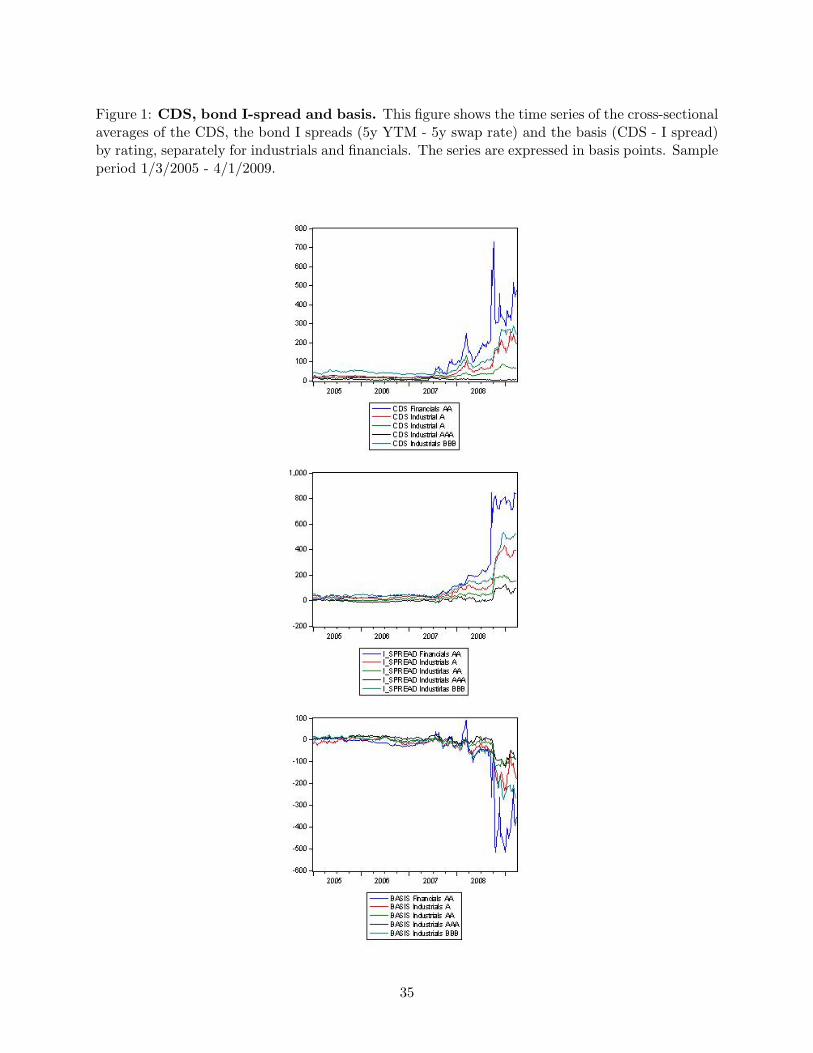
Figure 1: CDS, bond I-spread and basis. This figure shows the time series of the cross-sectionalaverages of the CDS, the bond I spreads (5y YTM - 5y swap rate) and the basis (CDS - I spread)by rating, separately for industrials and financials. The series are expressed in basis points. Sampleperiod 1/3/2005 - 4/1/2009.

35

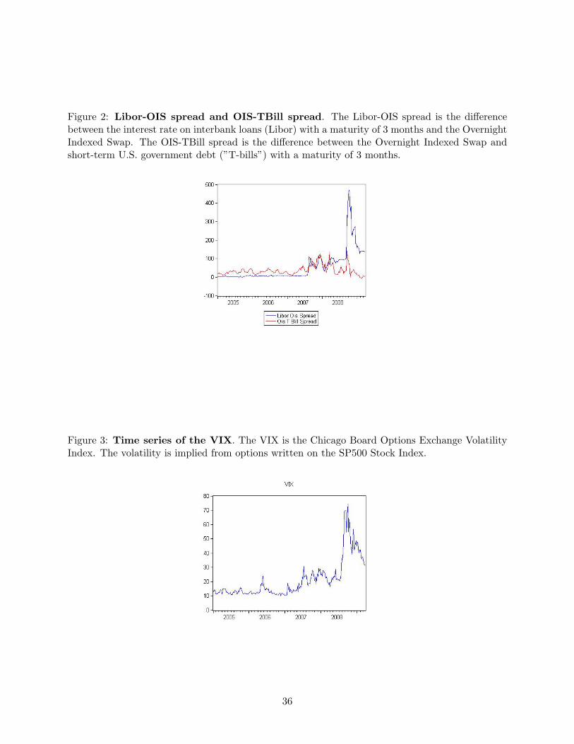
Figure 2: Libor-OIS spread and OIS-TBill spread. The Libor-OIS spread is the differencebetween the interest rate on interbank loans (Libor) with a maturity of 3 months and the OvernightIndexed Swap. The OIS-TBill spread is the difference between the Overnight Indexed Swap andshort-term U.S. government debt (”T-bills”) with a maturity of 3 months.

Figure 3: Time series of the VIX. The VIX is the Chicago Board Options Exchange VolatilityIndex. The volatility is implied from options written on the SP500 Stock Index.

36

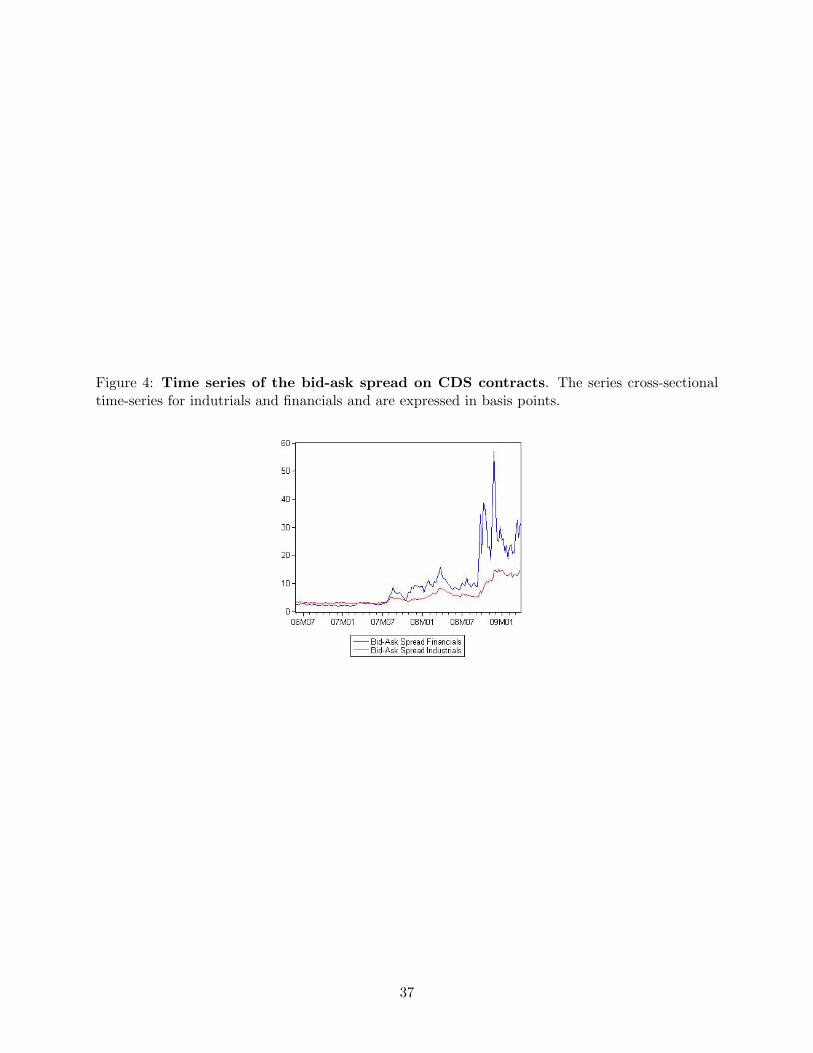
Figure 4: Time series of the bid-ask spread on CDS contracts. The series cross-sectionaltime-series for indutrials and financials and are expressed in basis points.

37

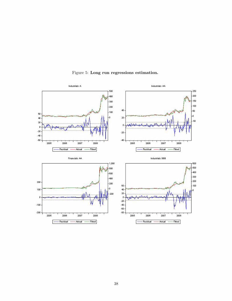
Figure 5: Long run regressions estimation.

38

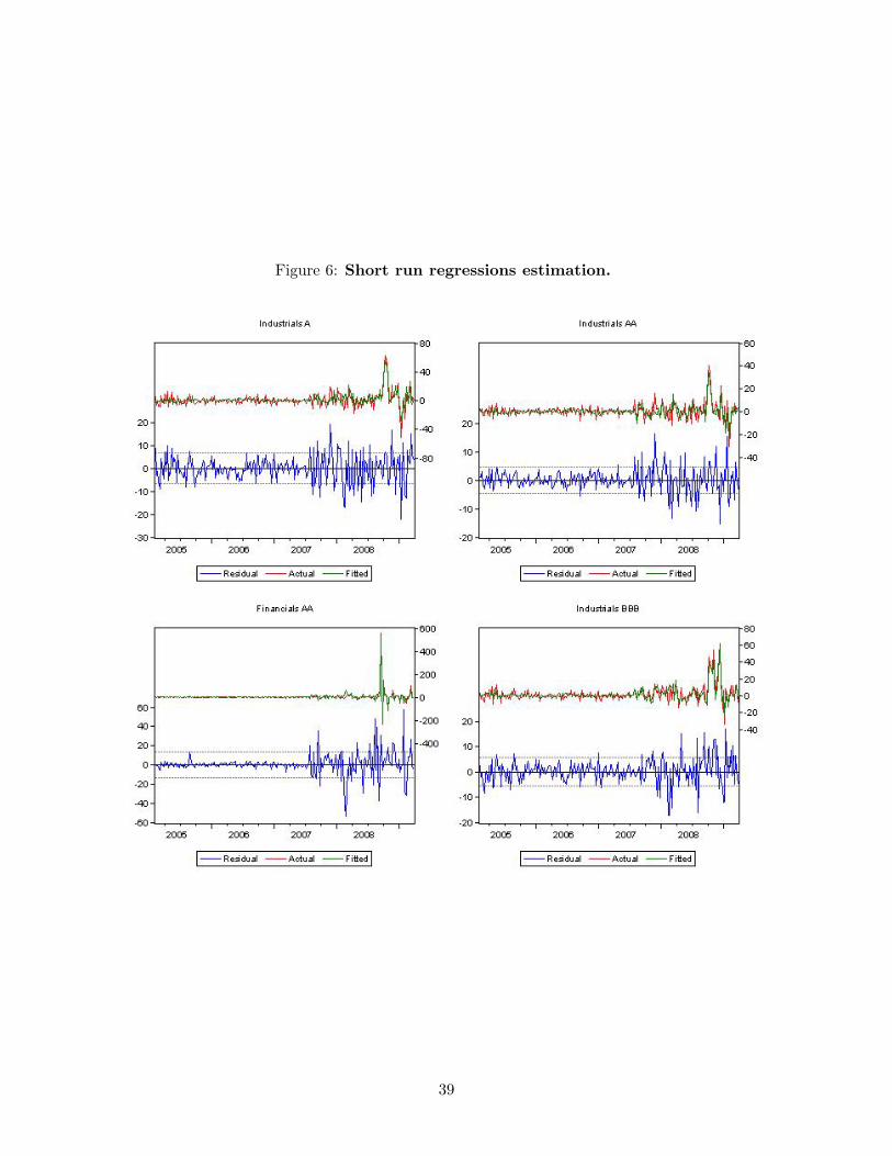
Figure 6: Short run regressions estimation.

39