the persistent cold-air pool study

THE PERSISTENT COLD-AIR POOL STUDY

BY NEIL P. LAREAU, ERIK CROSMAN, C. DAVID WHITEMAN, JOHN D. HOREL, SEBASTIAN W. HOCH, WILLIAM O. J. BROWN, AND THOMAS W. HORST

Utah's Salt Lake valley was the setting for a wintertime study of multiday cold-air pools that affect air quality in urban basins.

A cold-air pool (CAP), defined as a topographic depression filled with cold air, occurs when atmospheric processes favor cooling of the air near the surface, warming of the air aloft, or both. The resulting stable stratification prevents the

air within the basin from mixing with the atmosphere aloft while the surrounding topography prevents lateral displacement and favors air stagnation. CAPs are common in mountain valleys during periods of light winds, high atmospheric pressure, and low insolation (Daly et al. 2009).

CAPs may be classified as diurnal, forming during the night and decaying the following day, or persistent, lasting multiple days (Whiteman et al. 2001). Diurnal CAPs are generally dominated by radiational cooling and are often associated with a surface-based temperature inversion. They accumulate in depth throughout the night only to be destroyed the next day by the growth of the convective boundary layer (CBL; Kondo et al. 1989; Whiteman et al. 2008). These short-lived CAPs have been studied in numerous field campaigns (Neff and King 1989; Clements et al. 2003; Doran et al. 2002; Whiteman et al. 2008; Price et al. 2011).

Persistent CAPs are considerably more complex and arise because of a multitude of atmospheric processes. At large scales, differential temperature advection and sub-sidence modulate CAP strength and duration, while mesoscale flows and radiative, turbulent, and cloud processes likewise affect their evolution (Wolyn and McKee 1989; Whiteman et al. 1999, 2001; Zhong et al. 2001; Reeves and Stensrud 2009; Gillies et al. 2010). When these long-lived CAPs occur within urbanized basins,

Looking west across the Salt Lake valley during a fog and pollution filled cold-air pool on 14 Jan. 2011 (Photo courtesy of Sebastian Hoch).

AFFILIATIONS: LAREAU, CROSMAN, WHITEMAN, HOREL, AND HOCH— Department of Atmospheric Sciences, University of Utah, Salt Lake City, Utah; BROWN AND HORST—National Center for Atmospheric Research, Boulder, ColoradoCORRESPONDING AUTHOR: Neil P. Lareau, 135 South 1460 East, Room 819, Salt Lake City, UT 84112-0110E-mail: [email protected]

The abstract for this article can be found in this issue, following the table of contents.DOI:10.1175/BAMS-D-11-00255.1

In final form 2 April 2012©2013 American Meteorological Society

the emissions from vehicles, home heating, and indus-trial sources accumulate within the stagnant air and can lead to hazardous air quality (Reddy et al. 1995; Pataki et al. 2005, 2006; Malek et al. 2006; Silcox et al. 2012). Dense fog, low clouds, and light precipitation may also occur and can adversely impact air and ground transportation.

Despite their societal impacts, persistent CAPs are not thoroughly understood and the mechanisms governing CAP evolution are not well documented because of the limited observational resources avail-able to previous researchers (e.g., Wolyn and McKee 1989; Reeves and Stensrud 2009; Gillies et al. 2010). Moreover, persistent CAPs are generally inadequately resolved in forecast models, and even small model errors can have large impacts on temperature and air quality forecasts (Reeves et al. 2011). One source of forecast error is operational turbulent mixing and diffusion parameterizations, which perform poorly in strongly stable environments and complex terrain (Zängl 2002; Fernando and Weil 2010; Baklanov et al. 2011; Baker et al. 2011; Reeves et al. 2011).

The Persistent Cold-Air Pool Study (PCAPS) addressed the need for modern observations capable of resolving the hierarchy of scales affecting persistent CAPs. PCAPS is part of a broader 3-yr investigation supported by the National Science Foundation for which the goals are as follows: to understand the processes governing the life cycle of persistent CAPs, to determine the consequence of these processes on air pollution, and to improve the fidelity of forecasts of persistent CAPs. The remainder of this paper provides an overview of the PCAPS experiment design, instrumentation, and initial research findings.

THE PERSISTENT COLD -AIR POOL STUDY. The Salt Lake valley. PCAPS was conducted in the Salt Lake valley (SLV) of northern Utah (Fig. 1).

The SLV (~1,300 MSL) is a small portion (~30 km2) of a larger basin encompassing much of northwest Utah including the Great Salt Lake (GSL). It is home to ~1 million residents. The valley is confined by the Wasatch (~3,000 MSL) and Oquirrh (~2,500 MSL) Mountains to its east and west, respectively, and separated from the neighboring Utah valley to its south by the lower Traverse Mountains. The Jordan Narrows gap allows exchange of air between the two valleys (Chen et al. 2004; Pinto et al. 2006). A series of steep east–west-trending canyons is incised into the Wasatch while the Oquirrhs feature comparatively broad slopes.

CAPs are common in the SLV during winter and often accompanied with unhealthy air qual-ity and occasional episodes of dense fog. The 24-h mean concentration of fine particulate aerosol with diameters less that 2.5 μm (PM2.5) often exceeds the National Ambient Air Quality Standard (NAAQS) of 35 μg m−3 during persistent CAP episodes (U.S. EPA 2011; Silcox et al. 2012). High levels of carbon dioxide, carbon monoxide, and ozone may also occur (Pataki et al. 2005, 2006). Emergency room visits with a pri-mary diagnosis of asthma are suggested to be 42% higher during the late stages of prolonged CAP events compared to non-CAP days (Utah Asthma Program 2010). Public awareness of the adverse health effects of inversions (the colloquial term for CAPs) is increasing and a number of local groups are advocating steps to reduce them.

Experiment design. University of Utah graduate students played a prominent role in the experimen-tal design and implementation of the PCAPS field campaign. In collaboration with the project’s principal investigators, they devised a two-tiered observational strategy for documenting the life cycle of persistent CAPs. First, continuously operating meteorological instruments were distributed throughout the Salt Lake valley to provide data during the entire field campaign. Second, intensive observation periods (IOPs) were declared whenever a CAP was expected to form and persist for more than one day. During each IOP, additional resources were deployed to target the specific physical processes expected to impact CAP evolution. Real-time observations from PCAPS instrumentation were subsequently used to fine-tune IOP operations as each event unfolded.

Instrumentation. In this section, we detail the observing platforms used during PCAPS. Observing sites are shown in Fig. 1, and photographs of many of the instruments are included in Fig. 2.

2 JANUARY 2013|

R E M O T E S E N S O R S . Two N a t i o n a l C e n t e r f o r Atmospheric Research (NCAR) radar wind pro-filers, a scanning pulsed Doppler lidar, and a mini-sodar (Figs. 2d–f) provided continuous observations of winds above the SLV during PCAPS. The radar wind profilers (915 and 449 MHz), located in the valley center, character-ized the wind shear within and above (~200–3,000 m AGL) each CAP as well as the occasional penetration of strong winds into the valley atmosphere. Changes in wind occurring closer to the ground (20–200 m AGL) were determined with the minisodar that was situated near the GSL to observe land and lake breezes. The lidar provided additional observations of winds aloft along the west-ern edge of the SLV.

The vertical tempera-ture structure within the SLV was observed with a Radio Acoustic Sounding System (RASS; Fig. 2e), which operated in concert with the 915-MHz radar. Data from the RASS pro-vide high temporal sampling during periods of rapid transition. Additional measurements of temperatures aloft were collected with a microwave radiometer.

A laser ceilometer, located at the NCAR Integrated Sounding System (ISS) site, ~0.5 km south of the profilers, was used to measure aerosol and hydrome-teor backscatter (Fig. 2g). These data are particularly useful in visualizing boundary layer structure and provide an objective indication for the presence of low and midlevel clouds.

SURFACE METEOROLOGICAL STATIONS. Monitoring the complete surface energy balance at seven locations distributed throughout the SLV (Fig. 1) was of funda-mental importance during PCAPS. These sites were chosen to span the geographical extent of the valley and to represent varying land use, ranging from urban to agricultural. Each location housed an NCAR Integrated Surface Flux Station (ISFS) equipped with a three-

dimensional (3D) sonic anemometer, fast response temperature and humidity sensors, solar and terrestrial radiometers, and soil temperature probes (Fig. 2a).

Five automated weather stations (Fig. 2b) were installed at the south end of the SLV along a vertical transect of the Traverse Mountains (Fig. 1) to moni-tor variations in wind, temperature, and humidity during CAPs. These sites are also useful in diagnosing a cross-barrier exchange between the Utah and Salt Lake valleys (Chen et al. 2004; Pinto et al. 2006).

Additional vertical profiles of temperature and humidity were established with Hobo dataloggers distributed at 50-m elevation increments along three transects: one ascending a prominent ridge on the west slope of the Wasatch Mountains and two along the east slopes of the Oquirrh Mountains. Recording measurements every 5 min, these datalog-gers provide temperature pseudosoundings capable of documenting rapid changes in the vertical ther-modynamic structure.

The PCAPS field campaign also benefitted from more than 100 preexisting surface meteorological

FIG. 1. Relief map showing location of PCAPS field campaign instrumentation. Green circles denote the location of Hobo dataloggers on the valley sidewalls. Purple circles and white numbers denote the seven NCAR ISFSs. Blue circles indicate the two NCAR ISS facilities, and a red plus symbol denotes the sodar site. Yellow circles indicate University of Utah automated weather stations, while preexisting MesoWest surface stations are indicated with black plus symbols. The Salt Lake International Airport is denoted as a black dot. The locations of special radiosonde launches during specific IOPs are indicated by red triangles, while a blue plus shows the location of the lidar. The Hawthorne elementary school DAQ site is shown as a pink triangle. Mobile weather station transects, glider flight paths, and additional air quality monitoring locations are not shown on the map.

3JANUARY 2013AMERICAN METEOROLOGICAL SOCIETY |

stations distributed in and around the SLV. These data, available through MesoWest (Horel et al. 2002), provide observations of the spatial heterogeneity within the CAPs.

An air quality observation network, operated by the Utah Division of Air Quality (DAQ), provided hourly and 24-h mean measurements of criterion pollutants, including concentrations of PM2.5. This network was supplemented by a line of PM2.5 samplers that ran up a sloping neighborhood at the north end of the SLV (Silcox et al. 2012).

IOP OBSERVATIONS. Radiosondes launched from the NCAR ISS site provided the principal observations of CAP thermodynamic structure during each IOP. Over 115 Vaisala radiosondes were launched throughout the project, augmenting the 138 regu-larly scheduled twice-daily National Weather Service (NWS) soundings deployed at the nearby Salt Lake International Airport (Fig. 1). The temporal interval

of the ISS soundings ranged from once every 3 h during periods of rapid transition to once a day for routine monitoring of CAPs.

Three additional mobile radiosonde systems (Graw) were used at sites throughout the SLV to provide contemporaneous thermodynamic profiles during targeted observations of lake-breeze fronts, periods of differential sidewall heating, canyon drain-age flows, and partial “mix out” of the CAP during strong winds. In total 57, Graw radiosondes were deployed, significantly enhancing sampling of the spatial variability in CAP vertical structure.

A powered paraglider (Fig. 2j) equipped with tem-perature, humidity, and pressure sensors was used on 5 IOP days to perform horizontal boundary layer transects and repeated vertical profiles. Some of the unique observations collected by the paraglider are described in the sidebar.

In addition to enhanced upper-air observa-tions, surface meteorological measurements were

FIG. 2. Photos of key PCAPS instrumentation. See Fig. 1 for location of instruments. (a) NCAR ISFS, (b) University of Utah automatic weather station, (c) University of Utah Hobo temperature dataloggers, (d) University of Utah scanning Doppler lidar, (e) and (g) NCAR ISS sites, (f) University of Utah minisodar, (h) University of Utah mobile radiosonde launch, (i) University of Utah mobile weather stations, and (j) instrumented motorized paraglider.

4 JANUARY 2013|

augmented during IOPs by two vehicles equipped with GPS and wind, temperature, humidity, and pressure sensors. These vehicles recorded horizontal variations in CAP structure (Fig. 2i).

Participants. PCAPS was a collaboration of univer-sity and government scientists, graduate and under-graduate students, and interested members of the community. Faculty and students at the University of Utah formed the core of the PCAPS operations and science team, while scientists from the NCAR installed, maintained, and operated the princi-pal observing platforms. Collaborators from San Francisco and San Jose State Universities provided additional instrumentation and expertise.

Taking advantage of the general interest in our local inversions, over 50 students and members of the community at large were recruited to participate in PCAPS. The urban and residential setting of PCAPS

then facilitated over 500 h of volunteer service time, which included assistance with launching weather balloons, driving mobile meteorological stations, supporting motor-glider operations, installing and siting meteorological instruments, and forecasting CAP evolution.

INITIAL FINDINGS. CAPs and air pollution. Figure 3a shows a measure of CAP strength within the SLV for the entire PCAPS period in terms of the potential temperature deficit. This deficit, calculated from ISS and NWS radiosonde data, is the difference between the potential temperature at each level and the potential temperature at the crest of the confining topography (2,500 m). Generally, large (small) deficits indicate a strongly stable (well mixed) atmosphere within the valley. Multiday CAP episodes (identified by using a deficit threshold of 8 K) were punctuated by short windows of weaker stratification usually

A powered paraglider, piloted by Chris Santacroce, was used to collect unique observations during PCAPS

(Fig. 2j). A radiosonde was attached to Chris’s helmet as he sampled cross sections and vertical profiles of boundary layer temperature and humidity. Powered paragliders can fly at very low speeds without stalling (around 7–10 m s−1), which allows for sampling of the air by a human pilot. Imagine being able to ask a weather balloon to stop at a certain height, sample a cross section, and spiral back to the ground!

The paraglider was par-ticularly useful in observing the boundary layer over the Great Salt Lake shoreline. Since the SLV opens to the north into the broader lake basin, air over the lake acts as a reservoir for colder, higher-humidity air during CAP events. A flight was conducted over the southeast shore during the inland move-ment of a lake-breeze front on 13 December 2010. As shown in Fig. SB1, the ascending (descending) flight occurred just before (after) the onshore movement of the colder, higher-humidity air associated with the lake breeze. The front subsequently penetrated the entire SLV in about three hours, rapidly strengthening the low-

FIG. SB1. The 13 Dec 2010 powered paraglider flight. (a) Launch preparation and (b) low-level temperature and dewpoint temperature data obtained from the paraglider before (ascent) and after (descent) lake-breeze frontal passage.

level inversion. The marked influence of lake-breeze fronts in replenishing low-level CAPs was observed on several occasions during PCAPS. This cold and higher-humidity air from over the lake is also a major contributor to dense fog episodes and resulting flight delays at the nearby Salt Lake City International Airport. Forecasting the formation and breakup of such dense fog episodes remains a challenge.

PARAGLIDER OBSERVATIONS OF A LAKE-BREEZE FRONT


associated with the passage of synoptic-scale weather systems. Persistent CAPs of varying strength, dura-tion, and depth are included in the 10 IOPs (Fig. 3a). Pertinent details for each IOP, including a brief life cycle synopsis, are presented in Table 1.

Figure 3b presents the daily 0000–0000 mountain standard time (MST; MST is UTC plus 7 h) average PM2.5 concentration measured in the valley during PCAPS. By comparing the top and bottom panels of Fig. 3, it is apparent that both CAP strength and duration affect the concentration of fine particulate aerosols, though variations in emissions may also play a role (e.g., reduced commuter traffic proximal to the Christmas holiday, 24–26 December 2010, during IOP 4). During each of the four longest CAPs (IOPs 1, 5, 6, and 9), PM2.5 concentrations exceeded the NAAQS. Haze and cloud layers of varying depth were visible during many of these events (Fig. 4).

CAP vertical structure. A wide variety of thermo-dynamic profiles were observed during PCAPS, a representative sample of which is provided in Fig. 5. Following Whiteman et al. (2001), these differing thermodynamic structures arise from the following: 1) differential heating in the vertical, 2) advection of air with different stability, 3) differential temperature advection, 4) shrinking and stretching of the column, and 5) vertical advection of the lapse rate.

Figure 5a presents a “classic” nocturnal inver-sion near the end of IOP 3, which forms, in part, by differential cooling within the column. Following a night of clear skies and radiational cooling, the temperature inversion extends from the surface to 830 hPa, above which the temperature decreases at a nearly adiabatic rate. Conversely, the dewpoint temperature decreases rapidly with height, reaching a minimum at the top of the inversion layer. Veering winds occur above the CAP, while weak winds are observed near the surface.

The impact of boundary layer clouds on CAP structure is evident in Fig. 5b, which was collected during IOP 9. A layer of stratocumulus clouds between 850 and 810 hPa is capped by a strong inversion. Radiative cooling at the cloud top contrib-utes to the formation of the sharp elevated inversion and weak moist convection within and below the cloud layer leads to the nearly moist adiabatic lapse rate below. Similar thermodynamic profiles were observed during IOPs 1, 4, 5, and 9, reflecting that CAPs with stratiform clouds often exhibit internal mixing and are not characterized by continuous strong stability extending from the surface upward.

On some occasions, clouds and precipitation were observed within CAPs without substantive vertical mixing. For example, during IOP 6 snow falling from clouds aloft resulted in evaporative cooling

FIG. 3. Potential temperature deficit (K) during the PCAPS period 1 Dec 2010–7 Feb 2011. The deficit is taken relative to the potential temperature at 2,500 m MSL. Darker colors within the solid black line denote a potential temperature deficit greater than 8 K (i.e., a strong CAP). The span of each IOP is indicated by the labeled horizon-tal lines. The details of each IOP are included in Table 1. (b) The 0000–0000 MST (0700–0700 UTC) daily average PM2.5 concentration measured at the Hawthorne Elementary (dark bars), Rose Park (gray bars), and Cottonwood (white bars) DAQ monitoring locations within the SLV. Data from Rose Park and Cottonwood are used when Hawthorne Elementary data are unavailable. The NAAQS of 35 µg m−3 is indicated by the gray horizontal line.

6 JANUARY 2013|

and eventual saturation within the CAP but did not generate overturning (Fig. 5c). The temperature inversion in this case was somewhat weakened but the CAP nonetheless persisted for an additional 3 days. Though CAPs are often associated with clear weather conditions, significant cloud cover and occasional precipitation accompanied many of the CAPs during the field campaign.

Synoptic-sca le subsidence was commonly observed during the onset of CAPs during PCAPS. This process typically generates an elevated stable layer accompanied by extremely low dewpoint temperatures (Fig. 5d). The dryness of the layer, which is presumed to resu lt f rom adiabat ic warming, helps to distinguish it from warming due to horizonta l warm-air advect ion. This

TABLE 1. Overview of PCAPS IOPs. The albedo is calculated from the mean of the seven ISFSs (higher values are a proxy for snow cover). Maximum PM2.5 (µg m−3) are from 0000–0000 MST (0700–0700 UTC) daily averaged data collected at DAQ valley sites. The number of radiosondes launched during an IOP is the total of twice-daily NWS sondes, ISS sondes, and University of Utah sondes. Refer to Fig. 1 for equipment locations.

IOPStart time/

dateEnd time/

dateLength (days)

Mean albedo

Max PM2.5 (µg −3)

No. of sondes Synopsis

01 1200 UTC 1 Dec 2010

0200 UTC 7 Dec 2010

5.6 0.67 50 31 Strong CAP featuring a pronounced descending subsidence inversion, partial mix-out event during strong winds, lake-breeze front, and episodes of dense fog.

02 1200 UTC 7 Dec 2010

1500 UTC 10 Dec 2010

3.1 0.21 28 8 Brief CAPs resulting from progressive large-scale pattern: Both CAPs form from an initial period of subsidence but become shallow with very weak CBL growth. IOP 3 features a strong lake-breeze front, which significantly prolongs the CAP.

03 1200 UTC 12 Dec 2010

2100 UTC 14 Dec 2010

2.4 0.15 9 21

04 0000 UTC 24 Dec 2010

2100 UTC 26 Dec 2010

2.9 — 24 21 Brief but strong CAP with lowering subsidence inversion followed by mix out from strong southerly winds.

05 0000 UTC 1 Jan 2011

1200 UTC 9 Jan 2011

8.5 0.80 68 59 Longest-lived, strongest, most-polluted CAP during PCAPS: Further details are highlighted in text.

06 1200 UTC 11 Jan 2011

2000 UTC 17 Jan 2011

6.3 0.72 45 22 Strong CAP with abundant clouds observed aloft with precipitation falling into the CAP on three occasions.

07 1200 UTC 20 Jan 2011

0600 UTC 22 Jan 2011

1.75 0.17 12 7 Weak CAP due to disturbed large-scale flow and weak nocturnal cooling due to cloud cover.

08 1200 UTC 23 Jan 2011

1200 UTC 26 Jan 2011

3 0.53 24 6 Marginal CAP during which a subsid-ence inversion remains just above mountain crest level, thus not fully confining air within the basin: Diurnal CAPs play an important role near the surface.

09 1200 UTC 26 Jan 2011

0600 UTC 31 Jan 2011

4.75 0.25 40 66 Forming following weak preconditioning, this strong CAP evolved to feature persistent stratocumulus and fog late in the event.

10 1800 UTC 2 Feb 2011

1800 UTC 5 Feb 2011

3 0.21 23 19 Weak event highlights the combined effects of weak synoptic forcing, strong insolation, and snow-free ground: Strong northwest winds penetrate to the surface to end the event.


particular subsidence inversion can be traced from one sounding to the next as it descended into the valley atmosphere during the beginning of IOP 4. Strong southerly winds acted over the next 2 days to displace and erode the CAP (Fig. 5e). At that time, a shallow surface-based inversion was observed beneath a moderately stable and mechanically mixed layer. Winds near the ground were light but exceeded 15 m s−1 immediately above the tem-perature inversion. The resulting wind shear across the top of the CAP is significant during this case, suggesting that turbulent mixing is likely. These extremely shallow inversion layers are occasionally visually striking due to sharp vertical gradients in humidity and aerosols (e.g., Fig. 4c).

Multiple stable layers were observed on many occasions during PCAPS (Fig. 5f, IOP 5), generally arising from two or more of the processes that control static stability. In this particular case, two elevated

inversions are present, one near the mountain crest and another within the valley. Tenuous cloud layers are found near the base of both inversions. The specific mechanisms that formed these two features are not clear, though synoptic-scale subsidence, warm-air advection, and cloud-top radiative cooling are all potential sources.

CAP life cycle. The duration, complexity, and high levels of air pollution observed during IOP 5 illustrate the life cycle of CAPs. This particular CAP occurred during the quiescent interlude between two major storms, and both upper-level synoptic-scale and near-surface local-scale forcing influenced its formation, maintenance, and breakup. The thermodynamic signatures of these processes are summarized in Fig. 6, which shows a time–height diagram of potential tem-perature within and above the SLV as measured by a combination of ISS and NWS radiosondes.

FIG. 4. Photos of SLV inversions during PCAPS (photo credits are in parentheses): (a) 14 Jan 2011: combined fog and pollutants (Sebastian Hoch); (b) 2 Dec 2010: cloud-free deep (~700 m) polluted layer (Chris Santacroce); (c) 16 Jan 2011: thin surface layer (<100 m) of fog and pollution (James Ehleringer); (d) 30 Jan 2011: cloudy in-version (John Horel); (e) 7 Jan 2011 (David Bowling): cloudy inversion; and (f) 24 Dec 2010: cloudy inversion, stratocumulus clouds extending to about the crest (Erik Crosman).

8 JANUARY 2013|

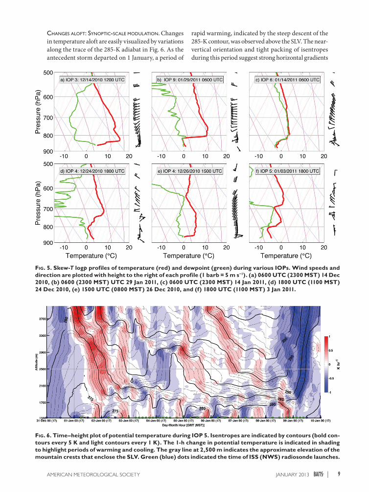
CHANGES ALOFT: SYNOPTIC-SCALE MODULATION. Changes in temperature aloft are easily visualized by variations along the trace of the 285-K adiabat in Fig. 6. As the antecedent storm departed on 1 January, a period of

rapid warming, indicated by the steep descent of the 285-K contour, was observed above the SLV. The near-vertical orientation and tight packing of isentropes during this period suggest strong horizontal gradients

FIG. 5. Skew-T logp profiles of temperature (red) and dewpoint (green) during various IOPs. Wind speeds and direction are plotted with height to the right of each profile (1 barb = 5 m s−1). (a) 0600 UTC (2300 MST) 14 Dec 2010, (b) 0600 (2300 MST) UTC 29 Jan 2011, (c) 0600 UTC (2300 MST) 14 Jan 2011, (d) 1800 UTC (1100 MST) 24 Dec 2010, (e) 1500 UTC (0800 MST) 26 Dec 2010, and (f) 1800 UTC (1100 MST) 3 Jan 2011.

FIG. 6. Time–height plot of potential temperature during IOP 5. Isentropes are indicated by contours (bold con-tours every 5 K and light contours every 1 K). The 1-h change in potential temperature is indicated in shading to highlight periods of warming and cooling. The gray line at 2,500 m indicates the approximate elevation of the mountain crests that enclose the SLV. Green (blue) dots indicated the time of ISS (NWS) radiosonde launches.


in vertical motion, consistent with localized subsid-ence found along the back edge of upper-level troughs. The combination of continued subsidence and in-creased differential warm-air advection is reflected by the continued descent of the 285-K isentrope into the SLV during the subsequent 24 h. As the region of warming and strong stability entered the upper reaches of the valley atmosphere, it formed a capping inversion layer and effectively initiated the CAP late on 1 January. The 285-K adiabat subsequently became horizontal during 2–3 January, which may result from differential vertical motion concentrating and tilting the potential temperature gradient within the elevated inversion layer.

A weak trough moved across the region on 4 January and led to a period of cooling aloft. Correspondingly, the 285-K isentrope ascended rapidly. The cooling and elevated mixing along the top edge of the inversion weakened but did not destroy the CAP. Warming aloft resumed by the next day (5 January), restoring and then augmenting the capping inversion. From 6 to 8 January, strong anticyclonic f low above the CAP generated a pro-longed period of warming throughout the lower and midtroposphere because of a combination of advec-tion and subsidence.

Beginning late on 8 January, a cold upper-level trough and associated arctic front approached the

region from the north. Cold-air advection and synoptic-scale ascent rapidly cooled the atmosphere above the valley, effectively “peeling back” the top of the CAP. The midtropospheric cold front arrived on 9 January and completely removed all of the remaining ambient stability, bringing an end to IOP 5. Despite the robust upper-level baroclinicity, the change in surface temperature during the frontal passage was negligible because of the cold air within the CAP.

BOUNDARY LAYER EVOLUTION. Boundary layer processes also contribute to the CAP evolution during IOP 5 (Fig. 7). Diurnal variations in the net radiation at the surface (Fig. 7b) contribute to alternating nocturnal surface inversions and daytime convective boundary layers, which are identified by the near-surface dome-shaped patterns in potential temperature (Fig. 7a). These diurnal variations in thermodynamic structure take place beneath the synoptically evolving stable layers aloft.

The strongest nocturnal surface inversions occur during clear nights (1, 2, 5, and 6 January), while weaker near-surface stratification is observed when clouds, either aloft or within the boundary layer, limit radiational cooling. For example, weak surface inversions, less negative net radiation, and greater mixing are observed on the nights of 3 and 4 January

FIG. 7. Aerosol, hydrometeor, and surface meteorological observations during IOP 5. (a) Laser ceilometer backscatter (color scale) and potential temperature (contours, as in Fig. 6a). (b) Net radiation from the ISFS 5 location. Near-surface vector winds with colors indicating wind speed (m s−1) at (c) Parley’s Canyon, (d) ISFS 3, and (e) ISFS 7.

10 JANUARY 2013|

when thin altostratus c louds , appa rent as strong returned power from the laser ceilom-eter, are present near the mountain-top level (Fig. 7a). The ceilom-eter also indicates the formation of stratiform boundary layer clouds overnight on both 7 and 8 January. Following a n in it ia l per iod of rad iat iona l cool i ng during the evening, these clouds form near the interface between t he c a p pi n g s t a b l e layer and the decaying convective boundary layer. In both instances, the cloud base lowers through the night with sur face fog forming during the predawn hours. Similar to the sounding in Fig. 5b, t he t hermody na mic structure during these nights indicates a moist adiabatic layer topped by a sharp inversion. On 8 January, the com-bination of cloud-top radiative cooling with synoptic-scale warming aloft yields a potential tem-perature deficit of ~25 K, the strongest deficit during PCAPS. Of note, hourly PM2.5 concentrations in excess of 90 μg m−3 were observed during this period (not shown).

An additional striking feature of the boundary layer evolution during IOP 5 is the vertical and tem-poral distribution of aerosol, which is indicated by higher levels of backscatter near the surface in Fig. 7a. Taken within the context of the potential tempera-ture structure (Fig. 7a, contours) and net radiation (Fig. 7b), it is apparent that aerosol depth and con-centration vary diurnally. The maximum aerosol depth tends to occur in the evening [0000 UTC (1700 MST)], which lags from the time of maximum heating, while the minimum depth occurs overnight. Careful examination of Fig. 7a indicates that aerosols are found within the stable layers aloft, which suggests

that circulations within the CAP, generated in part by diurnally varying slope and valley thermal flows, may contribute to the three-dimensional transport of aerosols. However, the f low within the valley is very complex, with some locations showing clear diurnal wind signatures (Fig. 7c), while others indi-cate varying flow patterns (Fig. 7d) or even periods of interbasin exchange (Fig. 7e).

CAP mix out. Pseudowarm fronts are sometimes observed during the breakup phase of CAPs (Whiteman et al. 2001). Referred to as mix out by local forecasters, such events are known to occur within the SLV when strong winds preceding an approaching storm interact with a CAP. PCAPS IOP 1 provided an excellent example of this phenomenon (Fig. 8). Strong southerly f low developed above the CAP as a synoptic-scale trough approached the region.

FIG. 8. Surface meteorological observations of the CAP displacement during strong southerly winds on 3 Dec 2010. The warm (cold) pseudofront position is indicated as red (blue) lines. Station observations are indicated by circular markers and shaded to correspond to the observed air temperature. Vectors indicate wind speed and direction. (a) 0200 UTC (1900 MST), (b) 0400 UTC (2100 MST), (c) 0500 UTC (2200 MST), (d) 0600 UTC (2300 MST), (e) 0800 UTC (0100 MST), and (f) 0900 UTC (0200 MST). (g) Air temperature (°C) and (h) vector winds (m s–1) at ISS site, which is emphasized with a magenta outline.


Southerly winds were observed to first penetrate to the surface along the southern and western portions of the valley, displacing the CAP to the north (Fig. 8a). The boundary between the cold, moist air within the CAP and the warm, dry, and mechanically mixed air to the south form a pseudowarm front. This boundary progressed northward throughout the night as winds aloft increased (Fig. 8b). By 0600 UTC, the warm front passed over the ISS site, providing a burst of strong southerly winds (Fig. 8h) and a rapid jump in temperature (Fig. 8g). Two hours later, as the weak trough passed over the region, the CAP returned southward now as a pseudocold front (Figs. 8d,e). Temperatures returned to their previous values accompanied by northerly winds. By 1400 UTC, the cold front propagated south through the entire valley, restoring CAP conditions to all locations (Fig. 8e).

SUMMARY AND FUTURE RESEARCH. The Persistent Cold-Air Pool Study (PCAPS), conducted in Utah’s Salt Lake valley, provides observations of the meteorological processes affecting the life cycle of persistent CAPs. During the 2-month-long field campaign, 10 intensive observation periods yielded a dataset that includes ~250 radiosonde observa-tions, continuous profiles of wind and temperature, boundary layer characterization, numerous surface meteorological observations, and energy budget mea-surements. This dataset (available at http://pcaps.utah .edu) provides a foundation for detailed analyses and numerical experiments related to persistent CAPs.

Initial analysis of data collected during PCAPS demonstrates a coherent link between strong long-lived CAPs and high concentration of fine particu-late aerosol. Silcox et al. (2012) further explore this relationship, finding a dependence of PM2.5 not only on CAP strength but also on altitude. Work underway will elaborate on these findings, both within the PCAPS period and over a broader clima-tological span. Researchers are also examining the deposition of particulate pollution and variations in carbon dioxide concentrations during persistent CAP events.

Not surprisingly, our initial analyses demonstrate the complexity of CAP evolution, with changes in CAP structure arising because of synoptic-scale advection and subsidence; mesoscale boundary layer flows; and radiative, turbulent, and cloud processes. Several research efforts are underway to directly target the relative role of these processes. For example, the high temporal and spatial resolution of the PCAPs data provides an opportunity to test theories for CAP removal due to regional pressure gradients (Zängl

2003) and turbulent erosion (Petkovsek 1978; Zhong et al. 2003). Additional investigations are targeting the role of thermally driven circulations within CAPs, including the impact of lake breezes and variations in land surface characteristics on CAP evolution. We also expect that this dataset will serve as the basis for numerical modeling of the PCAPS IOPs, an effort to be lead by scientists at the University of Michigan. This work will help to establish the com-parative importance of processes occurring at large and small scales and may improve forecasts for these high-impact events.

In addition to these targeted research topics, many more questions remain as to the evolution of persistent CAPs. One such example is the difficult to forecast transition between cloud-free and cloud-filled CAPs (R. Graham and L. Dunn, NWS, 2010, personal communication). We hope that the PCAPS dataset will serve as a resource for members of the meteorological and air quality research communi-ties interested in addressing problems pertaining to persistent CAPs.

ACKNOWLEDGMENTS. The NCAR Earth Observing Laboratory (EOL) provided field and data processing support from their ISS and ISFS groups. We greatly appreciate the many contributions of the EOL staff. Other PCAPS participating agencies included the Utah Division of Air Quality, the Utah Department of Transportation, the National Weather Service Forecast Office, Dugway Proving Ground, and Kennecott Utah Copper. University of Utah faculty members Geoff Silcox (Chemical Engineering) and David Bowling (Biology) operated a line of PM2.5 sensors and a network of snow samplers, respectively. Andrew Oliphant and Craig Clements of San Francisco and San Jose State Universities operated a f lux tower and micro-wave radiometer, respectively. We greatly appreciate the assistance of our University of Utah colleagues: Joe Young, Chris Anders, Roger Akers, and Chris Galli. Thanks are given to the 50 volunteers who donated their time to facilitate PCAPS operations. This research is supported pri-marily by Grant ATM-0938397 and secondarily by Grant ATM-0802282 from the National Science Foundation.

REFERENCESBaker, K. R., H. Simon, and J. T. Kelly, 2011: Challenges

to modeling “cold pool” meteorology associated with high pollution episodes. Environ. Sci. Technol., 45, 7118–7119.

Baklanov, A. A., and Coauthors, 2011: The nature, theory, and modeling of atmospheric planetary boundary layers. Bull. Amer. Meteor. Soc., 92, 123–128.

12 JANUARY 2013|

Chen, Y., F. L. Ludwig, and R. L. Street, 2004: Stably stratified flows near a notched transverse ridge across the Salt Lake valley. J. Appl. Meteor., 43, 1308–1328.

Clements, C. B., C. D. Whiteman, and J. D. Horel, 2003: Cold-air-pool structure and evolution in a mountain basin: Peter Sinks, Utah. J. Appl. Meteor., 42, 752–768.

Daly, C., D. R. Conklin, and M. H. Unsworth, 2009: Local atmospheric decoupling in complex topogra-phy alters climate change impacts. Int. J. Climatol., 30, 1857–1864.

Doran, J. C., J. D. Fast, and J. Horel, 2002: The VTMX campaign. Bull. Amer. Meteor. Soc., 83, 537–551.

Fernando, H. J. S., and J. C. Weil, 2010: Whither the stable boundary layer? Bull. Amer. Meteor. Soc., 91, 1475–1484.

Gillies, R. R., S.-Y. Wang, and M. R. Booth, 2010: Atmo-spheric scale interaction on wintertime intermoun-tain west low-level inversions. Wea. Forecasting, 25, 1196–1210.

Horel, J., and Coauthors, 2002: MesoWest: Cooperative mesonets in the western United States. Bull. Amer. Meteor. Soc., 83, 211–225.

Kondo, J., T. Kuwagata, and S. Haginoya, 1989: Heat budget analysis of nocturnal cooling and daytime heating in a basin. J. Atmos. Sci., 46, 2917–2933.

Malek, E., T. Davis, R. S. Martin, and P. J. Silva, 2006: Meteorological and environmental aspects of one of the worst national air pollution episodes in Logan, Cache valley, Utah, USA. Atmos. Res., 79, 108–122.

Neff, W. D., and C. W. King, 1989: The accumulation and pooling of drainage flows in a large basin. J. Appl. Meteor., 28, 518–529.

Pataki, D. E., B. J. Tyler, R. E. Peterson, A. P. Nair, W. J. Steenburgh, and E. R. Pardyjak, 2005: Can carbon dioxide be used as a tracer of urban atmo-spheric transport? J. Geophys. Res., 110, D15102, doi:10.1029/2004JD005723.

—, D. R. Bowling, J. R. Ehleringer, and J. M. Zobitz, 2006: High resolution atmospheric monitoring of urban carbon dioxide sources. Geophys. Res. Lett., 33, L03813, doi:10.1029/2005GL024822.

Petkovsek, Z., 1978: Turbulent dissipation of cold air lake in a basin. Meteor. Atmos. Phys., 47, 237–245.

Pinto, J. O., D. B. Parsons, W. O. J. Brown, S. Cohn, N. Chamberlain, and B. Morley, 2006: Coevolution of down-valley flow and the nocturnal boundary layer in complex terrain. J. Appl. Meteor. Climatol., 45, 1429–1449.

Price, J. D., and Coauthors, 2011: COLPEX: Field and numerical studies over a region of small hills. Bull. Amer. Meteor. Soc., 92, 1636–1650.

Reddy, P. J., D. E. Barbarick, and R. D. Osterburg, 1995: Development of a statistical model for forecasting

episodes of visibility degradation in the Denver metropolitan area. J. Appl. Meteor., 34, 616–625.

Reeves, H. D., and D. J. Stensrud, 2009: Synoptic-scale flow and valley cold pool evolution in the western United States. Wea. Forecasting, 24, 1625–1643.

—, K. L. Elmore, G. S. Manikin, and D. J. Stensrud, 2011: Assessment of forecasts during persistent valley cold pools in the Bonneville basin by the North American Mesoscale model. Wea. Forecasting, 26, 447–467.

Si lcox, G. D., K. E. Kel ly, E. T. Crosman, C. D. Whiteman, and B. L. Allen, 2012: Wintertime PM2.5 concentrations in Utah’s Salt Lake valley during per-sistent, multi-day cold-air pools. Atmos. Environ., 46, 17–24.

U.S. EPA, cited 2011: National Ambient Air Quality Standards (NAAQS). [Available online at www.epa .gov/air/criteria.html.]

Utah Asthma Program, 2010: Asthma and air pollution: Associations between asthma emergency department visits, PM 2.5 levels, and temperature inversions in Utah. Utah Department of Environmental Quality, 29 pp. [Available online at www.cleanair.utah.gov /health_presentations/docs/Asthma_Air_Pollution .pdf.]

Whiteman, C. D., X. Bian, and S. Zhong, 1999: Wintertime evolution of the temperature inversion in the Colorado plateau basin. J. Appl. Meteor., 38, 1103–1117.

—, S. Zhong, W. J. Shaw, J. M. Hubbe, X. Bian, and J. Mittelstadt, 2001: Cold pools in the Columbia basin. Wea. Forecasting, 16, 432–447.

—, and Coauthors, 2008: METCRAX 2006: Meteoro-logical experiments in Arizona’s Meteor Crater. Bull. Amer. Meteor. Soc., 89, 1665–1680.

Wolyn, P. G., and T. B. McKee, 1989: Deep stable layers in the intermountain western United States. Mon. Wea. Rev., 117, 461–472.

Zängl, G., 2002: An improved method for computing horizontal diffusion in a sigma-coordinate model and its application to simulations over mountainous topography. Mon. Wea. Rev., 130, 1423–1432.

—, 2003: The impact of upstream blocking, drainage flow and the geostrophic pressure gradient on the persistence of cold-air pools. Quart. J. Roy. Meteor. Soc., 129, 117–137.

Zhong, S., C. D. Whiteman, X. Bian, W. J. Shaw, and J. M. Hubbe, 2001: Meteorological processes affecting the evolution of a wintertime cold air pool in the Columbia basin. Mon. Wea. Rev., 129, 2600–2613.

—, X. Bian, and C. D. Whiteman, 2003: Time scale for cold-air pool breakup by turbulent erosion. Meteor. Z., 12, 229–233.


ABSTRACT

The Persistent Cold-Air Pool Study (PCAPS) was conducted in Utah’s Salt Lake valley

from 1 December 2010 to 7 February 2011. The field campaign’s primary goal was to improve

understanding of the physical processes governing the evolution of multiday cold-air pools

(CAPs) that are common in mountain basins during the winter. Meteorological instru-

mentation deployed throughout the Salt Lake valley provided observations of the processes

contributing to the formation, maintenance, and destruction of 10 persistent CAP episodes.

The close proximity of PCAPS field sites to residences and the University of Utah campus

allowed many undergraduate and graduate students to participate in the study.

Ongoing research, supported by the National Science Foundation, is using the PCAPS

dataset to examine CAP evolution. Preliminary analyses reveal that variations in CAP

thermodynamic structure are attributable to a multitude of physical processes affecting

local static stability: for example, synoptic-scale processes impact changes in temperatures

and cloudiness aloft while variations in boundary layer forcing modulate the lower levels

of CAPs. During episodes of strong winds, complex interactions between the synoptic and

mesoscale flows, local thermodynamic structure, and terrain lead to both partial and com-

plete removal of CAPs. In addition, the strength and duration of CAP events affect the local

concentrations of pollutants such as PM2.5.

14 JANUARY 2013|

the persistent cold-air pool study

Documents