Research Division Federal Reserve Bank of St. Louis Working Paper Series

The Perils of Globalization: Offshoring and Economic Insecurity of the American Worker

Richard G. Anderson and

Charles S. Gascon

Working Paper 2007-004A http://research.stlouisfed.org/wp/2007/2007-004.pdf

February 2007

FEDERAL RESERVE BANK OF ST. LOUIS Research Division

P.O. Box 442 St. Louis, MO 63166

______________________________________________________________________________________

The views expressed are those of the individual authors and do not necessarily reflect official positions of the Federal Reserve Bank of St. Louis, the Federal Reserve System, or the Board of Governors.

Federal Reserve Bank of St. Louis Working Papers are preliminary materials circulated to stimulate discussion and critical comment. References in publications to Federal Reserve Bank of St. Louis Working Papers (other than an acknowledgment that the writer has had access to unpublished material) should be cleared with the author or authors.

The Perils of Globalization:

Offshoring and Economic Insecurity of the American Worker

Richard G. Anderson*

Charles S. Gascon†

February 2007

(version of February 9, 2007)

Abstract

According to polls from the 2006 congressional elections, globalization and economic insecurity were the primary concerns of many voters. These Americans apparently believe that they have fallen victim to liberal trade polices and that inexorable trends in globalization are destroying the American Dream. In this analysis, we use time series cross-section data from the General Social Survey (GSS) to examine the links among offshoring, labor market volatility, and the demand for social insurance. Unique among the GSS literature, our analysis includes a pseudo-panel model which permits including auxiliary state and regional macroeconomic information.

Keywords: economic insecurity, globalization, labor-demand elasticity, offshoring,

JEL classification: F16; J23; C23

* Economist and Vice President, Federal Reserve Bank of St. Louis † Research Associate, Federal Reserve Bank of St. Louis

Views expressed are the authors and are not necessarily those of the Federal Reserve Bank of St. Louis, the Board of Governors or the Federal Reserve System.

1 Introduction

Polls from the 2006 congressional elections placed globalization and economic insecurity

as the driving forces behind the large economic populist vote, and found that 40 percent

of Americans think the next generation will have a lower standard of living than today.

Moreover, 62 percent said there was less job security and 59 percent said they had to

work harder to earn a decent living. Many Americans undoubtedly believe they have

fallen victim to liberal trade polices and that globalization is destroying the American

Dream: 75 percent said outsourcing work overseas hurts American workers.1

Conversely, most economists would argue the U.S. economy has been enriched

by increases in world trade. According to Bradford, Grieco and Hufbauer (2006),

globalization has brought an extra $800 billion to $1.4 trillion annual income (or about

$7,000 to $13,000 per household) to the United States since World War II. At the same

time, many economists have expressed concern regarding the uneven occupational,

regional, and industry-specific impact of increased trade: While the economy gains

overall, not everyone gains. Globalization is exposing a deep fault line between groups

who have the skills and mobility to flourish in global markets and those who either don’t

have these advantages or perceive the expansion of unregulated markets as inimical to

social stability and deeply held norms (Rodrik, 1997).

Globalization displaces workers and creates insecurities that increase the demand

for social insurance (Garrett, 1998; Rodrik, 1997). As a result, postwar globalization was

founded on the principle that the federal government would provide economic security,

while free international markets would provide the best aggregate outcomes. The search

naturally arises for a mechanism to “share” the gains from trade. Absent a suitable

political consensus, the objections or even the visibility of the harmed persons, regions,

and industries, threaten to derail and perhaps reverse reductions in trade barriers as they

have done in the past.

Kevin O’Rourke and Jeffery Williamson (1999) note that 19th century

globalization sowed the seeds of its own destruction. Political backlash due to economic

1For poll results and mass media reports on economic insecurity see Greenhouse (2006), Orszag (2006),Lynch (2006), or Summers (2006).

-1-

insecurity, not economic factors, killed globalization.2 Somewhat regrettably, postwar

changes in the economy are likely to have increased workers’ anxiety today, most notably

the significant change in the composition of traded goods and services.

Traditionally, trade is thought of as exchanging different goods across nations, not

the shifting of production from one country to another, followed by return shipments

back to the original country. For example, in the past, U.S. firms would export good x

and import good y. In the New Economy, U.S. firms export the capital k needed to

produce good x to a country with lower production costs and then re import good x.3

Theoretically, disaggregating the value chain has allowed U.S. business to substitute

cheaper foreign labor for domestic labor, increasing firms’ own price elasticity of

demand for labor, raising the volatility of wages and employment, which increase worker

insecurity.

This phenomenon of rising economic insecurity in developed nations during the

1990s (and now, as we will show, into the 2000s) has sparked widespread interest in its

causes and consequences. Past research suggests the implications of rising insecurity are

far-reaching: including wage restraint, ill health, reduction in consumer expenditure, and

economic inequality.4 There is a vast collection of literature examining the structural

determinates impacting perceptions of economic insecurity in the United States (e.g.,

Aaronson and Sullivan, 1998; Dominitz and Manski, 1997; Manski and Straub, 2000;

Schmidt, 1999). Unfortunately, empirical research explicitly connecting globalization to

increased economic insecurity is non-existent. This paper is the first, to our knowledge,

to empirically examine the forces of globalization—more specifically, offshoring— and

workers’ perceived economic insecurity in the United States.

In this article, we use 1977-20045 data from the General Social Survey (GSS) to

investigate if U.S workers have, in fact, become more pessimistic about their economic

2 O’Rourke and Williamson discuss three notable examples of globalization and its political backlash in the late 19th century (early 20th century): (1) cheap grain from the New World threatened agricultural incomes in Europe, leading to tariffs on agricultural imports from the New World; (2) mass immigration from Europe threatened New World living standards, escalating immigration restrictions in the New World; and (3) European manufactured exports threatened emerging industries in the New World, leading to high tariffs in the New World on European manufactured imports. 3 Some analysts have referred to this as a flattening of the world, others as disaggregating the value chain such that products, and components of manufactured products, are manufactured worldwide. 4 See Green, Felstead, and Burchell (2000) for a summary. 5 Data from the 2006 GSS will be available in early 2007, and we plan to update after that time..

-2-

security into the 21st century and, more specifically, whether offshoring has played a

significant role in fostering this insecurity. We build upon the work of Scheve and

Slaughter (2004), who examine the impact of foreign direct investment on economic

insecurity in Great Britain from 1991 to 1999. We find evidence suggesting that workers

in tradable industries and occupations express higher levels of economic insecurity;

additionally, workers expressing higher levels of insecurity demand greater social

insurance.

Our empirical work attempts to resolve some widely ignored issues in the GSS

literature. The GSS dataset consists of a time series of cross-section surveys, but not a

panel structure. In other words, we cannot follow individuals through time. However,

unique among such datasets, the GSS includes many responses per individual on related

(and unrelated) questions. Our estimation strategy is two fold. At the micro level we use

auxiliary information (responses to auxiliary survey questions) to remove (filter)

individual effects. Our second estimation strategy is one of cohort-specific effects, or,

specifically, regional macroeconomic analysis.

The paper is organized into the following sections. Section 2 reviews the

economic theory as it pertains to globalization. Section 3 describes our data. Section 4

presents our individual and cohort level empirical specification and analysis. Section 5

discusses policy implications and proposals. The final section concludes.

2 Theory

Economic insecurity is most often understood as an individual’s perception of the risk of

economic misfortune (Dominitz and Manski, 1997; Scheve-Slaughter, 2004). Economic

misfortune can be thought of as individuals’ inability to purchase goods and services (or

provide for their families), which primarily depends on their income. In reality, the

majority of Americans do not earn their primary income from dividend payments or stock

options, but rather from wages from labor income. Therefore, we assume that economic

insecurity primarily stems from volatility in wages and employment, caused by volatility

in the labor market. As a result, this section utilizes labor theory in conjunction with

trade theory to explain how offshoring affects economic insecurity via increases in

industries’ labor-demand elasticities.

-3-

2.1 Globalization and the elasticity of demand for labor

An industry’s own-price labor demand elasticity, ηjd

, consists of two parts, the scale effect

(sηj) and the substitution effect (–1[1–s]σj) so that ηjd

= –1[1–s]σj – sηj.6 The scale effect

tells us how much labor demand changes after a wage change due to a change in output.

The substitution effect tells us, for a given level of output, how much firms substitute

away from labor and toward other factors of production when wages rise. Both the scale

and substitution effects reduce the quantity of labor demanded when wages rise. For the

purpose of this paper, we focus on the processes in which offshoring increases labor-

demand elasticities via the substitution effect.7

Suppose an industry is vertically integrated with a number of production stages.

Trade allows domestic firms to lower production costs by offshoring work to foreign

businesses and importing intermediate inputs (e.g., Feenstra and Hanson, 1996, 1999).

Trade thus increases the number of factors that firms can substitute in response to higher

domestic wages beyond just domestic non-labor factors.8 Therefore, moves toward freer

trade should increase the elasticity of substitution, σj. Firms need not actually offshore

jobs to increase σj; the potential of offshoring is sufficient (Slaughter, 2001). As this

substitutability increases, labor demand becomes more elastic.9 Additionally, the smaller

s the stronger is the pass-through from σj to ηjd

. As a result, higher wages generate larger

changes in the quantity of labor demanded the less important labor is in total costs.10

6 Where s is labor’s share of industry total revenue; σj is the constant-output elasticity of substitution between labor and all other factors of production; and ηj is the product-demand elasticity for industry j’s output market. ηj

d is defined as negative; s, σj, and ηj are positive.

7 Scheve and Slaughter (2004) note several reasons for focusing on the substitution effect: first, because it is direct, that is, it places domestic workers in competition with foreign labor, and, second because other researchers (primarily Rodrik, 1997) have emphasized in theory its possible role in generating insecurity. 8 According to Freeman (2005), the opening of India, China, and the former Soviet bloc to international commerce during the 1990s approximately doubled the worlds supply of labor from 1.46 billion workers to 2.92 billion. However, these countries brought with them limited capital, dropping the global labor-to-capital ratio by approximately 40 percent, decreasing the returns to labor, and increasing the returns to capital. Based on the findings of Rauch and Trindade (2003), this massive increase in the labor supply in foreign nations has nearly equal proportionate effects as a domestic increase in labor supply on U.S. labor-demand elasticity, suggesting that without change in U.S trade policy, the increased openness in other nations will have the same effect on labor-demand elasticities.

9 0]1[ <−= sd

δσδη .

10 This is where the role of increasing automation affects labor-demand elasticities. Increases in automation will reduce s, increasing the pass-through effect. Replacing a worker with a computer will exacerbate the impact of trade on the labor-demand elasticity.

-4-

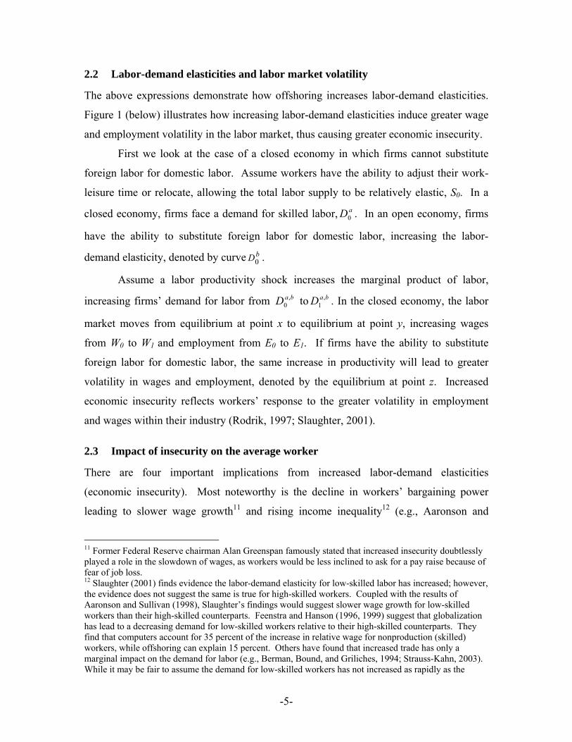
2.2 Labor-demand elasticities and labor market volatility

The above expressions demonstrate how offshoring increases labor-demand elasticities.

Figure 1 (below) illustrates how increasing labor-demand elasticities induce greater wage

and employment volatility in the labor market, thus causing greater economic insecurity.

First we look at the case of a closed economy in which firms cannot substitute

foreign labor for domestic labor. Assume workers have the ability to adjust their work-

leisure time or relocate, allowing the total labor supply to be relatively elastic, S0. In a

closed economy, firms face a demand for skilled labor, aD0 . In an open economy, firms

have the ability to substitute foreign labor for domestic labor, increasing the labor-

demand elasticity, denoted by curve bD0 .

Assume a labor productivity shock increases the marginal product of labor,

increasing firms’ demand for labor from baD ,0 to baD ,

1 . In the closed economy, the labor

market moves from equilibrium at point x to equilibrium at point y, increasing wages

from W0 to W1 and employment from E0 to E1. If firms have the ability to substitute

foreign labor for domestic labor, the same increase in productivity will lead to greater

volatility in wages and employment, denoted by the equilibrium at point z. Increased

economic insecurity reflects workers’ response to the greater volatility in employment

and wages within their industry (Rodrik, 1997; Slaughter, 2001).

2.3 Impact of insecurity on the average worker

There are four important implications from increased labor-demand elasticities

(economic insecurity). Most noteworthy is the decline in workers’ bargaining power

leading to slower wage growth11 and rising income inequality12 (e.g., Aaronson and

11 Former Federal Reserve chairman Alan Greenspan famously stated that increased insecurity doubtlessly played a role in the slowdown of wages, as workers would be less inclined to ask for a pay raise because of fear of job loss. 12 Slaughter (2001) finds evidence the labor-demand elasticity for low-skilled labor has increased; however, the evidence does not suggest the same is true for high-skilled workers. Coupled with the results of Aaronson and Sullivan (1998), Slaughter’s findings would suggest slower wage growth for low-skilled workers than their high-skilled counterparts. Feenstra and Hanson (1996, 1999) suggest that globalization has lead to a decreasing demand for low-skilled workers relative to their high-skilled counterparts. They find that computers account for 35 percent of the increase in relative wage for nonproduction (skilled) workers, while offshoring can explain 15 percent. Others have found that increased trade has only a marginal impact on the demand for labor (e.g., Berman, Bound, and Griliches, 1994; Strauss-Kahn, 2003). While it may be fair to assume the demand for low-skilled workers has not increased as rapidly as the

-5-

Sullivan, 1998). Second, increases in the elasticity of labor demand shift the costs of

benefits, such as healthcare, away from firms toward workers.13 Third, Benito (2006)

finds that increased insecurity causes households to defer consumption. Finally, Burchell

(1999) concludes that economic insecurity is damaging to workers’ health.

On the other hand, gains from globalization have been quite large and have taken

many different forms, specifically, lower prices, higher profits, and increased product

variety. Estimates by Bradford, Grieco and Hufbauer (2006) suggest that future gains

from removing the rest of U.S trade barriers could add at least another $1.3 trillion to the

U.S. economy annually.14 However, as previously mentioned, a large majority of workers

rely on wages from labor income, not profits, to provide for their families. While the

gains from globalization have been grand for the economy as a whole, when the average

worker constructs an opinion about the effect of globalization, the direct impact of

declining wages (real and relative) and increasing healthcare costs will likely outweigh

the more indirect benefits.

3 Variables to capture the peril of globalization

Our empirical work seeks to examine how workers’ perceptions of their economic

insecurity are affected if they work in industries (or occupations) that are susceptible to

offshoring. Our data are from the General Social Survey (GSS) conducted by the

National Opinion Research Center of the University of Chicago. The survey is

administered in February and March of each sample year, with the total number of

respondents ranging from 1,468 to 2,832. Since 1994, the GSS has been conducted on a

biannual basis. Respondents answer questions regarding their demographic information

and opinions on a plethora of topics, including two questions about earnings and

employment expectations. These questions were included in 17 surveys between 1977

and 2004. We use the responses from these two questions to measure economic

insecurity. So far as we are aware, this is the only large survey dataset for the United

States that contains such questions.

demand for high-skilled workers, rising insecurity (labor-demand elasticities) can explain an increasing income gap between high- and low-skilled workers within and across industries. 13 See Rodrik (1997) p.18 for a complete discussion. 14 The authors believe this may be an underestimate, perhaps by a great deal.

-6-

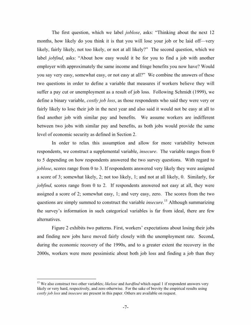
The first question, which we label joblose, asks: “Thinking about the next 12

months, how likely do you think it is that you will lose your job or be laid off—very

likely, fairly likely, not too likely, or not at all likely?” The second question, which we

label jobfind, asks: “About how easy would it be for you to find a job with another

employer with approximately the same income and fringe benefits you now have? Would

you say very easy, somewhat easy, or not easy at all?” We combine the answers of these

two questions in order to define a variable that measures if workers believe they will

suffer a pay cut or unemployment as a result of job loss. Following Schmidt (1999), we

define a binary variable, costly job loss, as those respondents who said they were very or

fairly likely to lose their job in the next year and also said it would not be easy at all to

find another job with similar pay and benefits. We assume workers are indifferent

between two jobs with similar pay and benefits, as both jobs would provide the same

level of economic security as defined in Section 2.

In order to relax this assumption and allow for more variability between

respondents, we construct a supplemental variable, insecure. The variable ranges from 0

to 5 depending on how respondents answered the two survey questions. With regard to

joblose, scores range from 0 to 3. If respondents answered very likely they were assigned

a score of 3; somewhat likely, 2; not too likely, 1; and not at all likely, 0. Similarly, for

jobfind, scores range from 0 to 2. If respondents answered not easy at all, they were

assigned a score of 2; somewhat easy, 1; and very easy, zero. The scores from the two

questions are simply summed to construct the variable insecure.15 Although summarizing

the survey’s information in such categorical variables is far from ideal, there are few

alternatives.

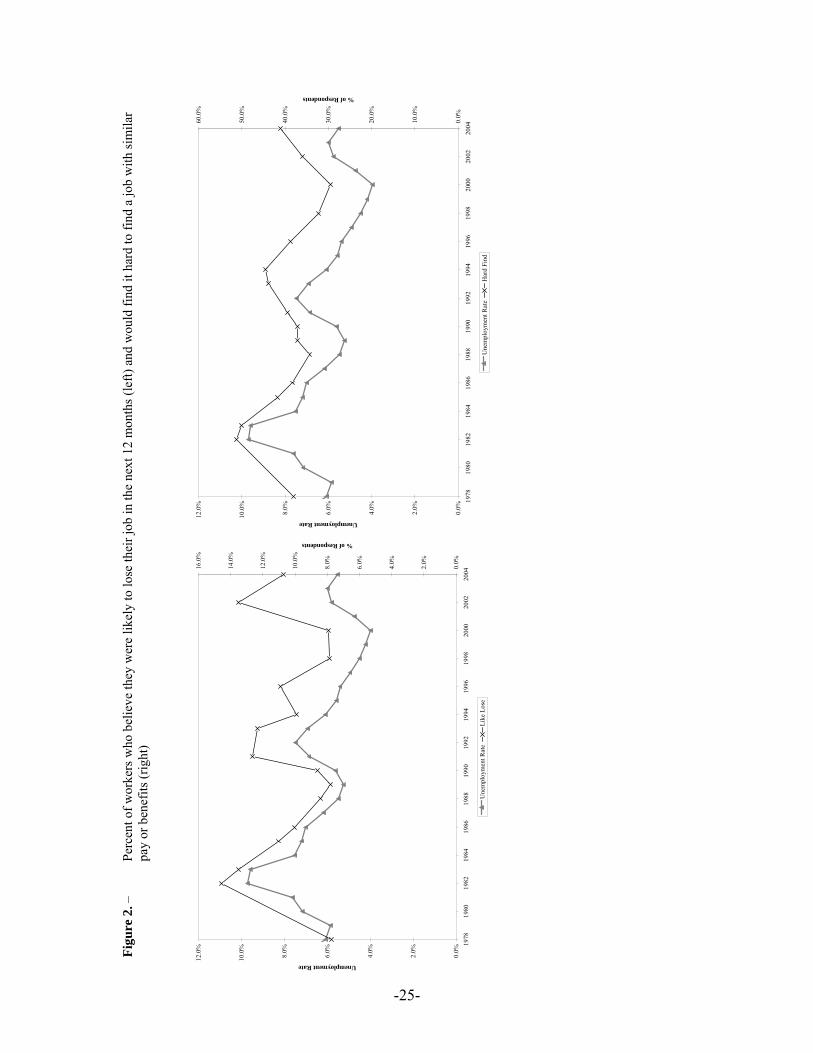
Figure 2 exhibits two patterns. First, workers’ expectations about losing their jobs

and finding new jobs have moved fairly closely with the unemployment rate. Second,

during the economic recovery of the 1990s, and to a greater extent the recovery in the

2000s, workers were more pessimistic about both job loss and finding a job than they

15 We also construct two other variables; likelose and hardfind which equal 1 if respondent answers very likely or very hard, respectively, and zero otherwise. For the sake of brevity the empirical results using costly job loss and insecure are present in this paper. Others are available on request.

-7-

were during the previous periods of low unemployment in the 1970s and 1980s, as

highlighted by the growing divergence with the unemployment rate.16

Our theory hypothesizes that tradable industries (and occupations) will exhibit

more-elastic labor demands, which, raises labor-market volatility. According to the

findings of Jensen and Kletzer (2005), this is exactly the case. Tradable industries have

job-loss rates that are notably higher than those safe from offshoring: 0.152 compared

with 0.076. Moreover, occupations exposed to global trade exhibited higher rates of job

loss than safe occupations: 0.22 compared with 0.094. Additionally, workers in tradable

industries saw income (in logs) loss of -0.30 compared with -0.14 in non tradable

industries. Therefore, we expect workers in industries and occupations safe from

offshoring to express significantly lower levels of economic insecurity. Following the

results of Jensen and Kletzer, we construct our offshoring variables.17

To develop an empirical approach to identify activities that can be potentially

offshored, Jensen and Kletzer assume activities traded domestically can be potentially

traded internationally, even if they currently are not. Using spatial clustering, they group

industries and occupations into “Gini classes,” where those industries and occupations

with Gini coefficients less than 0.1 are classified as “Gini class 1” or non tradable. We

base our construction of our two offshoring variables on their results.18 The variable

pIND identifies those industries in which activities can be offshored. Industries such as

personal services (e.g., teeth cleaning) are coded as zero, or non tradable. There is no

reason a dentist or hygienist would worry about their job being offshored. Other

industries in which the work could feasibly be offshored are coded as one.

Similar to offshoring threats by industry, certain occupational groups are directly

or indirectly affected by offshoring. Some workers may find themselves in industries

where they are safe from offshoring but are in an occupation in which employees in

similar jobs in different industries are being offshored. Such is the case with

administrative support positions. An administrative assistant at a dentist’s office may not

16 The first and to some extent the second patterns were previously recognized by Schmidt (1999). 17 See Jensen and Kletzer (2005) for further discussion of the methodology used to identify tradable industries and occupations. 18 The GSS reports respondents’ Census industry and occupations codes, while Jensen and Kletzer use NACIS and Major Standard Occupations Classification codes; therefore we use our best judgment to apply their results. See Table 1 for comparative figures.

-8-

fear that his job will be offshored, but if he does lose his job it may be harder for him to

find a new job because other industries have been able to offshore this work. We

construct a variable pOC to identify those occupational groups that are safe from

offshoring. Occupations safe from offshoring (e.g., judges or physicians) are coded as 0;

those that can be offshored are coded as 1. Using these two variables exploits the fact that

respondents provide information on their industries as well as their occupations within

their respective industries.19

Workers’ perceptions about their economic security are formed by many

characteristics beyond the pressures from offshoring. Consequently, we construct a

number of individual-level control variables.20 The variable Income is a categorical

variable measuring real household income.21 Union equals 1 if the respondent belongs to

a union, and 0 if not. Degree is a categorical variable ranging from 1 to 5, with 1 the

lowest education and 5 the highest. AgeGr is a vector of binary variables corresponding

to respondents’ respective age group at the time of the survey. White, Black, and Other

equal 1 if the respondent identifies as white, black, or other, respectively, and 0

otherwise. Self equals 1 if the respondent identifies himself as being self-employed and 0

otherwise. Region is a vector of nine binary variables corresponding to the nine Census

divisions.22 Unemployment measures the share of workers unemployed in a respondent’s

census region during the survey year.23 Finally, Year is a vector of binary variables

controlling for year fixed effects.

19 In addition to the potential for offshoring, the magnitude of offshoring activity within an industry (or region) may be of some importance. Higher levels of offshoring activity could indicate greater mobility, which in turn raises labor-demand elasticities and perceptions of employment risks (Scheve and Slaughter, 2004). However, U.S regional import data per se are not available (see Hervey, 1999), nor is Foreign Direct Investment (FDI) data by industry classification at comparable levels of disaggregation. Moreover Scheve and Slaughter construct an FDI magnitude variable that produces coefficients that are not statistically different from their potential coefficients at a 95percent confidence level. 20 See appendix table 6 for more information. 21 The GSS asks respondents to report their annual household income within equal nominal brackets that arbitrarily change over time. The values range from 1 for the lowest income bracket to 9 for the highest income bracket. We compute the annual median value and use the deviation from the median value as a proxy for real household income, (e.g. If in year y, the median respondent, I, reported his family income to be in bracket 4 then respondent i's real family income was coded as zero. If respondent i+1 reported to have a family income for year, y in bracket 5, i+1’s real family income is coded as 1). 22 If respondent lives in the respective Census region at the time of the survey, they are assigned a value of 1, and 0 otherwise. We will later use this information for our cohort analysis. 23 These data were obtained from the Bureau of Labor Statistics (BLS).

-9-

The control variables are likely to account for some of the variation among

individuals’ perceptions about their economic security. However, individual-specific

immeasurable and/or unobserved differences may also matter. When answering the GSS

survey question about finding a new job, one respondent may believe he could find a new

job paying 10 percent less with comparable benefits and answer “somewhat easy”, while

another respondent may be in the same situation and say “not easy at all.” Unlike the

U.K. panel survey data used by Scheve and Slaughter, the GSS is a time series of cross-

sections that does not track the same individual over different years. We are unable to

control for individual-specific effects using the standard practice.24 We use auxiliary data

from the GSS survey to approximate the existing individual bias.

The GSS asks respondents a question about their past financial situation and

general happiness, specifically: “During the last few years, has your financial situation

been getting better, worse, or has it stayed the same? Taken all together, how would you

say things are these days—would you say that you are very happy, pretty happy, or not

too happy?” We code the respondents’ answers to these questions with values ranging

from 1 to 3, where 3 equals getting better and very happy. Using this coding, we

construct the variables fSit and gHap.

Including these variables in our models allows us to approximate unobserved

effects that influence the respondents’ answers to the economic insecurity questions.

More specifically, fSit can be thought of as a proxy for a lagged dependent variable, as

respondents’ past financial situation’s will likely influence their future outlook. The

gHap variable can be thought of as a bias correction, as generally happy people are more

likely to be optimistic when expressing their perceptions of economic security.25

Including these variables in our estimation produces more precise estimates, but by no

means accounts for all the unobserved individual effects that are possible in a panel

structure.

24 Starting in 2008 the GSS will switch from a repeating cross-section design to a combined repeating cross-section and panel-component design. When these new data become available they will allow future research to test our approach of controlling for individual-specific effects. 25 There is clearly an endogeneity issue between general happiness and economic security that we correct for using IVmethods. Survey questions on martial status, occupational happiness, financial satisfaction, and friendship happiness are reserved to satisfy identification restrictions.

-10-

4 Empirical specification, estimates and analysis

In section 4.1, we analyze the pooled cross-section time-series GSS data using ordered

probit models, so as to examine the variation in our measures of economic insecurity at

the individual-respondent level. In section 4.2, we stratify the data by Census region and

estimate a Deaton-style “pseudo-panel” model to examine economic insecurity at a more

macroeconomic regional level. Among other advantages, this framework allows us to

replace certain macroeconomic variables used in the individual-respondent model

(aggregated from the GSS dataset) with more satisfactory aggregate regional data from

the Bureau of Economic Analysis.

4.1 Individual level

In cases where the variable to be estimated is limited to a range of values and contains

discrete responses, probit models are employed to provide the best estimation (e.g., coin

toss). As noted by Aaronson and Sullivan (1998), in cases where the underlying variable

(perceived economic insecurity) is continuous in nature but approximated by discrete and

ordered responses of a survey question, the appropriate statistical technique is the use of

ordered probit models. The ordered probit regression is based on a latent regression such

as *iy = βxi + εi, where *

iy is the unobserved economic insecurity of individual i, xi are

demographic and other individual characteristics of individual i, and εi is a person-

specific error term. The parameter β is a vector of coefficients to be estimated. Although

we do not observe *iy , we observe k possible answers allowed by the survey and the

construction of our insecurity measures, as represented by yi:

yi =0 if *iy ≤µ0

yi =1 if µ0≤ *iy ≤µ1

yi =2 if µ1≤ *iy ≤µ2

. . . yi = k if µk-1≤ *

iy .

For example, for the costly job loss variable, yi=1 corresponds to answering

“somewhat likely” or “very likely” and “very hard,” whereas for the insecure variable,

yi=5 corresponds to “very likely” and “very hard.” The µi’s are unknown intercept

parameters to be estimated.

-11-

Table 2 reports the coefficients and standard errors from specifications that use

costly job loss and insecure as dependent variables. The first three columns of the table

use costly job loss as the dependent variable and the last three columns use insecure. The

results are reported relative to a base-case white, female, non-union, age 25 to 39, who

lived in the northeast in 1988. The model fits well. The majority of the estimated

coefficients have the expected signs. A notable exception is the Union variable, which

has a positive and highly significant coefficient.26 The unobserved individual-effect

variables gHap and fSit have the largest impact on our insecurity variables. Our

potential-for-offshoring variables, pIND and pOC, are positive and significant across all

model specifications, supporting our hypothesis that employees in industries and

occupations safe from offshoring will express lower levels of job insecurity.

Assuming E(εi)=0 and V(εi)=σ2, we can calculate the base case probability of each

of the k answers.

Φ(µ0 + βx) if j=0 Prob (y= j|x) = Φ(µ0 + βx) - Φ(µj-1 + βx) if 0 < j ≤k-1 1-Φ (µk-1 + βx) if j=k, where Φ is the standard normal cumulative distribution function. From the equation

above, we can calculate the marginal effects on the base case by

ββμφ )()0(0 x

xyprob

+=∂

=∂

ββμφβμφ ))()(()(1 xx

xjyprob

jj +−+=∂

=∂−

,))(1()(1 ββμφ x

xkyprob

k +−=∂

=∂−

where φ is the standard normal density function and the x variables are measured at their

mean value. In many cases, the independent variables are binary indicators, such as male

or white. In this case, the marginal effect is calculated as follows:

26 If we assume that union membership is, in fact, exogenously determined, this coefficient suggests that by joining a union the respondent will express higher levels of job insecurity. Theoretically this does not make much sense, as workers join unions to increase their job security. On the other hand, the natural decline of union membership in the United States and higher union wages means that if union members do lose their job it is very likely they will experience a pay cut. See Bender and Sloane (1999) for further discussion.

-12-

Prob (y= j|x´,1) – Prob (y= j|x´,0), where x´, 1 is the vector of covariates where the male (white) variable is set to 1 and x´, 0

is the vector of covariates where the male (white) variable is set to 0.

The base-case probabilities and marginal effects, in Table 3, measure the impact

of a change in the respective independent variable on the probability of the respondent

expressing a certain level of job insecurity. For example, for every unit increase in the

regional unemployment rate, the probability of expressing costly job loss increases 0.56

percent, all else constant. The first row of this table shows that the probability of the

base-case person expressing costly job loss is 6.2 percent.

With respect to our offshoring variables, pInd and pOC, the probability the base-

case worker will express costly job loss if she works in an industry and occupation with

the potential for offshoring increases to about 8.5 percent, from 6.2 percent. The

individual-effect variables play even a greater role in predicting workers’ economic

insecurity. Specifically, the probability that the base-case respondent will express costly

job loss is only about 2 percent if they are “very happy” and have seen their financial

situation improve over the past few years. The probability that the same base-case

respondent will express costly job loss is about 10 percent if they are “not too happy” and

have seen their financial situation get worse.

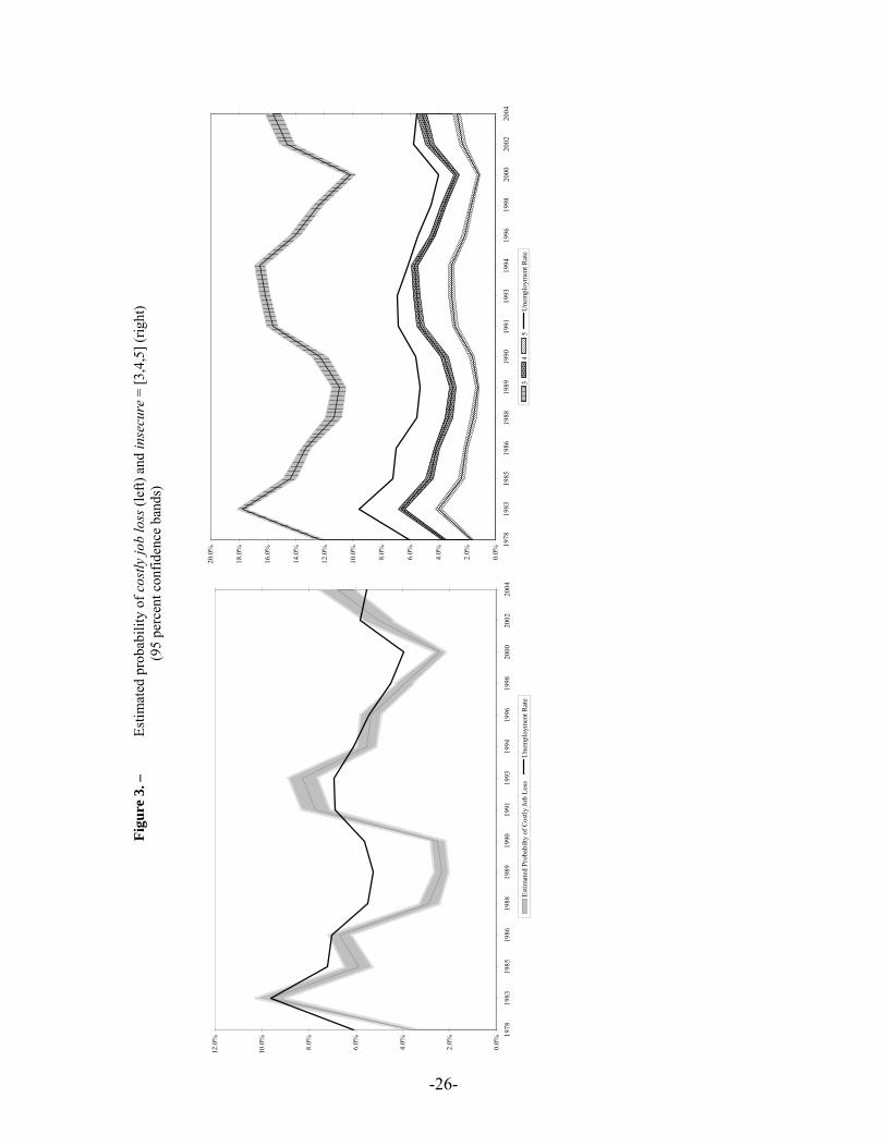
Figure 3 plots the estimated probabilities of costly job loss and insecure over the

sample period. As we expect, workers probability of expressing economic insecurity

moves in sync with fluctuations in the labor market, measured by the national

unemployment rate. However, in 2004 there is a significant departure from this trend,

suggesting that recent improvements in the labor market have not quelled economic

insecurity as they have in the past

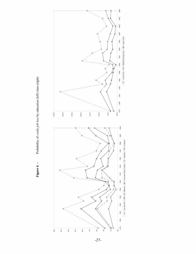
Breaking down the probabilities even further in Figure 4, we see that upper-class

workers have seen some reprieve from improvements in the labor market but

middle/working class and lower class workers continue to express heightened levels of

economic insecurity. Data since 2000, by education level show that workers across all

education levels are expressing higher levels of economic insecurity, with lower-educated

workers experiencing the starkest increases. Somewhat contrary to previous findings, our

-13-

results suggest that the economic growth of the 1990s eventually reduced workers

economic insecurity, although never to levels lower than those of the 1980s.

4.2 A Regional level, Pseudo-Panel Model

Above, we have conducted estimation with the pooled GSS dataset. Because the GSS is a

series of cross-sections and not a panel dataset, it is not possible to control for individual

effects nor to estimate a dynamic model that uses lagged dependent and independent

variables.27 Deaton (1985) introduced the concept of stratifying such datasets according

to certain exogenous variables, creating a “pseudo-panel” dataset. There are two

underlying assumptions needed to successfully convert the GSS data into a panel

structure. First, if there are individual-specific effects, there will be equivalent additive

cohort effects. Second, the sample cohort means are consistent estimates of the true

cohort means. Consider the simple theoretical model, itititit xy εβ += , where yit is the

measure of job insecurity of individual i at time t, xit is a vector of demographic

individual characteristics, β is a vector of parameters to be estimated, and ε is the error

term. In a normal panel structure, researchers track certain individuals over time,

allowing econometricians to use individuals as their own controls, or individual fixed-

effects, modeled as

itiitit xy εθβ ++= , (1)

where θi captures the individual fixed effect. Since θi will be correlated with other

explanatory variables, this equation can only be consistently estimated from panel data.

However, consider a case where i is a member of a well-defined cohort monitored

through successive surveys. Let i belong to a cohort, c, and calculate the simple

population averages of (1) over all i belonging to c to obtain

****ctcctct xy εθβ ++= , (2)

27 Our variables gHap and Fsit appear to be fair approximations of these individual effects; that is to say, they are powerful predictors of economic insecurity.

-14-

where the asterisks denote population means. In practice, these cohort population means

can be estimated by cohort means from the sample. We then get sample cohort means,

forming the relationship

ctctctct xy_____εθβ ++= , (3)

where ct_θ is the average of the fixed effects for those i part of c that show up in the

survey. 28

Deaton’s work considered only static panel models, but later econometric studies

have examined the possibility of estimating dynamic pseudo-panel models. The

necessary conditions for consistent estimation of such models are stringent and, in our

opinion, unlikely to be fulfilled in most non-panel survey datasets; see for example

Verbeek and Vella (2005).29 Hence, we do not pursue dynamic pseudo-data panel

models.

Following Deaton’s methodology, we group our data into regional cohorts

corresponding to the nine census regions, reducing the total observations in the sample to

153. Averaging our individual dummy variables produces regional composition

measures, (i.e., 50 percent of the sample is male). Due to the reduction in observations

and the large number of regressors, we estimate the following fixed-effects model to

preserve degrees of freedom:

ctcctctcct xxyy______

)( εβ +−=− , (4)

where cy_

and cx_

are the means of each regional cohort over all sample years.

Grouping the GSS data into regional cohorts allows us to replace certain state and

local variables created via aggregation of GSS survey questions with more satisfactory

(in our opinion) state and regional data from the Census Bureau and BEA. For example, a

measure of real household income is included on GSS dataset; in the pseudo-panel

28 After conducting data sampling tests, we assume ct

_θ = *

cθ . Note: The GSS is not a random sample, and we lose some observations due to question availability; therefore, we use information from other sources to test if the cohort sample means equal the cohort means of other data sources. For example, we use regional cohorts, and the Bureau of Economic Analysis (BEA) provides employment data by region. Amongst other things we test if the distribution of employment between regional cohorts is equal to the true employment distribution reported by the BEA. See appendix table A.2 for results. 29 Other papers discussing dynamic pseudo-panel models include Moffit (1993) and Collado (1997).

-15-

models, we can use BEA estimates of real per capita personal income.30 To check

robustness, we estimate our models with both the GSS and BEA measures.31 Further,

the GSS race classifications of white, black, and other are not statistically representative

of the regional demographic mix; therefore, we substitute the Census Bureau’s regional

composition of races into our models.

Table 4 reports ordinary-least-squares estimates as specified in equation 4.32

Overall, the model appears to fit the data reasonably well, predicted and actual values are

closely correlated, and the residuals are both uncorrelated and normally distributed (see

appendix tables A.3). However, there are some incongruities between the regional models

and individual models. Specifically, in the individual models both pInd and pOC are

highly significant and positive, while in regional models the coefficients on pOC are

consistently negative, although insignificantly different from zero. Additionally, it

appears that there may not be enough variability in costly job loss to determine the signs

of our regressors. We find that a 1 percent increase in the number of workers employed

in industries with the potential for offshoring will increase insecure by about a half a unit

or the percentage of workers expressing costly job loss by 0.5 percent.

30 Aaronson and Sullivan (1998) and Schmidt (1999) omit income from their econometric models; we find household income is highly significant as a predictor of economic insecurity. This omission likely biases their results. 31 Real per capita personal income from BEA, (Chn. 2000$) 32 Other authors (Moffit,1993; Collado,1997; Verbeek and Vella, 2005) suggest dynamic estimation methods that may be better suited for cohort analysis. Due to limited degrees of freedom and good model-fit, we believe this parsimonious model is sufficient.

-16-

5 Policy

Our findings verify the economic theory that globalization generates economic volatility

leading to worker insecurity. Specifically, workers in industries (and to some extent

occupations) susceptible to offshoring will express higher levels of economic insecurity.

Our findings have significant policy implications for the politics of globalization and

social-insurance policies.

5.1 Implications

Globalization, by increasing economic insecurity, amplifies workers demands for social

insurance. Agell (1999) notes that private markets are not likely to accommodate the

demand for human-capital-related insurance. If governments are unwilling and/or unable

to address these demands, workers will seek protectionism as a method of relieving their

insecurity. Unlike other data sources, the GSS provides us with the ability to determine

whether this link from increased insecurity to greater demands for social insurance truly

exists.

Figure 5 illustrates that workers (over the last 30 years) have continued to demand

that government provide increased funds for health, education, and social security

programs. The graph also shows an increase in the 1980s and a severe decline in 1993 in

the demand for social insurance. The high levels of demand for social insurance in recent

years corroborate exit-poll results that indicated voters elected a Democratic Congress in

an effort to reduce their insecurity, either through increased protectionism or social

insurance. From a cross-sectional approach, the correlation between economic insecurity

and demands for social insurance becomes more pronounced.

Table 5 reports the mean values of the demand-for-social-insurance variable by

level of economic insecurity. Workers who express fear of costly job loss or high levels

of insecurity express significantly higher demands for a social safety net than workers

who feel secure. At the regional level, the evidence is quite similar to Table 2. The east

and west coasts express fairly low levels of economic insecurity but demand relatively

more funding for government programs. However, in the most discerning cases of the

East South Central (MS, AL, TN, and KY) and West North Central (ND, SD, NE, KS,

-17-

MN, IA, and MO) regions, economic insecurity appears to be closely related to the

demand for social insurance.33 Combined with our regression analysis, these correlations

tend to support the theory that increased offshoring increases insecurity, which stimulates

the demand for social insurance.

5.2 Proposals

According to Bradford, Grieco and Hufbauer (2006), the lifetime loss by workers

displaced from offshoring is estimated at about $50 billion dollars a year, a small

percentage of the $0.8 to $1.3 trillion in public gains from liberalization. However, these

costs are markedly higher than the $248 million federal outlays for trade adjustment

assistance in 2001 (Storey, 2000). Moreover, instead of devoting resources to make the

U.S. workforce more dynamic, federal outlays continue to be directed toward

protectionist policies— the annual maximum spending on farm subsidies is $23 billion.

The future of the Doha round of trade negotiations suggests that the outlook for further

liberalization is bleak if policymakers continue pushing for protectionism instead of

helping workers deal with the current and future pains associated with globalization.34

Among others, Lori Kletzer and Robert Litan (2001) have proposed two benefit

programs that would reduce the economic insecurity of American workers, specifically

those affected by offshoring: wage insurance and subsidies for health insurance. They

estimate these programs would cost about $3.5 billion annually. The wage-insurance

program essentially works as follows: A displaced worker who once earned $40,000 a

year and found a new job paying $30,000 a year would receive $5,000 a year for two

years after the initial layoff. The authors believe a benefit of this type of policy,

compared with unemployment insurance, is that it would reduce the duration of

unemployment instead of increasing it. Potential negative externalities are the

underemployment of workers and depression of wages, as a wage insurance plan is an

incentive for people to take jobs for which they are overqualified. On the other hand, it is

likely that displaced workers had acquired job-specific skills that warranted a higher

33 See appendix section A.5 for regional insecurity and demand for social insurance maps. 34 Many have argued that without adequate progress on agriculture subsidies, developing nations will not make the concessions needed to complete the Doha round of trade negotiations. See Schott (2004) for further discussion.

-18-

wage in their previous job, skills that cannot be transferred to their new place of

employment.

Consistent with our results, Bergsten (2005) suggests a more fundamental remedy

to increase the support for globalization—better education. If the average worker

completed four more years of school, turning a high school graduate into a college

graduate, the average worker would be about 1.2 percent less likely to feel vulnerable to

costly job loss.35 According to Bergsten, increased education actually increases the

number of workers who benefit from globalization and thus their propensity to support

free-trade policies.36

6 Conclusions

The exit polls and results of the 2006 congressional elections have raised much concern

regarding increased protectionism. Americans fear that the inexorable trends in global

integration and offshoring will threaten the standard of living of future generations. Our

research suggests that these perceived effects of globalization on labor-market volatility

are, in fact, real and that future backlash is quite probable without structural change. The

findings in this research support the existence of a connection among offshoring,

economic insecurity, and the demand for social insurance.

First, our research provides individual-level and macroeconomic evidence of a

link between the threat of offshoring and workers’ perceptions of their job insecurity.

We find that workers in industries and occupations susceptible to offshoring are about 30

percent more likely to express costly job loss and document rising trends in economic

insecurity in the middle/working class in recent years. We also find that while

educational attainment is a strong predictor of insecurity, even the most educated workers

have begun to express higher levels of insecurity.

Next, our results imply evidence of the link between workers’ perceived job

insecurity and demands for social insurance and document that the rising trends in both

35 While this increase may appear small in nominal terms, the probability of a high school graduate expressing costly job loss is roughly 6.8 percent, thus a decline in probability of 1.2 percent is a relative decline of 17.6 percent. 36 There is much consensus that increased education is the best solution to combating the backlash toward globalization for numerous reasons; for the sake of brevity they are not all discussed here.

-19-

areas, are likely to threaten future economic integration. Individual and regional cross-

sectional analysis supports the premise that economic insecurity causes workers to

demand more social insurance. Finally, we review a few policies aimed at relieving

workers’ insecurity.

This article advances the GSS literature by addressing its shortcomings. Using

auxiliary data and cohort-level analysis, we are able to proxy unobserved individual

effects normally unfeasible to control for in cross-section time series data. Robust

conclusions across all model specifications suggest the appropriateness of these

techniques. According to the National Opinion Research Center, future GSS releases

with a panel structure will allow research to test our results in light of new information.

Scheve and Slaughter (2004) was the first article to provide empirical tests at the

individual level of the relationship between globalization and the economic insecurity of

workers. This article builds on their work by using U.S. data over three decades, as

opposed to U.K data for eight years. Additionally, we attempt to determine whether there

is a link between increased insecurity and demands for greater social insurance, an issue

that Scheve and Slaughter leave for future research. Although this article does not

empirically test this hypothesis, it explores GSS data well suited to answer this question.

We leave it to future research to empirically test if, in fact, the apparent relationship

between economic insecurity and demands for social insurance is, in fact, causation.

-20-

References Aaronson, Daniel and Daniel G. Sullivan (1998). “The Decline in Job Security in the 1990s: Displacement, Anxiety, and Their effect on Wage Growth,” Federal Reserve Bank of Chicago Economic Perspectives, Vol. 22, No.1, 17-43.

Agell, Jonas (1999). “On the Benefits from Rigid Labor Markets: Norms, Market Failures, and Social Insurance,” The Economic Journal, Vol. 109, No 453, Features F143-F164.

Bender, Keith and Peter Sloane (1999). “Trade Union Membership, Tenure and the Level of Job Insecurity,” Applied Economics, Vol. 31, 123-135.

Benito, Andrew (2006). “Does Job Insecurity Affect Household Consumption?” Oxford Economic Papers, Vol. 58, 157-181.

Bergsten, Fred C. (2005). “Rescuing the Doha Round,” Foreign Affairs, WTO Special Addition, December 2005.

Berman, Eli, John Bound, and Zvi Griliches (1994). “Changes in the Demand for Skilled Labor within U.S. Manufacturing: Evidence from the Annual Survey of Manufactures,” The Quarterly Journal of Economics, Vol. 109, No. 2, 367-397.

Bradford, Scott C., Paul L.E. Grieco, and Gary Clyde Hufbauer (2006). “The Payoff to America from Globalisation,” The World Economy, Vol. 29, No. 7, 893-916.

Burchell, Brendan J. (1999). “The Unequal Distribution of Job Insecurity 1966-86,” International Review of Applied Economics, Vol. 13, No. 3, 437-458.

Collado, Dolores M. (1997). “Estimating Dynamic Models from Times Series of Independent Cross-Sections,” Journal of Econometrics, Vol. 82, 37-62.

Deaton, Angus (1985). “Panel Data from Time Series of Cross-Sections,” Journal of Econometrics, Vol. 30, 109-126.

Dominitz, Jeff and Charles F. Manski (1997). “Perceptions of Economic Insecurity: Evidence from the Survey of Economic Expectations,” Public Opinion Quarterly, Vol 61, No. 2, 261-287.

Garrett, Geoffrey (1998). Partisan Politics in the Global Economy. Cambridge University Press.

Freeman, Richard (2005). “The Great Doubling: Labor in the New Global Economy,” Usery Lecture in Labor Policy, Georgia State University, April 2005.

Feenstra, Robert C. and Gordon H. Hanson (1996). “Globalization, Outsourcing, and Wage Inequality,” American Economic Review, Vol. 86, No. 2 Papers and Proceedings

-21-

of the Hundredth and Eight Annual Meeting of the American Economic Association, 240-245.

Feenstra, Robert C. and Gordon H. Hanson (1999). “The Impact of Outsourcing and High-Technology Capital on Wages: Estimates for the United States, 1979-1990,” The Quarterly Journal of Economics, Vol. 114, No. 3, 907-940

Green, Francis, Alan Felstead, and Brendan Burchell (2000). “Job Insecurity and the Difficulty of Regaining Employment: An Empirical Study of Unemployment Expectations,” Oxford Bulletin of Economics and Statistics, Vol. 62, Special Issue, 855-883.

Garrett, Geoffrey (1998). Partisan Politics in the Global Economy, Cambridge University Press, Cambridge.

Greenhouse, Steven (2006). “Three Polls Find Workers Sensing Deep Pessimism,” The New York Times, August 31, 2006.

Hervey, Jack (1999). “A Regional Approach to Measures of Import Activity,” Federal Reserve Bank of Chicago Fed Letter, No. 147, November 1999.

Jensen, Bradford J. and Lori G. Kletzer (2005). “Tradable Services: Understanding the Scope and Impact of Services Offshoring,” Paper prepared for Brookings Trade Forum 2005: Offshoring White-Collar Work—The Issues and the Implications, May 12-13, 2005.

Kletzer, Lori G. and Robert Litan (2001). “A Prescription to Relieve Worker Anxiety,” Institute for International Economics, Policy Brief 01-2, March 2001.

Lynch, David (2006), “Election pushes globalization to forefront,” USA Today, November 14, 2006.

Manski, Charles F. and John D. Straub (2000). “Worker Perceptions of Job Insecurity in the Mid-1990s: Evidence from the Survey of Economic Expectations,” Journal of Human Resources, Vol. 35, No. 3, 447-479.

Moffit, Robert (1993). “Identification and Estimation of Dynamic Models with a Time Series of Repeated Cross-Sections,” Journal of Econometrics, Vol. 59, 99-123.

O’Rourke, Kevin, H. and Jeffrey G. Williamson (1999). Globalization and History: The Evolution of a Nineteenth-Century Atlantic Economy, MIT Press, Cambridge.

Orszag, Peter (2006). “Cool-Headed, Warm-Hearted Economics,” The Boston Globe, December 3, 2006.

Rauch, James E. and Victor Trindade (2003). “Information, International Substitutability, and Globalization,” American Economic Review, Vol. 93 No. 3, 775-791.

-22-

Rodrik, Dani (1997). Has Globalization Gone Too Far? Institute for International Economics, Washington D.C.

Scheve, Kenneth and Matthew Slaughter (2004). “Economic Insecurity and the Globalization of Production,” American Journal of Political Science, Vol. 48, No. 4, 662-674.

Schmidt, Stefanie R. (1999). “Long-Run Trends in Workers’ Beliefs about Their Own Job Security: Evidence from the General Social Survey,” Journal of Labor Economics, Vol. 17, No. 4, Part 2, 127-141.

Schott, Jeffrey J. (2004). “Reviving the Doha Round,” Institute for International Economics; Speeches, Testimony, and Papers, May 2004.

Slaughter, Matthew J. (2001). “International Trade and Labor-Demand Elasticities,” Journal of International Economics, Vol. 54, 27-56.

Storey, James R. (2000). “IB98023: Trade Adjustment Assistance for Workers: Proposals for Renewal and Reform,” Congressional Research Service Issue Brief for Congress, October 3, 2000.

Strauss-Kahn, Vanessa (2003). “The Role of Globalization in the Within-Industry Shift Away From Unskilled Workers in France,” NBER Working Paper 9716.

Summers, Lawrence (2006). “Only Fairness Will Assuage the Anxious Middle,” Financial Times, December 10, 2006.

Verbeek, Marno and Francise Vella (2005). “Estimating Dynamic Models from Repeated Cross-Sections,” Journal of Econometrics, Vol. 127, 83-102.

-23-

Figure 1. – The elasticity of labor demand and labor market volatility

E0 E1E2

W1

W0

W2

S0

Da0

Db0

Da1

Db1

z

xy

wage

employment

-24-

Figu

re 2

. –

Perc

ent o

f wor

kers

who

bel

ieve

they

wer

e lik

ely

to lo

se th

eir j

ob in

the

next

12

mon

ths (

left)

and

wou

ld fi

nd it

har

d to

find

a jo

b w

ith si

mila

r pa

y or

ben

efits

(rig

ht)

0.0%

2.0%

4.0%

6.0%

8.0%

10.0

%

12.0

% 1978

1980

1982

1984

1986

1988

1990

1992

1994

1996

1998

2000

2002

2004

Unemployment Rate

0.0%

2.0%

4.0%

6.0%

8.0%

10.0

%

12.0

%

14.0

%

16.0

%

% of Respondents

Une

mpl

oym

ent R

ate

Like

Los

e

0.0%

2.0%

4.0%

6.0%

8.0%

10.0

%

12.0

% 1978

1980

1982

1984

1986

1988

1990

1992

1994

1996

1998

2000

2002

2004

Unemployment Rate

0.0%

10.0

%

20.0

%

30.0

%

40.0

%

50.0

%

60.0

%

% of Respondents

Une

mpl

oym

ent R

ate

Har

d Fi

nd

-25-

Figu

re 3

. –

Estim

ated

pro

babi

lity

of c

ostly

job

loss

(lef

t) an

d in

secu

re =

[3,4

,5] (

right

) (9

5 pe

rcen

t con

fiden

ce b

ands

)

0.0%

2.0%

4.0%

6.0%

8.0%

10.0

%

12.0

% 1978

1983

1985

1986

1988

1989

1990

1991

1993

1994

1996

1998

2000

2002

2004

0000000

Estim

ated

Pro

babi

lty o

f Cos

tly Jo

b Lo

ssU

nem

ploy

men

t Rat

e

0.0%

2.0%

4.0%

6.0%

8.0%

10.0

%

12.0

%

14.0

%

16.0

%

18.0

%

20.0

% 1978

1983

1985

1986

1988

1989

1990

1991

1993

1994

1996

1998

2000

2002

2004

0.0%

2.0%

4.0%

6.0%

8.0%

10.0

%

12.0

%

14.0

%

16.0

%

18.0

%

20.0

%

34

5U

nem

ploy

men

t Rat

e

-26-

Fi

gure

4. –

Pr

obab

ility

of c

ostly

job

loss

by

educ

atio

n (le

ft) c

lass

(rig

ht)

0.0%

5.0%

10.0

%

15.0

%

20.0

%

25.0

%

30.0

%

35.0

% 1978

1980

1982

1984

1986

1988

1990

1992

1994

1996

1998

2000

2002

2004

00000000

Low

erC

lass

Mid

dle/

Wor

king

Cla

ssU

pper

Cla

ss

0%2%4%6%8%10%

12%

14%

16%

18% 19

7819

8019

8219

8419

8619

8819

9019

9219

9419

9619

9820

0020

0220

04

0.000.020.040.060.080.100.120.140.160.18Le

ss th

an H

.SH

.S. D

iplo

ma

Ass

ocia

te/J

unio

r Col

lege

Bac

helo

rG

radu

ate

-27-

Figu

re 5

. –

Tren

ds in

eco

nom

ic in

secu

rity

and

dem

and

for s

ocia

l ins

uran

ce

So

urce

: GSS

, BLS

, and

aut

hors

’ cal

cula

tions

. N

ote:

Rel

ativ

e jo

b in

secu

rity

equa

ls th

e pe

rcen

tage

of r

espo

nden

ts w

ho b

elie

ve jo

b is

loss

ver

y lik

ely

or fa

irly

likel

y m

inus

the

unem

ploy

men

t rat

e. D

eman

d fo

r so

cial

insu

ranc

e is

cal

cula

ted

usin

g re

spon

dent

s’ a

nsw

ers

to q

uest

ions

reg

ardi

ng f

undi

ng f

or w

elfa

re, s

ocia

l sec

urity

, and

hea

lthca

re. S

ee a

ppen

dix

for

surv

ey

ques

tions

and

cal

cula

tions

.

2.00

%

3.00

%

4.00

%

5.00

%

6.00

%

7.00

%

8.00

%

1977

1979

1981

1983

1985

1987

1989

1991

1993

1995

1997

1999

2001

2003

% of Repondents

0.00

0.10

0.20

0.30

0.40

0.50

0.60

0.70

Index

Rel

ativ

e fe

arof

job

loss

(left

axis)

Dem

and

for s

ocia

l ins

uran

ce (r

ight

axi

s)

-28-

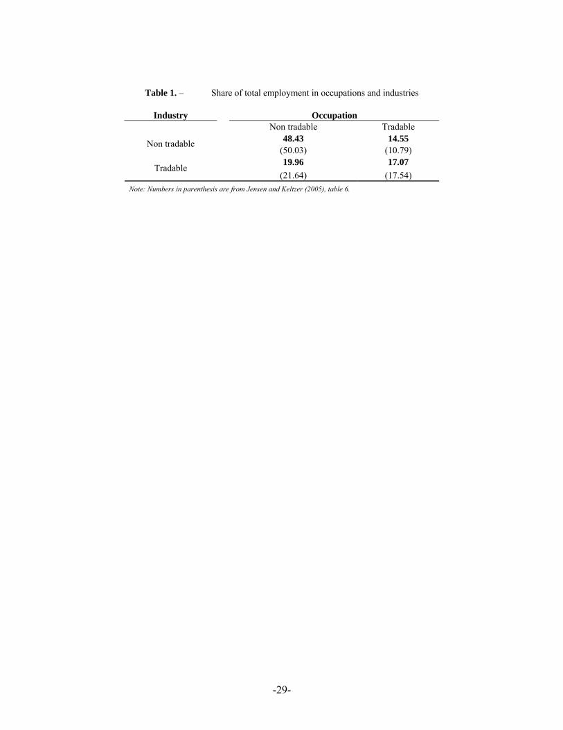
Table 1. – Share of total employment in occupations and industries

Industry Occupation Non tradable Tradable

48.43 14.55 Non tradable (50.03) (10.79) 19.96 17.07 Tradable (21.64) (17.54)

Note: Numbers in parenthesis are from Jensen and Keltzer (2005), table 6.

-29-

Table 2. – Likelihood of expressing economic insecurity: ordered probit analysis

Dependent Variable Costly job loss Insecure Regressor (1) (2) (3) (4) (5) (6) pInd .2685*** .4800*** .4802*** .1568*** .1594*** .1900*** (.0589) (.1110) (.1069) (.0283) (.0278) (.0348) pOC .1847*** .3450*** .3154*** .1702*** .1682*** .1744*** (.0575) (.1078) (.1045) (.0272) (.0267) (.0335) gHap -.5542*** -1.005*** -.1780*** -.6064*** (.0956) (.2220) (.0220) (.0931) fSit -.9898*** -.7707*** -.1239*** -.0892*** (.2658) (.2464) (.0178) (.0247) Income -.0438*** -.0560*** -.0432*** -.0239*** -.0157*** -.0104*** (.0067) (.0126) (.0129) (.0032) (.0033) (.0041) Degree -.1225*** -.2285*** -.2149*** -.0886*** -.0784*** -.0874*** (.0281) (.0575) (.0550) (.0118) (.0116) (.0148) Unemployment .1242*** .2017*** .1982*** .0828*** .0761*** .0906*** (.0326) (.0600) (.1982) (.0164) (.0161) (.0197) Union .4041*** .6857*** .6453*** .3716*** .3540*** .3846*** (.0692) (.1348) (.1312) (.0363) (.0355) (.0492) Self -.3648*** -.6402*** -.5633*** -.3331*** -.3290*** -.3468*** (.1010) (.1807) (.1731) (.0397) (.0387) (.0510) 18 to 24 -.2337** -.3233* -.3236* -.1586*** -.1380*** -.1560*** (.1004) (.1821) (.1737) (.0454) (.0449) (.0533) 40 to 54 .0507 .0145 -.0031 .1329*** .1020*** .1084*** (.0627) (.1135) (.1078) (.0297) (.0295) (.0353) Over 55 -.0711 -.1773 -.1360 .2590*** .2387*** .3026*** (.0857) (.1535) (.1475) (.0401) (.0395) (.0506) Black .3535*** .5611*** .4739*** .2113*** .1849*** .1726*** (.0751) (.1460) (.1430) (.0416) (.0411) (.0498) Other -.0332 -.0970 -.1285 .0599 .0453 .0222 (.1492) (.2756) (.2607) (.0657) (.0651) (.0761) Male .0524 .1472 .1213 .02401 .0250 .0221 (.0556) (.1030) (.0976) (.0258) (.0254) (.0298) Intercept 1 2.937*** 1.899*** 1.036 -.1959* -.9356*** -1.846*** (.2869) (.5527) (.6602) (.1144) (.1295) (.2561) Intercept 2 .5748*** -.1716 -.9723*** (.1151) (.1290) (.2287) Intercept 3 1.604*** .8485*** .1961 (.1206) (.1304) (.2150) Intercept 4 2.367*** 1.610*** 1.070*** (.1286) (.1338) (.2234) Intercept 5 2.945*** 2.180*** 1.728*** (.1377) (.1389) (.2393) Year dummies yes yes yes yes yes yes Regional dummies yes yes yes yes yes yes Instruments no no yes no no yes N 8080 8006 7959 7899 7825 7782 Log likelihood -1551 -1500 -7884 -11803 -11629 -17782 Note: Each cell reports the maximum- likelihood parameter estimate and, in parentheses, its standard error. Each model includes the following base case: female, white, non-union, who lived in the northeast in 1998 and worked in an occupation and industry safe from offshoring. The heteroskedastic robust standard errors are adjusted for respondents’ past financial situations. gHap likely being endogenous, survey questions on marital status, occupational happiness, financial satisfaction, and friendship happiness are used as instruments. * Significant at the 90 percent level. ** Significant at the 95 percent level. ***Significant at the 99 percent level.

-30-

Table 3. – Marginal effects on base-case probability

Dependent Variable Costly Job Loss Insecure

no=0 yes=1 0 1 2 3 4 5 Base-case probability .9377 .0623 .2212 .2366 .3220 .1423 .0493 .0286 pInd -.0135 .0135 -.0330 -.0239 .0149 .0216 .0113 .0090 pOC -.0089 .0089 -.0303 -.0220 .0138 .0198 .0104 .0083 gHap .0283 -.0283 .1053 .0764 -.0476 -.0689 -.0362 .0289 fSit .0217 -.0217 .0155 .0112 -.0070 -.0101 -.0053 -.0042 Income .0012 -.0012 .0018 .0013 -.0008 -.0012 -.0006 -.0005 Degree .0060 -.0060 .0152 .0110 -.0069 -.0099 -.0052 -.0042 Unemployment -.0056 .0056 -.0157 -.0114 .0071 .0103 .0054 .0043 Union -.0182 .0182 -.0668 -.0484 .0302 .0437 .0230 .0183 self .0159 -.0159 .0602 .0437 -.0272 -.0394 -.0207 -.0165 18 to 24 .0091 -.0091 .0271 .0197 -.0123 -.0177 -.0093 -.0074 40 to 54 .0000 -.0000 -.0188 -.0137 .0085 .0123 .0065 .0052 Over 55 .0038 -.0038 -.0525 .0381 .0238 .0344 .0181 .0144 Black -.0134 .0134 -.0300 -.0217 .0136 .0196 .0103 .0082 Other .0036 -.0036 -.0039 -.0028 .0017 .0025 .0013 .0011 Male -.0034 .0034 -.0038 -.0028 .0017 .0025 .0013 .0011 d_1978 -.0024 .0024 .0019 .0014 -.0009 -.0012 -.0007 -.0005 d_1983 -.0088 .0088 -.0142 -.0103 .0064 .0093 .0049 .0039 d_1985 -.0096 .0096 -.0070 -.0050 .0031 .0046 .0024 .0019 d_1988 -Base Year- d_1989 .0008 -.0008 .0063 .0045 -.0028 -.0041 -.0022 -.0017 d_1990 -.0004 .0004 -.0123 -.0089 .0056 .0081 .0042 .0034 d_1991 -.0196 .0196 -.0313 -.02274 .0142 .0205 .0108 .0086 d_1993 -.0227 .0227 -.0447 -.0324 .0202 .0293 .0154 .0123 d_1994 -.0163 .0163 -.0543 -.0394 .0246 .0355 .0187 .0149 d_1996 -.0174 .0174 -.0283 -.0205 .0128 .0185 .0097 .0078 d_1998 -.0149 .0149 -.0251 -.0182 .0113 .0164 .0086 .0069 d_2000 -.0067 .0067 -.0034 -.0024 .0015 .0022 .0012 .0009 d_2002 -.0147 .0147 -.0329 -.0239 .0149 .0215 .0113 .0090 d_2004 -.0257 .0257 -.0519 -.0376 .0235 .0340 .0178 .0142 Note: The average marginal effects presented in this table correspond to ordered probit models (3) and (6) in Table 2. An insecure value of 5 suggests the workers economic insecurity is high and a value of 0 suggests the worker is very secure.

-31-

Table 4. – Regional cohort, pseudo-panel model

N=153 Dependent variable costly job loss insecure Regressor (1) (2) (3) (4) (5) (6) pInd .0548 .0607 .0773*** .5478** .5535** .6715*** (.0475) (.0424) (.0298) (.2724) (.2710) (.2553) pOC -.0441 -.0103 -.0518** -.0902 .0148 -.0293 (0445) (.0400) (.0235) (.2554) (.0599) (.2556) Degree -.0189 -.0056 -.0240* -.3387*** -.2960*** -.3519*** (.0164) (.0147) (.0125) (.0940) (.0940) (.0829) Unemployment .0128*** .0147*** .0132*** .1079*** .1016*** .1128*** (.0030) (.0023) (.0026) (.0172) (.0156) (.0167) Income .0023 .0008 .0041** .0045 .0164 .0108 (.0031) (.0022) (.0020) (.0175) (.0156) (.0164) d_1977 -.0010 -.2965 .1627 -.0968 -.0239 -.4853 (.0206) (.6509) (.5591) (.1184) (.7048) (.7145) d_1978 .0014 -.1776 .4413 -.1649 -.5205 -1.062 (.0194) (.6321) (.9233) (.1114) (.6771) (.7264) d_1982 .0035 -.2657 .1958 -.0805 .0098 -.5158 (.0201) (.6318) (.5743) (.1155) (.6785) (.6471) d_1983 .0146 .0242 .5603 -.0158 .3059 -.0323 (.0188) (.5913) (.5589) (.1079) (.6383) (.5903) d_1985 -.0015 -.0489 -.0215 -.0078 .2416 -.0073 (.0149) (.5147) (.5021) (.0857) (.5360) (.5129) d_1986 .0176 .2655 .5456 -.0566 -.3000 -.4627 (.0146) (.5011) (.4917) (.0837) (.5202) (.5091) d_1988 -Base Year- d_1989 -.0040 -.1909 -.7594 .0312 .0471 .1737 (.0140) (.4933) (.5532) (.0806) (.5073) (.4858) d_1990 -.0074 -.4379 -.3282 .0369 .1135 .1510 (.0143) (.5018) (.4862) (.0818) (.5158) (.4916) d_1991 .0085 .4707 .2221 .1078 .7504 .5795 (.0146) (.5099) (.4954) (.0835) (.5263) (.5016) d_1993 0.0221 .8816* .7270 .2032** 1.387*** 1.107** (.0148) (.5164) (.5013) (.0850) (.5360) (.5087) d_1994 .0105 .4339 .2884 .2627*** 1.679*** 2.048*** (.0148) (.5156) (.4964) (.0849) (.5324) (.5176) d_1996 0.0053 .2944 .0342 .2212** 1.258** 1.653*** (.0157) (.5304) (.5307) (.0902) (.5558) (.5696) d_1998 .0080 .6369 .0347 .1555 .5717 1.336 (.0193) (.6092) (.5960) (.1110) (.6585) (.9533) d_2000 -.0113 -.1433 -2.200** .0249 -.3714 -.1060 (.0234) (.6991) (1.127) (.1342) (.7767) (.8085) d_2002 .0096 .5895 .0034 .1653 .5713 .6774 (.0244) (.7555) (.5909) (.1403) (.8325) (.7312) d_2004 .0080 .4299 -.0435 .2610* 1.137 1.325 (.0261) (.8034) (.6016) (.1501) (.8869) (.8708) Intercept -.0042 -.1353 -.0575 -.0602 -.3697 -.2793 (.0107) (.3739) (.3582) (.0615) (.3870) (.3661) Heteroskedascity correction Region Year Region Year R² .42 .57 .65 .59 .61 .63 Note: Each cell reports the coefficient and, in parentheses, its standard error. Heteroskedastic standard errors are calculated using the standard deviation of the ordinary-least-squares residuals. Coefficients on demographic controls are not reported. See appendix table 3 for analysis of residuals. ** Significant at the 95 percent level. ***Significant at the 99 percent level.

-32-

Table 5. – Demand for social insurance by level of economic insecurity

Mean Upper Bound

Lower Bound

Standard Error Observations

By costly job loss 1 = Yes 0.478 0.518 0.438 0.020 446 0 = No 0.415 0.425 0.405 0.005 7336 By insecure 5 0.508 0.573 0.443 0.033 185 4 0.471 0.516 0.426 0.023 356 3 0.419 0.446 0.392 0.014 1091 2 0.417 0.435 0.399 0.009 2593 1 0.417 0.437 0.397 0.01 1918 0 0.402 0.424 0.380 0.011 1639 Entire sample 0.419 0.429 0.409 0.005 7782 Note: Upper and lower bounds represent 95 percent confidence intervals.

-33-

Appendix A.1. Summary Statistics

Years: pre and post New Economy Variable 1978-1991 1992-2004

Mean Standard deviation Mean

Standard deviation Net ∆

Costly Job Loss* 0.060 0.237 0.054 0.226 - Insecure 1.634 1.237 1.637 1.203 + liklose* 0.049 0.216 0.042 0.201 - HardFind* 0.412 0.492 0.396 0.489 - pIND* 0.327 0.469 0.303 0.460 - pOC* 0.375 0.484 0.364 0.481 - gHap 2.237 0.594 2.215 0.585 - fSit 2.312 0.761 2.321 0.754 + JobHap 3.347 0.770 3.324 0.776 - FinHap 2.032 0.741 2.034 0.729 + FrdHap 2.853 0.855 2.869 0.843 + Married 0.611 0.488 0.527 0.499 - DivSep* 0.163 0.369 0.199 0.399 + Never Married* 0.195 0.396 0.245 0.430 + Widowed* 0.032 0.175 0.029 0.168 - 18 to 24* 0.107 0.309 0.086 0.280 - 25 to 39* 0.472 0.500 0.416 0.493 - 40 to 54* 0.283 0.451 0.368 0.482 + over 55* 0.138 0.345 0.130 0.336 - Male* 0.541 0.498 0.489 0.500 - Degree 1.455 1.146 1.687 1.159 + White* 0.881 0.324 0.814 0.389 - Black* 0.098 0.297 0.125 0.330 + Other* 0.021 0.143 0.061 0.240 + Union* 0.166 0.372 0.153 0.360 - Income 0.282 4.114 -0.023 4.599 - Self* 0.132 0.339 0.131 0.338 - Unemployment* 0.070 0.018 0.054 0.013 - Observations 4314 3468 Notes: Sample is of full-time workers; Degree 1 equals High School; Degree 2 equals Associate/Junior College; due to data manipulation we cannot convert Income into a dollar value.

* Mean value represents the percentage of total sample, for example 54 percent of the 1978-1991 sample is male.

-34-

A.2. Percent of total employment by region: BLS

New England

Mid Atlantic EaNoCen WeNoCen SouAtl ESouCen WeSoCen Mountian Pacific

1977 0.0584 0.1617 0.1918 0.0823 0.1595 0.0614 0.0996 0.0475 0.1377 1978 0.0582 0.1601 0.1903 0.0815 0.1605 0.0606 0.0999 0.0483 0.1406 1979 0.0582 0.1593 0.1878 0.0807 0.1605 0.0601 0.1011 0.0496 0.1426 1980 0.0583 0.1582 0.1821 0.0801 0.1619 0.0600 0.1038 0.0508 0.1449 1981 0.0584 0.1569 0.1797 0.0794 0.1632 0.0589 0.1066 0.0519 0.1450 1982 0.0588 0.1554 0.1758 0.0789 0.1649 0.0584 0.1092 0.0529 0.1456 1983 0.0590 0.1544 0.1737 0.0784 0.1664 0.0584 0.1096 0.0539 0.1462 1984 0.0592 0.1533 0.1731 0.0775 0.1682 0.0583 0.1093 0.0544 0.1466 1985 0.0591 0.1534 0.1721 0.0770 0.1697 0.0582 0.1088 0.0540 0.1477 1986 0.0589 0.1535 0.1718 0.0768 0.1720 0.0580 0.1057 0.0537 0.1496 1987 0.0587 0.1530 0.1714 0.0762 0.1739 0.0576 0.1044 0.0531 0.1517 1988 0.0582 0.1518 0.1717 0.0760 0.1751 0.0572 0.1035 0.0532 0.1534 1989 0.0573 0.1504 0.1723 0.0755 0.1756 0.0571 0.1032 0.0536 0.1550 1990 0.0565 0.1490 0.1689 0.0739 0.1773 0.0570 0.1034 0.0548 0.1591 1991 0.0555 0.1468 0.1683 0.0751 0.1785 0.0574 0.1051 0.0562 0.1571 1992 0.0549 0.1441 0.1690 0.0756 0.1792 0.0578 0.1059 0.0572 0.1562 1993 0.0544 0.1426 0.1700 0.0758 0.1798 0.0584 0.1062 0.0589 0.1540 1994 0.0535 0.1404 0.1707 0.0762 0.1802 0.0590 0.1064 0.0611 0.1525 1995 0.0530 0.1390 0.1707 0.0764 0.1806 0.0592 0.1068 0.0626 0.1517 1996 0.0529 0.1390 0.1696 0.0763 0.1810 0.0591 0.1071 0.0630 0.1520 1997 0.0528 0.1391 0.1684 0.0755 0.1815 0.0587 0.1069 0.0635 0.1535 1998 0.0526 0.1380 0.1671 0.0751 0.1821 0.0585 0.1072 0.0645 0.1550 1999 0.0525 0.1373 0.1665 0.0746 0.1829 0.0582 0.1072 0.0650 0.1558 2000 0.0522 0.1366 0.1654 0.0742 0.1841 0.0579 0.1069 0.0655 0.1572 2001 0.0522 0.1366 0.1639 0.0744 0.1839 0.0572 0.1074 0.0662 0.1582 2002 0.0523 0.1371 0.1614 0.0746 0.1846 0.0570 0.1080 0.0668 0.1583 2003 0.0519 0.1360 0.1602 0.0744 0.1861 0.0570 0.1086 0.0676 0.1581 2004 0.0513 0.1357 0.1589 0.0739 0.1872 0.0566 0.1092 0.0687 0.1584 2005 0.0508 0.1352 0.1576 0.0733 0.1890 0.0560 0.1095 0.0695 0.1590 2006 0.0504 0.1343 0.1573 0.0728 0.1913 0.0558 0.1089 0.0710 0.1583 1977-2004 0.0557 0.1471 0.1719 0.0767 0.1750 0.0583 0.1060 0.0578 0.1516 Bold Years 0.0560 0.1475 0.1716 0.0765 0.1751 0.0582 0.1061 0.0573 0.1518 GSS 0.0521 0.1460 0.1829 0.0840 0.1813 0.0645 0.0946 0.0615 0.1380 Source: GSS and the BLS.

-35-

A.3. Analysis of residuals: Predicted actual values (left) and QQ plot (right)

Costly job loss (1)

Costly job loss (2)

Costly job loss (3)

-36-

Insecure (4)

Insecure (5)

Insecure (6)

-37-

A.4. Demand for social insurance variable Primary survey question: We are faced with many problems in this country, none of which can be solved easily or inexpensively. I'm going to name some of these problems, and for each one I'd like you to tell me whether you think we're spending too much money on it, too little money, or about the right amount. Specific Areas: 1-(a) Health (b) Improving the nation’s health 2-Social Security 3-Welfare 4-(a)Education (b) Improving the nation’s education system Potential Answers: 1-Too much 2-About right 3-Not enough 4-Don’t know/ N.A. Calculation: The respondents’ answers to each question are scored as follows: too much, -1; about

right, 0; not enough, 1. The answers to the four questions are averaged to a score ranging

from -1 to 1.

A.5. Regional levels of economic insecurity and demand for social insurance

Note: The maps show the average values of insecure (left) and demand for increased funding for government programs (right) by census region over the period from 1977 to 2004. Source: GSS and authors’ calculations.

-38-

A. 6. Construction of Variables

Variable Range of Values Calculation costly job loss (CjL) 0 to 1 if θ = "very likely" or "somewhat likely and if π= "not easy at all" then

CjL=1 else CjL=0. like lose (LiL) 0 to 1 if θ = "very likely" then LiL=1 else LiL=0. hard find (HdF) 0 to 1 if π= "not easy at all" then HdF=1 else HdF=0. insecure (InS) 0 to 5 If θ = "very likely" then InSa=3; if θ = "somewhat likely" then InSa=2, if θ =

"not too likely" then InSa=1; if θ = 'not at all likely' then InSa = 0. If π = "not easy at all" then InSb = 2; if π = "somewhat easy" then InSb = 1; if π = "very easy" then InSb = 0. InS = InSa + InSb.

pInd 0 to 1 pInd = 1 if Gini class = 0 and zero otherwise. pOC 0 to 1 pOC = 1 if Gini class = 0 and zero otherwise. fSit 1 to 3 fSit =1 if respondent describes their past financail situation as "getting

worse"; fSit = 2 if respondent describes their past financail situation as "stayed the same"; fSit = 3 if respondent describes their past financail situation as "getting better".

gHap 1 to 3 gHap =1 if respondent describes themselves as "not too happy"; gHap = 2 if respondent describes themselves as "happy"; gHap = 3 if respondent describes themselves as "very happy".

Income* 1 to 9 Income =1 if respondents household income is in the lowest bracket; Income = 9 if respondents household income is in highest bracket. Regional models: real household income, as reported by the BEA.

Degree 1 to 5 if Degree = "less than high school" then Degree = 1; if Degree = "High School" then Degree = 2; if Degree = "Associate/Junior College" then Degree = 3; if Degree = "Bachelor" then Degree = 4; if Degree = "Advanced Degree" then Degree = 5.

Unemployment 2.8 to 12.5 regional unemployment rate, as reported by the BLS Union 0 to 1 Union = 1 if respondent answered "Yes" or "Yes, Both"; Union = 0 if

respondent answered "No" or "Spouse." Self 0 to 1 Self = 1 if employment status = "self employed" and zero otherwise 18 to 24 0 to 1 18 to 24 = 1 if 18 ≤ respondent age < 25 and zero otherwise. 25 to 39 0 to 1 25 to 39= 1 if 25 ≤ respondent age < 40 and zero otherwise. 40 to 54 0 to 1 40 to 54 = 1 if 40 ≤ respondent age < 55 and zero otherwise. Over 55 0 to 1 Over 55 = 1 if 55 ≤ respondent age and zero otherwise. Black 0 to 1 Black = 1 if race = "Black" and 0 otherwise. White 0 to 1 White = 1 if race = "White" and 0 otherwise. Other 0 to 1 Other = 1 if race = "Other" and 0 otherwise. Male 0 to 1 Male = 1 if sex = "male" ; Male = 0 if sex = "Female." Married 0 to 1 Married =1 if marital status = "married" and 0 otherwise. DivSep 0 to 1 DivSep =1 if marital status = "divorced/separated" and 0 otherwise. Widowed 0 to 1 Widowed =1 if marital status = "widowed" and 0 otherwise. NevMar 0 to 1 NevMar =1 if marital status = "never married" and 0 otherwise. fSat 1 to 3 fSat =1 if respondent describes their opinion of their finances as "not

satisfied"; fSat = 2 if respondent describes their opinion of their finances as "more or less satisfied"; fSat = 3 if respondent describes their opinion of their finances as "well satisfied".

fHap 1 to 4 fHap =4 if respondent describes the frequency of social activities as "daily" or "few times a week"; fHap = 3 if respondent describes the frequency of social activities as "few times a month" or "monthly"; fHap = 2 if respondent describes the frequency of social activities as “several times a year" or "annually"; fHap = 1 if respondent describes the frequency of social activities as "never".

oHap 1 to 4 oHap =4 if respondent describes work life as "very satisfied"; oHap = 3 if respondent describes work life as "satisfied" ; oHap = 2 if respondent describes work life as "a little dissatisfied"; oHap = 1 if respondent describes work life as "very dissatisfied".

Note: θ = job loss question, π= job find question, * see note 19 for more information

-39-

-40-